Lecture 1(Chapter 1)
Introduction• This course describes statistical methods
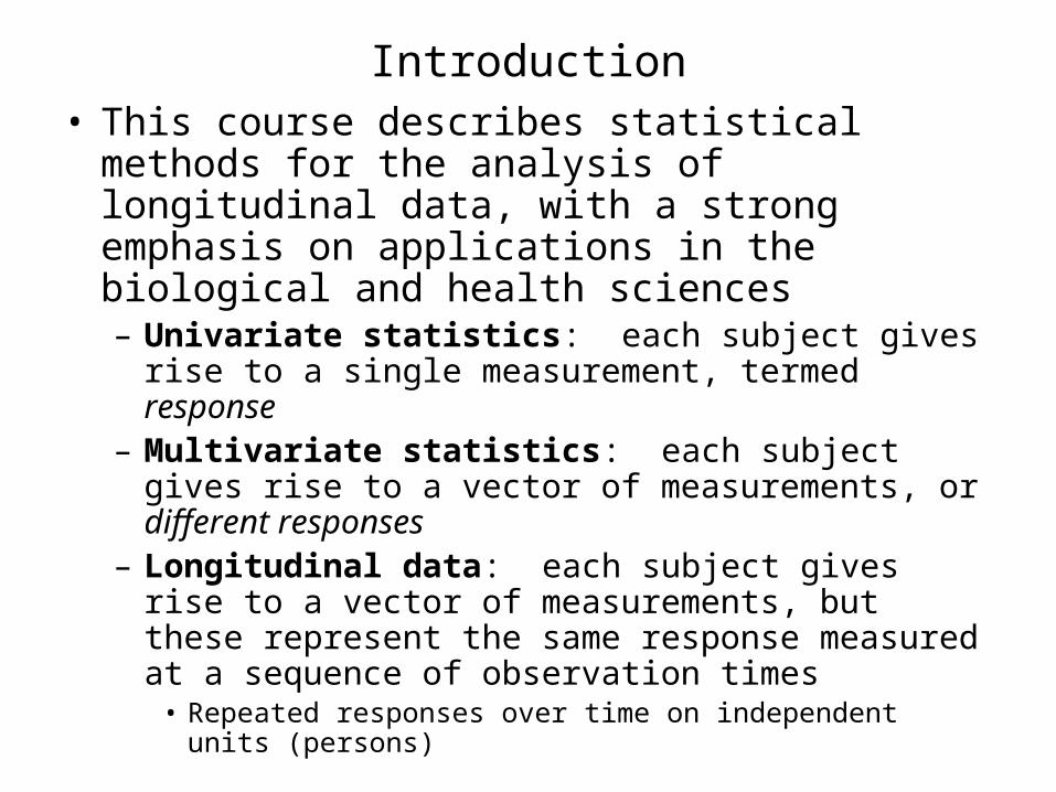
for the analysis of longitudinal data, with a strong emphasis on applications in the biological and health sciences– Univariate statistics: each subject gives rise
to a single measurement, termed response– Multivariate statistics: each subject gives
rise to a vector of measurements, or different responses
– Longitudinal data: each subject gives rise to a vector of measurements, but these represent the same response measured at a sequence of observation times
• Repeated responses over time on independent units (persons)

• Basic issues and exploratory analyses– Definition and examples of LDA– Approaches to LDA– Exploring correlation
• Statistical methods for continuous measurements– General Linear Model with correlated data
• Weighted Least Squares estimation• Maximum Likelihood estimation• Parametric models for covariance structure
• Generalized linear models for continuous/discrete responses– Marginal Models
– Log Linear Model and Poisson Model for count responses– Logistic model for binary responses– GEE estimation methods– Estimation techniques
– Random Effects Models (Multi-level models)– Transition Models
Topics

• Longitudinal study: people are measured repeatedly over time
• Cross-sectional study: a single outcome is measured for each individual
• In LDA, we can investigate:– changes over time within individuals (ageing
effects)– differences among people in their baseline
levels (cohort effects)
• LDA requires special statistical methods because the set of observations on one subject tends to be inter-correlated
Introduction

• Reading ability appears to be poorer among older children.

• Let’s assume that the reading ability of each child has been measured twice.

• LDA can distinguish between changes over time within individual & differences among people in their baseline levels

• Repeated observations
are likely to be correlated, so assumption of independence is violated
• What if we used standard regression methods anyway (ignore correlation)?– Correlation may be of scientific focus– Incorrect inference– Inefficient estimates of β
Why special methods?

• Opportunities• Distinguish “longitudinal” from “cross-
sectional” effects• Choose several targets of estimation
Challenges• Repeated observations tend to be auto-
correlated
• Correlation must be modeled
What is special about longitudinal data?

• Repeated observations on individuals• Scientific questions regression methods• Response = f(predictors)• Discrete/continuous responses and
predictors
Types of Studies• Time series studies• Panel studies (Sociology & Economics)• Prospective studies (Clinical Trials)
Characteristics

1. CD4+ cell numbers (continuous)2. Growth of Sitka spruce – tree size
(continuous)3. Protein contents of milk (continuous)4. Indonesian Children’s health study (binary)5. Analgesic Crossover trial (binary)6. Epileptic seizures (count)7. Health Effects of Air Pollution (count)
Note: All these datasets are posted on the course website
Examples

• HIV attacks CD4+ cells, which regular the body’s immunoresponse to infectious agents
• 2376 values of CD4+ cell number plotted against time since seroconversion for 369 infected men enrolled in the MACS
• Q: What is the impact of HIV infection on CD4 counts over time?
Ex: CD4+ cell numbers
Goals:1.Characterize the typical time course of
CD4+ cell depletion2.Identify factors which predict CD4+ cell
changes3.Estimate the average time course of
CD4+ cell depletion4.Characterize the degree of heterogeneity
across men in the rate of progression
Ex: CD4+ cell numbers (cont’d)

• This figure displays 2376 values of CD4+ cell numbers plotted against time since sero-conversion for 369 infected men enrolled in the MACS study.


Ex: Growth of trees
• Data for 79 trees over two growing seasons– 54 trees were grown with ozone
exposure at 70 ppb– 25 trees were grown under control
conditions• Goal: Compare the growth patterns of
trees under the two conditions

Goal: To assess the effect of ozone pollution on tree growth
Figure 1.3. Log-size of 79 sitka spruce trees over 2 growing seasons

Ex: Protein content of milk
• Milk was collected weekly for 79 Australian cows and analyzed for their protein content
• Cows were maintained on one of three diets
• Goal: To determine how diet affects the protein content in milk
• Problem: About half of the 79 sequences are incomplete (i.e. missing data)

• Barley (25 cows)
• Mixed (27 cows)
• Lupins (27 cows)

Ex: Indonesian Children’s Health Study (ICHS)
• Dr. Sommer conducted a study to determine effects of vitamin A deficiency in pre-school children
• Over 3000 children were examined for up to 6 visits to assess whether they suffered from respiratory infection or xerophthalmia (an ocular manifestation of vit A deficiency). Weight and height are also measured.
• Q: What are the predictors of infection?

Ex: ICHS (cont’d)
Goals:1. Estimate the increase in risk of
respiratory infection for children who are vitamin A deficient while controlling for other demographic factors
2. Estimate the degree of heterogeneity in the risk of disease among children

Ex: ICHS (cont’d)
Respiratory Infection (RI) i (0, 1, 0, 0, 1, 1)
Xerophthalmia i (1, 1, 0, 0, 1, 1)

Ex: Analgesic Crossover trial
• 3-period crossover trial of an analgesic drug for relieving pain for primary dysmenorrhea
• 3 levels of analgesic (control, low, and high) were given to each of the 86 women
• Women were randomized to one of the 6 possible orders for administering the 3 treatment levels
• Pain was relieved for 26% with placebo, 71% with low dose, and 80% with high dose
• Q: Treatment effect?• Q: How about carry-over effects?

Ex: Analgesic Crossover trial (cont’d)
• Ignoring the order of treatments, pain was relieved for 22 women under placebo

Ex: Epileptic seizures
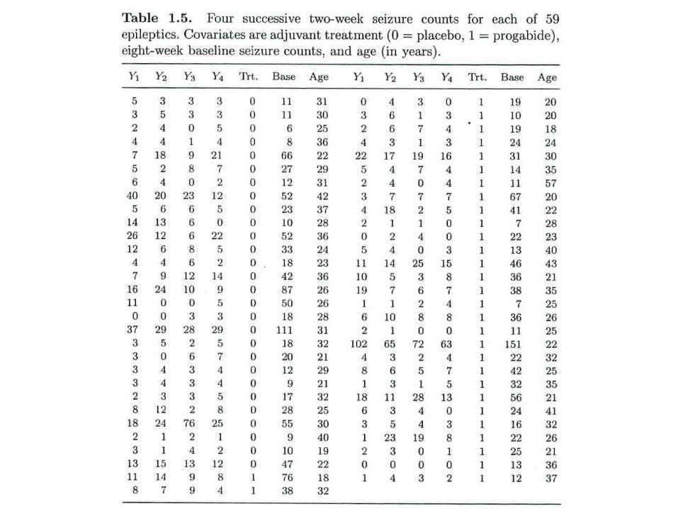
• Clinical trial of 59 epileptics• For each patient, the number of epileptic
seizures was recorded during a baseline period of 8 weeks
• Patients were randomized to treatment with the antiepileptic drug progabide or placebo
• Number of seizures was then recorded in 4 consecutive 2-week intervals
• Q: Does progabide reduce the epileptic seizure rate?

• Placebo
• Progabide
What do these examples have in common?
• These are repeated observations on each experimental unit
• Units can be assumed independent of one another
• Multiple responses within each unit are likely to be correlated
• The objectives can be formulated as regression problems whose purpose is to describe the dependence of the response on explanatory variables
• The choice of the statistical model must depend on the type of the outcome variable

Course Overview
• Scientific objectives include:– Characterize change– Component of variation– Hypothesis testing
• We will focus on regression models• We will consider (up to 6) case studies
in detail• Computing using Stata will be
introduced (SAS macros will be provided)

Notation

Notation (cont’d)
Regression Model
(n1 x 1) (n1 x p) (p x 1) (n1 x 1)
Suppose:

Cross-sectional versus Longitudinal Study
with respect to its baseline value

Cross-sectional versus Longitudinal Study (cont’d)

Cross-sectional versus Longitudinal Study (cont’d)

Cross-sectional versus Longitudinal Study (cont’d)
Example

Example

Approaches to LDA
• If we have one observation on each experimental unit, we are confined to modeling the population average of Y, called marginal mean response
• If we have repeated measurements, there are several approaches we can use:
1. Reduce the repeated values into one or two summary variables
2. Analyze each summary variable as a function of covariates xi (two-stage analysis)

Approaches to LDA (cont’d)
For example, in the Sitka spruce data, we can:
1. Estimate the growth rate of each tree2. Compare the rates across ozone
groupsxij = xi
Explanatory variables do not change over time.
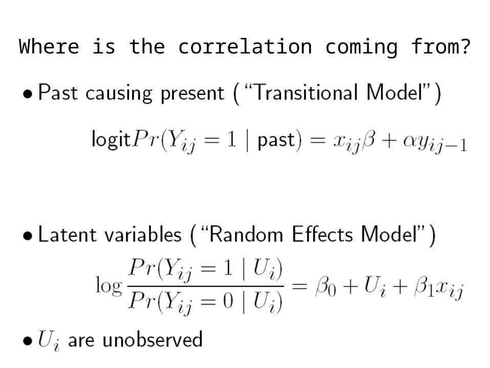
Where is the correlation coming from?

Approaches to LDA

ICHS Example
To illustrate the three approaches, we consider the ICHS example.
Let:

Compare with Standard logistic regression model (only one measurement for each subject)
Marginal Models

Random Effects Models
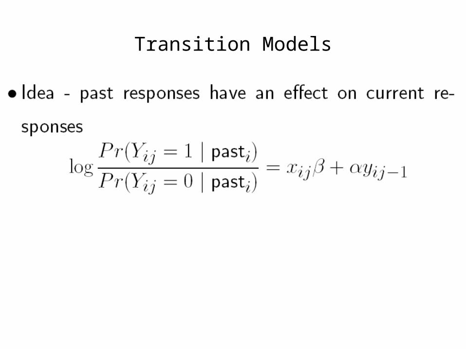
Transition Models

Appropriate EDA techniques
• Lines plots (spaghetti plots)• Average and distribution plots (boxplot,
quantiles)• Empirical covariance• Residual “pairs” plots• Variograms (for unequally spaced
observations)• Scatterplot of a response against time• Smoothing to highlight the typical
response as a function of an explanatory variable

Why LDA?
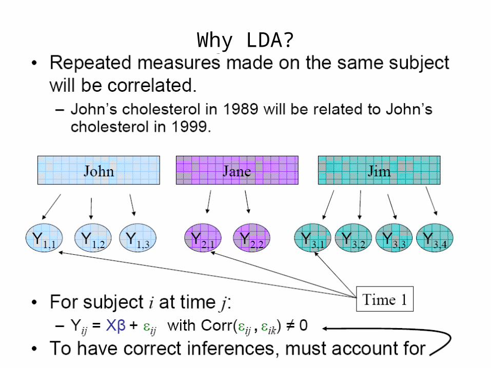
Why LDA?

Visualize the Independence Case:

Visualize the Correlation Case:
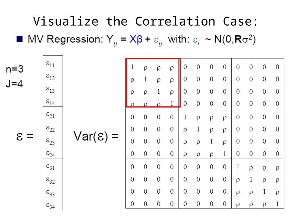
Visualize the Correlation Case:

Visualize the Correlation Case:

Compare with Independence Case:

LDA & Correlation:

LDA & Correlation:
…LDA takes care of R
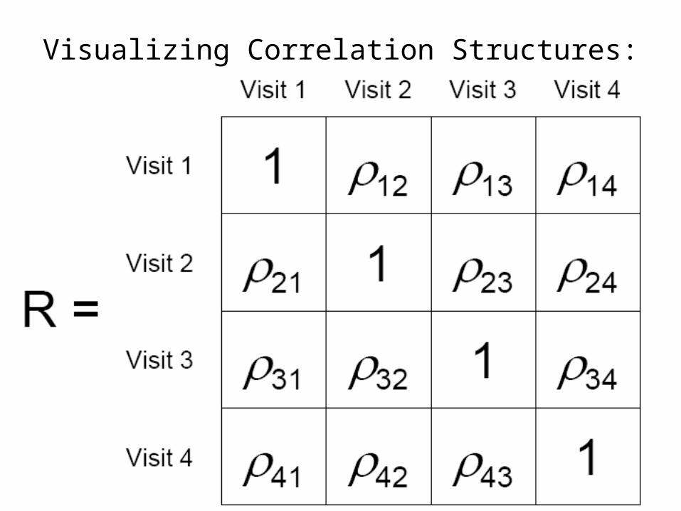
Visualizing Correlation Structures:

Visualizing Correlation Structures:

Visualizing Correlation Structures:
Uniform, Exchangeable, Compound Symmetry…

Visualizing Correlation Structures:
Uniform, Exchangeable, Compound Symmetry…

Visualizing Correlation Structures:
Uniform, Exchangeable, Compound Symmetry…
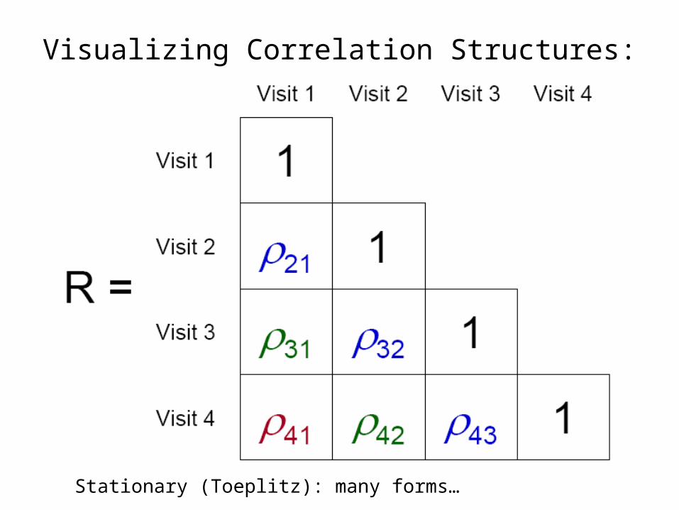
Visualizing Correlation Structures:
Stationary (Toeplitz): many forms…

Visualizing Correlation Structures:
Stationary (Toeplitz): decreasing

Visualizing Correlation Structures:
Stationary (Toeplitz): “mdependent” (ha) (m=2)
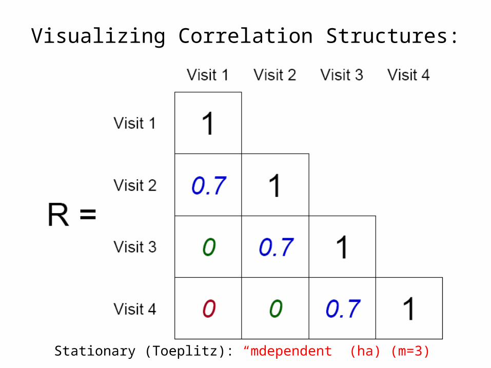
Visualizing Correlation Structures:
Stationary (Toeplitz): “mdependent” (ha) (m=3)

Visualizing Correlation Structures:
Stationary (Toeplitz): Autoregressive (AR)

Visualizing Correlation Structures:
Stationary (Toeplitz): Autoregressive (AR)

Visualizing Correlation Structures:
Stationary (Toeplitz): Autoregressive (AR)
Recommended