Contents
Probability Distributions
Estimation
Hypothesis Testing: One Sample Tests Two Sample Tests
Regression
Analysis Of Variance (ANOVA)
Statistical Process Control

Probability Distributions
Lecture 01
Data and Statistics
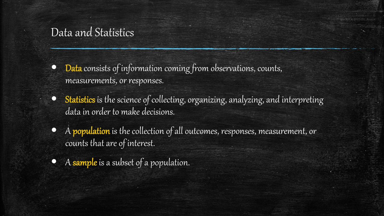
Data consists of information coming from observations, counts, measurements, or responses.
Statistics is the science of collecting, organizing, analyzing, and interpreting data in order to make decisions.
A population is the collection of all outcomes, responses, measurement, or counts that are of interest.
A sample is a subset of a population.
Populations & Samples
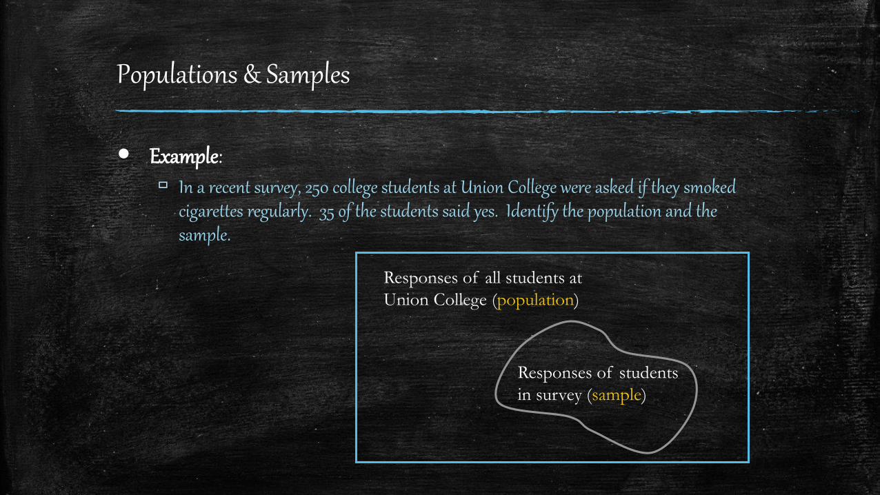
Example: In a recent survey, 250 college students at Union College were asked if they smoked
cigarettes regularly. 35 of the students said yes. Identify the population and the sample.
Responses of all students at
Union College (population)
Responses of students
in survey (sample)
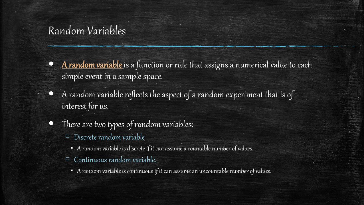
Random Variables
A random variable is a function or rule that assigns a numerical value to each simple event in a sample space.
A random variable reflects the aspect of a random experiment that is of interest for us.
There are two types of random variables: Discrete random variable▪ A random variable is discrete if it can assume a countable number of values.
Continuous random variable.▪ A random variable is continuous if it can assume an uncountable number of values.
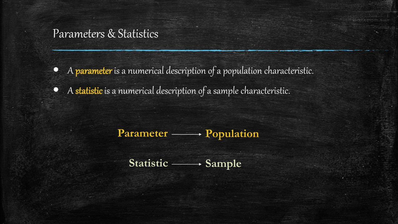
Parameters & Statistics
A parameter is a numerical description of a population characteristic.
A statistic is a numerical description of a sample characteristic.
Parameter Population
Statistic Sample
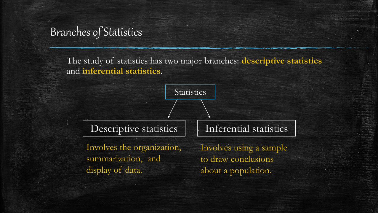
Branches of Statistics
The study of statistics has two major branches: descriptive statistics and inferential statistics.
Statistics
Descriptive statistics Inferential statistics
Involves the organization,
summarization, and
display of data.
Involves using a sample
to draw conclusions
about a population.
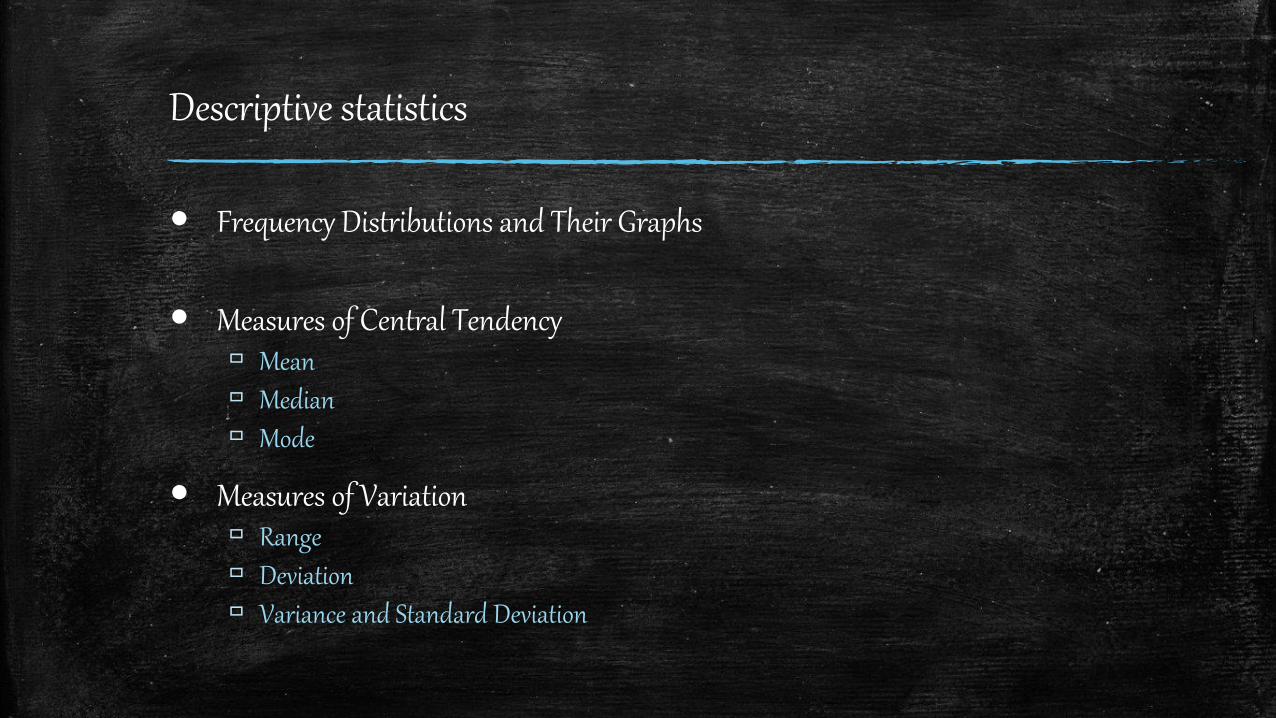
Descriptive statistics
Frequency Distributions and Their Graphs
Measures of Central Tendency Mean Median Mode
Measures of Variation Range Deviation Variance and Standard Deviation
Descriptive statistics
Measures of Position Quartiles
Interquartile Range
Box and Whisker Plot
Standard Scores
probability
Probability is how frequently we expect different outcomes to occur if we repeat the experiment over and over
Probability functions A probability function maps the possible values of random variable, say x, against
their respective probabilities of occurrence, p(x)
p(x) is a number from 0 to 1.0.
The area under a probability function is always 1.
Probability Distribution
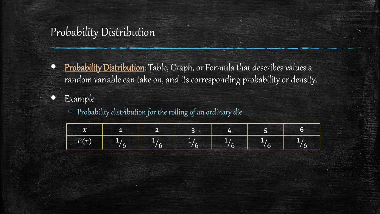
Probability Distribution: Table, Graph, or Formula that describes values a random variable can take on, and its corresponding probability or density.
Example Probability distribution for the rolling of an ordinary die
𝒙 1 2 3 4 5 6
𝑃(𝑥) 1 6 1 6 1 6 1 6 1 6 1 6
Probability Distribution
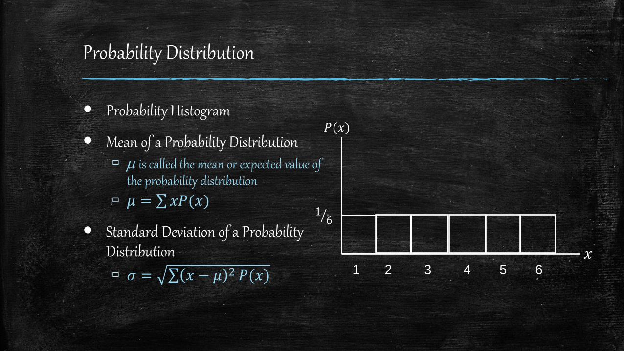
Probability Histogram
Mean of a Probability Distribution is called the mean or expected value of
the probability distribution
𝜇 = 𝑥𝑃(𝑥)
Standard Deviation of a Probability Distribution
𝜎 = 𝑥 − 𝜇 2 𝑃(𝑥)
𝑃(𝑥)
1 2 3 4 5 6
1 6
𝑥
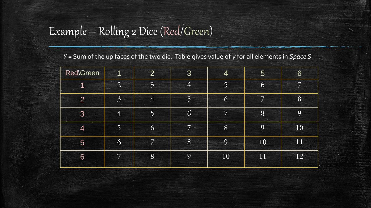
Example – Rolling 2 Dice (Red/Green)
Red\Green 1 2 3 4 5 6
1
2
3
4
5
6
Y = Sum of the up faces of the two die. Table gives value of y for all elements in Space S
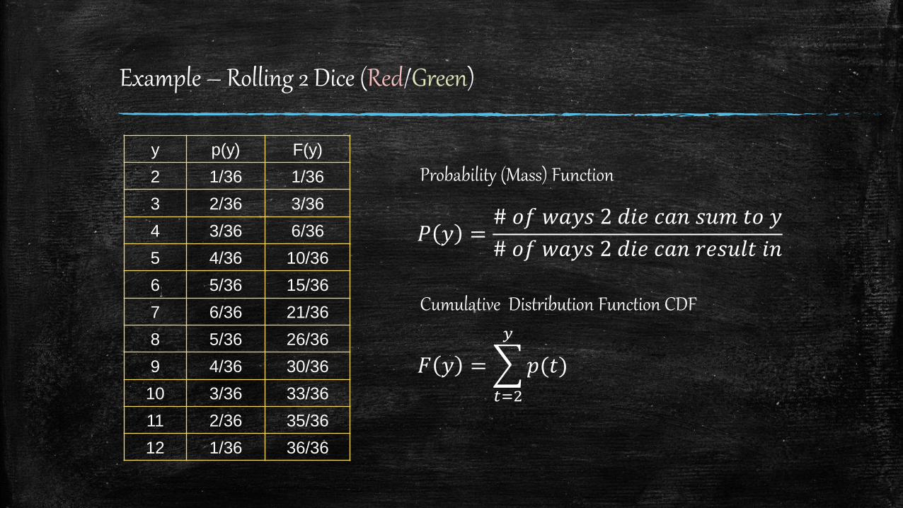
Example – Rolling 2 Dice (Red/Green)
y p(y) F(y)
2 1/36 1/36
3 2/36 3/36
4 3/36 6/36
5 4/36 10/36
6 5/36 15/36
7 6/36 21/36
8 5/36 26/36
9 4/36 30/36
10 3/36 33/36
11 2/36 35/36
12 1/36 36/36
𝑃 𝑦 =# 𝑜𝑓 𝑤𝑎𝑦𝑠 2 𝑑𝑖𝑒 𝑐𝑎𝑛 𝑠𝑢𝑚 𝑡𝑜 𝑦
# 𝑜𝑓 𝑤𝑎𝑦𝑠 2 𝑑𝑖𝑒 𝑐𝑎𝑛 𝑟𝑒𝑠𝑢𝑙𝑡 𝑖𝑛
𝐹 𝑦 =
𝑡=2
𝑦
𝑝(𝑡)
Probability (Mass) Function
Cumulative Distribution Function CDF
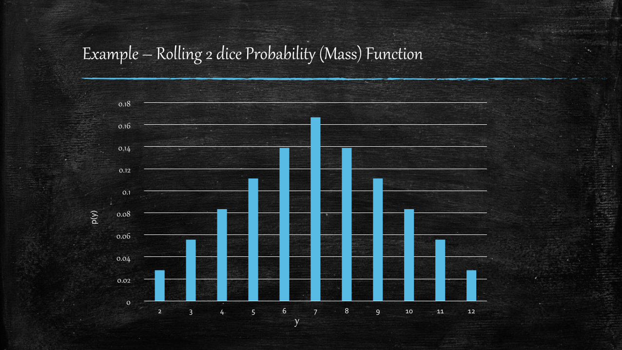
Example – Rolling 2 dice Probability (Mass) Function
0
0.02
0.04
0.06
0.08
0.1
0.12
0.14
0.16
0.18
2 3 4 5 6 7 8 9 10 11 12
p(y
)
y
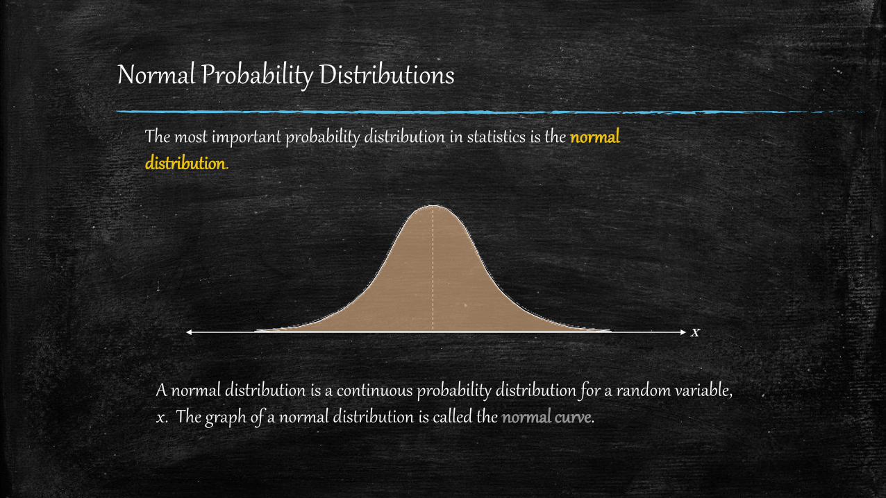
Normal Probability Distributions
The most important probability distribution in statistics is the normal distribution.
A normal distribution is a continuous probability distribution for a random variable, x. The graph of a normal distribution is called the normal curve.
x

Properties of Normal Distributions
Properties of a Normal Distribution The mean, median, and mode are equal.
The normal curve is bell-shaped and symmetric about the mean.
The total area under the curve is equal to one.
The normal curve approaches, but never touches the x-axis as it extends farther and farther away from the mean.
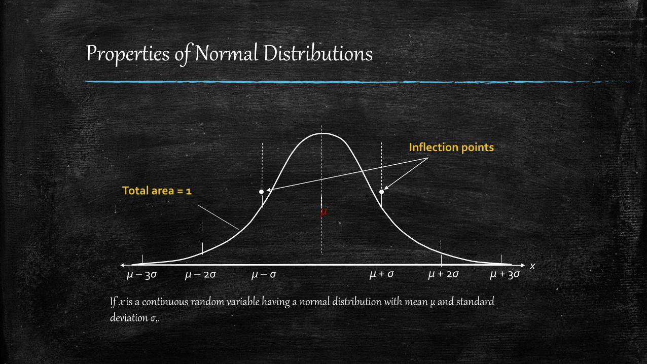
Between μ - σ and μ + σ (in the center of the curve), the graph curves downward. The graph curves upward to the left of μ - σ and to the right of μ + σ. The points at which the curve changes from curving upward to curving downward are called the inflection points.
Properties of Normal Distributions
μ 3σ μ + σμ 2σ μ σ
μ
μ + 2σ μ + 3σ
Inflection points
Total area = 1
If x is a continuous random variable having a normal distribution with mean μ and standard deviation σ,.
x
Means and Standard Deviations
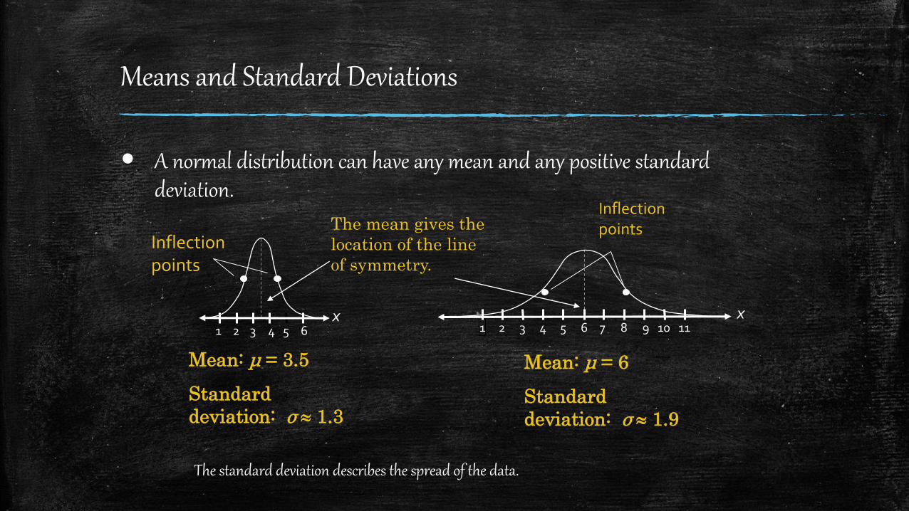
A normal distribution can have any mean and any positive standard deviation.
Mean: μ = 3.5
Standard
deviation: σ 1.3
Mean: μ = 6
Standard
deviation: σ 1.9
The mean gives the
location of the line
of symmetry.
The standard deviation describes the spread of the data.
Inflection points
Inflection points
3 61 542x
3 61 542 97 11108x
Means and Standard Deviations
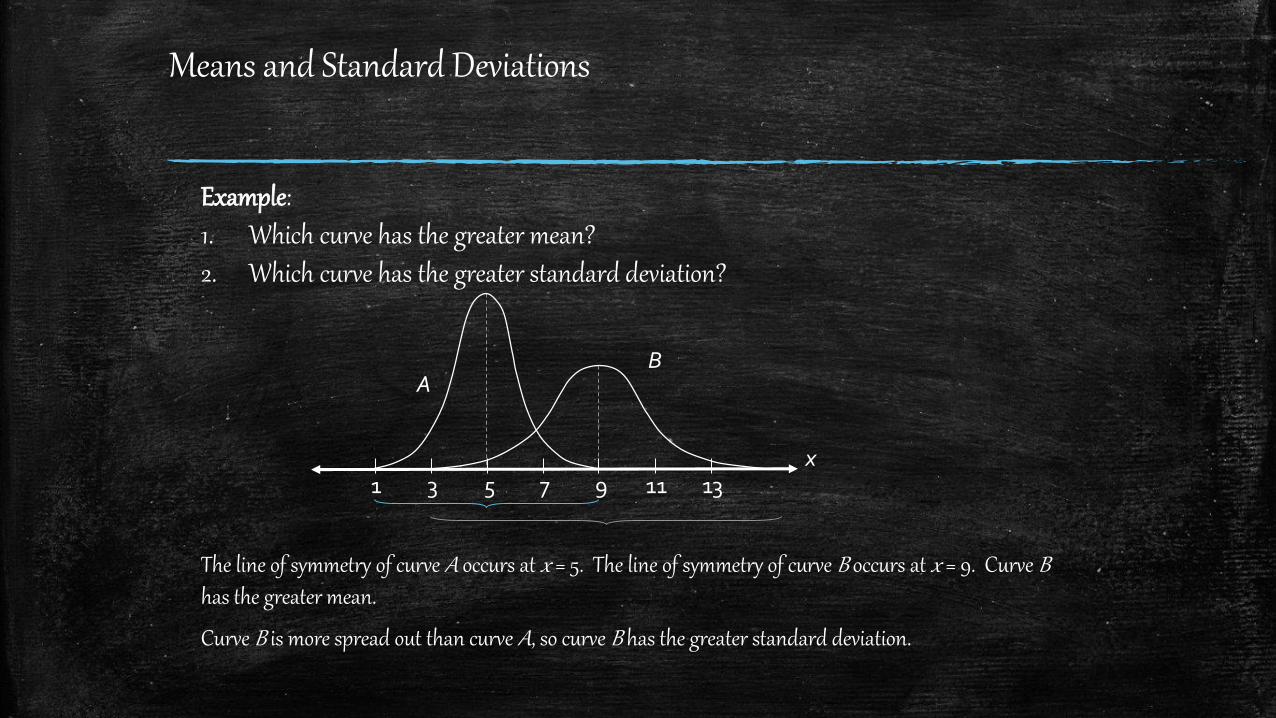
Example:1. Which curve has the greater mean?2. Which curve has the greater standard deviation?
The line of symmetry of curve A occurs at x = 5. The line of symmetry of curve B occurs at x = 9. Curve B has the greater mean.
Curve B is more spread out than curve A, so curve B has the greater standard deviation.
31 5 97 11 13
AB
x
Interpreting Graphs
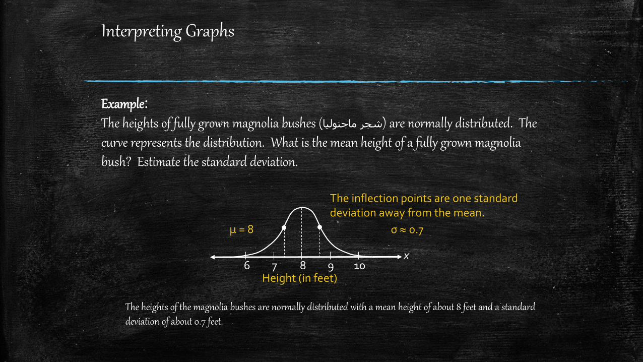
Example:The heights of fully grown magnolia bushes ( ماجنولياشجر ) are normally distributed. The curve represents the distribution. What is the mean height of a fully grown magnolia bush? Estimate the standard deviation.
The heights of the magnolia bushes are normally distributed with a mean height of about 8 feet and a standard deviation of about 0.7 feet.
μ = 8
The inflection points are one standard deviation away from the mean.
σ 0.7
6 87 9 10Height (in feet)
x
3 12 1 0 2 3
z
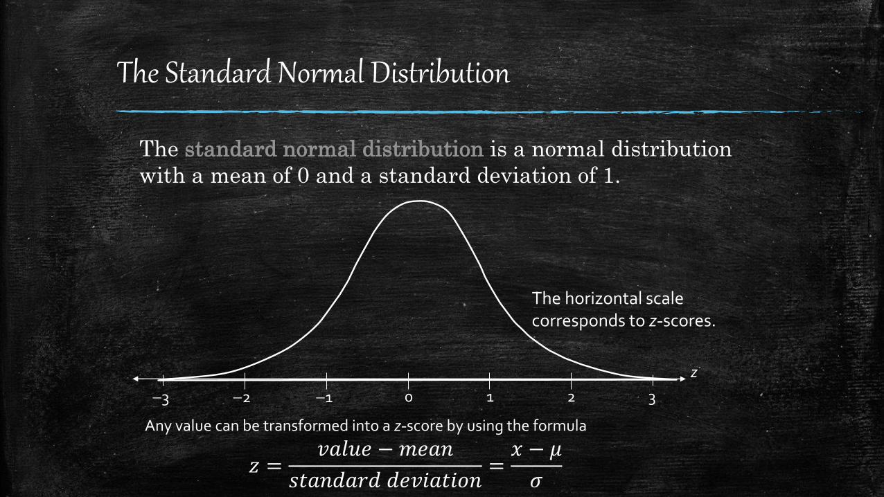
The Standard Normal Distribution
The standard normal distribution is a normal distribution
with a mean of 0 and a standard deviation of 1.
Any value can be transformed into a z-score by using the formula
The horizontal scale corresponds to z-scores.
𝑧 =𝑣𝑎𝑙𝑢𝑒 − 𝑚𝑒𝑎𝑛
𝑠𝑡𝑎𝑛𝑑𝑎𝑟𝑑 𝑑𝑒𝑣𝑖𝑎𝑡𝑖𝑜𝑛=𝑥 − 𝜇
𝜎
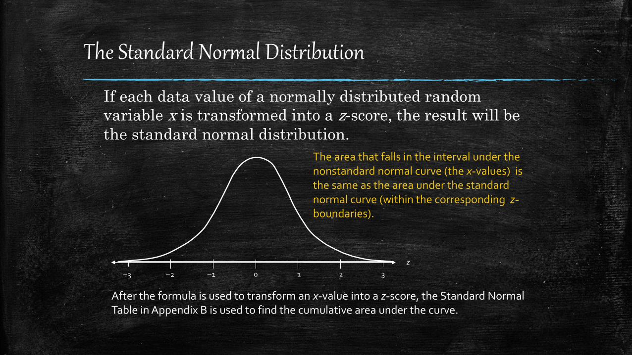
The Standard Normal Distribution
If each data value of a normally distributed random
variable x is transformed into a z-score, the result will be
the standard normal distribution.
After the formula is used to transform an x-value into a z-score, the Standard Normal Table in Appendix B is used to find the cumulative area under the curve.
The area that falls in the interval under the nonstandard normal curve (the x-values) is the same as the area under the standard normal curve (within the corresponding z-
boundaries).
3 12 1 0 2 3
z

The Standard Normal Table
Properties of the Standard Normal Distribution
1. The cumulative area is close to 0 for z-scores close to z = 3.49.
2. The cumulative area increases as the z-scores increase.
3. The cumulative area for z = 0 is 0.5000.
4. The cumulative area is close to 1 for z-scores close to z = 3.49
z = 3.49
Area is close to 0.
z = 0Area is 0.5000.
z = 3.49
Area is close to 1.z
3 12 1 0 2 3
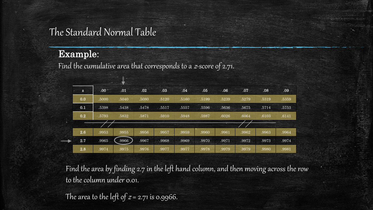
The Standard Normal Table
Example:
Find the cumulative area that corresponds to a z-score of 2.71.
z .00 .01 .02 .03 .04 .05 .06 .07 .08 .09
0.0 .5000 .5040 .5080 .5120 .5160 .5199 .5239 .5279 .5319 .5359
0.1 .5398 .5438 .5478 .5517 .5557 .5596 .5636 .5675 .5714 .5753
0.2 .5793 .5832 .5871 .5910 .5948 .5987 .6026 .6064 .6103 .6141
2.6 .9953 .9955 .9956 .9957 .9959 .9960 .9961 .9962 .9963 .9964
2.7 .9965 .9966 .9967 .9968 .9969 .9970 .9971 .9972 .9973 .9974
2.8 .9974 .9975 .9976 .9977 .9977 .9978 .9979 .9979 .9980 .9981
Find the area by finding 2.7 in the left hand column, and then moving across the row to the column under 0.01.
The area to the left of z = 2.71 is 0.9966.
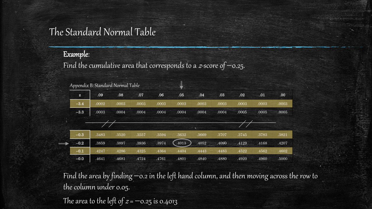
The Standard Normal Table
Example:Find the cumulative area that corresponds to a z-score of 0.25.
z .09 .08 .07 .06 .05 .04 .03 .02 .01 .00
3.4 .0002 .0003 .0003 .0003 .0003 .0003 .0003 .0003 .0003 .0003
3.3 .0003 .0004 .0004 .0004 .0004 .0004 .0004 .0005 .0005 .0005
Find the area by finding 0.2 in the left hand column, and then moving across the row to the column under 0.05.
The area to the left of z = 0.25 is 0.4013
0.3 .3483 .3520 .3557 .3594 .3632 .3669 .3707 .3745 .3783 .3821
0.2 .3859 .3897 .3936 .3974 .4013 .4052 .4090 .4129 .4168 .4207
0.1 .4247 .4286 .4325 .4364 .4404 .4443 .4483 .4522 .4562 .4602
0.0 .4641 .4681 .4724 .4761 .4801 .4840 .4880 .4920 .4960 .5000
Appendix B: Standard Normal Table
Guidelines for Finding Areas
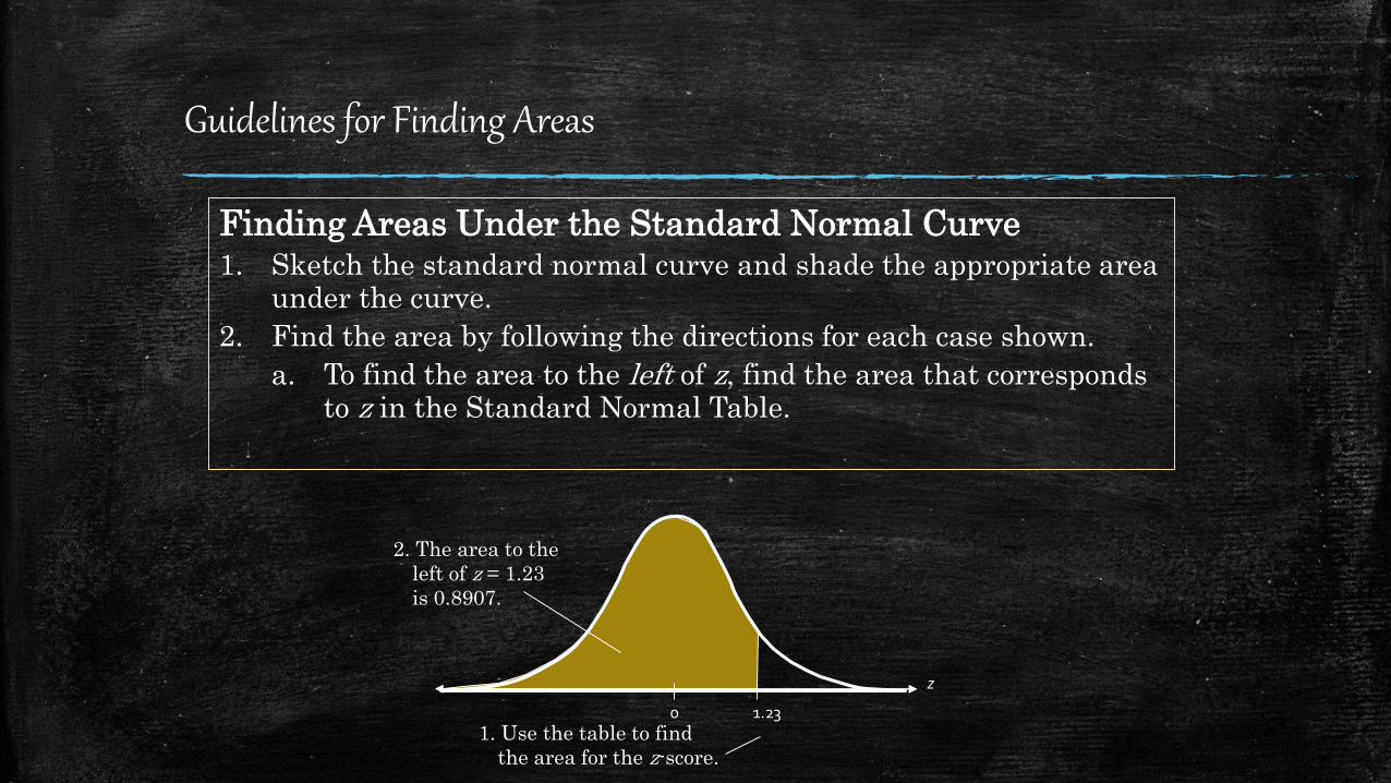
Finding Areas Under the Standard Normal Curve1. Sketch the standard normal curve and shade the appropriate area
under the curve.
2. Find the area by following the directions for each case shown.
a. To find the area to the left of z, find the area that corresponds to z in the Standard Normal Table.
1. Use the table to find
the area for the z-score.
2. The area to the
left of z = 1.23
is 0.8907.
1.230
z
Guidelines for Finding Areas
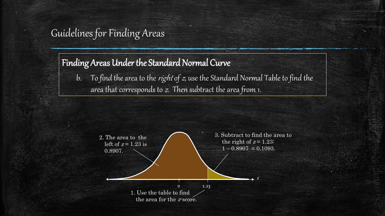
Finding Areas Under the Standard Normal Curve
b. To find the area to the right of z, use the Standard Normal Table to find the area that corresponds to z. Then subtract the area from 1.
3. Subtract to find the area to
the right of z = 1.23:
1 0.8907 = 0.1093.
1. Use the table to find
the area for the z-score.
2. The area to the
left of z = 1.23 is
0.8907.
1.230
z
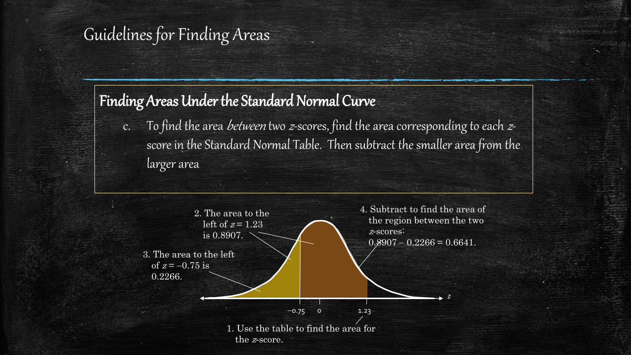
Finding Areas Under the Standard Normal Curve
c. To find the area between two z-scores, find the area corresponding to each z-score in the Standard Normal Table. Then subtract the smaller area from the larger area
Guidelines for Finding Areas
4. Subtract to find the area of
the region between the two
z-scores:
0.8907 0.2266 = 0.6641.
1. Use the table to find the area for
the z-score.
3. The area to the left
of z = 0.75 is
0.2266.
2. The area to the
left of z = 1.23
is 0.8907.
1.230
z
0.75
Guidelines for Finding Areas
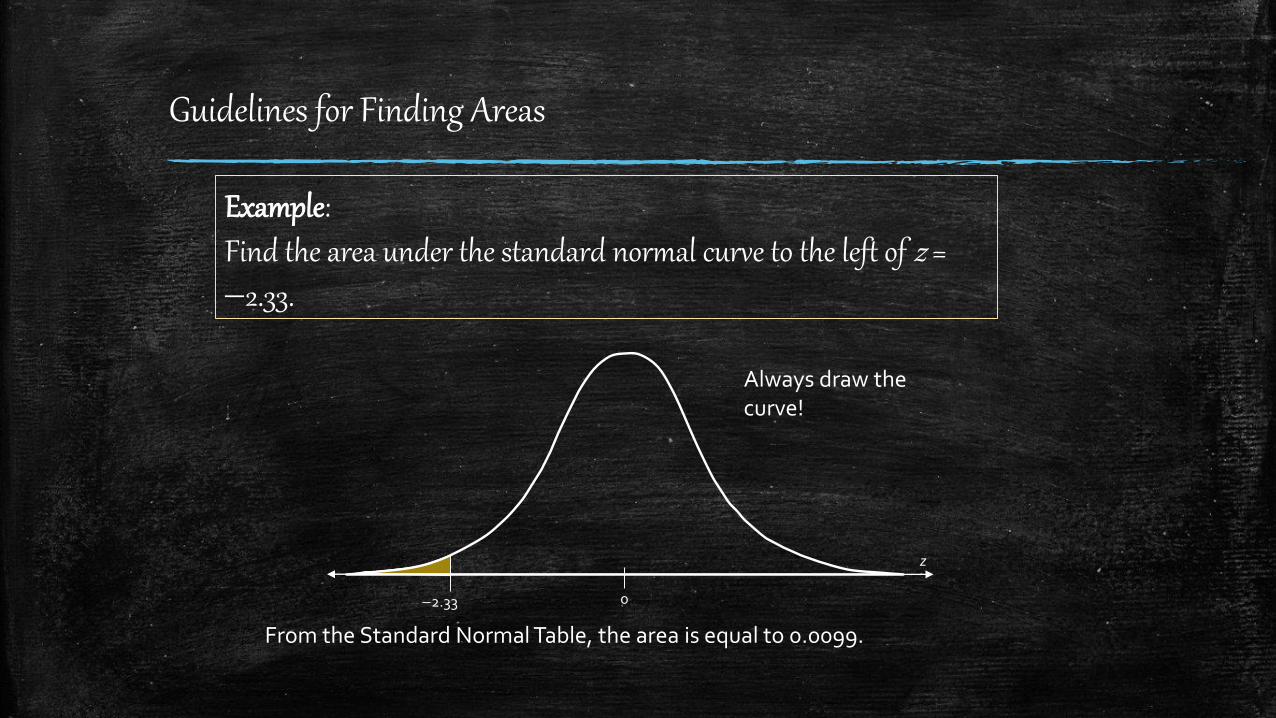
Example:Find the area under the standard normal curve to the left of z = 2.33.
From the Standard Normal Table, the area is equal to 0.0099.
Always draw the curve!
2.33 0
z
Guidelines for Finding Areas
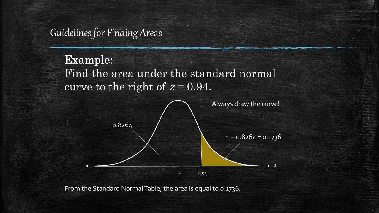
Example:
Find the area under the standard normal
curve to the right of z = 0.94.
From the Standard Normal Table, the area is equal to 0.1736.
Always draw the curve!
0.8264
1 0.8264 = 0.1736
0.940
z
Guidelines for Finding Areas
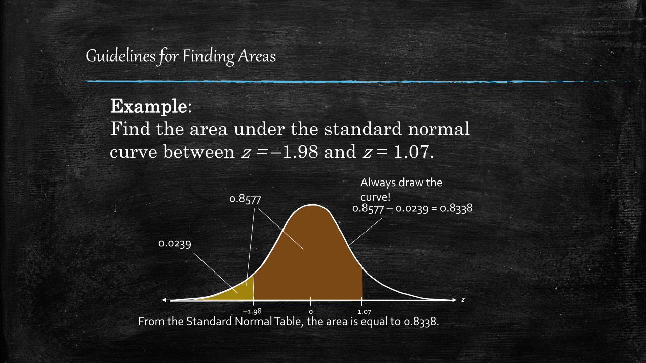
Example:
Find the area under the standard normal
curve between z = 1.98 and z = 1.07.
From the Standard Normal Table, the area is equal to 0.8338.
Always draw the curve!
0.8577 0.0239 = 0.83380.8577
0.0239
1.070
z
1.98
Probability and Normal Distributions
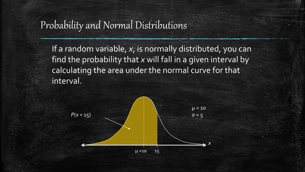
If a random variable, x, is normally distributed, you can find the probability that x will fall in a given interval by calculating the area under the normal curve for that interval.
P(x < 15)μ = 10σ = 5
15μ =10
x
Probability and Normal Distributions
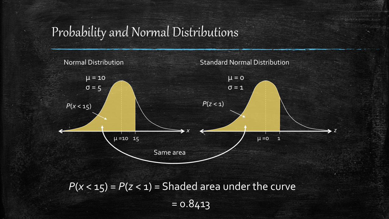
Same area
P(x < 15) = P(z < 1) = Shaded area under the curve
= 0.8413
15μ =10
P(x < 15)
μ = 10σ = 5
Normal Distribution
x1μ =0
μ = 0σ = 1
Standard Normal Distribution
z
P(z < 1)
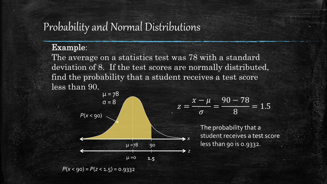
Example:
The average on a statistics test was 78 with a standard
deviation of 8. If the test scores are normally distributed,
find the probability that a student receives a test score
less than 90.
Probability and Normal Distributions
P(x < 90) = P(z < 1.5) = 0.9332
The probability that a student receives a test score less than 90 is 0.9332.
μ =0z
?1.5
90μ =78
P(x < 90)
μ = 78σ = 8
x
𝑧 =𝑥 − 𝜇
𝜎=90 − 78
8= 1.5
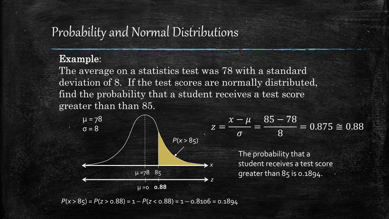
Example:
The average on a statistics test was 78 with a standard
deviation of 8. If the test scores are normally distributed,
find the probability that a student receives a test score
greater than than 85.
Probability and Normal Distributions
P(x > 85) = P(z > 0.88) = 1 P(z < 0.88) = 1 0.8106 = 0.1894
The probability that a student receives a test score greater than 85 is 0.1894.
μ =0z
?0.88
85μ =78
P(x > 85)
μ = 78σ = 8
x
𝑧 =𝑥 − 𝜇
𝜎=85 − 78
8= 0.875 ≅ 0.88
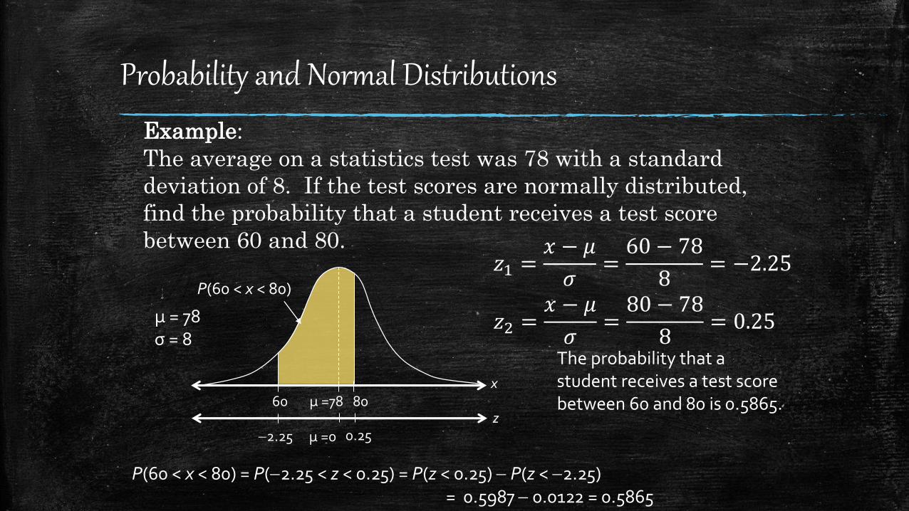
Example:
The average on a statistics test was 78 with a standard
deviation of 8. If the test scores are normally distributed,
find the probability that a student receives a test score
between 60 and 80.
Probability and Normal Distributions
P(60 < x < 80) = P(2.25 < z < 0.25) = P(z < 0.25) P(z < 2.25)
The probability that a student receives a test score between 60 and 80 is 0.5865.
μ =0z
?? 0.252.25
= 0.5987 0.0122 = 0.5865
60 80μ =78
P(60 < x < 80)
μ = 78σ = 8
x
𝑧1 =𝑥 − 𝜇
𝜎=60 − 78
8= −2.25
𝑧2 =𝑥 − 𝜇
𝜎=80 − 78
8= 0.25
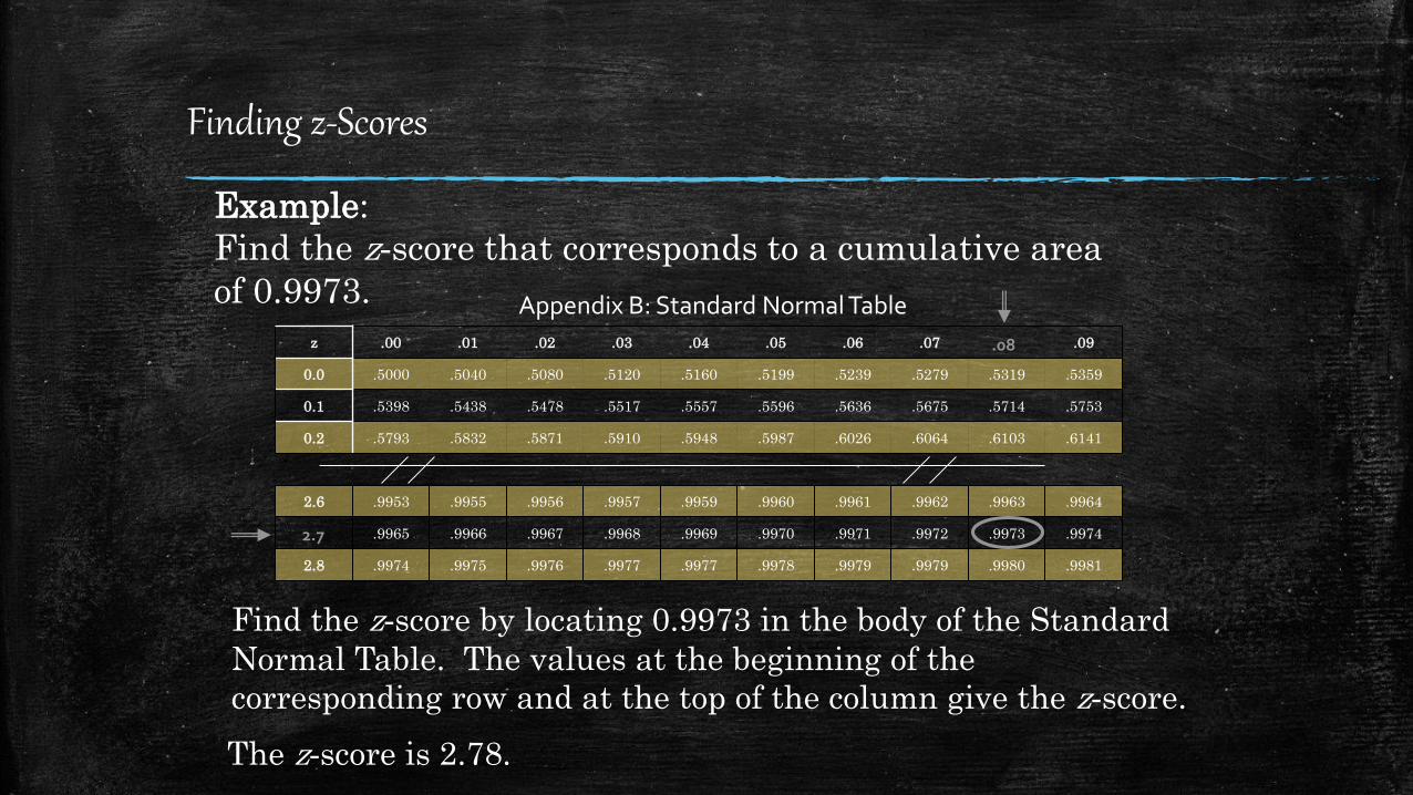
Finding z-Scores
Example:
Find the z-score that corresponds to a cumulative area
of 0.9973.
z .00 .01 .02 .03 .04 .05 .06 .07 .08 .09
0.0 .5000 .5040 .5080 .5120 .5160 .5199 .5239 .5279 .5319 .5359
0.1 .5398 .5438 .5478 .5517 .5557 .5596 .5636 .5675 .5714 .5753
0.2 .5793 .5832 .5871 .5910 .5948 .5987 .6026 .6064 .6103 .6141
2.6 .9953 .9955 .9956 .9957 .9959 .9960 .9961 .9962 .9963 .9964
2.7 .9965 .9966 .9967 .9968 .9969 .9970 .9971 .9972 .9973 .9974
2.8 .9974 .9975 .9976 .9977 .9977 .9978 .9979 .9979 .9980 .9981
Find the z-score by locating 0.9973 in the body of the Standard
Normal Table. The values at the beginning of the
corresponding row and at the top of the column give the z-score.
The z-score is 2.78.
Appendix B: Standard Normal Table
2.7
.08
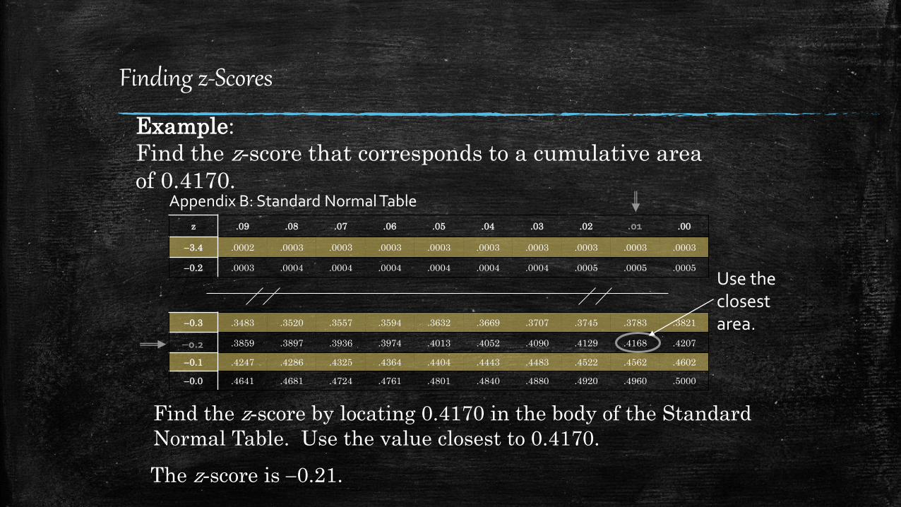
Finding z-Scores
Example:
Find the z-score that corresponds to a cumulative area
of 0.4170.
z .09 .08 .07 .06 .05 .04 .03 .02 .01 .00
3.4 .0002 .0003 .0003 .0003 .0003 .0003 .0003 .0003 .0003 .0003
0.2 .0003 .0004 .0004 .0004 .0004 .0004 .0004 .0005 .0005 .0005
Find the z-score by locating 0.4170 in the body of the Standard
Normal Table. Use the value closest to 0.4170.
0.3 .3483 .3520 .3557 .3594 .3632 .3669 .3707 .3745 .3783 .3821
0.2 .3859 .3897 .3936 .3974 .4013 .4052 .4090 .4129 .4168 .4207
0.1 .4247 .4286 .4325 .4364 .4404 .4443 .4483 .4522 .4562 .4602
0.0 .4641 .4681 .4724 .4761 .4801 .4840 .4880 .4920 .4960 .5000
Appendix B: Standard Normal Table
Use the closest area.
The z-score is 0.21.
0.2
.01
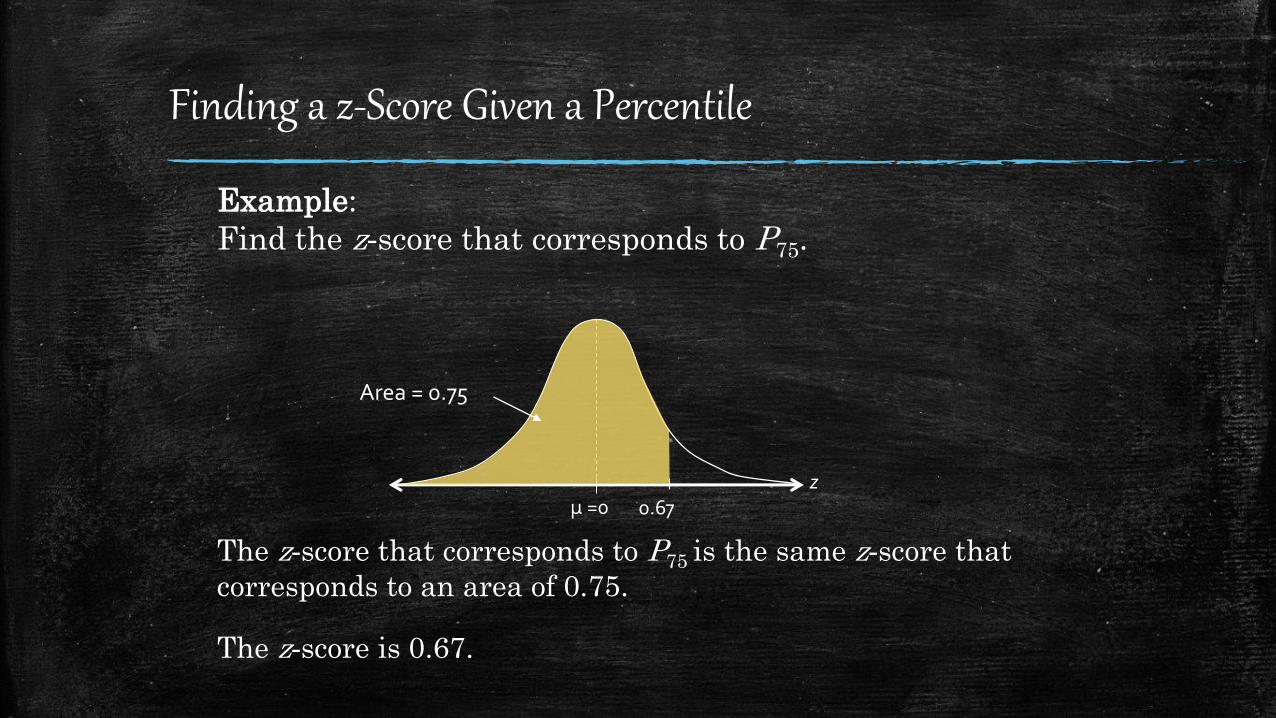
Finding a z-Score Given a Percentile
Example:
Find the z-score that corresponds to P75.
The z-score that corresponds to P75 is the same z-score that
corresponds to an area of 0.75.
The z-score is 0.67.
?μ =0z
0.67
Area = 0.75
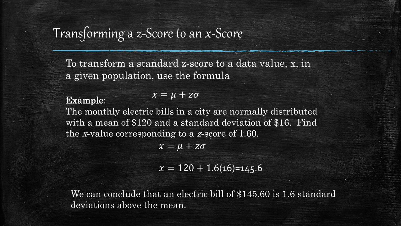
Transforming a z-Score to an x-Score
To transform a standard z-score to a data value, x, in
a given population, use the formula
Example:
The monthly electric bills in a city are normally distributed
with a mean of $120 and a standard deviation of $16. Find
the x-value corresponding to a z-score of 1.60.
We can conclude that an electric bill of $145.60 is 1.6 standard
deviations above the mean.
𝑥 = 𝜇 + 𝑧𝜎
𝑥 = 𝜇 + 𝑧𝜎
𝑥 = 120 + 1.6(16)=145.6
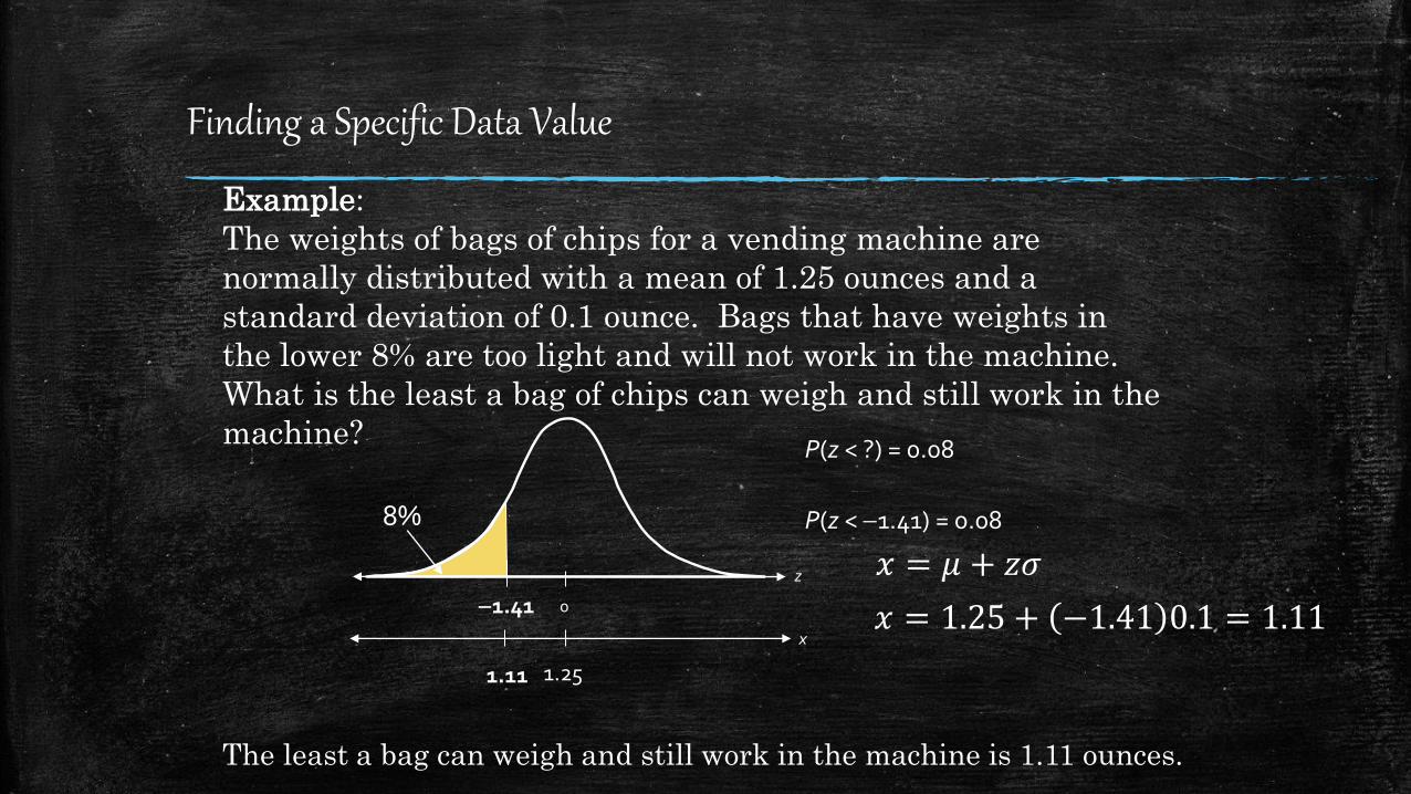
Finding a Specific Data Value
Example:
The weights of bags of chips for a vending machine are
normally distributed with a mean of 1.25 ounces and a
standard deviation of 0.1 ounce. Bags that have weights in
the lower 8% are too light and will not work in the machine.
What is the least a bag of chips can weigh and still work in the
machine?
The least a bag can weigh and still work in the machine is 1.11 ounces.
? 0
z
8%
P(z < ?) = 0.08
P(z < 1.41) = 0.08
1.41
1.25
x
?1.11
𝑥 = 𝜇 + 𝑧𝜎
𝑥 = 1.25 + −1.41 0.1 = 1.11
Recommended