REPORT NUMBER: WI/SPR-04-00
LAYER COEFFICIENTS FOR NEW AND REPROCESSED ASPHALTIC MIXES
FINAL REPORT
JANUARY 2000

Technical Report Documentation Page 1. Report No. 2. Government Accession No. 3. Recipients Catalog No. WI/SPR-04-00 4. Title and Subtitle 5. Report Date Layer Coefficients for New and Reprocessed Asphaltic Mixes January 2000 6. Performing Organization Code 7. Author(s) 8. Performing Organization Report No. H. U. Bahia, Assistant Professor; P. J. Bosscher, Professor; J. Christensen, Research Assistant; and Yu Hu, Research Assistant 9. Performing Organization Name and Address 10. Work Unit No. (TRAIS) University of Wisconsin - Madison Dept. of Civil and Environmental Engineering 1415 Engineering Drive 11. Contract or Grant No. Madison, WI 53706-1490 WisDOT SPR # 0092-45-86 12. Sponsoring Agency Name and Address 13. Type of Report and Period Covered Wisconsin Department of Transportation Final Report Division of Transportation Infrastructure Development Bureau of Highway Construction 14. Sponsoring Agency Code Pavements Section, Technology Advancement Unit WisDOT Study # 97-02 3502 Kinsman Blvd., Madison, WI 53704-2507 15. Supplementary Notes 16. Abstract
The objective of this study is to determine layer coefficients for selected types of asphalt mixtures used in Wisconsin including LV. MV, HV, SMA, SHRP, pulverize-Relay mixtures, Mill-Relay mixtures, asphalt base mixtures and recycled PCC-AC mixes combined at different percentages. The traditional method of resilient modulus was used as well as relating rutting damage functions to the layer coefficients. Tests were conducted in the field to measure deflections of actual pavement layers, as well as in the laboratory to measure the responses of samples under conditions that mimic field conditions. The results of the study show that laboratory and field measurements are consistent with the materials tested. The resilient modulus values measured show that different layer coefficients should be given to the recycled and reprocessed materials depending on the nature of the components. A list of layer coefficients is proposed for pavement design. The results of the asphalt materials did not show that there are significant differences in resilient modulus of asphalt mixtures tested; thus, layer coefficients for the asphalt mixtures, derived based on the resilient modulus, are similar for all asphalt mixtures. The results of laboratory rutting tests, however, were found to give different ranking of the materials, compared to the ranking using the resilient modulus results. It is observed that asphalt mixtures vary significantly in their rutting behavior in the laboratory and thus can have different contribution to pavement performance. It is recommended that proposed layer coefficients be used with caution due to lack of direct relation to materials damage behavior. A conceptual procedure for deriving layer coefficients based on resilient modulus, rutting behavior, and fatigue behavior is proposed in the study. The study recommends continued work to verify the proposed procedure and modify the layer coefficients to account for the damage behavior of pavement materials including fatigue and thermal cracking. 17. Key Words LAYER COEFFICIENTS, RESILIENT MODULUS, PAVEMENT DESIGN, RUTTING, FATIGUE, CRACKING
18. Distribution Statement
19. Security Classif. (of this report) 20. Security Classif. (of this page) 21. No. of Pages: 129 22. Price
i
LAYER COEFFICIENTS FOR NEW AND REPROCESSED ASPHALTIC MIXES
FINAL REPORT WI/SPR-04-00 WisDOT Highway Research Study # 97-02
By
H.U. Bahia, Assistant Professor P.J. Bosscher, Professor
J. Christensen, Research Assistant Yu Hu, Research Assistant
University of Wisconsin - Madison Department of Civil & Environmental Engineering 1415 Engineering Drive, Madison, WI 53706-1490
For
WISCONSIN DEPARTMENT OF TRANSPORTATION DIVISION OF TRANSPORTATION INFRASTRUCTURE DEVELOPMENT
BUREAU OF HIGHWAY CONSTRUCTION TECHNOLOGY ADVANCEMENT UNIT
3502 KINSMAN BLVD., MADISON, WI 53704-2507
January 2000
The Technology Advancement Unit of the Division of Transportation Infrastructure Development, Bureau of Highway Construction, conducts and manages the highway technology advancement program of the Wisconsin Department of Transportation. The Federal Highway Administration provides financial and technical assistance for these activities, including review and approval of publications. This publication does not endorse or approve any commercial product even though trade names may be cited, does not necessarily reflect official views or policies of the agency, and does not constitute a standard, specification or regulation.
ii
TABLE OF CONTENTS
TECHNICAL REPORT DOCUMENTATION PAGE……………………………………………….……...i
TITLE PAGE
………………………………………………………………………………………………….ii
TABLE OF CONTENTS
...…………………………………………………………………...………..……iii
LIST OF
FIGURES………………..………………………………………………………………………….v
LIST OF TABLES…………………………………………………………………………………………
.vi
CHAPTER ONE: INTRODUCTION … …………………………………………………………………..1
1.1 Background ……………………………………………………………………………………...1 1.2 Problem Statement …………………………………………………………………………….2 1.3 Research Objectives……………………………………………………………………………2 1.4 Research Methodology ………………………………………………………………………...3 1.5 Research Scope…………………………………………………………………………..…….4 1.6 Summary………………………………………………………………………………………...5
CHAPTER TWO: LITERATURE REVIEW6
2.2 Literature Review…………………………………………………………………………….6
2.2.1 Layer Coefficients…………………………………………………………………….6 2.2.1.1 Background of AASHTO Layer Coefficients ...……………………..……….6 ...... 2.2.1.2 Structural Layer Coefficients as Determined by Different Departments of Transportation in the U.S.…………………..…………………………10 .................................................................................................................................. 2.2.1.2.1 NCHRP Report No. 128.......................... ……………………………………….10 .................................................................................................................................. 2.2.1.2.2 1997 Survey of Midwestern States .......................... ………..…………………13 ............2.2.1.3 Using Probabilistic Fatigue Model to Determine Layer Coefficients..13 ......................... 2.2.1.4 Using Material Properties to Determine Layer Coefficients ……….…14 .................................................................................................................................. 2.2.1.4.1 Resilient Modulus.......................... ………………………………………………14 .................................................................................................................................. 2.2.1.4.2 Dynamic Shear Modulus.......................... ………………………………………18 .................................................................................................................................. 2.2.1.4.3 California Bearing Ratio (CBR)................................ …………………………..19 .................................................................................................................................. 2.2.1.4.4 Elastic Modulus of Base Layer ......................... ………………………………..21 .....................................................2.2.1.5 Wisconsin Department of Transportation ……………………………..22
iii
2.2.2 Background of Field Measurements……………………………………………24 .................................................... 2.2.2.1 The Falling Weight Deflectometer (FWD) ……………………………..24 .............................................. 2.2.2.2 The Use of the Falling Weight Deflectometer …………………………25 2.2.3 Permanent Deformation Damage Functions…………………………………..28 2.2.4 Rutting and Resilient Characteristics as Determined by Tri-Axial Testing….33
CHAPTER THREE: MATERIAL COLLECTION, SPECIMEN PREPARATION, DATA .................................................................. COLLECTION, AND CALCULATION......................................................................................... ……………………………………….40 ......................................................................................... 3.1 Material and Project Descriptions.................................................................…………………………………………………………40 .....................................................................................................................................................3.1.1 Bound Materials ..........................…………………..………………………………………………40 .....................................................................................................................................................3.1.2 Unbound Materials............................... ……………………………………………………………48 ........................................................................................3.2 Field Data Collection and Analysis................................................................... ………….……………………………………………53 .....................................................................................................................................................3.2.1 Field Data Collection......................... ………………………………………..….…………………53 .....................................................................................................................................................3.2.2 Field Data Backcalculation Methods.........................……………….……………………………53 .............................................................................. 3.3 Laboratory Data Collection and Analysis............................................................................. ..………………………………………………54 3.3.1 Specimen Preparation ………………………………….…………………………54 3.3.2 Testing Parameters …………………………………….…………………………56 3.3.2.1 Unbound Material Parameters …………………….……………………57 3.3.2.2 Asphalt Surface Course Parameters …………………………………58 3.3.3 Data Collection Methods …………………………………………………………60 3.3.4 Laboratory Data Transformation Techniques ………………..…………………61 3.3.4.1 Laboratory Resilient Modulus Calculations …………………….……..61 3.3.4.2 Permanent Deformation (Rutting) Calculations ………………………63
CHAPTER FOUR : FIELD TESTING RESULTS AND ANALYSIS …………………………64
4.1 Resilient Modulus Calculations……………….….…………………………………………..65 4.2 Field Testing Results ……………………………………………………………….………66 CHAPTER FIVE: LABORATORY RESULTS AND ANALYSIS ……….………………………….69
5.1 Repeatability Testing and Confining Pressure Control………………………….…...……69 5.2 Unbound Material Laboratory Results and Analysis ……………………………………71 5.2.1 Resilient Modulus Results ……………………….………………………………72
5.2.1.1 A Comparison of the Results of Different Materials ………………… ...74 5.2.1.2 Calculations of Layer Coefficients for Unbound Materials ………...…75
5.2.2 Permanent Deformation Results ……………………………………..…………76 5.2.2.1 Permanent Deformation Damage Functions ………………………….76 5.2.2.2 Comparison of Rutting Behavior………………………………...………...80
5.2.2.3 Deriving the a2 Values………………………………………….…………..81 5.3 Bound Material Results ……………………………………..……….…….…. 82 5.3.1 Resilient Modulus Results ……………………….…………………………….… 82 5.3.1.1 Comparisons of Bound Material Behaviors ………………………… 84 5.3.1.2 Resilient Modulus Layer Coefficients ………………………………… .84 5.3.2 Permanent Deformation Results for Asphalt Mixtures ………………………86 5.3.2.1 Permanent Deformation Damage Functions ………………………..88
iv
5.3.2.2 Temperature and Principle Stress Effects………………………….….…..92 5.3.2.3 Layer Coefficients and Permanent Deformation Comparisons ……92 5.3.2.4 Other Trends and Comparisons ………………………………………93
5.4 Derivation of New Layer Coefficients ……………………………………………………..94
CHAPTER SIX: FINDINGS AND FUTURE RECOMMENDATIONS ……………….……99
6.1 Summary of Findings …………………………………………………………………..99 Laboratory versus Field Measurements ……………………………………………99 Results of Unbound Reprocessed Materials …………………………………99 Results of Asphalt Mixtures …………………………..100 6.2 Conclusions and Recommendations ……………..……………………………101
REFERENCES ………………………………………………………………………………………..102
APPENDIX A- Survey Results of Midwestern States
…………………..………………......……..106
APPENDIX B- Tables of Testing Results
…………………………………………………….…..…..112
APPENDIX C- Asphalt Testing Results
………………………………………………..……………..117
APPENDIX D- Telfon Compliance……………………………………………………………...…..…122
APPENDIX E-High Temperature Resilient Modulus Results
………………………………….....126
LIST OF FIGURES
Figure 2.1 Determination of the stress p*………………………………………………………………... 39Figure 3.1 Recycled Material Gradation Curves …………………………………………………………
50
Figure 3.2 50-50 Modified Proctor Curve……………………………………………………………….. 50Figure 3.3 Pulverize Modified Proctor Curve……………………………………………………………. 51Figure 3.4 90P-10A Modified Proctor Curve……………..……………………………………………… 51Figure 3.5 70P-30A Modified Proctor Curve…………………………………………………………….. 52Figure 3.6 50P-50A Modified Proctor Curve ……………………………………………………………. 52Figure 3.7 Density Profiles of Compacted Asphalt Mixes …………………………………….….……. 56Figure 3.8 Schematic Diagram of a Tri-Axial Cell ……………………………………………….………
61
Figure 3.9 An Example of a Test Data File Generated by the Tri-Axial Testing Equipment ………. 62Figure 4.1 Deflection from MV Section Subbase ……………………………………………….……….
64
Figure 4.2 Deflection from MV Section AC Surface ……………………………………………..……...
65
Figure 4.3 The Backcalculated Mr Results from the MV Section ……………………………….…….. 67Figure 4.4 The Backcalculated Mr Results from the SHRP Section ………………………………….. 67Figure 4.5 The Backcalculated Mr Results from the ABC Section ……………………………………. 68
v
vi
Figure 5.1 50-50 M Br B Trials Showing Test Repeatability …………………………………………... ….. 70Figure 5.2 SHRP Rutting Repeatability – Confining Pressure Applied ………………………………. 71Figure 5.3 Pulverize with 13% Shoulder Aggregate – Dry M Br B Test Results …………………………. 73Figure 5.4 Final M Br B Test Results for the Granular Base Course Materials …………………………...
73
Figure 5.5 Layer Coefficients Estimated for Unbound Material …………..………………………….. 75Figure 5.6 Rutting Results of unbound materials at the stress condition of 103kPa σ B3B – 103kPa σ Bd B ……………………………………………………………………… 77Figure 5.7 Rutting Results for the 50-50 Material at Different Moisture and Stress Conditions…….
77
Figure 5.8 Strain Intercepts for Unbound Materials ……………………………………………………. 78Figure 5.9 Line Slope Values for Unbound Materials………………………………………….……….. 78Figure 5.10 Load Repetitions Required to Reach 0.3% Strain for Granular Materials ………………. 79Figure 5.11 Results of Testing the HV Mixture for Mr at 20°C …………………………………………. 83Figure 5.12 Asphalt Material M Br B Results @ 20°C ………………………………………………………... 83Figure 5.13 Layer Coefficients of Asphalt Mixtures Estimated for 2 Depths to Represent a Surface and a Binder Layer ………………………………….………………………………. 86Figure 5.14 Rutting Results for the SHRP Mixture at Different Combinations of Stresses and Temperatures ……….………………………………………………………….……………... 87Figure 5.15 Figure 5.15 Rutting Tests Results at a σ B3B of 103kPa, σ BdB of 450kPa, and a Temperature of 64°C ………………………………………………………………………….. 88Figure 5.16 Strain Intercepts from Logarithmic Linear Relationships ……………..………….……….. 89Figure 5.17 Line Slope Values from Logarithmic Linear Relationships ..……………………………… 90Figure 5.18 Asphalt Surface Mixtures Rutting Performance ……………………..…..…………… …... 91Figure 5.19 103-310-52-Dry Rutting Results for All Materials ……………………..…………………… 94
LIST OF TABLES
Table 1.1 Layer Coefficient Material and Project Table…………………………………………
4
Table 2.1 The Results of the 1972 AASHTO Survey of Layer Coefficients……………...
11-12
Table 2.2 Stress Levels For Permanent Deformation Tests……………………………………
37
Table 3.1 Materials Analyzed for Layer Coefficient Project……………………………………. 41Table 3.2 SHRP Mixture Properties……………………………………………………………… 42Table 3.3 SMA Mixture Properties……………………………………………………………….. 43Table 3.4 HV-2 Mixture Properties……………………………………………………………….. 45Table 3.5 MV-2 Mixture Properties……………………………………………………………….. 46Table 3.6 ABC Mixture Properties…………………………………………………………………
47
Table 3.7 Recycled Material 49
Gradations…………………………………………………………. Table 3.8 Asphalt Material Compaction Specifications………………………………………… 55Table 3.9 Laboratory Testing Parameters……………………………………………………….. 60Table 3.10 Testing Sequence for Type 1 Soils………………………………………………….. 63Table 4.1 Summary of Mr and aI Estimated from FWD Results……………………………….. 66Table 4.2 Section Layer Thicknesses……………………………………………………………. 66Table 5.1 Base Material Mr and a2 Values………………………………………………………. 74Table 5.2 Base Material a2 values and N0.003 Results………………………………………….. 80Table 5.3 Asphalt Mixture a1 and Mr Values…………………………………………………….. 85Table 5.4 Asphalt Surface Material a2 Values and N0.01 Results……………………………… 93
vii
CHAPTER ONE
INTRODUCTION
1.1 Background
In the late 1950’s and early 1960’s, the American Association of State Highway Officials
(AASHO) conducted a limited road test, the purpose of which was to determine a methodology for
designing pavement structures. This organization, which later became the American Association of State
Highway and Transportation Officials (AASHTO) used the AASHO Road Test results to introduce the
1972 AASHTO Asphalt Pavement Design Guide.
The AASHTO Guide methodology is based on using an abstract number that solved design
equations called structural numbers (SNs). A SN expresses the structural capacity of the pavement
structure required for given combinations of a total equivalent to 18-kip single axle loads (EASLs), soil
support values, terminal serviceability indexes, and regional factors. This method is based on the
pavement performance-serviceability concept developed during the AASHO Road Test. The method,
which was updated in 1986 and 1993, utilizes layer coefficients (ai values) to integrate a pavement
structure using materials of varied supporting capacities. The SN combines the impacts of the layer
coefficients, layer thicknesses, and drainage coefficients on the pavement structure.
The original layer coefficients were regression coefficients developed by relating layer thickness
to a road performance determined on basis of the parameters of the AASHO Road Test. The
development of the layer coefficients has been evolving; the most recent AASHTO Design Guide,
published in 1993, stipulates that layer coefficients can vary depending on a number of factors. These
factors include material type, material properties, type of layer, traffic level, and failure criterion. The
principle variables are material types and material properties. Material types vary everywhere across the
country and the material properties are dependent on construction practices and local environments.
These conditions as well as traffic levels exhibit a wide range across the country. Therefore, the layer
coefficients given in the AASHTO Design Guide are expected to be used universally, whereas different
layer coefficients are expected to be developed for local conditions.
1

The 1993 AASHTO Design Guide recommends using the resilient modulus as the standard
material quality measure to account for material types and material properties. Also, layer coefficients are
still identified according to their treatment in the structural number design approach. In other words, a
material with a certain resilient modulus will receive a lower layer coefficient if it is used as a base rather
than a sub-base.
1.2 Problem Statement
Asphalt has advanced since the time of the original AASHO Road Test and the publication of the
1972 AASHTO Design Guide. In the 1980’s, many states, including Wisconsin, started to change the
specifications for Asphalt Concrete (AC) mix designs. More durable pavements were needed to support
the ever-increasing traffic loads. Recently -in the 1990’s- the use of reprocessed asphalt pavements as
base courses has become more widely used.
Even though mix design and material types have evolved and changed, the layer coefficients for
asphalt pavements have not been studied or revised to accommodate these changes in technology.
Wisconsin, like many other states, does not differentiate between different types of AC surface mixes and
base courses.
1.3 Research Objectives
The main objective of this research is to evaluate some of the new mixtures and materials using
laboratory and field measures to determine if the layer coefficients need to be updated and differentiated
for new and reprocessed materials.
To achieve this objective, the research is supposed to include actual pavement damage
indicators in the calculation of the layer coefficients. During the last few years some research has
suggested that using the resilient modulus alone for the calculation of a layer coefficient is not sufficient.
Actual pavement damage, such as permanent deformation (rutting) and fatigue cracking, must be taken
into account in order to formulate a layer coefficient that will reflect actual pavement behavior.
2
These goals will not only lead to updated layer coefficients, but also to the development of a more
reliable method that will include pavement-rutting characteristics and other types of failure in the
formulation of those layer coefficients. This approach can be used to evaluate new pavement and base
course materials that are developed in the future.
1.4 Research Methodology
The methodology for this research starts with a literature review with a view to clarifying how the
layer coefficients were derived, how they were calculated using resilient modulus, and how resilient
modulus was determined. The literature review also sheds light on other material properties used to
determine layer coefficients. The use of the Falling Weight Deflectometer (FWD) to determine resilient
moduli and the concepts behind the method were also reviewed. In order to prepare for the testing in this
project, the literature review was extended to include the development of tri-axial cells used to test
granular materials and asphalt mixtures.
Material types were chosen to cover traditional mixture designs and two mix designs that
represented more recent technologies (SHRP & SMA). Two types of recycled base courses were also
included. The materials were collected from construction projects from different parts of Wisconsin.
Field measurements using the FWD were conducted at certain locations investigate how they
would compare to compare with laboratory results. The laboratory results were generated using a tri-axial
apparatus. Both resilient modulus and rutting tests were performed on all materials. Due to time and
equipment limitations, fatigue cracking was not considered in this research plan.
Field data was processed using backcalculation techniques to determine resilient moduli. The
laboratory resilient modulus data was analyzed using parameters developed for the testing of granular
materials. The rutting data was analyzed by comparing cumulative strains to number of load repetitions.
The field data was compared to laboratory data to validate the laboratory results. Finally,
recommendations for future analysis, possible test method improvements, and suggestions for future
research are presented.
3
1.5 Research Scope
To investigate the possibility of an improved method for estimating layer coefficients and possible
relations between rutting and layer coefficients, several materials were tested using both field and
laboratory methods. Field measurements were conducted with the use of the FWD. For certain sections
each layer of the pavements was tested as they were being constructed. Materials from all the sites
where field-testing took place were collected for laboratory testing.
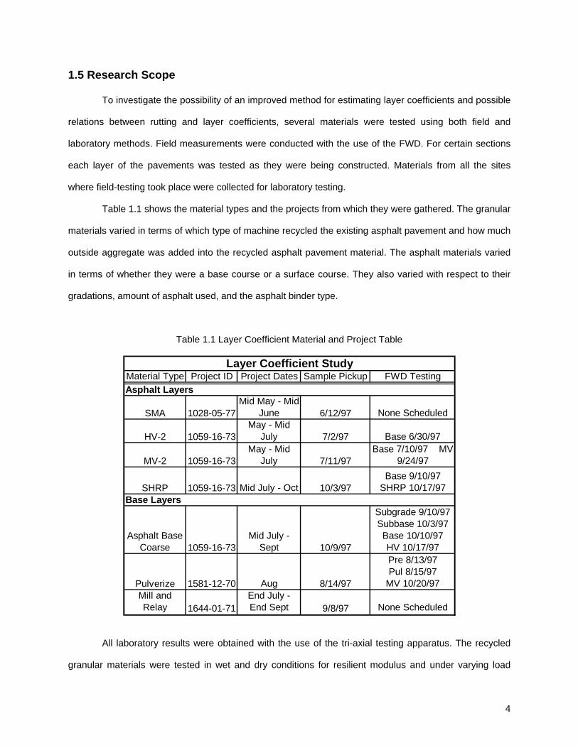
Table 1.1 shows the material types and the projects from which they were gathered. The granular
materials varied in terms of which type of machine recycled the existing asphalt pavement and how much
outside aggregate was added into the recycled asphalt pavement material. The asphalt materials varied
in terms of whether they were a base course or a surface course. They also varied with respect to their
gradations, amount of asphalt used, and the asphalt binder type.
Table 1.1 Layer Coefficient Material and Project Table
Material Type Project ID Project Dates Sample Pickup FWD TestingAsphalt Layers
SMA 1028-05-77Mid May - Mid
June 6/12/97 None Scheduled
HV-2 1059-16-73May - Mid
July 7/2/97 Base 6/30/97
MV-2 1059-16-73May - Mid
July 7/11/97Base 7/10/97 MV
9/24/97
SHRP 1059-16-73 Mid July - Oct 10/3/97Base 9/10/97
SHRP 10/17/97Base Layers
Asphalt Base Coarse 1059-16-73
Mid July - Sept 10/9/97
Subgrade 9/10/97 Subbase 10/3/97 Base 10/10/97 HV 10/17/97
Pulverize 1581-12-70 Aug 8/14/97
Pre 8/13/97 Pul 8/15/97
MV 10/20/97Mill and Relay 1644-01-71
End July - End Sept 9/8/97 None Scheduled
Layer Coefficient Study
All laboratory results were obtained with the use of the tri-axial testing apparatus. The recycled
granular materials were tested in wet and dry conditions for resilient modulus and under varying load
4

5
conditions for rutting. The asphalt materials were tested at 52°C and 64°C for resilient modulus and under
varying load conditions for rutting.
The scope of the analysis in this report is limited to the analysis of the data collected from the
above-mentioned field and laboratory tests. The first part covers the resilient modulus testing and the
comparison between field and laboratory data. The second part covers the rutting results and how these
can be formulated into damage functions.
1.6 Summary
This report is divided into seven chapters. The first chapter provides an introduction, objectives,
methodology, scope, and summary of the research. In chapter 2, a literature review investigating the
background of layer coefficients, resilient modulus, FWD methods, permanent deformation damage
functions, and tri-axial test apparatus is presented. Chapter 3 describes both the field and laboratory data
collection methods, including how the laboratory specimens were manufactured. Field data results and
analyses are presented in Chapter 4. The laboratory results and analyses are discussed in the following
chapter. Finally, the research findings and future recommendations are summarized in Chapter 6.
CHAPTER TWO
LITERATURE REVIEW
2.1 Introduction
The AASHO Road Test was developed in the late 1950’s to provide information that could be
used to develop pavement design criteria and procedures. When completed, the road test directly lead to
the 1961 AASHO Interim Guide for the Design of Rigid and Flexible Pavements. This guide was modified
in the following decade and published in 1972 as the AASHTO Interim Guide for Design of Pavement
Structures – 1972. After that, major revisions to the guide were completed in 1986 and 1993.
The guide uses the concept of layer coefficients for asphalt pavements; these coefficients are
based on research conducted on a number of pavement and material properties. The coefficients are
indicators of the relative ability of a material to function as a structural component within the asphalt
pavement.
According to the AASHTO 1986 Guide the resilient modulus of a material is the primary means of
determining the layer coefficient of that material. However, there have been investigations that involved
other material properties to determine layer coefficients. Over the past few years, some people have
come to the conclusion that resilient modulus and strength are not enough to effectively gauge a
material’s behavior in a pavement structure. The literature review considers efforts put forth by
researchers to model permanent deformation in asphalt pavements.
Finally, types of tri-axial cells developed by different researchers are reviewed in an effort to learn
from their experiences. The tri-axial cell was the critical part of the entire laboratory testing. Therefore, an
understanding of how this type of apparatus is set up was crucial.
2.2 Literature Review
2.2.1 Layer Coefficients
2.2.1.1 Background of AASHTO Layer Coefficients
The solution to the design equations in the different versions of the AASHTO pavement design
6

7
guide is in terms of a structural number (SN). The structural number is an abstract number expressing
the structural strength of pavement required for a given combination of soil support value, total equivalent
18-kip (80 kN), single axle loads (ESALs), terminal serviceability index, and regional factor. The
magnitude of the SN reflects the degree to which the sub-grade must be protected from the effects of
traffic. The AASHTO Guide for the Design of Pavement Structures, based on the pavement performance-
serviceability concept developed from the AASHO Road Test, utilized the concept of “layer coefficients”
(a Bi B values) to synthesize a pavement structure employing materials of varied supporting capacities.
A value for this coefficient is assigned to each layer material in the pavement structure in order to
convert actual layer thickness into structural numbers (SN). This layer coefficient expresses the empirical
relationship between SN and thickness; it is a measure of the relative ability of the material to function as
a structural component of the asphalt pavement.
The following general equation for the structural number reflects the relative impact of the layer
coefficients (a Bi B), thickness (D Bi B), and the drainage coefficients (mBi B) on the structural number:
iii mDamDamDaDaSN ++++= ...33322211 (1)
The AASHTO guide proposed numerical values for the structural layer coefficient of materials, a-
values, which were originally regression coefficients that resulted from relating layer thickness to road
performance under the conditions of the road test.
According to the most recent AASHTO guide (1993), the a-value can vary considerably depending
upon a number of factors. These involve:
1. layer thickness
2. material type
3. material properties
4. layer location (base, sub-base)
5. traffic level
6. failure criterion
Material type and properties are the principle variables that affect the layer coefficient. In addition,
material properties are dependent on environment and construction practices. Because of the wide
variations in environments, traffic, and construction practices, the proposed a-values in the AASHTO

guide are not expected to apply to all cases. As a result, different a-values should be determined based
on local conditions.
To account for material type and properties in the 1993 AASHTO guide, the elastic (resilient)
modulus (Mr) is used as the standard material quality measure. It is still necessary to identify the
corresponding layer coefficients because of their treatment in the SN design approach. For example, a
granular material with a certain modulus will get a lower layer coefficient if used as a base course
material than if used as a sub-base.
The relationship between the layer coefficients and the resilient modulus has been investigated in
several research efforts. The layer coefficient does not only reflect the stress distribution in the layer, but
is also an index of the strength of the material. The position of the material in the structure and the mode
of distress may, therefore, influence the relation between the layer coefficient and the resilient modulus.
Other investigators have used another parameter, the layer thickness equivalency, mainly for the
purpose of evaluating the support capacity of a given material compared to standard or commonly used
materials. The layer thickness equivalency is determined as the thickness of the material in question
required to replace 25 mm (1 inch) of the standard material (Mustaque et al. 1997).
Most of the methods used to evaluate either the layer coefficient or the layer thickness equivalency
are based on the evaluation of limiting criteria at specific points in the pavement structure. To establish
layer coefficients for the 1986 version of the AASHTO guide under various conditions and materials, three
criteria based on the mechanistic response to loads were evaluated:
1. surface deflection,
2. tensile strain in the asphalt layer, and
3. vertical compressive strain on the roadbed soil.
To establish the relationship between the layer coefficient and the resilient modulus, a range of
surface thicknesses (D1) and base thicknesses (D2) were used to calculate deflection, tensile strain, and
vertical compressive strain. The results were used to evaluate the required increase in base thickness for
a decrease in surface thickness while holding the deflection or strain level constant.
8

9
Layer coefficient values for different layers made of different materials can be determined using
empirical equations derived from field experiments. The following equations are some of the commonly
used relationships (Mustaque et al. 1997):
Asphalt concrete:
aEMPa
a1 10 43000
0 44 0 20 0 44= ×⎛
⎝⎜
⎞
⎠⎟ + < <. log . . . (2)
Bituminous-treated Base:
3.01.015.03000
log*3.0 22 <<+⎟⎠⎞
⎜⎝⎛= a
MPaEa (3)
Granular Subbase:
2.006.015.0160
log*23.0 33 <<+⎟⎠⎞
⎜⎝⎛= a
MPaEa (4)
In the AASHTO design procedure a number of relationships have been derived using layered
elastic theory to evaluate a combination of pavement cross-sections and material properties. In addition
to the following relationships, charts for estimation were developed for other materials:
Granular Base:
aB2B = 0.249 log E2 – 0.977 ( 4a )
Granular Subbase:
a B3B = 0.227 log E3 –0.839 ( 4b )
Where a Bi B values are the layer coefficients and the EBi B values are the resilient modulus values.
The relationship between layer coefficients and resilient moduli is generally based on layered elastic
theory. Layer coefficients are affected by more factors than just material stiffness and strength, which is

why these empirical relationships are derived. Appendix G in the 1993 AASHTO guide provides values
for a1 as a function of the properties of the selected materials.
2.2.1.2 Structural Layer Coefficients as Determined by Different Departments of Transportation in the
U.S.
2.2.1.2.1 NCHRP Report No. 128
As part of the National Cooperative Highway Research Program (NCHRP) project (McCullough
1972) a survey of state highway agencies was conducted to collect information regarding the layer
coefficients to be used in the AASHTO design method. Table 2.1 summarizes the results of that survey.
For a given layer, it appears that in most cases values for the layer coefficient have been associated only
with a material description.
The Asphalt Institute also conducted a study to develop layer coefficients for asphalt layers.On
the basis of that research, it was concluded that the structural components (surfacing, base, and sub-
base) could be treated as linear combinations of equivalent thicknesses of each layer. That is:
D = a1D1 + a2D2 + a3D3. (5)
The Asphalt Institute method for determining equivalency factors was based on the AASHTO
Road Test survey of prior performance, together with theoretical considerations. The AASHTO Road Test
Report 61-E included a development of structural coefficients based on Performance Serviceability Index,
cracking, and deflection. Three separate multiple linear regression analyses were performed on the
AASHTO road test data. On the basis of the analysis presented in the report, it was concluded that
asphalt concrete can be 2 to 6 times more effective than good crushed stone.
10
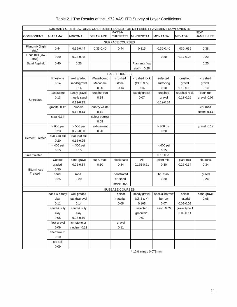
Table 2.1 The Results of the 1972 AASHTO Survey of Layer Coefficients
COMPONENT ALABAMA ARIZONA DELAWAREMASSA-CHUSETTS MINNESOTA MONTANA NEVADA
NEW HAMPSHIRE
Plant mix (high stab) 0.44 0.35-0.44 0.35-0.40 0.44 0.315 0.30-0.40 .030-.035 0.38
Road mix (low stab) 0.20 0.25-0.38 0.20 0.17-0.25 0.20
Sand Asphalt 0.40 0.25 Plant mix (low 0.20stab) 0.28
limestone well graded Waterbound crushed crushed rock selected crushed crushed0.14 sand&gravel Macadam stone (Cl. 5 & 6) surfacing gravel gravel
0.14 0.20 0.14 0.14 0.10 0.10-0.12 0.10sandstone sandy gravel, crusher run sandy gravel crushed crushed rock bank run
0.13 mostly sand 0.14 0.07 gravel 0.13-0.16 gravel 0.070.11-0.13 0.12-0.14
granite 0.12 cinders quarry waste crushed0.12-0.14 0.11 stone 0.14
slag 0.14 select borrow0.08
> 650 psi > 500 psi soil-cement > 400 psi gravel 0.170.23 0.25-0.30 0.20 0.20
400-650 psi 300-500 psi0.20 0.18-0.25
< 400 psi < 300 psi < 400 psi0.15 0.15 0.15
Lime Treated 0.15-0.20Coarse sand-gravel asph. stab. black base All plant mix plant mix bit. conc.graded 0.25-0.34 0.10 0.34 0.175-0.21 0.30 0.25-0.34 0.34
0.30sand sand penetrated bit. stab. gravel0.25 0.20 crushed 0.20 0.24
stone .029
sand & sandy well graded select sandy gravel special borrow select sand-gravelclay sand&gravel material (Cl. 3 & 4) borrow material 0.050.11 0.14 0.08 0.105 0.07 0.05-0.09
sand & silty sand & silty selected sand 0.05 gravel type 1clay clay granular* 0.09-0.110.05 0.05-0.10 0.07
float gravel cr. stone or gravel0.09 cinders 0.12 0.11
chert low PI0.10
top soil0.09
* 12% minus 0.075mm
Cement Treated
SUBBASE COURSES
Bituminous Treated
SUMMARY OF STRUCTURAL COEFFICIENTS USED FOR DIFFERENT PAVEMENT COMPONENTS
SURFACE COURSES
BASE COURSES
Untreated
11
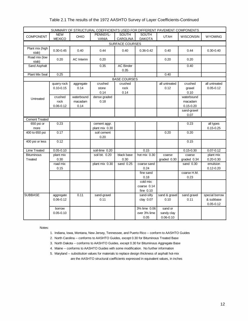
Table 2.1 The results of the 1972 AASHTO Survey of Layer Coefficients-Continued
COMPONENT NEW MEXICO OHIO PENNSYL-
VANIASOUTH
CAROLINASOUTH
DAKOTA UTAH WISCONSIN WYOMING
Plant mix (high stab) 0.30-0.45 0.40 0.44 0.40 0.36-0.42 0.40 0.44 0.30-0.40
Road mix (low stab)
0.20 AC Interim 0.20 0.20 0.20
Sand Asphalt 0.35 AC Binder 0.400.35
Plant Mix Seal 0.25 0.40
quarry rock aggregate crushed crushed all untreated crushed all untreated0.10-0.15 0.14 stone rock 0.12 gravel 0.05-0.12
0.14 0.14 0.10crushed waterbound dense graded waterbound
rock macadam 0.18 macadam0.06-0.12 0.14 0.15-0.20
sand-gravel0.07
650 psi or 0.23 cement aggr. 0.23 all typesmore plant mix 0.30 0.15-0.25
400 to 650 psi 0.17 soil cement 0.20 0.200.20
400 psi or less 0.12 0.15
Lime Treated 0.05-0.10 soil-lime 0.20 0.15 0.15-0.30 0.07-0.12 Bituminous plant mix soil bit. 0.20 black base hot mix 0.30 coarse coarse plant mix Treated 0.30 0.30 graded 0.30 graded 0.34 0.20-0.30
road mix plant mix 0.30 sand 0.25 coarse sand sand 0.30 emulsion0.15 0.24 0.12-0.20
fine sand coarse H.M.0.18 0.23
cold mix:coarse 0.14
fine 0.10SUBBASE aggregate 0.11 sand-gravel sand-silty sand & gravel sand gravel special borrow
0.06-0.12 0.11 clay 0.07 0.10 0.11 & subbase0.05-0.12
borrow 3% lime 0.06 sand or0.05-0.10 over 3% lime sandy clay
0.05 0.06-0.10
Notes:1. Indiana, Iowa, Montana, New Jersey, Tennessee, and Puerto Rico -- conform to AASHTO Guides2. North Carolina -- conforms to AASHTO Guides, except 0.30 for Bituminous Treated Base3. North Dakota -- conforms to AASHTO Guides, except 0.30 for Bituminous Aggregate Base4. Maine -- conforms to AASHTO Guides with some modification. No further information5. Maryland -- substitution values for materials to replace design thickness of asphalt hot-mix
are the AASHTO structural coefficients expressed in equivalent values, in inches
Cement Treated
SUMMARY OF STRUCTURAL COEFFICIENTS USED FOR DIFFERENT PAVEMENT COMPONENTS
SURFACE COURSES
BASE COURSES
Untreated
12

13
It was found that 25.4 mm (1 in) of high-quality asphalt concrete surfacing would be equivalent to 50.8
mm (2 in) to 76.2 mm (3 in) of good dense-graded, crushed-stone base, and that 25.4 mm (1 in) of
asphalt concrete base would be approximately equivalent to 50.8 mm (2 in) of such crushed stone. The
Asphalt Institute decided on an equivalency factor of at least 2 to 1 for asphalt concrete surface or base
to aggregate base and 2.67 to 1 for asphalt concrete surface or base to aggregate sub-base.
2.2.1.2.2 1997 Survey of Midwestern States
As part of the literature review for this project, a survey of State Departments of Transportation
(DOT’s) in the Midwest area was conducted. The survey focused on design methods and layer
coefficients used in the design procedure. The states included were: Illinois, Indiana, Iowa, Kansas,
Kentucky, Michigan, Minnesota, Missouri, Nebraska, North Dakota, Ohio, and South Dakota. Responses
were received from all states that were contacted.
The results from the states varied depending on the research and layer coefficients involved.
However, all of the states contacted used one form or another of the AASHTO design method. Illinois and
Kentucky have switched to mechanistic design methods. These are methods that do not depend on any
observed performance characteristics; they rely solely on design theory. Appendix A shows a summary of
the contacts from the states and the design method that they use. It also shows the layer coefficients
used by each state. There is a wide variation in how many layer coefficients they assign and how they
identify materials. Most of the states, however, use a layer coefficient for AC of 0.4 or 0.44.
2.2.1.3 Using Probabilistic Fatigue Model to Determine Layer Coefficients
A new method for determining the layer coefficient of flexible pavement materials, using a pavement
model, was developed by George (1984). According to this method, the material properties associated
with the layer coefficient are:
1. Elastic constants (resilient modulus and Poisson's ratio), and
2. Fatigue susceptibility expressed in the ε-N diagram.
Layer coefficients of several pavement materials used widely in the State of Mississippi (asphalt
concrete, soil-cement, and soil-lime) were developed in this research. The task of developing layer
coefficients was accomplished in two steps. The first step was to relate fatigue performance of asphalt
mixes to the structural numbers based on a large database. The relationship (model) also included load,
temperature, and sub-grade support values as independent variables. In the second step, this model
was used to establish an “equivalence” between pavement materials and layer coefficients.
The primary purpose of the model is to predict the load applications that the pavement/sub-grade
system can withstand and still provide minimum acceptable serviceability. Although the authors
recognized that the three specific distress modes commonly considered in evaluating pavement
performance are fatigue cracking, permanent deformation (rutting), and low-temperature cracking, they
cite previous research which concluded that the most prevalent type of pavement distress in the United
States is fatigue cracking.
The layer coefficient calculation using this model is based on the premise that it is possible to
establish what is known as “thickness equivalency” between layers. The layer coefficient of soil-cement
base, for example, is computed by comparing its fatigue life with that of the asphalt base.
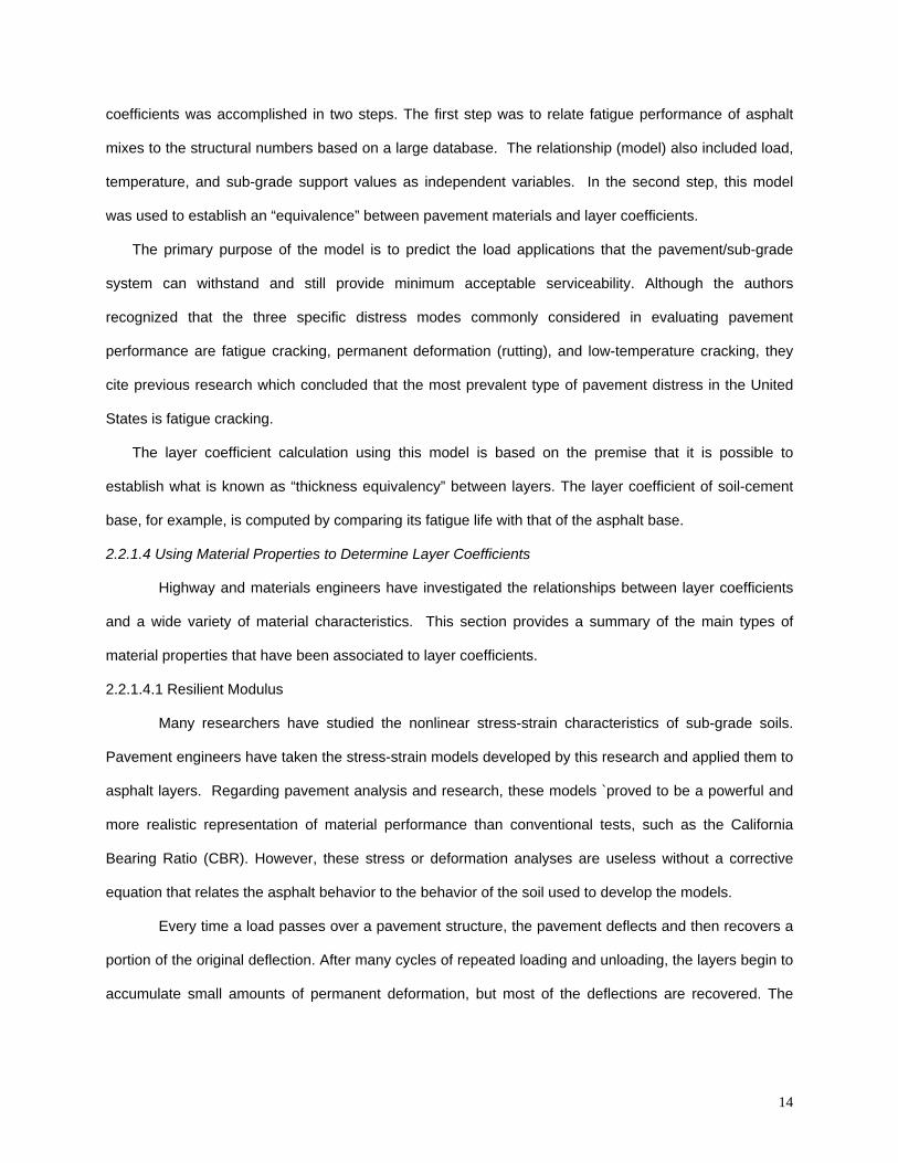
2.2.1.4 Using Material Properties to Determine Layer Coefficients
Highway and materials engineers have investigated the relationships between layer coefficients
and a wide variety of material characteristics. This section provides a summary of the main types of
material properties that have been associated to layer coefficients.
2.2.1.4.1 Resilient Modulus
Many researchers have studied the nonlinear stress-strain characteristics of sub-grade soils.
Pavement engineers have taken the stress-strain models developed by this research and applied them to
asphalt layers. Regarding pavement analysis and research, these models `proved to be a powerful and
more realistic representation of material performance than conventional tests, such as the California
Bearing Ratio (CBR). However, these stress or deformation analyses are useless without a corrective
equation that relates the asphalt behavior to the behavior of the soil used to develop the models.
Every time a load passes over a pavement structure, the pavement deflects and then recovers a
portion of the original deflection. After many cycles of repeated loading and unloading, the layers begin to
accumulate small amounts of permanent deformation, but most of the deflections are recovered. The
14
15
recovered deflections are termed resilient deformations. The resilient modulus (M BR B), which was
developed to explain this behavior, can be defined as:
R
dRM
εσ
= (6)
where
MBR B = resilient modulus
σ BdB = repeated deviator stress (σ B1B - σ B3B)
εBR B = recoverable axial strain in the direction of the principal stress σ B1B
Many research studies have been conducted to investigate the sensitivity of various factors
affecting resilient modulus. These factors include material type, sample preparation method, stress state,
the strain sensitivity of the material, and the condition of the samples (George & Uddin, 1994). Chen and
his co-researchers (1995) discussed the factors affecting the measurement of MBR B.
The procedure for determining MBR B has not yet been standardized. However, guidelines are given
in several AASHTO test methods (T274-82, T292-91I, and T294-92I). Different testing procedures may
result in different MBR B values ; hence, differences in the design of the pavement. Therefore, it is very
important to investigate the effects of pertinent factors on MBR Band the variability of MBR B values due to
different testing procedures. Although both the 1986 and 1993 AASHTO pavement design guides
emphasize the use of MBR B as a basis for material characterization, the procedures recommend the use of
a correlation between the modulus and the structure layer coefficients.
The results of several tests performed by the authors indicate that the greatest range of
differences between backcalculated and laboratory-determined moduli are for the asphalt concrete
layers, followed by the base and subgrade materials. They explained that these large
differences between backcalculated and laboratory AC moduli are a result of the existing cracks in the
pavement system.
The K-θ model, which is most commonly used in pavement design, reflects the stress
dependency behavior of granular materials. It is recommended for describing the nonlinear
characteristics of noncohesive or granular materials. The model is as follows:

16
M KRK= 1
2θ ( 7)
where
KB1B and KB2B = material constants, and
θ = bulk stress
While this model is good for representing the measured shear strain for calculating the elastic stiffness, it
may provide a very poor prediction of volumetric strain. Uzan (1985) suggested an improved M BR B model
that included the effect of shear stress. The new model is as follows:
M KRK
dK= 3
4 5θ σ (8)
where
KB3B, KB4B, and KB5B are material constants evaluated by a multiple regression analysis from a set of
repeated load MBR B tests and σ BdB is the deviator stress.
Witczak and Uzan (1988) suggested replacing the deviator stress σ BdB with the octahedral B Bshear
stress (τ BoctB ) as shown in the following equation. The bulk stress (θ) and the octahedral B Bshear stress were
normalized using atmospheric pressure (PBaB).
M K PP PR a
a
Koct
a
K
=⎡
⎣⎢
⎤
⎦⎥
⎡
⎣⎢
⎤
⎦⎥6
7 8θ τ (9)
where KB6B, KB7B, and KB8B are the material constants. The variable τ BoctB is given by:
( ) ( ) ( )[ ]τ σ σ σ σ σ σoct = − + − + −19 1 2
2
2 3
2
3 1
2 (10)
For tests performed under isotropic confining pressure, Eq. 11 can be simplified by using the
relationships σ B2B=σ B3B and σ B1B-σ B3B=σ BdB .
τ σoct d=2
3 ( 11 )
Some design methods use the typical stiffness values for granular materials ignoring the stress-
dependent aspect of behavior. The values are generally in the range of 100 to 300 MPa depending on
17
the aggregate type and its moisture condition (the moisture condition is dependent on the time of the
year). Chen et al. (1995) suggested two relationships between KB1B and KB2B based on different test
procedures. They are as follows:
log . .K K1 24 7308 2 5179= − , from T294-92I, and ( 12 )
log . .K K1 2419 17304= − , from T292-91I. (13)
Rada and Witczak (1981) investigated the feasibility of developing predictive MBR B equations from
physical properties of granular materials. They tried to develop a comprehensive evaluation of factors
that affect the MBR B response of granular materials. They analyzed six different aggregate types, for each
of which three hand-blended gradations were used. On each aggregate-gradation combination, three
compaction energies were used to develop moisture-density relations. The combined number of
individual granular material results used in the report was 271. The results of the research show that
there exist a relationship between the MBR B and the physical properties of the granular materials do exist.
Rada and Witczak (1981) found that each class of aggregates has its relatively unique KB1B-KB2B
relation that distinguishes it from the other groups. In addition, the overall mean values for all granular
materials is KB1B=9240 and KB2B=0.52. The largest variation of KB1B and KB2B is observed for the crushed stone
group, which has a range of KB1B values from 1700 to 57,000 ; the mean is found to be KB1B=7210 and
KB2B=0.45. The influence of the degree of saturation appears to be dependent on the aggregate type. The
semilogarithmic relationship between K B1B and KB2B that they proposed is:
log . .K K1 24 66 181= − (14)
This relationship is similar to the relationship proposed by Chen et al. (1995).
Studies performed prior to the Rada and Witczak’s research indicate that the degree of saturation
(for a given aggregate) plays a major role in the MBR B response. It was found that the values of the
modulus and the KB1B reduce with increased saturation. Although the influence of the saturation on KB2B for
the different types of aggregates is not that large, there are recognizable trends in KB2B as opposed to
saturation plots. However, there is no uniform trend among all the aggregates. In contrast, the influence
of saturation on KB1B is significant.

18
Several research studies have indicated the effects of density on the MBR B response of granular
material. Rada and Witczak (1981) confirm the previous conclusions that an increase in density does
cause an increase in the M BR B, though this effect is relatively smaller compared with changes caused by
stress level and moisture.
There is also reference to the influence of fines (percentage that passes no. 200 sieve) on the MBR B
response. In general, the degree of influence of this parameter appears to be related to the aggregate
that has been investigated. There is no general or uniform trend applicable to all aggregate types. The
relative sensitivity in the case of the sand-gravel material is more pronounced than in the case of the
crushed, angular aggregate. Increasing the PB200B beyond the 16-18 percent range would eventually have
pronounced changes in the M BR B response to these materials.
The major input variables are bulk stress (θ), degree of saturation (SBr B), and percentage
compaction relative to modified compaction effort (PC). Based on the results of their research, predictive
equations were investigated to develop accurate MBR B predictions from the significant variables.
2.2.1.4.2 Dynamic Shear Modulus
George and Uddin (1994) used strain sensitive models for the evaluation of dynamic shear modulus,
G. The important findings in their paper include:
a. Shear modulus, G, is a function of shear strain amplitude.
b. At very low shear strain amplitude (below 10 P
-3P percent), the dynamic shear modulus is strain
independent and is typically referred to as G Bmax B (maximum dynamic shear modulus). Moduli
associated with higher strain amplitude are strain-sensitive.
c. Dynamic shear modulus attenuation curves show identical trends in non-dimensional plots of
G/G Bmax B (normalized shear modulus) versus shear strains.
d. For high strain amplitudes in the range of 10P
-3P to 10P
-1P percent, clay, sands and gravely soils exhibit
strain softening.
e. If G Bmax B is known, then the G associated with any higher shear strain amplitude can be determined
using the appropriate normalized shear modulus versus shear strain curve. G Bmax B can be obtained in
the field with seismic tests.
2.2.1.4.3 California Bearing Ratio (CBR)
19
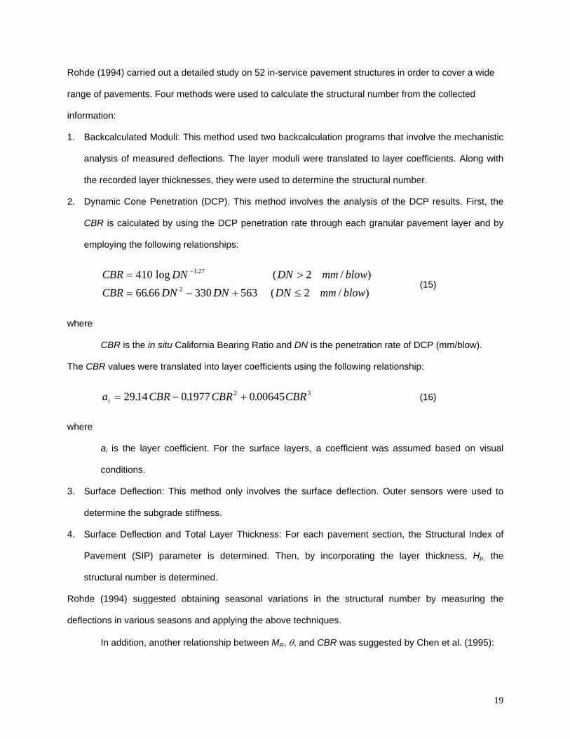
Rohde (1994) carried out a detailed study on 52 in-service pavement structures in order to cover a wide
range of pavements. Four methods were used to calculate the structural number from the collected
information:
1. Backcalculated Moduli: This method used two backcalculation programs that involve the mechanistic
analysis of measured deflections. The layer moduli were translated to layer coefficients. Along with
the recorded layer thicknesses, they were used to determine the structural number.
2. Dynamic Cone Penetration (DCP). This method involves the analysis of the DCP results. First, the
CBR is calculated by using the DCP penetration rate through each granular pavement layer and by
employing the following relationships:
CBR DN DN mm blowCBR DN DN DN mm blow
= >
= − + ≤
−410 266 66 330 563 2
1 27
2
log ( / ). ( / )
.
(15)
where
CBR is the in situ California Bearing Ratio and DN is the penetration rate of DCP (mm/blow).
The CBR values were translated into layer coefficients using the following relationship:
a CBR CBR CBRi = − +2914 01977 0 006452 3. . . (16)
where
a Bi B is the layer coefficient. For the surface layers, a coefficient was assumed based on visual
conditions.
3. Surface Deflection: This method only involves the surface deflection. Outer sensors were used to
determine the subgrade stiffness.
4. Surface Deflection and Total Layer Thickness: For each pavement section, the Structural Index of
Pavement (SIP) parameter is determined. Then, by incorporating the layer thickness, H Bp, B the
structural number is determined.
Rohde (1994) suggested obtaining seasonal variations in the structural number by measuring the
deflections in various seasons and applying the above techniques.
In addition, another relationship between MBR B, θ, and CBR was suggested by Chen et al. (1995):
20
( )M CBRR = ⋅ −490 243logθ (17)
Because the M BR B test result is stress-dependent, the coefficient that relates MBR B to CBR must be stress
dependent and not a unique or constant value.
Ping et al. (1996) conducted a study for the Florida Department of Transportation. This research
tried to correlate limerock bearing ratio (LBR, a Florida modification of the CBR) test results to the
AASHTO pavement design procedure. Twenty existing pavement sites were selected for the field plate
bearing load test (the LBR test). Laboratory samples were also prepared to cover the entire range of
desired moisture contents. In addition, selected laboratory compacted specimens were placed in a
soaking tank for approximately 2 days.
The LBR test results were compared with the optimum moisture content and the maximum dry
density values. The data were too scattered to infer suitable relationships between the optimum moisture
content and LBR values. However, the general trend for the density and LBR relationship is that the LBR
value augments as the density increases. This indicates that the LBR is more sensitive to density than to
the moisture content. The moisture content at the maximum dry density is generally the same as the
moisture content at the maximum LBR.
In general, the average moisture content obtained in the laboratory at the maximum LBR values
for all soils was not significantly different from the measured field moisture content. The maximum dry
densities compacted in the laboratory were also close to the average in situ-measured field densities.
However, the data were very scattered. Comparisons between the laboratory LBR results and the field
layer modulus were made and a general trend was observed. Although the data were scattered, there is
a slight increase in field layer modulus as LBR increases.
The LBR value was used as a correlation for soil support value (SSV) for the design of
pavements in Florida. Ping et al. (1996) identify two types of correlation :
SSV LBR andSSV LBR
( ) . log( ) .( ) . log( ) .1 4 596 05762 3325 0 672
= ⋅ −= ⋅ +
(18)
In addition, a correlation between the field resilient modulus and SSV is identified:
21
SSV ER( ) . log( ) .3 6 24 18 72= ⋅ − (19)
Correlations between the SSV results were also made. It is apparent that SSV(1) is higher than
SSV(2). The values for SSV(3), calculated from the field plate modulus, are much greater than those for
both SSV(1) and SSV(2). This means that the SSV obtained by correlating the field layer modulus is
greater than that obtained by correlating the laboratory LBR value. The difference between SSV(3) and
SSV(1) or SSV(2) may be due to the fact that LBR is a laboratory value that occurs at the optimum
moisture content and maximum density, whereas the field plate modulus (EBR B) is a field strength value that
is affected by many uncertain factors such as stress history of the pavement and the percentage of large
aggregates. SSV(1) predicts a modulus that is closer to the field modulus, SSV(3), than the existing
Florida design equation (SSV(2)); however, the field SSV(3) is generally higher than the laboratory
SSV(1). This is due to the major difference between the field and laboratory testing conditions.
2.2.1.4.4 Elastic Modulus of Base Layer
The use of the resilient modulus was extended by the 1986 AASHTO guide to be the predictor of
the base layer coefficient (a B2B). The following equation could be used to determine the layer coefficients for
a granular material from its elastic modulus (EBBSB):
( )a EBS2 100 249 0 977= ⋅ −. log . (20)
Richardson (1996) determined layer coefficients for cement-stabilized soil for use in the AASHTO
pavement design method. Two types of soils were examined: fine sand and silty clay. These were
blended with three different amounts of concrete sand. Three different cement contents were molded and
tested for static compressive chord modulus and unconfined compressive strength.
The methodology consisted in determining the moduli of the various materials and then
converting these moduli to layer coefficients. Layer coefficients were determined by using the modulus
values from the AASHTO pavement design guide nomograph. Regression equations based on strength,
dry unit weight, and cement content were developed to allow an for estimation of layer coefficients.
The best-fit equation for the data obtained is as follows:
E qc u= +91548 1314 9. . (21)
22
where
EBcB = chord modulus (MPa), and
q BuB = unconfined compressive strength.
A multiple regression model was fit to the obtained data. The best-fit model is as follows:
E Cc d= + +17759 579 77 9 6113. ( ) . ( )γ (22)
where
EBcB = chord modulus (MPa),
C = cement content (% by weight), and
γ BdB = dry unit weight (kg/m P
3P).
Layer coefficients were determined by use of the AASHTO nomograph. The equation for the
relationship between a B2B and the modulus was derived from the nomograph:
a Ec2 2 7170 0 49711= − +. . log (23)
where EBcB = elastic modulus (psi).
Substitution of the elastic moduli for the previous equation resulted in the layer coefficients. The layer
coefficient values ranged from 0.09 to 0.27, depending on the clay content, dry unit weight, and cement
content. Increasing the cement content and dry unit weight increased the layer coefficient, whereas
increasing the clay content lowered the layer coefficient.
A sensitivity analysis was performed by examining the effects of certain mixture variables
(cement and sand content) on the required thickness. It was found that all changes in cement content and
sand content are significant.
2.2.1.5 Wisconsin Department of Transportation
During the late 1980’s WisDOT began to rewrite the asphaltic specifications for mixture designs
to meet the demand for more durable asphaltic pavements that would accommodate the increased traffic
loading. During the 1990’s the reprocessing of asphaltic pavements into base course materials became
more prevalent.
Wisconsin’s flexible pavement design process, contained in the WisDOT Facilities Development
Manual (FDM), is based on the AASHTO design method. A structural number is used without the
drainage coefficients. The FDM refers to the layer coefficients as strength coefficients. These are listed in
Table 2, page 33. The FDM specifies that the strength coefficients are not absolute in the sense that they
represent a minimum strength value that can be expected throughout the state. Some of the materials,
such as Milled and Relayed Asphaltic Concrete, have a range of layer coefficients caused by variable
strength and stability. The FDM also provides a table titled “Relative Strength Coefficients for Granular
Subbase”, which supplies a strength coefficient based on % passing #40 sieve. The FDM states that
when recycled materials are used, the strength coefficients can be expected to be similar to those of
virgin materials.
The FDM limits to 10% the portion of strength a that granular sub-ase will contribute to the total
pavement structure. This takes place regardless of the strength coefficient or thickness involved. This will
ensure that the surface and base thicknesses used in the pavement structure are adequate and have a
built-in factor of safety.
In 1990, WisDOT published a report on layer coefficients for flexible pavements. The purpose of
the study, entitled “Layer Coefficients for Flexible Pavements,” was to evaluate new materials that are
used in flexible pavements. The goals were to establish AASHTO layer coefficients for use in the design,
establish a procedure that would allow for the determination of these coefficients, and provide input for
the new 1986 AASHTO design procedure. The study was to establish layer coefficients for new materials
being used and to evaluate the ones used at that time. The study also intended to develop a method of
determining layer coefficients for the new materials and provide inputs for the 1986 AASHTO Design
Guide. That study included both field and laboratory testing of typical asphalt mixes and base course
materials. It consisted in a comparison between the AASHTO empirical approach, as revised in the 1986
manual, and mechanistic analysis and design procedures.
Field-testing was conducted on several different pavements, including bases, subbases, recycled
asphalt concrete mixtures, and crack and seated overlays. The test sites varied in age from 1 to 9 years.
Field cores were taken as well as sample pits to determine laboratory determinations of layer coefficients.
Seasonal variations were investigated as well. Weaker pavement structures were found in spring, with
the subgrade as the culprit. The base materials were weaker in the fall, with this being exaggerated if a
subbase was present.
23
The study provided recommendations to use one layer coefficient for virgin asphalt mixes and
another for recycled mixes. The study did not address the specific type of mixes currently used by
WisDOT. Another important finding of that study was the need to relate layer coefficients to pavement
performance based on measuring load-induced material damage. The study also indicated that the
principle of the “weakest season” must be examined for individual materials. The researchers of the study
indicated that reliance on resilient modulus alone was tenuous at best. They suggested developing
rutting tests for asphalt layers and shear strength tests for granular materials to represent a parameter
that relates to performance. They found seasonal variations during the course of their testing and
suggested that these weakest seasons be taken into account. Finally, they recommended that a
mechanistic design approach be developed. They believed that this would provide a more in-depth
evaluation of material properties and their effects on pavement life.
Asphalt concrete layer coefficients were not changed and it was recommended that recycled
asphalt concrete be given the same layer coefficient as virgin material. Granular bases were given
values of 0.10, 0.14, and 0.16 for low, medium and high quality respectively. Open graded bases
received a layer coefficient of 0.12. A single value layer coefficient for crack and seated pavements were
not developed due to the randomness or the amount of cracks imparted on the concrete. It was
suggested in the study that the layer coefficient for cracked and seated pavement be reduced by 15 to
20% from the layer coefficients published at the time of the study.
2.2.2 Background to Field Measurements
The need for non-destructive methods to measure in situ material properties has resulted in
developing several methods. These methods can generally measure the total response of pavement
layers to loading or the transfer speed of loading waves in pavement layers. One of the most commonly
used methods is the Falling Weight Deflectometer (FWD).
2.2.2.1 The Falling Weight Deflectometer (FWD)
Applying a load to the pavement surface and measuring the resulting deflection can assess the
structural integrity of pavements. The FWD is one of the widely used deflection-based equipment in
pavement evaluation due to its ability to best simulate the dynamic moving wheel load at a wide range of
24
load levels. The FWD theory, field-testing procedures, analysis methods, and application in pavement
engineering are presented in this section.
The FWD equipment tests the pavement by dropping a weight from a specified height, which
corresponds to the load being simulated onto the pavement surface. Upon impact, several sensors
located at various radial distances from the loading center measure pavement deflections. The FWD test
is relatively quick, inexpensive, and closely simulates the deflection caused by a moving wheel load;
therefore, it has been widely used throughout the world in both academic research and industrial practice
(Houston et al. 1990).
Surface deflections constitute a bowl-shaped depression known as a deflection basin. The size,
depth, and shape of the deflection basin are a function of several variables, including the applied load,
the thickness, stiffness, and Poisson’s ratio, as well as other properties of the pavement structure
(Huang, 1993). Numerous backcalculation techniques have been developed to analyze deflection data
obtained from various types of pavement deflection equipment. Empirical correlations, such as deflection
parameters, which combine some or all of the measured deflections into a single value, are often used to
show the reciprocal relation between pavement properties. Horak (1987) provided a summary of
deflection parameters. Unfortunately, except for the subgrade layer, using these indices to predict the
properties of pavement structures is limited. Therefore, the use of deflections as a direct measure of the
pavement structural capacity should be avoided and a mechanistic analysis of the deflections is
recommended instead (FHWA, 1994).
Numerous studies have utilized FWD for the purpose of pavement evaluation and material
characterization. Two volumes of special technical reports from the American Society for Testing and
Materials (1989, 1994) are representative documents summarizing the development and application of
the FWD test. In this report, examples are presented from a previous research project, also sponsored by
WisDOT, that used FWD as one of the techniques to investigate the effect of freeze-thaw action on
pavement performance (Bosscher et al. 1997).
2.2.2.2 The Use of the Falling weight Deflectometer
Two procedures for determining layer coefficients from FWD deflections are documented in the
1986 AASHTO design guide. The first technique involves the backcalculation of layer moduli and relating
25
26
them to layer coefficients. This approach, which requires an exact knowledge of layer thickness, is time-
consuming and relies heavily on backcalculation expertise. The second approach uses outer deflection
sensors to determine subgrade stiffness and then applies the peak deflection, D B0B, to determine structural
number of he pavement. The problem with the second approach is that the subgrade is assumed to be an
infinitely thick linear-elastic material. Real pavements are not like that ; hence, only the first method will
be detailed.
The peak deflection measured below a FWD is a combination of the deflection in the subgrade
and the elastic compression of the pavement structure. Based on the fact that approximately 95 percent
of the deflections measured on the surface of a pavement originated below a line deviating 34 degrees
from the horizontal axis, it can be assumed that the surface deflection measured at an offset of 1.5 times
the pavement thickness originates entirely in the subgrade. By comparing this deflection to the peak
deflection, an index associated with the magnitude of deformation that occurs within the pavement
structure has been defined by Rohde (1994):
SIP D D Hp= −0 1 5. (24)
where
SIP = structural index of pavement,
D B0B = peak deflection,
D B1.5HpB = surface deflection, and
Hp = total pavement thickness.
Rohde (1994) hypothesized that the SIP is strongly correlated with the stiffness of the pavement
structure and subsequently with its structural number. To investigate this hypothesis and to develop a
relationship between FWD-measured surface deflections and the structural number of a pavement, a
large number of pavements were analyzed using the layered-elastic theory. A total of 7776 pavement
structures with a wide range of stiffness-thickness combinations were used. For each of the pavement
structures, the structural number was calculated using AASHTO guidelines:
SN h aEEi g
i
gi
n
=⎛
⎝⎜⎜
⎞
⎠⎟⎟
=∑
13
1 (25)
27
where
a BgB = layer coefficients of standard material,
EBgB = resilient modulus of standard material,
h Bi B = layer thickness (in), and
SN = structural number.
The best relationship was found after including the pavement thickness in the analysis. A
relationship with the following format was selected:
SN k SIP Hpk k= 12 3 (26)
where
SN = structural number,
SIP = structural index of pavement (µm),
Hp = total pavement thickness (mm), and
k B1B, k B2B, k B3B = coefficients.
The same rationale used to determine SN from surface deflections might be used to obtain the
sub-grade stiffness. Rohde (1994) has defined the Structural Index for the sub-grade (SIS) as:
SIS D DHp s= −1 5. (27)
where
SIS= structural index of the sub-grade
D BsB = surface deflection measured at an offset of (1.5Hp + 450 mm).
The SIS and the total pavement thickness were subsequently related to the sub-grade stiffness using the
following relationship:
E SIS Hpsgk k k= 10 4 5 6 (28)
where
EBsgB equals the sub-grade stiffness in MPa, and k B4B, k B5B, and k B6B are coefficients.
Sebaaly et al. (1989) investigated the relationship between surface cracking and the structural
capacity of both thin and thick pavement structures. The research examined the relationship between the

structural and functional performance parameters. Among the various performance parameters studied
were the surface cracking and the load-deflection response of the pavement structure under FWD
loading. By using cracking to indicate the structural condition, these systems assume the existence of a
relationship between surface cracking and the loss of structural capacity.
The results indicated that if pavement section showed an average rutting of 12.7 mm (0.5 in), the
failure mode was considered to be rutting; however, if the section showed a linear cracking value of
13670.6 mm/m2 (50 in/ft2), the failure mode was considered to be fatigue. The rate of crack propagation
through the asphalt depends on a combination of various factors:
1. the thickness of the asphalt layer,
2. the maximum size of the aggregate in the asphalt mix,
3. environmental conditions, and
4. the magnitude and frequency of loading.
Therefore, no general rate of crack propagation can be identified for any pavement system. When a
crack is initiated; the structural capacity of the pavement section is reduced. The crack decreases the
section of the asphalt layer available to resist tension, resulting in higher pavement deflections. In layer
theory analysis, it is assumed that the reduced structural capacity from fatigue cracking results from a
decrease in the modulus of the asphalt concrete layer.
2.2.3 Permanent Deformation Damage Functions
The research discussed in sections 2.2.1.3 and 2.2.1.4 indicates that various material properties,
measured through laboratory testing or field testing, have been correlated with layer coefficients.
However, this research has largely neglected to consider the failure behavior of materials. Several
studies, however, looked at the use of failure behavior using what are called damage functions.
Damage functions are defined as mathematical equations that can predict distresses or
reductions in performance measures as a fraction of a reference level of distress or reduction in
performance established as a failure condition. The failure condition can be represented as a structural
failure or a level of distress or loss of performance that may be expected to produce the need for major
repair or rehabilitation. The AASHO Road Test developed the following damage function for
serviceability:
28
29
β
ρ ⎟⎟⎠
⎞⎜⎜⎝
⎛=
Wg (29)
where
g = damage function, which ranges from 0 to 1 with increasing damage
W = number of 18-kip Equivalent Single Axle Loads (ESAL’s) applied
ρ = ESAL producing a damage level defined as failure
β= rate of damage increase
The values of ρ and β, which represent different types of distress and environmental zones, are functions
of a variety of independent variables. AASHO generally used a Present Serviceability Index (PSI) of 1.5
to represent total failure. This would be the terminal serviceability. A reduction of PSI to 1.5 caused by a
number of axle loads of an established magnitude is represented by a g equal to unity. Also, if a damage
function equals 0.5, this means that the PSI has been reduced by one-half the difference between the
initial PSI and the terminal PSI.
Cowher et al. (1975) summarized many previous studies on damage functions. A few of these
are described below. Cowher et al. (1975) also conducted an investigation into the cumulative damage of
asphalt materials.
Deacon (1965) studied the effects of compound loading on bituminous mixtures under laboratory
conditions. He developed a test that used a rectangular asphalt beam specimen. It had a two-point,
pneumatically-driven loading apparatus that produced a constant bending moment at the center of the
beam. With the simple and compound loading fatigue data used during the study, he developed the
following relationship to calculate the stiffness modulus:
∆
=**
IPKE (30)
where
E = deflection-based stiffness modulus
K = constant dependent on specimen geometry
P = total dynamic load applied upwards
30
I = moment of inertia of beam
∆ = dynamic center deflection
The stiffness decreased rapidly during the initial and the final phases of the test. During the intermediate
phases the stiffness was observed to gradually increase.
Deacon analyzed his data relying on Miner’s Hypothesis and its variations to derive the best
predictive relationship for a mean compound loading fracture life. Deacon found the best predictive model
by taking the experimental compound loading data and comparing it to the predicted results of nine
techniques. He compared the numbers generated in the following way:
DeviationMeasured Y
=Predicted (Y)- Measured (Y)
( ) (31)
where
Y = fracture life
The technique that had the least average squared deviation was considered the best technique.
It was concluded that a modification of Miner’s Hypothesis was the best predictive model. Deacon also
found that the order and magnitude of stress application was important. Finally, Deacon found that the
standard deviation of fracture life tends to increase as the stress level is decreased for simple loading
conditions.
For simple loading conditions, Deacon found the existence of a linear relationship between the
logarithm of the mean fatigue life and the logarithm of stress. Deacon also found that a larger load
duration would decrease the measured value of fracture life.
Cowher et al. (1975) also summarized a study done by McElvaney (1972) on the compound
loading behavior of bituminous mixtures. McElvaney studied the fatigue response of asphalt base course
specimens to compound loading in order to determine the predictive accuracy of Miner’s hypothesis.
Three types of constant loading tests were employed: sequence tests, repeated-block tests, and
temperature sequence tests. The tests consisted of a rotating cantilevered beam that was submersed in a
controlled temperature water bath. The specimen was rotated at 1000 RPM with a constant load applied
perpendicular to the axis of rotation. This produced a maximum bending stress at the necked down
portion of the specimen. Simple loading tests were also performed.
McElvaney found the existence of a linear relationship between the logarithm of applied stress
and the logarithmic mean number of cycles to failure. He also found that the fatigue life of a bituminous
material was sensitive to temperature changes; an increase in temperature caused a decrease in fatigue
life. Material variability on the cumulative cycles ratio was found to be significant at all stress levels.
Finally, McElvaney stated that a linear damage rule such as Miner’s Hypothesis is adequate for predicting
fatigue life under compound loading conditions.
Cowher et al. (1975) conducted their tests to determine the applicability of Miner’s hypothesis to
fatigue data obtained from dynamic indirect tensile tests. The indirect tensile test equipment used by
Cowher and his co-researchers is similar to the apparatus that will be used for this research project. Two
stress levels were used to evaluate the hypothesis.
Cowher et al. (1975) concluded that a log-log plot of stress as opposed to fatigue life for a given
set of environmental conditions is essentially linear. They also concluded that the aggregate type had no
effect on fatigue life for the entire range of stresses considered. For compound loading, they found that
the order and magnitude of the applied stresses have a significant effect on the fatigue life. It was also
concluded that Miner’s hypothesis is valid for the asphalt mixtures tested. Finally, they concluded that the
time deformation under compound loading conditions could be predicted from simple loading
considerations using a technique of linear summation of damage increments.
Cowher et al. (1975) recommended that future studies take into account the pseudo-random
loading spectra, which are more representative of actual field conditions. It was also recommended that
field conditions be incorporated into the laboratory testing so that a direct comparison can be made
between field and laboratory findings.
Rauhut et al. (1984) developed damage functions for both flexible and rigid pavements. The
damage functions developed were used to develop load equivalence factors for each of the significant
distresses investigated. They developed a computer program called DAMAGE that converted the
damage functions into load equivalence factors.
Rauhut et al. (1984) developed damage functions for rutting and serviceability loss using the
AASHO Road Test data. Their purpose was to investigate and validate the use of a combined
mechanistic and empirical modeling approach to develop damage functions. When Rauhut and his co-
31
32
researchers attempted to develop a damage function for fatigue cracking, they ran into problems with the
data. Most of the cracking failures occurred during the spring thaw, which resulted in clustered data. As a
result, it was not possible to develop meaningful regression analyses from that data.
They also modified ρ and β from the AASHO Road Test damage function (Eq. 29) to predict
rutting damage in the following way:
actSNLLL log*2291.1log*3852.1log*4786.1)log(*5221.25470.7log 221 ++++−=ρ
(32)
(33)
where
L B1 B= B Baxle load, kips
L B2B = axle code (1 for single axle, 2 for tandem)
SN = structural number
tBac B = asphalt concrete surface thickness, inches.
For serviceability loss the new ρ and β were:
ac
acac
tSNtLtLL
log*6412.1log*512.3]3539.0819.2[log]222.05658.3)[log(3647.8log 221
−+−++−++=ρ
(34)
acac
acacac
tSNt
tLttLL
log*4155.2log*0204.0]0265.0
2854.00728.0[log]0302.04017.03706.0)[log(7179.0log2
22
21
+−−
+++−++−=β
(35)
where the variables are similar to those in the rutting equations above.
For both the rut damage and serviceability loss Rauhut et al. (1984) found the existence of a good
correlation between their damage functions and the AASHO Road Test data.
log . . * log( ) . * log . * log . * logβ = − + + + +01432 0 7302 08890 0 0759 0 71801 2 2L L L SN tac
33
2.2.4 Rutting and Resilient Characteristics as Determined by Tri-Axial Testing
Unbound granular materials have a major function in the structural capacity of a highway
pavement. They provide a foundation that supports asphalt concrete layers and helps to support the
traffic that will use the constructed asphalt pavement. The unbound layers must exhibit high resilient
moduli and show low permanent deformation in order to reduce resilient deformation and rutting in the
asphalt pavement. The paragraphs that follow describe some studies that have been done in Europe on
the use of a tri-axial cell test to analyze the use of unbound granular materials as a structural layer in
pavements.
It is known that the characteristics of unbound granular materials are non-linear for both resilient
and permanent deformation. These characteristics include applied stress level (Hicks & Monismith,
1971), material type, density moisture content (Thom & Brown, 1987; 1988; 1989), and grading (Kamal &
Dawson, 1993). This literature review will concentrate on how the permanent deformation characteristics
or rutting features can be predicted by the use of the tri-axial test.
Dawson et al. (1993) conducted a study characterizing unbound granular materials as a function
of condition. They tested three aggregates in a pneumaticall-controlled 160-mm diameter, variable
confining pressure (VCP), tri-axial chamber. The purpose was to determine the effects of the moisture
content of the aggregate on the permanent and resilient deformations.
The samples were compacted using vibrocompression. This involves imparting an external
vibration onto a tube while subjecting the sample to a light static axial pressure. The sample diameter to
height ratio was held at 2 to 1 and air was used for the cell’s confining pressure.
Conditioning was achieved by cycling the confining pressure zero to 100 kPa and cycling the
deviator stress from 0 to 600 kPa. 20,000 conditioning cycles were applied. This resulted in a 2.0 gradient
between the p-q in an invariant stress space, where p is the mean normal stress and q is the deviator
stress. The permanent deformation tests were run by subjecting the specimens to 80,000 load repetitions
very similar to the ones used for conditioning.
To model plastic strain (εB1PB
p*P) they used an equation developed by Hornych et al. (1993).
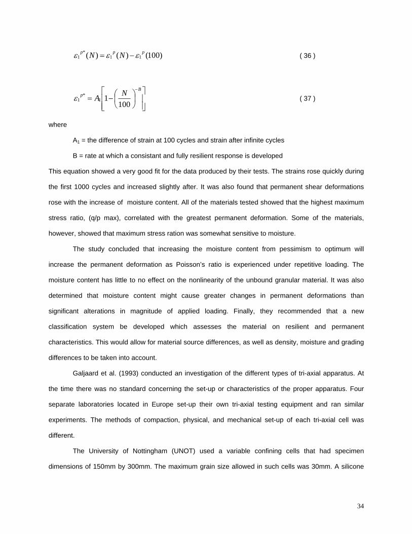
34
)100()()( 11*
1ppp NN εεε −= ( 36 )
⎥⎥⎦
⎤
⎢⎢⎣
⎡⎟⎠⎞
⎜⎝⎛−=
−Bp NA
10011
*1ε ( 37 )
where
AB1B = the difference of strain at 100 cycles and strain after infinite cycles
B = rate at which a consistant and fully resilient response is developed
This equation showed a very good fit for the data produced by their tests. The strains rose quickly during
the first 1000 cycles and increased slightly after. It was also found that permanent shear deformations
rose with the increase of moisture content. All of the materials tested showed that the highest maximum
stress ratio, (q/p max), correlated with the greatest permanent deformation. Some of the materials,
however, showed that maximum stress ration was somewhat sensitive to moisture.
The study concluded that increasing the moisture content from pessimism to optimum will
increase the permanent deformation as Poisson’s ratio is experienced under repetitive loading. The
moisture content has little to no effect on the nonlinearity of the unbound granular material. It was also
determined that moisture content might cause greater changes in permanent deformations than
significant alterations in magnitude of applied loading. Finally, they recommended that a new
classification system be developed which assesses the material on resilient and permanent
characteristics. This would allow for material source differences, as well as density, moisture and grading
differences to be taken into account.
Galjaard et al. (1993) conducted an investigation of the different types of tri-axial apparatus. At
the time there was no standard concerning the set-up or characteristics of the proper apparatus. Four
separate laboratories located in Europe set-up their own tri-axial testing equipment and ran similar
experiments. The methods of compaction, physical, and mechanical set-up of each tri-axial cell was
different.
The University of Nottingham (UNOT) used a variable confining cells that had specimen
dimensions of 150mm by 300mm. The maximum grain size allowed in such cells was 30mm. A silicone
35
oil was used as the cell fluid. The load cell and the axial LVDTs were located inside the cell as well as
radial deformation rings. There was also an additional pressure sensor located inside the cell to measure
cell pressure.
The compaction was done in an alluminum split ring mold. Four layeres were compacted using
an external vibration on the split ring while a small surcharge load was applied axially. When completed,
the split ring was removed. Then, a vacuum was applied to the inside of the specimen ; a second
membrain was placed on the specimen, and it was moved to the cell base.
The Laboratorio Nacional de Engenharial Civil (LNEC) used a 300mm by 600mm vacuum
constant confining pressure rig. The system has no tri-axial cell ; confining pressure was simulated by
applying a vacuum to the inside of the specimen. The compaction was completed by using a split ring
mold. A ten-layer compaction was implemented with the use of a vibrating hammer.
Le Laboratoire Central des Ponts et Chaussees (LCRF) employed a pneumatically powered 160
mm by 320 mm variable confining pressure rig. The maximum grain size allowed in this set-up was 31.5
mm. They positioned their load cell inside the pressure cell and used axial LVDTs, also located inside the
tri-axial cell. Three radial LVDTs, placed 120° apart, were used instead of a radial ring device that was
employed by the previous two laboratories mentioned. The confining pressure was developed by air
pressure.
A vibrocompression technique was used to complete the compaction of the specimens. This
consisted of a PVC container that experienced a horizontal vibration and a system to apply a small
vertical load during the vibrating. The compaction using this method was completed in one layer at
optimum moisture content. To achieve the proper water content, the specimens would be dried at 40° C
until the desired moisture content was met.
Delft University of Technology (DUT) had an apparatus that was a 400mm by 800mm vacuum
constant confining pressure rig. Like the LNEC the confining pressure was induced by applying a vacuum
to the inside of the specimen. Again, there was no tri-axial cell needed to complete the test. Like all the
others, they used axial transducers placed at the 1/3 and 2/3 points of the specimen to avoid edge
effects. To measure radial deformations, proximity transducers located on the rings that hold the axial
transducers were used.
36
Manual compaction took place in eight layers using a heavy tamper. After every second layer,
further compaction was completed by using a compaction plate at the end of an actuator, a static load of
10kN for 30 minutes, plus a cyclic half-sine load with a frequency of 7Hz and an amplitude of 40kN.
Each laboratory completed three identical tests using a q/p stress ratio of 3. The specimens
experienced 20,000 cycles of conditioning. The conditions were 50kPa confining pressure (σ B3B), a
minimum deviator stress of 0kPa (qBminB), and a cyclic deviator stress set at 130kPa (q Br B). Before and after
the coditioning, the specimens received five cycles of isotropic loading. For these loadings, the initial cell
pressure was zero and cyclic cell pressure was 50kPa. The testing portion of the tests was done in a
series of 12 cyclic loadings of 100 cycles each. The parameters are as follows:
σ B3B = 15kPa, q BminB = 0, q Br B = 15; 30; 45; 60kPa (38)
σ B3B = 30kPa, q BminB = 0, q Br B = 25; 50; 75; 100kPa (39)
σ B3B = 45kPa, q BminB = 0, q Br B = 30; 60; 90; 120kPa. (40)
Finally, an additional isotropic loading identical to the previous ones was applied.
The permanent strains used for the analysis were obtained during the conditioning of the
specimens. The axial permanent strains (εB1PB
pP) turned out to be quite different from all the laboratories. It
was concluded that the differences could be attributed to the differences in the compaction methods
used.
The study developed recommendations for tri-axial testing unbound materials. The first thing
mentioned was the necessity of using a reliable compaction method. The vibrocompression method used
at the LRSB was recommended. The method was quick and provided specimens with a homogenous
density profile. They also qualified the results coming from this method of compaction as being good.
A testing system that has a resolution of 10 P
-5P in strains should be used due to the nature of the
very small resilient strains. The larger the specimen, the more reliable the results. The 300mm by 600mm
size was pointed out because of the larger size and the ability to still perform a variable confining
pressure test (VCP). The VCP was found to yield more reliable results.
LRSB conducted a separate analysis on compaction profiles produced from both a
vibrocompression method and a vibrating hammer method compacted in 3, 5, and 7 layers. The densities
varied from 70kg/mP
3P (vibrocompression and 7-layer vibration hammer) to 300kg/mP
3P (3-layer vibration
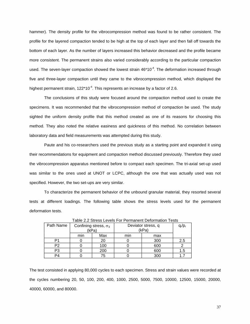
37
hammer). The density profile for the vibrocompression method was found to be rather consistent. The
profile for the layered compaction tended to be high at the top of each layer and then fall off towards the
bottom of each layer. As the number of layers increased this behavior decreased and the profile became
more consistent. The permanent strains also varied considerably according to the particular compaction
used. The seven-layer compaction showed the lowest strain 46*10 P
-4P. The deformation increased through
five and three-layer compaction until they came to the vibrocompression method, which displayed the
highest permanent strain, 122*10 P
-4P. This represents an increase by a factor of 2.6.
The conclusions of this study were focused around the compaction method used to create the
specimens. It was recommended that the vibrocompression method of compaction be used. The study
sighted the uniform density profile that this method created as one of its reasons for choosing this
method. They also noted the relative easiness and quickness of this method. No correlation between
laboratory data and field measurements was attempted during this study.
Paute and his co-researchers used the previous study as a starting point and expanded it using
their recommendations for equipment and compaction method discussed previously. Therefore they used
the vibrocompression apparatus mentioned before to compact each specimen. The tri-axial set-up used
was similar to the ones used at UNOT or LCPC, although the one that was actually used was not
specified. However, the two set-ups are very similar.
To characterize the permanent behavior of the unbound granular material, they resorted several
tests at different loadings. The following table shows the stress levels used for the permanent
deformation tests.
Table 2.2 Stress Levels For Permanent Deformation Tests Path Name Confining stress, σ B3B
(kPa) Deviator stress, q
(kPa) q Br B/p Br B
min Max min max P1 0 20 0 300 2.5 P2 0 100 0 600 2 P3 0 200 0 600 1.5 P4 0 75 0 300 1.7
The test consisted in applying 80,000 cycles to each specimen. Stress and strain values were recorded at
the cycles numbering 20, 50, 100, 200, 400, 1000, 2500, 5000, 7500, 10000, 12500, 15000, 20000,
40000, 60000, and 80000.

38
The modeling of the permanent behavior consisted of two aspects: the variations between the
number of cycles and the permanent strains and any relations between the stresses and the permanent
strains. The model used here was the one developed by Hornych et al. (1993), the same model that was
used in the research by Dawson et al. (1993).
)100()()( 11*
1ppp NN εεε −= (41)
⎥⎥⎦
⎤
⎢⎢⎣
⎡⎟⎠⎞
⎜⎝⎛−=
−Bp NA
10011
*1ε (42)
where
AB1B = the difference of strain at 100 cycles and strain after infinite cycles
B = rate at which a consistant and fully resilient response is developed
The model deals with the axial permanent strain occurring at 100 cycles. To create the power law
relation, the first equation was integrated after it had been noticed that unbound granular materials have a
linear relation between the ln (δεB1PB
pP/δN) versus ln (N).
)ln(*)/ln( 1 NbaNp +=δδε (43)
The integration led to:
cNbe b
ap +
+= +1
1 *1
ε (44)
where
c = a constant.
The expression then becomes the power law shown above with two parameters AB1B and B. AB1B represents
the limit of the permanent strain for a given cyclic loading.
A relation between the AB1B parameter and the axial permanent strain was found. This represents
the influence of the stress level on the specimen.
⎟⎟⎠
⎞⎜⎜⎝
⎛+
−
⎟⎟⎠
⎞⎜⎜⎝
⎛+
=
*
*
1
ppqba
ppq
A ( 45 )
where

a, b = positive parameters
p* = the parameter related to the failure line of the material (see figure below)
S
p*
Failure line qf = M*p + S
q
p
Figure 2.1 Determination of the stress p*
This hyperbolic relationship is similar to the one proposed by Lentz and Balady (1980). A1
depends only on the ratio q/(p+p*). When A1 increases, the stress ratio increases as well. The equation
for A1 also shows that there is a maximum limit for q/(p+p*) ; this represents the failure of the material: q/
(p+p*) max = a/b = M, the slope of the failure lin. It was also observed that p* = S/M.
Puate and his co-researchers explained that these properties of the A1 and failure line
relationships present a simple method to accurately describe the plastic behavior of unbound granular
materials. It was also noted that the parameters a, b, M, and S can be obtained by successive
approximations to the value of p*. When the correlation ratio is at its highest the representative value can
be obtained.
39
CHAPTER THREE
MATERIAL COLLECTION, SPECIMEN PREPARATION, DATA COLLECTION, AND
CALCULATION
This chapter is divided into three sections: material and project descriptions, collection and
analysis of the field data, and laboratory data collection and analysis. To collect a wide range of
materials, the Wisconsin Department of Transportation (WISDOT) specified a list of projects to choose
from and specified a group of materials to potentially analyze.
The particular projects to focus on were selected by the research group at the University of
Wisconsin, Madison, based primarily on when the individual projects were being constructed. After
collecting the materials and the field data, the members of the Technical Oversight Committee (TOC) for
the project, organized by the WISDOT, narrowed down the list of materials to those they felt were the
most important for immediate analysis and implementation of results.
3.1 Material and Project Descriptions
Two general types of materials were selected for this project: hot mix asphalt (HMA) and recycled
granular base course. Four types of HMA and three types of base course materials were collected from
various projects throughout the state. Table 3.1 on page 43 summarizes the materials used in this
research.
3.1.1 Bound Materials
Four types of bound materials were selected: Superpave (SHRP), Stone Matrix Asphalt (SMA),
High Volume (HV) mix, Medium Volume (MV) mix and Asphalt Base Course (ABC). These asphalt
mixtures vary mainly in their gradations; however, the asphalt binder type and optimum content also vary.
40
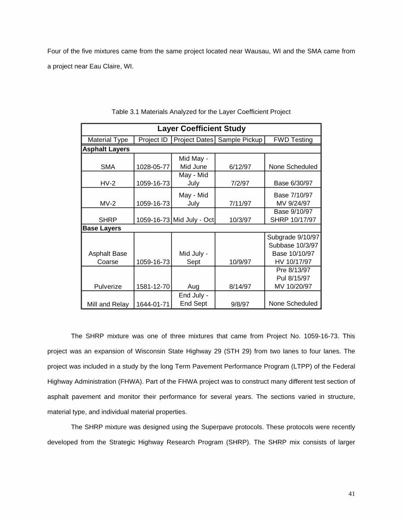
Four of the five mixtures came from the same project located near Wausau, WI and the SMA came from
a project near Eau Claire, WI.
Table 3.1 Materials Analyzed for the Layer Coefficient Project
Material Type Project ID Project Dates Sample Pickup FWD TestingAsphalt Layers
SMA 1028-05-77Mid May - Mid June 6/12/97 None Scheduled
HV-2 1059-16-73May - Mid
July 7/2/97 Base 6/30/97
MV-2 1059-16-73May - Mid
July 7/11/97Base 7/10/97 MV 9/24/97
SHRP 1059-16-73 Mid July - Oct 10/3/97Base 9/10/97
SHRP 10/17/97Base Layers
Asphalt Base Coarse 1059-16-73
Mid July - Sept 10/9/97
Subgrade 9/10/97 Subbase 10/3/97 Base 10/10/97 HV 10/17/97
Pulverize 1581-12-70 Aug 8/14/97
Pre 8/13/97 Pul 8/15/97
MV 10/20/97
Mill and Relay 1644-01-71End July - End Sept 9/8/97 None Scheduled
Layer Coefficient Study
The SHRP mixture was one of three mixtures that came from Project No. 1059-16-73. This
project was an expansion of Wisconsin State Highway 29 (STH 29) from two lanes to four lanes. The
project was included in a study by the long Term Pavement Performance Program (LTPP) of the Federal
Highway Administration (FHWA). Part of the FHWA project was to construct many different test section of
asphalt pavement and monitor their performance for several years. The sections varied in structure,
material type, and individual material properties.
The SHRP mixture was designed using the Superpave protocols. These protocols were recently
developed from the Strategic Highway Research Program (SHRP). The SHRP mix consists of larger
41

sized aggregates with minimum amounts of natural sands. The binder used for this mix was a PG58-22.
The material properties for the SHRP mix, as reported by the HMA producer, are shown in Table 3.2.
42
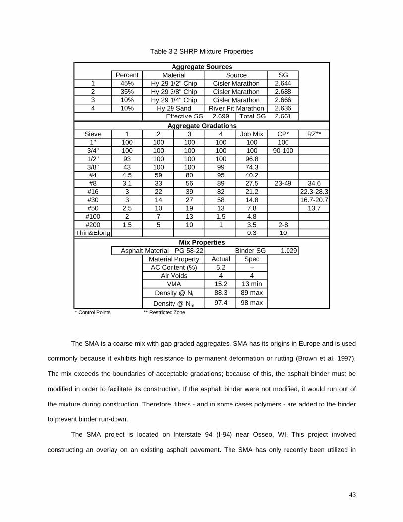
Table 3.2 SHRP Mixture Properties
Percent SG1 45% 2.6442 35% 2.6883 10% 2.6664 10% 2.636
Effective SG 2.699 Total SG 2.661
Sieve 1 2 3 4 Job Mix CP* RZ*1" 100 100 100 100 100 100
3/4" 100 100 100 100 100 90-1001/2" 93 100 100 100 96.83/8" 43 100 100 99 74.3#4 4.5 59 80 95 40.2#8 3.1 33 56 89 27.5 23-49 34.6#16 3 22 39 82 21.2 22.3-28.3#30 3 14 27 58 14.8 16.7-20.7#50 2.5 10 19 13 7.8 13.7
#100 2 7 13 1.5 4.8#200 1.5 5 10 1 3.5 2-8
Thin&Elong 0.3 10
Asphalt Material PG 58-22 Binder SG 1.029Actual Spec
5.2 --4 4
15.2 13 min88.3 89 max97.4 98 max
* Control Points ** Restricted Zone
*
Aggregate SourcesMaterial Source
Hy 29 1/2" Chip Cisler MarathonHy 29 3/8" Chip Cisler MarathonHy 29 1/4" Chip Cisler Marathon
Hy 29 Sand River Pit Marathon
Aggregate Gradations
Mix Properties
Density @ Ni
Density @ Nm
Material PropertyAC Content (%)
Air VoidsVMA
The SMA is a coarse mix with gap-graded aggregates. SMA has its origins in Europe and is used
commonly because it exhibits high resistance to permanent deformation or rutting (Brown et al. 1997).
The mix exceeds the boundaries of acceptable gradations; because of this, the asphalt binder must be
modified in order to facilitate its construction. If the asphalt binder were not modified, it would run out of
the mixture during construction. Therefore, fibers - and in some cases polymers - are added to the binder
to prevent binder run-down.
The SMA project is located on Interstate 94 (I-94) near Osseo, WI. This project involved
constructing an overlay on an existing asphalt pavement. The SMA has only recently been utilized in
43
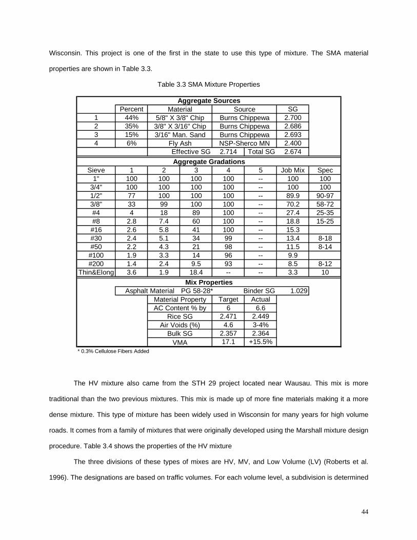
Wisconsin. This project is one of the first in the state to use this type of mixture. The SMA material
properties are shown in Table 3.3.
Table 3.3 SMA Mixture Properties
Percent SG1 44% 2.7002 35% 2.6863 15% 2.6934 6% 2.400
Effective SG 2.714 Total SG 2.674
Sieve 1 2 3 4 5 Job Mix Spe1" 100 100 100 100 -- 100 100
3/4" 100 100 100 100 -- 100 1001/2" 77 100 100 100 -- 89.9 90-973/8" 33 99 100 100 -- 70.2 58-72#4 4 18 89 100 -- 27.4 25-35#8 2.8 7.4 60 100 -- 18.8 15-25#16 2.6 5.8 41 100 -- 15.3#30 2.4 5.1 34 99 -- 13.4 8-18#50 2.2 4.3 21 98 -- 11.5 8-14
#100 1.9 3.3 14 96 -- 9.9#200 1.4 2.4 9.5 93 -- 8.5 8-12
Thin&Elong 3.6 1.9 18.4 -- -- 3.3 10
Asphalt Material PG 58-28* Binder SG 1.029Target Actual
6 6.62.471 2.4494.6 3-4%
2.357 2.36417.1 +15.5%
* 0.3% Cellulose Fibers Added
Bulk SGVM
c
A
Material PropertyAC Content % by
Rice SGAir Voids (%)
Fly Ash NSP-Sherco MN
Aggregate Gradations
Mix Properties
3/8" X 3/16" Chip Burns Chippewa3/16" Man. Sand Burns Chippewa
Aggregate SourcesMaterial Source
5/8" X 3/8" Chip Burns Chippewa
The HV mixture also came from the STH 29 project located near Wausau. This mix is more
traditional than the two previous mixtures. This mix is made up of more fine materials making it a more
dense mixture. This type of mixture has been widely used in Wisconsin for many years for high volume
roads. It comes from a family of mixtures that were originally developed using the Marshall mixture design
procedure. Table 3.4 shows the properties of the HV mixture
The three divisions of these types of mixes are HV, MV, and Low Volume (LV) (Roberts et al.
1996). The designations are based on traffic volumes. For each volume level, a subdivision is determined
44

by the mixtures gradation. A number represents the gradations: lower numbers represent courser
mixtures and higher numbers signify finer gradations. The numbers range from one to five. The courser
gradations are used for binder course layers and the finer gradations are used for surface course layers.
The HV and MV collected for this project were both of gradation type 2.
The MV mixture was used for the construction of temporary traffic crossovers. The main
difference between this mixture and the HV is that the MV has less manufactured sand. Therefore its
percentage of screenings and natural sand is higher. Out of all the surface mixes it has the finest
gradation and the greatest percentage of natural sands. The MV mixture properties are shown in Table
3.5.
The ABC material was also collected from the STH 29 project near Wausau. Since these mixes
are designed as base courses, they tend to be gap-graded with a relatively large amount of natural sand.
The conventional wisdom is that mixes with large amounts of natural sand are weak mixtures. Since the
stresses at the base level will be lower than those at the surface level, the quality and strength of the mix
need not equal those of a surface mixture. The addition of the asphalt is believed to strengthen the
mixture to a level above that of an open-graded base course. The ABC mixture properties are shown in
Table 3.6.
All of these mixes were designed and constructed by the Mathy Construction Co. The data for the
material’s property tables was taken directly from their reports on each asphalt mixture design.
45
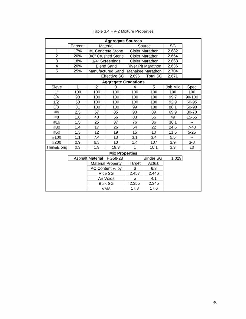
Table 3.4 HV-2 Mixture Properties
Percent SG1 17% 2.6822 20% 2.6643 18% 2.6634 20% 2.6365 25% 2.704
Effective SG 2.696 Total SG 2.671
Sieve 1 2 3 4 5 Job Mix Spe1" 100 100 100 100 100 100 100
3/4" 98 100 100 100 100 99.7 90-1001/2" 58 100 100 100 100 92.9 60-953/8" 31 100 100 99 100 88.1 50-90#4 2.3 67 85 93 89 69.9 30-70#8 1.6 40 56 83 56 49 15-55#16 1.5 25 37 76 36 36.1 --#30 1.4 17 26 54 22 24.6 7-40#50 1.3 12 19 15 10 11.5 5-25
#100 1.1 7.4 13 3.1 3.4 5.5 --#200 0.9 6.3 10 1.4 107 3.9 3-8
Thin&Elong 0.3 1.9 19.3 1 10.1 3.3 10
Asphalt Material PG58-28 Binder SG 1.029Target Actual
6 6.32.457 2.446
5 4.12.355 2.34517.8 17.6
c
Aggregate SourcesMaterial Source
#1 Concrete Stone Cisler Marathon3/8" Crushed Stone Cisler Marathon
1/4" Screenings Cisler MarathonBlend Sand River Pit Marathon
Manufactured Sand Manakee Marathon
Aggregate Gradations
Mix Properties
AC Content % by Rice SGAir VoidsBulk SG
VMA
Material Property
46
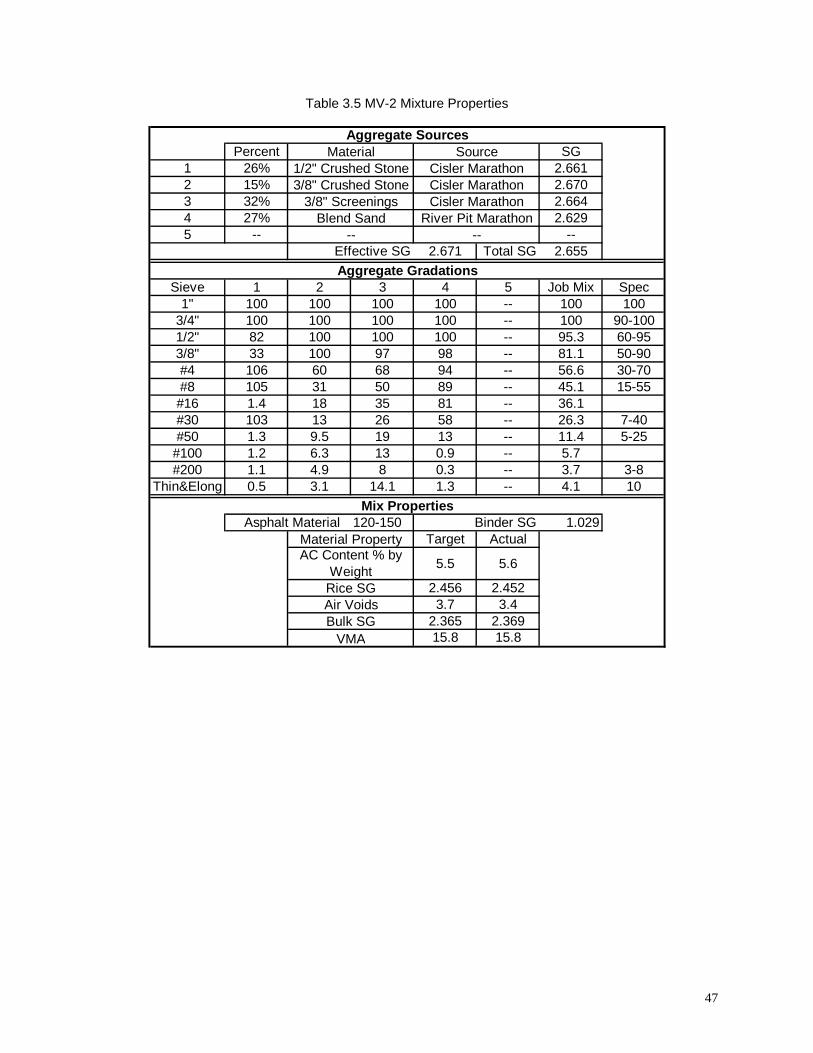
Table 3.5 MV-2 Mixture Properties
Percent SG1 26% 2.6612 15% 2.6703 32% 2.6644 27% 2.6295 -- --
Effective SG 2.671 Total SG 2.655
Sieve 1 2 3 4 5 Job Mix Spe1" 100 100 100 100 -- 100 100
3/4" 100 100 100 100 -- 100 90-1001/2" 82 100 100 100 -- 95.3 60-953/8" 33 100 97 98 -- 81.1 50-90#4 106 60 68 94 -- 56.6 30-70#8 105 31 50 89 -- 45.1 15-55#16 1.4 18 35 81 -- 36.1#30 103 13 26 58 -- 26.3 7-40#50 1.3 9.5 19 13 -- 11.4 5-25
#100 1.2 6.3 13 0.9 -- 5.7#200 1.1 4.9 8 0.3 -- 3.7 3-8
Thin&Elong 0.5 3.1 14.1 1.3 -- 4.1 10
Asphalt Material 120-150 Binder SG 1.029Target Actual
5.5 5.6
2.456 2.4523.7 3.4
2.365 2.36915.8 15.8
c
Aggregate SourcesMaterial Source
1/2" Crushed Stone Cisler Marathon3/8" Crushed Stone Cisler Marathon
3/8" Screenings Cisler MarathonBlend Sand River Pit Marathon
-- --
Aggregate Gradations
Mix Properties
Material PropertyAC Content % by
WeightRice SGAir VoidsBulk SG
VMA
47
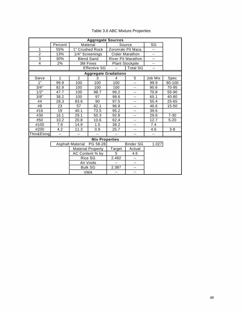
Table 3.6 ABC Mixture Properties
Percent SG1 55% --2 13% --3 30% --4 2% --
Effective SG -- Total SG --
Sieve 1 2 3 4 5 Job Mix Spec1" 99.9 100 100 100 -- 99.9 90-100
3/4" 82.9 100 100 100 -- 90.6 70-951/2" 47.7 100 98.7 99.2 -- 70.8 55-903/8" 38.2 100 97 98.6 -- 65.1 40-80#4 28.3 83.6 90 97.5 -- 55.4 25-65#8 23 57 82.1 96.8 -- 46.6 15-50
#16 19 40.1 73.5 95.2 -- 39.6#30 16.1 29.1 50.3 92.8 -- 29.6 7-30#50 10.2 20.8 10.6 62.4 -- 12.7 5-20
#100 7.8 14.9 1.5 38.2 -- 7.4#200 4.2 11.3 0.9 25.7 -- 4.6 3-8
Thin&Elong -- -- -- -- -- --
Asphalt Material PG 58-28 Binder SG 1.027Target Actual
5 4.62.492 --
-- --2.387 --
-- --Bulk SG
VMA
Material PropertyAC Content % by
Rice SGAir Voids
3M Fines Plant Stockpile
Aggregate Gradations
Mix Properties
1/4" Screenings Cisler MarathonBlend Sand River Pit Marathon
Aggregate SourcesMaterial Source
1" Crushed Rock Zoromski Pit Mara.
48
3.1.2 Unbound Materials
Using recycled surface course materials for base layers is becoming popular given today’s
concerns with environmental protection. Recycling materials eliminates them from landfills by actually
putting them to good use after their life as a surface course has come to an end.
There are two primary methods of recycling asphalt surface layers. One is called pulverizing and
the other milling. They basically involve the same process: the pavement is ground using large metal
teeth on a rotating drum until no pieces generally larger than one inch are left. The difference between
the two methods is in the machinery. The pulverizing equipment grinds up the material and then drops it
in the same location from where it was taken. On the other hand, the milling equipment lifts up the
recycled pavement and puts it on a conveyor. The conveyor leads to the end of the machine where the
recycled material can either be put into a truck or dropped to the ground. Project design and equipment
availability determine which process will be used, but the two are essentially the same.
Many times virgin or shoulder aggregates are added to the recycled material. Some projects will
recycle the entire surface layer, whereas at other times only a partial milling will be performed. Once
these materials are broken down they are compacted and used as base layers for a new asphalt
pavement that will be paved over the top. They are generally compacted to 95% of their maximum
density. Other processes are then introduced to add asphalt at low contents or emulsion to help bind the
recycled material.
The materials used for this project consisted of a pulverized asphalt pavement and a milled
asphalt pavement. The pulverized material had a 13% shoulder aggregate added in during the
pulverization process. The pulverizer ground up the entire surface layer and part of the granular shoulder.
The milled material had no outside aggregates added during the recycling process. However, it was
decided by the WDOT to add a 50% #2 of open-graded virgin aggregate for the laboratory testing.
The virgin aggregate for the milled asphalt was collected from the Payne and Dolan facility
located in Verona, WI. The two materials were mixed by weight in the laboratory at equal proportions
making a 50-50 blend.
The milled material was gathered from a project on US Highway 14 (USH 14) just south
of La Crosse, WI. The project was a full-depth mill. The material was dropped onto the existing base
49
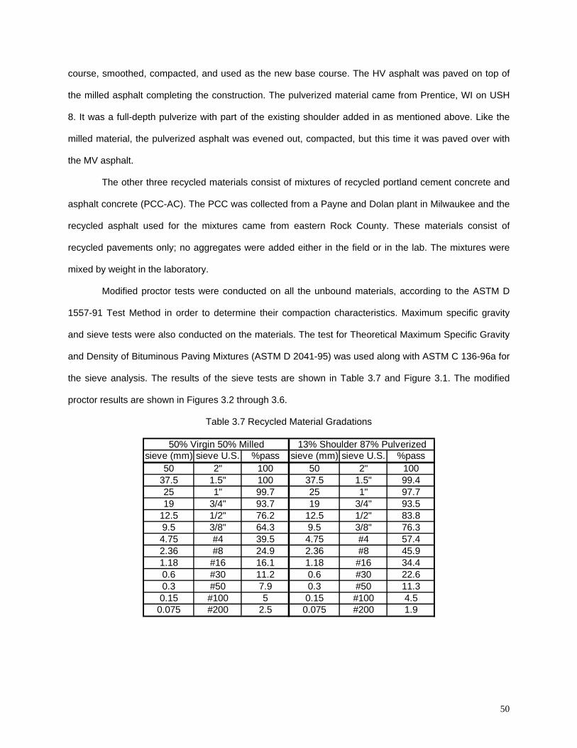
course, smoothed, compacted, and used as the new base course. The HV asphalt was paved on top of
the milled asphalt completing the construction. The pulverized material came from Prentice, WI on USH
8. It was a full-depth pulverize with part of the existing shoulder added in as mentioned above. Like the
milled material, the pulverized asphalt was evened out, compacted, but this time it was paved over with
the MV asphalt.
The other three recycled materials consist of mixtures of recycled portland cement concrete and
asphalt concrete (PCC-AC). The PCC was collected from a Payne and Dolan plant in Milwaukee and the
recycled asphalt used for the mixtures came from eastern Rock County. These materials consist of
recycled pavements only; no aggregates were added either in the field or in the lab. The mixtures were
mixed by weight in the laboratory.
Modified proctor tests were conducted on all the unbound materials, according to the ASTM D
1557-91 Test Method in order to determine their compaction characteristics. Maximum specific gravity
and sieve tests were also conducted on the materials. The test for Theoretical Maximum Specific Gravity
and Density of Bituminous Paving Mixtures (ASTM D 2041-95) was used along with ASTM C 136-96a for
the sieve analysis. The results of the sieve tests are shown in Table 3.7 and Figure 3.1. The modified
proctor results are shown in Figures 3.2 through 3.6.
Table 3.7 Recycled Material Gradations
sieve (mm) sieve U.S. %pass sieve (mm) sieve U.S. %pass50 2" 100 50 2" 100
37.5 1.5" 100 37.5 1.5" 99.425 1" 99.7 25 1" 97.719 3/4" 93.7 19 3/4" 93.5
12.5 1/2" 76.2 12.5 1/2" 83.89.5 3/8" 64.3 9.5 3/8" 76.34.75 #4 39.5 4.75 #4 57.42.36 #8 24.9 2.36 #8 45.91.18 #16 16.1 1.18 #16 34.40.6 #30 11.2 0.6 #30 22.60.3 #50 7.9 0.3 #50 11.30.15 #100 5 0.15 #100 4.5
0.075 #200 2.5 0.075 #200 1.9
50% Virgin 50% Milled 13% Shoulder 87% Pulverized
50
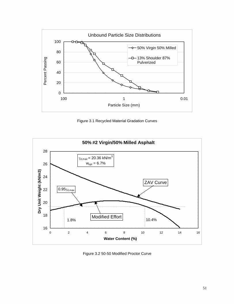
51
Unbound Particle Size Distributions
0
20
40
60
80
100
0.011100
Particle Size (mm)
Per
cent
Pas
sing
50% Virgin 50% Milled
13% Shoulder 87%Pulverized
Figure 3.1 Recycled Material Gradation Curves
50% #2 Virgin/50% Milled Asphalt
16
18
20
22
24
26
28
0 2 4 6 8 10 12 14 16
Water Content (%)
Dry
Uni
t Wei
ght (
kN/m
3)
γd,max = 20.36 kN/m3
wopt = 6.7%
1.8% 10.4%
0.95γd,max
ZAV Curve
Modified Effort
Figure 3.2 50-50 Modified Proctor Curve
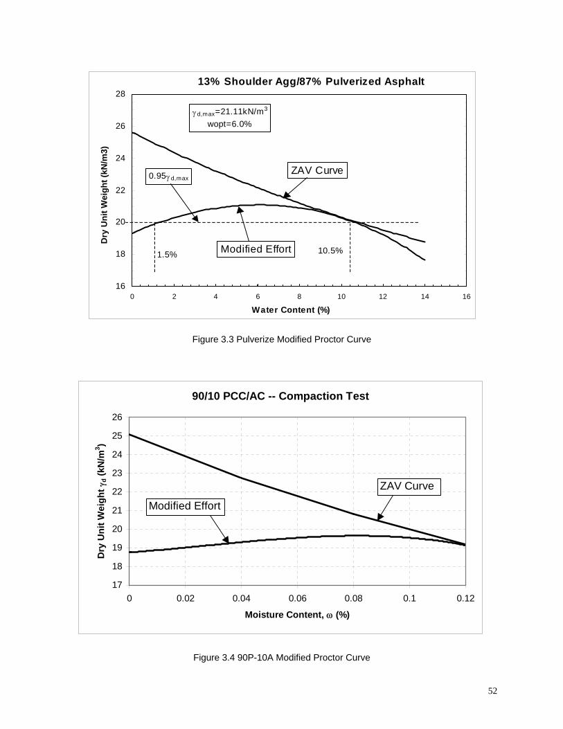
52
13% Shoulder Agg/87% Pulverized Asphalt
16
18
20
22
24
26
28
0 2 4 6 8 10 12 14 16
Water Content (%)
Dry
Uni
t Wei
ght (
kN/m
3)
1.5% 10.5%
0.95γ d,max
γ d,max=21.11kN/m3
wopt=6.0%
Modified Effort
ZAV Curve
Figure 3.3 Pulverize Modified Proctor Curve
90/10 PCC/AC -- Compaction Test
17
18
19
20
21
22
23
24
25
26
0 0.02 0.04 0.06 0.08 0.1 0.12
Moisture Content, ω (%)
Dry
Uni
t Wei
ght γ
d (kN
/m3 )
ZAV Curve
Modified Effort
Figure 3.4 90P-10A Modified Proctor Curve
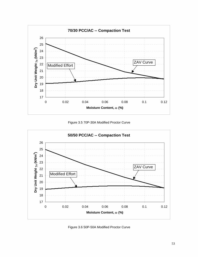
53
70/30 PCC/AC -- Compaction Test
17
18
19
20
21
22
23
24
25
26
0 0.02 0.04 0.06 0.08 0.1 0.12
Moisture Content, ω (%)
Dry
Uni
t Wei
ght γ
d (kN
/m3 )
ZAV CurveModified Effort
Figure 3.5 70P-30A Modified Proctor Curve
50/50 PCC/AC -- Compaction Test
17
18
19
20
21
22
23
24
25
26
0 0.02 0.04 0.06 0.08 0.1 0.12
Moisture Content, ω (%)
Dry
Uni
t Wei
ght γ
d (kN
/m3 )
ZAV Curve
Modified Effort
Figure 3.6 50P-50A Modified Proctor Curve

3.2 Field Data Collection and Analysis
3.2.1 Field Data Collection
The FWD was used to collect all of the field data for this research. The mechanism and the
methods behind it were explained in Chapter 2. It was not feasible to test all of the asphalt sections
considered as part of the original work plan. Also, some sections could not be tested due to the manner in
which they were constructed. The reason for fieldwork in this research project was to be able to verify the
laboratory numbers with actual field data.
Pavement sections that will be covered in this section include the MV, ABC, and the SHRP
sections. Field and laboratory tests were conducted on all the materials just listed. The remaining
materials did not undergo FWD testing.
The spacing of the FWD testing locations was determined from project to project depending on
the geometry of the individual projects. An attempt was made to cover the entire length of the project. All
of the projects varied in length; therefore, the spacing between test locations varied as well. Using the
project particulars, the length of the test spacing was determined for each project so that at least 20 FWD
testing locations were covered.
For the SHRP and MV projects, the base and surface layers were tested. The sub-grade could
not be tested for either of these mixes because the- sub-grade material would not support the FWD trailer
and the truck used to pull it. The ABC section was constructed on an existing roadbed; therefore, the sub-
grade and every layer constructed on top of the sub-grade were tested.
3.2.2 Field Data Backcalculation Methods
The transformation of the data was performed using a backcalculation software program that
goes through a computational process to determine the values of the resilient modulus (Mr). The program
used to analyze the field data was MODULUS. The analysis of the data was not always simple. Whether
or not to introduce the stiff layer in the Mr backcalculation process and how to pursue the process are
critical to the accuracy of the Mr backcalculation in FWD tests. The stiff layer is the theoretical point at
which deformations no longer occur. The location of this stiff layer is critical. At this time, there is no
precise answer to the question of what is the best depth at which the stiff layer should be placed (Jong,
1997).
54
3.3 Laboratory Data Collection and Analysis
This section describes the entire process for the gathering of laboratory data. The first section
describes how the granular and asphalt materials were prepared. Next, the determination of the testing
parameters is discussed. Then the testing process is outlined and explained. Finally, the data analysis
techniques are presented.
3.3.1 Specimen Preparation
The bound and unbound materials were prepared in different manners. However, achieving
density was the important factor for each method. The granular material specimens have 12in heights
and 6in diameters, which keeps them within the 2 to 1 ratio that is required for granular resilient modulus
testing. The bound specimens were 8.8in in height and 6in in diameter. This geometry was dictated by
the Superpave Gyratory mold limitations.
Once the granular material properties were known (presented in section 3.1.2), the amount of
material to compact in each layer could easily be determined. Using a volumetric relationship, the amount
of material needed in each layer to achieve the required density of 95% was calculated. A five-layer
compaction was used for ease of compaction and to keep the density profile in the axial direction
constant. The heights of the layers and the mass used per layer were dependent on the material type and
the water content used.
The compaction was performed with a rotary impact hammer. Once the material was distributed
into a split ring mold, a metal plate was placed on top of the material. The dimensions of the plate are just
slightly smaller than the inside diameter of the split ring mold. The impact hammer was used to compact
the material to the height determined by the volumetric relationships. Between layers the material surface
was scarified to facilitate continuity between layers. The method produced good density results with little
amounts of particle fracture.
Different methods of compaction for the bound materials were considered and some were
attempted. A Compaction of a 12in specimen with the rotary impact hammer was attempted with little
success. The compaction was attempted in 5 layers using volumetric relationships to determine mass per
layer and layer heights. The rotary hammer could not produce a 12in specimen ; the final height was 13
55
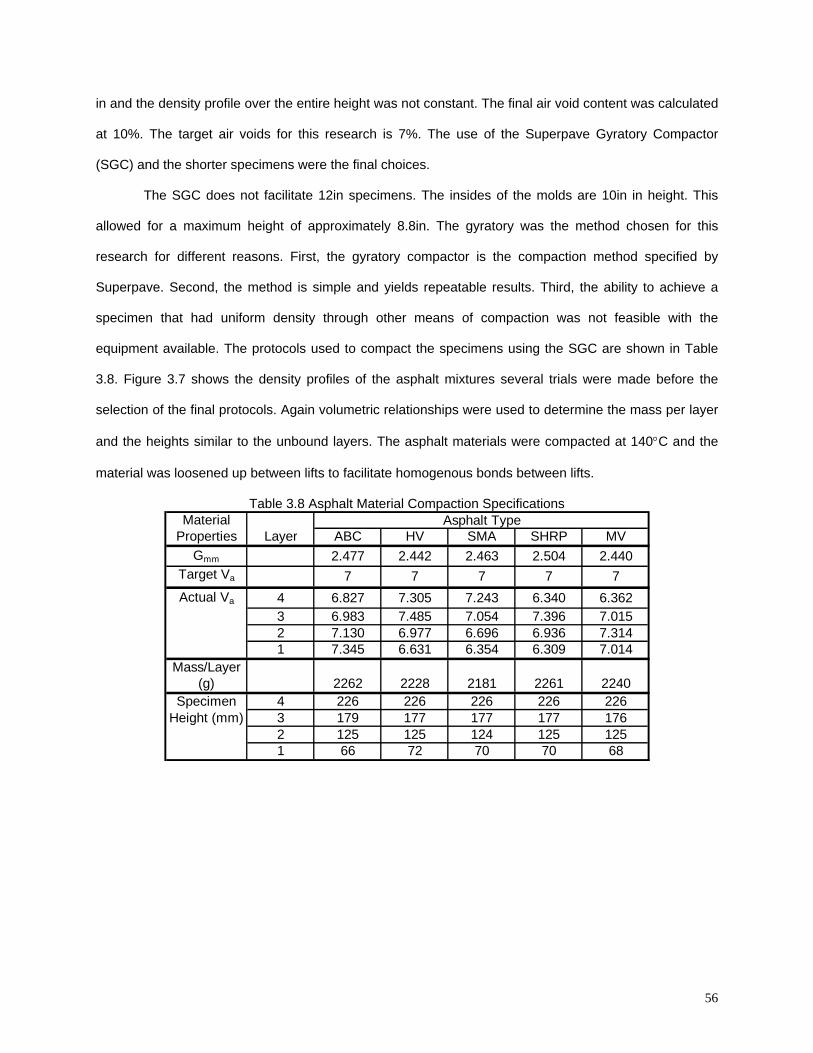
56
in and the density profile over the entire height was not constant. The final air void content was calculated
at 10%. The target air voids for this research is 7%. The use of the Superpave Gyratory Compactor
(SGC) and the shorter specimens were the final choices.
The SGC does not facilitate 12in specimens. The insides of the molds are 10in in height. This
allowed for a maximum height of approximately 8.8in. The gyratory was the method chosen for this
research for different reasons. First, the gyratory compactor is the compaction method specified by
Superpave. Second, the method is simple and yields repeatable results. Third, the ability to achieve a
specimen that had uniform density through other means of compaction was not feasible with the
equipment available. The protocols used to compact the specimens using the SGC are shown in Table
3.8. Figure 3.7 shows the density profiles of the asphalt mixtures several trials were made before the
selection of the final protocols. Again volumetric relationships were used to determine the mass per layer
and the heights similar to the unbound layers. The asphalt materials were compacted at 140°C and the
material was loosened up between lifts to facilitate homogenous bonds between lifts.
Table 3.8 Asphalt Material Compaction Specifications Material
Properties Layer ABC HV SMA SHRP MVGmm 2.477 2.442 2.463 2.504 2.440
Target Va 7 7 7 7 7Actual Va 4 6.827 7.305 7.243 6.340 6.362
3 6.983 7.485 7.054 7.396 7.0152 7.130 6.977 6.696 6.936 7.3141 7.345 6.631 6.354 6.309 7.014
Mass/Layer(g) 2262 2228 2181 2261 2240
Specimen 4 226 226 226 226 226Height (mm) 3 179 177 177 177 176
2 125 125 124 125 1251 66 72 70 70 68
Asphalt Type
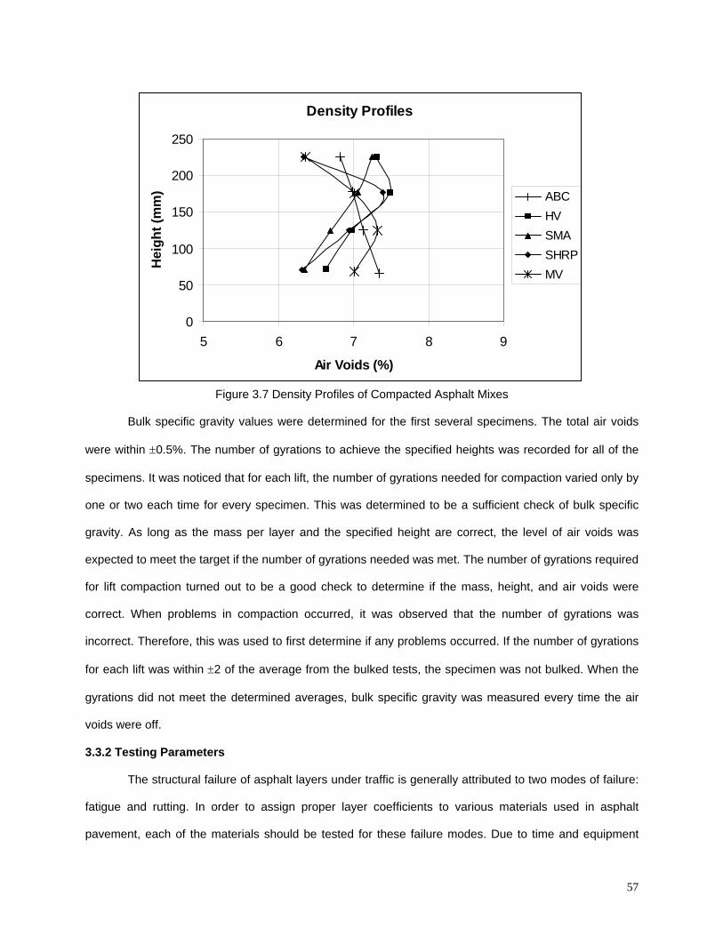
57
Density Profiles
0
50
100
150
200
250
5 6 7 8 9
Air Voids (%)
Hei
ght (
mm
) ABCHVSMASHRPMV
Figure 3.7 Density Profiles of Compacted Asphalt Mixes
Bulk specific gravity values were determined for the first several specimens. The total air voids
were within ±0.5%. The number of gyrations to achieve the specified heights was recorded for all of the
specimens. It was noticed that for each lift, the number of gyrations needed for compaction varied only by
one or two each time for every specimen. This was determined to be a sufficient check of bulk specific
gravity. As long as the mass per layer and the specified height are correct, the level of air voids was
expected to meet the target if the number of gyrations needed was met. The number of gyrations required
for lift compaction turned out to be a good check to determine if the mass, height, and air voids were
correct. When problems in compaction occurred, it was observed that the number of gyrations was
incorrect. Therefore, this was used to first determine if any problems occurred. If the number of gyrations
for each lift was within ±2 of the average from the bulked tests, the specimen was not bulked. When the
gyrations did not meet the determined averages, bulk specific gravity was measured every time the air
voids were off.
3.3.2 Testing Parameters
The structural failure of asphalt layers under traffic is generally attributed to two modes of failure:
fatigue and rutting. In order to assign proper layer coefficients to various materials used in asphalt
pavement, each of the materials should be tested for these failure modes. Due to time and equipment
58
limitations, the work in this thesis covers only rutting behavior. The rutting testing was conducted in a tri-
axial cell apparatus that is designed to create compressive stresses combined with some shearing action.
The resilient modulus was also investigated since this is the traditional method employed to determine
layer coefficients.
3.3.2.1 Unbound Material Parameters
The unbound granular material was tested at ambient temperature (22°C) on the assumption that
there is no freezing and the material drains adequately. Ambient temperatures are used because granular
materials are not generally dependent on temperature unless the water within them freezes.
The materials were tested at two moisture contents. Originally the moisture contents that
corresponded with the 95% density line drawn against the modified proctor results were used. For the 50-
50 material this corresponded with moisture contents of 1.8% and 10.4%. For the pulverized material the
moisture contents were 1.5% and 10.5%. The 95% of maximum density mark was chosen because this is
generally the density targeted in field construction. However, it was discovered early on in the testing that
the 10% moisture contents were too high. Results could not be generated due to rapid specimen failures.
The wet level moisture contents had to be dropped to 5%. This level generated completed tests and
repeatable results. The PCC-AC materials were tested in their dry conditions only.
As for resilient modulus testing, the AASHTO T294-94 (SHRP P46) specification was used. The
materials in this project fall into the type 1 soil category. All the specified confining pressures (σ B3B) and
deviator stresses (σ BdB) specified in AASHTO T294 were used in the testing.
The determination of σ B3 Band σ Bd Bapplied for the rutting tests was approached from two directions.
First σ B3B values needed to be established. This was first done by performing a wedge analysis under a
strip load to approximate the horizontal pressure at the edge of a loaded area. This assumes that rutting
occurs as a series of bearing capacity failures. This analysis generated a σ B3B of 52.4kPa. Confining
pressure was also checked under a circular flexible, uniformly loaded plate using elastic theory. This gave
a σ B3B of approximately 75kPa; it also suggested that at σ B3 Bmid-depth of an assumed 18” base course was
35kPa. From these analyses a starting σ B3B value of 34kPa (5psi) was used in a series of rutting step tests.
These tests used varying principle stress ratios (σ B1B/σ B3B) to determine the key stress parameters to use for
the final rutting tests. Three different load repetition values were tried: 100, 1000, and 10,000. From the
59
results of the trials, σ B1B/σ B3 Bratios of 2 and 4 were selected; when the ratio increased much above 4, the
specimens failed. The number of repetitions was set at 1000. It was noticed that the granular materials
stabilized after approximately 100 repetitions and that the increase in permanent deformation became
linear.
Once the σ B1B/σ B3 Bratios were established, a pavement analysis was performed using the
KENLAYER program. Actual pavement geometries were used in the analysis along with material
properties. The stresses calculated by KENLAYER ranged from 30kPa to 241kPa. The 85 P
thP percentile
was picked from this range, using the following tri-axial relationship
13 σσσ =+ d (46)
where
σ B3B = confining pressure
σ BdB = deviator stress
σ B1B = total axial stress.
From this relationship along with a σ B1B/σ B3 Bratio of 2, a high end σ B3B of 103kPa was determined. Finally, using
the σ B1B/σ B3 Bratios of 2 and 4, σ BdB values were established.
3.3.2.2 Asphalt Surface Course Parameters
The parameters for temperature, stress, and density were picked based upon the levels expected
in actual field conditions. A σ B3B equal to 103kPa with a σ B1B/σ B3B ratio of 4 was used so that comparisons with
the ABC materials could be made. However, the upper σ B1B/σ B3B ratio was raised to 5.4 to represent the
higher stress levels experienced by the surface layers. The higher total axial stress (σ B1B) was selected to
simulate a 553kPa (80psi) pressure.
The density issue was resolved by looking at field construction conditions. Since roads are
generally opened to traffic at 7% air voids, it was decided to mimic that level to better simulate field
conditions. The gyratory compactor was used to produce samples with a density of 93% G Bmm B.
Two temperatures were selected that would bracket the average high pavement surface
temperature of 58°C, which is commonly experienced in Wisconsin. A range of 12°C was chosen to
establish if there was any temperature effect and if so how severe the temperature effect is. Therefore, all
60
bound material rutting tests were conducted at 52°C and 64°C. The resilient modulus tests were
conducted at 20°C. This is the temperature that is traditionally used to derive layer coefficients from
resilient modulus data.
The rutting tests for the asphalt materials were run for 6000 cycles or 6% strain, which ever came
first. The 6% strain was considered as representative of pavement failure conditions. The number of
cycles was increased because of the visco-elastic nature of the material. The 6000 cycles were selected
to limit the time of testing with a reasonable time period. All of the testing parameters are presented in
Table 3.9.
As described previously ABC is a bound material. However, it is used as a base course rather
than a surface course. Therefore, a special protocol was established to include some of the testing
parameters used for granular materials and the parameters used for the bound materials.
This material is produced, transported, paved, and compacted like a surface asphalt mixture.
Surface mixes experience relatively high temperatures when manufactured as well as during their life
spans. To compare the ABC to the other mixes, the ABC was tested at the same temperatures as the
surface mixtures. Those temperatures and how they were determined are discussed in the next section.
Testing the ABC was done at some of the same stress conditions that the granular material was
tested at because the ABC will be in a lower layer of the asphalt pavement and, therefore, will naturally
experience lower stresses. One confining pressure was used: σ B3B= 103kPa, which is one of the stress
conditions used for testing the surface materials.
Resilient modulus tests for this material were conducted according to the AASHTO T294-94
(SHRP P46) specification. This is not the traditional testing method for resilient testing of asphalt
materials. Resilient modulus tests for asphalt materials are specified by ASTM D 4123-82 (1995), which
is an indirect tensile type test. The tri-axial M Br B was done because the rutting tests were performed in the
tri-axial apparatus and this method of testing better simulates the actual pavement loading, experienced
under traffic. Also, using the tri-axial method for both the rutting and resilient modulus tests would allow
for an easy comparison between the results from both tests. The MBr B test was conducted at both
temperatures used for the rutting tests as well as at 20°C. There was no deviation from the stress levels
specified by AASHTO T294-94.
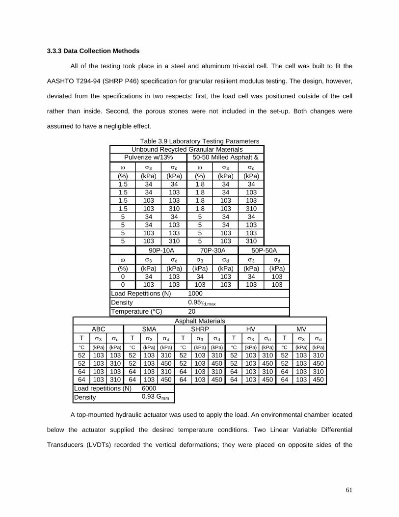
61
3.3.3 Data Collection Methods
All of the testing took place in a steel and aluminum tri-axial cell. The cell was built to fit the
AASHTO T294-94 (SHRP P46) specification for granular resilient modulus testing. The design, however,
deviated from the specifications in two respects: first, the load cell was positioned outside of the cell
rather than inside. Second, the porous stones were not included in the set-up. Both changes were
assumed to have a negligible effect.
Table 3.9 Laboratory Testing Parameters
ω σ3 σd ω σ3 σd
(%) (kPa) (kPa) (%) (kPa) (kPa)1.5 34 34 1.8 34 341.5 34 103 1.8 34 1031.5 103 103 1.8 103 1031.5 103 310 1.8 103 3105 34 34 5 34 345 34 103 5 34 1035 103 103 5 103 1035 103 310 5 103 310
ω σ3 σd σ3 σd σ3 σd
(%) (kPa) (kPa) (kPa) (kPa) (kPa) (kPa)0 34 103 34 103 34 1030 103 103 103 103 103 103
Load Repetitions (N) 1000Density 0.95γd,max
Temperature (°C) 20
Unbound Recycled Granular MaterialsPulverize w/13% 50-50 Milled Asphalt &
90P-10A 70P-30A 50P-50A
T σ3 σd T σ3 σd T σ3 σd T σ3 σd T σ3 σd
°C (kPa) (kPa) °C (kPa) (kPa) °C (kPa) (kPa) °C (kPa) (kPa) °C (kPa) (kPa)52 103 103 52 103 310 52 103 310 52 103 310 52 103 31052 103 310 52 103 450 52 103 450 52 103 450 52 103 45064 103 103 64 103 310 64 103 310 64 103 310 64 103 31064 103 310 64 103 450 64 103 450 64 103 450 64 103 450
Load repetitions (N) 6000Density 0.93 Gmm
Asphalt MaterialsABC SMA SHRP HV MV
A top-mounted hydraulic actuator was used to apply the load. An environmental chamber located
below the actuator supplied the desired temperature conditions. Two Linear Variable Differential
Transducers (LVDTs) recorded the vertical deformations; they were placed on opposite sides of the
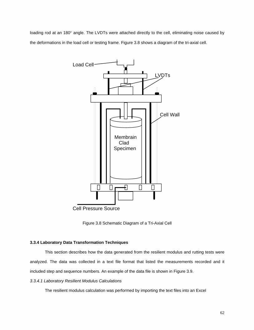
62
loading rod at an 180° angle. The LVDTs were attached directly to the cell, eliminating noise caused by
the deformations in the load cell or testing frame. Figure 3.8 shows a diagram of the tri-axial cell.
LVDTs
Load Cell
Cell Wall
MembrainClad
Specimen
Cell Pressure Source
Figure 3.8 Schematic Diagram of a Tri-Axial Cell
3.3.4 Laboratory Data Transformation Techniques
This section describes how the data generated from the resilient modulus and rutting tests were
analyzed. The data was collected in a text file format that listed the measurements recorded and it
included step and sequence numbers. An example of the data file is shown in Figure 3.9.
3.3.4.1 Laboratory Resilient Modulus Calculations
The resilient modulus calculation was performed by importing the text files into an Excel
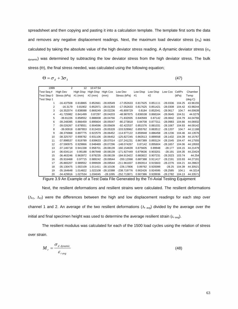
63
spreadsheet and then copying and pasting it into a calculation template. The template first sorts the data
and removes any negative displacement readings. Next, the maximum load deviator stress (σ BdB) was
calculated by taking the absolute value of the high deviator stress reading. A dynamic deviator stress (σ Bd
dynamic B) was determined by subtracting the low deviator stress from the high deviator stress. The bulk
stress (Θ), the final stress needed, was calculated using the following equation;
33σσ +=Θ d (47)
1999 2 12 10:47:54Test Seq.# High Dev High Disp High Disp High Cox Low Dev Low Disp Low Disp Low Cox CellPx Chamber Test Step 0 Stress (kPa) #1 (mm) #2 (mm) (mm) Stress (kPa) #1 #2 (kPa) TempTest Step 1 (deg C)
1 -16.437508 0.818865 0.852661 -28.00549 -17.052633 0.817625 0.851111 -28.0336 104.25 43.961552 -16.3179 0.81902 0.852971 -28.01393 -17.052633 0.817625 0.851421 -28.0308 104.42 43.982443 -16.352074 0.838088 0.869249 -28.02236 -45.809729 0.8184 0.852041 -28.0617 104.7 44.006394 -41.725982 0.841499 0.87297 -28.04203 -48.987875 0.836538 0.868164 -28.0645 104.51 44.02795 -39.81226 0.858552 0.888008 -28.04766 -71.832935 0.840569 0.87142 -28.0842 104.79 44.047666 -39.248395 0.866459 0.895604 -28.05047 -80.273818 0.84708 0.877311 -28.0983 104.66 44.069327 -39.026267 0.878551 0.904596 -28.05609 -92.422537 0.851576 0.881031 -28.1067 104.93 44.091428 -39.00918 0.887853 0.913433 -28.05328 -103.528962 0.855762 0.883512 -28.1207 104.7 44.111889 -38.376968 0.897775 0.922579 -28.06452 -114.977122 0.859948 0.886458 -28.1236 104.46 44.13576
10 -38.325707 0.908782 0.931106 -28.06452 -125.827245 0.863513 0.889558 -28.1432 104.39 44.1576711 -37.898537 0.919789 0.939633 -28.07014 -137.241231 0.867389 0.893124 -28.1545 104.47 44.1755512 -37.590975 0.929866 0.948469 -28.07296 -148.074267 0.87142 0.895604 -28.1657 104.06 44.1959313 -37.146718 0.941338 0.958701 -28.08139 -160.154639 0.875605 0.89948 -28.177 104.15 44.2147914 -36.634114 0.95188 0.967848 -28.08139 -171.927449 0.879636 0.903201 -28.191 104.35 44.2342415 -36.463246 0.963972 0.978235 -28.08139 -184.913422 0.883822 0.907231 -28.2023 103.74 44.25416 -35.916468 0.97715 0.989242 -28.09544 -200.12068 0.887388 0.911417 -28.2191 103.93 44.2719117 -35.865207 0.989552 0.999939 -28.09544 -211.961837 0.892814 0.915603 -28.2276 104.21 44.2882218 -35.130475 1.002109 1.011411 -28.10106 -226.17806 0.89762 0.920099 -28.25 104.39 44.3052119 -35.164648 1.014822 1.022108 -28.10388 -238.719776 0.902426 0.924595 -28.2585 104.1 44.321420 -34.429916 1.027534 1.034045 -28.1095 -252.713871 0.907386 0.928936 -28.2782 104.13 44.33571
Figure 3.9 An Example of a Test Data File Generated by the Tri-Axial Testing Equipment
Next, the resilient deformations and resilient strains were calculated. The resilient deformations
(∆ Br1B, ∆ Br2B) were the differences between the high and low displacement readings for each step over
channel 1 and 2. An average of the two resilient deformations (∆Br avgB) divided by the average over the
initial and final specimen height was used to determine the average resilient strain (εBr avgB).
The resilient modulus was calculated for each of the 1500 load cycles using the relation of stress
over strain.
avgr
dynamicdrM
εσ
= (48)
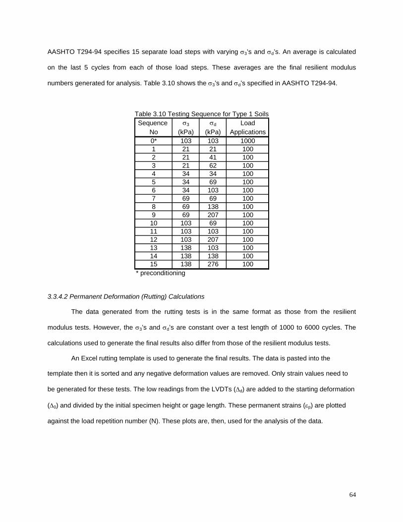
64
AASHTO T294-94 specifies 15 separate load steps with varying σ B3B’s and σ BdB’s. An average is calculated
on the last 5 cycles from each of those load steps. These averages are the final resilient modulus
numbers generated for analysis. Table 3.10 shows the σ B3B’s and σ BdB’s specified in AASHTO T294-94.
Table 3.10 Testing Sequence for Type 1 Soils Sequence σ3 σd Load
No (kPa) (kPa) Applications0* 103 103 10001 21 21 1002 21 41 1003 21 62 1004 34 34 1005 34 69 1006 34 103 1007 69 69 1008 69 138 1009 69 207 100
10 103 69 10011 103 103 10012 103 207 10013 138 103 10014 138 138 10015 138 276 100
* preconditioning
3.3.4.2 Permanent Deformation (Rutting) Calculations
The data generated from the rutting tests is in the same format as those from the resilient
modulus tests. However, the σ B3B’s and σ BdB’s are constant over a test length of 1000 to 6000 cycles. The
calculations used to generate the final results also differ from those of the resilient modulus tests.
An Excel rutting template is used to generate the final results. The data is pasted into the
template then it is sorted and any negative deformation values are removed. Only strain values need to
be generated for these tests. The low readings from the LVDTs (∆BdB) are added to the starting deformation
(∆ B0B) and divided by the initial specimen height or gage length. These permanent strains (εBpB) are plotted
against the load repetition number (N). These plots are, then, used for the analysis of the data.
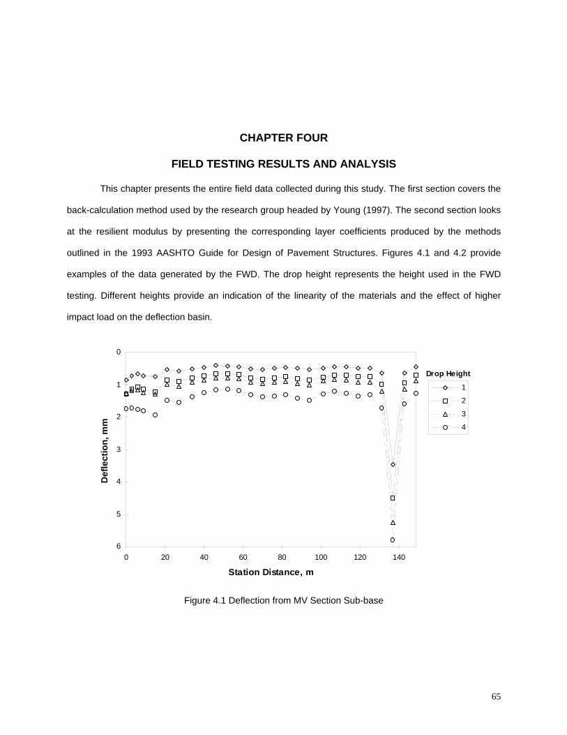
CHAPTER FOUR
FIELD TESTING RESULTS AND ANALYSIS
This chapter presents the entire field data collected during this study. The first section covers the
back-calculation method used by the research group headed by Young (1997). The second section looks
at the resilient modulus by presenting the corresponding layer coefficients produced by the methods
outlined in the 1993 AASHTO Guide for Design of Pavement Structures. Figures 4.1 and 4.2 provide
examples of the data generated by the FWD. The drop height represents the height used in the FWD
testing. Different heights provide an indication of the linearity of the materials and the effect of higher
impact load on the deflection basin.
0
1
2
3
4
5
60 20 40 60 80 100 120 140
Station Distance, m
1
2
3
4
Drop Height
Def
lect
ion,
mm
Figure 4.1 Deflection from MV Section Sub-base
65
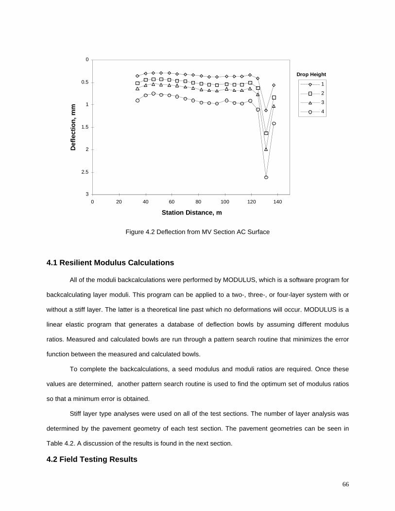
0
0.5
1
1.5
2
2.5
30 20 40 60 80 100 120 140
Station Distance, m
1
2
3
4
Drop HeightD
efle
ctio
n, m
m
Figure 4.2 Deflection from MV Section AC Surface
4.1 Resilient Modulus Calculations
All of the moduli backcalculations were performed by MODULUS, which is a software program for
backcalculating layer moduli. This program can be applied to a two-, three-, or four-layer system with or
without a stiff layer. The latter is a theoretical line past which no deformations will occur. MODULUS is a
linear elastic program that generates a database of deflection bowls by assuming different modulus
ratios. Measured and calculated bowls are run through a pattern search routine that minimizes the error
function between the measured and calculated bowls.
To complete the backcalculations, a seed modulus and moduli ratios are required. Once these
values are determined, another pattern search routine is used to find the optimum set of modulus ratios
so that a minimum error is obtained.
Stiff layer type analyses were used on all of the test sections. The number of layer analysis was
determined by the pavement geometry of each test section. The pavement geometries can be seen in
Table 4.2. A discussion of the results is found in the next section.
4.2 Field Testing Results
66
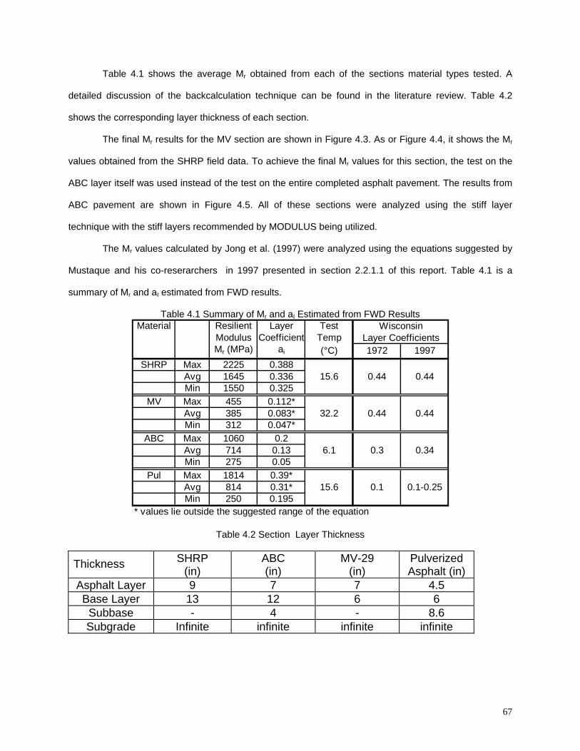
Table 4.1 shows the average Mr obtained from each of the sections material types tested. A
detailed discussion of the backcalculation technique can be found in the literature review. Table 4.2
shows the corresponding layer thickness of each section.
The final Mr results for the MV section are shown in Figure 4.3. As or Figure 4.4, it shows the Mr
values obtained from the SHRP field data. To achieve the final Mr values for this section, the test on the
ABC layer itself was used instead of the test on the entire completed asphalt pavement. The results from
ABC pavement are shown in Figure 4.5. All of these sections were analyzed using the stiff layer
technique with the stiff layers recommended by MODULUS being utilized.
The Mr values calculated by Jong et al. (1997) were analyzed using the equations suggested by
Mustaque and his co-reserarchers in 1997 presented in section 2.2.1.1 of this report. Table 4.1 is a
summary of Mr and aI estimated from FWD results.
Table 4.1 Summary of Mr and aI Estimated from FWD Results Material Resilient Layer Test
Modulus Coefficient TempMr (MPa) ai (°C) 1972 1997
SHRP Max 2225 0.388Avg 1645 0.336 15.6 0.44 0.44Min 1550 0.325
MV Max 455 0.112*Avg 385 0.083* 32.2 0.44 0.44Min 312 0.047*
ABC Max 1060 0.2Avg 714 0.13 6.1 0.3 0.34Min 275 0.05
Pul Max 1814 0.39*Avg 814 0.31* 15.6 0.1 0.1-0.25Min 250 0.195
* values lie outside the suggested range of the equation
Wisconsin Layer Coefficients
Table 4.2 Section Layer Thickness
Thickness SHRP (in)
ABC (in)
MV-29 (in)
Pulverized Asphalt (in)
Asphalt Layer 9 7 7 4.5 Base Layer 13 12 6 6
Subbase - 4 - 8.6 Subgrade Infinite infinite infinite infinite
67
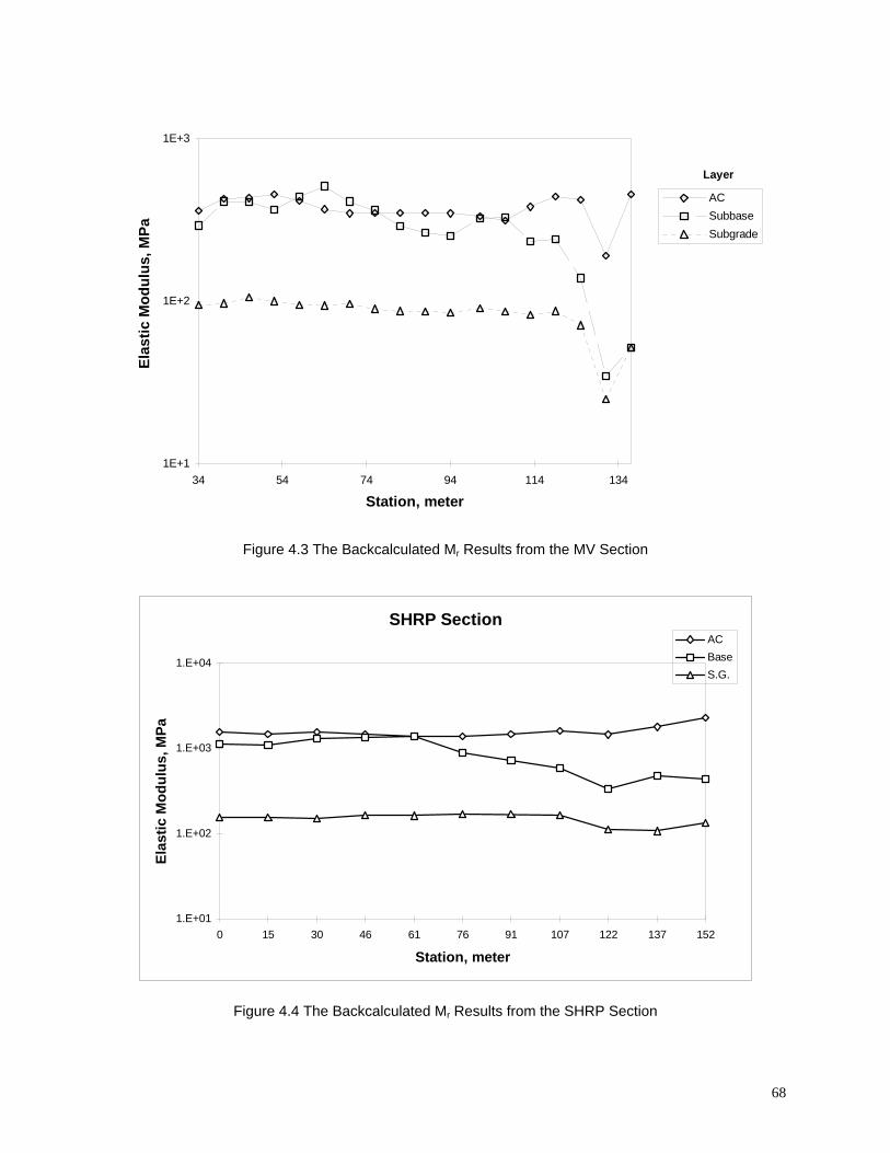
1E+1
1E+2
1E+3
34 54 74 94 114 134
Station, meter
ACSubbaseSubgrade
Layer
Elas
tic M
odul
us, M
Pa
Figure 4.3 The Backcalculated Mr Results from the MV Section
SHRP Section
1.E+01
1.E+02
1.E+03
1.E+04
0 15 30 46 61 76 91 107 122 137 152
Station, meter
Elas
tic M
odul
us, M
Pa
ACBaseS.G.
Figure 4.4 The Backcalculated Mr Results from the SHRP Section
68
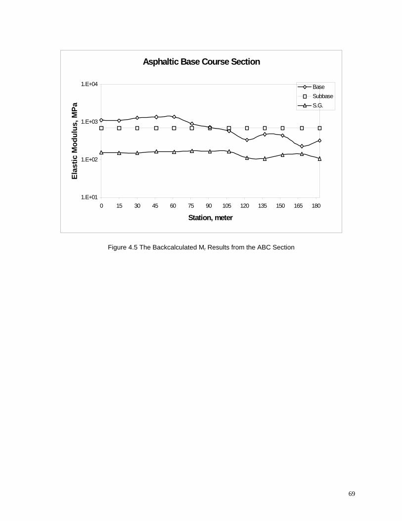
Asphaltic Base Course Section
1.E+01
1.E+02
1.E+03
1.E+04
0 15 30 45 60 75 90 105 120 135 150 165 180
Station, meter
Elas
tic M
odul
us, M
PaBaseSubbaseS.G.
Figure 4.5 The Backcalculated Mr Results from the ABC Section
69
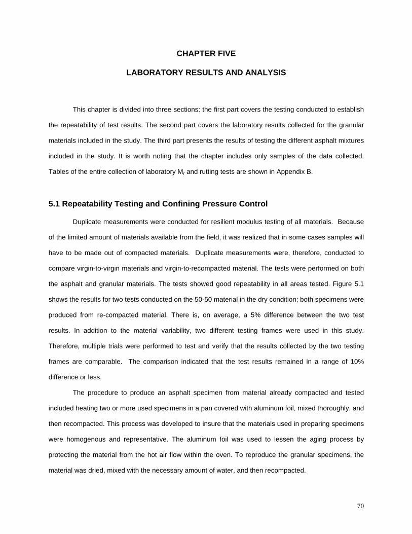
CHAPTER FIVE
LABORATORY RESULTS AND ANALYSIS
This chapter is divided into three sections: the first part covers the testing conducted to establish
the repeatability of test results. The second part covers the laboratory results collected for the granular
materials included in the study. The third part presents the results of testing the different asphalt mixtures
included in the study. It is worth noting that the chapter includes only samples of the data collected.
Tables of the entire collection of laboratory Mr and rutting tests are shown in Appendix B.
5.1 Repeatability Testing and Confining Pressure Control
Duplicate measurements were conducted for resilient modulus testing of all materials. Because
of the limited amount of materials available from the field, it was realized that in some cases samples will
have to be made out of compacted materials. Duplicate measurements were, therefore, conducted to
compare virgin-to-virgin materials and virgin-to-recompacted material. The tests were performed on both
the asphalt and granular materials. The tests showed good repeatability in all areas tested. Figure 5.1
shows the results for two tests conducted on the 50-50 material in the dry condition; both specimens were
produced from re-compacted material. There is, on average, a 5% difference between the two test
results. In addition to the material variability, two different testing frames were used in this study.
Therefore, multiple trials were performed to test and verify that the results collected by the two testing
frames are comparable. The comparison indicated that the test results remained in a range of 10%
difference or less.
The procedure to produce an asphalt specimen from material already compacted and tested
included heating two or more used specimens in a pan covered with aluminum foil, mixed thoroughly, and
then recompacted. This process was developed to insure that the materials used in preparing specimens
were homogenous and representative. The aluminum foil was used to lessen the aging process by
protecting the material from the hot air flow within the oven. To reproduce the granular specimens, the
material was dried, mixed with the necessary amount of water, and then recompacted.
70
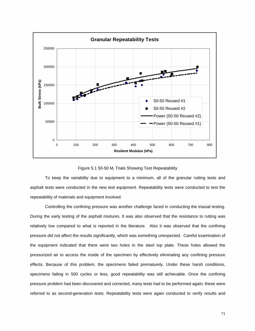
Granular Repeatability Tests
0
50000
100000
150000
200000
250000
0 100 200 300 400 500 600 700 800
Resilient Modulus (kPa)
Bul
k St
ress
(kPa
)
50-50 Reused #1
50-50 Reused #2
Power (50-50 Reused #2)
Power (50-50 Reused #1)
Figure 5.1 50-50 Mr Trials Showing Test Repeatability
To keep the variability due to equipment to a minimum, all of the granular rutting tests and
asphalt tests were conducted in the new test equipment. Repeatability tests were conducted to test the
repeatability of materials and equipment involved.
Controlling the confining pressure was another challenge faced in conducting the triaxial testing.
During the early testing of the asphalt mixtures. It was also observed that the resistance to rutting was
relatively low compared to what is reported in the literature. Also it was observed that the confining
pressure did not affect the results significantly, which was something unexpected. Careful examination of
the equipment indicated that there were two holes in the steel top plate. These holes allowed the
pressurized air to access the inside of the specimen by effectively eliminating any confining pressure
effects. Because of this problem, the specimens failed prematurely. Under these harsh conditions,
specimens failing in 500 cycles or less, good repeatability was still achievable. Once the confining
pressure problem had been discovered and corrected, many tests had to be performed again; these were
referred to as second-generation tests. Repeatability tests were again conducted to verify results and
71
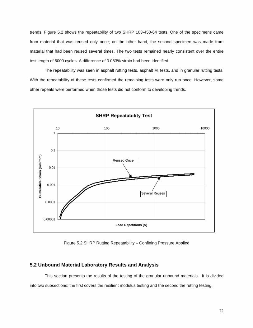
trends. Figure 5.2 shows the repeatability of two SHRP 103-450-64 tests. One of the specimens came
from material that was reused only once; on the other hand, the second specimen was made from
material that had been reused several times. The two tests remained nearly consistent over the entire
test length of 6000 cycles. A difference of 0.063% strain had been identified.
The repeatability was seen in asphalt rutting tests, asphalt Mr tests, and in granular rutting tests.
With the repeatability of these tests confirmed the remaining tests were only run once. However, some
other repeats were performed when those tests did not conform to developing trends.
SHRP Repeatability Test
0.00001
0.0001
0.001
0.01
0.1
110 100 1000 10000
Load Repetitions (N)
Cum
ulat
ive
Stra
in (m
m/m
m)
Reused Once
Several Reuses
Figure 5.2 SHRP Rutting Repeatability – Confining Pressure Applied
5.2 Unbound Material Laboratory Results and Analysis
This section presents the results of the testing of the granular unbound materials. It is divided
into two subsections: the first covers the resilient modulus testing and the second the rutting testing.
72
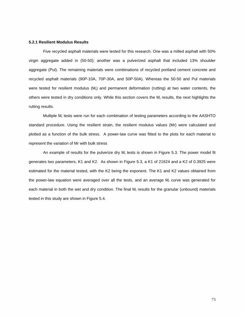
5.2.1 Resilient Modulus Results
Five recycled asphalt materials were tested for this research. One was a milled asphalt with 50%
virgin aggregate added in (50-50); another was a pulverized asphalt that included 13% shoulder
aggregate (Pul). The remaining materials were combinations of recycled portland cement concrete and
recycled asphalt materials (90P-10A, 70P-30A, and 50P-50A). Whereas the 50-50 and Pul materials
were tested for resilient modulus (Mr) and permanent deformation (rutting) at two water contents, the
others were tested in dry conditions only. While this section covers the Mr results, the next highlights the
rutting results.
Multiple Mr tests were run for each combination of testing parameters according to the AASHTO
standard procedure. Using the resilient strain, the resilient modulus values (Mr) were calculated and
plotted as a function of the bulk stress. A power-law curve was fitted to the plots for each material to
represent the variation of Mr with bulk stress
An example of results for the pulverize dry Mr tests is shown in Figure 5.3. The power model fit
generates two parameters, K1 and K2. As shown in Figure 5.3, a K1 of 21624 and a K2 of 0.3925 were
estimated for the material tested, with the K2 being the exponent. The K1 and K2 values obtained from
the power-law equation were averaged over all the tests, and an average Mr curve was generated for
each material in both the wet and dry condition. The final Mr results for the granular (unbound) materials
tested in this study are shown in Figure 5.4.
73
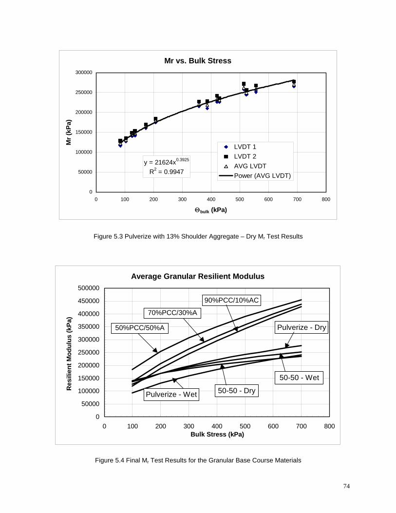
74
Mr vs. Bulk Stress
y = 21624x0.3925
R2 = 0.9947
0
50000
100000
150000
200000
250000
300000
0 100 200 300 400 500 600 700 800
Θbulk (kPa)
Mr (
kPa)
LVDT 1LVDT 2AVG LVDTPower (AVG LVDT)
Figure 5.3 Pulverize with 13% Shoulder Aggregate – Dry M Br B Test Results
Average Granular Resilient Modulus
0
50000
100000
150000
200000
250000
300000
350000
400000
450000
500000
0 100 200 300 400 500 600 700 800Bulk Stress (kPa)
Res
ilien
t Mod
ulus
(kPa
)
Pulverize - Dry
Pulverize - Wet
50-50 - Wet
50-50 - Dry
70%PCC/30%A
90%PCC/10%AC
50%PCC/50%A
Figure 5.4 Final M Br B Test Results for the Granular Base Course Materials
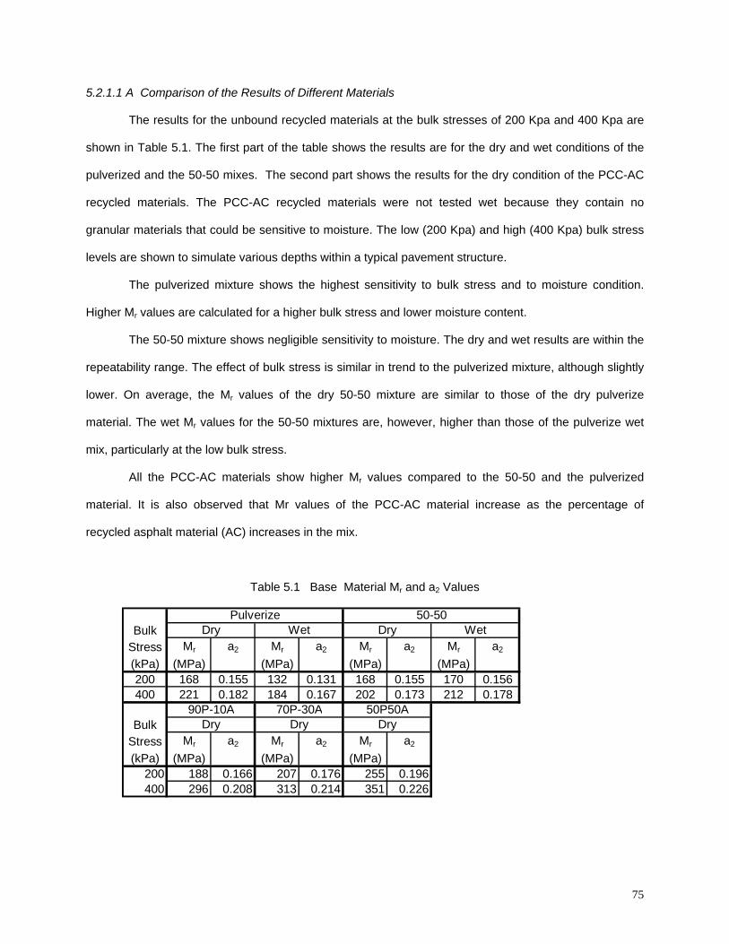
5.2.1.1 A Comparison of the Results of Different Materials
The results for the unbound recycled materials at the bulk stresses of 200 Kpa and 400 Kpa are
shown in Table 5.1. The first part of the table shows the results are for the dry and wet conditions of the
pulverized and the 50-50 mixes. The second part shows the results for the dry condition of the PCC-AC
recycled materials. The PCC-AC recycled materials were not tested wet because they contain no
granular materials that could be sensitive to moisture. The low (200 Kpa) and high (400 Kpa) bulk stress
levels are shown to simulate various depths within a typical pavement structure.
The pulverized mixture shows the highest sensitivity to bulk stress and to moisture condition.
Higher Mr values are calculated for a higher bulk stress and lower moisture content.
The 50-50 mixture shows negligible sensitivity to moisture. The dry and wet results are within the
repeatability range. The effect of bulk stress is similar in trend to the pulverized mixture, although slightly
lower. On average, the Mr values of the dry 50-50 mixture are similar to those of the dry pulverize
material. The wet Mr values for the 50-50 mixtures are, however, higher than those of the pulverize wet
mix, particularly at the low bulk stress.
All the PCC-AC materials show higher Mr values compared to the 50-50 and the pulverized
material. It is also observed that Mr values of the PCC-AC material increase as the percentage of
recycled asphalt material (AC) increases in the mix.
Table 5.1 Base Material Mr and a2 Values
BulkStress Mr a2 Mr a2 Mr a2 Mr a2
(kPa) (MPa) (MPa) (MPa) (MPa)200 168 0.155 132 0.131 168 0.155 170 0.156400 221 0.182 184 0.167 202 0.173 212 0.178
BulkStress Mr a2 Mr a2 Mr a2
(kPa) (MPa) (MPa) (MPa)200 188 0.166 207 0.176 255 0.196400 296 0.208 313 0.214 351 0.226
Dry Dry Dry90P-10A 70P-30A 50P50A
Pulverize 50-50Dry Wet Dry Wet
75
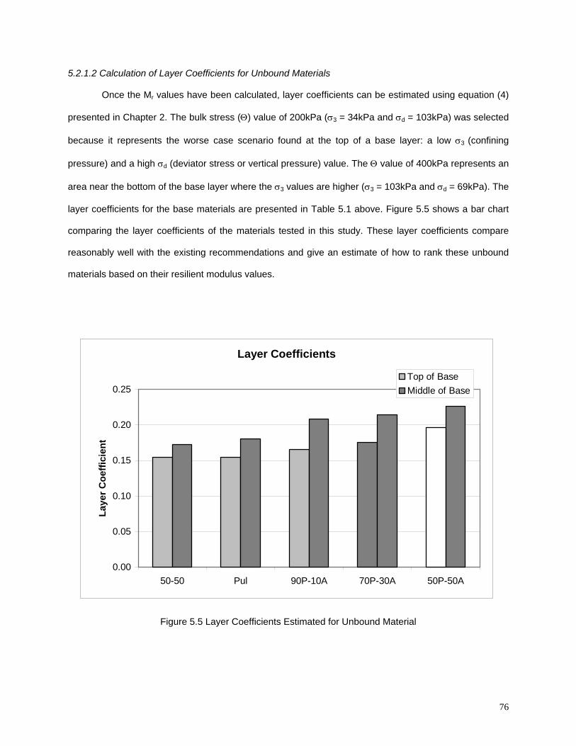
76
5.2.1.2 Calculation of Layer Coefficients for Unbound Materials
Once the MBr B values have been calculated, layer coefficients can be estimated using equation (4)
presented in Chapter 2. The bulk stress (Θ) value of 200kPa (σ B3B = 34kPa and σ BdB = 103kPa) was selected
because it represents the worse case scenario found at the top of a base layer: a low σ B3 B(confining
pressure) and a high σ BdB (deviator stress or vertical pressure) value. The Θ value of 400kPa represents an
area near the bottom of the base layer where the σ B3B values are higher (σ B3B = 103kPa and σ BdB = 69kPa). The
layer coefficients for the base materials are presented in Table 5.1 above. Figure 5.5 shows a bar chart
comparing the layer coefficients of the materials tested in this study. These layer coefficients compare
reasonably well with the existing recommendations and give an estimate of how to rank these unbound
materials based on their resilient modulus values.
Layer Coefficients
0.00
0.05
0.10
0.15
0.20
0.25
50-50 Pul 90P-10A 70P-30A 50P-50A
Laye
r Coe
ffici
ent
Top of BaseMiddle of Base
Figure 5.5 Layer Coefficients Estimated for Unbound Material
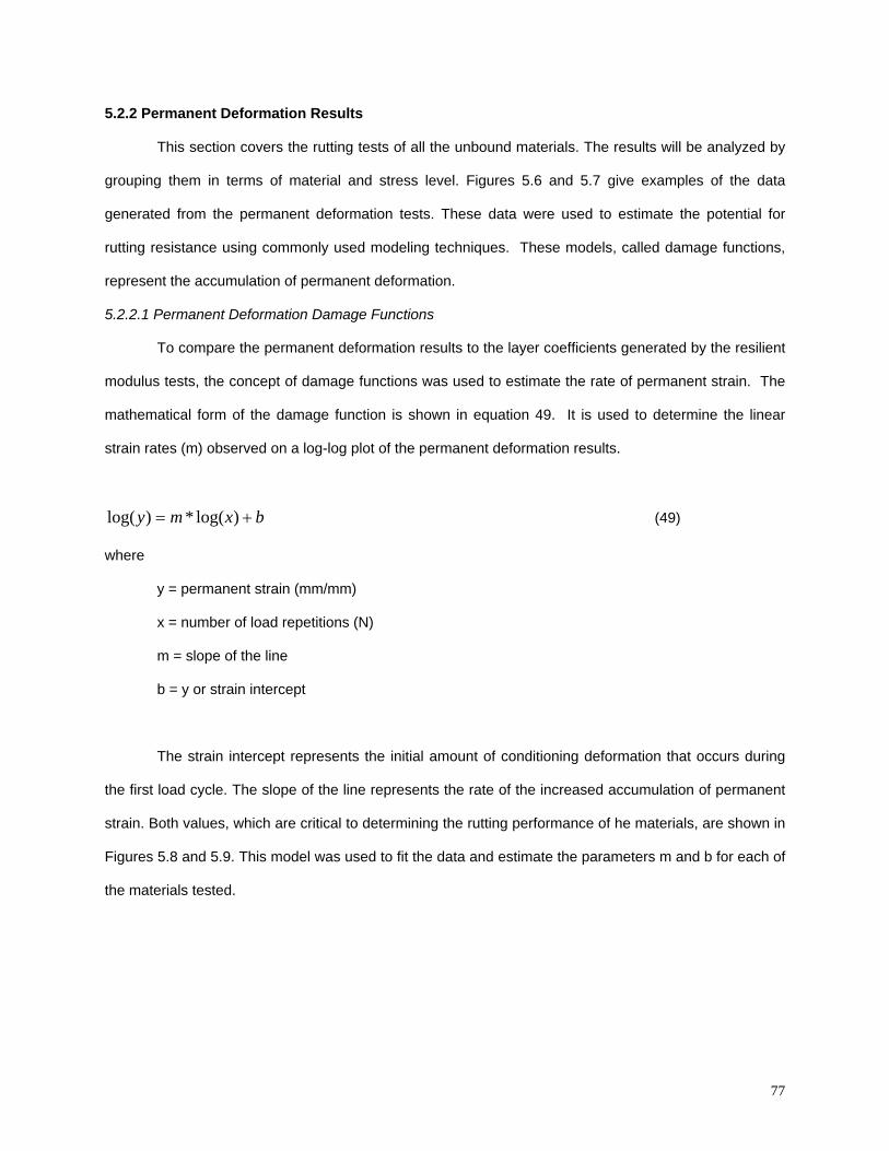
77
5.2.2 Permanent Deformation Results
This section covers the rutting tests of all the unbound materials. The results will be analyzed by
grouping them in terms of material and stress level. Figures 5.6 and 5.7 give examples of the data
generated from the permanent deformation tests. These data were used to estimate the potential for
rutting resistance using commonly used modeling techniques. These models, called damage functions,
represent the accumulation of permanent deformation.
5.2.2.1 Permanent Deformation Damage Functions
To compare the permanent deformation results to the layer coefficients generated by the resilient
modulus tests, the concept of damage functions was used to estimate the rate of permanent strain. The
mathematical form of the damage function is shown in equation 49. It is used to determine the linear
strain rates (m) observed on a log-log plot of the permanent deformation results.
bxmy += )log(*)log( (49)
where
y = permanent strain (mm/mm)
x = number of load repetitions (N)
m = slope of the line
b = y or strain intercept
The strain intercept represents the initial amount of conditioning deformation that occurs during
the first load cycle. The slope of the line represents the rate of the increased accumulation of permanent
strain. Both values, which are critical to determining the rutting performance of he materials, are shown in
Figures 5.8 and 5.9. This model was used to fit the data and estimate the parameters m and b for each of
the materials tested.
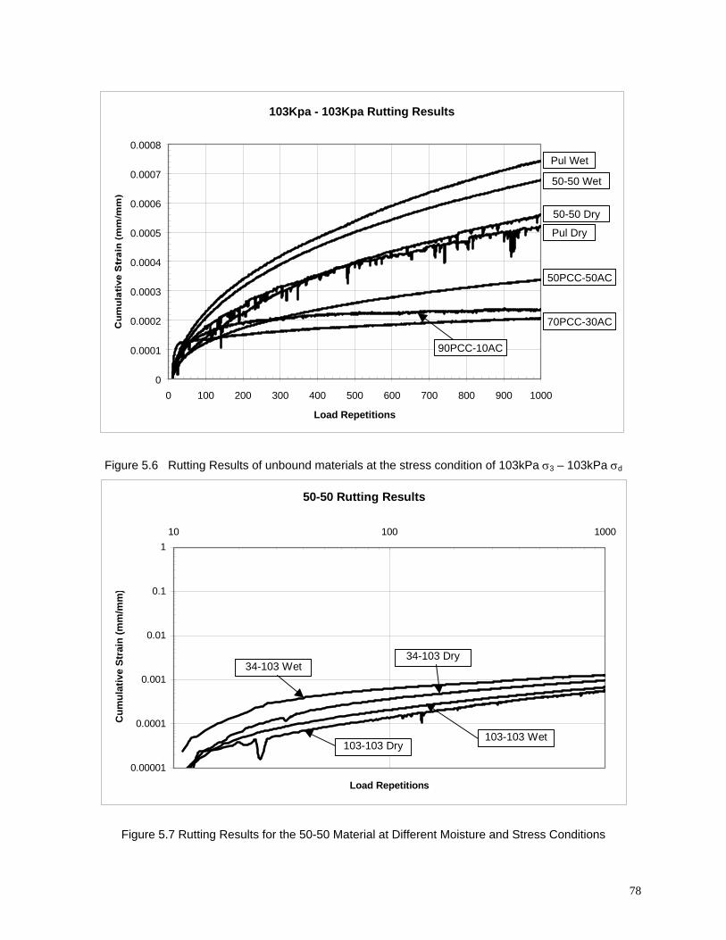
78
103Kpa - 103Kpa Rutting Results
0
0.0001
0.0002
0.0003
0.0004
0.0005
0.0006
0.0007
0.0008
0 100 200 300 400 500 600 700 800 900 1000
Load Repetitions
50-50 Wet
50-50 Dry
Pul Wet
Pul Dry
90PCC-10AC
50PCC-50AC
70PCC-30AC
Figure 5.6 Rutting Results of unbound materials at the stress condition of 103kPa σ B3B – 103kPa σ BdB
50-50 Rutting Results
0.00001
0.0001
0.001
0.01
0.1
110 100 1000
Load Repetitions
Cum
ulat
ive
Stra
in (m
m/m
m)
34-103 Wet
103-103 Wet103-103 Dry
34-103 Dry
Figure 5.7 Rutting Results for the 50-50 Material at Different Moisture and Stress Conditions
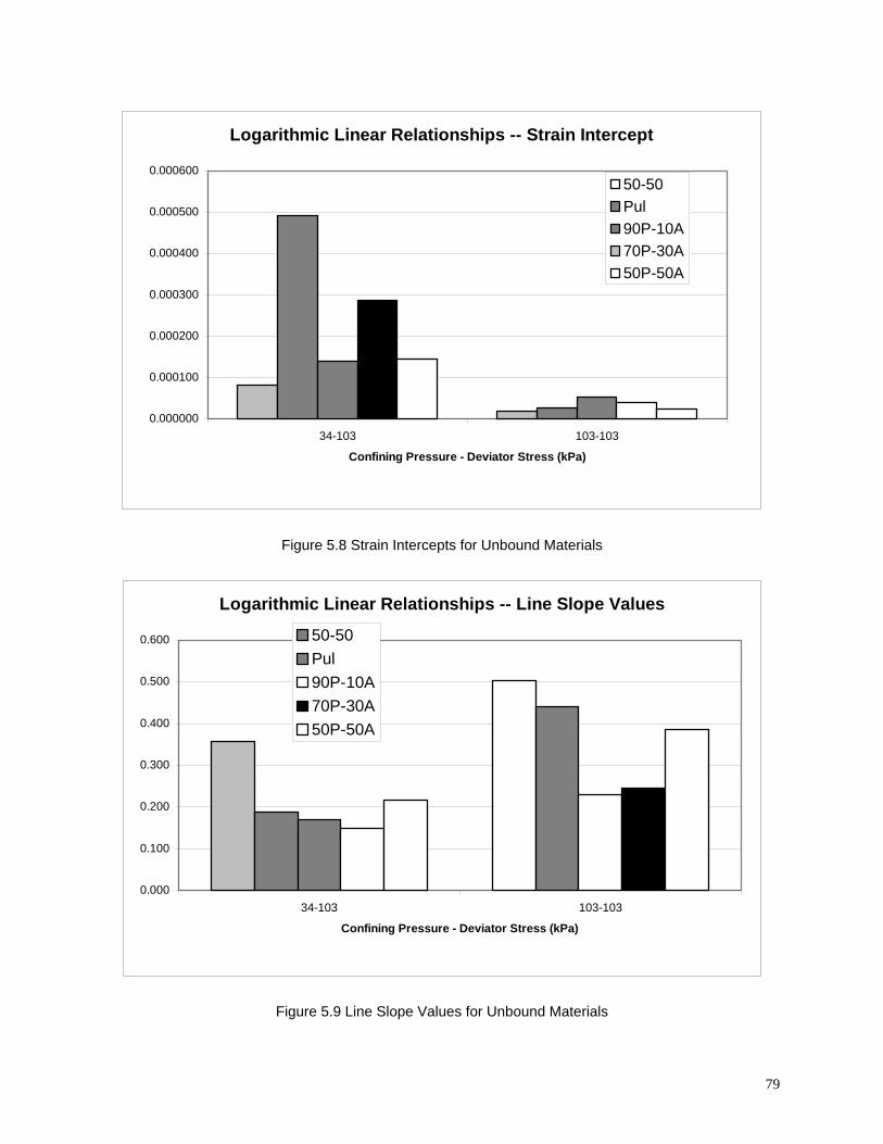
Logarithmic Linear Relationships -- Strain Intercept
0.000000
0.000100
0.000200
0.000300
0.000400
0.000500
0.000600
34-103 103-103
Confining Pressure - Deviator Stress (kPa)
50-50Pul90P-10A70P-30A50P-50A
Figure 5.8 Strain Intercepts for Unbound Materials
Logarithmic Linear Relationships -- Line Slope Values
0.000
0.100
0.200
0.300
0.400
0.500
0.600
34-103 103-103
Confining Pressure - Deviator Stress (kPa)
50-50Pul90P-10A70P-30A50P-50A
Figure 5.9 Line Slope Values for Unbound Materials
79
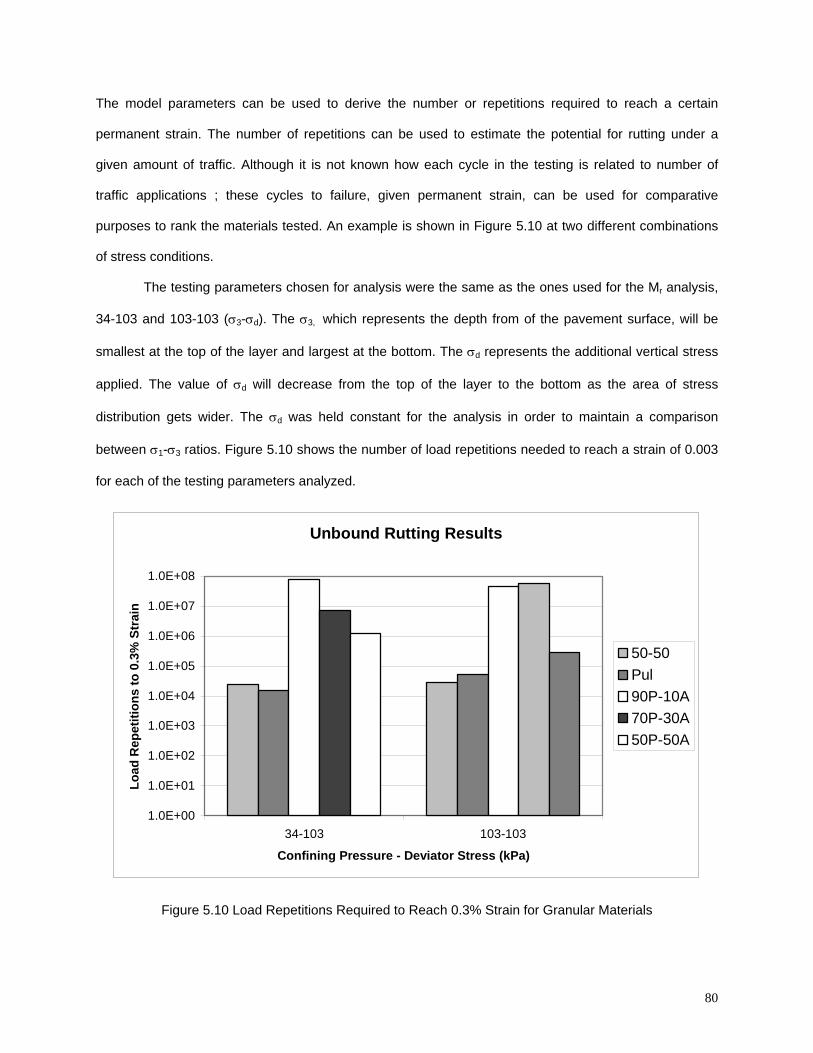
80
The model parameters can be used to derive the number or repetitions required to reach a certain
permanent strain. The number of repetitions can be used to estimate the potential for rutting under a
given amount of traffic. Although it is not known how each cycle in the testing is related to number of
traffic applications ; these cycles to failure, given permanent strain, can be used for comparative
purposes to rank the materials tested. An example is shown in Figure 5.10 at two different combinations
of stress conditions.
The testing parameters chosen for analysis were the same as the ones used for the MBr B analysis,
34-103 and 103-103 (σ B3B-σ BdB). The σ B3, Bwhich represents the depth from of the pavement surface, will be
smallest at the top of the layer and largest at the bottom. The σ BdB represents the additional vertical stress
applied. The value of σ BdB will decrease from the top of the layer to the bottom as the area of stress
distribution gets wider. The σ BdB was held constant for the analysis in order to maintain a comparison
between σ B1B-σ B3B ratios. Figure 5.10 shows the number of load repetitions needed to reach a strain of 0.003
for each of the testing parameters analyzed.
Unbound Rutting Results
1.0E+00
1.0E+01
1.0E+02
1.0E+03
1.0E+04
1.0E+05
1.0E+06
1.0E+07
1.0E+08
34-103 103-103
Confining Pressure - Deviator Stress (kPa)
Load
Rep
etiti
ons
to 0
.3%
Str
ain
50-50Pul90P-10A70P-30A50P-50A
Figure 5.10 Load Repetitions Required to Reach 0.3% Strain for Granular Materials
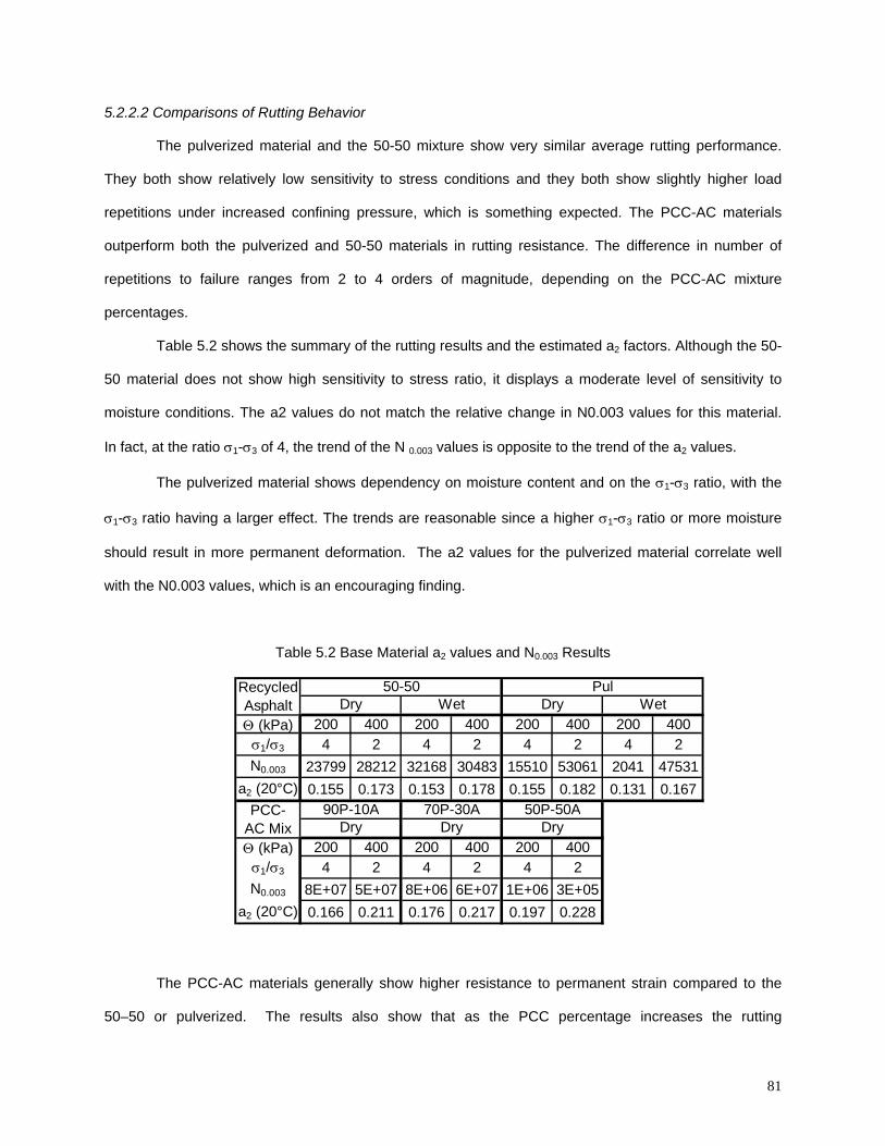
81
5.2.2.2 Comparisons of Rutting Behavior
The pulverized material and the 50-50 mixture show very similar average rutting performance.
They both show relatively low sensitivity to stress conditions and they both show slightly higher load
repetitions under increased confining pressure, which is something expected. The PCC-AC materials
outperform both the pulverized and 50-50 materials in rutting resistance. The difference in number of
repetitions to failure ranges from 2 to 4 orders of magnitude, depending on the PCC-AC mixture
percentages.
Table 5.2 shows the summary of the rutting results and the estimated aB2B factors. Although the 50-
50 material does not show high sensitivity to stress ratio, it displays a moderate level of sensitivity to
moisture conditions. The a2 values do not match the relative change in N0.003 values for this material.
In fact, at the ratio σ B1B-σ B3B of 4, the trend of the N B0.003B values is opposite to the trend of the a B2B values.
The pulverized material shows dependency on moisture content and on the σ B1B-σ B3B ratio, with the
σ B1B-σ B3B ratio having a larger effect. The trends are reasonable since a higher σ B1B-σ B3B ratio or more moisture
should result in more permanent deformation. The a2 values for the pulverized material correlate well
with the N0.003 values, which is an encouraging finding.
Table 5.2 Base Material a B2B values and N B0.003 B Results
RecycledAsphaltΘ (kPa) 200 400 200 400 200 400 200 400
σ1/σ3 4 2 4 2 4 2 4 2N0.003 23799 28212 32168 30483 15510 53061 2041 47531
a2 (20°C) 0.155 0.173 0.153 0.178 0.155 0.182 0.131 0.167PCC-
AC MixΘ (kPa) 200 400 200 400 200 400
σ1/σ3 4 2 4 2 4 2N0.003 8E+07 5E+07 8E+06 6E+07 1E+06 3E+05
a2 (20°C) 0.166 0.211 0.176 0.217 0.197 0.228
90P-10A 70P-30A 50P-50ADry Dry Dry
50-50 PulDry Wet Dry Wet
The PCC-AC materials generally show higher resistance to permanent strain compared to the
50–50 or pulverized. The results also show that as the PCC percentage increases the rutting

82
performance becomes more favorable. This trend is in opposition to the MBr B trend, which exhibits higher MBr B
values when the AC percentage increases. The only exception which deviates from this trend is the 70P-
30A material tested at 103-103. The PCC-AC mixtures show some dependence on σ B1B-σ B3B but this
dependence is opposition to the trend seen in the recycled asphalt material results. With the exception of
the 70P-30A, the amount of load repetitions to 0.3% strain decreases as the σ B1B-σ B3B ratio decreases.
The trend in the N0.003 data does not match the trend in the values of the a2 values. The lowest
a2 value corresponds to the highest N0.003 value for all the combinations of the PCC-AC materials.
5.2.2.3 Deriving the aB2B Values
Table 5.2 shows the comparisons between the M Br B a B2B values established from M Br B and the N B0.003B
results. It is clear that the a B2B values and the N0.003 values are sensitive to moisture, σ B1B-σ B3B ratio, and
material type. It is also observed that the a2 and N0.003 values do not correlate very well.
These results are not surprising since the moisture and σ B1B-σ B3B ratio are known to have an effect on
performance. In addition, the a2 values are derived directly from the resilient modulus, which is a
measure of resilient non-permanent strain; while the N0.003 is an indication of permanent (non-resilient
strain).
There are serious difficulties in deriving the layer coefficient from the data collected because of
two reasons.
(1) Some of the materials are sensitive to stress. It is however difficult to determine which stress
level should be used in selecting the a2.
(2) Rutting performance do not necessarily match the resilient modulus trend. The layer
coefficients in the current AASHTO recommendations are based solely on the resilient
modulus and there is no method for taking into account the rutting performance.
To address these difficulties, some assumptions have to be made. Regarding the effect of stress
conditions, an average value of the layer coefficients could be justified because within any layer in the
pavement structure, stress conditions will vary with depth. With regard to the rutting performance, there
are many interacting factors that influence the progression of rutting. It is difficult with this initial set of
data to determine how the layer coefficients should be adjusted to account for the difference in rutting
behavior. It is believed that this study should be expanded to verify first that the measured rutting
83
characteristics are related to rutting resistance in the field. If this can be accomplished, there are several
concepts that could be utilized to account for this property in pavement design. One of these concepts is
explained in the latter parts of this chapter. The concept can be applied for unbound and bound
materials. At this time, however, it is premature to recommend any procedure for taking the rutting
behavior into account before it is validated in the field.
5.3 Bound Material Results
5.3.1 Resilient Modulus Results
All of the asphalt materials were tested for resilient modulus according to AASHTO T294. The
data collected were also analyzed employing the same method used for the granular (unbound)
materials. K1 and K2 values were generated using a power curve from the relationship of the resilient
modulus (Mr) with the bulk stress (Θ). Similar to the granular materials the power curve relationship had
reliabilities in at least the 90 P
thP percentile. Figure 5.11 presents an example of the results for the MBr B testing
of one of the asphalt mixtures. The fitted power curve can be seen as well as the K1 and K2 values
estimated for the specimen. Figure 5.12 shows the fitted curves only for all the bound (asphalt) materials
tested in this study.
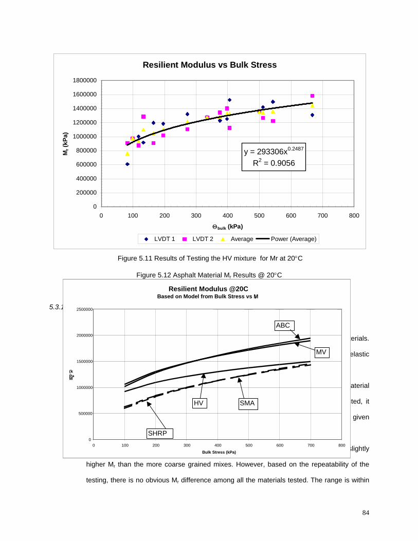
84
Resilient Modulus vs Bulk Stress
y = 293306x0.2487
R2 = 0.9056
0
200000
400000
600000
800000
1000000
1200000
1400000
1600000
1800000
0 100 200 300 400 500 600 700 800
Θbulk (kPa)
Mr (
kPa)
LVDT 1 LVDT 2 Average Power (Average)
Figure 5.11 Results of Testing the HV mixture for Mr at 20°C
Figure 5.12 Asphalt Material M Br B Results @ 20°C
5.3.1.1 Comparisons of Bound Material Behaviors
The MBr B data of the asphalt mixtures show three trends:
(1) the asphalt mixtures show significantly higher M Br B values compared to the granular materials.
This is believed to be the result of the asphalt binder, which enhances the resilient, elastic
component measured at the selected testing temperatures.
(2) The resilient modulus increases with the bulk stress, which means that the same material
could show different properties when used in different layers. From the data collected, it
appears that as the deviator stress augments, the resilient modulus increases for a given
confining pressure.
(3) The MV material, which is the finest of all the mixes tested, consistently showed slightly
higher MBr B than the more coarse grained mixes. However, based on the repeatability of the
testing, there is no obvious MBr B difference among all the materials tested. The range is within
Resilient Modulus @20CBased on Model from Bulk Stress vs Mr
0
500000
1000000
1500000
2000000
2500000
0 100 200 300 400 500 600 700 800
Bulk Stress (kPa)
Mr
(kPa
MV
SMAHV
SHRP
ABC
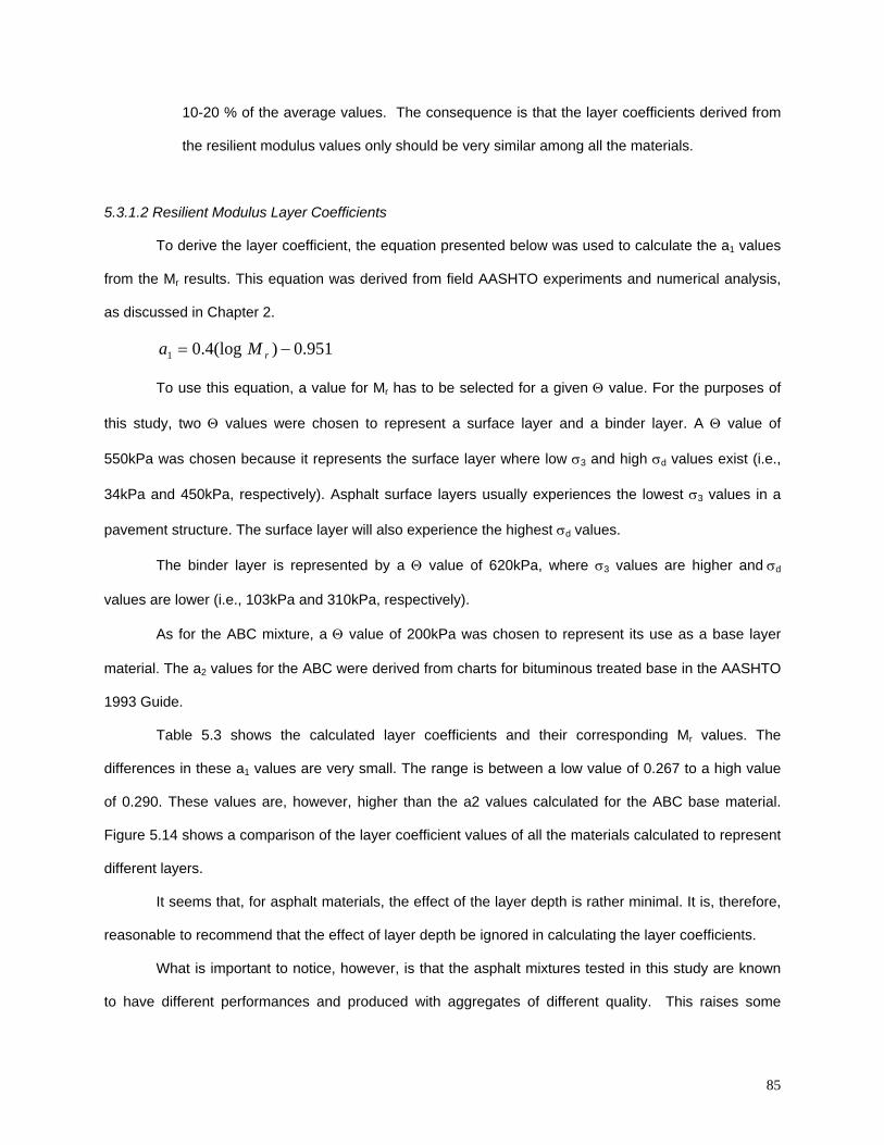
85
10-20 % of the average values. The consequence is that the layer coefficients derived from
the resilient modulus values only should be very similar among all the materials.
5.3.1.2 Resilient Modulus Layer Coefficients
To derive the layer coefficient, the equation presented below was used to calculate the a B1B values
from the MBr B results. This equation was derived from field AASHTO experiments and numerical analysis,
as discussed in Chapter 2.
951.0)(log4.01 −= rMa
To use this equation, a value for MBr B has to be selected for a given Θ value. For the purposes of
this study, two Θ values were chosen to represent a surface layer and a binder layer. A Θ value of
550kPa was chosen because it represents the surface layer where low σ B3B and high σ BdB values exist (i.e.,
34kPa and 450kPa, respectively). Asphalt surface layers usually experiences the lowest σ B3B values in a
pavement structure. The surface layer will also experience the highest σ BdB values.
The binder layer is represented by a Θ value of 620kPa, where σ B3B values are higher and σ BdB
values are lower (i.e., 103kPa and 310kPa, respectively).
As for the ABC mixture, a Θ value of 200kPa was chosen to represent its use as a base layer
material. The a B2B values for the ABC were derived from charts for bituminous treated base in the AASHTO
1993 Guide.
Table 5.3 shows the calculated layer coefficients and their corresponding MBr B values. The
differences in these a B1B values are very small. The range is between a low value of 0.267 to a high value
of 0.290. These values are, however, higher than the a2 values calculated for the ABC base material.
Figure 5.14 shows a comparison of the layer coefficient values of all the materials calculated to represent
different layers.
It seems that, for asphalt materials, the effect of the layer depth is rather minimal. It is, therefore,
reasonable to recommend that the effect of layer depth be ignored in calculating the layer coefficients.
What is important to notice, however, is that the asphalt mixtures tested in this study are known
to have different performances and produced with aggregates of different quality. This raises some
86
concerns about relying on the Mr values to estimate material contribution to performance. This concern
can be considered well founded because the resilient modulus is designed to measure only the elastic-
recoverable component. Asphalt mixtures are known to be visco-elasto-plastic in behavior and to exhibit
significant non-elastic behavior. This known fact leads to the belief that a consideration of other
properties that are non-elastic is necessary to reflect the known differences in the materials used. The
next section covers the analysis of the rutting data, which considers the combined effect of viscosity and
plasticity of asphalt mixtures.
Table 5.3 Asphalt Mixture a Bi B and M Br B Values
BulkStress Mr a1 Mr a1 Mr a1 Mr a1 Mr a2
(kPa) (MPa) (MPa) (MPa) (MPa) (MPa)550 1153 0.274 1168 0.276 1240 0.286 1111 0.267 903* 0.17*620 1195 0.28 1195 0.28 1270 0.29 1141 0.272 1077** 0.20*
*A bulk stress of 200kPa was used to reqresent the top of the base layer** A bulk stress of 380 was used to represent the mid to lower portion of the base layer
ABC20°C
SHRP SMA MV HV20°C 20°C 20°C 20°C
Figure 5.13 Layer Coefficients of Asphalt Mixtures Estimated for 2 Depths to Represent a Surface and a
Binder Layer
5.3.2 Permanent Deformation Results for Asphalt Mixtures
The data for the permanent deformation of asphalt mixtures are presented in this section They
are sorted according to material type and test conditions (σ B3B, σ BdB, temperature). Figure 5.14 shows an
example of the results for the SHRP mixture under different test conditions. The plots show the εBpB
accumulated in the specimen as a function of the load repetition (N). The designations used include three
numbers, with the first referring to confining pressure, the second to the deviator stress, and the third to
Layer Coefficients
0
0.05
0.1
0.15
0.2
0.25
0.3
0.35
0.4
SHRP SMA HV MV ABC
Binder Layer ConditionsSurface Layer Conditions
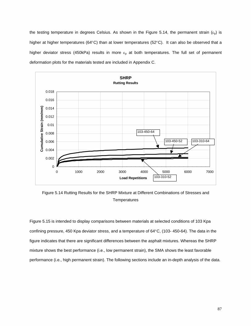
87
the testing temperature in degrees Celsius. As shown in the Figure 5.14, the permanent strain (εBpB) is
higher at higher temperatures (64°C) than at lower temperatures (52°C). It can also be observed that a
higher deviator stress (450kPa) results in more εBpB at both temperatures. The full set of permanent
deformation plots for the materials tested are included in Appendix C.
SHRPRutting Results
0
0.002
0.004
0.006
0.008
0.01
0.012
0.014
0.016
0.018
0 1000 2000 3000 4000 5000 6000 7000
Load Repetitions
Cum
ulat
ive
Stra
in (m
m/m
m)
103-450-52
103-450-64
103-310-64
103-310-52
Figure 5.14 Rutting Results for the SHRP Mixture at Different Combinations of Stresses and
Temperatures
Figure 5.15 is intended to display comparisons between materials at selected conditions of 103 Kpa
confining pressure, 450 Kpa deviator stress, and a temperature of 64°C, (103- 450-64). The data in the
figure indicates that there are significant differences between the asphalt mixtures. Whereas the SHRP
mixture shows the best performance (i.e., low permanent strain), the SMA shows the least favorable
performance (i.e., high permanent strain). The following sections include an in-depth analysis of the data.
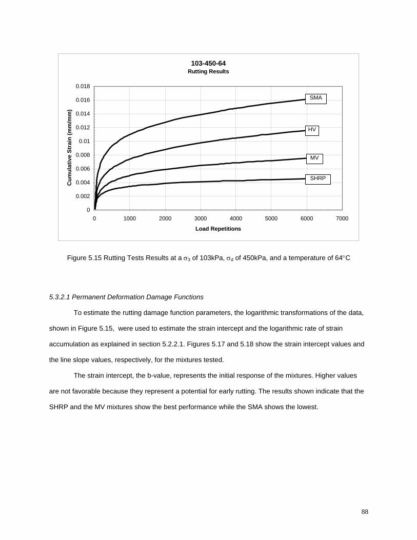
88
103-450-64Rutting Results
0
0.002
0.004
0.006
0.008
0.01
0.012
0.014
0.016
0.018
0 1000 2000 3000 4000 5000 6000 7000
Load Repetitions
Cum
ulat
ive
Stra
in (m
m/m
m)
SMA
MV
HV
SHRP
Figure 5.15 Rutting Tests Results at a σ B3B of 103kPa, σ BdB of 450kPa, and a temperature of 64°C
5.3.2.1 Permanent Deformation Damage Functions
To estimate the rutting damage function parameters, the logarithmic transformations of the data,
shown in Figure 5.15, were used to estimate the strain intercept and the logarithmic rate of strain
accumulation as explained in section 5.2.2.1. Figures 5.17 and 5.18 show the strain intercept values and
the line slope values, respectively, for the mixtures tested.
The strain intercept, the b-value, represents the initial response of the mixtures. Higher values
are not favorable because they represent a potential for early rutting. The results shown indicate that the
SHRP and the MV mixtures show the best performance while the SMA shows the lowest.
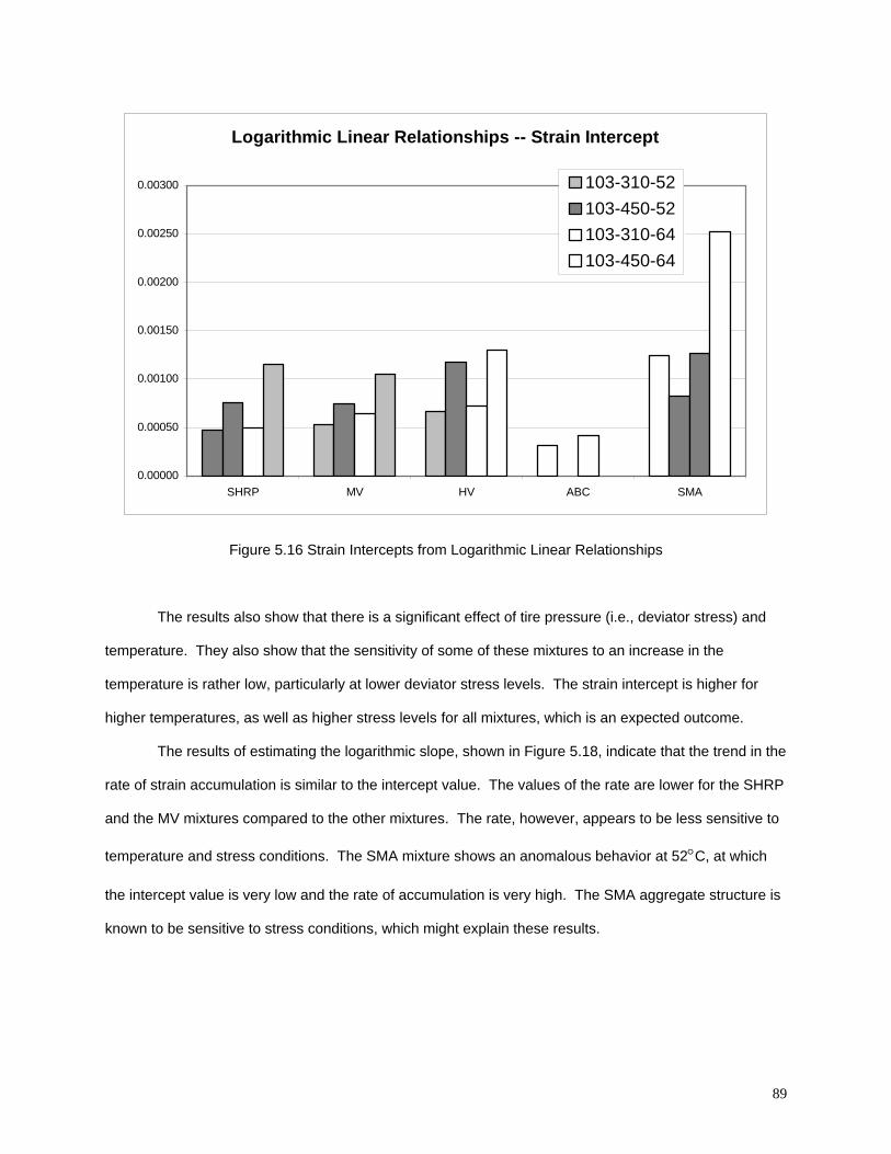
89
Logarithmic Linear Relationships -- Strain Intercept
0.00000
0.00050
0.00100
0.00150
0.00200
0.00250
0.00300
SHRP MV HV ABC SMA
103-310-52103-450-52103-310-64103-450-64
Figure 5.16 Strain Intercepts from Logarithmic Linear Relationships
The results also show that there is a significant effect of tire pressure (i.e., deviator stress) and
temperature. They also show that the sensitivity of some of these mixtures to an increase in the
temperature is rather low, particularly at lower deviator stress levels. The strain intercept is higher for
higher temperatures, as well as higher stress levels for all mixtures, which is an expected outcome.
The results of estimating the logarithmic slope, shown in Figure 5.18, indicate that the trend in the
rate of strain accumulation is similar to the intercept value. The values of the rate are lower for the SHRP
and the MV mixtures compared to the other mixtures. The rate, however, appears to be less sensitive to
temperature and stress conditions. The SMA mixture shows an anomalous behavior at 52°C, at which
the intercept value is very low and the rate of accumulation is very high. The SMA aggregate structure is
known to be sensitive to stress conditions, which might explain these results.
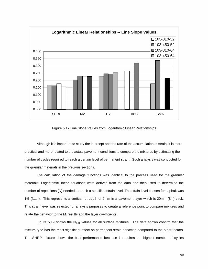
Logarithmic Linear Relationships -- Line Slope Values
0.000
0.050
0.100
0.150
0.200
0.250
0.300
0.350
0.400
SHRP MV HV ABC SMA
103-310-52103-450-52103-310-64103-450-64
Figure 5.17 Line Slope Values from Logarithmic Linear Relationships
Although it is important to study the intercept and the rate of the accumulation of strain, it is more
practical and more related to the actual pavement conditions to compare the mixtures by estimating the
number of cycles required to reach a certain level of permanent strain. Such analysis was conducted for
the granular materials in the previous sections.
The calculation of the damage functions was identical to the process used for the granular
materials. Logarithmic linear equations were derived from the data and then used to determine the
number of repetitions (N) needed to reach a specified strain level. The strain level chosen for asphalt was
1% (N0.01). This represents a vertical rut depth of 2mm in a pavement layer which is 20mm (8in) thick.
This strain level was selected for analysis purposes to create a reference point to compare mixtures and
relate the behavior to the Mr results and the layer coefficients.
Figure 5.19 shows the N0.01 values for all surface mixtures. The data shown confirm that the
mixture type has the most significant effect on permanent strain behavior, compared to the other factors.
The SHRP mixture shows the best performance because it requires the highest number of cycles
90
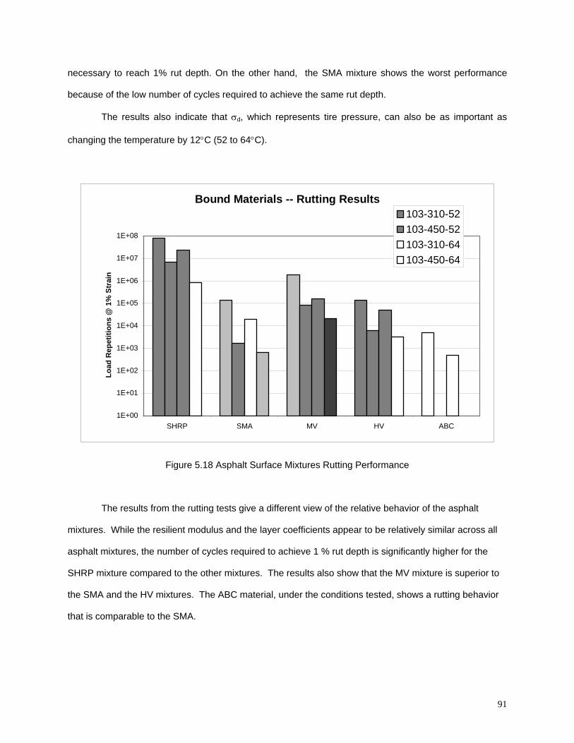
91
necessary to reach 1% rut depth. On the other hand, the SMA mixture shows the worst performance
because of the low number of cycles required to achieve the same rut depth.
The results also indicate that σ BdB, which represents tire pressure, can also be as important as
changing the temperature by 12°C (52 to 64°C).
Bound Materials -- Rutting Results
1E+00
1E+01
1E+02
1E+03
1E+04
1E+05
1E+06
1E+07
1E+08
SHRP SMA MV HV ABC
Load
Rep
etiti
ons
@ 1
% S
trai
n
103-310-52103-450-52103-310-64103-450-64
Figure 5.18 Asphalt Surface Mixtures Rutting Performance
The results from the rutting tests give a different view of the relative behavior of the asphalt
mixtures. While the resilient modulus and the layer coefficients appear to be relatively similar across all
asphalt mixtures, the number of cycles required to achieve 1 % rut depth is significantly higher for the
SHRP mixture compared to the other mixtures. The results also show that the MV mixture is superior to
the SMA and the HV mixtures. The ABC material, under the conditions tested, shows a rutting behavior
that is comparable to the SMA.
92
Some of the results collected for rutting show the kind of superior performance expected in the
case of high quality mixtures, such as the SHRP mixture. Other results, such as the comparison between
the SMA and the ABC, however, deserve further analysis to confirm the un-expected trend observed.
The SMA is expected to perform significantly better than the other mixtures tested in this
program. Without the knowledge of the performance of this specific SMA mixture in the field, it is very
difficult to determine whether or not these results reflect the actual relative performance of these
mixtures.
5.3.2.2 Temperature and Principle Stress Effects
The first noticeable trend that is observed from this data is that a higher temperature caused
more permanent deformation for the same σ B1B/σ B3B ratio. The second is that the σ B1B/σ B3B seems to have a
greater impact on permanent deformation than the temperature.
The higher temperature trend is expected. Asphalt stiffness reduces significantly when
temperature is raised, which translates into lower stiffness in asphalt mixtures. This goes hand in hand
with field results, which show that rutting presents a great problem in warmer climates.
When the testing parameters were developed, it was thought that raising the temperature would
be more of a factor than increasing the applied stress. The results, however, proved otherwise; the
asphalt mixes appear to be more dependent on the σ B1B/σ B3B ratio than on the temperature in the ranges
tested. The two permanent deformation curves corresponding to the same σ B1B/σ B3B ratio are relatively close
to one another. However, there is a significant difference between the lower and higher σ B1B/σ B3B ratios. This
implies that rutting may be more dependent on loading than on temperature.
The differences between the materials becomes greater as the σ B1B/σ B3B ratio and temperature
increase. Distinct and significant differences can be seen between the different mixes, especially at the
σ B1B/σ B3B ratio of 4.
5.3.2.3 Layer Coefficients and Permanent Deformation Comparisons
Table 5.4 shows the layer coefficients derived by the resilient modulus at 20ºC. The SHRP
mixture was not associated with the highest a B1B value. The MV mixture showed the best results; there are
only minor differences among the layer coefficients of these materials.
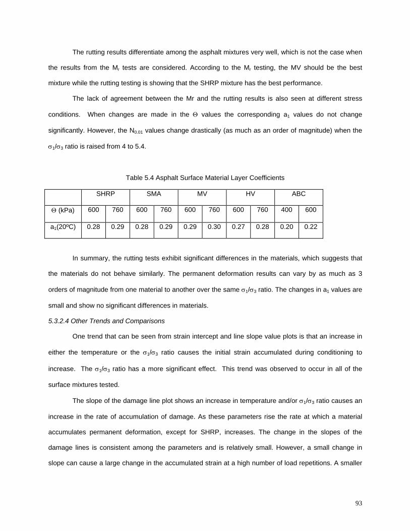
93
The rutting results differentiate among the asphalt mixtures very well, which is not the case when
the results from the MBr B tests are considered. According to the MBr B testing, the MV should be the best
mixture while the rutting testing is showing that the SHRP mixture has the best performance.
The lack of agreement between the Mr and the rutting results is also seen at different stress
conditions. When changes are made in the Θ values the corresponding a B1B values do not change
significantly. However, the N B0.01B values change drastically (as much as an order of magnitude) when the
σ B1B/σ B3B ratio is raised from 4 to 5.4.
Table 5.4 Asphalt Surface Material Layer Coefficients
SHRP SMA MV HV ABC
Θ (kPa) 600 760 600 760 600 760 600 760 400 600
a B1B(20ºC) 0.28 0.29 0.28 0.29 0.29 0.30 0.27 0.28 0.20 0.22
In summary, the rutting tests exhibit significant differences in the materials, which suggests that
the materials do not behave similarly. The permanent deformation results can vary by as much as 3
orders of magnitude from one material to another over the same σ B1B/σ B3B ratio. The changes in aB1B values are
small and show no significant differences in materials.
5.3.2.4 Other Trends and Comparisons
One trend that can be seen from strain intercept and line slope value plots is that an increase in
either the temperature or the σ B1B/σ B3B ratio causes the initial strain accumulated during conditioning to
increase. The σ B1B/σ B3B ratio has a more significant effect. This trend was observed to occur in all of the
surface mixtures tested.
The slope of the damage line plot shows an increase in temperature and/or σB1B/σ B3B ratio causes an
increase in the rate of accumulation of damage. As these parameters rise the rate at which a material
accumulates permanent deformation, except for SHRP, increases. The change in the slopes of the
damage lines is consistent among the parameters and is relatively small. However, a small change in
slope can cause a large change in the accumulated strain at a high number of load repetitions. A smaller
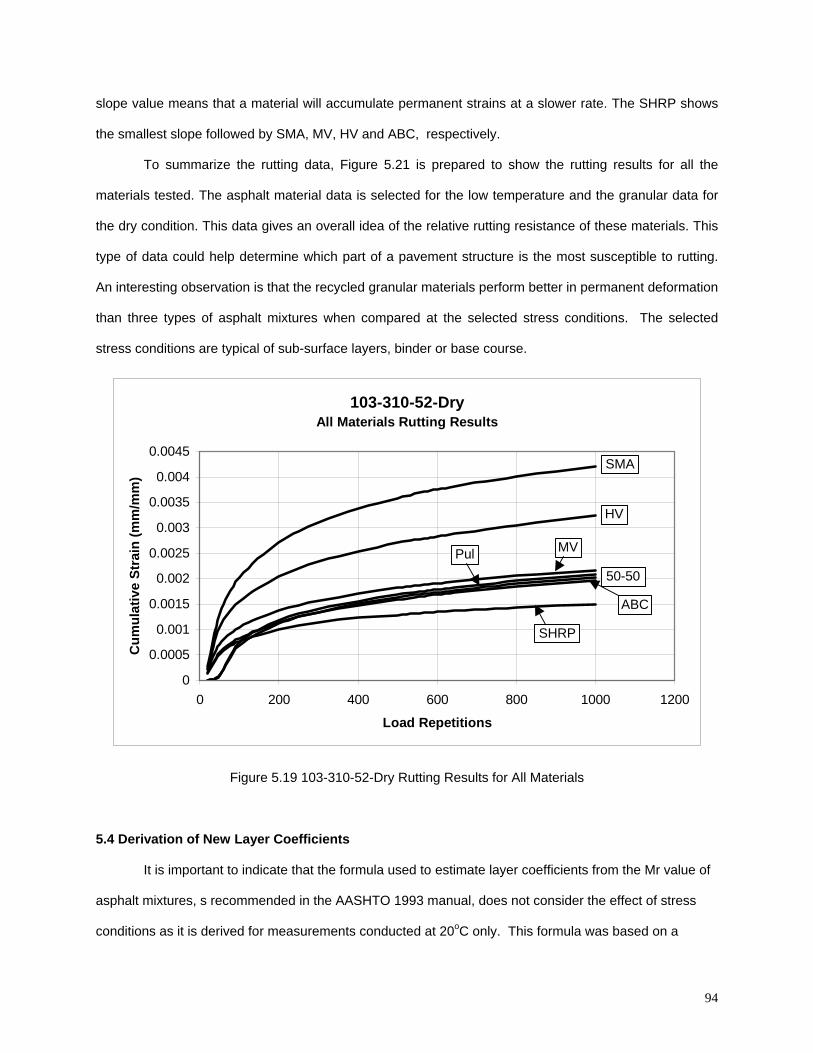
slope value means that a material will accumulate permanent strains at a slower rate. The SHRP shows
the smallest slope followed by SMA, MV, HV and ABC, respectively.
To summarize the rutting data, Figure 5.21 is prepared to show the rutting results for all the
materials tested. The asphalt material data is selected for the low temperature and the granular data for
the dry condition. This data gives an overall idea of the relative rutting resistance of these materials. This
type of data could help determine which part of a pavement structure is the most susceptible to rutting.
An interesting observation is that the recycled granular materials perform better in permanent deformation
than three types of asphalt mixtures when compared at the selected stress conditions. The selected
stress conditions are typical of sub-surface layers, binder or base course.
103-310-52-DryAll Materials Rutting Results
0
0.0005
0.001
0.0015
0.002
0.0025
0.003
0.0035
0.004
0.0045
0 200 400 600 800 1000 1200
Load Repetitions
Cum
ulat
ive
Stra
in (m
m/m
m)
SMA
HV
MVPul50-50
ABC
SHRP
Figure 5.19 103-310-52-Dry Rutting Results for All Materials
5.4 Derivation of New Layer Coefficients
It is important to indicate that the formula used to estimate layer coefficients from the Mr value of
asphalt mixtures, s recommended in the AASHTO 1993 manual, does not consider the effect of stress
conditions as it is derived for measurements conducted at 20oC only. This formula was based on a
94
95
comparative analysis of a single surface asphalt mixture that was used in the AASHTO experiment that
started in 1958. It is, therefore, necessary to proceed with extreme caution when using the Mr values to
derive the layer coefficients for newer materials.
Many State highway agencies have recognized this problem and used a layer coefficient of 0.44
for the best asphalt mixtures as a reference for their materials. Based on the research conducted in this
study, there appears to be minor differences in Mr values among asphalt mixtures. There also appears to
be major concerns regarding the reliance on the Mr values to derive new layer coefficients because of the
lack of a relationship with other performance measures, such as the rutting test results.
The only approach that could be offered to mitigate this problem is to derive layer coefficients
based on a collection of factors that affect pavement performance. These factors include resilient
modulus, damage functions, stress and temperature variations, and type of pavement structure.
For an asphalt layer, this would entail testing the resilient modulus at 20°C and 64°C, determining
rutting behavior at 64°C (# of cycles to 1% strain), and determining fatigue behavior at a temperature of
20°C (# of cycles to a 50% loss in stiffness). The layer coefficient will be based on a combination of
adjustment factors that give an equal contribution to each of the factors.
The layer coefficients would be determined by using the following general equation:
CFatigueCRuttingCR NCNBMAa ooo 2064201 ∫+∫+∫∝ (50)
where
A = resilient modulus adjustment factor
B = rutting resistance adjustment factor
C = fatigue resistance adjustment factor
N BRutting B = # of load repetitions to 1% strain
N BFatigue B = # of load repetitions to 50% loss in stiffness.
The adjustment factors could be derived by correlating the resilient modulus and damage testing
results of an asphalt surface mix to the layer coefficient of a reference material. These factors will adjust
the layer coefficient based on how a particular mixture performs in comparison to the reference material.
96
The resilient modulus adjustment factor would be a ratio of the resilient modulus of the reference material
and the resilient modulus of the mixture that is being investigated.
The rutting resistance adjustment factor is derived by using the following equation:
R
RRR
ddaSNSNB +−
= 1 (51)
where
SN BR B = The rutting structural number of the reference material
SN B1B = The rutting structural number of the tested material
a BR B = The layer coefficient of the reference material
d BR B = The layer thickness of the reference material
SN BR B is determined by using the number of cycles needed to reach 1 % permanent strain, measured from
testing the reference material, as the number of ESAL’s. Using the AASHTO design nomograph for
flexible pavements, the required structural number for these ESAL’s is determined using an assumed
pavement structure and roadbed characteristics. After taking the rutting results for the new material and
the same pavement structure, the same procedure is used to determine SN B1B.
The fatigue resistance adjustment factors could be found in a manner similar to the one just
described. However, the number of cycles to failure should be measured or estimated using the models
proposed in the literature. Since the fatigue testing is extremely time consuming and requires special
samples, it is recommended that the number of cycles-to-failure be determined using an existing model.
One of the widely used model is published by the Asphalt Institute (AI, 1982) expressed by the following
equation:
( ) 854.0291.30796.0 −−= Rtf MN ε (52)
where
N BfB = number of repetitions to fatigue failure
εBtB = strain of asphalt mixture at the bottom of the surface layer.
97
The stain at the bottom of the layer can be determined by one of the existing multi-layer elastic
analysis systems, such as the KENLAYER pavement analysis software package. It can also be assumed
based on the pavement structure being designed.
The N Bf Bof the reference material is found by taking the εBtB and MBr B and using the equation above.
The calculated number is assumed to represent the EASLs in a pavement design. The EASLs are used
in the AASHTO flexible nomograph to determine a structural number for the reference material. To find
the N BfB of a particular asphalt mixture, its measured resilient modulus is used to determine its Nf and its
structural number value. The following equation could be used to generate the fatigue resistance
adjustment factor.
R
RRF
ddaSNSNC +−
= 2 (53)
where
SN BF B = The fatigue structural number of the reference material
SN B2B = The fatigue structural number of the tested material
a BR B = The layer coefficient of the reference material
d BR B = The layer thickness of the reference material
For the granular unbound materials, the layer coefficients could be found by using a slightly
different equation:
CRuttingWetRDryR NCMBMAa o202 ∫+∫+∫∝ (54)
The equation includes the effect of moisture conditions by using the wet and dry resilient
modulus, as well as the number of cycles to failure in rutting measured, at 20 P
oPC. This approach to
determining the layer coefficient of the unbound base material utilizes current resilient modulus methods;
however, it also takes into account the material’s property of weakening when moisture contents are

increased. In addition, it includes a factor for rutting failure criterion. The unbound adjustment factors can
be found by following the processes described above.
The procedure described in the last few paragraphs includes using the inherent advantages of
the current resilient modulus tests. It also includes the failure criterion of rutting and fatigue. Another
advantage of this method is that it allows us to use the current methodologies of design, as well as
include some mechanistic analysis approach. The additional testing required to complete this method of
assigning layer coefficients includes the rutting testing which can be conducted using the same specimen
and testing set-up. It is relatively simple and has been successfully completed in this, as well as other
research.
98
99
CHAPTER SIX
FINDINGS AND FUTURE RECOMMENDATIONS
6.1 Summary of Findings
Based on the analysis of the results collected in this project, we summarize our findings below
according to area of research or group of materials tested.
Laboratory VS Field Measurements
The resilient modulus values measured in the laboratory for samples recovered from the field
could be successfully related to the values estimated from the non-destructive testing of pavements in the
field. The values estimated from field measurements are sensitive to the back calculation procedure and
the assumptions made in the analysis. It is, therefore, more realistic to measure resilient modulus in the
laboratory under different stress and temperature conditions.
Results of Unbound Reprocessed Materials
The resilient modulus values of the 50-50 mixture (i.e., 50% recycled asphalt mixture mixed with
50% virgin aggregates) and the pulverized material vary within a narrow range depending on stress and
moisture conditions. Both these materials are found to have a lower resilient modulus than the PCC-AC
recycled mixtures. Based on the results collected in comparison with the AASHTO layer coefficient
equations, the following layer coefficients are recommended for the interim use:
• 50Pcc-50Ac – 0.23
• 70Pcc-30Ac – 0.21
• 90Pcc-10Ac – 0.21
• 50-50 Milled – 0.17
• Pulverized – 0.18
These layer coefficients should be used with caution because in this study it has been found that the
rutting performance measured in the laboratory does not rank these materials in the same order as
indicated by the layer coefficients. It is believed that the current method of estimating layer coefficients is
biased toward resilience behavior. A conceptual method is presented for future consideration.
Results of Asphalt Mixtures
The resilient modulus values of the asphalt mixtures at 20oC vary within a narrow range. The
values are not highly sensitive to stress conditions but are sensitive to temperature. The rutting results of
the asphalt mixtures show very important differences between the materials; the SHRP mixture showed
the highest resistance to rutting, whereas the SMA mixture showed the least resistance to rutting. Based
on the procedure for estimating the layer coefficient values recommended by AASHTO, the asphalt
mixtures range in their layer coefficients between 0.26 and 0.30 depending on material type and stress
conditions. It is unrealistic to recommend using these values because of the significant differences in
rutting performance observed in the laboratory and the possible effect of temperature or age that is not
considered in the AASHTO procedure. It is important that the Wisconsin DOT establishes a reference
material with a reference layer coefficient. Deriving a realistic list of layer coefficients could be done only
on the basis of a comparison with this reference material. If the HV mixture tested in this project was
considered as the reference material with a layer coefficient of 0.44, the layer coefficients of the other
materials should not be any different because of the similarities in the resilient modulus values that have
been measured.
The layer coefficient of the asphalt base course is estimated at approximately 70 % of the values
for the surface layer materials. In other words, if the HV mixture is considered at 0.44, the asphaltic base
course should be at 0.31. If the actual values of Mr are used, the base material should be considered at
0.18.
A conceptual procedure is offered in this study to account for rutting and fatigue damage in deriving
a layer coefficient. The procedure requires testing mixtures for rutting, as well as the measuring resilient
modulus. The procedure could not be verified in this project and more work is required before its
implementation.
100

101
6.2 Conclusions and Recommendations
The present AASHTO method of determining layer coefficients is based on using resilient
modulus measured values to estimate the layer coefficients using specific empirical relationships. This
method can be used to consider material properties under different traffic loads, confining pressure and
deviator stress. Based on the methodology recommended by the AASHTO, the following layer
coefficients are recommended for the interim use.
• 50Pcc-50Ac – 0.23
• 70Pcc-30Ac – 0.21
• 90Pcc-10Ac – 0.21
• 50-50 Milled – 0.17
• Pulverized – 0.18
It should be mentioned however, that the research team believes that the AASHTO methodology
largely ignores other relevant factors, such as temperature sensitivity, air void, layer thickness, rutting
behavior, fatigue behavior, and age effects.
Because of this problem, it is concluded that the layer coefficients derived from resilient modulus
values should be used with certain caveats. A method is proposed that can combine resilient modulus
values with other damage factors to derive the layer coefficients. It is recommended that this method be
further explored and verified. This will require further testing and selection of reference materials that
would allow for an accurate estimation of layer coefficients.
REFERENCES
The Asphalt Institute, 1982. “Research and Development of The Asphalt Institute’s Thickness Design Manual (MS-1), (9th ed.). Research Report 82-2. Asphalt Institute.
ASTM, 1989. Nondestructive Testing of Pavements and Backcalculation of Moduli . First Volume”, ASTM
STP 1026. Harold, L. et al. (Eds.) : Philadelphia. ASTM, 1994. Nondestructive Testing of Pavements and Backcalculation of Moduli. Second Volume”,
ASTM STP 1198, Harold, L. et al, (Eds.) : Philadelphia. Brown, E. R., Haddock, J. E., Mallick, R. B., & Lynn, Y. A., 1997. “Development of a Mixture Design
Procedure for Stone Matrix Asphalt (SMA)”, Journal of the Association of Asphalt Paving Technologists. Vol. 66, pp. 1-24.
Bosscher, P. J., Benson, C.H., & Jong, D., 1997. “Method Development for Determining the Effect of
Thermal Cycles and Moisture Conditions on Pavement Structure“. Interim Report to Wisconsin Department of Transportation
Carpenter, 1990. “Layer Coefficients for Flexible Pavements”. Report No. WI/HPR-08-90, Wisconsin
Department of Transportation.
Chen, D. H. , Zaman, M. M. , and Laguros J.G. 1995, “Characterization of Base/Sub-base Materials Under Repetitive Loading,” Journal of Testing and Evaluation, Vol. 23, N. 3, pp. 180-188.
Coree, W., 1988. “Layer Coefficients in Terms of Performance and Mixture Characteristics,” Report
Number FHWA/IN/JHRP-88/13. Indiana Department of Highways: Indiana Cowher, K., 1975. “Cumulative Damage of Asphalt Materials Under Repeated-Load Indirect Tension”.
Research Report Number 183-3. Center For Highway Research – University of Texas: Austin. Dawson, A. R., Thom N. H., & Paute J.L., 1993: Mechanical Characteristics of Unbound Granular
Materials as a Function of Condition, Flexible Pavements, A. Gomes Correia, pp 35-44 Ewing, W.M., Jordetsky, W. S., & Press, F., 1957. “Elastic Waves in Layered FHWA (1994), “Pavement
Deflection Analysis”. National Highway Institute. Report No. 13127. FHWA, 1994. “Pavement Deflection Analysis,” National Highway Institute. Report No. 13127. Fwa, T. F., Low B. H., & Tan, S. A., “Compaction of Asphalt Mixtures for Laboratory Testing: Evaluation
Based on Density Profile”. Journal of Testing and Evaluation ( JTEVA). Vol. 21, No. 5, September 1993, PP. 414-421.
Galjaard, P.J., Paute, J.L., & Dawson A. R., 1993. Comparison and Performance of Repeated Load
Triaxial Test Equipment for Unbound Granular Materials, Flexible Pavements, A. Gomes Correia, pp 7-21
George, K.P., & Asce, M., 1984. “Structural Layer Coefficient for Flexible Pavement”. Journal of
Transportation Engineering. Vol. 110 (3), pp. 251-267. George, K.P., and Uddin, Waheed., 1994, “In situ and laboratory characterization of nonlinear pavement
layer moduli,” ASTM Special Technical Publication Proceedings of the Symposium on
102
Nondestructive Testing of Pavements and Backcalculation of Moduli, Jun 1993, n 1198, (12), Atlanta. pp. 203-217.
Gomez, T., & Thompson, M., R. 1983. “Structural Coefficients and Thickness Equivalency Ratios,”
Report Number FHWA/IL/UI-202: Illinois Department of Transportation. Hall, J.R., & Woods, R.D., 1970. Vibrations of Soils and Foundations. Englewood Cliffs, Prentice-Hall:
New Jersey. Hicks, R.G., & Monismith, C. L., 1971. Factors influencing the resilient response of granular materials.
Highway Research Record No 345, pp 15-31 Horak, E., 1987. “The Use of Surface Deflection Basin Measurements in the Mechanistic Analysis of
Flexible Pavements,” Proc., Vol. 1, Sixth International Conference Structural Design of Asphalt Pavements. University of Michigan: Ann Arbor.
Hossain, M., & Habib, A. 1997. “Development of Structural Layer Coefficients of Crumb Rubber Modified
Asphalt Mixes from In-Situ Deflection Tests,” Report Number K-TRAN: KSU-96-2, Kansas Department of Transportation.
Houston, W.N., Mamlouck, M.S., & Perera R.W. (1990), “Laboratory versus Nondestructive Testing for
Pavement Design,” Journal of Transportation Engineering, ASCE. Vol. 118, No.2, pp207-222. Huang, Y.H. 1993. Pavement Analysis and Design. Prentice Hall: New Jersey. Jong, D., 1997. Freeze-Thaw Effects on Stiffness of Pavement Systems. Masters thesis, University of
Wisconsin: Madison. Jong, D., & Christensen, J. D., 1997, “Layer Coefficients for New and Reprocessed Asphaltic Mixes –
Field Testing Report”, Research Report. University of Wisconsin: Madison. Khanal, P. P., & Mamlouk, M. S., 1992 “Tensile Versus Compressive Moduli of Asphalt Concrete,”
Transportation Research Record 1492, pp. 144-150. McCollough, B.F., Van Til, C .J ., and Hicks, R.G. “Evaluation of AASHO Interim Guides for Design of
Pavement Structures“. NCHRP Report 128, 1972. Michalak, C.H., Scullion, T., 1995, “Modulus 5.0: Users Manual”. Texas Transportation Institute, The
Texas A&M University System. Nazarian, S., 1984. In Situ Determination of Elastic Moduli of soil Deposits and Pavement Systems by
Spectral-Analysis-of-Surface-Waves Method. Ph.D. Dissertation. University of Texas: Austin. Nazarian, S., & Stokoe, K., H. 1984. “Nondestructive Testing of Pavements Using Surface Waves,”
Transportation Research Record 993, TRB, National Research Council, pp. 67-79. Nazarian, S., and Stokoe, K., H. 1986. “Use of Surface Waves in Pavement Evaluation,” Transportation
Research Record 1070, TRB, National Research Council. pp 132-144. Paute J.L., Dawson A.R. & Galjaard P., J. 1993. “Recommendations for Repeated Load Triaxial Test
Equipment and Procedure for Unbound Granular Materials, Flexible Pavements”, A. Gomes Correia, pp 23-34
103
Paute J. L., Hornych P., & Benaben J., P. 1993. Repeated Load Triaxial testing of Unbound Granular Materials in the French Network of “Laboratories des Ponts et Chaussees”. Euroflex 1993, session 1, Lisbon: Portugal
Ping, W., V. , G. l., & Zhiliang, Y. 1996. “Evaluation of Pavement Bearing Characteristics Using Florida
Limerock Bearing Ration Test”. Transportation Research Record 1547, pp. 53-60.
Rada, G., & and Witczak, M., W. 1981. “Comprehensive Evaluation of Laboratory Resilient Moduli Results for Granular Material”. Transportation Research Record 810, pp. 23-33.
Rada, G., & Witczak, M., W. 1982. “Material Layer Coefficients of Unbound Granular Materials from
Resilient Modulus”. Transportation Research Record 852, pp. 15-21. Rauhut, B., Lytton, B., & Darter, M. 1984. “Pavement Damage Functions for Cost Allocation, Executive
Summary,” Report Number FHWA/RD-84/017, Federal Highway Administration. Rauhut B., & Jordahl, B. 1984. “Pavement Damage Function for Cost Allocation, Vol. 3, Flexible
Pavement Damage Functions Developed from AASHO Road Test Data,” Report Number FHWA/RD-84/020, Federal Highway Administration.
Richardson N., D. 1996. “AASHTO Layer Coefficients for Cement-Stabilized Soil Bases”. Journal of
Materials in Civil Engineering v 8 n 2, pp. 83-87 Roberts, F. L., Kandhal, P. S., Brown, E. R., Lee, D. Y., & Kennedy, T. W., 1996. “Hot Mix Asphalt
Material, Mixture Design, and Construction”, Lanham, Maryland, NAPA Education Foundation Rohde, G. T., 1994. “Determining Pavement Structural Number from FWD Testing,” Transportation
Research Record 1448, (10) pp. 61-68. Sanchez-Salinero, I., Roesset, J. M., Shao, K., Stokoe, K.H., & Rix, G.J., 1987, “Analytical Evaluation Of
Variables Affecting Surface Wave Testing of Pavements,” Transportation Research Record 1136, TRB, National Research Council. pp. 132-144.
Sebaaly, P., Tabatabaee, N., Bonaquist, R., & Anderson, D. 1989. “Evaluating Structural Damage of
Flexible Pavements Using Cracking and Falling Weight Deflectometer,” Transportation Research Record 1227, TRB, National Research Council. pp. 44-52.
SHRP 1993a. “Layer Moduli Backcalculation Precedure: Software Selection”. SHRP-P-651, Strategic
Highway Research Program, National Research Council, Washington, D.C. Sheu, J., Stokoe, K.H., Roesset, J. M., and Hudson, W.R., “Applications and Limitations of the Spectral-
Analysis-of-Surface-Waves Method,” Center for Transportation Research 437-3F, The University of Texas at Austin.
Stokoe, K.H., Lee, N.U., & Rits, M.P., 1994, “Repeated Measurements of In Situ Soil Stiffness with
Permanently Embedded Geophones,” Dynamic Geotechnical Testing II, ASTM STP 1213, Ronald et al. (Eds.), ASTM, Philadelphia.
Tan, S. A., Low, B. H., & Fwa, T., F. 1994. “Behavior of Asphalt concrete Mixtures in Triaxial
Compression,” Journal of Testing and Evaluation, JTEVA. Vol. 22, No. 3, pp. 195-203. Thomas, S., 1997. Investigation of Modified Asphalt Performance Using SHRP Binder Specification.
Masters Thesis, University of Wisconsin: Madison Uzan, J. 1992. “Resilient Characteristics of Pavement Materials “. Short Communication, International
Journal for Numerical and Analytical Methods in Geomechanics, Vol. 16, No. 6, pp. 453-459.
104

Witczak, M. W., & Uzan, J. 1988. ”The Universal Airport Pavement Design System; Report I of IV:
Granular Material Characterization”. University of Maryland, Dept. Of C. E. Wisconsin Department of Transportation, 1994. “Facilities Development Manual,” Department of
Transportation, State of Wisconsin.
105
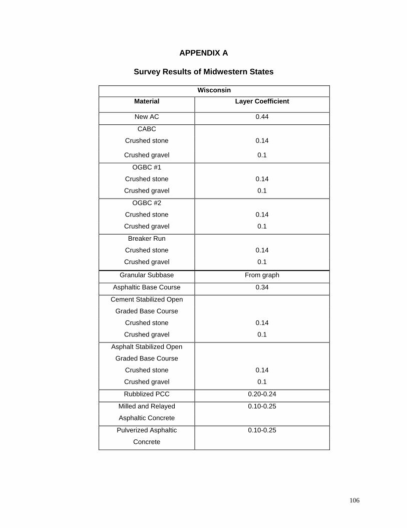
APPENDIX A
Survey Results of Midwestern States
Wisconsin Material Layer Coefficient
New AC 0.44
CABC
Crushed stone 0.14
Crushed gravel 0.1
OGBC #1
Crushed stone 0.14
Crushed gravel 0.1
OGBC #2
Crushed stone 0.14
Crushed gravel 0.1
Breaker Run
Crushed stone 0.14
Crushed gravel 0.1
Granular Subbase From graph
Asphaltic Base Course 0.34
Cement Stabilized Open
Graded Base Course
Crushed stone 0.14
Crushed gravel 0.1
Asphalt Stabilized Open
Graded Base Course
Crushed stone 0.14
Crushed gravel 0.1
Rubblized PCC 0.20-0.24
Milled and Relayed 0.10-0.25
Asphaltic Concrete
Pulverized Asphaltic 0.10-0.25
Concrete
106

Design Methods Used by Surveyed States
AASHTO DM
State Design Agency Contact Name 86 93 other
Illinois DOT David Lippert X
Indiana DOT Dave Andrewski X
Iowa DOT Chris Brakke X
Kansas DOT Rick Barezinsky X
Kentucky DOT Gary W Sharpe X
Michigan DOT Curtis Bleech X
Minnesota DOT Duane Young X X
Missouri DOT Denis Glascock X X
Nebraska DOT Dan Nichols X
North Dakota DOT Darcy Rosendahl X
Ohio DOT Aric A Morse X
South Dakota DOT Gill Hedman X
107
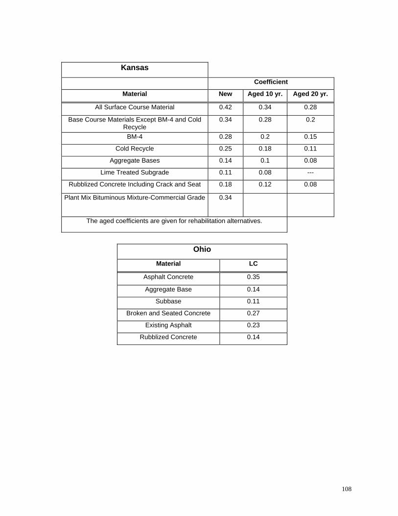
Kansas
Coefficient
Material New Aged 10 yr. Aged 20 yr.
All Surface Course Material 0.42 0.34 0.28
Base Course Materials Except BM-4 and Cold Recycle
0.34 0.28 0.2
BM-4 0.28 0.2 0.15
Cold Recycle 0.25 0.18 0.11
Aggregate Bases 0.14 0.1 0.08
Lime Treated Subgrade 0.11 0.08 ---
Rubblized Concrete Including Crack and Seat 0.18 0.12 0.08
Plant Mix Bituminous Mixture-Commercial Grade 0.34
The aged coefficients are given for rehabilitation alternatives.
Ohio
Material LC
Asphalt Concrete 0.35
Aggregate Base 0.14
Subbase 0.11
Broken and Seated Concrete 0.27
Existing Asphalt 0.23
Rubblized Concrete 0.14
108
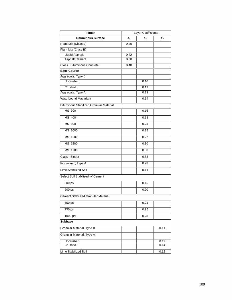
Illinois Layer Coefficients
Bituminous Surface a1 a2 a3
Road Mix (Class B) 0.20
Plant Mix (Class B)
Liquid Asphalt 0.22 Asphalt Cement 0.30
Class I Bituminous Concrete 0.40
Base Course
Aggregate, Type B Uncrushed 0.10
Crushed 0.13
Aggregate, Type A 0.13
Waterbound Macadam 0.14
Bituminous Stabilized Granular Material
MS 300 0.16
MS 400 0.18
MS 800 0.23
MS 1000 0.25
MS 1200 0.27
MS 1500 0.30
MS 1700 0.33
Class I Binder 0.33
Pozzolanic, Type A 0.28
Lime Stabilized Soil 0.11
Select Soil Stabilized w/ Cement
300 psi 0.15
500 psi 0.20
Cement Stabilized Granular Material
650 psi 0.23
750 psi 0.25
1000 psi 0.28
Subbase
Granular Material, Type B 0.11
Granular Material, Type A
Uncrushed 0.12 Crushed 0.14
Lime Stabilized Soil 0.12
109
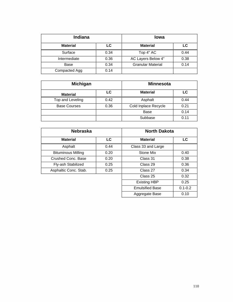
Indiana Iowa
Material LC Material LC
Surface 0.34 Top 4" AC 0.44 Intermediate 0.36 AC Layers Below 4" 0.38
Base 0.34 Granular Material 0.14 Compacted Agg 0.14
Michigan Minnesota
Material LC Material LC
Top and Leveling 0.42 Asphalt 0.44 Base Courses 0.36 Cold Inplace Recycle 0.21
Base 0.14 Subbase 0.11
Nebraska North Dakota
Material LC Material LC
Asphalt 0.44 Class 33 and Large Bituminous Milling 0.20 Stone Mix 0.40
Crushed Conc. Base 0.20 Class 31 0.38 Fly-ash Stabilized 0.25 Class 29 0.36
Asphaltic Conc. Stab. 0.25 Class 27 0.34 Class 25 0.32
Existing HBP 0.25 Emulsified Base 0.1-0.2 Aggregate Base 0.10
110
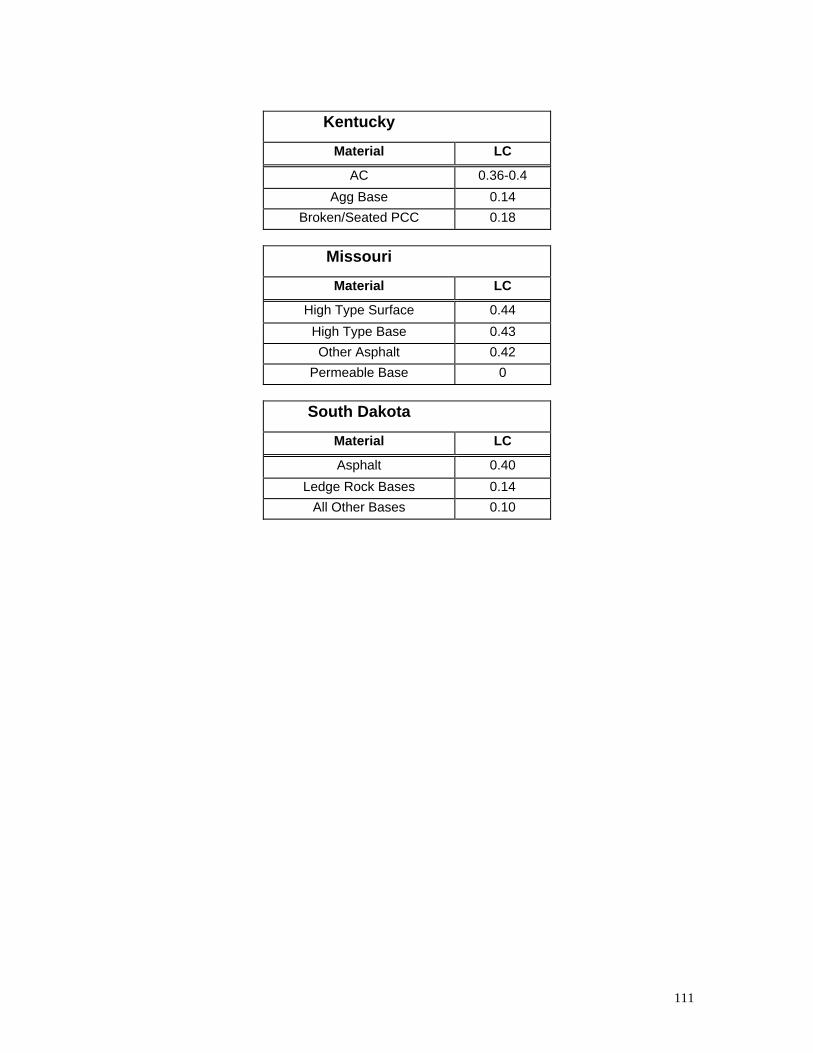
Kentucky
Material LC
AC 0.36-0.4 Agg Base 0.14
Broken/Seated PCC 0.18
Missouri
Material LC
High Type Surface 0.44 High Type Base 0.43 Other Asphalt 0.42
Permeable Base 0
South Dakota
Material LC
Asphalt 0.40 Ledge Rock Bases 0.14
All Other Bases 0.10
111
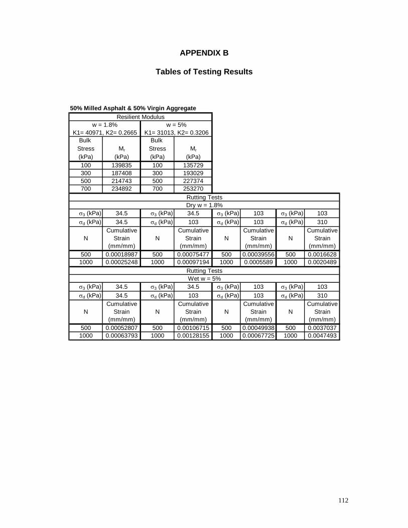
112
APPENDIX B
Tables of Testing Results
50% Milled Asphalt & 50% Virgin Aggregate
Bulk Bulk Stress Mr Stress Mr
(kPa) (kPa) (kPa) (kPa)100 139835 100 135729300 187408 300 193029500 214743 500 227374700 234892 700 253270
σ3 (kPa) 34.5 σ3 (kPa) 34.5 σ3 (kPa) 103 σ3 (kPa) 103σd (kPa) 34.5 σd (kPa) 103 σd (kPa) 103 σd (kPa) 310
Cumulative Cumulative Cumulative CumulativeN Strain N Strain N Strain N Strain
(mm/mm) (mm/mm) (mm/mm) (mm/mm)500 0.00018987 500 0.00075477 500 0.00039556 500 0.00166281000 0.00025248 1000 0.00097194 1000 0.0005589 1000 0.0020489
σ3 (kPa) 34.5 σ3 (kPa) 34.5 σ3 (kPa) 103 σ3 (kPa) 103σd (kPa) 34.5 σd (kPa) 103 σd (kPa) 103 σd (kPa) 310
Cumulative Cumulative Cumulative CumulativeN Strain N Strain N Strain N Strain
(mm/mm) (mm/mm) (mm/mm) (mm/mm)500 0.00052807 500 0.00106715 500 0.00049938 500 0.00370371000 0.00063793 1000 0.00128155 1000 0.00067725 1000 0.0047493
Resilient Modulusw = 1.8% w = 5%
K1= 40971, K2= 0.2665 K1= 31013, K2= 0.3206
Rutting TestsDry w = 1.8%
Rutting TestsWet w = 5%
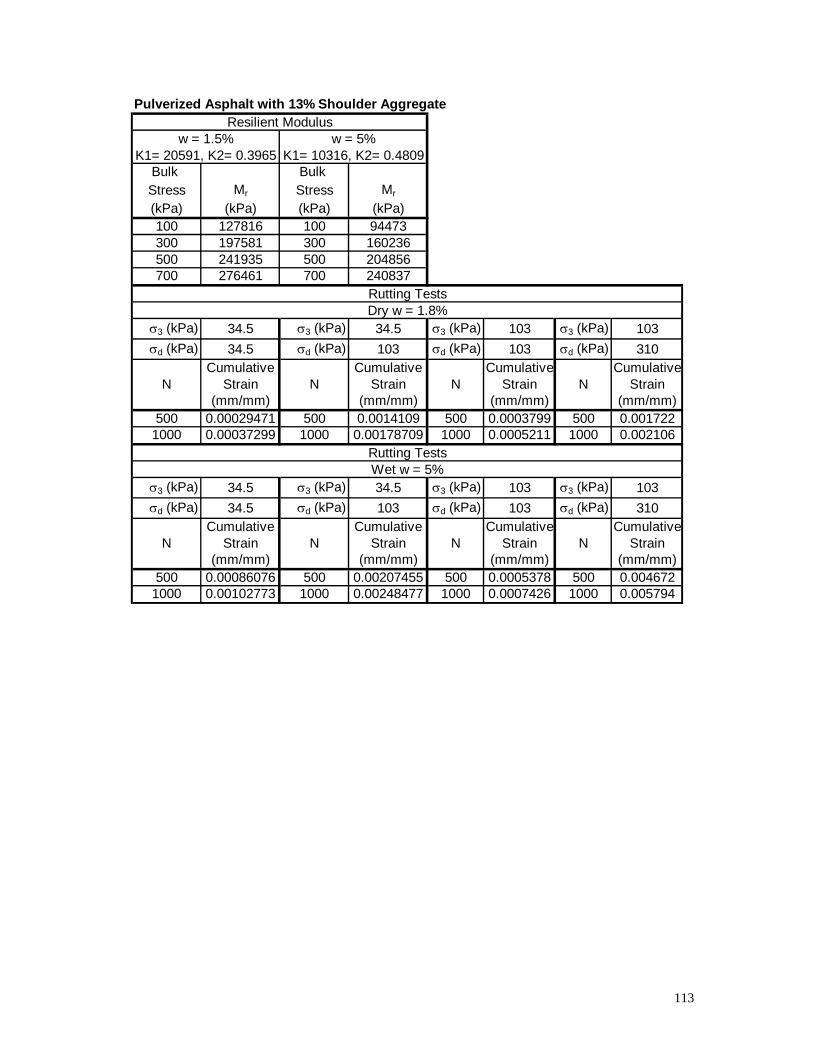
113
Pulverized Asphalt with 13% Shoulder Aggregate
Bulk Bulk Stress Mr Stress Mr
(kPa) (kPa) (kPa) (kPa)100 127816 100 94473300 197581 300 160236500 241935 500 204856700 276461 700 240837
σ3 (kPa) 34.5 σ3 (kPa) 34.5 σ3 (kPa) 103 σ3 (kPa) 103σd (kPa) 34.5 σd (kPa) 103 σd (kPa) 103 σd (kPa) 310
Cumulative Cumulative Cumulative CumulativeN Strain N Strain N Strain N Strain
(mm/mm) (mm/mm) (mm/mm) (mm/mm)500 0.00029471 500 0.0014109 500 0.0003799 500 0.001722
1000 0.00037299 1000 0.00178709 1000 0.0005211 1000 0.002106
σ3 (kPa) 34.5 σ3 (kPa) 34.5 σ3 (kPa) 103 σ3 (kPa) 103σd (kPa) 34.5 σd (kPa) 103 σd (kPa) 103 σd (kPa) 310
Cumulative Cumulative Cumulative CumulativeN Strain N Strain N Strain N Strain
(mm/mm) (mm/mm) (mm/mm) (mm/mm)500 0.00086076 500 0.00207455 500 0.0005378 500 0.004672
1000 0.00102773 1000 0.00248477 1000 0.0007426 1000 0.005794
Resilient Modulusw = 1.5% w = 5%
K1= 20591, K2= 0.3965 K1= 10316, K2= 0.4809
Rutting TestsDry w = 1.8%
Rutting TestsWet w = 5%

114
Asphalt Base Course
Bulk Bulk Stress Mr Stress Mr
(kPa) (kPa) (kPa) (kPa)100 294441.9 100 192890300 495518.3 300 329625500 631206.7 500 422878.4700 740298.9 700 498290.3
σ3 (kPa) 103 σ3 (kPa) 103 σ3 (kPa) 103 σ3 (kPa) 103σd (kPa) 103 σd (kPa) 310 σd (kPa) 103 σd (kPa) 310
Cumulative Cumulative Cumulative CumulativeN Strain N Strain N Strain N Strain
(mm/mm) (mm/mm) (mm/mm) (mm/mm)1000 0.0001142 1000 0.0019632 1000 0.0002758 1000 0.0037342500 0.0001419 2500 0.0025199 2500 0.0003616 2500 0.00501814000 0.0001512 4000 0.0028326 4000 0.0004035 4000 0.00579916000 0.0001543 6000 0.0031207 6000 0.0004491 6000 0.0065681
Rutting Tests52 C 64 C
Resilient Modulus from Power Model52 C 64 C
K1= 33220, K2= 0.4738 K1= 20414, K2= 0.4877
Stone Matrix Asphalt
Bulk Bulk Stress Mr Stress Mr
(kPa) (kPa) (kPa) (kPa)100 206189.4 100 144447.35300 319868.7 300 254431.08500 392323.8 500 331046.37700 448799.2 700 393721.02
σ3 (kPa) 103 σ3 (kPa) 103 σ3 (kPa) 103 σ3 (kPa) 103σd (kPa) 310 σd (kPa) 450 σd (kPa) 310 σd (kPa) 450
Cumulative Cumulative Cumulative CumulativeN Strain N Strain N Strain N Strain
(mm/mm) (mm/mm) (mm/mm) (mm/mm)1000 0.0042115 1000 0.008426 1000 0.0053722 1000 0.01100722500 0.0050044 2500 0.0011442 2500 0.0065471 2500 0.01341774000 0.0053799 4000 0.012445 4000 0.0071748 4000 0.0148036000 0.0057053 6000 0.015376 6000 0.007766 6000 0.0161769
Rutting Tests52 C 64 C
Resilient Modulus from Power Model52 C 64 C
K1= 46874, K2= .3042 K1= 13462, K2= 0.5153
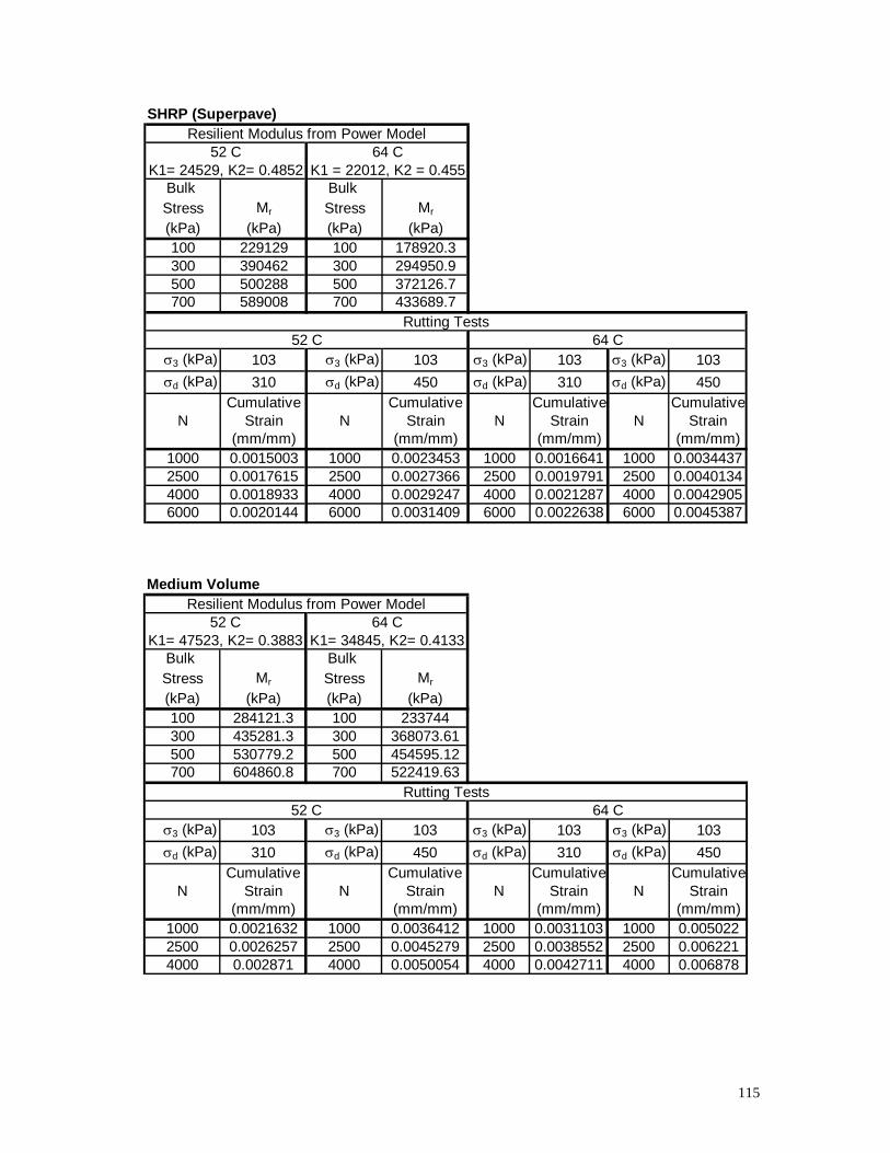
115
SHRP (Superpave)
Bulk Bulk Stress Mr Stress Mr
(kPa) (kPa) (kPa) (kPa)100 229129 100 178920.3300 390462 300 294950.9500 500288 500 372126.7700 589008 700 433689.7
σ3 (kPa) 103 σ3 (kPa) 103 σ3 (kPa) 103 σ3 (kPa) 103σd (kPa) 310 σd (kPa) 450 σd (kPa) 310 σd (kPa) 450
Cumulative Cumulative Cumulative CumulativeN Strain N Strain N Strain N Strain
(mm/mm) (mm/mm) (mm/mm) (mm/mm)1000 0.0015003 1000 0.0023453 1000 0.0016641 1000 0.00344372500 0.0017615 2500 0.0027366 2500 0.0019791 2500 0.00401344000 0.0018933 4000 0.0029247 4000 0.0021287 4000 0.00429056000 0.0020144 6000 0.0031409 6000 0.0022638 6000 0.0045387
Resilient Modulus from Power Model
Rutting Tests52 C 64 C
52 C 64 CK1= 24529, K2= 0.4852 K1 = 22012, K2 = 0.455
Medium Volume
Bulk Bulk Stress Mr Stress Mr
(kPa) (kPa) (kPa) (kPa)100 284121.3 100 233744300 435281.3 300 368073.61500 530779.2 500 454595.12700 604860.8 700 522419.63
σ3 (kPa) 103 σ3 (kPa) 103 σ3 (kPa) 103 σ3 (kPa) 103σd (kPa) 310 σd (kPa) 450 σd (kPa) 310 σd (kPa) 450
Cumulative Cumulative Cumulative CumulativeN Strain N Strain N Strain N Strain
(mm/mm) (mm/mm) (mm/mm) (mm/mm)1000 0.0021632 1000 0.0036412 1000 0.0031103 1000 0.0050222500 0.0026257 2500 0.0045279 2500 0.0038552 2500 0.0062214000 0.002871 4000 0.0050054 4000 0.0042711 4000 0.006878
Resilient Modulus from Power Model
Rutting Tests52 C 64 C
52 C 64 CK1= 47523, K2= 0.3883 K1= 34845, K2= 0.4133
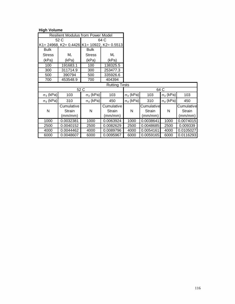
116
High Volume
Bulk Bulk Stress Mr Stress Mr
(kPa) (kPa) (kPa) (kPa)100 191683.1 100 138325.5300 311714.9 300 253477.3500 390794 500 335926.6700 453548.9 700 404394
σ3 (kPa) 103 σ3 (kPa) 103 σ3 (kPa) 103 σ3 (kPa) 103σd (kPa) 310 σd (kPa) 450 σd (kPa) 310 σd (kPa) 450
Cumulative Cumulative Cumulative CumulativeN Strain N Strain N Strain N Strain
(mm/mm) (mm/mm) (mm/mm) (mm/mm)1000 0.0032381 1000 0.0063924 1000 0.0038641 1000 0.00740152500 0.0040152 2500 0.0082629 2500 0.0048685 2500 0.0093394000 0.0044462 4000 0.0089796 4000 0.0054161 4000 0.01050276000 0.0048607 6000 0.0095967 6000 0.0059165 6000 0.0116293
Rutting Tests52 C 64 C
Resilient Modulus from Power Model52 C 64 C
K1= 24968, K2= 0.4426 K1= 10922, K2= 0.5513
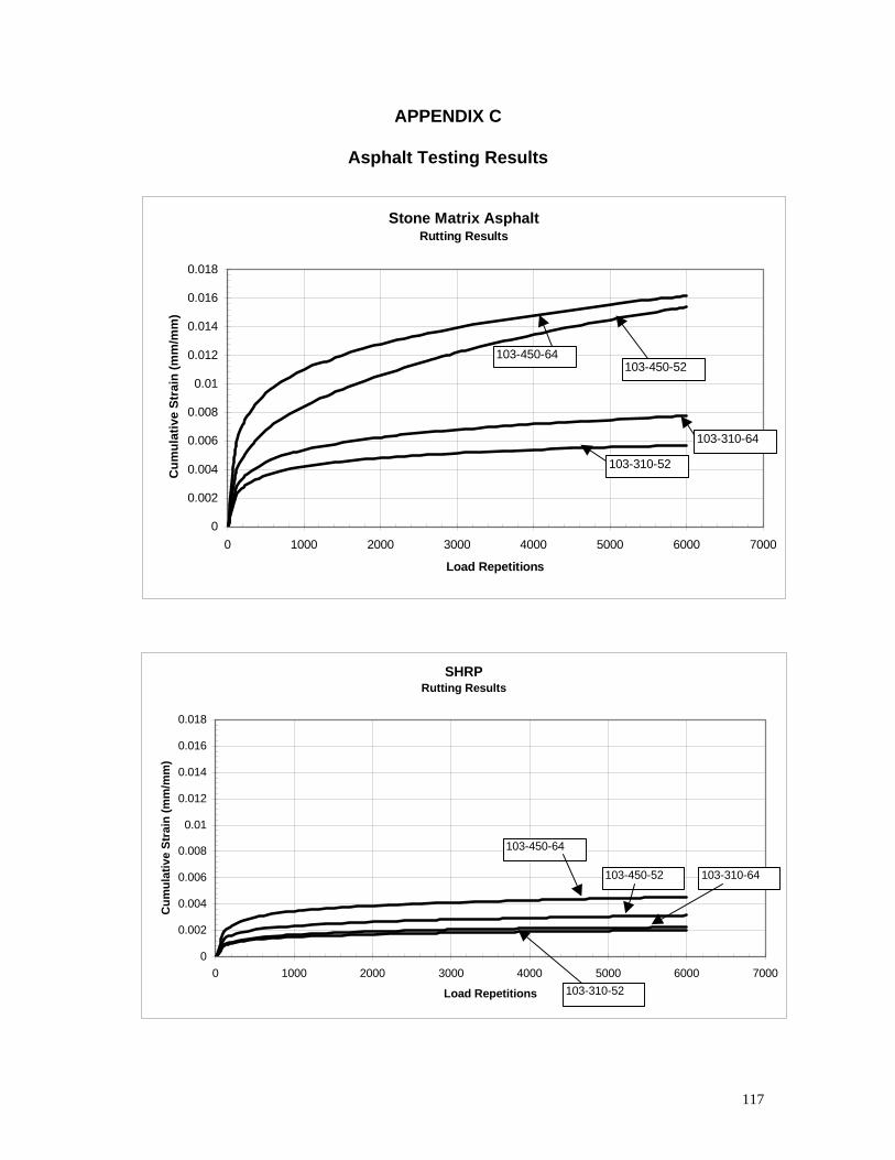
APPENDIX C
Asphalt Testing Results
Stone Matrix AsphaltRutting Results
0
0.002
0.004
0.006
0.008
0.01
0.012
0.014
0.016
0.018
0 1000 2000 3000 4000 5000 6000 7000
Load Repetitions
Cum
ulat
ive
Stra
in (m
m/m
m)
103-310-52
103-310-64
103-450-64103-450-52
SHRPRutting Results
0
0.002
0.004
0.006
0.008
0.01
0.012
0.014
0.016
0.018
0 1000 2000 3000 4000 5000 6000 7000
Load Repetitions
Cum
ulat
ive
Stra
in (m
m/m
m)
103-450-52
103-450-64
103-310-64
103-310-52
117
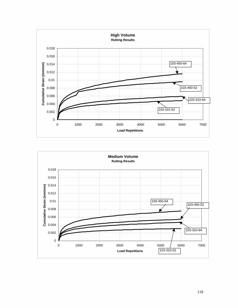
High VolumeRutting Results
0
0.002
0.004
0.006
0.008
0.01
0.012
0.014
0.016
0.018
0 1000 2000 3000 4000 5000 6000 7000
Load Repetitions
Cum
ulat
ive
Stra
in (m
m/m
m)
103-310-52
103-310-64
103-450-64
103-450-52
Medium VolumeRutting Results
0
0.002
0.004
0.006
0.008
0.01
0.012
0.014
0.016
0.018
0 1000 2000 3000 4000 5000 6000 7000
Load Repetitions
Cum
ulat
ive
Stra
in (m
m/m
m)
103-450-52103-450-64
103-310-64
103-310-52
118
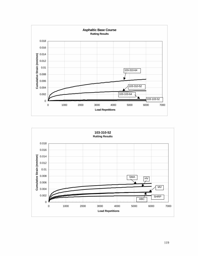
Asphaltic Base CourseRutting Results
0
0.002
0.004
0.006
0.008
0.01
0.012
0.014
0.016
0.018
0 1000 2000 3000 4000 5000 6000 7000
Load Repetitions
Cum
ulat
ive
Stra
in (m
m/m
m)
103-103-52
103-310-64
103-310-52
103-103-64
103-310-52Rutting Results
0
0.002
0.004
0.006
0.008
0.01
0.012
0.014
0.016
0.018
0 1000 2000 3000 4000 5000 6000 7000
Load Repetitions
Cum
ulat
ive
Stra
in (m
m/m
m)
SMA HV
MV
ABCSHRP
119
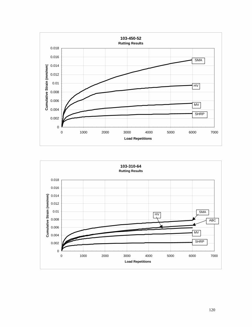
103-450-52Rutting Results
0
0.002
0.004
0.006
0.008
0.01
0.012
0.014
0.016
0.018
0 1000 2000 3000 4000 5000 6000 7000
Load Repetitions
Cum
ulat
ive
Stra
in (m
m/m
m)
SMA
MV
HV
SHRP
103-310-64Rutting Results
0
0.002
0.004
0.006
0.008
0.01
0.012
0.014
0.016
0.018
0 1000 2000 3000 4000 5000 6000 7000
Load Repetitions
Cum
ulat
ive
Stra
in (m
m/m
m)
SHRP
MV
SMAHV
ABC
120
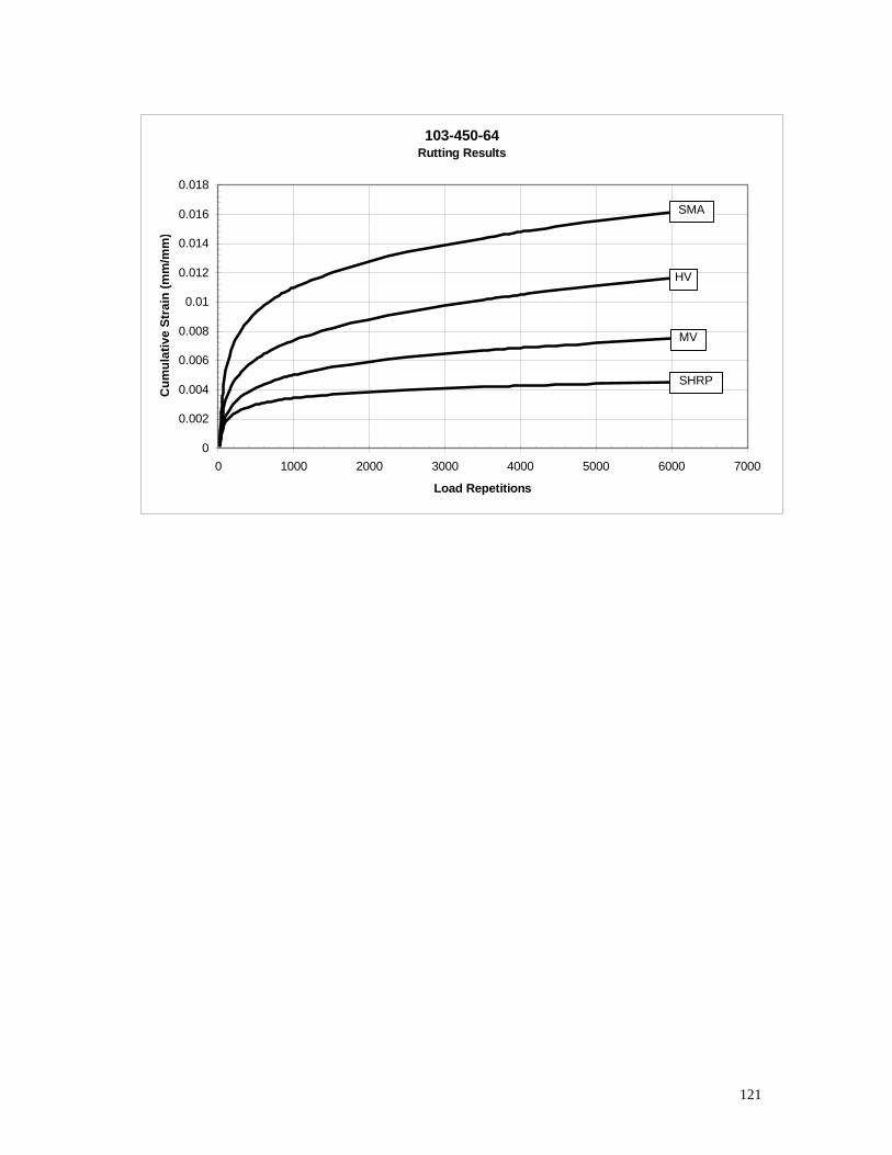
103-450-64Rutting Results
0
0.002
0.004
0.006
0.008
0.01
0.012
0.014
0.016
0.018
0 1000 2000 3000 4000 5000 6000 7000
Load Repetitions
Cum
ulat
ive
Stra
in (m
m/m
m)
SMA
MV
HV
SHRP
121
122
APPENDIX D
Teflon Compliance
With the use of 8.8in asphalt specimens, edge friction between the specimens and the
top and bottom plates became a concern. To alleviate the problem, the use of two Teflon discs
was adopted. The discs are 3.023mm in thickness; it was assumed that the deformation would be
negligible. However, this assumption proved to be incorrect.
The very first MBr B tests performed (1P
stP generation tests) gave results that were too low and
highly questionable. The values for asphalt M Br B were lower than those of the granular materials.
This directly led to the discovery of the confining pressure problem mentioned previously.
However, even after this problem was corrected, the values for asphalt MBr B seemed to be lower
than those generated by the field tests and other previous research.
Newcomb (1987) compared laboratory M Br B to field MBr B and found that they varied by 0.3 to
0.4 for asphalt mixtures. Houston et al. (1992) found that the laboratory M Br B on average were 1.5
times higher than the field MBr B values. Khanal et al. tested asphalt using the diametrical resilient
modulus method (ASTM D 4123) in harmonic compression and alternate tension and
compression. They found laboratory moduli to average 1741MPa for harmonic M Br B and 1378MPa
for alternate MBr B. Both of these came from tests at 40°C. Even though these previous studies did
not use tri-axial equipment and the tests were conducted at lower temperatures, the values
collected in this study still seemed to be on the low side.
Therefore, in the effort to determine where unwanted deformations might be coming
from, an asphalt M Br B test was conducted without the Teflon discs. This test showed a significant
difference from the tests performed with the Teflon discs in place. Compliance tests were run on
the Teflon discs. It was found that the Teflon discs were indeed deforming. The tests were
conducted by placing the discs in between rigid steel plates and running the tri-axial at various
deviator stresses. Then the discs were removed and the steel was tested solely under the same
parameters. Figure D1 shows the deformation values of the Teflon discs in tri-axial compression;
the steel deformation was subtracted out to arrive at the Teflon discs values.
123
Figure D1 shows that the deformation vs. σ BdB follows a somewhat logarithmic trend.
However, this trend was not reliable enough to be used as an adjustment for the data. Also,
some of the deformations shown for the Teflon discs were greater than those from the asphalt M Br B
tests themselves. The deformation data could not be used directly; however, it showed that there
was a problem and it needed to be explored.
In order to quantify the effect of the Teflon discs, additional M Br B tests were preformed to
see if a trend between the tests with and without the Teflon discs could be noticed. The result of
the SMA testing is shown in Figure D2. The two additional testing results for the SHRP and MV
mixtures are shown in Figures D3 & D4. The SMA and MV tests were conducted at 52°C and the
SHRP mixture test was conducted at 64°C.
These three tests show that there is a similar trend in the effect of the Teflon discs. In all
three cases the tests without the Teflon discs are approximately 100,000kPa higher at low bulk
stress (Θ) and 150,000kPa higher at high Θ values. All of the specimens were compacted from
reused material and were conducted under similar conditions. The analysis of these sets of tests
is discussed further in the next chapter.
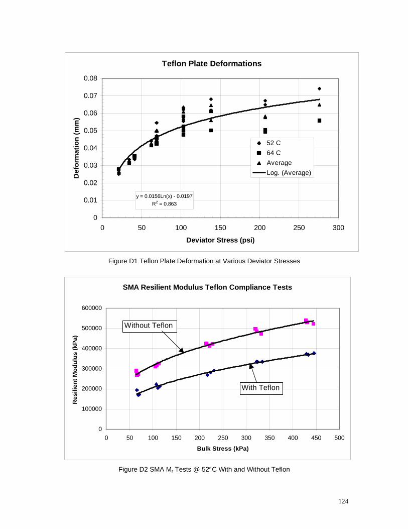
124
Teflon Plate Deformations
y = 0.0156Ln(x) - 0.0197R2 = 0.863
0
0.01
0.02
0.03
0.04
0.05
0.06
0.07
0.08
0 50 100 150 200 250 300
Deviator Stress (psi)
Def
orm
atio
n (m
m)
52 C64 CAverageLog. (Average)
Figure D1 Teflon Plate Deformation at Various Deviator Stresses
SMA Resilient Modulus Teflon Compliance Tests
0
100000
200000
300000
400000
500000
600000
0 50 100 150 200 250 300 350 400 450 500
Bulk Stress (kPa)
Res
ilien
t Mod
ulus
(kPa
)
With Teflon
Without Teflon
Figure D2 SMA M Br B Tests @ 52°C With and Without Teflon
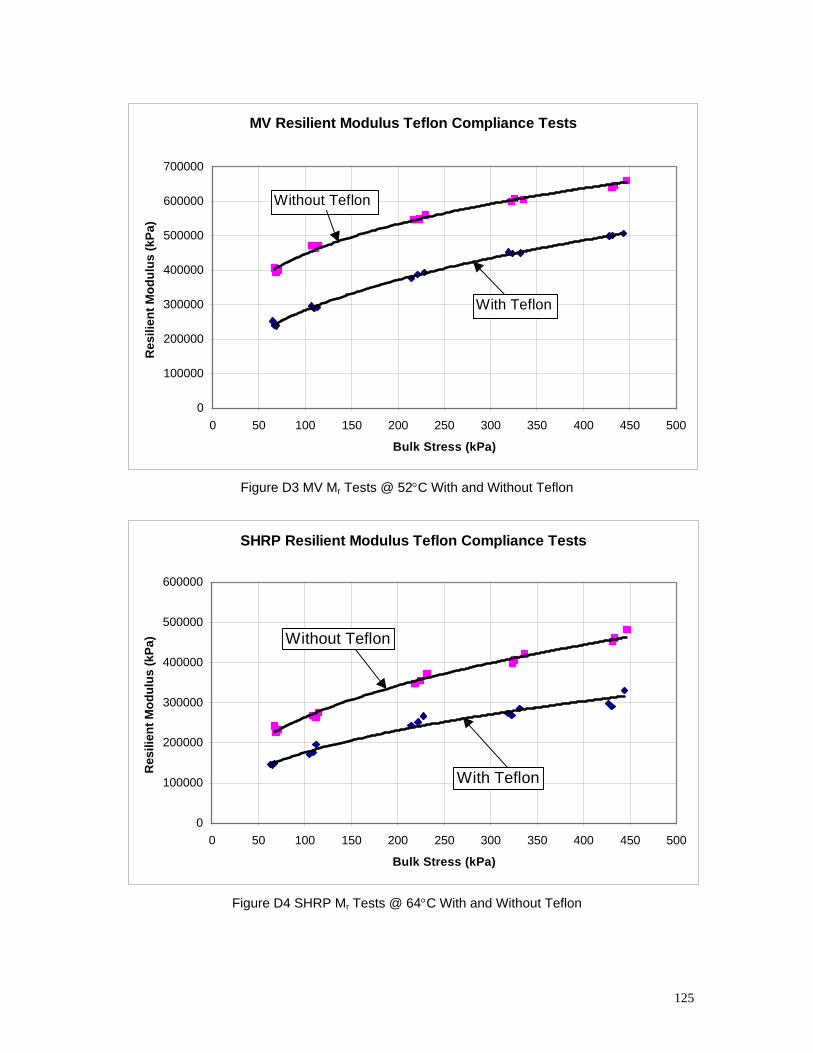
125
MV Resilient Modulus Teflon Compliance Tests
0
100000
200000
300000
400000
500000
600000
700000
0 50 100 150 200 250 300 350 400 450 500
Bulk Stress (kPa)
Res
ilien
t Mod
ulus
(kPa
)
With Teflon
Without Teflon
Figure D3 MV M Br B Tests @ 52°C With and Without Teflon
SHRP Resilient Modulus Teflon Compliance Tests
0
100000
200000
300000
400000
500000
600000
0 50 100 150 200 250 300 350 400 450 500
Bulk Stress (kPa)
Res
ilien
t Mod
ulus
(kPa
)
With Teflon
Without Teflon
Figure D4 SHRP M Br B Tests @ 64°C With and Without Teflon
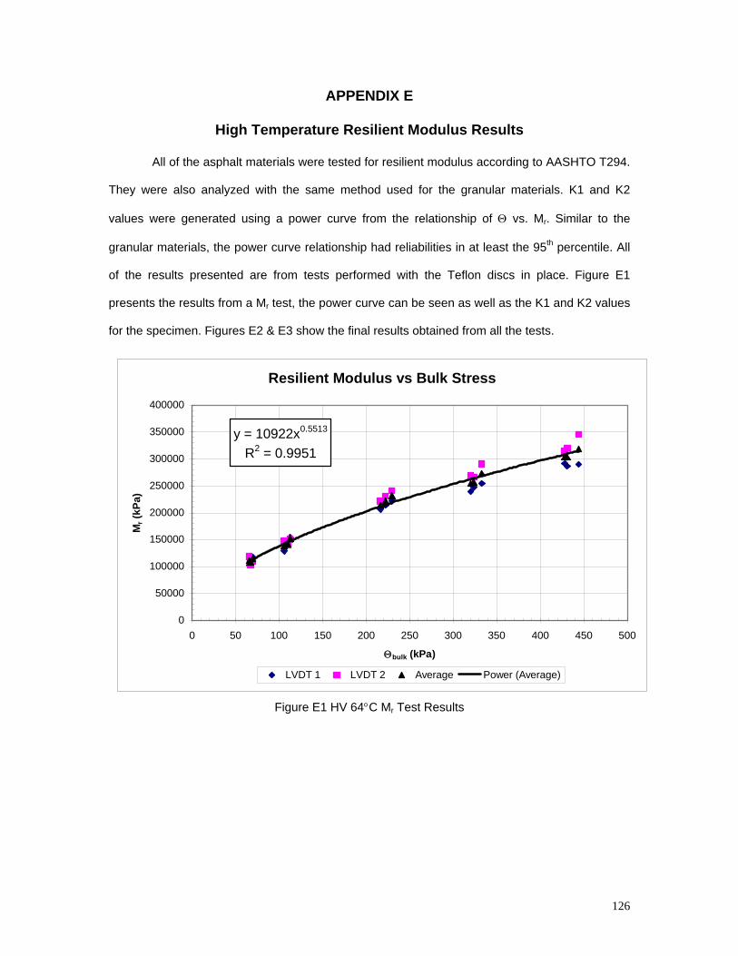
126
APPENDIX E
High Temperature Resilient Modulus Results
All of the asphalt materials were tested for resilient modulus according to AASHTO T294.
They were also analyzed with the same method used for the granular materials. K1 and K2
values were generated using a power curve from the relationship of Θ vs. MBr B. Similar to the
granular materials, the power curve relationship had reliabilities in at least the 95P
thP percentile. All
of the results presented are from tests performed with the Teflon discs in place. Figure E1
presents the results from a MBr B test, the power curve can be seen as well as the K1 and K2 values
for the specimen. Figures E2 & E3 show the final results obtained from all the tests.
Resilient Modulus vs Bulk Stress
y = 10922x0.5513
R2 = 0.9951
0
50000
100000
150000
200000
250000
300000
350000
400000
0 50 100 150 200 250 300 350 400 450 500
Θbulk (kPa)
Mr (
kPa)
LVDT 1 LVDT 2 Average Power (Average)
Figure E1 HV 64°C MBr B Test Results
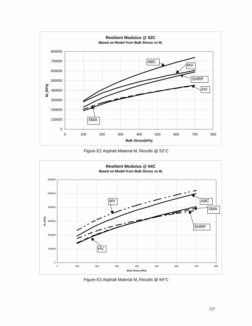
127
Resilient Modulus @ 52CBased on Model from Bulk Stress vs Mr
0
100000
200000
300000
400000
500000
600000
700000
800000
0 100 200 300 400 500 600 700 800
Bulk Stress(kPa)
Mr (
kPa)
SMA
HV
SHRP
ABCMV
Figure E2 Asphalt Material M Br B Results @ 52°C
Resilient Modulus @ 64CBased on Model from Bulk Stress vs Mr
0
100000
200000
300000
400000
500000
600000
0 100 200 300 400 500 600 700 800
Bulk Stress (kPa)
Mr (
kPa)
MV
SMA
HV
SHRP
ABC
Figure E3 Asphalt Material M Br B Results @ 64°C
128
E.1 Material Comparisons
The MBr B data show two trends: the first is that asphalt performs better than granular
materials. The second is that the finer mixes have a higher MBr B. The MV and ABC materials, which
are the finest of all the mixes tested, consistently performed better than the more coarse grained
mixes. The difference over both temperature levels was approximately 20%. The HV mixture and
SMA, which were tested almost identically at both temperatures, were the worst resilient
performers while SHRP fell into the middle. This could suggest that the gradation of the mix
influences the M Br B of an asphalt mixture.
All of the surface materials maintained constant differences between them over the range
of Θ values, except the SHRP mixture. The SHRP mixture at 52°C shows a relatively better
performance at the high Θ values. However, when the same material is tested at 64°C, the
opposite is true ; the performance is relatively poor at high Θ values.
E.2 Temperature Effects
As expected, the temperature caused differences in the M Br B of the materials. The
temperature shift was not always consistent. The HV and SMA showed less of a temperature
dependency than the MV and ABC. The SHRP mixture had the highest temperature shift of all,
especially at high Θ values. This may suggest that materials with a lower M Br B are less
temperature- dependent and vice versa.
Generally, all of the materials show a parallel relation to one another except for SHRP.
The SHRP material also behaves differently at the two temperatures in relation to the other
materials. When tested at 64°C the SHRP, the specimen’s MBr B decreases in relation to the other
tests, but at 52°C the SHRP specimen shows an increasing M Br B.
Finally, in all cases, the M Br B values for the asphalt materials are higher than those of the
recycled granular materials. The factors range from 1.7 at 64°C and 2.2 at 52°C. This trend is not
unusual, nor surprising.
The temperature shifts were used to compare the MBr B results to one another at 20°C and
to current layer coefficient values. Shifting the MBr Bvalues to 20°C allows for the calculation of
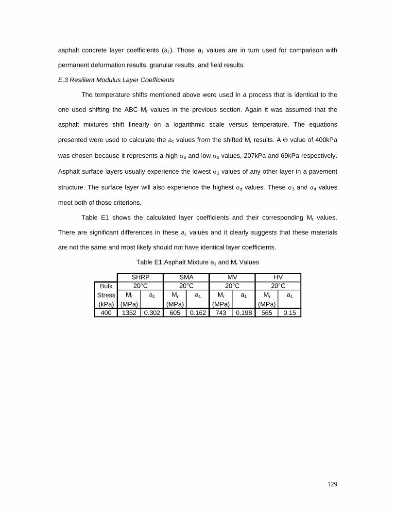
129
asphalt concrete layer coefficients (a B1B). Those a B1B values are in turn used for comparison with
permanent deformation results, granular results, and field results.
E.3 Resilient Modulus Layer Coefficients
The temperature shifts mentioned above were used in a process that is identical to the
one used shifting the ABC MBr B values in the previous section. Again it was assumed that the
asphalt mixtures shift linearly on a logarithmic scale versus temperature. The equations
presented were used to calculate the a B1B values from the shifted MBr B results. A Θ value of 400kPa
was chosen because it represents a high σ BdB and low σ B3B values, 207kPa and 69kPa respectively.
Asphalt surface layers usually experience the lowest σ B3B values of any other layer in a pavement
structure. The surface layer will also experience the highest σ BdB values. These σ B3B and σ BdB values
meet both of those criterions.
Table E1 shows the calculated layer coefficients and their corresponding MBr B values.
There are significant differences in these a B1B values and it clearly suggests that these materials
are not the same and most likely should not have identical layer coefficients.
Table E1 Asphalt Mixture a B1B and M Br B Values
BulkStress Mr a1 Mr a1 Mr a1 Mr a1
(kPa) (MPa) (MPa) (MPa) (MPa)400 1352 0.302 605 0.162 743 0.198 565 0.15
SHRP SMA MV HV20°C 20°C 20°C 20°C
Recommended