Work Incentives and Labor Supply Effects
of the ‘Mini-Jobs Reform’ in Germany
Viktor Steiner *) **) Katharina Wrohlich **)
*) Free University of Berlin **) German Institute for Economic Research (DIW Berlin)
(this version: 23/06/2004)
Abstract: We analyze the work incentives and labor supply effects of the so-called mini-jobs
reform (subsidies of social security contributions to people with low-earnings jobs) introduced
in Germany in April 2003. The analysis is based on a structural labor supply model embedded
in a detailed tax-benefit microsimulation model for which we use the German Socio-
Economic Panel (GSOEP). Our simulation results show that the likely employment effects of
the mini-jobs reform will be small. The small positive participation effect is outweighed by a
negative hours effect among already employed workers. The fiscal effects of the reform are
also likely to be negative. We conclude that the analyzed mini-job reform is not an effective
policy to increase employment of people with low earnings capacity.
JEL classification: J22, H31 Correspondence to: Viktor Steiner DIW Berlin Königin-Luise Strasse 5 D-14195 Berlin, Germany e-mail: [email protected] Acknowledgement: We thank the German Science Foundation (DFG) for financial support under the research programme "Flexibilisierungspotenziale bei heterogenen Arbeitsmärkten" (project STE 681/5-1).

1 Introduction
Recently, wage and earnings subsidies have intensively been discussed in Germany and in a
number of other OECD countries as an instrument of labor market policy (for summaries see,
e.g., Blundell, 2000, Blundell and Hoynes, 2001, Moffitt, 2003). In some European countries
wage subsidies targeted at reducing relatively high social security contributions (SSC) on low
earnings have been introduced to increase employment in low-wage labor markets. There are
basically two arguments for this type of wage subsidies in the economic policy debate: first,
social security contributions on low earnings reduce work incentives of people entitled to
unemployment compensation and means-tested welfare programs, such as social assistance;
second, given limited downward wage flexibility in the low wage sector due to binding
minimum wages, SSC have to be borne at least partially by the employer of low-skilled
workers, thus reducing their employment. Although the structure of the various wage subsidy
schemes already implemented or discussed in various EU countries differ, their main aim is to
increase employment of workers with low earnings potential (OECD, 1999, Steiner, 2003). In
Germany, a SSC subsidy on low earnings has been implemented in 2003 as part of the recent
labor market and social reforms. This SSC subsidy targeted on so-called mini-jobs is part of
the new “welfare-to-work” strategy of the German government (see Steiner and
Jacobebbinghaus, 2003). It is intended to provide positive work incentives for people with
low earnings potential currently living on unemployment benefits or means-tested
unemployment or social assistance.
The effectiveness of wage subsidy schemes in general, and a SSC subsidy in particular,
depends on various economic and institutional factors (see, e.g., Blundell, 2000, Moffitt,
2003). First, the state of the labor market and the degree of wage flexibility will determine to
what extent an increase in the effective supply of labor induced by the SSC subsidy will
actually translate into an employment increase in the low-wage labor market. In the absence
of a substantial number of vacancies for low-wage jobs, employment can only increase if the
wage declines in this sector. Second, although the SSC subsidy will increase work incentives
for currently unemployed people and thus labor force participation, overall labor supply need
not increase, and may even be reduced due to hours adjustment of already employed people.
As the experience with the US Earned Income Tax Credit seems to have shown, this effect is
of special importance for couple households where spouses may adjust their total labor supply
to take advantage of the wage subsidy. In addition to this deadweight loss, there may also be
substantial substitution effects between subsidized and non-subsidized full-time jobs, for
example by splitting up one full-time job into several part-time jobs. Furthermore, given that
1

the wage subsidy is not “self financing” through a net employment increase and thus entails
additional fiscal costs, the financing of these costs by way of increased taxes or SSC may
entail indirect employment losses.
The new mini-jobs law differs in important ways from previous regulations and
proposals for SSC subsidies as a means to increase employment in the low-wage sector in
Germany. The new SSC subsidy is intended to be permanent and not restricted to particular
regions or specific labor market groups, such as the long-term unemployed, the low-skilled or
disabled people. The rather limited knowledge gained from previous evaluation studies on
wage subsidies introduced on a temporary basis or targeted on special groups is, therefore, of
limited use for the evaluation of the new mini-jobs reform. The SSC subsidy also interacts in
a peculiar way with the social welfare system and income taxation. Given the high benefit-
withdrawal rates of means-tested social transfers, the incentive effects of the SSC subsidy
very much depend on pre-reform household income and can only be evaluated on the basis of
a detailed empirical microsimulation analysis.
To analyze the employment and fiscal effects of the mini-jobs reform implemented in
Germany in 2003, we estimate the potential employment effects of this reform on the basis of
a structural labor supply model embedded in a detailed tax-benefit microsimulation model.
The main advantages of this structural microsimulation model are that, first, the incentive
effects of the analyzed mini-jobs reform can be modeled at the individual household level
taking into account the complexities of the German tax-benefit system and, second, effects of
the reform on households’ budget constraints can be separated from preferences for leisure
and income. This also allows us to use our model for the ex-ante simulation of the likely
employment and fiscal effects of the mini-jobs reform under the weak assumption that
household preferences for leisure and income are not affected by the reform.
In the next section, we briefly refer to the on-going German debate on “marginal
employment” (geringfügige Beschäftigung), i.e. “mini-jobs” characterized by a small number
of hours and low earnings previously usually not covered by social security contributions, and
describe the changes introduced by the mini-jobs reform in 2003. In section 3, we present the
empirical methodology to simulate the employment and fiscal effects of this reform, where
the discussion focuses on the econometric specification of our household labor supply model.
Simulation results of the employment and fiscal effects of the recent mini-jobs reform are
contained in section 4. Section 5 summarizes the main results of our study and concludes.
2

2 The German ‘Mini-Jobs Reform’
There has been a prolonged policy debate on the reform of so-called “mini-jobs”
(geringfügige Beschäftigung, or “marginal employment”) in Germany. Before the first reform
in 1999, mini-jobs were exempted from social security contributions (SSC) on the side of the
employee and there was a 20 percent tax on gross wages payable by the employer. Mini-jobs
used to be defined by both an upper earnings threshold (325 € per month) and a maximum of
15 weekly working hours. Before 1999, mini-jobs held as a secondary job by employees were
treated equally with respect to SSC to mini-jobs as the main job. Earnings from several mini-
jobs held by a single person were added-up and the resulting sum was subject to SSC. Since
the 1999 reform the employer had to pay 22 percent SSC (10 percent for public health and 12
percent for public pension insurance). Thus, this reform changed little for the employers of
people working in mini-jobs. On the employee side, the possibility to choose between a 20
percent flat-rate tax on earnings from mini-jobs and taxation according to the income tax code
remained. However, the 1999 reform did not improve financial incentives for workers holding
mini-jobs to expand hours of work and take up regular employment. Since SSC have to be
paid in full above the relatively low SSC threshold and possibly also income taxes, the
marginal tax rate on such jobs is rather high. Even only accounting for SSC contributions,
gross earnings would have to be above 400 € in order to compensate for SSC at the margin.
The political aim of the 1999 reform was to restrict the expansion of mini-jobs which,
according to some estimates (see, e.g., Schupp et al., 1998), had reached between 3 and 5
million cases in the years preceding this reform and to foster employment covered by the
social security system. However, Schwarze und Heineck (2001) conclude on the basis of
their empirical analysis of the 1999 reform that there was no increase in employment covered
by SSC, and that there might have been some substitution between regular employment and
mini-jobs. Furthermore, they find some evidence for employment termination of people
holding mini-jobs before the reform.
In contrast to the 1999 reform, the ’Minijobs-Reform’ of 2003 was intended to boost
employment in the low-wage sector1. The maximum hours restriction was abolished and the
range of exempted earnings was expanded up to 400 €. Furthermore, high marginal tax rates
on incomes above this threshold were decreased. Earnings between 401 and 800 € are now 1 Actually, there shortly existed another legislation between March 2002 and March 2003, called the “Mainzer
Modell”. Under this scheme, which was also meant to subsidize SSC, the subsidy also depended on family status and the number of children. Further, social assistance benefits were not withdrawn at a full rate for people in these jobs. However, in our analysis, we consider the legislation descibed above as the status quo scenario, since the Mainzer Modell was in place only for a short period of time and was initially also intended to be terminated by 2006.
3

subject to a modified SSC scheme. Contributions start at 4 percent and then increase linearly
up to the normal rate of 21 percent at the end of the bracket. Above 800 €, SSC are due on the
whole amount of gross earnings. Table 1 summarizes the changes in employees’ SSC due to
the 2003 reform.
Table 1: Changes in employee’s SSC due to the Minijobs-Reform 2003 Before April 2003 After the Reform
Exemption of income tax and social security contributions up to…
325 Euro 400 Euro
Full social security contributions set in at… 326 Euro
801 Euro
subsidies to SSC for earningsbetween 401 and 800 Euro
Income tax sets in at …
326 Euro 401 Euro
Maximum hours restriction
15 hours per week none
Employers have to pay SSC of 25 percent of the employee’s wage for earnings up to
400 €2. Between 401 and 800 €, employers pay the normal rate of 21 percent. Employees are
covered by health insurance, however, they do not aquire further social security entitlements.
Employees can choose to individually add up the SSC to the normal rate in order to be
entitled to benefits of the old age insurance. Earnings up to 400 € are taxed by a flat rate of 2
percent.
Net monthly incomes before and after the reform are shown in Figure 1 for two
household types. In case of the single household, it is assumed that the employee has no other
income. This figure shows, that the drop in the pre-reform curve is moved to the right and
flattened after the reform. However, for a married couple, where the primary earner is
assumed to have a gross monthly income of 3,000 €, there is still a considerable decline in net
household income at a secondary income above 400 €. This remaining drop in the budget line
of a married couple is due to the fact that after 400 €, also income from the secondary earner
is fully subject to income tax under the joint taxation with income splitting (see Steiner and
Wrohlich, 2004). At this point, the marginal tax rate is very high, the exact rate depending on
the primary earner’s income.
2 For people employed by private households, social security contributions are even more subsidized. In case
the employer is a private person, he only has to pay social security contributions of 12 percent (instead of 25 percent) of the employee’s wage.
4
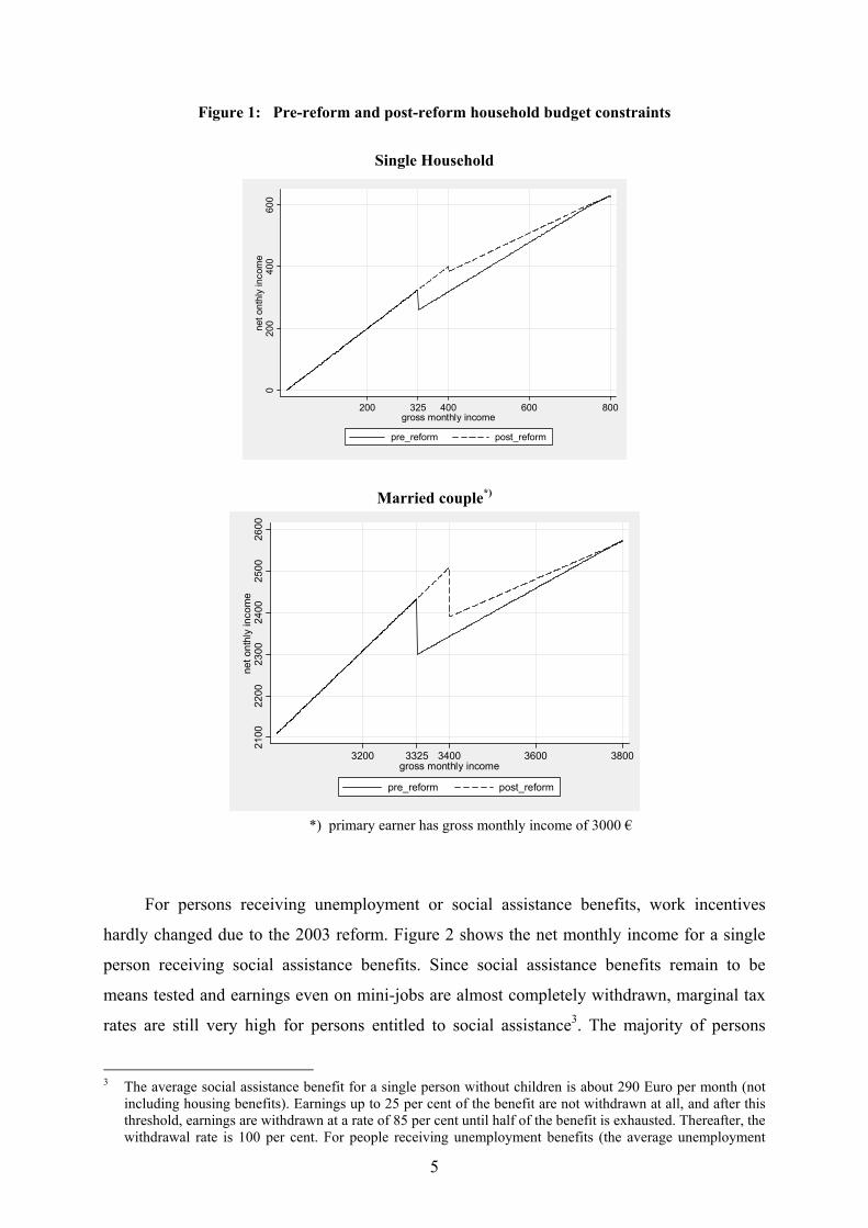
Figure 1: Pre-reform and post-reform household budget constraints
Single Household
020
040
060
0ne
t ont
hly
inco
me
200 325 400 600 800gross monthly income
pre_reform post_reform
Married couple*)
2100
2200
2300
2400
2500
2600
net o
nthl
y in
com
e
3200 3325 3400 3600 3800gross monthly income
pre_reform post_reform
*) primary earner has gross monthly income of 3000 €
For persons receiving unemployment or social assistance benefits, work incentives
hardly changed due to the 2003 reform. Figure 2 shows the net monthly income for a single
person receiving social assistance benefits. Since social assistance benefits remain to be
means tested and earnings even on mini-jobs are almost completely withdrawn, marginal tax
rates are still very high for persons entitled to social assistance3. The majority of persons
3 The average social assistance benefit for a single person without children is about 290 Euro per month (not
including housing benefits). Earnings up to 25 per cent of the benefit are not withdrawn at all, and after this threshold, earnings are withdrawn at a rate of 85 per cent until half of the benefit is exhausted. Thereafter, the withdrawal rate is 100 per cent. For people receiving unemployment benefits (the average unemployment
5
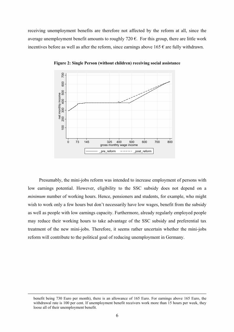
receiving unemployment benefits are therefore not affected by the reform at all, since the
average unemployment benefit amounts to roughly 720 €. For this group, there are little work
incentives before as well as after the reform, since earnings above 165 € are fully withdrawn.
Figure 2: Single Person (without children) receiving social assistance
100
200
300
400
500
600
700
net m
onth
ly in
com
e
0 73 145 325 400 500 600 700 800gross monthly wage income
_pre_reform _post_reform
Presumably, the mini-jobs reform was intended to increase employment of persons with
low earnings potential. However, eligibility to the SSC subsidy does not depend on a
minimum number of working hours. Hence, pensioners and students, for example, who might
wish to work only a few hours but don’t necessarily have low wages, benefit from the subsidy
as well as people with low earnings capacity. Furthermore, already regularly employed people
may reduce their working hours to take advantage of the SSC subsidy and preferential tax
treatment of the new mini-jobs. Therefore, it seems rather uncertain whether the mini-jobs
reform will contribute to the political goal of reducing unemployment in Germany.
benefit being 730 Euro per month), there is an allowance of 165 Euro. For earnings above 165 Euro, the withdrawal rate is 100 per cent. If unemployment benefit receivers work more than 15 hours per week, they loose all of their unemployment benefit.
6

3 Simulation Methodology
In this section, we describe our methodology to simulate the employment and fiscal effects of
the mini-jobs reform outlined in the previous section. Since this reform is intended to improve
incentives to take up jobs at low earnings and thus increase effective labor supply, the natural
starting point for the ex-ante evaluation of this reform is the supply side. Of course, given an
estimate of the potential labor supply effects of the reform, the corresponding employment
effects will depend on the way labor demand and wages adjust in the respective labor
markets. We will return to this issue below when discussing our simulation results.
In order to estimate the labor supply effects of the mini-jobs reform, we extend previous
work (Steiner 2000, Steiner and Wrohlich 2004) and integrate a household labor supply
model with a detailed tax-benefit microsimulation model. The budget constraints of
households are extremely complicated due to the complexities of the German tax and transfer
system, especially the joint income taxation of spouses and the means tested social assistance
scheme. Therefore, a detailed specification of the household’s budget constraint seems crucial
when analyzing the incentive effects of the social security contributions subsidies.
3.1 Econometric Specification
We model the labor supply decision of individuals in the household context according to the
household utility model (see van Soest 1995). This model is based on the assumption that
both spouses jointly maximize a utility function in the arguments leisure of both spouses and
net household income.4 Hours of work are assumed to be a categorical rather than a metric
variable. This form of modeling takes into account the fact that hours of work are heavily
concentrated at particular hours. The most important reason for this kind of modeling,
however, is that the specification of a relatively small number of hours categories leads to a
substantial reduction in computational burden, as the budget set of a household has to be
computed for several selected points only. Therefore, this simplification is in fact a
prerequisite for an adequate specification of the budget constraints given the complexitites of
the German tax-benefit system.
Following van Soest (1995), we specify a household utility function depending on the
leisure time of the household members and net household income. We assume that the
household’s utility index for a particular hours category k can be modelled by the following
translog function: 4 It is assumed that the labor supply decisions of the household head and spouse can be separated from the
labor supply decision of all other household members. The labor supply decision of single persons can be seen as a special case of the couple’s labor supply decision.
7

(1) kkkkkk xAxxxU εβ ++= '')(
where x = (y, lm, lf)’. The components of x are the natural logs of net household income (y),
leisure of the husband (lm) and leisure of the wife (lf). These components enter the utility
function in linear, quadratic and cross terms. The matrix A, with elements αij, i,j = (1,2,3),
contains the coefficient of the quadratic and the cross terms, the vector βj, j = (1,2,3), the
coefficients of the linear terms. εk is a stochastic error term accounting for unobserved factors
that affect household utility, its distribution is specified below.
The utility index should be concave in household income and, for given household
income, be increasing in both spouses’ leisure time (provided working hours were initially
positive). Moreover, the first derivative of the utility index with respect to leisure time should,
ceteris paribus, be positive for both spouses, provided leisure is a normal good, while the
second derivative should be negative. In the HU model, the cross-substitution effect between
the two spouses’ leisure time is theoretically ambiguous. That is,
(2)
?;)(?;)(;0)(;0)(
;0)(;0)(
;0)(;0)(
2
2
2
2
2
2
=∂∂⋅∂
=∂∂⋅∂
<∂
⋅∂<
∂⋅∂
>∂
⋅∂>
⋅
<∂
⋅∂>
∂⋅∂
fmmfmf
mf
llU
llU
lU
lU
lU
lU
yU
yU
∂∂
These theoretical implications can be tested by calculating respective derivatives of the utility
index for each household evaluated at the parameter estimates from the econometric model
described below. The sign of the cross effects depend on whether the two spouses’ leisure
times are substitutes or complements and can only be determined empirically.
Given the assumption of joint maximization of household utility, the household will
choose hours category k if, in probability terms, the associated utility index, Uk, exceeds the
utility index in any other possible alternative l, i.e.:
(3) ( ) ( )[ ]kllllkkklk xAxxxAxxPUUP εεββ −>+−+=> '''')( .
8

Assuming that εk is distributed identically across all hours categories according to an extreme-
value distribution5, the difference of the utility index between any two hours categories
follows a logistic distribution. Under this distributional assumption the probability of
choosing alternative k relative to alternative l can be described by a Conditional Logit Model
as introduced by McFadden (1973):
(4) ,,)''exp(
)''exp()( kl
xAxxxAxx
UUP
mmmm
kkklk ≠∀
++
=>∑ β
β
where the summation sign is defined over all possible alternatives, i.e. hours categories. We
control for observed heterogeneity by accounting for household characteristics such as age
and health status of both spouses, number and age of children in the household, regional and
nationality variables. Because variables with no variation across alternatives drop out of the
estimation in the conditional logit model, the household-specific variables are interacted with
household income and leisure times which vary across hours categories.
3.2 Data
Estimation of our labor supply model outlined in the previous section is based on data from
the most recent wave (the year 2002) of the German Socio-Economic Panel (GSOEP)6. The
GSOEP is a representative sample of private households living in Germany with detailed
information on household incomes, hours worked and household structure. This information
is required for both, the estimation of the labor supply model and the calculation of
hypothetical levels of net household incomes at the different hours categories before and after
the reform. Since we want to analyze the labor supply responses reaction to the reform for the
“main” labor force, we restrict our sample to household members between 20 and 65 years
who are not pensioners and not in any sort of schooling, training or university any more. Also
self-employed people and civil servants are excluded, since these groups might differ in their
labor supply behaviour. Descriptive statistics on some key variables are given in the appendix.
5 The assumption that the error terms following an extreme value distribution is rather restrictive and results in
the property of the independence of irrelevant alternatives. Random coefficient models, as opposed to the conditional logit model we use here, allow for unobserved heterogeneity and therefore circumvent this ’IIA-assumption’. However, Haan (2003), who estimated several labor supply models with the same data set we do, showed that the results (in terms of wage elasticities) from a random coefficient model did not differ significantly from the results obtained from a conditional logit model.
6 Although we use data from the year 2002, simulations are undertaken for the year 2001. The reason is, that most income variables we use are retrospective calendar data from the GSOEP referring to the year 2001.
9

We run separate estimations for couple households, single men and single women. For
technical reasons, we further divide couple households in three groups, those where both
spouses are assumed to be flexible regarding their labor supply behavior (i.e. both spouses are
neither pensioners, nor students, nor in maternity leave, nor civil servants or self-employed),
those where only the husband is assumed to be flexible and those where only the wife is
assumed to be flexible. This is an extension of our previous work, where we included only
couple households with two flexible spouses in our sample. By including these types of
households in our analysis, we are able to provide a more accurate picture of the quantitative
size of the labor market effects of the reform under consideration.
Hours Categories
In the GSOEP, information on the number of weekly hours actually worked (thus including
overtime) in the month before the interview is given. The definition of the hours categories is
motivated by both, economic considerations and the actual distribution of hours in the sample.
Although a relatively fine aggregation of hours into categories seems desirable in order to
realistically approximate the household’s budget constraint, the actual distribution of hours in
the sample severely restricts the number of possible categories. In particular, men in our
restricted sample typically do not work part-time and their actual working hours are heavily
concentrated between 35 and 40 hours per week. For women, we extend the hours categories
set that we used in previous applications in order to capture the possible effects of the mini-
jobs reform7. Table 2 shows the distribution of couple and single households across hours
categories.
Because of the small number of men in part-time employment in our sample, only three
categories could be specified for them, namely non-employment (unemployment and non-
participation in the labor force), 1-40 hours and more than 40 hours (overtime)8. For women
we specify six hours categories: non-employment, three part-time categories, full time and
overtime.
The specification of the econometric model is based on the assumption that each
household compares the expected utility obtained from net income and the two spouses’ (or,
7 A comparison of several estimations with different numbers of hours categories showed, that the results of
the labor supply estimation in terms of wage elasticities are not very sensitive to the number of hours categories. The labor supply effects of the reform considered in this paper, however, differ significantly according to the number of hours categories, since a household’s budget constraint at different hours of part-time work changes considerably due to the reform.
8 It should be noted that without modelling a part-time category for men, the effects of the mini-jobs reform for this group are necessarily small, as only for men with a very low hourly wage rate the net household income in the full-time category changes due to the reform.
10

in the case of singles, the person’s) leisure associated with the choice of a particular hours
category. Here, it is assumed that this comparison is based on the average number of hours
worked in a particular hours category, where leisure is calculated by subtracting the working
hours from an assumed total time of 80 hours per week.
Table 2: Distribution of households among hours categories Couples, both spouses flexible hours Men
Weekly Hours* 0 1-40 (37) > 40 (48) Sum 0 200 (5.7)** 526 (14.9) 409 (11.6) 1135 (32.2) 1-12 (8.5) 211 (6.0) 131 (3.7) 13-20 (18) 239 (6.8) 159 (4.5) 21-34 (27)
88 (2.5) 294 (8.3) 206 (5.8)
1328 (37.6)
35-40 (38.5) 490 (13.9) 250 (7.1) >40 (45)
108 (3.1) 101 (2.9) 125 (3.5)
1074 (30.5)
Wom
en
Total 396 (11.3) 1861 (52.8) 1280 (36.2) 3537 * Average of weekly working hours in parentheses ** Relative share in parentheses Couples, only one spouse flexible hours
Men Women Weekly Hours of Man (Woman not flexible)
Weekly Hours of Woman (Man not flexible)
0 70 (11.24) 0 483 (37.68) 1-12 (8.5) 80 (6.24) 13-20 (18) 211 (16.46) 21-34 (27) 140 (10.92) 1-40 (36.5) 284 (45.59)
35-40 (38.5) 293 (22.85) > 40 (47) 269 (43.18) >40 (47) 75 (5.85) Total 623 Total 1282
Singles
Men Women Weekly Hours Weekly Hours 0 133 (17.7) 0 301 (28.5)
1-12 (7.5) 44 (4.2) 13-20 (18) 61 (5.8) 21-34 (28) 133 (12.6) 1-40 (37) 399 (53.0)
35-40 (38.5) 386 (36.6) > 40 (48) 221 (29.4) >40 (46) 130 (12.3) Total 753 Sum 1055
Source: GSOEP, wave 2002 Net Household Income
Net household income for all hours categories and for the policy regime before and after the
reform are calculated by applying a detailed tax-benefit simulation model wich includes the
main features of the German tax and transfer system. The calculation of taxable income is
11

based on information on earnings from dependent employment, income from capital, property
rents and other income. For most households, earnings from dependent employment is the
most important source of income. These earnings are calculated by multiplying gross hourly
wages by the respective working hours in each hours category. For non-working individuals,
wages are estimated by applying a two-stage estimation with a Heckman (1979) sample
selection correction9. Estimation results for the wage equations are available from the authors
upon request.
Gross household income is calculated by adding all income components of all
household members (weekly working hours are only varied by category for the head of the
household and the spouse). Taxable income is calculated by deducting certain expenses from
gross household income. The income tax is computed by applying the income tax formula to
taxable income of each person in the household or of the spouses’ joint income, depending on
marital status. Then, the income tax and employee’s social security contribution rates are
deducted from gross income, and social transfers are added to get net thousehold income.
Social transfers include child benefits / allowances, child-rearing benefits, education benefits
for students (BAfoeG), unemployment compensation, housing benefits and social assistance.
From this simulated net household income, we further deduct costs of child care. Based
on information about child care expenditures in the GSOEP, we estimate hourly child care
costs for households with preschool children and deduct these costs according to the mother’s
working hours. For details on the child care costs estimation see Wrohlich (2004)10.
Other Variables Describing Household Preferences
Household preferences for leisure and income may differ by some observable household
characteristics such as region (east or west Germany), nationality, age and disability status of
household members as well as the number of children. We control for these variables by
including interaction terms of these variables with the leisure terms in the conditional logit
model. Thus, we allow the effect of any of these variables on household utility to vary across
hours categories.
9 In order to increase the variance of predicted wages to make it comparable to that of observed wages, we
adjust the predicted wages by adding the normalized error term distribution of the regression of the observed wages.
10 The results of the estimation are available from the authors upon request.
12

4 Simulation Results
The following presentation of our simulation results proceeds in three steps. In the next
section we describe the effects of the mini-jobs reform on net household income without
account for behavioral effects. In section 4.2 we present and discuss the simulated labor
supply effects of the reform, and in section 4.3 we report on its expected fiscal effects.
4.1 Changes in Net Household Income
The mini-jobs reform changes net household income for households where one person has
income from dependent employment between 325 and 800 € per month. Most people earn
income in this range when working part time, although there are some persons with very low
wages who do not earn more than 800 € even if they work full time. Since we also take into
account income from other household members (adult children etc.) when calculating certain
household benefits, net household income might also change due to changes in the income of
other family members11. These income changes, however, are rather small and are the same
for all hours categories, since we do not vary the hours of household members other than the
head of the household and the spouse.
The changes in net household income due to the mini-jobs reform are presented in Table
3. As expected, average net household income does not change in categories with high
working hours. In couple households as well as for single women, income changes in two
part-time categories only. As we do not model part-time categories for single men, there is –
by definition, effectively – no income change for this group. In Table 4, we present the
income changes for those groups who are affected by the reform (all households in which the
woman is working part time) in more detail.
These average income changes listed by hours categories, however, do not show one
important result of the mini-jobs reform: For seven percent of all couple households (three
percent of all households of single women), net household income actually declines when the
woman switches from 8.5 to 18 hours. The loss in net household income in these cases is
between 30 and 50 € per month.
11 Income of other household members, such as adult children, does not directly enter the utility function of the
household in our model. However, as certain household benefits, e.g. social assistance and housing benefits, depend on the income of all household members, these transfers might be reduced for certain households as a result of the reform.
13

Table 3: Income changes by hours category (in € per month) Couples with two flexible spouses Couples, only woman flexible Single Women
Working Hours Average Income Change
Working Hours of Woman
Average Income Change** Working Hours Average Income
Change 0/0, 0/37, 0/48* 0 0 1 0 0
8.5/37, 8.5/48 50 8.5 38 7.5 16
18/37, 18/48 8 18 11 18 6
27/37, 27/48 0 27 5 28 0
38.5/37, 38.5/48 0 38.5 3 38.5 0
45/37, 45/48 0 47 2 46 0
19/0 6
40/0 0 *First number refers to hours of the wife, second number to average hours of the husband. ** These households face income changes also in categories with zero or high working hours of the woman since the
husband, whose hours are fixed, might have an income between 325 and 800 Euro.
Source: GSOEP, wave 2002, simulation results. Table 4: Income changes for selected groups (in € per month)
Couples with two flexible spouses
Couples, only woman flexible Single Women
Income Change at Working Hours 8.5/37* and 8.5/49*
Income Change at Woman’s Working Hours 8.5
Actual Income Change at Working Hours 8.5
Minimum -12** -3** -39** 1st Quartile 0 0 0 Median 1 21 0 3rd Quartile 57 41 11 Maximum 260 231 150
Income Change at Working Hours 18/37* and 18/49*
Income Change at Woman’s Working Hours 18
Income Change at Working Hours 18
Minimum -18** -7** -3** 1st Quartile 0 0 0 Median 0 0 0 3rd Quartile 0 11 4 Maximum 179 255 56 *First number refers to hours of the wife, second number to average hours of the husband. ** Negative income changes may occur due to withdrawal of other transfers such as housing benefits or social assistance.
Source: GSOEP, wave 2002, simulation results.
14

4.2 Labor Supply Effects
Since the net household income in part-time categories rises, also the probability that the
utility index in these categories exceeds the utility index in hours categories where the woman
is not working, rises. Therefore we expect a positive change in the participation rate of
women. However, as part-time categories also become more attractive relative to full-time
categories, we also expect some women to switch from working full time to part time. The
conditional hours effect of those who are already working is therefore expected to be
negative. The sign of the total hours effect depends on which of the two opposing effects is
dominating.
We present the labor supply effects in Table 5. As expected, there is an increase in the
participation rate. The highest increase in the participation rate occurs for women in couple
households – their participation rate rises by 0.3 percentage points. For married men and
single women, the rise is even smaller. Those people, who were already employed before the
reform, reduce their working hours. The conditional hours effect is significant only for
women: they reduce their working hours by 0.7 percent. The effect on total hours (the hours
effect of those already working plus the hours effect of those starting to work after the reform)
is also negative for women in couple households. This implies that the total hours reduction
by the women already working dominates the participation effect in terms of hours of the
women who start to work after the reform. For single women, however, the total hours effect
is positive.
Applying the GSOEP weighting factors that come along with each observation (on the
household and on the individual level), allows to calculate aggregate numbers of the labor
supply effects. In Table 6, we show the total number of persons who start to work after the
reform, the hours effect due to additional participation, the hours effect of those already
working before the reform and the total hours effect. Total participation rises by about 53,000
persons (about 36,000 full-time equivalents). The total hours effect, however, is negative,
since those people who are already working, reduce their hours (this negative conditional
hours effect is as large as 37,500 full-time equivalents).
It seems save to assume that the small estimated number of about 50,000 additional
people who are induced by the mini-jobs reform to take up work will get employed, given the
relatively large number of job vacancies even in times of weak aggregate demand and the
estimated reduction in the supply of total working hours. Hence, we will assume that labor
demand adjusts flexibly to small changes in labor supply and equate the labor force
participation effect to the employment effect.
15

Table 5: Labor supply effects of the mini-jobs reform
Couples, Both Spouses Flexible
Couples, only one spouse flexible
Singles
Women Men Women Men Women Men
Change in the participation rate (in percentage points)
All couples/All singles 0.32 (0.24 – 0.38)*
0.07 (0.06 – 0.09)
0.23 (0.16 – 0.31)
0.08 (0.04 – 0.14)
0.05 (0.02 – 0.07) 0.00
West Germany 0.38 (0.32 – 0,46)
0.08 (0.07 – 0.10)
0.25 (0.17 – 0.33)
0.07 (0.04 – 0.12)
0.05 (0.02 – 0.09) 0.00
East Germany 0.11 (0.06 – 0.15)
0.06 (0.04 – 0.08)
0.16 (0.10 – 0.23)
0.13 (0.01 – 0.29)
0.05 (0.02 – 0.07) 0.00
Conditional hours effect (in percent)
All couples/All singles -0.74 (-0.86 – -0.54)
0.01 (0.005 – 0.01)
-0.41 (-0.54 – -0.28)
0.13 (0.06 – 0.22)
-0.16 (-0.23 – -0.09) 0.00
West Germany -0.87 (-1.03 – -0.61)
0.01 (0.006 – 0.01)
-0.44 (-0.55 – -0.30)
0.10 (0.05 – 0.18)
-0.17 (-0.24 – -0.09) 0.00
East Germany -0.30 (-0.40 – -0.18)
0.00 (0.001 – 0.01)
-0.27 (-0.39 – -0.18)
0.21 (0.00 – 0.43)
-0.14 (-0.27 – -0.07) 0.00
Change in total hours worked (in percent)
All couples/All singles -0.09 (-0.14 – -0.01)
0.11 (0.08 – 0.13)
0.10 (0.08 – 0.12)
0.01 (0.00 – 0.01)
0.09 (0.03 – 0.16) 0.00
West Germany -0.08 (-0.13 – 0.01)
0.11 (0.09 – 0.14)
0.11 (0.08 – 0.12)
0.00 (0.00 – 0.01)
0.11 (0.05 – 0.19) 0.00
East Germany -0.12 (-0.18 – -0.07)
0.09 (0.06 – 0.13)
0.01 (-0.11 – 0.08)
0.01 (0.00 – 0.02)
0.01 (-0.09 – 0.11) 0.00
* Numbers in parentheses refer to 95-percent bias-corrected bootstrap confidence intervals (100 repetitions).
Source: GSOEP, wave 2002, simulation results. Table 6: Labor supply effects: aggregate numbers (in thousands)
Number of Persons
additionally participating
after the reform
Total hours effect (per week)
Hours effect due to additional participation
(per week)
Conditional hours effect
(per week)
Women 42* (31 – 52)**
-409 (-829 - 11)
957 (727 – 1,187)
-1,367 (-1,719 – -1,014)
Couples Men 9
(7 – 12) 412
(305 – 520) 381
(289 – 474) 31
(13 – 49) Women 2
(1– 4) -82
(-125 – -40) 58
(30 – 87) -140
(-253 – -94) Singles Men 0 0 0 0
Total 53 (40 – 67)
-79 (-127 – -32)
1,396 (1,044– 1,747)
-1,476 (-1,970 – -930)
* Rounded to the nearest thousand. ** Numbers in parentheses refer to 95-percent bias-corrected bootstrap confidence intervals (100 repetitions). The confidence intervals of the sums were computed by calculating a weighted average of the percentage deviation of the bounds of the confidence intervals from the mean. Source: GSOEP, wave 2002, simulation results.
16

However, several limitations of our analysis should be noted at this point: As already
mentioned, we focus only on the group we define as the “main” labor force and therefore
cannot quantify the effects the reform has on the behavior of students or pensioners. Further,
due to reasons of simplification, we only model the labor supply effects of heads of
households and their spouses. Behavioral changes of other household members are not
analyzed. Last but not least, we do not model the possibility of employed individuals to take
up a mini-job in addition to other employment. In our model, when individuals switch to a
higher hours category, their income from dependent employment is increased and income tax
and social security contributions are calculated on the basis of the higher income. Therefore,
we probably underestimate the total hours effect, since under the new legislation, taking on a
secondary job becomes more attractive as there are several advantages in terms of income tax
when the secondary job is defined as mini-job.
It has been argued that one of the aims of the “Minijobs-Reform” was the reduction of
employment in the shadow economy. Combating illicit work is also a popular argument for
subsidizing employers’ SSC on jobs in private households. However, as we have argued in
section 2, as far as the labor supply side is concerned, the incentives to transform illicit work
into legal contracts were not changed significantly. Therefore we doubt that the reform will
have a large effect also in this respect.
4.3 Fiscal Effects
Given the effect on aggregate labor supply is negative, there might be substantial fiscal costs
of the reform which have to be financed by increasing taxes or SSC, or both. This might lead
to further reduction in the aggregate supply of labor. Even if the estimated total hours effect
of the reform is rather small, income tax receipts and social security contributions will decline
as a result of the reduction in working hours of the people already working before the reform.
These losses will not be compensated completely by taxes and social contributions paid by
people induced by the reform to take up a mini-job. These individuals will choose hours that
are in the range of the mini-jobs, therefore paying no or very low social security contributions
(at least on the employee’s side).
Table 7 shows the aggregate effects on income tax and social security contributions.
The aggregate amount of income tax decreases by 0.25 billion € per year. It should be noted,
however, that in some cases earnings of mini-jobs are taxed by a two percent flat rate, which
we did not consider in our simulations. The decrease in the amount of income tax is therefore
overestimated. Employees’ social security contributions decrease by 0.81 billion € per year.
17

We do not calculate employer’s social security contributions, but one should keep in mind
that they will not decrease by the same amount, since employers pay contributions of 25
percent of the earnings of people holding a mini-job.
Table 7: Aggregate fiscal effects (in millions of € per year) Changes in Income Tax
Effect without
behavioral change Effect due to
behavioral changeTotal effect Number of
households (in millions)
Couples -244 (-412 – -76)
-105 (-170 – -40)
-351 (-575 – -127) 15.1
Single men 0 0 0 3.7
Single women -5 (-10 – -1)
-14 (-21 – -6)
-19 (-28 – -10) 4.8
Totals -249 (-398 – -100)
-119 (-180 – -58)
-370 (-554 – -186) 23.6
Changes in Social Security Contributions (Employee’s Contributions Only)
Effect without behavioral change
Effect due to behavioral change Total effect Number of persons
(in millions) Couples: Men -2
(-7 – 3) +53
(24 – 82) +52
(23 – 81) 15.3
Couples: Women -633 (-771 – -495)
-104 (-160 – -48)
-738 (-907 – -569) 15.7
Single men 0 0 0 3.7
Single women -109 (-135 – -83)
-16 (-24 – -8)
-125 (-156 – -94) 5.2
Totals -744 (-1,494 – 6)
-67 (-99 – -35)
-811 (-1,062 – -560) 39.9
* Numbers in parentheses refer to 95-percent bias-corrected bootstrap confidence intervals (100 repetitions). The confidence intervals of the sums were computed by calculating a weighted average of the percentage deviations.
Source: GSOEP, wave 2002, simulation results.
As mentioned above, many students and pensioners might find it attractive to take up a mini-
job, and some employed persons might take up a mini-job as secondary employment.
Therefore, the losses in the social security contributions will be lower in the aggregate.
However, for the group of people defined in this study, the effects of the mini-jobs reform in
terms of income tax and social security contributions are negative although we find a positive
effect on the participation rate.
18

To assess the overall fiscal balance, also unemployment and social assistance benefits of
people taking up a mini-job have to be taken into account. The maximum monthly net income
that can be achieved with a mini-job is 650 €. This is about the social assistance benefit for a
single person (including housing and other in-kind benefits) and below the average of
unemployment benefits. Thus, it is not likely that persons who are eligible for these benefits
will take up a mini-job. Therefore it seems save to argue that the potential savings due to
lower social assistance or unemployment benefits claims will be small, if they exist at all.
5 Summary and Conclusion
We have analyzed the employment and fiscal effects of the so-called mini-jobs reform
introduced in Germany in April 2003. This reform is intended to improve work incentives for
people with low earnings capacity by subsidizing social security contributions on mini-jobs. It
is considered an important component of the German government’s new “welfare-to-work”
strategy. Our ex-ante evaluation of this reform is based on a structural labor supply model
embedded in a detailed tax-benefit microsimulation model. The main advantages of this
structural microsimulation model are that, first, the incentive effects of the analyzed mini-jobs
reform can be modeled at the individual household level taking into account the complexities
of the German tax-benefit system and, second, effects of the reform on households’ budget
constraints can be separated from preferences for leisure and income. This also allows us to
use our model for the ex-ante simulation of the likely employment and fiscal effects of the
mini-jobs reform under the weak assumption that household preferences for leisure and
income are not affected by the reform.
Our simulation results show that the likely employment effects of the mini-jobs reform
will be small. We estimate that total labor force participation will increase by 50,000 persons,
or about 36,000 full time equivalents, which would also be the maximum employment effect
of the reform. This small positive participation effect is outweighed by a negative hours effect
among already employed workers. In terms of full-time equivalents, this negative conditional
hours effect outweighs the positive participation effect. Hence, the net employment effect of
the mini-job reform is slightly negative. This also implies a negative net fiscal effect of the
reform. The aggregate reduction of income tax receipts and employees social security
contributions amounts to about 1 billion € per year. The overall fiscal effect will be somewhat
reduced by additional taxes and social security contributions paid by employers on mini-jobs,
but it seems unlikely that this will compensate fully for the former effect.
19

We therefore conclude that the employment and fiscal effects of the mini-jobs reform
are unlikely to be positive, at least for the population we have defined as the “main” labor
force. Since this definition excludes students and pensioners, for whom the mini-jobs reform
improves incentives to work a few hours, we probably underestimate the labor force
participation and total hours effects. However, from a labor market perspective a mini-jobs
reform which reduces total employment of the “main” labor force and increases employment
of pensioners and students can hardly be considered a success.
20

References
BLUNDELL, R. (2000): Work Incentives and ‘In-Work’ Benefit Reforms: A Review, Oxford Review of Economic Policy, 18, 27 – 44.
BLUNDELL, R., H. HOYNES (2001): “Has ‘In-Work’ Benefit Reform Helped the Labor Market?”, NBER Working Paper 8546, Cambridge, Mass.
HAAN, P. (2003): "Discrete Choice Labor Supply: Conditional Logit Vs. Random Coefficient Models," DIW Discussion Paper 394, Berlin.
MCFADDEN, D. (1973): "Conditional Logit Analysis of Qualitative Choice Behavior," in Frontiers in Econometrics, ed. by P. Zarembka: Academic Press.
MOFFITT, R. (2003): Welfare Programs and Labor Supply, NBER Working Paper 9168, Cambridge, Mass.
OECD (1999), Implementing the OECD Jobs Strategy – Assessing Performance and Policy, Paris.
SCHUPP J., J. SCHWARZE and G. WAGNER (1998): „Methodische Probleme und neue empirische Ergebnisse für die Messung der geringfügigen Beschäftigung“, in: J. Schupp et al. (eds.), Arbeitsmarktstatistik zwischen Fiktion und Realität, Berlin.
SCHWARZE J. and G. HEINECK (2001): „Auswirkungen der Einführung der Sozialversicherungspflicht für geringfügig Beschäftigte – Eine Evaluation des „630-DM-Jobs“-Reformgesetzes“, DIW Diskussionspapier 257, Berlin.
STEINER, V. (2000): "Können durch einkommensbezogene Transfers an Arbeitnehmer die Arbeitsanreize gestärkt werden? Eine ökonometrische Analyse für Deutschland," Mitteilungen aus der Arbeitsmarkt- und Berufsforschung, 33, 385-395.
STEINER, V. (2003): "Beschäftigungseffekte einer Subventionierung der Sozialbeiträge von Geringverdienern," in Wechselwirkungen zwischen sozialer Sicherung und Arbeitsmarkt, ed. by W. Schmähl. Berlin: Duncker & Humblot, 11-44.
STEINER, V. and P. JACOBEBBINGHAUS (2003): "Reforming Social Welfare as We Know It? A Microsimulation Study for Germany“, Mimeo, Berlin, www.fu-berlin.de/wifo/social_reform.pdf.
STEINER, V. and K. WROHLICH (2004): "Household Taxation, Income Splitting and Labor Supply Incentives. A Microsimulation Study for Germany," DIW Discussion Paper 421, Berlin.
VAN SOEST, A. (1995): "Structural Models of Family Labor Supply: A Discrete Choice Approach," Journal of Human Resources, 30, 63-88.
WROHLICH, K. (2004): "Child Care Costs and Mother’s Labor Supply: An Empirical Analysis for Germany," DIW Discussion Paper 412, Berlin.
21

Appendix Table A1: Sample size by group
Group Sample Size Couples with two flexible spouses 3,537 Mixed couples: woman flexible 1,518 Mixed couples: man flexible 631 Single women 1,055 Single men 753 Total 7,494
Table A2: Average simulated net household income by hours category (in € per month)
Couples with two flexible spouses
Couples, only woman flexible Couples, only man flexible
Hours Category
Average Household
Income
Hours Category
Average Household
Income
Hours Category
Average Household
Income 0/0* 1320 0** 2679 0*** 1573 19/0 1684 8.5 4094 36.5 3169 40/0 2011 18 3478 47 4325 0/37 2492 27 4077
8.5/37 2705 38.5 3930 18/37 3035 47 4097 27/37 3082
38.5/37 3205 45/37 3465 Single Women Single Men 0/48 3473 0 921 0 638
8.5/48 3863 7.5 1171 37 1692 18/48 4016 18 1326 48 2218 27/48 3904 28 1460
38.5/48 3839 35.8 1640 45/48 4466 46 1886
* First number refers to hours of the woman, second number to average hours of the men. ** Number refers to working hours of the woman. *** Number refers to working hours of the man.
22
Recommended