8/11/2019 KM Slides Ch12
http://slidepdf.com/reader/full/km-slides-ch12 1/48
Becerra-Fernandez, et al. -- Knowledge
Management 1/e -- © 2004 Prentice Hall
Additional material © 2007 Dekai Wu
Chapter 12
Discovering New Knowledge –
Data Mining

8/11/2019 KM Slides Ch12
http://slidepdf.com/reader/full/km-slides-ch12 2/48
Becerra-Fernandez, et al. -- Knowledge Management 1/e -- © 2004 Prentice Hall / Additional material © 2007 Dekai Wu
Chapter Objectives
• Introduce the student to the concept of Data
Mining (DM), also known as KnowledgeDiscovery in Databases (KDD). How it is different from knowledge elicitation from
experts How it is different from extracting existing knowledge
from databases.
• The objectives of data mining Explanation of past events (descriptive DM)
Prediction of future events (predictive DM)
• (continued)

8/11/2019 KM Slides Ch12
http://slidepdf.com/reader/full/km-slides-ch12 3/48
Becerra-Fernandez, et al. -- Knowledge Management 1/e -- © 2004 Prentice Hall / Additional material © 2007 Dekai Wu
Chapter Objectives (cont.)
• Introduce the student to the different classes of
statistical methods available for DM
Classical statistics (e.g., regression, curve fitting, …)
Induction of symbolic rules Neural networks (a.k.a. “connectionist” models)
• Introduce the student to the details of some of
the methods described in the chapter.

8/11/2019 KM Slides Ch12
http://slidepdf.com/reader/full/km-slides-ch12 4/48Becerra-Fernandez, et al. -- Knowledge Management 1/e -- © 2004 Prentice Hall / Additional material © 2007 Dekai Wu
Historical Perspective
• DM, a.k.a. KDD, arose at the intersection of
three independently evolved research directions:
Classical statistics and statistical pattern recognition
Machine learning (from symbolic AI) Neural networks

8/11/2019 KM Slides Ch12
http://slidepdf.com/reader/full/km-slides-ch12 5/48Becerra-Fernandez, et al. -- Knowledge Management 1/e -- © 2004 Prentice Hall / Additional material © 2007 Dekai Wu
Objectives of Data Mining
• Descriptive DM seeks patterns in past actions
or activities to affect these actions or activities eg, seek patterns indicative of fraud in past records
• Predictive DM looks at past history to predictfuture behavior Classification classifies a new instance into one of a
set of discrete predefined categories
Clustering groups items in the data set into differentcategories
Affinity or association finds items closely associated
in the data set
8/11/2019 KM Slides Ch12
http://slidepdf.com/reader/full/km-slides-ch12 6/48Becerra-Fernandez, et al. -- Knowledge Management 1/e -- © 2004 Prentice Hall / Additional material © 2007 Dekai Wu
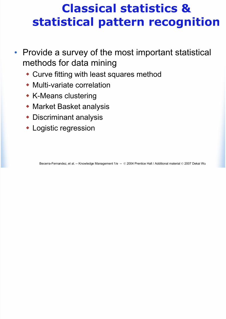
Classical statistics &statistical pattern recognition
• Provide a survey of the most important statistical
methods for data mining
Curve fitting with least squares method
Multi-variate correlation K-Means clustering
Market Basket analysis
Discriminant analysis Logistic regression

8/11/2019 KM Slides Ch12
http://slidepdf.com/reader/full/km-slides-ch12 7/48Becerra-Fernandez, et al. -- Knowledge Management 1/e -- © 2004 Prentice Hall / Additional material © 2007 Dekai Wu
Figure 12.14 – 2-D input dataplotted on a graph
x
y

8/11/2019 KM Slides Ch12
http://slidepdf.com/reader/full/km-slides-ch12 8/48Becerra-Fernandez, et al. -- Knowledge Management 1/e -- © 2004 Prentice Hall / Additional material © 2007 Dekai Wu
Figure 12.15 – data anddeviations
x
y
Best fitting
equation
x

8/11/2019 KM Slides Ch12
http://slidepdf.com/reader/full/km-slides-ch12 9/48Becerra-Fernandez, et al. -- Knowledge Management 1/e -- © 2004 Prentice Hall / Additional material © 2007 Dekai Wu
Induction of symbolic rules
• Present a detailed description of the symbolic approach
to data mining – rule induction by learning decision trees
• Present the main algorithm for rule induction
C5.0 and its ancestors, ID3 and CLS (from machine learning)
CART (Classification And Regression Trees) and CHAID, verysimilar algorithms for rule induction (independently developed in
statistics)
• Present several example applications of rule induction

8/11/2019 KM Slides Ch12
http://slidepdf.com/reader/full/km-slides-ch12 10/48
Becerra-Fernandez, et al. -- Knowledge Management 1/e -- © 2004 Prentice Hall / Additional material © 2007 Dekai Wu
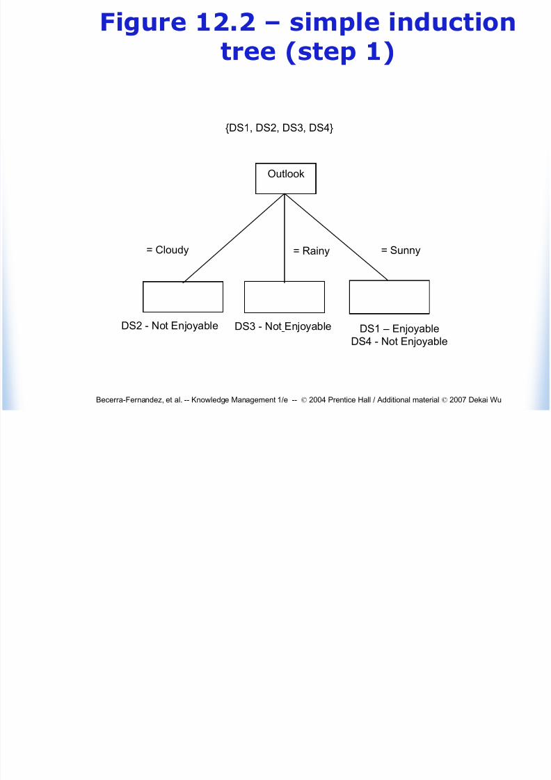
Table 12.1 – decision tables(if ordered, then decision lists)
Name Outlook Temperature Humidity Class
Data sample1 Sunny Mild Dry Enjoyable
Data sample2 Cloudy Cold Humid Not EnjoyableData sample3 Rainy Mild Humid Not EnjoyableData sample4 Sunny Hot Humid Not Enjoyable
Note: DS = Data Sample

8/11/2019 KM Slides Ch12
http://slidepdf.com/reader/full/km-slides-ch12 11/48
Becerra-Fernandez, et al. -- Knowledge Management 1/e -- © 2004 Prentice Hall / Additional material © 2007 Dekai Wu
Figure 12.1 – decision trees(a.k.a. classification trees)
Is the stock’s
price/earning
s ratio > 5?
Has the company’s
quarterly profit
increased over thelast year by 10% or
more?
Don’t
buy
NoYes
Root
node
Is the company’s
management
stable?
Leaf
node
Yes
Don’t
buy
No
Buy Don’t
Buy
Yes No

8/11/2019 KM Slides Ch12
http://slidepdf.com/reader/full/km-slides-ch12 12/48
Becerra-Fernandez, et al. -- Knowledge Management 1/e -- © 2004 Prentice Hall / Additional material © 2007 Dekai Wu
Induction trees
• An induction tree is a decision tree holding the
data samples (of the training set)
• Built progressively by gradually segregating the
data samples
8/11/2019 KM Slides Ch12
http://slidepdf.com/reader/full/km-slides-ch12 13/48
Becerra-Fernandez, et al. -- Knowledge Management 1/e -- © 2004 Prentice Hall / Additional material © 2007 Dekai Wu
Figure 12.2 – simple inductiontree (step 1)
DS3 - Not EnjoyableDS2 - Not Enjoyable
= Sunny= Cloudy = Rainy
RainRain
Outlook
{DS1, DS2, DS3, DS4}
DS1 – Enjoyable
DS4 - Not Enjoyable
Fi 12 3 i l

8/11/2019 KM Slides Ch12
http://slidepdf.com/reader/full/km-slides-ch12 14/48
Becerra-Fernandez, et al. -- Knowledge Management 1/e -- © 2004 Prentice Hall / Additional material © 2007 Dekai Wu
Figure 12.3 – simpleinduction tree (step 2)
None
DS3 - Not
Enjoyable
DS2 - Not
Enjoyable
= Sunny= Cloudy = Rain
RainRain
Outlook
Temperature DS1 – Enjoyable
DS4 – Not Enjoyable
= Cold = Hot= Mild
DS1 - Enjoyable DS4 – Not Enjoyable
{DS1, DS2, DS3, DS4}
8/11/2019 KM Slides Ch12
http://slidepdf.com/reader/full/km-slides-ch12 15/48
Becerra-Fernandez, et al. -- Knowledge Management 1/e -- © 2004 Prentice Hall / Additional material © 2007 Dekai Wu
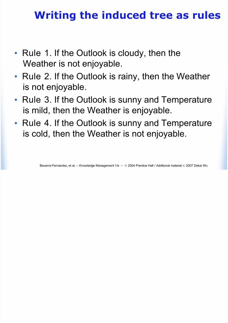
Writing the induced tree as rules
• Rule 1. If the Outlook is cloudy, then the
Weather is not enjoyable.
• Rule 2. If the Outlook is rainy, then the Weather
is not enjoyable.• Rule 3. If the Outlook is sunny and Temperature
is mild, then the Weather is enjoyable.
• Rule 4. If the Outlook is sunny and Temperatureis cold, then the Weather is not enjoyable.

8/11/2019 KM Slides Ch12
http://slidepdf.com/reader/full/km-slides-ch12 16/48
Becerra-Fernandez, et al. -- Knowledge Management 1/e -- © 2004 Prentice Hall / Additional material © 2007 Dekai Wu
Learning decision trees forclassification into multiple classes
• In the previous example, we were learning a function to predict a
boolean (enjoyable = true/false) output.• The same approach can be generalized to learn a function thatpredicts a class (when there are multiple predefinedclasses/categories).
• For example, suppose we are attempting to select a KBS shell for some application:
with the following as our options:
ThoughtGen, Offsite, Genie, SilverWorks, XS, MilliExpert
using the following attributes and range of values:
Development language: { Java, C++, Lisp }
Reasoning method: { forward, backward }
External interfaces: { dBase, spreadsheetXL, ASCII file, devices }
Cost: any positive number
Memory: any positive number
Table 12 2 –

8/11/2019 KM Slides Ch12
http://slidepdf.com/reader/full/km-slides-ch12 17/48
Becerra-Fernandez, et al. -- Knowledge Management 1/e -- © 2004 Prentice Hall / Additional material © 2007 Dekai Wu
Table 12.2 –collection of data samples (training set)
described as vectors of attributes (feature vectors)
Language Reasoningmethod
InterfaceMethod
Cost Memory Classification
Java Backward SpreadsheetXL 250 128MB MilliExpertJava Backward ASCII 250 128MB MilliExpert
Java Backward dBase 195 256MB ThoughtGenJava * Devices 985 512MB OffSiteC++ Forward * 6500 640MB GenieLISP Forward * 15000 5GB SilverworksC++ Backward * 395 256MB XS
LISP Backward * 395 256MB XS
Fi 12 4 d i i t lti f

8/11/2019 KM Slides Ch12
http://slidepdf.com/reader/full/km-slides-ch12 18/48
Becerra-Fernandez, et al. -- Knowledge Management 1/e -- © 2004 Prentice Hall / Additional material © 2007 Dekai Wu
Figure 12.4 – decision tree resulting fromselection of the language attribute
MilliExpert
ThoughtGen
OffSite
Language
Genie
XS
SilverWorks
XS
LispC++Java
i 2

8/11/2019 KM Slides Ch12
http://slidepdf.com/reader/full/km-slides-ch12 19/48
Becerra-Fernandez, et al. -- Knowledge Management 1/e -- © 2004 Prentice Hall / Additional material © 2007 Dekai Wu
Figure 12.5 – decision tree resulting from
addition of the reasoning method attribute
Language
MilliExpert
ThoughtGenOffSite
Backward
Forward Forward
Backward
C++Java
MilliExpertThoughtGen
OffSite
GenieXS
SilverWorksXS
Lisp
OffSite XS Ginie XS SilverWorks
Forward
Backwards
Figure 12 6 final decision

8/11/2019 KM Slides Ch12
http://slidepdf.com/reader/full/km-slides-ch12 20/48
Becerra-Fernandez, et al. -- Knowledge Management 1/e -- © 2004 Prentice Hall / Additional material © 2007 Dekai Wu
Figure 12.6 – final decisiontree
MilliExpert
ThoughtGen
OffSite
Backward
Forward Forward
Backward
C++Java
MilliExpert
ThoughtGen
OffSite
Language
Genie
XS
SilverWorks
XS
Lis p
OffSiteXS Genie XS SilverWorks
Forward
Backward
MilliExpert Mill iExper t ThoughtGen OffSite
SpreadsheetXL
ASCII Devices
dBase

8/11/2019 KM Slides Ch12
http://slidepdf.com/reader/full/km-slides-ch12 21/48
Becerra-Fernandez, et al. -- Knowledge Management 1/e -- © 2004 Prentice Hall / Additional material © 2007 Dekai Wu
Order of choosing attributes
• Note that the decision tree that is built depends
greatly on which attributes you choose first
Figure 12 2 simple induction

8/11/2019 KM Slides Ch12
http://slidepdf.com/reader/full/km-slides-ch12 22/48
Becerra-Fernandez, et al. -- Knowledge Management 1/e -- © 2004 Prentice Hall / Additional material © 2007 Dekai Wu
Figure 12.2 – simple inductiontree (step 1)
DS3 - Not EnjoyableDS2 - Not Enjoyable
= Sunny= Cloudy = Rainy
RainRain
Outlook
{DS1, DS2, DS3, DS4}
DS1 – Enjoyable
DS4 - Not Enjoyable
Figure 12 3 – simple

8/11/2019 KM Slides Ch12
http://slidepdf.com/reader/full/km-slides-ch12 23/48
Becerra-Fernandez, et al. -- Knowledge Management 1/e -- © 2004 Prentice Hall / Additional material © 2007 Dekai Wu
Figure 12.3 – simpleinduction tree (step 2)
None
DS3 - Not
Enjoyable
DS2 - Not
Enjoyable
= Sunny= Cloudy = Rain
RainRain
Outlook
Temperature DS1 – Enjoyable
DS4 – Not Enjoyable
= Cold = Hot= Mild
DS1 - Enjoyable DS4 – Not Enjoyable
{DS1, DS2, DS3, DS4}
Table 12 1 – decision tables

8/11/2019 KM Slides Ch12
http://slidepdf.com/reader/full/km-slides-ch12 24/48
Becerra-Fernandez, et al. -- Knowledge Management 1/e -- © 2004 Prentice Hall / Additional material © 2007 Dekai Wu
Table 12.1 – decision tables(if ordered, then decision lists)
Name Outlook Temperature Humidity Class
Data sample1 Sunny Mild Dry Enjoyable
Data sample2 Cloudy Cold Humid Not EnjoyableData sample3 Rainy Mild Humid Not EnjoyableData sample4 Sunny Hot Humid Not Enjoyable
Note: DS = Data Sample

8/11/2019 KM Slides Ch12
http://slidepdf.com/reader/full/km-slides-ch12 25/48
Becerra-Fernandez, et al. -- Knowledge Management 1/e -- © 2004 Prentice Hall / Additional material © 2007 Dekai Wu
Figure 12.7
= Dry= Humid
DS2 – Not Enjoyable
DS3 – Not Enjoyable
DS4 – Not Enjoyable
{DS1, DS2, DS3, DS4}
Humidity
DS1 - Enjoyable
Order of choosing attributes

8/11/2019 KM Slides Ch12
http://slidepdf.com/reader/full/km-slides-ch12 26/48
Becerra-Fernandez, et al. -- Knowledge Management 1/e -- © 2004 Prentice Hall / Additional material © 2007 Dekai Wu
Order of choosing attributes(cont)
• One sensible objective is to seek the minimal
tree, ie, the smallest tree required to classify alltraining set samples correctly Occam’s Razor principle: the simplest explanation is
the best• What order should you choose attributes in, so
as to obtain the minimal tree?
Often too complex to be feasible Heuristics used
Information gain, computed using information
theoretic quantities, is the best way in practice
ifi i l l k

8/11/2019 KM Slides Ch12
http://slidepdf.com/reader/full/km-slides-ch12 27/48
Becerra-Fernandez, et al. -- Knowledge Management 1/e -- © 2004 Prentice Hall / Additional material © 2007 Dekai Wu
Artificial Neural Networks
• Provide a detailed description of the connectionist
approach to data mining – neural networks
• Present the basic neural network architecture –
the multi-layer feed forward neural network• Present the main supervised learning algorithm –
backpropagation
• Present the main unsupervised neural networkarchitecture – the Kohonen network
Figure 12.8 – simple model of a

8/11/2019 KM Slides Ch12
http://slidepdf.com/reader/full/km-slides-ch12 28/48
Becerra-Fernandez, et al. -- Knowledge Management 1/e -- © 2004 Prentice Hall / Additional material © 2007 Dekai Wu
Figure 12.8 simple model of aneuron
x2
x1
xk
Activation
function
f()Inputs
y
W1
W2
Wn
Figure 12.9 – three common

8/11/2019 KM Slides Ch12
http://slidepdf.com/reader/full/km-slides-ch12 29/48
Becerra-Fernandez, et al. -- Knowledge Management 1/e -- © 2004 Prentice Hall / Additional material © 2007 Dekai Wu
Figure 12.9 three commonactivation functions
Threshold function Piece-wise
Linear functionSigmoid function
1.0
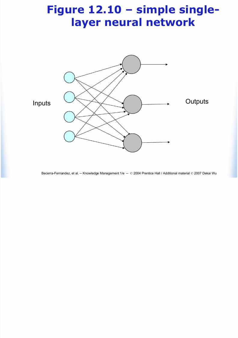
Figure 12.10 – simple single-
8/11/2019 KM Slides Ch12
http://slidepdf.com/reader/full/km-slides-ch12 30/48
Becerra-Fernandez, et al. -- Knowledge Management 1/e -- © 2004 Prentice Hall / Additional material © 2007 Dekai Wu
Figure 12.10 simple singlelayer neural network
Inputs Outputs
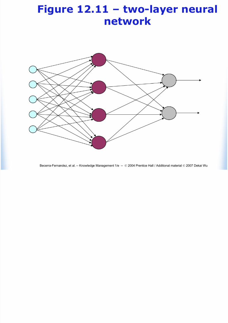
Figure 12.11 – two-layer neural
8/11/2019 KM Slides Ch12
http://slidepdf.com/reader/full/km-slides-ch12 31/48
Becerra-Fernandez, et al. -- Knowledge Management 1/e -- © 2004 Prentice Hall / Additional material © 2007 Dekai Wu
Figure 12.11 two layer neuralnetwork
Supervised Learning:

8/11/2019 KM Slides Ch12
http://slidepdf.com/reader/full/km-slides-ch12 32/48
Becerra-Fernandez, et al. -- Knowledge Management 1/e -- © 2004 Prentice Hall / Additional material © 2007 Dekai Wu
p gBack Propagation
• An iterative learning algorithm with three
phases:1. Presentation of the examples (input patterns with
outputs) and feed forward execution of the network
2. Calculation of the associated errors when the output
of the previous step is compared with the expected
output and back propagation of this error
3. Adjustment of the weights
Unsupervised Learning:
8/11/2019 KM Slides Ch12
http://slidepdf.com/reader/full/km-slides-ch12 33/48
Becerra-Fernandez, et al. -- Knowledge Management 1/e -- © 2004 Prentice Hall / Additional material © 2007 Dekai Wu
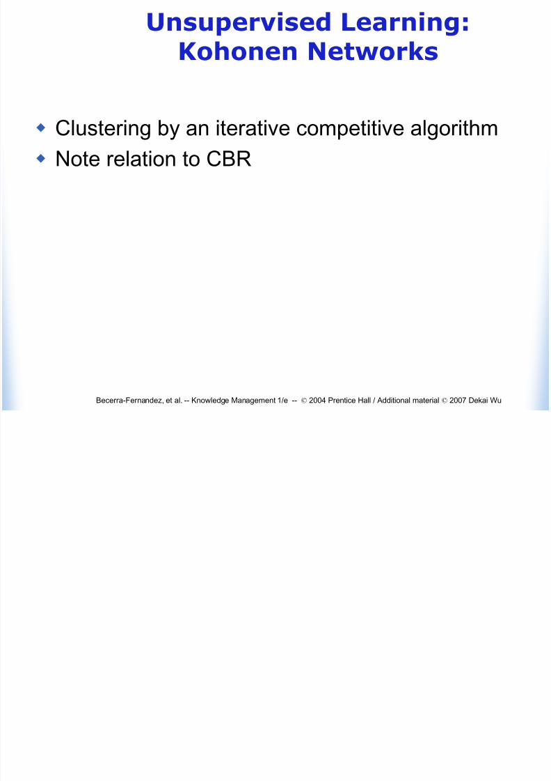
p gKohonen Networks
Clustering by an iterative competitive algorithm
Note relation to CBR
Figure 12.12 – clusters of

8/11/2019 KM Slides Ch12
http://slidepdf.com/reader/full/km-slides-ch12 34/48
Becerra-Fernandez, et al. -- Knowledge Management 1/e -- © 2004 Prentice Hall / Additional material © 2007 Dekai Wu
grelated data in 2-D space
Variable A
Variable B
Cluster #1
Cluster #2
Figure 12.13 – Kohonen self-

8/11/2019 KM Slides Ch12
http://slidepdf.com/reader/full/km-slides-ch12 35/48
Becerra-Fernandez, et al. -- Knowledge Management 1/e -- © 2004 Prentice Hall / Additional material © 2007 Dekai Wu
gorganizing map
Inputs
Wi
When to use what

8/11/2019 KM Slides Ch12
http://slidepdf.com/reader/full/km-slides-ch12 36/48
Becerra-Fernandez, et al. -- Knowledge Management 1/e -- © 2004 Prentice Hall / Additional material © 2007 Dekai Wu
When to use what
• Provide useful guidelines for determining what
technique to use for specific problems
Table 12 3

8/11/2019 KM Slides Ch12
http://slidepdf.com/reader/full/km-slides-ch12 37/48
Becerra-Fernandez, et al. -- Knowledge Management 1/e -- © 2004 Prentice Hall / Additional material © 2007 Dekai Wu
Table 12.3
Goal InputVariables
(Predictors)
OutputVariables
(Outcomes)
StatisticalTechnique
Examples
[SPSS, 2000]
Find linear combination of predictors thatbest separate thepopulation
Continuous Discrete Discriminant Analysis
• Predict instances of fraud• Predict whether customerswill remain or leave(churners or not)• Predict which customerswill respond to a newproduct or offer •Predict outcomes of various medical procedures
Predict theprobability of outcome being in
a particular category
Continuous Discrete Logistic andMultinomialRegression
• Predicting insurance policyrenewal• Predicting fraud
• Predicting which product acustomer will buy• Predicting that a product islikely to fail
Table 12 3 (cont )

8/11/2019 KM Slides Ch12
http://slidepdf.com/reader/full/km-slides-ch12 38/48
Becerra-Fernandez, et al. -- Knowledge Management 1/e -- © 2004 Prentice Hall / Additional material © 2007 Dekai Wu
Table 12.3 (cont.)
Output is a linear combination of input variables
Continuous Continuous Linear Regression
• Predict expected revenuein dollars from a newcustomer • Predict sales revenue for astore• Predict waiting time on hold
for callers to an 800 number.• Predict length of stay in ahospital based on patientcharacteristics and medicalcondition.
For experimentsand repeatedmeasures of the
same sample
Most inputsmust beDiscrete
Continuous Analysis of Variance(ANOVA)
• Predict whichenvironmental factors arelikely to cause cancer
To predict futureevents whosehistory has beencollected atregular intervals
Continuous Continuous Time Series Analysis
• Predict future sales datafrom past sales records
Goal InputVariables
(Predictors)
OutputVariables
(Outcomes)
StatisticalTechnique
Examples
[SPSS, 2000]
Table 12 4

8/11/2019 KM Slides Ch12
http://slidepdf.com/reader/full/km-slides-ch12 39/48
Becerra-Fernandez, et al. -- Knowledge Management 1/e -- © 2004 Prentice Hall / Additional material © 2007 Dekai Wu
Table 12.4
Goal Input(Predictor)Variables
Output(Outcome)Variables
StatisticalTechnique
Examples
[SPSS, 2000]
Predict outcomebased on valuesof nearestneighbors
Continuous,Discrete, and
Text
Continuous or Discrete
Memory-based
Reasoning(MBR)
•Predicting medicaloutcomes
Predict bysplitting data intosubgroups(branches)
Continuous or Discrete(Different
techniques usedbased on datacharacteristics)
Continuous or Discrete(Different
techniquesused based on
datacharacteristics)
DecisionTrees
•Predicting whichcustomers will leave•Predictinginstances of fraud
Predict outcomein complex non-linear environments
Continuous or Discrete
Continuous or Discrete
NeuralNetworks
•Predicting expectedrevenue•Predicting creditrisk
Table 12 5

8/11/2019 KM Slides Ch12
http://slidepdf.com/reader/full/km-slides-ch12 40/48
Becerra-Fernandez, et al. -- Knowledge Management 1/e -- © 2004 Prentice Hall / Additional material © 2007 Dekai Wu
Table 12.5
Goal Input(Predictor)Variables
Output(Outcome)Variables
StatisticalTechnique Examples [SPSS,2000]
Predict bysplitting data intomore than twosubgroups(branches)
Continuous,Discrete, or
Ordinal
Discrete Chi-square AutomaticInteraction Detection
(CHAID)
• Predict whichdemographiccombinations of predictors yield thehighest probability of
a sale• Predict whichfactors are causingproduct defects inmanufacturing
Predict bysplitting data intomore than two
subgroups(branches)
Continuous Discrete C5.0 • Predict which loancustomers areconsidered a “good”
risk• Predict whichfactors areassociated with acountry’s investmentrisk
Table 12 5 (cont )

8/11/2019 KM Slides Ch12
http://slidepdf.com/reader/full/km-slides-ch12 41/48
Becerra-Fernandez, et al. -- Knowledge Management 1/e -- © 2004 Prentice Hall / Additional material © 2007 Dekai Wu
Table 12.5 (cont.)
Predict bysplitting data intobinary subgroups(branches)
Continuous Continuous Classification andRegression Trees
(CART)
• Predict whichfactors areassociated with acountry’scompetitiveness• Discover whichvariables arepredictors of increased customer profitability
Predict by
splitting data intobinary subgroups(branches)
Continuous Discrete Quick, Unbiased,
Efficient, StatisticalTree (QUEST)
•Predict who needs
additional care after heart surgery
Goal Input(Predictor)Variables
Output(Outcome)Variables
StatisticalTechnique
Examples [SPSS,2000]
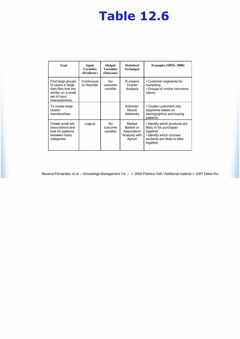
Table 12.6
8/11/2019 KM Slides Ch12
http://slidepdf.com/reader/full/km-slides-ch12 42/48
Becerra-Fernandez, et al. -- Knowledge Management 1/e -- © 2004 Prentice Hall / Additional material © 2007 Dekai Wu
Table 12.6
Goal InputVariables
(Predictor)
OutputVariables
(Outcome)
StatisticalTechnique
Examples [SPSS, 2000]
Find large groupsof cases in largedata files that aresimilar on a small
set of inputcharacteristics,
Continuousor Discrete
Nooutcomevariable
K-meansCluster
Analysis
• Customer segments for marketing• Groups of similar insuranceclaims
To create largecluster memberships
KohonenNeural
Networks
• Cluster customers intosegments based ondemographics and buyingpatterns
Create small set
associations andlook for patternsbetween manycategories
Logical No
outcomevariable
Market
Basket or Association
Analysis with Apriori
• Identify which products are
likely to be purchasedtogether • Identify which coursesstudents are likely to taketogether
Errors andh i i ifi i DM

8/11/2019 KM Slides Ch12
http://slidepdf.com/reader/full/km-slides-ch12 43/48
Becerra-Fernandez, et al. -- Knowledge Management 1/e -- © 2004 Prentice Hall / Additional material © 2007 Dekai Wu
their significance in DM
• Discuss the importance of errors in data mining
studies• Define the types of errors possible in data
mining studies
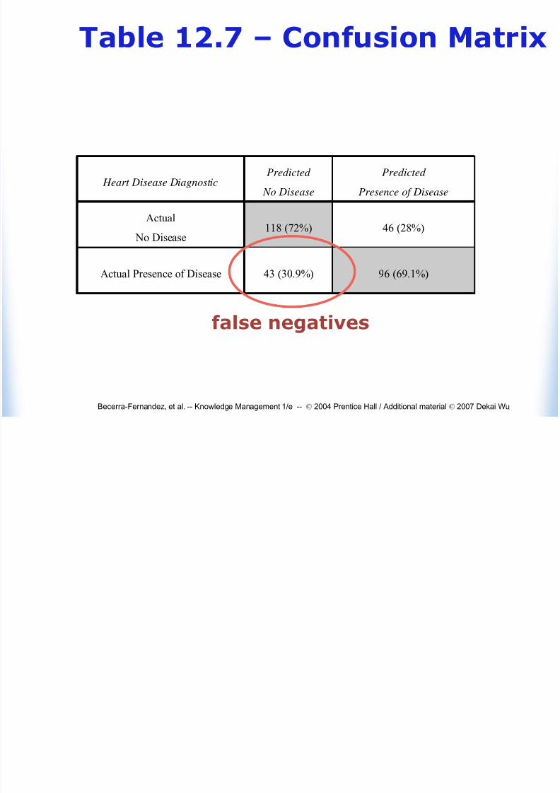
Table 12.7 – Confusion Matrix

8/11/2019 KM Slides Ch12
http://slidepdf.com/reader/full/km-slides-ch12 44/48
Becerra-Fernandez, et al. -- Knowledge Management 1/e -- © 2004 Prentice Hall / Additional material © 2007 Dekai Wu
Table 12.7 Confusion Matrix
Heart Disease DiagnosticPredicted
No Disease
Predicted
Presence of Disease
Actual
No Disease118 (72%) 46 (28%)
Actual Presence of Disease 43 (30.9%) 96 (69.1%)
Table 12.7 – Confusion Matrix
8/11/2019 KM Slides Ch12
http://slidepdf.com/reader/full/km-slides-ch12 45/48
Becerra-Fernandez, et al. -- Knowledge Management 1/e -- © 2004 Prentice Hall / Additional material © 2007 Dekai Wu
Table 12.7 Confusion Matrix
Heart Disease DiagnosticPredicted
No Disease
Predicted
Presence of Disease
Actual
No Disease118 (72%) 46 (28%)
Actual Presence of Disease 43 (30.9%) 96 (69.1%)
false negatives
Table 12.7 – Confusion Matrix

8/11/2019 KM Slides Ch12
http://slidepdf.com/reader/full/km-slides-ch12 46/48
Becerra-Fernandez, et al. -- Knowledge Management 1/e -- © 2004 Prentice Hall / Additional material © 2007 Dekai Wu
Table 12.7 Confusion Matrix
Heart Disease DiagnosticPredicted
No Disease
Predicted
Presence of Disease
Actual
No Disease118 (72%) 46 (28%)
Actual Presence of Disease 43 (30.9%) 96 (69.1%)
false positives
Conclusions

8/11/2019 KM Slides Ch12
http://slidepdf.com/reader/full/km-slides-ch12 47/48
Becerra-Fernandez, et al. -- Knowledge Management 1/e -- © 2004 Prentice Hall / Additional material © 2007 Dekai Wu
Co c us o s
• You should know when to use:
Curve-fitting algorithms.
Statistical methods for clustering.
The C5.0 algorithm to capture rules from examples.
Basic feedforward neural networks with supervised
learning.
Unsupervised learning, clustering techniques and the
Kohonen networks.
Other statistical techniques.

8/11/2019 KM Slides Ch12
http://slidepdf.com/reader/full/km-slides-ch12 48/48
Becerra-Fernandez, et al. -- Knowledge
Management 1/e -- © 2004 Prentice Hall
Additional material © 2007 Dekai Wu
Chapter 12
Discovering New Knowledge –
Data Mining
Recommended