Kent Academic RepositoryFull text document (pdf)
Copyright & reuse
Content in the Kent Academic Repository is made available for research purposes. Unless otherwise stated all
content is protected by copyright and in the absence of an open licence (eg Creative Commons), permissions
for further reuse of content should be sought from the publisher, author or other copyright holder.
Versions of research
The version in the Kent Academic Repository may differ from the final published version.
Users are advised to check http://kar.kent.ac.uk for the status of the paper. Users should always cite the
published version of record.
Enquiries
For any further enquiries regarding the licence status of this document, please contact:
If you believe this document infringes copyright then please contact the KAR admin team with the take-down
information provided at http://kar.kent.ac.uk/contact.html
Citation for published version
Degl’Innocenti, Marta and Matousek, Roman and Sevic, Zeljko and Tzeremes, Nickolaos (2017)Bank efficiency and financial centres: Does geographical location matter? Journal of InternationalFinancial Markets, Institutions and Money, 46 . pp. 188-198. ISSN 1042-4431.
DOI
https://doi.org/10.1016/j.intfin.2016.10.002
Link to record in KAR
http://kar.kent.ac.uk/60225/
Document Version
Author's Accepted Manuscript
1
Bank Efficiency and Financial Centres: Does Geographical Location Matter?
Marta Degl’Innocenti1, Roman Matousek2*, Zeljko Sevic3, Nickolaos G. Tzeremes4
1 University of Southampton, Southampton Business School, Highfield, Southampton, SO17 1BJ, United Kingdom. Tel. +44 23 8059 8093, Fax +44 23 8059 3844, E-mail address: [email protected]. 2* Corresponding Author: University of Kent, Kent Business School, Canterbury, Kent, CT2 7NZ, United Kingdom, Tel. +44 (0)1227 82 7465, Fax 44 (0)1227 8271111, E-mail address: [email protected]. 3 The Universiti Utara Malaysia, Othman Yeop Abdullah Graduate School of Business, 06010UUM Sintok, Kedah Darul Aman, Maslaysia, [email protected] 4 University of Thessaly, Department of Economics, Korai 43, 38333, Volos, Greece, Tel. +30 2421 074911, Fax +30 2421074772, E-mail address: [email protected].
Abstract
This paper examines the relationship between bank performance and geographical location with respect to the two major global financial centres, New York and London. It provides new insights on the spatial effects of the 2008-2009 Global Financial Crisis (GFC) on the technical efficiency of the top-1000, world-leading banks in terms of total assets. The results reveal that the distance of banks’ headquarters to these financial centres matters. In particular, banks that are located at a bigger distance from New York and London present a lower technical efficiency than banks that are closer to these financial centres. In addition, the results show that the Global Financial Crisis has magnified the effect of distance and the need for banks to be closer to global financial centres during the ‘core’ of that period.
Keywords: Bank performance; Financial centres; Conditional efficiency; Robust estimators.
2
1. Introduction
London and New York have historically played an important role as global financial
centres within the financial markets and have influenced the formation of the
worldwide financial architecture. French et al. (2009) argue that these two financial
centres have not been only a catalyst for changes in terms of financial globalization
but also in generating the conditions that have led to the Global Financial Crisis
(GFC) in 2007-2008 that have spillovered to other countries around the world.
Engelen and Grote (2009) express a similar view, noting that the importance of these
financial centres was particularly reinforced during the GFC.
The interconnectivity between New York and London and their impact on the
global financial markets cannot be compared to any other cities like, for example,
Tokyo (see for a comprehensive discussion Wójcik 2013). Cassis (2010) and Wójcik
(2013) justify the unique position and importance of London and New York, as
financial centres, due to historical complementarities and affinity in terms of the
cultural geographies of finance1 but also due to factors like global trade, financial
imbalances with exporter’s countries, financial deregulation, and the implementation
of the newest technologies.
Despite the relevance of the New York-London axis in the context of the
global financial markets, so far it is still unclear how and to what extent proximity to
these two financial centres matters for international bank efficiency.
Various empirical studies specifically examine the different forms of bank
efficiency, such as, cost, profit, technical and allocative efficiency across different
regions and continents (recently, Assaf et al. 2013; Tzeremes 2014). However, these
1 Media companies are mainly located in global financial centres and they played a significant role in generating hotspots of irrational exuberance in the housing market (Wójcik, 2013).
3
studies only analyse the bank efficiency in isolated countries or provide a comparative
analysis without taking into account the geographical location of banks2.
The lack of this latter type of research is due to the fact that economic and
geographical literature (eg. Storper and Venables 2004; Boschma and Weterings
2005) unambiguously provides anecdotal evidence that the proximity to
agglomeration and co-location can boost firm productivity, competition, development
of specialized labour pool, knowledge spillover, diffusion of innovation. Following
the new economic geography (NEG), this paper draws attention to the wider
economic-geographic relations across space and time of the technical efficiency in the
banking industry, and uncovers how and to what extent inefficiencies have been
transmitted to the banking system worldwide from the New York-London axis. The
imposed research question is further supported by empirical research that shows that
geographical location remains important for business performance in general
(recently, McCauley et al. 2012), and one cannot observe the ‘end of geography’
despite new technological advantage and new means of communication and
information transfer.
Throughout the paper we will show that the current GFC is an optimal
laboratory to explore how the geographical location, in particular the proximity
(distance) from these two financial centres, affects performance of large international
banks. Differently from previous studies on the contagion effect during the GFC (e.g.
Eichengreen et al. 1996; Glick and Rose 1999; Ali and Lebreton 2007), the paper
contributes to a nuanced understanding of the spatial processes that embedded banks
into global markets though global financial centres. Specifically, drawing on the new
economic geography approach and spatial selection model proposed by Baldwin and
2 There are a few exceptions, such as Berger and DeYoung (2001), Berger and DeYoung (2006), Deng and Elyasiani (2008).
4
Okubo (2006), we ascertain that global financial markets attract a high number of
banks that are however the most efficient. In particular, the spatial selection model
and the new economic geography framework assists us to examine how and to what
extent the bank distance from New York-London axis changes bank efficiency.
To our best knowledge, this is the first paper that attempts to examine the
relationship between a bank’s performance and geographical location with respect to
global financial centres. Moreover, it provides new insights on the spatial effect of the
GFC on bank technical efficiency. We use a sample of the top 1000 world leading
banks measured in terms of total assets. These banks are more interconnected to each
other in the global financial market and subsequently more subject to the effect of
global financial centres and economic dynamics than their smaller counterparts. They,
therefore, suit the scope of this paper better.
From a methodological viewpoint, we introduce a new non-parametric
estimation technique to calculate the technical efficiency of banks.3 Our model is
based on the latest developments of the probabilistic approach of efficiency
measurement (B<din et al. 2012). The advantage of this method is that the
probabilistic approach does not impose a separability assumption. Therefore the
exogenous variables (i.e. the distance from headquarters4) directly influence the shape
of the frontier (i.e., a separability condition is not assumed). As a result, the obtained
efficiency estimates are determined by the inputs, outputs and the exogenous variable
(for details see Simar and Wilson 2011).
We organize the rest of the paper as follows: Section 2 reviews the literature;
Section 3 discusses the data sample and the variables used in our empirical analysis; 3For recent applications of the latest advances of nonparametric frontier analysis on the banking sector see the studies by Fukuyama and Matousek, (2011), Tsionas et al. (2015), Tzeremes (2015), Matousek and Tzeremes (2016), Salim et al. (2016) and Wanke et al. (2016). 4We calculated the distance of the headquarters to New York and London by using longitude and latitude coordinates.
5
Section 4 describes the model and method of estimation. Section 5 the empirical
results, and Section 6 summarizes our findings and sets out our conclusions.
2. Literature Review
Despite the growth of powerful global financial centres during the financialisation era
(Stockhammer 2008), research studies have neglected to investigate the
interconnectedness between finance and economic geography.
Whilst several papers have focused on geography and efficiency, as well as
the performance of banks (e.g. Berger and De Young 1997; Deng and Elyasiani 2008;
Mc Cauley et al. 2012), and geographical distance and the activities of financial
intermediaries (e.g. Degryse and Ongena 2005; Carey and Nini 2007), so far no one
has explored the effect of the distance of a bank’s headquartes from global financial
centres on bank efficiency. To come to a better understanding of the effects of
financial centres on the efficiency of banks in a global economic system, we make use
of the NEG approach which focuses on the development of economic agglomeration,
but which has so far has not been systematically applied in the context of global
financial centres (Grote, 2008). Engelen and Grote (2009) maintain that NEG
considers financial centres to be the net sum of centripetal and centrifugal forces
where rational agents pursue ‘satisficing’ strategies (Simon 1982). Specifically, they
explain that these centripetal forces are the “effects of dedicated infrastructure, firms
using each other’s output as input, specialised labour markets, and knowledge
spillovers”; while centrifugal forces are “conceptualised as increasing transportation
costs, increasing rents and negative technological effects” (Engelen and Grote 2009,
p. 689). The NEG models predict the process of accumulation of firms in specific
locations. As argued by Krugman (1998), NEG focuses on the linkages that foster
6
geographical concentration, and these “linkages, which are mediated by transportation
costs, are naturally tied to distance” (p.9). In the banking sector geographic proximity
to clients represents an important competitive advantage, especially when transaction
costs, such as transportation and information costs exist and are non-negligible (e.g.
Dell’Ariccia 2001). Physical proximity to other firms is needed to collect information
about local economic conditions and customers in the financial markets (Thrift 1994).
However, recent technological innovations and communication technologies have
facilitated the transmission of information across large distances (Cerqueiro et al.
2009), and may have altered the effects of financial centres in terms of both the
concentration of activities and increasing mobility (O’Brien 1992).
Relaxing the assumption of homogeneity of firm-level productivity, Baldwin
and Okubo (2006) demonstrate that big markets attract a high number of firms
overall, but they also attract the most efficient firms. In line with the spatial selection
model proposed by Baldwin and Okubo (2006), we maintain that the most efficient
banks are located close to the global financial centres. Therefore, we expect that as the
distance from the headquarters of commercial banks to the New York-London axis, as
well as the transaction costs, increases, the level of efficiency of those banks declines.
The agglomeration forces lead to a concentration of firms in a location in a context of
increasing returns, economies of scales and imperfect competition, which can enhance
the efficiency of banks (Krugman 1991).
Finally, we also investigate how and to what extent the effect of the 2008-
2009 Global Financial Crisis has spread out to banks through the enhancement of
their cost inefficiencies. As argued by Wainwright (2012), more studies on the space
and scale of the Global Financial Crisis have begun to emerge that underline the
spatial dynamics of the crisis in different specific economic, social and political
7
geographical settings. However, the existing literature on finance and space is still
scarce, even though it can enhance our comprehension of the origin and aftermath of
the crisis (see for example Martin 2010; Wainwright 2012). As concerns our analysis,
we expect an intensification of the negative effect of distance from the headquarters
of commercial banks to the new York-London axis during and after the 2008-2009
Global Financial Crisis, mainly driven by an increase in transaction costs. After
October 2008, the confidence of investors in the banking system has dropped since
banks were perceived as opaque entities and even the interbank lending market
‘‘froze’’ because of the increasing uncertainty about counterparty solvency (e.g.
Pritsker 2010; Flannery et al. 2013).
3. Data and Variables
We collected our sample of the top-1000 commercial banks around the world
using unconsolidated balance sheets from the Bureau van Dijk’s Bankscope database.
The sample is balanced and includes the top multinational banks which have their
headquarters in 80 countries. The data Longitude and latitude coordinates were used
to calculate the google map distance between bank headquarters and the financial
centres of New York and London. The analysed period spans from 2004 to 2010.
In the banking literature, there has been an extensive discussion of how to
model bank production processes. Berger and Humphrey (1992) highlight that there
are several approaches that can be used to model the bank production process: the
production approach; the user-cost approach; the value added approach; and the dual
approach. The standard methods applied in banking are the intermediation and
production approaches. Under the intermediation approach, banks use purchased
funds together with physical inputs to produce various assets (measured by their
8
value). The production approach assumes that banks use only physical inputs, such as
labour and capital, to produce deposits and various assets (measured by the number of
deposit and loan accounts at a bank, or by the number of transactions for each
product). We adopt the intermediation approach to model bank production and
consider banks to be intermediaries of financial services that purchase inputs in order
to generate earning assets (Sealey and Lindley 1977). Berger and Humphrey (1997)
suggest that the intermediation approach is best suited for evaluating bank efficiency,
whereas the production approach is appropriate for evaluating the efficiency of bank
branches.
Furthermore, we apply a nonparametric robust frontier analysis in order to
measure banks’ efficiency levels which does not put any restrictions on the functional
form of the relationships between inputs and outputs used. According to Holod and
Lewis (2011, p.2802) nonparametric approaches are very appealing for estimating the
efficiency of financial institutions that do not have a well-defined production function.
In our modelling setting we use three inputs and three outputs for the time period
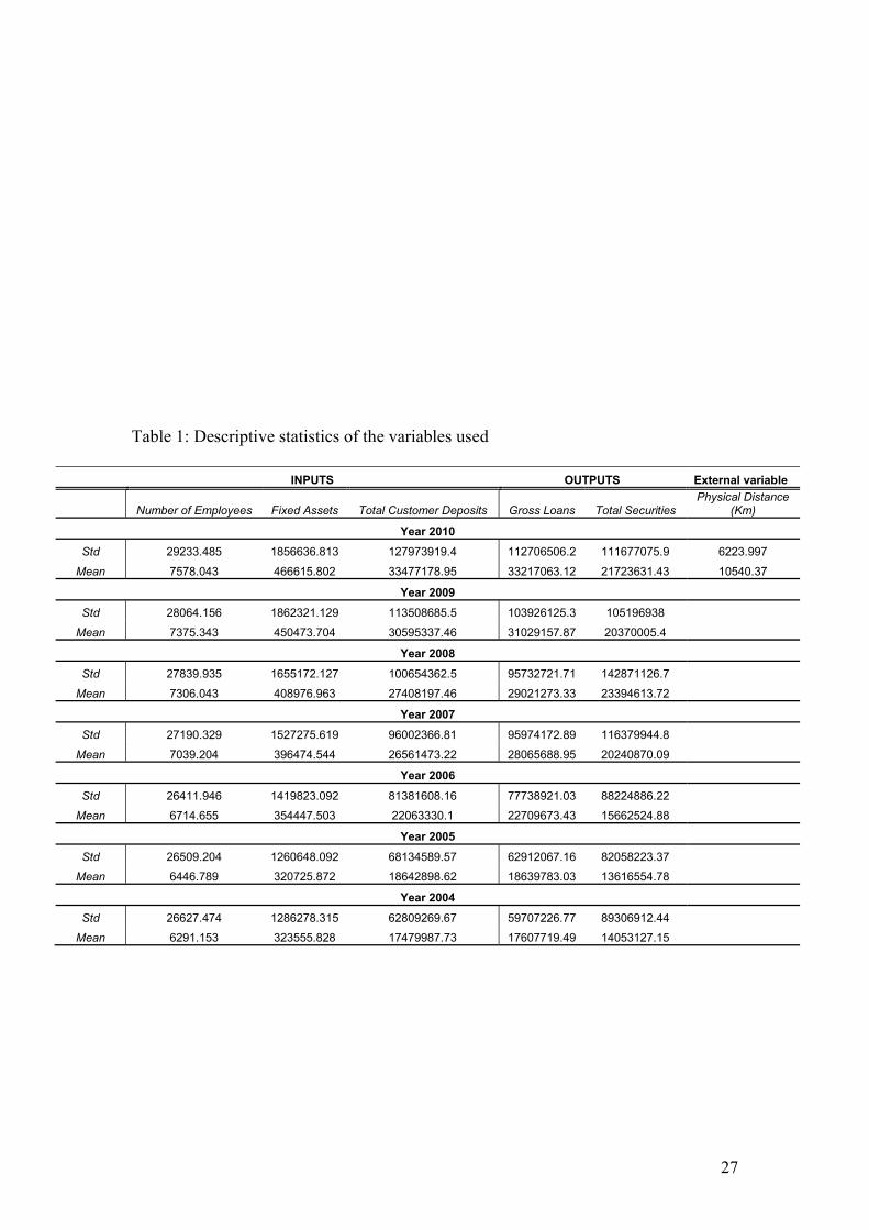
2004-2010 for data derived from the BankScope database. Table 1 provides the
descriptive statistics of the variables used. We use number of employees, total
customer deposits5 and fixed assets (in thousands US dollars) as inputs and gross
loans and total securities as outputs (in thousands US dollars). As an external variable
( z ) we use the summation of the distance in kilometres between the city in which the
5According to Holod and Lewis (2011) the treatment of deposits as input or as output in the bank
production process has raised a considerable debate amongst scholars. Several studies (Berger et al.
1987; Hunter & Timme 1995; Berger and DeYoung 1997; Devaney and Weber 2002) treat deposits as
an output in bank production process since banks provide customers value-added outputs in the form of
clearing, record-keeping, and security services, and hence they accept deposits.
9
bank has its headquarters and the two main financial centres of New York and
London.6
According to Daraio and Simar (2007, pp. 78) the application of full
nonparametric models (DEA-Data Envelopment Analysis and FDH-Free Disposal
Hull) can suffer from different problems, such as extreme values/outliers (which
provide them with the property of a deterministic nature) and the curse of
dimensionality. Therefore, in order to avoid those problems, we apply partial
nonparametric frontiers (order-m) introduced by Cazals et al. (2002), which will
enable us to avoid the main problems when using full nonparametric frontiers and
thus to obtain robust results.
Table 1 about here
4. Methodology
To calculate technical efficiency we employed the probabilistic approach of efficiency
measurement introduced by Daraio and Simar (2005, 2007) and the latest
developments by B<din et al. (2012). Then we compare the unconditional and
conditional efficiency scores by applying the nonparametric test for equality of
distributions (Li et al., 2009). According to Black and Smith (2004) and Frölich
(2008) the main advantage of the nonparametric method is the fact that it overcomes
problems associated with endogenous control variables and omitted variables, and it
is consistent when instrumental variables are excluded from the model. In fact, a
nonparametric model compares only observations having the same/similar values for
the control variable, whereas the parametric regression combines all observations in a 6 For instance the headquarters of National Bank of Abu Dhabi is 11025 kilometres from New York
and 5476 kilometres from London. Therefore our distance factor ( z ) is equal to 16501 kilometres (i.e.
National Bank of Abu Dhabi distance to New York distance to London11025 5476 z ).
10
unified regression framework. Therefore, the adopted nonparametric framework
provides us with the advantage to focus only on the direct effect of distance on bank
efficiency excluding any additional variables.
Following Daraio and Simar (2005), a bank’s production technology can be
characterized by a set of inputs px R which can produce a set of outputs qy R .
Formally banks’ production processes can be defined as:
, can produce y .p qx y R x (1)
Then the Farrell measure of input-oriented efficiency score can be defined as:
( , ) inf ( , ) .x y x y (2)
Next the production process can be described by the joint probability measure of (X,Y)
on qp xRR . Then, the knowledge of the probability function (.,.)XYH can be defined
as:
( , ) Prob( , )XYH x y X x Y y (3)
For the input oriented case the efficiency scores ),( yx for ),( yx can be
defined as:
( , ) inf ( ) 0 inf ( , ) 0 .X Y X Yx y F x y H x y (4)
Following Cazals et al. (2002) for an input orientation the order-m frontier can
be introduced as follows. Having a fixed integer 1m for a given level of output y
we obtain the random production set of the order-m units producing more than y as:
miyyXxRyxy iqp
m ,...,1,,)( ',
' (5)
In addition for any x we can define ~
( , ) inf ( , ) ( ) ,m mx y x y y (6)
11
and banks’ order-m efficiency scores can be defined as:
~
, , ( , ) .m n mx y E x y Y y
(7)
Daraio and Simar (2007) show that the order-m efficiency score is the
expectation of the input efficiency score of a bank yx, when compared to m (in our
case 10)7 banks randomly drawn from the population of banks producing more
outputs than the level y. The efficiency scores computed under the order-m
formulation can take values greater than one. When the estimator has a value greater
than one it indicates that the bank operating at the level yx, is more efficient than
the average of m peers. In an input oriented case where a bank has an efficiency score
of 0.7, it means that the bank uses 30% more inputs than the expected value of the
minimum input level of m other banks drawn from the population of banks producing
a level of output y . Finally, when m then yxyx FDHnm ,,,
.
Following Daraio and Simar (2005), we assume that different variables
(exogenous to the production process) r can be used to explain the efficiency
variations of the production process. In contrast to the traditional two-stage
approaches, the probabilistic approach does not impose a separability assumption
between Z values and the input-output space (Simar and Wilson, 2011). As described
previously, the exogenous variable used in this study is the sum of the kilometric
distance between the banks’ head office and the two financial centres (i.e New York
and London). The idea is to condition the banks’ production process to a given value
of kilometre distance zZ . The joint distribution YX , conditional on zZ defines
the production process if zZ as:
7For larger values of m the results converge very quickly to the free disposal assumption-FDH
efficiency scores (Deprins et al. 1984).
12
( , ) Prob( , ).XY ZH x y z X x Y y Z z (8)
Then bank’s input-oriented technical efficiency scores under the effect of the external
factor can be obtained as:
,( , ) inf ( , ) 0 .X Y Zx y z F x y z (9)
Thus the conditional order-m nonparametric estimator8 can be obtained as:
,( , ) ( ( , ) , ).z
X Y Zm mx y z E x y y z
(10)
By following, B<din et al. (2012) the global influence of Z (i.e. the distance
from the two financial centres) on banks’ production process can be obtained by
comparing the conditional order-m frontier (equation 10) to their unconditional
equivalents (equation 7). In a univariate case of Z a scatter-plot of the ratios zQ 9
against Z and its smoothed nonparametric regression line would indicate the global
effect of Z on the production process. If the smoothed nonparametric regression
increases it indicates that Z is unfavourable to banks’ performance levels. When the
regression decreases then is favourable10.
5. Empirical Results
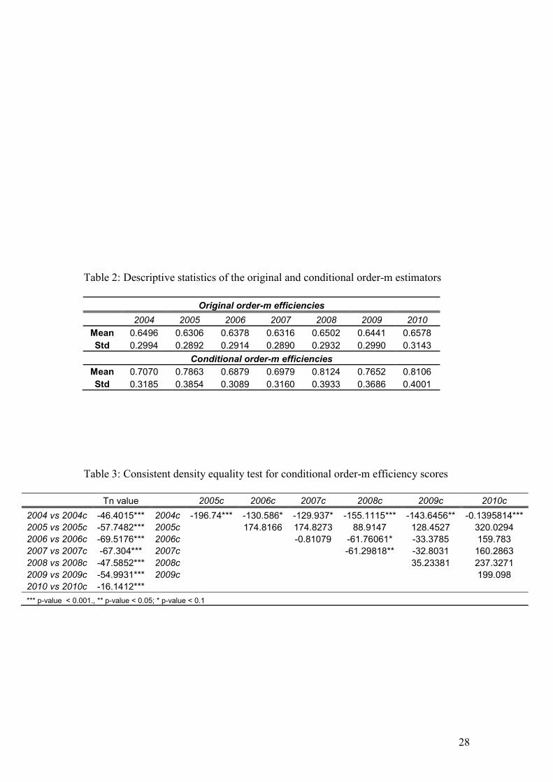
In Table 2, we provide the descriptive statistics of the original efficiency
scores and the conditional efficiency scores to distance from the two financial centres.
We observe that the mean values of bank efficiency, without including the distance
8For the calculation of the conditional efficiency estimates some smoothing and estimation of the appropriate bandwidths is required. This can be obtained by following the least-squares cross-validation criterion-LSCV (Hall et al. 2004; Li and Racine,2004) based procedure introduced by B<din et al. (2010). For the linear programs required to calculate the conditional estimates, see Daraio and Simar (2005, 2007). 9 This can be defined as: , ,( , ) / ( , )m n m nzQ x y z x y
. 10In order to have a visualisation of the effect we apply the nonparametric regression estimator introduced by Nadaraya (1964) and Watson (1964) and we use the LSCV criterion for bandwidth selection.
13
factor, are relatively stable over the analysed period. We report the efficiency levels
through the period are on average terms between 0.63 – 0.65. That means that on
average terms, the efficiency levels of the largest multinational banks remain
relatively unchanged over 2004 to 2010. That corresponds with the estimated standard
deviation values. Standard deviations range from 0.29 to 0.31. However, if the
distance is added into the model the results as has been expected change. These
results indicate that the distance is an important variable in measuring bank
efficiency.
Table 2 about here
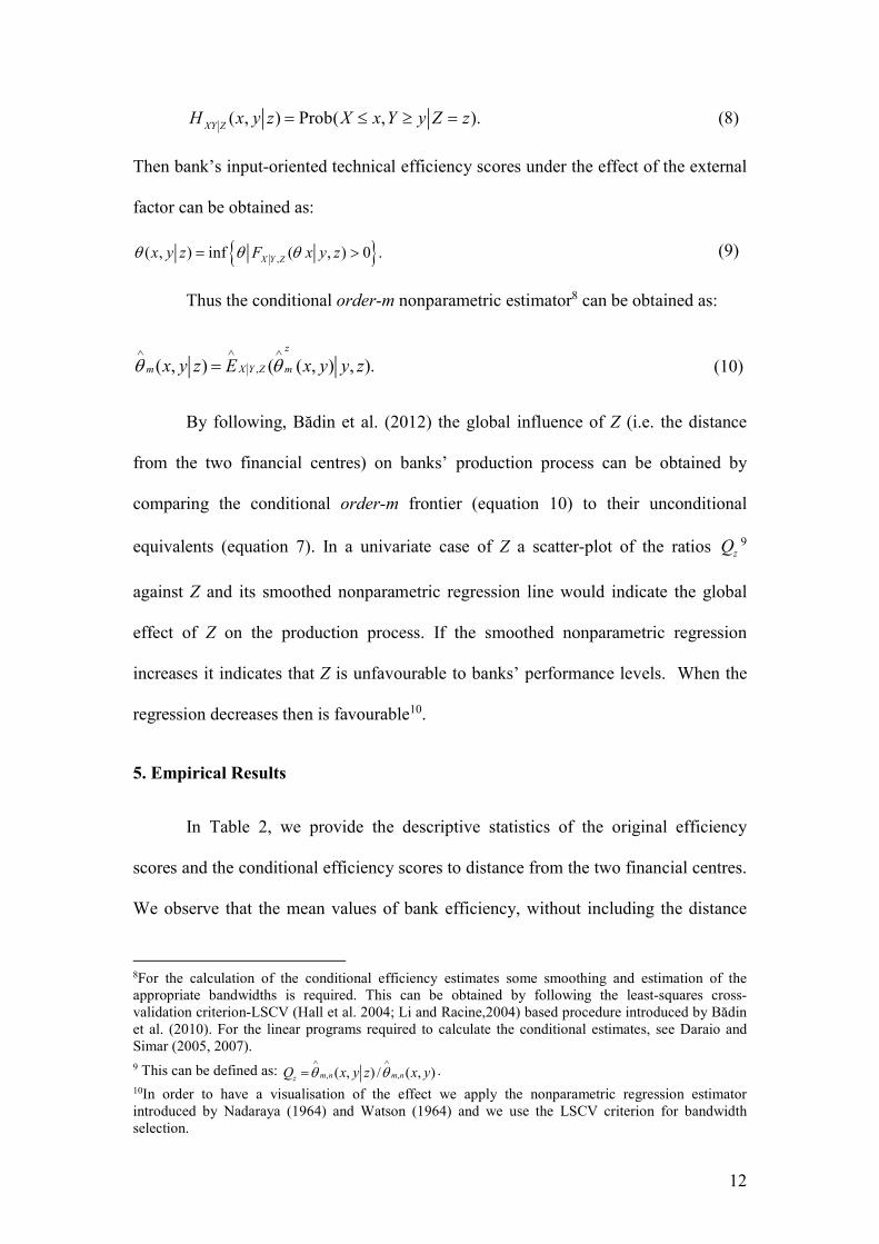
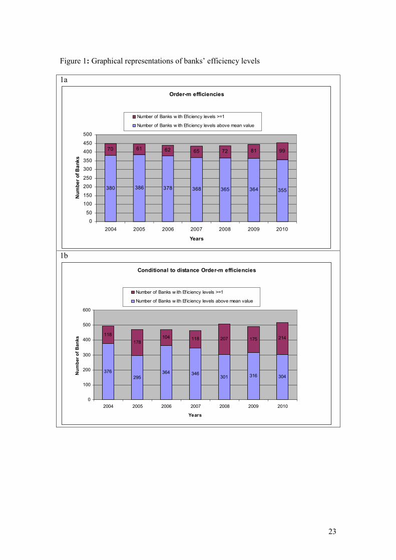
This is further supported by our results that we present in Figure 1. We split
the banks into two groups; those with the efficiency scores higher or equal to one, and
those with efficiency scores higher than the mean efficiency score. The higher the
score the more efficient banks are over the examined period for conditional and
unconditional measures. Figure 1a lists the bank efficiency scores when we are not
taking into account the effect of distance from the two financial centres (sub figure
1a). It can be viewed that we have (on average terms) 72 banks that appear to be
efficient over the examined period. Focusing more on the original estimates
(subfigure 1a) we realise that after the Global Financial Crisis of 2008 the number of
efficient banks started to increase from 65 (in 2007) to 99 (in 2010). Subfigure 1a
indicates the number of banks with efficiency values above average (this number
includes also the banks with efficiency scores 1 ). In contrast with our previous
finding the number of banks having an efficiency score above samples’ average value
tends to decrease over the years (from 380 for 2004, to 355 for 2010).
Furthermore, subfigure 1b indicates banks’ efficiency levels when taking into
account the effect of the distance from banks’ headquarters and the two financial
14
centres. When the Global Financial Crisis started in 2007, our findings suggest that
346 banks had efficiency scores above the samples average efficiency score (0.6979).
This number decreased in 2008, 2009 and 2010. This indicates that the distance
between banks’ headquarters and the two financial centres affected banks’ overall
efficiency levels over the period of the crisis. In contrast, subfigure 1b indicates that
after the initiation of Global Financial Crisis the number of banks with efficiency
scores 1 has increased from 118 (in 2007) to 214 (in 2010) indicating a possible
divergence of banks’ performance having an efficiency value above average, which is
attributed to the distance effect.
Figure 1 about here
Next, we test whether distance has a significant influence on banks’ efficiency levels.
In doing so, we apply the nonparametric test for equality of distributions (Li et al.,
2009) between the obtained efficiency scores. In Table 3, we show the results
obtained from the applied equality test. The first column lists the results for equality
between the unconditional (2004) and conditional (2004c) banks’ efficiency scores for
the year 2004. Our test statistic is -46.4015 with a p-value <0.001. Based on this
result, we have to reject the null hypothesis of equality of distribution and we accept
that they are not equal. Therefore, in this particular case, the results indicate that
distance has an effect on banks’ efficiency levels since the distributions of efficiency
measures (both conditional and unconditional) for that year are not the same.
Our findings suggest that we have to reject the null hypothesis of equality of
the distributions of the obtained efficiencies (between the unconditional and
conditional efficiency scores) for all the years of our analysis, indicating clearly that
the distance between bank headquarters and the two financial centres influences
banks’ performance. Furthermore, we test the equality of distributions among the
15
conditional efficiency scores over the years. We may accept the null hypothesis in
several cases. This finding suggest equality of the distributions of banks’ conditional
efficiency scores between different years.
Table 3 about here
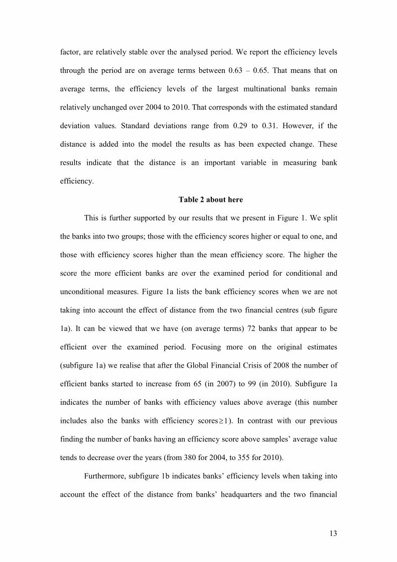
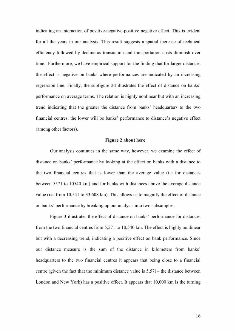
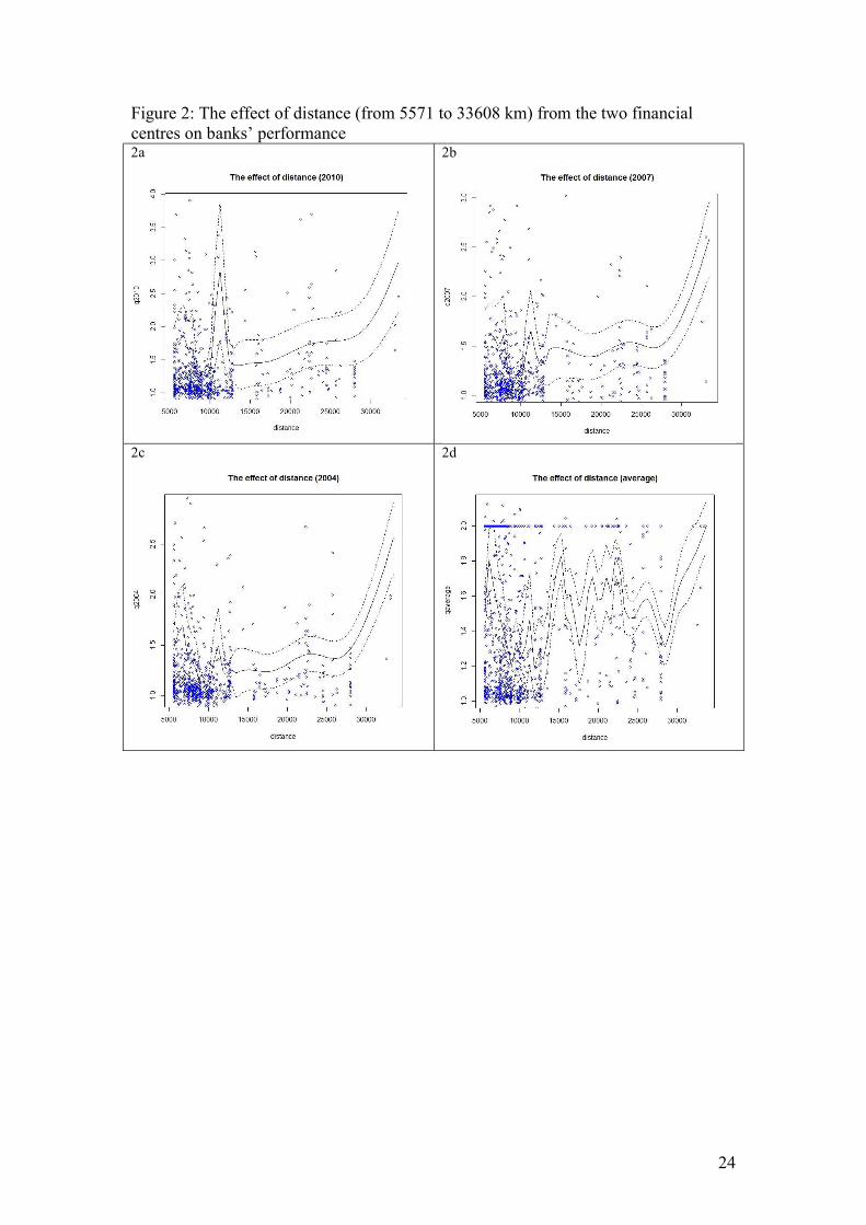
Next, we provide evidence that distance from the two financial centres
influences banks’ efficiency over the years and in what way this influence is
attributed to banks’ performance. We use the methodology of the visualisation effect
on the influence of distance based on several authors (Daraio and Simar 2005, 2007;
B<din et al. 2012). Figure 2 illustrates several smoothed nonparametric regression
lines of the effect of distance on the ratio of conditional to unconditional efficiency
scores for every year. As we explained before, if the smoothed nonparametric
regression line is increasing it indicates that the distance from the banks’ headquarters
to the two financial centres is detrimental to banks’ efficiency levels acting as an
‘extra’ undesirable output. By contrast, if the regression line is decreasing then it
specifies that distance is conductive to banks’ efficiency levels playing the role of
‘substitutive’ input in banks’ production process, giving the opportunity to save the
inputs in the activity of banks’ production (Daraio and Simar, 2007, pp. 114-115).
Figure 2 presents the nonparametric regression line alongside the variability bounds
of point-wise error bars using asymptotic standard error formulas (Hayfield and
Racine 2008). Subfigures 2a, 2b, 2c and 2d present the effect of distance on banks’
efficiency levels for the periods, 2010 (subfigure 2a), 2007 (subfigure 2b), 2004
(subfigure 2c) and the average effect of the overall period (subfigure 2d).11 The effect
of distance on banks’ efficiency is highly nonlinear for relative lower distances. It
appears that for relative small distances the effect forms a ‘W’ shape relationship
11We have chosen to omit the graphs for the years 2005,2006,2008 and 2009 since the shape of the overall effect does not change. However, the rest of the Figures are available upon request.
16
indicating an interaction of positive-negative-positive negative effect. This is evident
for all the years in our analysis. This result suggests a spatial increase of technical
efficiency followed by decline as transaction and transportation costs diminish over
time. Furthermore, we have empirical support for the finding that for larger distances
the effect is negative on banks where performances are indicated by an increasing
regression line. Finally, the subfigure 2d illustrates the effect of distance on banks’
performance on average terms. The relation is highly nonlinear but with an increasing
trend indicating that the greater the distance from banks’ headquarters to the two
financial centres, the lower will be banks’ performance to distance’s negative effect
(among other factors).
Figure 2 about here
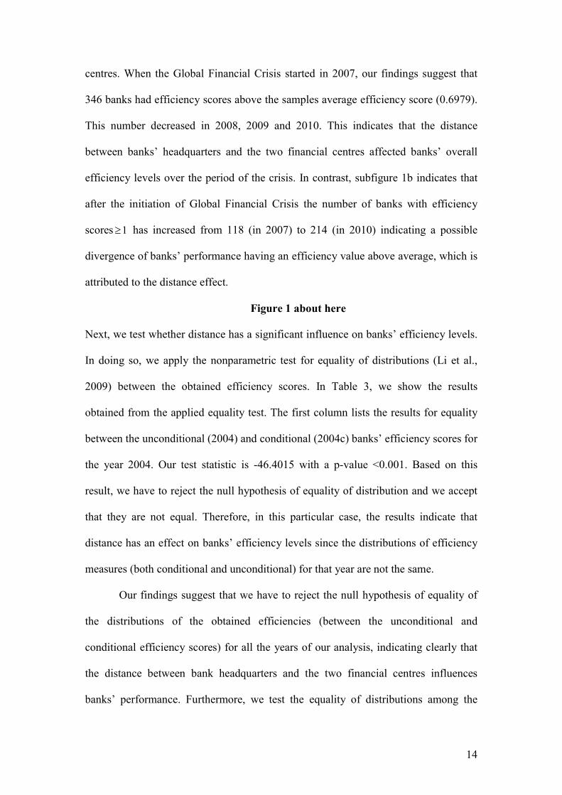
Our analysis continues in the same way, however, we examine the effect of
distance on banks’ performance by looking at the effect on banks with a distance to
the two financial centres that is lower than the average value (i.e for distances
between 5571 to 10540 km) and for banks with distances above the average distance
value (i.e. from 10,541 to 33,608 km). This allows us to magnify the effect of distance
on banks’ performance by breaking up our analysis into two subsamples.
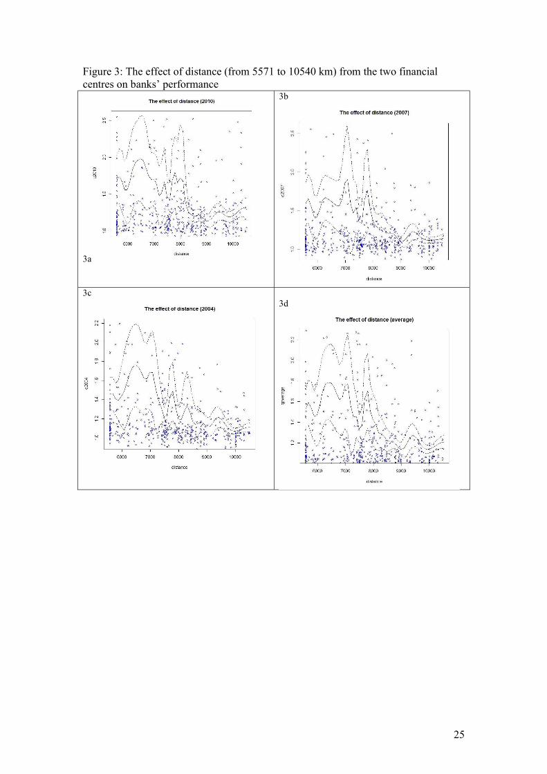
Figure 3 illustrates the effect of distance on banks’ performance for distances
from the two financial centres from 5,571 to 10,540 km. The effect is highly nonlinear
but with a decreasing trend, indicating a positive effect on bank performance. Since
our distance measure is the sum of the distance in kilometers from banks’
headquarters to the two financial centres it appears that being close to a financial
centre (given the fact that the minimum distance value is 5,571– the distance between
London and New York) has a positive effect. It appears that 10,000 km is the turning
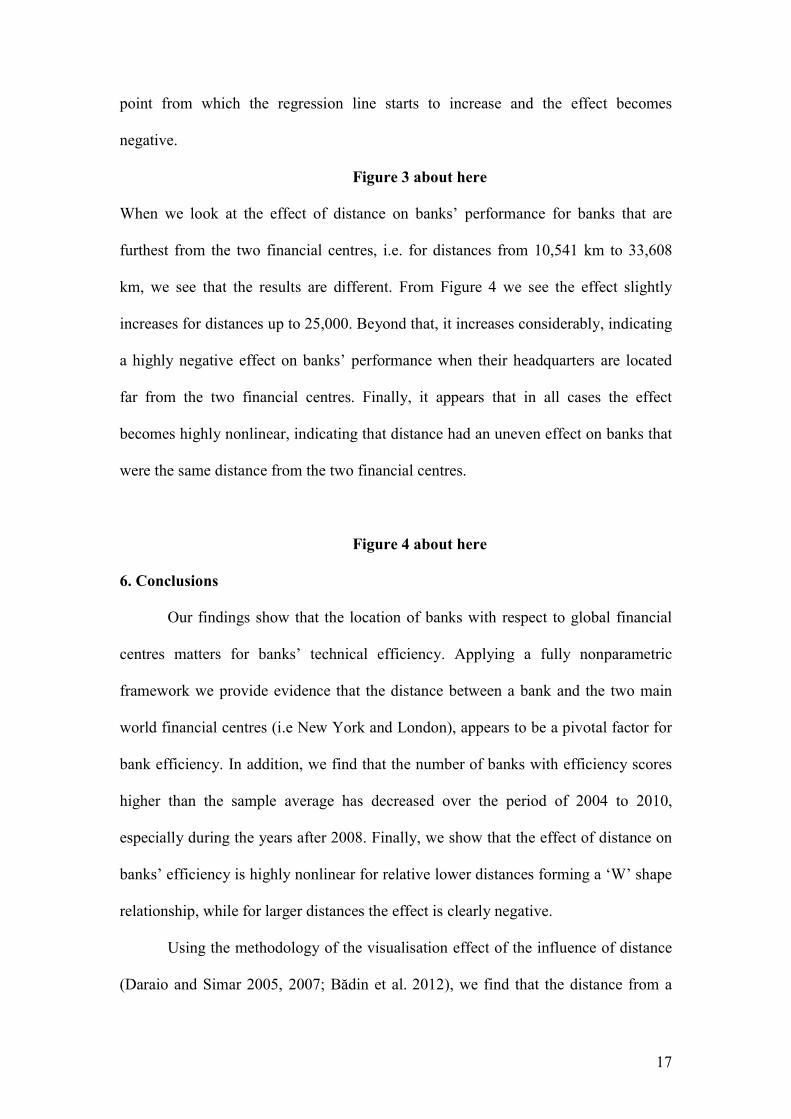
17
point from which the regression line starts to increase and the effect becomes
negative.
Figure 3 about here
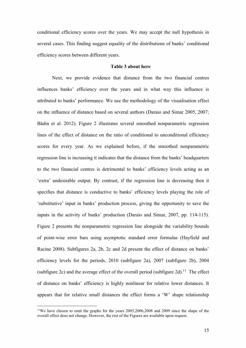
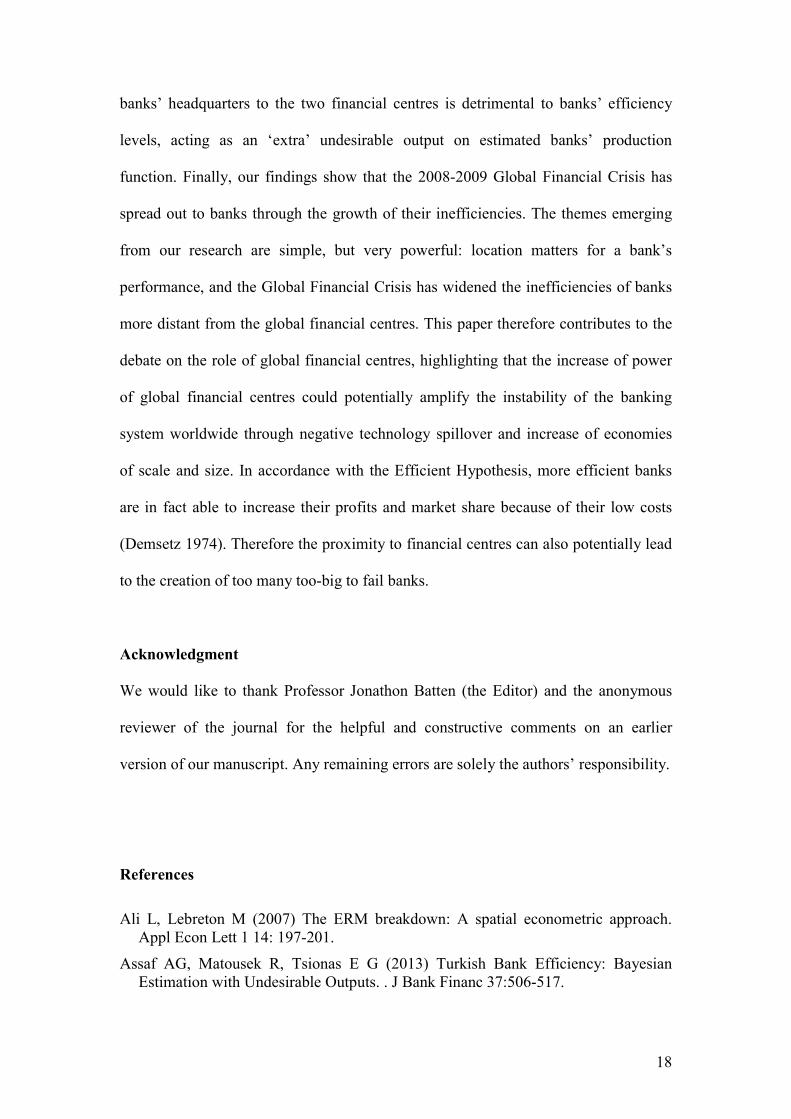
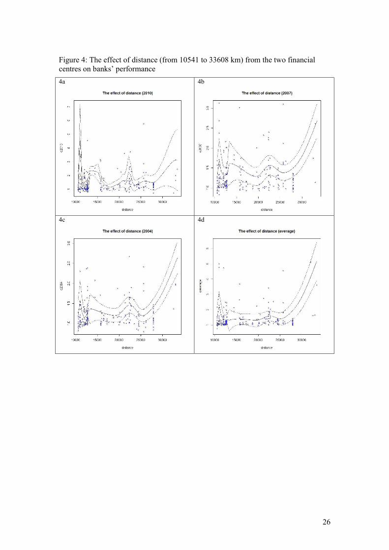
When we look at the effect of distance on banks’ performance for banks that are
furthest from the two financial centres, i.e. for distances from 10,541 km to 33,608
km, we see that the results are different. From Figure 4 we see the effect slightly
increases for distances up to 25,000. Beyond that, it increases considerably, indicating
a highly negative effect on banks’ performance when their headquarters are located
far from the two financial centres. Finally, it appears that in all cases the effect
becomes highly nonlinear, indicating that distance had an uneven effect on banks that
were the same distance from the two financial centres.
Figure 4 about here
6. Conclusions
Our findings show that the location of banks with respect to global financial
centres matters for banks’ technical efficiency. Applying a fully nonparametric
framework we provide evidence that the distance between a bank and the two main
world financial centres (i.e New York and London), appears to be a pivotal factor for
bank efficiency. In addition, we find that the number of banks with efficiency scores
higher than the sample average has decreased over the period of 2004 to 2010,
especially during the years after 2008. Finally, we show that the effect of distance on
banks’ efficiency is highly nonlinear for relative lower distances forming a ‘W’ shape
relationship, while for larger distances the effect is clearly negative.
Using the methodology of the visualisation effect of the influence of distance
(Daraio and Simar 2005, 2007; B<din et al. 2012), we find that the distance from a
18
banks’ headquarters to the two financial centres is detrimental to banks’ efficiency
levels, acting as an ‘extra’ undesirable output on estimated banks’ production
function. Finally, our findings show that the 2008-2009 Global Financial Crisis has
spread out to banks through the growth of their inefficiencies. The themes emerging
from our research are simple, but very powerful: location matters for a bank’s
performance, and the Global Financial Crisis has widened the inefficiencies of banks
more distant from the global financial centres. This paper therefore contributes to the
debate on the role of global financial centres, highlighting that the increase of power
of global financial centres could potentially amplify the instability of the banking
system worldwide through negative technology spillover and increase of economies
of scale and size. In accordance with the Efficient Hypothesis, more efficient banks
are in fact able to increase their profits and market share because of their low costs
(Demsetz 1974). Therefore the proximity to financial centres can also potentially lead
to the creation of too many too-big to fail banks.
Acknowledgment
We would like to thank Professor Jonathon Batten (the Editor) and the anonymous
reviewer of the journal for the helpful and constructive comments on an earlier
version of our manuscript. Any remaining errors are solely the authors’ responsibility.
References
Ali L, Lebreton M (2007) The ERM breakdown: A spatial econometric approach. Appl Econ Lett 1 14: 197-201.
Assaf AG, Matousek R, Tsionas E G (2013) Turkish Bank Efficiency: Bayesian Estimation with Undesirable Outputs. . J Bank Financ 37:506-517.
19
Black, D, Smith J (2004) How robust is the evidence on the effects of college quality? Evidence from matching. J. Econometrics 121: 99–124.
B<din L, Daraio C, Simar L (2010) Optimal bandwidth selection for conditional efficiency measures: A Data-driven approach. Eur J Oper Res 201: 633-640.
B<din L, Daraio C, Simar L (2012) How to measure the impact of environmental factors in a nonparametric production model? Eur J Oper Res 223: 818–833.
Baldwin R E, Okubo T (2006) Heterogeneous firms, agglomeration and economic geography: spatial selection and sorting. J Econ Geogr 6: 323–346.
Berger A N, DeYoung R (2001) The Effects of Geographic Expansion on Bank Efficiency. J Financ Serv Res 19: 163–84.
Berger A N, DeYoung R (2006) Technological Progress and the Geographic Expansion of the Banking Industry. ? J Money Credit Bank 38: 1483–513.
Berger A N, DeYoung R (1997) Problem loans and cost efficiency in commercial banks. J Bank Financ 21: 849–870.
Berger A N, Humphrey D B (1992) Competition, efficiency, and the future of the banking industry. In Proceedings, Federal Reserve Bank of Chicago, pp 629-655.
Berger A N, Humphrey D B (1997) Efficiency of financial institutions: International survey and directions for future research. Eur J Oper Res 98: 175-212.
Berger A N, Hanweck G A, Humphrey D B (1987) Competitive viability in banking: scale, scope, and product mix economies. J Monetary Econ 20: 501–520.
Boschma R A, Weterings A B R (2005) The effect of regional differences on the performance of software firms in the Netherlands. J Econ Geogr 5(5): 567-588.
Carey M, Nini G (2007) Is the Syndicated Loan Market Globally Integrated? J Financ 33: 389- 404.
Cassis Y (2010) Capitals of Capital: a History of International Financial Centres, 1780–2005, 2nd Ed., Cambridge: Cambridge University Press.
Cazals C, Florens J P, Simar L (2002) Nonparametric frontier estimation: a robust approach. J Econometrics 106: 1-25.
Cerqueiro G, Degryse H, Ongena S (2009) Distance, bank organizational structure, and lending decisions. In: Alessandrini P, Fratianni M, Zazzaro A (eds.). The changing geography of banking and finance, New York, Springer, pp 75-108.
Daraio C, Simar L (2005) Introducing environmental variables in nonparametric frontier models: A probabilistic approach. J Prod Anal 24: 93-121.
Daraio C, Simar L (2007). Advanced robust and nonparametric methods in efficiency analysis. Springer Science, New York.
Degryse H, Ongena S (2005) Distance, Lending Relationships, and Competition. J Financ 60: 231-266.
Dell’Ariccia G (2001) Asymmetric information and the structure of the banking industry. Eur Econ Rev 45(10): 1957–198.
Demsetz H (1974) Two Systems of Belief about Monopoly, in H. J. Goldschmid, H. M. Mann and J. F. Weston (eds), Industrial Concentration: the New Learning, Boston, MA, Little Brown, pp 164–184.
20
Deng S E, Elyasiani E (2008) Geographic diversification, bank holding, company value, and non-performing loans. ? J Money Credit Bank 40(6): 1217-1238.
Deprins D, Simar L, Tulkens H (1984). Measuring labor-efficiency in post offices. In: M., Marchand, P., Pestieau, H., Tulkens (Eds.), The Performance of public enterprises - Concepts and Measurement, pp 243-267. North-Holland, Amsterdam.
Devaney M, Weber W L (2002) Small-business lending and profit efficiency in commercial banking. J Financ Serv Res 22: 225–246.
Eichengreen B, Rose A K, Wyplosz C (1996). Contagious currency crises: First tests. Scandinavian J Econ 98: 463–484.
Engelen E, Grote M H (2009) Stock exchange virtualisation and the decline of second-tier financial centres—the cases of Amsterdam and Frankfurt. J Econ Geogr 9: 679-696.
Flannery M J, Kwan S H, Nimalendran M (2013) The 2007–2009 financial crisis and bank opaqueness. J Financ Intermed 22(11): 55-84.
French S, Leyshon A, Thrift N (2009) A very geographical crisis: the making and breaking of the 2007–2008 financial crisis. Cambridge J Reg, Econ and Soc 2: 1–17.
Frölich M (2008) Parametric and nonparametric regression in the presence of endogenous control variables. Int Stat Rev 76 (2): 214-227.
Fukuyama H, Matousek R (2011) Efficiency of Turkish banking: Two-stage network system. Variable returns to scale model. J. Int. Finance Markets Inst. Money 21:75-91.
Glick R, Rose A K (1999) Contagion and trade: Why are currency crises regional? J Int Money and Financ 18: 603–617.
Grote M H (2008) Foreign banks’ attraction to the financial centre Frankfurt—an inverted ‘U’-shaped relationship. J Econ Geogr 8: 239–258.
Hall P, Racine J S, Li Q (2004) Cross-validation and the estimation of conditional probability densities. J Am Stat Assoc 99: 1015–1026.
Hayfield T, Racine J S (2008) Nonparametric Econometrics: The np Package. J of Sta Software 27: 1-32.
Holod D, Lewis H F (2011) Resolving the deposit dilemma: A new DEA bank efficiency model. J Bank Financ 35: 2801-2810.
Hunter W C, Timme S G (1995) Core deposits and physical capital: a re-examination of bank scale economies and efficiency with quasi-fixed inputs. ? J Money Credit Bank 28: 165–185.
Krugman P (1991) Increasing returns and economic geography. J Polit Econ 99: 483-99.
Krugman P (1998). What’s new about the new economic geography? Oxford Rev Econ Pol 14(2): 7-17.
Lee R, Clark G, Pollard J, Leyshon A (2009) The remit of financial geography - before and after the crisis. J Econ Geogr 9: 723-747.
21
Li Q, Racine, J S (2004) Cross-validated local linear nonparametric regression. Statistica Sinica14: 485-512.
Li Q, Maasoumi E, Racine J S (2009) A Nonparametric Test for Equality of Distributions with Mixed Categorical and Continuous Data. J Econometrics 148: 186-200.
Martin R (2010) Local geographies of the financial crisis. J Econ Geogr 86: 1–32. Matousek, R., & Tzeremes, N. G. (2016). CEO compensation and bank efficiency: An
application of conditional nonparametric frontiers. Eur J Oper Res 251(1): 264-273.
McCauley R, McGuire P, Goetz P (2012) After the global financial crisis: from international to multinational banking? J Econ and Bus 64: 7-23.
Nadaraya E A (1965) On nonparametric estimates of density functions and regression curves. Theor Appl Probab 10: 186–190.
O’Brien R (1992) Global Financial Integration: The End of Geography. London: Pinter.
Pritzker M (2010) Informational easing: Improving credit conditions through the release of information. Federal Reserve Bank of New York Economic Policy Review 16: 77Ǧ88.
Salim R, Arjomandi A, Seufert JH (2016) Does corporate governance affect Australian banks’ performance? J. Int. Finance Markets Inst. Money 43: 113-125.
Sealey C W, Lindley J T (1977) Inputs, outputs, and a theory of production and cost at depository financial institutions. J Financ 32: 1251-1266.
Simar L (2003) Detecting outliers in frontiers models: a simple approach. J Prod Anal 20: 391–424.
Simar L, Wilson P W (2011) Two-stage DEA: caveat emptor. J Prod Anal 36: 205-218.
Simon H (1982) Models of Bounded Rationality, Vols. I and II. Cambridge, MA: MIT Press.
Stockhammer E (2008). Some stylized facts on the finance-dominated accumulation regime. Comp and Change, 12: 184–202.
Storper M, Venables A J (2004) Buzz: face-to-face contact and the urban economy. J Econ Geogr 4(4): 351-370.
Thrift N (1994) On the social and cultural determinants of international financial centres: the case of the city of London. In S. Corbridge, N. Thrift, R. Martin (eds) Money, Power and Space, pp 327–355. Oxford: Blackwell.
Tschoegl A E (2000) International Banking Centers, Geography, and Foreign Banks. Financ Mark Inst Instrum 9: 1-32.
Tsionas, E G, Assaf, A G, Matousek, R (2015). Dynamic technical and allocative efficiencies in European banking. J Bank Financ 52: 130-139.
Tzeremes N G (2014) The effect of human capital on countries' economic efficiency. Econ Lett 124(1): 127-131.

22
Tzeremes, N G (2015) Efficiency dynamics in Indian banking: A conditional directional distance approach. Eur J Oper Res 240(3): 807-818.
Wainwright T (2012) Number crunching: financialization and spatial strategies of risk organization. J Econ Geogr 12: 1267–1291.
Wanke P, Azad AK, Barros PC, Hassan KM (2016) Predicting efficiency in Islamic banks: An integrated multicriteria decision making (MCDM) approach. J. Int. Finance Markets Inst. Money, http://dx.doi.org/10.1016/j.intfin.2016.07.004.
Watson G S (1964) Smooth regression analysis. Sankhya 26: 359–372. Wójcik D (2013) The dark side of NY-LON: Financial centres and the Global
Financial Crisis. Urban Stud 50(13): 2736-2752.
23
Figure 1: Graphical representations of banks’ efficiency levels 1a
1b
Order-m efficiencies
380 386 378 368 365 364 355
70 61 62 65 72 81 99
050
100150
200250
300350
400450
500
2004 2005 2006 2007 2008 2009 2010
Years
Num
ber o
f Ban
ks
Number of Banks w ith Eficiency levels >=1
Number of Banks w ith Eficiency levels above mean value
Conditional to distance Order-m efficiencies
376295
364 346301 316 304
118178
104 118 207 175 214
0
100
200
300
400
500
600
2004 2005 2006 2007 2008 2009 2010
Years
Num
ber o
f Ban
ks
Number of Banks w ith Ef iciency levels >=1
Number of Banks w ith Ef iciency levels above mean value
24
Figure 2: The effect of distance (from 5571 to 33608 km) from the two financial centres on banks’ performance 2a
2b
2c
2d
25
Figure 3: The effect of distance (from 5571 to 10540 km) from the two financial centres on banks’ performance
3a
3b
3c
3d
26
Figure 4: The effect of distance (from 10541 to 33608 km) from the two financial centres on banks’ performance
4a
4b
4c
4d
27
Table 1: Descriptive statistics of the variables used
INPUTS OUTPUTS External variable
Number of Employees Fixed Assets Total Customer Deposits Gross Loans Total Securities Physical Distance
(Km)
Year 2010 Std 29233.485 1856636.813 127973919.4 112706506.2 111677075.9 6223.997
Mean 7578.043 466615.802 33477178.95 33217063.12 21723631.43 10540.37
Year 2009 Std 28064.156 1862321.129 113508685.5 103926125.3 105196938
Mean 7375.343 450473.704 30595337.46 31029157.87 20370005.4
Year 2008 Std 27839.935 1655172.127 100654362.5 95732721.71 142871126.7
Mean 7306.043 408976.963 27408197.46 29021273.33 23394613.72
Year 2007 Std 27190.329 1527275.619 96002366.81 95974172.89 116379944.8
Mean 7039.204 396474.544 26561473.22 28065688.95 20240870.09
Year 2006 Std 26411.946 1419823.092 81381608.16 77738921.03 88224886.22
Mean 6714.655 354447.503 22063330.1 22709673.43 15662524.88
Year 2005 Std 26509.204 1260648.092 68134589.57 62912067.16 82058223.37
Mean 6446.789 320725.872 18642898.62 18639783.03 13616554.78
Year 2004 Std 26627.474 1286278.315 62809269.67 59707226.77 89306912.44
Mean 6291.153 323555.828 17479987.73 17607719.49 14053127.15
28
Table 2: Descriptive statistics of the original and conditional order-m estimators
Original order-m efficiencies 2004 2005 2006 2007 2008 2009 2010
Mean 0.6496 0.6306 0.6378 0.6316 0.6502 0.6441 0.6578 Std 0.2994 0.2892 0.2914 0.2890 0.2932 0.2990 0.3143
Conditional order-m efficiencies Mean 0.7070 0.7863 0.6879 0.6979 0.8124 0.7652 0.8106 Std 0.3185 0.3854 0.3089 0.3160 0.3933 0.3686 0.4001
Table 3: Consistent density equality test for conditional order-m efficiency scores
Tn value 2005c 2006c 2007c 2008c 2009c 2010c 2004 vs 2004c -46.4015*** 2004c -196.74*** -130.586* -129.937* -155.1115*** -143.6456** -0.1395814*** 2005 vs 2005c -57.7482*** 2005c 174.8166 174.8273 88.9147 128.4527 320.0294 2006 vs 2006c -69.5176*** 2006c -0.81079 -61.76061* -33.3785 159.783 2007 vs 2007c -67.304*** 2007c -61.29818** -32.8031 160.2863 2008 vs 2008c -47.5852*** 2008c 35.23381 237.3271 2009 vs 2009c -54.9931*** 2009c 199.098 2010 vs 2010c -16.1412*** *** p-value < 0.001., ** p-value < 0.05; * p-value < 0.1

29
Recommended