Click to edit Master title style
1Copyright © NUMECA InternationalBenchmarkReport_2014-09-19_FM_Resistance-KCS
KCS Resistance Calculation
Author: Ludwig Kerner
Last update: 19-09-2014
Reviewed by : Jonathan Brunel
Date of Review : 19-09-2014
Click to edit Master title style
Copyright © NUMECA InternationalBenchmarkReport_2014-09-19_FM_Resistance-KCS2
Content
12
4
Test Case Description
Mesh Generation
Results3 Computations
0 Executive Summary
5 Conclusion

Click to edit Master title style
Copyright © NUMECA InternationalBenchmarkReport_2014-09-19_FM_Resistance-KCS3
This document presents the CFD calculation of the resistance of the KCS. A model scale hull was simulated in upright
conditions for different Froude numbers. The simulations (CAD import – meshing – computations – visualization) were
performed with FINETM/Marine, NUMECA’s Flow INtegrated Environment for marine applications, edited and
developed by NUMECA in partnership with ECN (Ecole Centrale de Nantes) and CNRS (Centre National de la Recherche
Scientifique).
The hull was downloaded in Parasolid format before importing it in HEXPRESS. The mesh was then generated with
HEXPRESSTM , NUMECA’s full hexahedral unstructured grid generator integrated in FINETM/Marine.
Results were processed and analyzed with CFViewTM, NUMECA’s Flow Visualization System integrated in
FINETM/Marine.
Executive Summary

Click to edit Master title style
Copyright © NUMECA InternationalBenchmarkReport_2014-09-19_FM_Resistance-KCS4
FINETM/Marine
<Grid generator:
HEXPRESSTM
Free surface flow solver:
ISIS-CFD
Post-processor:
CFViewTM
GUI
Flow INtegrated Environment for Marine Applications

Click to edit Master title style
Copyright © NUMECA InternationalBenchmarkReport_2014-09-19_FM_Resistance-KCS5
Workflow
Meshing
HEXPRESSTM
Computation Set-up
FINETM GUI
Computation
ISIS-CFD
Post-processing
CFViewTM

Click to edit Master title style
Copyright © NUMECA InternationalBenchmarkReport_2014-09-19_FM_Resistance-KCS6
Test Cases Description

Click to edit Master title style
Copyright © NUMECA InternationalBenchmarkReport_2014-09-19_FM_Resistance-KCS7
The geometry studied is a model scale of the KCS. The table below shows the main characteristics of the vessel at full
scale.
KCS Description
3D view of model
Main particulars Full scale
Length between perpendiculars LPP (m) 230.0
Length of waterline LWL (m) 232.5
Maximum beam of waterline BWL (m) 32.2
Depth D (m) 19.0
Draft T (m) 10.8
Displacement &Delta (m3 ) 52030
Wetted area w/o rudder SW (m2 ) 9424
Wetted surface area of rudder SR (m2 ) 115.0
Block coefficient (CB)&Delta /(LPPBWL T) 0.6505
Midship section coefficient (CM) 0.9849
LCB (%LPP), fwd+ -1.48
Vertical Center of Gravity (from keel) KG (m) 7.28
Metacentric height GM (m) 0.60
Moment of Inertia Kxx/B 0.40
Moment of Inertia Kyy/LPP, Kzz/LPP 0.25
Propeller center, long. location (from FP) x/LPP 0.9825
Propeller center, vert. location (belowWL) -z/LPP 0.02913

Click to edit Master title style
Copyright © NUMECA InternationalBenchmarkReport_2014-09-19_FM_Resistance-KCS8
The computation referred to the towing tank tests performed by MOERI on the KCS. The length between
perpendiculars is 7.2786 m (scale factor = 31.6) and the body draft is 0.3418 m. The water density considered is 999.1
kg/ m³. The position of the center of gravity along X axis has been estimated using the tool “domhydro” resulting in a
location (X=-11.7, Y=0, Z=-0.115) in the global reference frame. The model contains the hull and the rudder of the KCS.
The first case referred to the case 2_1 of the 2010 Gothenburg workshop. The vessel is moving with a
speed of 2.196 m/s (corresponding to a Froude number of 0.26) . In these cases, the trim and the sinkage are blocked.
The geometry contains only the hull. The output of the first calculation will be :
- Wave elevation along longitudinal section
- Wave elevation along the hull
- Wave elevation contours
- Axial velocity and cross flow near the engine shaft
The second calculation referred to the cases 2_2a of the Gothenburg workshop. it concerns the
resistance calculation of the KCS while it is moving with a speed of 2.196 m/s. The trim and the sinkage are still
blocked. The only difference with the previous case is the rudder which is present for the second case and not for the
first. The output of this calculation will be :
- Drag comparison with experimental data
- Visualization of the free surface
- Wetted area
- Hydrodynamic pressure on the hull
Test Case Description

Click to edit Master title style
Copyright © NUMECA InternationalBenchmarkReport_2014-09-19_FM_Resistance-KCS9
The third case referred to the case 2_2b of the Gothenburg workshop. It concerns the resistance
calculation of the KCS at different speeds from 0.92 m/s to 2.38 m/s (corresponding to a variation of the Froude
number from 0.1083 to 0.2816) . In this case, the trim and the sinkage are solved. In terms of output, the following
will be presented:
- Drag, Trim and Sinkage comparison with experimental data
- Visualization of the free surface
- Wetted area
- Hydrodynamic pressure on the hull
As the conditions of all cases are symmetric only half of the geometry is simulated.
Test Case Description

Click to edit Master title style
Copyright © NUMECA InternationalBenchmarkReport_2014-09-19_FM_Resistance-KCS10
Mesh Generation

Click to edit Master title style
Copyright © NUMECA InternationalBenchmarkReport_2014-09-19_FM_Resistance-KCS11
The Parasolid file is loaded into HEXPRESSTM. A computational domain is constructed by defining a box around the
model.
Commonly, we take the following dimensions
away from the model in terms of Lpp :
Front 1 x Lpp
Back 3 x Lpp
Top 0.5 x Lpp
Bottom 1.5 x Lpp
Each side 1.5 x Lpp
Mesh GenerationDomain Definition
Case 1
Case 2

Click to edit Master title style
Copyright © NUMECA InternationalBenchmarkReport_2014-09-19_FM_Resistance-KCS12
Mesh generation in HEXPRESSTM is done using a five-steps wizard:
Mesh GenerationMesh Wizard
Step 1:Initial meshan isotropic, Cartesian mesh is generated.
Step 2: Adapt to geometrythe mesh is refined in regions of interest by splitting the initial
volumes.
Step 3: Snap to geometryThe volumic, refined mesh is snapped onto the model.
Step 4:After snapping, the mesh can contain some
negative, concave, or twisted cells. This step will fix those cells and increase the quality of
the mesh.
Step 5:To capture viscous
effects, this step inserts viscous layers in the Eulerian mesh.

Click to edit Master title style
Copyright © NUMECA InternationalBenchmarkReport_2014-09-19_FM_Resistance-KCS13
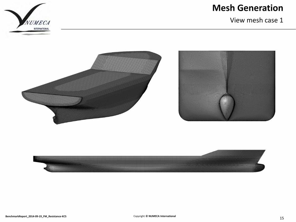
Two meshes are needed. A first one without the rudder for the case 1 and a second mesh with the rudder for the case
2 and 3. The meshes are quite fine and have the following properties:
The initial mesh size is 2500 cells
An internal surface is used to spatially discretize the region around the initial free surface. This surface is
located at z = 0,3417m and covers the whole domain. Mesh refinement normal to the free surface is set at
0.07m (Lpp / 1000). A local diffusion of 4 is used to ensure the free surface capturing during the computation.
For the viscous layers, the initial spacing is set at 1.476e-3m (ensuring a y+ of about 30). The stretching ratio is
set at 1.2. An inflation technique is used to find the optimum number of layers, ensuring a smooth transition
from viscous inner to outer Eulerian mesh. The viscous layers are inserted using the maximum velocity as
reference for both cases, as the same meshes will be used to run the complete set of conditions in the future.
Mesh GenerationSettings

Click to edit Master title style
Copyright © NUMECA InternationalBenchmarkReport_2014-09-19_FM_Resistance-KCS14
In the table below, the mesh characteristics for the vessel with rudder are listed. The repartition of cells for differentcriteria are also shown.
Mesh GenerationOverview
Mesh characteristic
Number of cell in Eulerian mesh [-]
1,724,459
Number of cells with viscous layers [-]
2,173,232
Minimal orthogonality [deg] 13.71
Maximal aspect ratio [-] 136.85
Maximal expansion ratio [-] 7.62
Click to edit Master title style
Copyright © NUMECA InternationalBenchmarkReport_2014-09-19_FM_Resistance-KCS15
Mesh GenerationView mesh case 1

Click to edit Master title style
Copyright © NUMECA InternationalBenchmarkReport_2014-09-19_FM_Resistance-KCS16
Mesh GenerationView mesh case 2

Click to edit Master title style
Copyright © NUMECA InternationalBenchmarkReport_2014-09-19_FM_Resistance-KCS17
Computations

Click to edit Master title style
Copyright © NUMECA InternationalBenchmarkReport_2014-09-19_FM_Resistance-KCS18
The FINE/Marine solver main features are:
3D, face –based approach, pressure equation formulation (SIMPLE)
Free surface capturing strategy with high-resolution interface schemes
Spatial discretization: upwind, hybrid, centered, blended, and Gamma (GDS)
Time discretization: steady, 1st and 2nd order backward schemes
Adaptive grid refinement
External forces (towing and wind effects), mooring or tugging lines
6 degrees of freedom with strong coupling, mesh deformation algorithm
Modeling of propeller using actuator disk theory
Sliding grids for multi-domain simulations
Euler and Navier-Stokes flows, Laminar and turbulent, steady and unsteady flow problems
Turbulence modeling:
• Spalart-Allmaras one-equation model
• Launder-Sharma k-ε model
• SST k-ω model
• BSL k-ω model
• Wilcox k-ω model
• EASM (Explicit Algebraic Stress Model)
All models can be used with low Reynolds formulation, wall functions, or rotation correction, except
the Spalart-Allmaras model (only available in low-Reynolds formulation)
On top of FINETM/Marine native formats, the solver also reads ICEM CFD and Gridgen meshes. Export
to Tecplot, EnSight, FieldView and CGNS formats
Computations
Introduction

Click to edit Master title style
Copyright © NUMECA InternationalBenchmarkReport_2014-09-19_FM_Resistance-KCS19
For Case 1, a symmetric computation, the following boundary conditions are used:
Computations
Boundary Conditions
Outlet: far field condition
Side: far field condition
Bottom: pressured imposed
Hull & Rudder: wall functionDeck: slip condition
Inlet: far field condition
Top: pressured imposed
Mirror plane: Mirror condition

Click to edit Master title style
Copyright © NUMECA InternationalBenchmarkReport_2014-09-19_FM_Resistance-KCS20
The computations settings common to the two cases are:
Common settings:
Time scheme: backward order 1
K-omega SST turbulence model with wall functions
Multi-fluid computation:
WATER: - Dynamic viscosity: 1.0122 (N s/m2) x 10-3
- Density: 999.1 kg/m3
AIR: - Dynamic viscosity: 1.85 (N s/m2) x 10-5
- Density: 1.2 kg/m3
Computations
Set-up
Ship characteristics
Lref (m) 7.2786
Y+ 30
Mass (Kg) 1652
Coordinates of the CoG (m) (3.53, 0.0,0.23)
Initial free surface location (m) 0.3418

Click to edit Master title style
Copyright © NUMECA InternationalBenchmarkReport_2014-09-19_FM_Resistance-KCS21
For the case 1 and 2, trim and sinkage are blocked. Only one speed is studied and the settings is summarized below :
For the case 3, trim and sinkage are solved. 6 speeds are studied to plot the resistance curve of the KCS. The tablebelow summarizes the settings :
Computations
Set-up
Case 1 and case 2
Vref [m/s] 2.196
Froude 0.2599
Time step [s] 0.018
Acceleration time [s] 3.51
Case 3
Vref [m/s] 0.915 1.281 1.647 1.921 2.196 2.379
Froude 0.1083 0.1516 0.1949 0.2274 0.2599 0.2816
Time step [s]
0.042 0.030 0.023 0.020 0.018 0.016
Acceleration time [s]
8.43 6.02 4.69 4.02 3.51 3.24

Click to edit Master title style
Copyright © NUMECA InternationalBenchmarkReport_2014-09-19_FM_Resistance-KCS22
Results case 1

Click to edit Master title style
Copyright © NUMECA InternationalBenchmarkReport_2014-09-19_FM_Resistance-KCS23
Results: Case I
Wave elevation
The wave elevation on the hull has been measured along a section situated at y/Lpp = 0.0741. The
experimental values (EFD) and computational results (CFD) results are superimposed to allow comparison.
-0,008
-0,006
-0,004
-0,002
0
0,002
0,004
0,006
-0,50 0,00 0,50 1,00 1,50 2,00
wav
e e
leva
tio
n /
Lp
p
x/Lpp
Wave elevation at y/Lpp = 0.0741
CFD
EFD
Y/Lpp = 0.0741

Click to edit Master title style
Copyright © NUMECA InternationalBenchmarkReport_2014-09-19_FM_Resistance-KCS24
-0,005
-0,004
-0,003
-0,002
-0,001
0
0,001
0,002
0,003
0,004
0,005
-0,5 0 0,5 1 1,5 2
wav
e e
leva
tio
n /
Lp
p
x/Lpp
wave elevation at y/Lpp = 0.1509
CFD
EFD
Results: Case I
Wave elevation
The wave elevation on the hull has been measured along a section situated at y/Lpp = 0.1509. The
experimental values and CFD results are superimposed to allow comparison.
Y/Lpp = 0.1509

Click to edit Master title style
Copyright © NUMECA InternationalBenchmarkReport_2014-09-19_FM_Resistance-KCS25
Results: Case I
Wave elevation
The wave elevation on the hull has been measured along a section situated at y/Lpp = 0.4224. The
experimental values and CFD results are superimposed to allow comparison.
Y/Lpp = 0.4224
-0,004
-0,003
-0,002
-0,001
0
0,001
0,002
0,003
0,004
-0,500 0,000 0,500 1,000 1,500 2,000
wav
e e
leva
tio
n /
Lp
p
x/Lpp
Wave elevation at y/Lpp = 0.4224
CFD
EFD

Click to edit Master title style
Copyright © NUMECA InternationalBenchmarkReport_2014-09-19_FM_Resistance-KCS26
Results: Case I
Wave elevation
The wave elevation on the hull has been measured and plotted. The experimental values are superimposed
to this result to allow comparison.
-0,008-0,006-0,004-0,002
00,0020,0040,0060,008
0,010,0120,014
0,00 0,10 0,20 0,30 0,40 0,50 0,60 0,70 0,80 0,90 1,00
wav
e e
leva
tio
n /
Lp
p
x/Lpp
Wave elevation on the hull
CFD
EFD

Click to edit Master title style
Copyright © NUMECA InternationalBenchmarkReport_2014-09-19_FM_Resistance-KCS27
Results: Case II
Wave elevation
The views below shows the wave elevation divided by Lpp. Above is the FINE™/Marine computation and
below is the experimental result provided to the participants of the Gothenburg workshop in 2010.
FINE™/Marine result
Experimentalresult

Click to edit Master title style
Copyright © NUMECA InternationalBenchmarkReport_2014-09-19_FM_Resistance-KCS28
Results: Case II
Speed field
The views below show the relative axial velocity divided by Lpp on the right panels and cross flow vectors and
streamlines on the left panels. The cutting plane is situated at x/Lpp = 0.9825 from the AP. The view above
has been realized in CFView and the view below is the experimental result.
FINE™/Marine result
Experimentalresult

Click to edit Master title style
Copyright © NUMECA InternationalBenchmarkReport_2014-09-19_FM_Resistance-KCS29
Effect of the turbulence model

Click to edit Master title style
Copyright © NUMECA InternationalBenchmarkReport_2014-09-19_FM_Resistance-KCS30
Effect of turbulence model
Comparison of wave elevation
In this section, we test the effect of the turbulence model on the result of the case 1. To this aim, we relaunch
the calculation with the EASM model instead of the kω-SST. The same post processing as for the previous
calculation is done and results are compared. The charts below compare wave elevation along sections
obtained with different turbulence model and the experimental data. We can see that both models give
exactly the same results.

Click to edit Master title style
Copyright © NUMECA InternationalBenchmarkReport_2014-09-19_FM_Resistance-KCS31
Effect of turbulence model
Comparison of wave elevation
The charts below compare wave elevation along sections obtained with different turbulence model and the
experimental data. We can see that both models give exactly the same results.

Click to edit Master title style
Copyright © NUMECA InternationalBenchmarkReport_2014-09-19_FM_Resistance-KCS32
Effect of turbulence model
Comparison of wave elevation
The views below shows the wave elevation divided by Lpp. Above is the result obtained with the turbulence
model K-ω-SST and below with the EASM model. We can see that the isolines match perfectly. The free
surfaces are quite the same.
FINE™/Marine K-ω-SST
FINE™/Marine EASM
Click to edit Master title style
Copyright © NUMECA InternationalBenchmarkReport_2014-09-19_FM_Resistance-KCS33
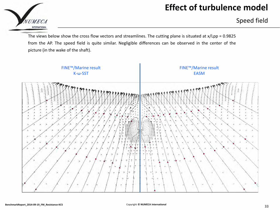
Effect of turbulence model
Speed field
The views below show the cross flow vectors and streamlines. The cutting plane is situated at x/Lpp = 0.9825
from the AP. The speed field is quite similar. Negligible differences can be observed in the center of the
picture (in the wake of the shaft).
FINE™/Marine resultK-ω-SST
FINE™/Marine resultEASM

Click to edit Master title style
Copyright © NUMECA InternationalBenchmarkReport_2014-09-19_FM_Resistance-KCS34
Effect of turbulence model
Speed field
The views below show the relative axial velocity divided by Lpp. The cutting plane is still situated at x/Lpp =
0.9825 from the AP. The shapes of the isolines are similar but we can observe little differences.
FINE™/Marine resultK-ω-SST
FINE™/Marine resultEASM
Click to edit Master title style
Copyright © NUMECA InternationalBenchmarkReport_2014-09-19_FM_Resistance-KCS35
Results case 2

Click to edit Master title style
Copyright © NUMECA InternationalBenchmarkReport_2014-09-19_FM_Resistance-KCS36
Results: Case II
Convergence
Overview of the convergence history
Computation time to convergence :-Convergence 1 %: 9 h on 16 partitions-Convergence 2 %: 8 h on 16 partitions
Converged simulation (less than 1% oscillation)
Converged simulation (less than 2% oscillation)
Click to edit Master title style
Copyright © NUMECA InternationalBenchmarkReport_2014-09-19_FM_Resistance-KCS37
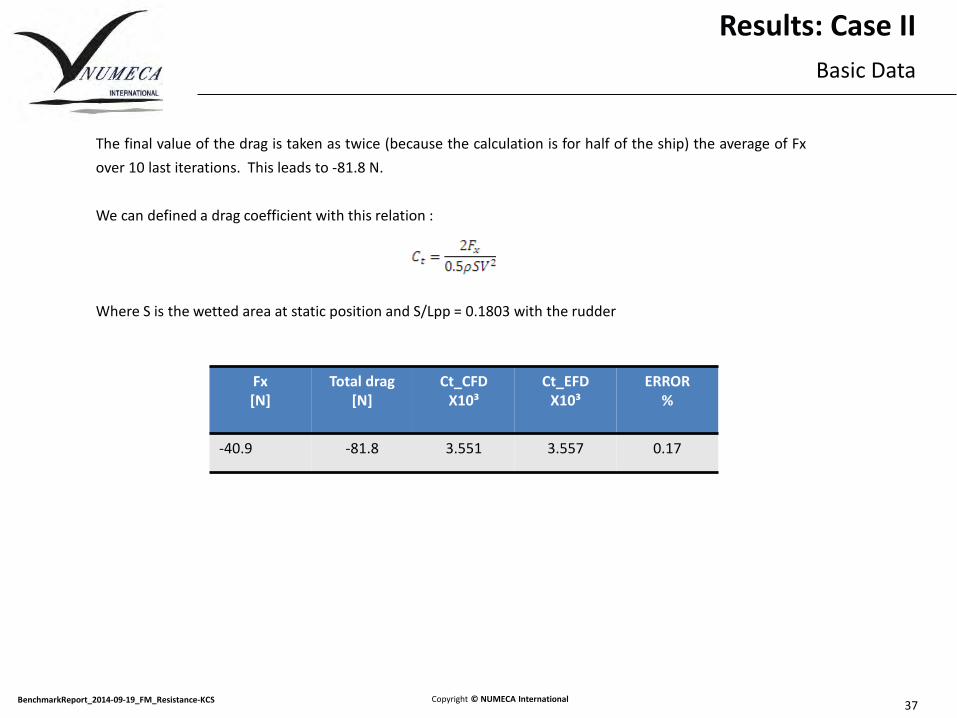
Results: Case II
Basic Data
The final value of the drag is taken as twice (because the calculation is for half of the ship) the average of Fx
over 10 last iterations. This leads to -81.8 N.
We can defined a drag coefficient with this relation :
Where S is the wetted area at static position and S/Lpp = 0.1803 with the rudder
Fx[N]
Total drag[N]
Ct_CFDX10³
Ct_EFDX10³
ERROR %
-40.9 -81.8 3.551 3.557 0.17

Click to edit Master title style
Copyright © NUMECA InternationalBenchmarkReport_2014-09-19_FM_Resistance-KCS38
Results: Case II
Wave Elevation

Click to edit Master title style
Copyright © NUMECA InternationalBenchmarkReport_2014-09-19_FM_Resistance-KCS39
Results: Case II
Wetted Surface
See figure below for a display (blue is air, red water).
In CFView, the wetted surface has been computed and
is equal to 4.91 m².

Click to edit Master title style
Copyright © NUMECA InternationalBenchmarkReport_2014-09-19_FM_Resistance-KCS40
Results: Case II
Hydrodynamic Pressure
See figure below for a display.
Click to edit Master title style
Copyright © NUMECA InternationalBenchmarkReport_2014-09-19_FM_Resistance-KCS41
Results case 3

Click to edit Master title style
Copyright © NUMECA InternationalBenchmarkReport_2014-09-19_FM_Resistance-KCS42
Results: Case III
Basic Data
See below for the basic data extracted from the computations .
ComparisonFr CT_efd
X10³
CT_cfd
X10³
error %
error
0.1083 3.80 3.73 -1.85 -0.07
0.1516 3.64 3.60 -1.24 -0.05
0.1949 3.48 3.46 -0.55 -0.02
0.2274 3.47 3.49 0.61 0.02
0.2599 3.71 3.70 -0.40 -0.01
0.2816 4.50 4.52 0.39 0.02

Click to edit Master title style
Copyright © NUMECA InternationalBenchmarkReport_2014-09-19_FM_Resistance-KCS43
Results: Case II
Wave Elevation
Fr = 0.1083 Fr = 0.1516 Fr = 0.1949
Fr = 0.2274 Fr = 0.2599 Fr = 0.2816

Click to edit Master title style
Copyright © NUMECA InternationalBenchmarkReport_2014-09-19_FM_Resistance-KCS44
Results: Case III
Wetted Surface
The table below summarize the wetted surface of the hull obtained for different speeds :
Wetted Surface
Froude 0.1083 0.1516 0.1949 0.2274 0.2599 0.2816
WettedSurface (m²)
9.78 9.84 9.92 9.98 10.06 10.12

Click to edit Master title style
Copyright © NUMECA InternationalBenchmarkReport_2014-09-19_FM_Resistance-KCS45
Results: Case III
Wetted Surface
Fr = 0.1083
Fr = 0.1516
Fr = 0.1949
Fr = 0.2274
Fr = 0.2599
Fr = 0.2816

Click to edit Master title style
Copyright © NUMECA InternationalBenchmarkReport_2014-09-19_FM_Resistance-KCS46
Results: Case III
Wetted Surface
Fr = 0.1083
Fr = 0.1516
Fr = 0.1949
Fr = 0.2274
Fr = 0.2599
Fr = 0.2816

Click to edit Master title style
Copyright © NUMECA InternationalBenchmarkReport_2014-09-19_FM_Resistance-KCS47
Results: Case III
Hydrodynamic Pressure
Fr = 0.1083
Fr = 0.1516
Fr = 0.1949
Fr = 0.2274
Fr = 0.2599
Fr = 0.2816

Click to edit Master title style
Copyright © NUMECA InternationalBenchmarkReport_2014-09-19_FM_Resistance-KCS48
Results: Case III
Hydrodynamic Pressure
Fr = 0.1083
Fr = 0.1516
Fr = 0.1949
Fr = 0.2274
Fr = 0.2599
Fr = 0.2816

Click to edit Master title style
Copyright © NUMECA InternationalBenchmarkReport_2014-09-19_FM_Resistance-KCS49
Reduction of the
computational time

Click to edit Master title style
Copyright © NUMECA InternationalBenchmarkReport_2014-09-19_FM_Resistance-KCS50
In this part of the presentation, we want to know how fast FINE™/Marine can be to finish the resistance calculation.
To this aim, we have selected the speed of 1.65 m/s and calculations have been launched with different settings. The
numerical parameter that we want to study is the number of non-linear iterations. We also want to know if the sub-
cycling acceleration method is interesting. The combination of these two parameters leads to 8 calculations
summarized below :
- number of non-linear iterations of 2 without sub-cycling
- number of non-linear iterations of 2 with sub-cycling
- number of non-linear iterations of 3 without sub-cycling
- number of non-linear iterations of 3 with sub-cycling
- number of non-linear iterations of 4 without sub-cycling
- number of non-linear iterations of 4 with sub-cycling
- number of non-linear iterations of 5 without sub-cycling
- number of non-linear iterations of 5 with sub-cycling
Reduction of computational costList of calculations
Click to edit Master title style
Copyright © NUMECA InternationalBenchmarkReport_2014-09-19_FM_Resistance-KCS51
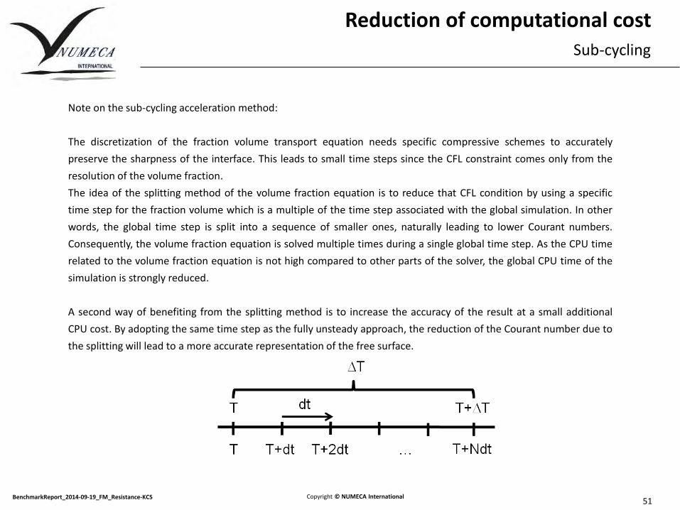
Reduction of computational cost
Note on the sub-cycling acceleration method:
The discretization of the fraction volume transport equation needs specific compressive schemes to accurately
preserve the sharpness of the interface. This leads to small time steps since the CFL constraint comes only from the
resolution of the volume fraction.
The idea of the splitting method of the volume fraction equation is to reduce that CFL condition by using a specific
time step for the fraction volume which is a multiple of the time step associated with the global simulation. In other
words, the global time step is split into a sequence of smaller ones, naturally leading to lower Courant numbers.
Consequently, the volume fraction equation is solved multiple times during a single global time step. As the CPU time
related to the volume fraction equation is not high compared to other parts of the solver, the global CPU time of the
simulation is strongly reduced.
A second way of benefiting from the splitting method is to increase the accuracy of the result at a small additional
CPU cost. By adopting the same time step as the fully unsteady approach, the reduction of the Courant number due to
the splitting will lead to a more accurate representation of the free surface.
Sub-cycling

Click to edit Master title style
Copyright © NUMECA InternationalBenchmarkReport_2014-09-19_FM_Resistance-KCS52
Reduction of computational cost
In order to quantify the computational cost, we define a quantity that we want to reduce :
Computational cost = time to reach the convergence * number of processor on which the calculation has run
Computational cost
Nb of non-linear
iterations
subcycling Time per time step [s] nb of timstep for convergence 1%
nb of timstep for convergence 2%
nb of proc cpu cost [cpu.h]Convergence 1%
cpu cost [cpu.h]Convergence 2%
2 no 8.52 4661 3605 16 176.5 136.5
2 yes 13.10 860 775 16 50.1 45.1
3 no 12.92 3079 1935 16 176.9 111.1
3 yes 19.24 539 475 16 46.1 40.6
4 no 17.14 2197 1537 16 167.4 117.1
4 yes 26.00 420 307 16 48.5 35.5
5 no 20.56 1935 1405 16 176.8 128.4
5 yes 21.80 352 292 16 34.1 28.3

Click to edit Master title style
Copyright © NUMECA InternationalBenchmarkReport_2014-09-19_FM_Resistance-KCS53
Reduction of computational cost
Finally, the fastest calculation is the one combining 5 non-linear iteration and the sub-cycling. It has a computational
cost of about 30 cpu.h, which means approximately that the calculation can converge in 1h on 30 processors.
The computational cost is plotted on the chart below. We can see that the sub-cycling option allows to reduce the
computational cost by 4, passing from 176.8 h.cpu to 34.1 h.cpu
The number of non-linear iteration has only a little impact on the computational cost when it varies between 2 and 5.
Computational cost
Click to edit Master title style
Copyright © NUMECA InternationalBenchmarkReport_2014-09-19_FM_Resistance-KCS54
Conclusion

Click to edit Master title style
Copyright © NUMECA InternationalBenchmarkReport_2014-09-19_FM_Resistance-KCS55
This case covers a wide part of the FINETM/Marine features and demonstrates the ability of the product to handle this
kind of project in a short time frame.
Conclusion
<Grid generator:
HEXPRESSTM
Free surface flow solver:
ISIS-CFD
Post-processor:
CFViewTM
GUI

Click to edit Master title style
Copyright © NUMECA InternationalBenchmarkReport_2014-09-19_FM_Resistance-KCS56
It is shown in this work that FINE/Marine is:
• Accurate
• Dedicated to Marine applications
• Very fast in meshing: 2.3 million s of cells in 5 minutes
• Very fast computing time: 1 hour of CPU time using 32 cores PC on 2.3 million of cells
• Dedicated post-processing
• Seamless automated design process can be integrated into existing customers’working process
Conclusion

Click to edit Master title style
57Copyright © NUMECA InternationalBenchmarkReport_2014-09-19_FM_Resistance-KCS
Open Discussion
KCS Resistance Calculation
Recommended