1
TUNA-DOLPHIN-BIRD FEEDING ASSEMBLAGES IN THE GALAPAGOS
ISLANDS AND THEIR RESPONSE TO THE PHYSICAL
CHARACTERISTICS OF THE UPPER WATER COLUMN
A Thesis
by
MICHELLE LYNN JOHNSTON
Submitted to the Office of Graduate Studies of
Texas A&M University
in partial fulfillment of the requirements for the degree of
MASTER OF SCIENCE
August 2011
Major Subject: Oceanography

2
Tuna-Dolphin-Bird Feeding Assemblages in the Galapagos Islands and Their Response
to the Physical Characteristics of the Upper Water Column
Copyright 2011 Michelle Lynn Johnston

3
TUNA-DOLPHIN-BIRD FEEDING ASSEMBLAGES IN THE GALAPAGOS
ISLANDS AND THEIR RESPONSE TO THE PHYSICAL
CHARACTERISTICS OF THE UPPER WATER COLUMN
A Thesis
by
MICHELLE LYNN JOHNSTON
Submitted to the Office of Graduate Studies of
Texas A&M University
in partial fulfillment of the requirements for the degree of
MASTER OF SCIENCE
Approved by:
Chair of Committee, Douglas Biggs
Committee Members, John Wormuth
William Neill
Head of Department, Piers Chapman
August 2011
Major Subject: Oceanography

iii
ABSTRACT
Tuna-Dolphin-Bird Feeding Assemblages in the Galapagos Islands and Their Response
to the Physical Characteristics of the Upper Water Column. (August 2011)
Michelle Lynn Johnston, B.S., Westminster College
Chair of Advisory Committee: Dr. Douglas Biggs
Tuna-dolphin-bird feeding assemblages are unique to the Eastern Tropical Pacific
Ocean (ETP). These multiple species groups are believed to forage together in response
to the physical properties of the near surface ocean as these constrain the distribution of
prey. In the Galapagos Marine Reserve (GMR), intra-annual and interannual changes
affect the properties of the water column, inducing mesoscale and fine scale temporal
variability. Four three-week oceanographic surveys took place, in September 2008,
April 2009, October 2009, and September 2010, between the coast of Ecuador and the
Galapagos Islands and one small boat survey took place in June 2010 within the GMR.
Marine mammal surveys were conducted during daylight hours and Conductivity,
Temperature, Depth (CTD) sensor casts were taken throughout the survey. Data were
analyzed to determine the types of water masses present and the strength and depth of
the thermocline layer. These data were compared with the sightings of marine
mammals, bird feeding groups, and tuna-dolphin-bird assemblages. Additionally, these
data were used to predict where tuna would be likely to associate with dolphin groups.
Results show Equatorial Surface Water was the dominant water mass throughout

iv
iv
the archipelago, regardless of season or ENSO index. High salinity, cold water west of
Isla Isabela indicated topographic upwelling of the Equatorial Undercurrent. Tropical
Surface Waters from the Panama Current were detected north of the Equatorial Front to
the east of the islands. Obvious changes in the water column properties were observed
between El Niño and La Niña events in the GMR.
Most mixed groups were sighted west and south of Isla Isabela during the four
oceanographic surveys, as well as north and west of Isla San Cristobal in June 2010.
Most sightings were in cool, high salinity waters, and high chlorophyll concentrations.
There were a greater number of sightings during the April 2009 survey (ENSO-neutral
conditions) than during any of the three fall surveys. Additionally, tuna-dolphin-bird
groups were more likely to be seen near Isla Isabela, with the majority of them sighted
during the April 2009 survey and a few sighted in each of the September 2008 and
October 2009 surveys. No tuna-dolphin-bird groups were sighted during the September
2010 surveys. Results show that the presence and location of these multi-species groups
may be controlled by the inter-annual cycles, the intra-annual cycles, or a combination of
both types of changes seen within the Galapagos.

v
v
I would like to dedicate this thesis to my family and friends for all of their support in my
studies.

vi
vi
ACKNOWLEDGEMENTS
This project was supported by a variety of people and organizations, without
which it would have been impossible to complete. Funding was provided by the
Department of Oceanography, the Office of Graduate Studies, and Dr. Biggs. I would
like to acknowledge Dr. Biggs for his guidance in the development of this project and
manuscript. My committee members, Dr. Neill and Dr. Wormuth, offered helpful
comments and help in writing this manuscript. I would also like to thank Dr. Steve
DiMarco for his help in analyzing the physical data and Dr. Bernd Würsig for his helpful
comments on my thesis proposal.
Julia O’Hern and Roxanne Duncan from Texas A&M University and Daniela
Alarcon and Gaby Vinueza from the University of San Francisco, Quito aided in the data
collection of this project. Additionally, marine mammal observation data from earlier
cruises was provided by Julia O’Hern and CTD data by Edwin Pinto and the Instituto
Oceanográfico de la Armada del Ecuador (INOCAR). Additionally, thank you to
Giorgio Delatorre (INOCAR) for help with logistics and boat rental while in the
Galapagos Islands and Arturo Roby for his help on the small boat cruise and in ArcGIS.
Finally I would like to thank my family for their unending support and for
putting up with my calls each time I decided to travel somewhere new and exciting.
Thanks to my close friends both here at Texas A&M and at home for providing helpful
advice and stress relief.
vii
vii
NOMENCLATURE
A09 April 2009
CTD Conductivity Temperature Depth Instrumentation
DW Deepwater
ECC Equatorial Countercurrent
EF Equatorial Front
ENSO El Niño Southern Oscillation
ESW Equatorial Surface Water
ETP Eastern Tropical Pacific
EUC Equatorial Undercurrent
GMR Galapagos Marine Reserve
GNP Galapagos National Park
HNLC High nutrient low chlorophyll
IATTC Inter-American Tropical Tuna Commission
INOCAR Instituto Oceanográfico de la Armada del Ecuador
J10 June 2010
NMFS National Marine Fisheries Service
NOAA National Oceanic and Atmospheric Administration
O09 October 2009
PaC Panama Current
PC Peru Current

viii
viii
S08 September 2008
S10 September 2010
SEC Southern Equatorial Current
SSH Sea surface height
SSS Sea surface salinity
SST Sea surface temperature
T-S plot Temperature-Salinity plot
TSW Tropical Surface Water

ix
ix
TABLE OF CONTENTS
Page
ABSTRACT .............................................................................................................. iii
DEDICATION ........................................................................................................... v
ACKNOWLEDGEMENTS ...................................................................................... vi
NOMENCLATURE .................................................................................................. vii
TABLE OF CONTENTS .......................................................................................... ix
LIST OF FIGURES ................................................................................................... xi
LIST OF TABLES ..................................................................................................... xiii
CHAPTER
I INTRODUCTION - TUNA-DOLPHIN-BIRD
ASSEMBLAGES IN THE EASTERN
TROPICAL PACIFIC OCEAN ............................................................ 1
Introduction .................................................................................... 1
Tuna Fisheries ................................................................................ 3
Multi-species Associations ............................................................. 7
Purpose and Hypotheses ................................................................. 12
II PHYSICAL PROPERTIES OF THE
SURFACE WATERS IN THE GALAPAGOS MARINE
RESERVE AND SURROUNDING AREA ......................................... 14
The Galapagos Marine Reserve ..................................................... 14
Survey Methods .............................................................................. 18
Results ............................................................................................ 26
Discussion ...................................................................................... 35
x
x
CHAPTER Page
III RELATIONSHIP OF TUNA-DOLPHIN-BIRD
DISTRIBUTIONS TO THE VARIABILITY
OF WATER CONDITIONS IN THE ETP ........................................... 42
Introduction .................................................................................... 42
Survey Methods .............................................................................. 49
Results ............................................................................................ 52
Discussion ....................................................................................... 59
IV CONCLUSIONS .................................................................................. 66
Conclusions ..................................................................................... 66
Future Work .................................................................................... 70
LITERATURE CITED .............................................................................................. 72
APPENDIX ............................................................................................................... 78
VITA .......................................................................................................................... 83

xi
xi
LIST OF FIGURES
Page
Figure 1. Photos of cetacean bycatch captured with gillnets in an
Ecuadorian artisanal fishery during the study by Castro
and Rosero (2010) ............................................................................................ 6
Figure 2. Typical size of yellowfin tuna caught by the GMR artisanal
fishermen, cleaned and ready to be sold at the Puerto
Ayora, Santa Cruz fishing market (Photo by Douglas
Biggs, December 2010). ................................................................................... 7
Figure 3. Schematic of major surface and subsurface currents
impacting the Galapagos Islands .................................................................... 15
Figure 4. Map of CTD locations for each survey. Oceanographic CTD
stations labeled by survey .............................................................................. 20
Figure 5. Time series of area-averaged sea surface temperature (SST)
anomalies (°C) in the Niño regions: Niño-1+2 (0°-10°S,
90°W-80°W), Niño 3 (5°N-5°S, 150°W-90°W) for each
survey.............................................................................................................. 23
Figure 6. SST anomalies (in °C) in the Equatorial Pacific during each
survey: a.) S08; b.) A09; c.) O09; d.) J10; e.) S10. ....................................... 24
Figure 7. T-S plot of oceanographic CTD data and CTD data from the
small boat survey in June 2010. ..................................................................... 26
Figure 8. Water mass types with salinity values for each of the five
surveys: a.) S08 and O09, b.) A09, c.) J10, d.) S10 ....................................... 28
Figure 9. Map of water types and SST determined for each of the 5
surveys: a.) S08 and O09, b.) A09, c.) J10, d.) S10 ....................................... 30
Figure 10. 8-day composite of chlorophyll concentrations around the
Galapagos Islands, centered on June 5, 2010. ................................................ 38
Figure 11. Monthly composite for June 2010 for chlorophyll
concentrations around the Galapagos Islands. ............................................... 39
xii
xii
Page
Figure 12. Approximate routes taken during oceanographic and small
boat marine mammal surveys ......................................................................... 51
Figure 13. Distribution of groups sighted near the Galapagos (92°W-
89°W and 0.5°N-2°S) from all the oceanographic surveys:
a.) S08, b.) A09, c.) O09, and d.) S10. .......................................................... 54
Figure 14. Distribution of groups sighted from the J10 near shore
survey around the Galapagos Islands. ............................................................ 57
Figure 15. Maximum depth of tuna distribution at each oceanographic
CTD station based on a difference of ≥8°C from SST .................................. 58

xiii
xiii
LIST OF TABLES
Page
Table 1. Abbreviations for survey names and ENSO conditions during
each of the surveys in this study. ........................................................................ 21
Table 2. Thermocline depth and stratification of the water column for
each CTD cast. .................................................................................................... 34
Table 3. List of cetacean and tuna group sightings during each marine mammal survey. .................................................................................................. 52
Table 4. Average depth of vertical limit for yellowfin tuna and
statistical comparisons between groups .............................................................. 59
1
CHAPTER I
INTRODUCTION – TUNA-DOLPHIN-BIRD ASSEMBLAGES IN THE
EASTERN TROPICAL PACIFIC OCEAN
Introduction
The tuna fishery is an important worldwide commerce, with an average of 1.2
million metric tons of yellowfin tuna fished from the world's oceans every year (Ely et
al. 2005). With this large tuna fishery comes a large number of problems. Since tuna is
so popular in the world market, especially in Asian countries, the increased demand for
tuna has increased the amount of fishing in the oceans. There are a variety of ways to
fish for tuna: purse seine, trolling, pole and line gear (longline), and gillnet fishing (Au
& Perryman 1985). However, with every method of catching tuna, a variety of other
species, called bycatch, are also caught. Sharks, turtles, and many species of marine
mammals are caught along with tuna in longline and gillnet fishing, and purse seining is
threatening the dolphin populations in the Eastern Tropical Pacific Ocean (ETP).
In the late 1960s it was noticed that large numbers of dolphins were being killed
as bycatch from the tuna fishery, and worry grew that their populations were threatened
with extinction (Ferguson et al. 2006). In the ETP tuna and dolphins often travel
together in mixed schools, and the dolphins are easier to spot than tuna (Edwards 1992).
Due to this, purse seiners began targeting dolphin populations to catch the tuna
associated with them (Ferguson et al. 2006). The National Marine Fisheries Service
(NMFS) has been monitoring dolphin abundances in the ETP since the early 1970s. It is
____________
This thesis follows the style of Marine Mammal Science.

2
2
estimated that the number of dolphins in the ETP have been reduced to approximately
20% of their pre-1959 population size, before the purse seining fishery was prevalent
(Oxenford 2002). This sparked interest and management concerns about the dolphin
species that were being affected by the purse seining fishery (Polacheck 1987).
Since then, the Inter-American Tropical Tuna Commission (IATTC) has imposed
strict regulations on the purse seining industry, and “dolphin-safe” tuna became an
important regulation for tuna sold in the United States. However, dolphins are still being
caught and killed as bycatch. Due to this, it is important to understand where these
groups form and why they occur so that better fishing management strategies can be
used to protect the Pacific Ocean dolphins.
Previous Research
Most studies on cetacean habitats are performed by comparing empirical
associations between population density and physical, and occasionally biological,
variables. These studies also try to predict cetacean habitat based on known species-
habitat relationships and determine which ecological mechanisms are most important in
determining distribution and density patterns (Ballance et al. 2006).
However obvious the patterns in the data may be, the statistical correlations
between cetaceans and habitat defined by physical variables are often much weaker than
those of their prey. In one study, only 14.7% of the variation in the dolphin's habitat
preferences could be explained by different oceanographic variables; those measured
were sea surface temperature, salinity, chlorophyll concentration, and thermocline depth

3
3
and strength (Ballance et al. 2006). This is because the relationship of dolphins to these
physical conditions may not be direct. Rather, their relationship could be controlled by
the responses of their prey to these physical features. This leads to the need of cetacean
habitat research to include biological parameters such as prey density, availability, and
productivity along with the previously mentioned physical parameters (Ballance et al.
2006). In addition, research on tuna-dolphin-bird groups has often been focused on the
entire ETP, with coarse resolution. However, within the Galapagos Marine Reserve
(GMR), there are large changes in physical oceanographic conditions on small scales
that may be “averaged out” in coarse resolution studies (Palacios 2004). This presents
the need for fine-scaled investigation of these areas.
Tuna Fisheries
Purse Seining
The tuna targeted in the purse seining fishery are yellowfin tuna, Thunnus
albacores; these are a surface schooling species of tuna that are often associated with
several different species of dolphins. During purse-seining fishing boats chase these
mixed species groups until the dolphins tire and the whole group is surrounded with nets,
catching both the tuna and the dolphins (Edwards 1992). These nets have two
“drawstrings” attached to the bottom and top of the nets. First the bottom string is pulled
to keep the tuna from escaping then the top string is “pursed” to pull the catch onto the
boat. This captures the tuna and anything with which they are traveling, namely the
associated dolphins (Brill & Lutcavage 2001). In order for purse seining to be effective,

4
4
the thermocline and oxygen minimum zone must be close enough to the surface so that
the fish cannot escape out the bottom of the net before it is pursed (Brill & Lutcavage
2001). Because of this practice, the species of dolphins impacted have begun to avoid
boats when encountered, rather than approaching the boats as they might do in other
areas of the ocean. Whenever a purse seine boat, helicopter, or other boats which sound
like purse seiner boats approach, dolphins in the ETP have been observed to increase
their speed and aerial activity and move to avoid the boat (Scott & Chivers 2009).
Artisanal Fisheries
Although large industrial fleets have been the main focus of the IATTC to reduce
cetacean bycatch, recent studies on artisanal fisheries suggests that the cetacean bycatch
from the coastal seas of western South America might be another significant source of
cetacean mortality as bycatch (Mangel et al. 2010). In a study of gillnet fisherman in the
coastal town of Salaverry, Peru, it was found that in the early 1990s, the mortality of
cetaceans as bycatch from fisheries was between 15,000-20,000 animals (Mangel et al.
2010). The average number of cetaceans killed each year was 2,400 in an average of
only 520 fishing trips. The gillnet fishery in this small town is responsible for as much
cetacean mortality as the total number in all fisheries in the US and this small coastal
town has one of the largest cetacean bycatch mortalities in the world (Mangel et al.
2010). This bycatch is often used as bait in Peru, as well as in many other coastal
communities in Columbia, Argentina, Chile, Mexico, and the Philippines, along with
many other countries around the world (Mangel et al. 2010). In order to effectively

5
5
reduce the amount of cetacean bycatch from tuna fisheries, these smaller artisanal
fisheries must be better understood and as efficiently managed as their larger, industrial
counterparts.
Cetacean bycatch has also been reported in the Ecuadorian artisanal fisheries
(Castro & Rosero 2010). The gillnet fisheries observed caught an average of 0.18
dolphins a day, catching mainly Risso’s dolphins, bottlenose dolphins, and pygmy sperm
whales (Fig. 1). Additionally, humpback whales, who breed off the coast of Ecuador,
have been reported breaking through gillnets used by fisherman, although they are not
generally caught by the nets (Castro & Rosero 2010). This rate, estimated from three
fishing ports in the Machililla National Park in southwest Ecuador, has increased from
those estimated in the 1990s. In the 1990s, the main dolphin species caught was
common dolphins while no common dolphins were caught in the duration of the study in
2009 (Castro & Rosero 2010). It is suggested that this is because of changes in the
fishermen’s behaviors, fishing areas, and the decrease in the population of common
dolphins in the area due to high fishing pressures (Castro & Rosero 2010).
The artisanal fishery in the Galapagos Marine Reserve is strictly managed, with
very specific regulations on the type of fishing gear used, the total catch allowed, and the
use of fishing permits. There are four types of fishing permitted in the GMR:
experiential artisanal fishing, commercial artisanal fishing, domestic fishing, and
scientific fishing (Ecuador Ministry of the Environment 2008, CTPJMP 2009). There
are currently 24 boats permitted for experiential artisanal fishing, where tourists
accompany artisanal fishermen on a day trip to learn about their trade. All fish caught

6
6
during these trips are released alive, and generally have little impact upon the
environment. Commercial artisanal fishing allows fishermen to sell their catch at the
local fish markets (Fig. 2). Domestic fishermen are those who fish to support their
families, but are not allowed to sell their fish for commercial gain. Domestic and
commercial fishing has the greatest impact upon the ecosystem. Scientific fishing
permits scientists to catch fish in order to assess the status of the stock (Ecuador Ministry
of the Environment 2008, CTPJMP 2009). The types of fishing gear used in the artisanal
fisheries in the GMR are limited to rod and reel, trawling with a line, handnets, beach
seines for herring, Red Lisera or gillnets, and Hawaiian Vara (for lobster). The gillnets
are responsible for the majority of the cetacean bycatch in the Peru fisheries, the coastal
(mainland) Ecuadorian fisheries, and presumably, the GMR fisheries (Ecuador Ministry
of the Environment 2008, CTPJMP 2009, Castro & Rosero 2010).
Figure 1. Photos of cetacean bycatch captured with gillnets in an Ecuadorian artisanal fishery during the
study by Castro and Rosero (2010). Photo on left is a juvenile bottlenose dolphin, photo on right is a
Risso's dolphin in a gillnet.

7
7
Figure 2. Typical size of yellowfin tuna caught by the GMR artisanal fishermen, cleaned and ready to be
sold at the Puerto Ayora, Santa Cruz fishing market (Photo by Douglas Biggs, December 2010).
Multi-species Associations
The dolphins associated with tuna schools are mostly small pelagic dolphins:
primarily spotted and spinner dolphins, Stenella attenuata and S. longirostris,
respectively, but occasionally striped or common dolphins, S. coeruleoalba and
Delphinus delphis, respectively (Perrin et al. 1973, Au & Perryman 1985, Reilly 1990,
Silva et al. 2002). Even Fraser's dolphins, Lagenodelphis hosei, are occasionally
affected by the purse-seining industry as well; however they are rarely found in
association with yellowfin tuna.
Tuna, cetaceans, and the associated birds all eat close to the top of the food chain,
and many are apex predators (Ballance et al. 2006). The majority of seabirds in the ETP
are surface-feeders which allow them to rely on predators such as dolphins or tuna to

8
8
drive small fish or squid to the surface (Au & Perryman 1985, Mills 1998). This means
they will have a close relationship to surface schooling tuna and aid in the location for
these schools; their presence is often noted by marine mammal observers (Au &
Perryman 1985, Au 1991). Birds have been found with approximately 80% of the log-
fish (associated with floating logs, algae and seaweed, etc.) and school-fish (single
species of schooling fish) tuna, and almost every dolphin-fish school in the ETP (Au
1991). The birds generally associated with tuna often have diets similar to those of the
tuna, and are generally far ranging birds such as frigate birds, boobies, petrels,
shearwaters and terns, the latter of which are only occasionally found with these groups
(Au 1991, Ballance et al. 2006). Flocks of these birds can feed independently from the
tuna, but they will feed with them whenever the opportunity presents itself, due to the
ease of reaching shallower prey schools (Au 1991). The birds have not been observed to
feed with dolphins that are not associated with tuna, although the reasons for this are
unknown (Au 1991).
The tuna-dolphin-bird association is unique and important to the ETP (Ballance
et al. 2006, Reilly 1990). It is similar to the poly-specific associations found among
primates and terrestrial birds who also seem to forage together without strong
interactions (Au 1991). This association could be driven by the circumstances related to
open sea foraging. It can become considerably ecologically complex, and involve
strategies not only in group foraging but also predation reduction (Silva et al. 2002).
There are a variety of hypotheses for why these associations are only found in the ETP.
The ETP is characterized by a sharp, shallow thermocline and a thick O2 minimum layer

9
9
just below it (Scott & Cattanach 1998). This thermocline is also believed to be a
primary factor in explaining the prevalence of these interactions (Ballance et al. 2006).
Many species of marine fish show responses to temperature changes as small as
0.03ºC/m and are able to determine the thermocline, preferentially staying in the warmer
surface waters (Green 1967).
Also, the shallow thermocline may induce vertically migrating prey to aggregate,
and account for nighttime prey abundance often being closely related to thermocline
depth (Green 1967, Reilly 1990, Saltzman & Wishner 1997, Fielder et al. 1998, Spear et
al. 2001, Ballance et al. 2006). In addition, thermal ridges may concentrate aggregations
of vertically migrating organisms while discontinuities in horizontal gradients in water
density will cause weakly swimming prey to aggregate (Yen et al. 2004, Scott & Chivers
2009). The thermocline and shallow (20-100 m deep) O2 minimum layer may be
responsible for keeping prey species in larger groups in shallower, warmer surface
waters where they are more available to predators, rather than deeper cooler waters
where they are more likely to escape from predation (Scott & Cattanach 1998, Yen et al.
2004, Ballance et al. 2006). In summary, the associations of large mixed species groups
has two main causes, prey distribution and predation pressure, and the size of the group
is often a compromise between the pros and cons of aggregation (Scott & Cattanach
1998).
If these interactions are based on the availability of prey, it is thought to be
because of one or more common prey items between the species. Spotted and spinner
dolphins and yellowfin tuna eat several of the same types of prey (Perrin et al. 1973,

10
10
Silva et al. 2002). However, correlation does not imply causation, and one cannot
assume they are together because of a common diet. Yellowfin tuna usually feed during
the day, and spotted and spinner dolphins generally prey at night (Fielder et al. 1998,
Scott & Cattanach 1998, Silva et al. 2002). Spotted and spinner dolphins usually prey
upon an ommastrephid squid that migrates vertically to feed near the surface at night and
other epipelagic and mesopelagic fish and squid (Scott & Cattanach 1998, Scott &
Chivers 2009).
There are various arguments on whether or not spotted dolphins are diurnal or
nocturnal feeders, however a recent study by Scott and Chivers (2009) on spotted
dolphins in the ETP showed that their dive patterns implied they were primarily
nocturnal feeders. They found that the dolphins traveled relatively deep during the day
without the characteristic rapid changes in depth that indicate prey pursuit, but their dive
depths followed the rise and fall of the deep scattering layer at dawn and dusk. This
suggests that they tend to feed upon the vertically migrating species that rise to the
surface at night (Scott & Chivers 2009). In addition spotted dolphins tended to spend
less time at the surface at night and have faster ascent and descent times, with more time
chasing prey at depth (Scott & Chivers 2009). This study supports others on food-
habitat and radio-tracking studies that indicate spotted dolphins as nocturnal feeders. In
comparison, yellowfin tuna gut analyses have shown that they feed rarely at night, when
their associated dolphins tend to feed (Brill et al. 1999). There is evidence that the
aggregations of these species are not competing with each other for the same prey
species. It is believed that these species have specialized in prey items, time of the day
11
11
for feeding, and maybe even the maximum feeding depth, allowing the species to
interact without competing for the same resource (Perrin et al. 1973).
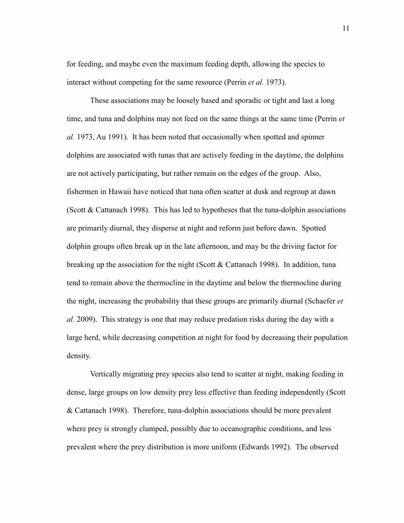
These associations may be loosely based and sporadic or tight and last a long
time, and tuna and dolphins may not feed on the same things at the same time (Perrin et
al. 1973, Au 1991). It has been noted that occasionally when spotted and spinner
dolphins are associated with tunas that are actively feeding in the daytime, the dolphins
are not actively participating, but rather remain on the edges of the group. Also,
fishermen in Hawaii have noticed that tuna often scatter at dusk and regroup at dawn
(Scott & Cattanach 1998). This has led to hypotheses that the tuna-dolphin associations
are primarily diurnal, they disperse at night and reform just before dawn. Spotted
dolphin groups often break up in the late afternoon, and may be the driving factor for
breaking up the association for the night (Scott & Cattanach 1998). In addition, tuna
tend to remain above the thermocline in the daytime and below the thermocline during
the night, increasing the probability that these groups are primarily diurnal (Schaefer et
al. 2009). This strategy is one that may reduce predation risks during the day with a
large herd, while decreasing competition at night for food by decreasing their population
density.
Vertically migrating prey species also tend to scatter at night, making feeding in
dense, large groups on low density prey less effective than feeding independently (Scott
& Cattanach 1998). Therefore, tuna-dolphin associations should be more prevalent
where prey is strongly clumped, possibly due to oceanographic conditions, and less
prevalent where the prey distribution is more uniform (Edwards 1992). The observed

12
12
associations are probably a time-varying combination of both tight groups and loosely
affiliated groups. The species may join and leave the groups in response to changes in
foraging situations. When the prey is clumped, they will forage together, when it is
dispersed, they forage independently. These groups may only last a few hours, or they
may last up to a few years (Au 1991).
The nature of these associations and which species takes the role of the leader
and the follower are both still unknown. In multispecies interactions, the more
behaviorally versatile species will often exploit the other species although there appears
to be some mutual benefits in this particular case (Au 1991). Some argue that it would
probably be disadvantageous for dolphins to follow tuna searching for food due to
dolphins' superior ability to find distant food via echolocation (Edwards 1992, Silva et
al. 2002). It has also been shown that tuna seek out dolphins of a particular size range,
those that travel approximately 100-130 cm/second. Large, mature yellowfin tuna travel
at an average speed of 120 cm/second, so finding these smaller dolphins to travel with
would not require the tuna to lose speed by slowing down, or energy by speeding up
(Edwards 1992). For this reason, the larger tuna would follow the smaller dolphins in
order to locate food patches more efficiently (Silva et al. 2002).
Purpose and Hypotheses
The purpose of this study is to investigate the presence of tuna-dolphin-bird
feeding assemblages in the Galapagos Marine Reserve using physical in situ data to
further characterize the habitat of these groups along with other cetacean and bird-tuna

13
13
groups. The objectives are to:
1.) Collect and review information already known on tuna-dolphin-bird
assemblages in the Eastern Tropical Pacific and specifically in the Galapagos
Marine Reserve;
2.) Characterize the upper 50 m of the water column using in situ data collected
via a hand-deployed CTD in areas of cetacean and bird-tuna sightings along
with areas of no sightings;
3.) Determine the relationship, if any, of the tuna-dolphin-bird assemblages,
cetacean groups, and bird-tuna assemblages to the strength and depth of the
thermocline.
The null hypotheses for this study are:
1.) Areas within in the Galapagos Marine Reserve will show no difference in
upper water column properties.
2.) There will be no difference in thermocline properties in areas where there are
tuna-dolphin-bird assemblages compared to areas where there are just bird-
tuna assemblages, cetacean groups, or no sightings.

14
14
CHAPTER II
PHYSICAL PROPERTIES OF THE SURFACE WATERS IN THE GALAPAGOS
MARINE RESERVE AND SURROUNDING AREA
The Galapagos Marine Reserve
The Galapagos Marine Resources Reserve (GMR) was established by the
Ecuadorian government in 1986 to protect the marine diversity that can be found around
the already established terrestrial Galapagos National Park (GNP). In area, it extends 40
nautical miles outside of a baseline drawn from the outermost points of the Galapagos
Archipelago (Jennings et al. 1994). This area is considered a biological “hot spot”
despite its position in the Equatorial Pacific Ocean, an area typically characterized by
high-nutrient low chlorophyll (HNLC) waters and low biological productivity.
This low productivity, despite the high nutrient concentrations, is due to iron
limitation; iron is a necessary ion for chlorophyll's structure (Palacios 2004). Typically,
the tropical waters around the Equator are well stratified with very low nutrient
concentrations. However, west of the archipelago, the Equatorial Undercurrent (EUC)
collides with the islands of Fernandina and Isabela, upwelling cold, nutrient rich water
(Sweet et al. 2007). In addition, iron is provided to the waters from the island platform
(Palacios 2004). This gives the Galapagos Islands a distinction as an “oasis” of
phytoplankton in an otherwise chlorophyll poor area. This, in turn, leads to the
congregation of marine species of all trophic levels around the archipelago, including
high trophic level and apex predators such as sharks, cetaceans, and marine pinnipeds
(Palacios 2004, Palacios et al. 2006, Sweet et al. 2007, Alva 2009).

15
15
North of the archipelago, the warmer tropical waters of the Panama Current
(PaC) approach the archipelago, creating a transition zone clockwise through the islands
as the water transitions from the warm tropical waters of the north to the cold upwelling
waters of the west (Fig. 3). These waters combine to form the weakly flowing South
Equatorial Current (SEC) that flows westward across the archipelago occupying the
surface waters up to depths of 20-50 m below the sea surface, depending on the season
(Sweet et al. 2007).
Figure 3. Schematic of major surface and subsurface currents impacting the Galapagos Islands. SEC =
Southern Equatorial Current; EUC = Equatorial Undercurrent; PaC = Panama Current; PC = Peru Current.
Solid lines indicate surface flows, dashed lines indicate subsurface flows, and arrows indicate primary
direction of flow. Adapted from Palacios (2004).
Due to this clockwise transition zone within the islands, the physical
characteristics of the water vary considerably throughout the archipelago. In addition,
16
16
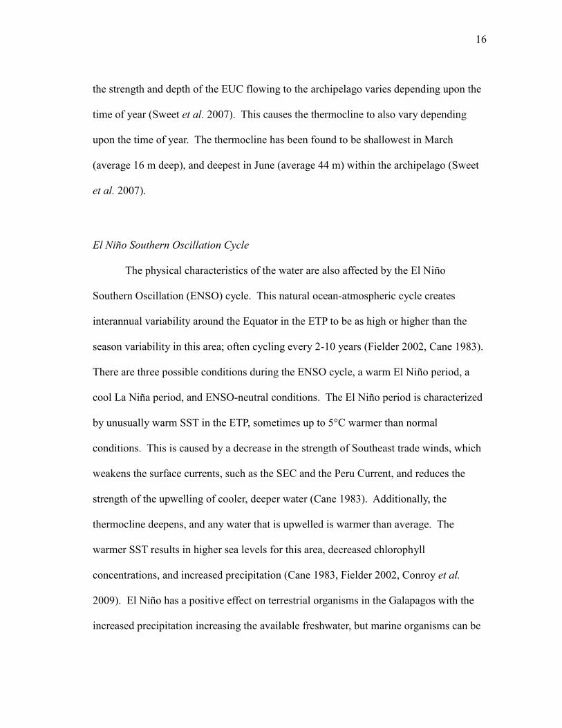
the strength and depth of the EUC flowing to the archipelago varies depending upon the
time of year (Sweet et al. 2007). This causes the thermocline to also vary depending
upon the time of year. The thermocline has been found to be shallowest in March
(average 16 m deep), and deepest in June (average 44 m) within the archipelago (Sweet
et al. 2007).
El Niño Southern Oscillation Cycle
The physical characteristics of the water are also affected by the El Niño
Southern Oscillation (ENSO) cycle. This natural ocean-atmospheric cycle creates
interannual variability around the Equator in the ETP to be as high or higher than the
season variability in this area; often cycling every 2-10 years (Fielder 2002, Cane 1983).
There are three possible conditions during the ENSO cycle, a warm El Niño period, a
cool La Niña period, and ENSO-neutral conditions. The El Niño period is characterized
by unusually warm SST in the ETP, sometimes up to 5°C warmer than normal
conditions. This is caused by a decrease in the strength of Southeast trade winds, which
weakens the surface currents, such as the SEC and the Peru Current, and reduces the
strength of the upwelling of cooler, deeper water (Cane 1983). Additionally, the
thermocline deepens, and any water that is upwelled is warmer than average. The
warmer SST results in higher sea levels for this area, decreased chlorophyll
concentrations, and increased precipitation (Cane 1983, Fielder 2002, Conroy et al.
2009). El Niño has a positive effect on terrestrial organisms in the Galapagos with the
increased precipitation increasing the available freshwater, but marine organisms can be
17
17
severely negatively affected, with little food available mass mortality can occur (Conroy
et al. 2009).
La Niña is characterized by opposite conditions. Southeast trade winds are
stronger than average, the thermocline is shallow, SST are cooler than average, and
upwelling is enhanced, resulting in higher chlorophyll concentrations. La Niña has a
positive effect on marine species, with plentiful food, but terrestrial species must endure
a drought, often resulting in negative effects on those species (Fielder 2002).
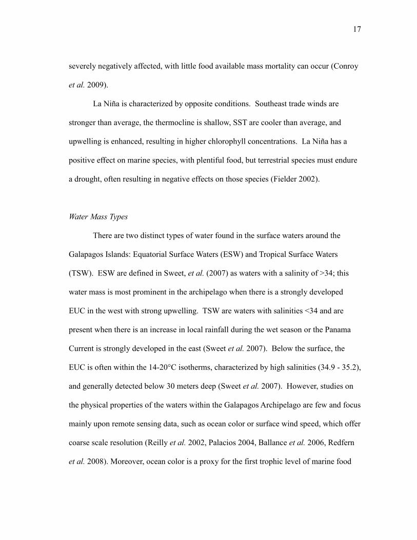
Water Mass Types
There are two distinct types of water found in the surface waters around the
Galapagos Islands: Equatorial Surface Waters (ESW) and Tropical Surface Waters
(TSW). ESW are defined in Sweet, et al. (2007) as waters with a salinity of >34; this
water mass is most prominent in the archipelago when there is a strongly developed
EUC in the west with strong upwelling. TSW are waters with salinities <34 and are
present when there is an increase in local rainfall during the wet season or the Panama
Current is strongly developed in the east (Sweet et al. 2007). Below the surface, the
EUC is often within the 14-20°C isotherms, characterized by high salinities (34.9 - 35.2),
and generally detected below 30 meters deep (Sweet et al. 2007). However, studies on
the physical properties of the waters within the Galapagos Archipelago are few and focus
mainly upon remote sensing data, such as ocean color or surface wind speed, which offer
coarse scale resolution (Reilly et al. 2002, Palacios 2004, Ballance et al. 2006, Redfern
et al. 2008). Moreover, ocean color is a proxy for the first trophic level of marine food

18
18
webs, primary production. Fine scale resolution investigations of the Galapagos are
important in determining the large amount of variability that occurs within the
Galapagos on seasonal, annual, and inter-annual time scales.
Survey Methods
Marine mammal surveys were completed in the southern part of the Galapagos
Islands during two weeks in June 2010. From June 4-6, observers recorded marine
mammal, sea turtle, and bird-fish assemblages between Puerto Ayora, Isla Santa Cruz,
Isla Floreana, and Puerto Villamil, Isla Isabela. Observers stood on the captain's pit on
the top of a 50ft fishing vessel called Lancha Cucaracha. At each tuna-bird-dolphin
assemblage, bird-tuna group, and dolphin group sighting a CTD was taken shortly after
the sighting in the vicinity of the sighting location. In addition, “non-sighting” CTD
data were collected as a control. CTDs were taken using a Sun and Sea Technology
CTD M48 Memory Probe. It was hand-deployed to depths between 12-35 meters.
Depths were estimated at time of collection based upon the amount of line released,
however strong currents often pulled the lightweight CTD horizontal rather than vertical,
often resulting shallower drops than anticipated. Temperature, conductivity, and
pressure were recorded four times a second and data were downloaded to Sun and Sea
Technology's Standard Data Acquisition software (SST-SDA) to determine drop depth
each evening and the amount of line released was modified to obtain drops of at least 20
meters of depth. A total of 6 drops were made during the 3-day survey. An INOCAR
officer recorded the survey track on-board using the GPS/laptop system HYPACK 2.0
19
19
and ArcGIS software 9.2.
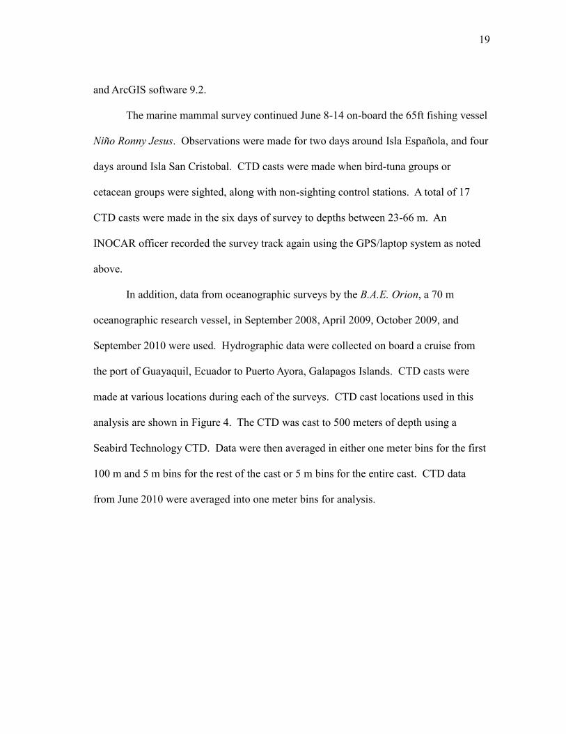
The marine mammal survey continued June 8-14 on-board the 65ft fishing vessel
Niño Ronny Jesus. Observations were made for two days around Isla Española, and four
days around Isla San Cristobal. CTD casts were made when bird-tuna groups or
cetacean groups were sighted, along with non-sighting control stations. A total of 17
CTD casts were made in the six days of survey to depths between 23-66 m. An
INOCAR officer recorded the survey track again using the GPS/laptop system as noted
above.
In addition, data from oceanographic surveys by the B.A.E. Orion, a 70 m
oceanographic research vessel, in September 2008, April 2009, October 2009, and
September 2010 were used. Hydrographic data were collected on board a cruise from
the port of Guayaquil, Ecuador to Puerto Ayora, Galapagos Islands. CTD casts were
made at various locations during each of the surveys. CTD cast locations used in this
analysis are shown in Figure 4. The CTD was cast to 500 meters of depth using a
Seabird Technology CTD. Data were then averaged in either one meter bins for the first
100 m and 5 m bins for the rest of the cast or 5 m bins for the entire cast. CTD data
from June 2010 were averaged into one meter bins for analysis.
20
20
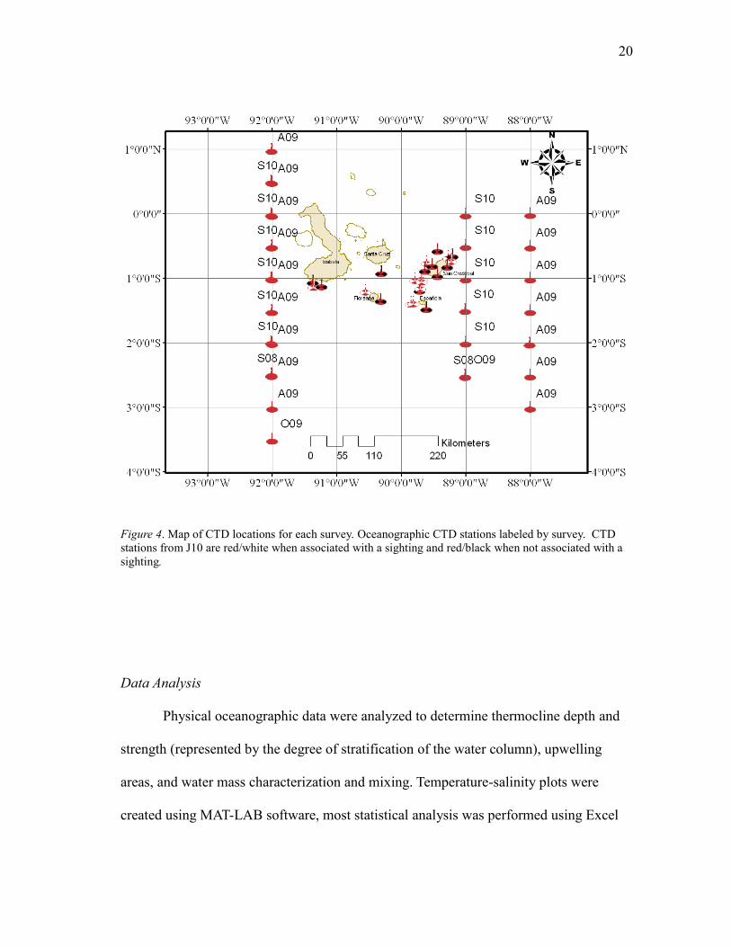
Figure 4. Map of CTD locations for each survey. Oceanographic CTD stations labeled by survey. CTD
stations from J10 are red/white when associated with a sighting and red/black when not associated with a
sighting.
Data Analysis
Physical oceanographic data were analyzed to determine thermocline depth and
strength (represented by the degree of stratification of the water column), upwelling
areas, and water mass characterization and mixing. Temperature-salinity plots were
created using MAT-LAB software, most statistical analysis was performed using Excel

21
21
2007 ©. For simplicity, surveys are labeled by the first letter of the month in which they
occurred, and the last two digits of the years (Table 1). ENSO cycle conditions were
determined based upon NOAA ENSO indices for Regions 1&2 (Figs. 5 & 6), which
have been show to correlate with SST around the Galapagos Islands (Conroy et al.
2009). Conditions for each survey are also listed in Table 1.
Table 1. Abbreviations for survey names and ENSO conditions during each of the surveys in this study.
Survey Label ENSO Conditions
September 2008 S08 Weak El Niño
April 2009 A09 Weak El Niño/Neutral
October 2009 O09 Moderate La Niña
June 2010 J10 Transition/Weak La Niña
September 2010 S10 Strong La Niña

22
22
Water masses were determined using modified definitions by Sweet, et al.
(2007), as described above. TSW and ESW were temperature independent, however
EUC only included water warmer than 14°C. Any water colder than 14°C was referred
to as “deepwater” (DW). Upwelling areas were defined as areas where Equatorial
Undercurrent Water was present at the sea surface.
Thermocline depths were determined by estimating the depth of the 20°C
isotherm (Donguy & Meyers 1987, Kessler 1990, Kessler et al. 1995, Fiedler 2010).
This method has been compared to Wyrtki’s (1964) method of determining the
thermocline boundaries based on a temperature change of greater than 0.3°C/10 m with
the thermocline depth defined as the depth with greatest temperature change and has
resulted in approximately similar depths (two tailed t-test assuming unequal variances, t
= 1.28, p = 0.20). Therefore for this study, the depth of the 20°C isotherm is the depth of
the thermocline. The stratification of the water column was represented by the greatest
change in temperature in °C per meter of depth (dt/dz). Drops with dt/dz less than
0.04°C/meter were given a stratification value of 0 (Palacios et al. 2004, Fiedler 2010).

23
23
S08 Box 2
Box 3
A09 O09
Figure 5. Time series of area-averaged sea surface temperature (SST) anomalies (°C) in the Niño regions: Niño-1+2 (0°-10°S, 90°W-80°W), Niño 3
(5°N-5°S, 150°W-90°W) for each survey. SST anomalies are departures from the 1971-2000 base period weekly means (CPC/NWS 2011).
J10 S10

24
24
Figure 6. SST anomalies (in °C) in the Equatorial Pacific during each survey: a.) S08; b.) A09; c.) O09; d.) J10; e.) S10 (CPC/NWS 2011).
b.) a.)
c.)
e.)
c.) d.)

25
25
Figure 6 Continued.
e.)

26
Results
All three major water masses in the Eastern Equatorial Pacific are found within
the Galapagos Archipelago throughout the survey based upon the sea surface salinities
(SSS). The temperature-salinity plot shows the distribution, and any mixing along
isopycnals, of the water masses within all the CTD from the surveys (Fig. 7). SSS
ranged between 33.1 and 35.6 with an average salinity of 34.7 (sd = 0.4) over all the
surveys (Fig. 8).
Figure 7. T-S plot of oceanographic CTD data and CTD data from the small boat survey in June 2010.
TSW is green, ESW is red, EUC is light blue, and DW is dark blue.
TSW
ESW
EUC
27
27
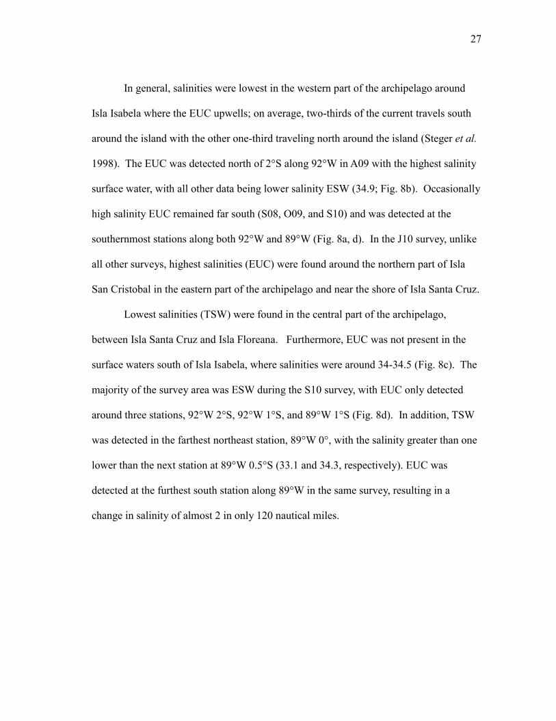
In general, salinities were lowest in the western part of the archipelago around
Isla Isabela where the EUC upwells; on average, two-thirds of the current travels south
around the island with the other one-third traveling north around the island (Steger et al.
1998). The EUC was detected north of 2°S along 92°W in A09 with the highest salinity
surface water, with all other data being lower salinity ESW (34.9; Fig. 8b). Occasionally
high salinity EUC remained far south (S08, O09, and S10) and was detected at the
southernmost stations along both 92°W and 89°W (Fig. 8a, d). In the J10 survey, unlike
all other surveys, highest salinities (EUC) were found around the northern part of Isla
San Cristobal in the eastern part of the archipelago and near the shore of Isla Santa Cruz.
Lowest salinities (TSW) were found in the central part of the archipelago,
between Isla Santa Cruz and Isla Floreana. Furthermore, EUC was not present in the
surface waters south of Isla Isabela, where salinities were around 34-34.5 (Fig. 8c). The
majority of the survey area was ESW during the S10 survey, with EUC only detected
around three stations, 92°W 2°S, 92°W 1°S, and 89°W 1°S (Fig. 8d). In addition, TSW
was detected in the farthest northeast station, 89°W 0°, with the salinity greater than one
lower than the next station at 89°W 0.5°S (33.1 and 34.3, respectively). EUC was
detected at the furthest south station along 89°W in the same survey, resulting in a
change in salinity of almost 2 in only 120 nautical miles.

28
28
a.)
b.)
Figure 8. Water mass types with salinity values for each of the five surveys: a.) S08 and O09, b.) A09, c.)
J10, d.) S10. Dot color signifies water type: blue = ESW, yellow = EUC, red = TSW; Labels denote SSS.

29
29
c.)
d.)
Figure 8. Continued.
30
30
a.)
b.)
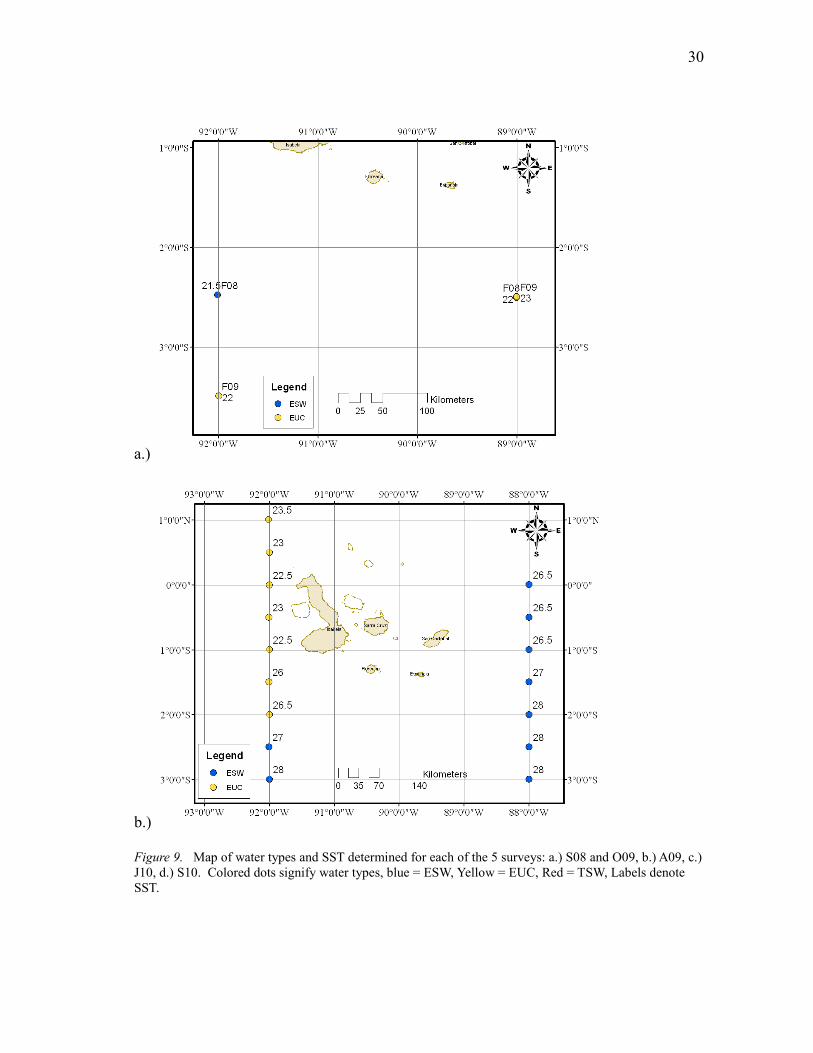
Figure 9. Map of water types and SST determined for each of the 5 surveys: a.) S08 and O09, b.) A09, c.)
J10, d.) S10. Colored dots signify water types, blue = ESW, Yellow = EUC, Red = TSW, Labels denote
SST.

31
31
c.)
d.)
Figure 9. Continued.

32
32
SST varied between 17°C and 28°C with an average temperature of 22.9°C (sd =
2.6) throughout the surveys (Fig. 9). In general, temperatures were warmest in the
eastern part of the archipelago and coldest west of Isla Isabela. In A09, temperatures
were coldest around Isla Isabela, but warmed south of 2°S (Fig. 9b). The colder waters
corresponded to lower salinities shown by the EUC upwelling in that region. East of the
archipelago, SST were the warmest recorded in this study; however they were still
primarily higher salinity ESW. SST were warmest in the center of the archipelago in
J10, with cooler temperatures in the east around Isla Española and Isla San Cristobal, in
the west around Isla Isabela, and along the coast of Isla Santa Cruz (Fig. 9c). These
warmer waters corresponded with the lower salinity TSW, whereas the cooler
temperatures were primarily ESW and EUC. The coldest SST recorded were in the S10
survey (Fig. 9d). Both the east and west areas of the archipelago had cooler waters than
even those found four months earlier in the J10 survey. Warm water was only found in
the far northeastern part of the survey where SST was warm (24°C) and was classified as
TSW.
The depth of the thermocline was on average 33 m deep (sd = 15 m) with a
maximum measured depth of 50 m. Three of the sites within the archipelago in the J10
survey have a thermocline deeper than the depth of the CTD cast: site 2-2 >13 m, site 3-
3 >16 m, and site 8-1 >44 m (Table 2). In addition, at site 4-4, the cast was in a shallow
area (25 m depth) and reached the bottom. The entire drop was well mixed and did not
have a thermocline and is labeled N/A. Thermoclines near Isla Isabela were generally
shallowest with the deepest thermocline depths around Isla San Cristobal. Thermocline

33
33
depths from the oceanographic surveys show deeper thermoclines in A09 and very
shallow in S10. Many of the sites in S10 had water colder than 20°C at the surface, and
are noted as NP in Table 2. The stratification of the water was strongest around the
northern tip of Isla San Cristobal and weakest around Isla Española. Dz/dt labeled with
ND were casts where the thermocline was deeper than the depth of the cast or the
thermocline was at the bottom of the cast and there were not sufficient data to accurately
determine the full area of the thermocline. Drops where the depth of the thermocline
was deeper than the maximum depth of the drop were labeled N/A, indicating
insufficient data available. In the oceanographic surveys, the stratification of the water
was generally weakest along 92°W and strongest along 89°W. An exception is between
0.5°N and 0.5°S along 92°W in the S10 survey, which had strongly stratified waters,
while no thermocline was recorded for the remainder of the sites along that longitude
and the waters were weakly stratified. Thermocline depth and thermocline strength
were poorly correlated (R2 = 0.017).

34
34
Table 2. Thermocline depth and stratification of the water column for each CTD cast.
Station Depth of 20°C Isotherm (m) dz/dt
June 2010
Isla Isabela
2-1 9 0.32
2-2 +13 N/A
2-3 14 0.56
Isla Floreana/Isla Santa Cruz
3-1 13 1.02
3-2 31 1.86
3-3 +16 N/A
Isla Espanola
5-1 23 1.26
5-2 13 0.45
5-3 33 0.41
6-1 30 0.26
6-2 31 0.75
6-3 39 0.51
6-4 24 0.34
Isla San Cristobal
4-1 30 0.78
4-2 N/A 0
7-1 15 0.69
7-2 40 0.28
7-3 19 0.65
7-4 20 1.52
8-1 +44 N/A
8-2 30 0.65
9-1 42 1.69
9-2 37 3.52
Oceanographic Cruises
September 2008
-89°W -2.5°S 40 0.27
-92°W -2.5°S 30 0.33
October 2009
-89°W -3.5°S 49 0.73
-92°W -3.5°S 32 0.33
April 2009
-88°W 0° 40 0.47
-88°W -0.5°S 50 0.31
35
35
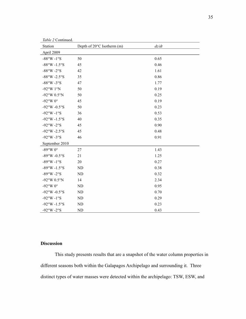
Table 2 Continued.
Station Depth of 20°C Isotherm (m) dz/dt
April 2009
-88°W -1°S 50 0.65
-88°W -1.5°S 45 0.46
-88°W -2°S 42 1.61
-88°W -2.5°S 35 0.86
-88°W -3°S 47 1.77
-92°W 1°N 50 0.19
-92°W 0.5°N 50 0.25
-92°W 0° 45 0.19
-92°W -0.5°S 50 0.23
-92°W -1°S 36 0.53
-92°W -1.5°S 40 0.35
-92°W -2°S 45 0.90
-92°W -2.5°S 45 0.48
-92°W -3°S 46 0.91
September 2010
-89°W 0° 27 1.43
-89°W -0.5°S 21 1.25
-89°W -1°S 20 0.27
-89°W -1.5°S ND 0.38
-89°W -2°S ND 0.32
-92°W 0.5°N 14 2.34
-92°W 0° ND 0.95
-92°W -0.5°S ND 0.70
-92°W -1°S ND 0.29
-92°W -1.5°S ND 0.23
-92°W -2°S ND 0.43
Discussion
This study presents results that are a snapshot of the water column properties in
different seasons both within the Galapagos Archipelago and surrounding it. Three
distinct types of water masses were detected within the archipelago: TSW, ESW, and

36
36
EUC. While the definitions of these water masses were based on salinities alone, the
temperature of the water also tended to correspond with the types of water mass (Wyrtki
1966, Sweet et al. 2007). TSW is low salinity water from the Panama Current which
flows south, turning slightly west near the Equator from Central America (Palacios
2004). The Panama Current reaches the Galapagos seasonally, from February to April,
when the Equatorial Countercurrent (ECC) and Peru Current (PC) are relatively weak
(Wyrtki 1966). TSW was found in the interior of the archipelago during the Garuá
season (J10), however, it was also detected along the Equator in the S10 survey, when
the ECC and SEC are strong.
This anomaly can be accounted for by the Equatorial Front (EF). The EF
separates the tropical water (TSW) characterized by high temperatures and low salinity
in the north from the cooler higher salinity water in the south, the ESW (see the
appendix for regional maps showing the EF). This front is strong during May to
November, and begins along the Peruvian coastline around 4°S, cuts across the Equator
east of the Galapagos, and continues north of the Equator throughout the remainder of
the Pacific Ocean (Wyrtki 1966). This front is also characterized by large horizontal
temperature and salinity differences, like those we see along 89°S in S10. Steger et al.
(1998) also found the EF along 89°W in November 1993. During a survey along 89°W
and 92°W with normal sea surface conditions, Steger noted that SST was 3°C warmer
and SSS was 1 greater at 1°N compared to 2°S. These values are similar to those in the
A09 survey, with SST 5°C warmer and SSS 2 greater at the Equator compared to 2°S.
These changes in values are indicative of the EF’s presence slightly below the Equator

37
37
east of the archipelago (Steger et al. 1998).
Both the sea surface temperature and salinities were somewhat anomalous in the
J10 survey. Salinities were lower than expected and temperatures higher than expected
around Isla Isabela, with opposite conditions around Isla San Cristobal. The high
salinities around Isla San Cristobal indicate that there may be some kind of localized
upwelling in the region. To support this, there were high chlorophyll concentrations to
the northwest of Isla San Cristobal at the time of the survey (Fig. 10). Additionally,
strong surface currents were observed around this area, indicating that a current may be
upwelling due to topographic blockage from the island. This would bring nutrients to
the surface, accounting for the high salinity, lower temperatures, and high chlorophyll
concentrations in the area. However, the strong and deep thermoclines in the northern
part of Isla San Cristobal surveyed suggest this upwelling maybe occurring downstream
of the area with the horizontal transport of nutrients. It is well documented that primary
productivity is enhanced around islands, an effect called the “island mass effect”
(Hasegawa et al. 2004, Hasegawa et al. 2009). It has been shown in the Western Pacific
Ocean that islands with deep waters around them often have high primary productivity
around them due to a variety of processes. These include the formation of eddies that
occur on the lee side of the island and cause localized upwelling that contributed
deepwater nutrients to the surface waters around the island (Hasegawa et al. 2004,
Hasegawa et al. 2009). This water can then be transported horizontally through the
surface currents (Gargett 1991).
The upwelling in these eddies can be seen as areas of low sea surface heights

38
38
compared to the rest of the area (Espinosa-Carreon et al. 2004). In Figure 10 an area of
low sea surface height (SSH) is present between Isla Santa Cruz and Isla San Cristobal,
suggesting the presence of a small eddy from the island mass effect of the SEC flowing
around Isla San Cristobal from the east to the west. However, caution must be used
when drawing conclusions from this figure; the composite is an optical interpolation of
eight days of data with resolution on an x-y scale of only about 100 kilometers. Though
an area of low SSH is indicated, the geometry of the low SSH region shown in Fig 10
is an interpolation. A monthly composite shows that there is a persistent area of high
productivity in the lee of Isla San Cristobal, with respect to the SEC (Fig. 11).
Figure 10. 8-day composite of chlorophyll concentrations around the Galapagos Islands, centered on June
5, 2010. Sea surface height contours (5cm) show positive anomalies with solid lines and negative
anomalies with dashed lines.

39
39
Figure 11. Monthly composite for June 2010 for chlorophyll concentrations around the Galapagos Islands.
Sweet et al. (2007) did a hydrographic survey around the Galapagos Islands in
2005-2006, with similar data collected (Morrison et al. 2009). One of the three surveys
occurs in the same month as the survey in this study, a June 2006 survey. In the current
study, thermocline depths were relatively shallow, less than 40 m, and shallowest in the
west while deepening eastward. However, Sweet found deep thermoclines throughout
the archipelago (>50 m) with the shallowest areas in the central archipelago rather than a
west to east gradient. Interestingly, the T-S plots from each of the surveys are similar;
both studies show there is very little TSW within the archipelago during this month and
the area is covered primarily by ESW. The most probable reason for the deeper

40
40
thermocline depths in J10 than in June 2006 is the ENSO cycle. June 2006 was
characterized by SST anomalies between +0.2 to +0.3°C above normal as an El Niño
began to develop, which caused a deepening of the thermocline and warmer SST with
relatively constant SSS. June 2010 was a transition period between an El Niño and a La
Niña with temperature anomalies -0.2 to -0.6°C below normal (Figs. 5 & 6). This period
was between a moderate El Niño in October 2009-Spring 2010 to a moderately strong
La Niña, through September 2010 (CPC/NWS 2011). This accounts for the differences
in thermocline depths and the similar salinities between the two surveys.
Additionally, the ENSO cycle likely accounts for the large variation in SST
between the A09 and S10 surveys. A09, with ENSO-neutral conditions, has SST up to
10°C greater than those in S10, with moderate La Niña conditions. SSS were also up to
1 greater in A09, than during the La Niña in S10. The sea surface conditions found in
A09 along 92°W are similar to those found in November 1993 by Steger et al. (1998), a
time of neutral sea surface conditions as well. Steger noted the EUC core around 0.5°S,
indicated by the coolest SST (19.5°C) and highest SSS (34.9). The EUC at this time was
turning predominately northeast, although high temperature and low salinity waters
(25.2°C and 33.8, respectively) were measured north of the Equator. In this study,
however, warmest temperatures were recorded south of the Equator, between 2°S and
3°S. SST were coolest between 1°S and the Equator which, along with high SSS,
indicates near surface EUC upwelling. It is important to note that the patterns in our
A09 survey and Steger’s November 1993 survey do not completely overlap. This is
probably due to the seasonal variations between the Garuá season (May – November)

41
41
and the wet season (December-April). During the Garuá season, upwelling is enhanced,
with cooler SST throughout the archipelago due to the Inter-tropical Convergence Zone
(ITCZ) reaching its northern most position. The wet season has warmer SST coinciding
with decreased upwelling and the ITCZ is near the Equator (Sweet et al. 2007). This
likely accounts for the differences in SST and SSS between Steger’s November 1993
survey and our A09 survey.

42
42
CHAPTER III
RELATIONSHIP OF TUNA-DOLPHIN-BIRD DISTRIBUTIONS
TO THE VARIABILITY OF WATER CONDITIONS IN THE ETP
Introduction
Tuna-dolphin-bird groups are unique the Eastern Tropical Pacific (ETP), an area
that includes everything from the western coast of the Americas to approximately 140°W
and between 20°N and 20°S (Edwards 1992). These associations are apparently a result
of the unique oceanographic features seen in this area (Au & Perryman 1985, Au 1991,
Ballance et al. 2006). Only in areas where the preferred habitats of yellowfin tuna and
their associated dolphins (common, striped, spotted or spinner) overlap in the ETP,
however, might one expect to find these mixed species groups of marine predators.
Therefore it is important to not only describe and analyze the oceanographic conditions
that are present in the Galapagos Islands, as in chapter two of this thesis, but also
determine how the distribution of tuna, dolphins, and seabirds are affected by those
oceanographic conditions.
Seasonal Variations in the Eastern Tropical Pacific
Since tuna tend to be more widespread than dolphins (Collette & Nauen 1983),
determining the dolphin habitat preferences allows us to locate tuna-dolphin
assemblages more easily. Smaller cetaceans do not typically undertake extensive pole
to pole migrations like the larger baleen species (Reilly 1990). Also, while dolphins can
change their distributions based on seasonal changes of water masses, there is little

43
43
seasonal change in the ETP, leading to little change in dolphin habitat (Reilly 1990). In
general, upwelling will supply nutrients to the upper water column, which occurs along
the equator, the countercurrent thermocline ridge, west of the Galapagos Islands, and
along the coast of South America. In the ETP, the thermocline is usually shallower in
the east and deepens westward. Also, the Equatorial Front (EF) is unstable and distorted
west of the Galapagos Islands due to high shear between the currents, but the EF is
generally better defined east of the Galapagos. The EF begins at the coast of Peru at
about 4°S, rising towards the equator as it reaches the Galapagos (Ballance et al. 2006).
The ETP in general is not often affected by strong seasonal changes, although the
area immediately around the Galapagos can experience strong seasonal variation (Sweet
et al. 2007). In addition, on the interannual scale, the El Niño-Southern Oscillation
(ENSO) cycle causes inter-annual and decadal changes in the water masses (Ballance et
al. 2006, Redfern et al. 2008). Since upwelling west of the Galapagos tends to be a
seasonal occurrence, seabirds and cetaceans will follow their preferred habitat conditions
as those conditions move spatially during the seasonal and interannual changes (Ballance
et al. 2006). Also, some coastal species of dolphins move in response to seasonal
movements of their prey, following their food source as it changes its distribution (Reilly
1990).
However, various features of the ETP can fluctuate in strength or prevalence and
are not all synchronized. The southeast trade winds, the Peru Current, and the Southern
Equatorial Current all change seasonally with weak periods during the winter and
strengthening during the summer (Fielder 2002). From July to December there is greater

44
44
equatorial upwelling and more horizontal transport in the Peru Current (Reilly 1990).
The Equatorial Cold Tongue is strongly developed from August through October;
however, it is weak from February to April (Ballance et al. 2006).
ENSO Cycle
The ENSO cycle is mainly responsible for the moderately strong inter-annual
variations in the ETP. This cycle causes marked changes in the “typical” oceanographic
conditions of the area. These changes are believed to affect prey densities, which in turn
would affect the density and distribution of their predators (Ballance et al. 2006, Redfern
et al. 2008). However, the relationship between the ENSO cycle's effect of
oceanographic conditions and the prey-predator interactions are not well understood
(Redfern et al. 2008). As mentioned previously, the warm cycle of ENSO, or El Niño,
results in significantly warmer sea surface temperatures (SST) and reduced upwelling,
causing the decrease in food availability due to resource limitation. The cold cycle, or
La Niña, increases the productivity of the oceans with enhanced upwelling, cold SST
and abundant food resources (Cane 1983, Fielder 2002).
Cetacean Habitat
Cetacean habitat is often defined by oceanographic variables; however, their
movements may not be directly related to these characteristics (Redfern et al. 2008).
Most studies use variables such as SST, SSS, and thermocline depth to determine areas
where cetaceans are more likely to be observed, or as a proxy for predicting where their

45
45
prey may be located. These physical variables are believed to influence prey availability
and density, thereby controlling where the cetaceans might aggregate (Redfern et al.
2008).
Since tuna are mainly associated with spotted, stripped, spinner, and common
dolphins, their preferred habitats are most important to finding tuna-dolphin
aggregations. Each species of dolphin seems to prefer general characteristics of habitat
that sometimes overlap between the species. The difference between habitat preferences
in each of these species of dolphins is probably not directly related to the physical
variables themselves, but rather the prey that reside in each of these areas (Ballance et al.
2006).
Common dolphins, along with pilot whales, bottlenose dolphins, Risso's
dolphins, and Bryde's whales prefer areas of upwelling. Food chains tend to be shorter
in upwelling modified waters, which usually results in common dolphins feeding low on
the food chain. Common dolphins tend to occupy the coldest, most saline waters of the
ETP: areas east and west of the Galapagos where they appear with striped dolphins (Au
& Perryman 1985, Wade & Gerrodette 1993, Reilly et al. 2002, Ballance et al. 2006).
Striped dolphins tend to be more widespread and usually aggregate in smaller
schools than common dolphins. They often inhabit the eastern boundary current's
coastal upwelling regions where they may occur as part of a mixed species group with
common dolphins (Ballance et al. 2006). In addition, stripped dolphins are typically
distributed where the other types of dolphins are not found (Wade & Gerrodette 1993,
Reilly et al. 2002) including areas where the water is shallow (<300 m), and where the

46
46
thermocline is strong and shallow (Redfern et al. 2008). Where common dolphins and
stripped dolphins occur as mixed groups, the ocean is usually characterized by highly
variable oceanographic features that are upwelling modified (Au & Perryman 1985).
This upwelling modified area has weak thermoclines, cool surface temperatures (<25ºC),
high salinities (>34.5), and high chlorophyll concentrations (Ballance et al. 2006,
Redfern et al. 2008). These mixed groups are frequently found along the equatorial
waters out to 100ºW, with higher abundances west of the Galapagos (Au & Perryman
1985, Reilly 1990).
Spotted dolphins are also found occasionally in the cooler, upwelling modified
waters, but generally they prefer areas with deep thermoclines (>70 m) (Reilly 1990).
Spotted dolphins often join schools of spinner dolphins, forming multispecies pods of
dolphins that can number in the thousands. These groups are most abundant in areas of
warm tropical waters with low salinities (<34), deep, sharp thermoclines (>2ºC/10 m),
strong water column stratification, very warm, stable surface water (>25ºC), and low
surface chlorophyll concentrations (Wade & Gerrodette 1993, Reilly 1990, Reilly et al.
2002, Ballance et al. 2006, Redfern et al. 2008). While common dolphin habitat is
centered on the equator, spotted/spinner groups are rarely observed near the equator (Au
& Perryman 1985). Instead, these groups live north and south of the equator, along the
warm edge of the Peru Current, and near the Costa Rica Dome (Au & Perryman 1985,
Reilly 1990, Ballance et al. 2006). They have low abundances between the South
American Coast and the Galapagos Islands (Reilly 1990).
47
47
Yellowfin Tuna Habitat
Also important in analyzing tuna-dolphin-bird distributions are the habitat
requirements of the yellowfin tuna. These tuna prefer areas with gradual thermocline
gradients that are shallow rather than a sharp, deep thermocline (Green 1967). Shallow
thermoclines along with areas of high chlorophyll concentrations can result in the
aggregation of a high abundance of potential prey, compared to areas with a deep
thermocline and low chlorophyll concentration (Ballance et al. 1997). These are areas
where the tuna prefer to feed, presumably because there is more food available.
Furthermore, the shallow thermocline may act as a vertical barrier and keep the
squid and fishes the dolphin and tuna prey upon from a quick escape to deeper water.
These areas allow successful foraging for both tuna and dolphins alike, and by keeping
the prey close to the surface, birds can join in the feeding frenzy (Reilly 1990). The O2
minimum zone is often close to the shallow thermocline and will also keep prey from
escaping to deeper water (Green 1967).
Most tuna tend to occupy the warmest water available; yellowfin tuna have
acclimated to the cooler surface temperature waters in the ETP compared to other
tropical waters. Tuna have the ability to maintain their body temperature higher than the
ambient water temperature; yellowfin tuna are often 1.4-4°C warmer than the
surrounding water (Block et al. 1997). Their depth distribution is determined by the
relative change in water temperature rather than a specific temperature (Brill et al. 1999,
Brill & Lutcavage 2001) and the depth of the oxygen minimum zone (Gooding et al.
1981). Yellowfin tuna are not found at depths where the temperature is more than 8°C

48
48
cooler than the surface waters for long periods of time, although they may dive deeper
occasionally. In areas where there is a very shallow thermocline, this constrains tuna to
the upper 20-30 meters of the water column where they are more likely to associate with
dolphins (Brill et al. 1999, Brill & Lutcavage 2001).
Bird Assemblage Distribution
The distribution of bird assemblages in the ETP is generally believed to be
influenced primarily by the environmental characteristics of the area, including water
mass types and current systems (Ribic & Ainley 1997). Additionally, these bird groups
can be found associated with these same characteristics regardless of the ENSO stage,
with ENSO events having very little impact on the distribution of these birds (Ribic &
Ainley 1997). Generally, storm petrels are associated with the ESW, following the SEC,
and shearwaters are associated with the warmer, low salinity TSW with deep
thermoclines. It has been suggested that the depth of the thermocline is an indicator for
the amount of productivity in an area. If this is the case, then areas of high productivity
may be a predictor for bird assemblage presence (Ribic & Ainley 1997). Bird
assemblages are found associated with tuna-dolphin groups primarily in the TSW, north
of 5°N, with the majority of the tuna-dolphin-bird groups between the Equator and 5°S
comprised of shearwaters and boobies (Au & Pitman 1988). Whenever TSW are within
the Galapagos, generally December through February, these bird assemblages can be
found associated with tuna-dolphin groups (Au & Pitman 1988).

49
49
Tuna-dolphin-bird Groups: Working Hypotheses
1.) In the Galapagos Marine Reserve, tuna-dolphin-bird groups would be found
where their respective habitats overlap, including around the western side of
the archipelago where there are upwelling modified waters with shallow,
gradual thermoclines and abundant food resources.
2.) These groups would also tend to form in the middle of the archipelago where
the cooler subsurface water is close to the sea surface and a shallow
thermocline with warm surface waters is predominant.
3.) There would be a greater occurrence of these groups during normal
conditions, rather than during El Niño with deep thermoclines or La Niña
with cold SST.
4.) The tuna in the GMR would associate with common and/or striped dolphins
which are most likely to be found around the Galapagos Islands.
Survey Methods
Marine Mammal Surveys
Marine mammal surveys were completed in the southern part of the Galapagos
Islands during two weeks in June 2010. From June 4-6, observers recorded marine
mammal, sea turtle, and bird-fish assemblages between Puerto Ayora, Isla Santa Cruz,
south and west to Puerto Villamil, Isla Isabela (Fig. 12). Observers stood on the captain's
pit on the top of a 50ft fishing vessel called Lancha Cucaracha. For each sighting the
position, time, species, and an estimate of abundance was recorded if the group was

50
50
close enough for observation. Photos were taken of each sighting to verify species
identities. Every half-hour the position, weather conditions, and sea state were recorded.
The sea state was a Beaufort 4 on average, making observation with 7x50 hand-held
binoculars difficult; therefore most observations were carried out with the naked eye.
The marine mammal survey continued June 8-14 on-board the 65ft fishing vessel
Niño Ronny Jesus. Observations were made for two days around Isla Española, and four
days around Isla San Cristobal. Two observers stood 30 minute watches, rotating with
two other observers resting. Observers used 7x50 hand-held binoculars while sitting in
the captain's pit. The recording observer recorded marine mammal, bird, and sea turtle
sighting data as described above, along with environmental conditions every 30 minutes.
In addition, data from oceanographic surveys by the B.A.E. Orion, a 70 m
oceanographic research vessel, in September 2008 (S08), April 2009 (A09), October
2009 (O09), and September 2010 (S10) were used. Marine mammal surveys were
conducted during daylight hours from the port of Guayaquil, Ecuador to Puerto Ayora,
Galapagos Islands (Fig. 12). Two to three observers were on watch for 30 minute
rotations, with the port observer watching from 0° at the bow to 90° to the port and the
starboard observer watching from 0° at the bow to 90° to the starboard. Surveys were
conducted using 7x50 binoculars and recording position, speed, ocean conditions, and
meteorological conditions every 30 minutes. The third observer, when available, served
as the note taker and watched for sea lions, sharks, and sea turtles in the waters directly
around the boat.

51
51
Figure 12. Approximate routes taken during oceanographic and small boat marine mammal surveys. Line
colors denote survey tracks as follows: Orange denotes S08; Green denotes O09; Red denotes A09; Black
denotes J10; Blue denotes S10.
Data Analysis
Maps of cetacean, bird, and tuna group sightings were plotted in ArcGIS software
9.2. Data were plotted for each cruise individually with identifying labels for tuna-
dolphin-bird groups, birds, single species cetacean groups, and multiple species
cetacean/cetacean or cetacean/pinniped groups. The range of yellowfin tuna was
determined by finding the depth at which there was a greater than 8°C difference in
temperature from the sea surface temperature (Brill et al. 1999). Statistical significance
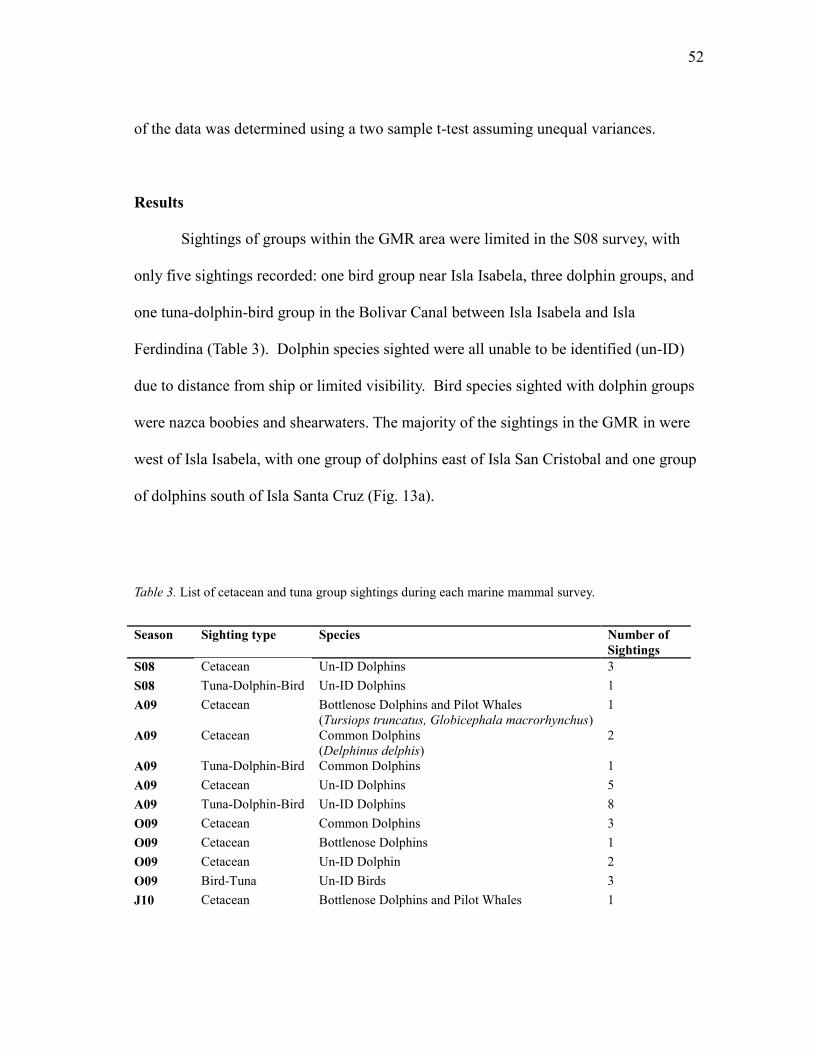
52
52
of the data was determined using a two sample t-test assuming unequal variances.
Results
Sightings of groups within the GMR area were limited in the S08 survey, with
only five sightings recorded: one bird group near Isla Isabela, three dolphin groups, and
one tuna-dolphin-bird group in the Bolivar Canal between Isla Isabela and Isla
Ferdindina (Table 3). Dolphin species sighted were all unable to be identified (un-ID)
due to distance from ship or limited visibility. Bird species sighted with dolphin groups
were nazca boobies and shearwaters. The majority of the sightings in the GMR in were
west of Isla Isabela, with one group of dolphins east of Isla San Cristobal and one group
of dolphins south of Isla Santa Cruz (Fig. 13a).
Table 3. List of cetacean and tuna group sightings during each marine mammal survey.
Season Sighting type Species Number of
Sightings
S08 Cetacean Un-ID Dolphins 3
S08 Tuna-Dolphin-Bird Un-ID Dolphins 1
A09 Cetacean Bottlenose Dolphins and Pilot Whales
(Tursiops truncatus, Globicephala macrorhynchus)
1
A09 Cetacean Common Dolphins
(Delphinus delphis)
2
A09 Tuna-Dolphin-Bird Common Dolphins 1
A09 Cetacean Un-ID Dolphins 5
A09 Tuna-Dolphin-Bird Un-ID Dolphins 8
O09 Cetacean Common Dolphins 3
O09 Cetacean Bottlenose Dolphins 1
O09 Cetacean Un-ID Dolphin 2
O09 Bird-Tuna Un-ID Birds 3
J10 Cetacean Bottlenose Dolphins and Pilot Whales 1

53
53
Out of 19 groups sighted in A09, nine were tuna-dolphin-bird groups with only
one group of positively identified species, the common dolphin. All of these groups
were sighted south of Isla Isabela near Isla Floreana. Additionally, there was one mixed
species group of bottlenose dolphins and pilot whales, two groups of common dolphins,
and five unidentified dolphin groups. Bird species were boobies (various species),
shearwaters, storm petrels (various species), and un-ID birds. There were only two
groups sighted south east of Isla Española, all other sightings were either west or south
of Isla Isabela (Fig. 13b).
Table 3 continued
Season Sighting type Species Number of
Sightings
J10 Cetacean Bottlenose dolphins and Sperm Whales
(T. truncates, Physter macrocephalus)
2
J10 Cetacean Common Dolphins 2
J10 Cetacean Bottlenose Dolphins 1
J10 Tuna-Dolphin-Bird Common Dolphins 1
J10 Cetacean Un-ID Dolphins 7
J10 Cetacean Whales (Various Species) 15
S10 Cetacean Bottlenose Dolphins 2
S10 Cetacean Common Dolphin 1
S10 Cetacean Striped Dolphin
(Stenella coeruleoalba)
1
S10 Cetacean Un-ID Dolphin 1
S10 Bird-Tuna Un-ID Birds 1

54
54
a.)
b.)
Figure 13. Distribution of groups sighted near the Galapagos (92°W-89°W and 0.5°N-2°S) from all the
oceanographic surveys: a.) S08, b.) A09, c.) O09, and d.) S10. Yellow birds represent bird group
sightings; blue dolphins represent single species dolphin groups; red fish represent tuna-dolphin-bird
group sightings. Sightings are labeled by the oceanographic survey during which they were sighted.

55
55
c.)
d.)
Figure 13. Continued.

56
56
There were a total of eight O09 groups sighted: three bird groups, three common
dolphin groups, one bottlenose dolphin group, and two groups of un-ID dolphins. Bird
species indentified included blue-footed and nazca boobies and shearwaters. Three of
these sightings were west of Isla Isabela, two were within the center of the archipelago
around Isla Floreana and Isla Santa Cruz, and four sightings were east of Isla San
Cristobal (Fig. 13c).
The 39 sightings in J10 included 15 whale species, one group of common
dolphins, one bottlenose dolphin group, and seven groups of un-ID dolphins.
Additionally, there were three mixed species groups, two of bottlenose dolphins and sea
lions and one of bottlenose dolphins and pilot whales, and one tuna-common dolphin-
bird group. The tuna-dolphin bird group was the only sighting south of Isla Isabela,
with the rest either between Isla Isabela, Isla Floreana, and Isla Santa Cruz or around Isla
San Cristobal and between Isla San Cristobal and Isla Española. There were no
sightings south and east of Isla Española, with the only sightings to the west (on two
different days) around a frontal boundary, an area marked with visible convergence or
divergence at the surface, where there were large groups of cetaceans sighted and large
groups of sea lions sighted (Fig. 14).
There were few sightings during the S09 survey, with only one bird group and
five cetacean sightings. Most of the sightings were around Isla San Cristobal, with three
of the sightings south of the island: two bottlenose groups and a common dolphin group.
There was one striped dolphin group and the bird group northeast of the island. The
only other cetacean sighting was west of Isla Isabela, un-ID dolphins (Fig. 13d).

57
57
Figure 14. Distribution of groups sighted from the J10 near shore survey around the Galapagos Islands.
Blue dolphins represent single species groups of dolphins; purple dolphins represent mixed species groups
of marine mammals (cetacean/cetacean or cetacean/pinnipeds); Green whales represent individual or
group whale sightings; red fish represent tuna-dolphin-bird assemblages; yellow birds represent bird
groups.
The maximum depth of the distribution of yellowfin tuna, referred to as their
vertical limit, around the Galapagos (88°W, 89°W, and 92°W) are shown in Figure 15.
General trends show a deepening of their vertical limit to the north in April 2009, a
deepening of their limit to the south in September 2010, and generally deeper vertical
limits along 92°W compared to 89/88°W. There were no significant differences between

58
58
depths for the pooled data 92°W and 88/89°W (Table 4). However, there were
significant differences between longitudes in September 2010 but not in April 2009.
There were also differences between pooled data from April 2009 and September 2010.
Data from September 2008 and October 2009 were not analyzed for significance due to
a small sample size. Data from June 2010 were not included in this analysis because
CTD casts were not deep enough to reach water 8°C colder than the surface temperature.
The maximum temperature difference recorded between the surface and bottom of cast
was 7°C, with an average temperature difference between the surface and bottom of cast
of 4°C.
Figure 15. Maximum depth of tuna distribution at each oceanographic CTD station based on a difference
of ≥8°C from SST. Circles represent stations along 88°W or 89°W (east of the archipelago); diamonds
represent stations along 92°W. Same color markers are from the same survey with orange markers from
S08, blue from A09, green from O09, and Red from S10.
0
50
100
150
200
250
300
350
400
450
-4 -3 -2 -1 0 1 2
De
pth
(m
)
Degree Latitude
Depth of 8°C Change
89W (S08)
88W (A09)
89W (O09)
89W (S10)
92W (S08)
92W (A09)
92W (O09)
92W (S10)
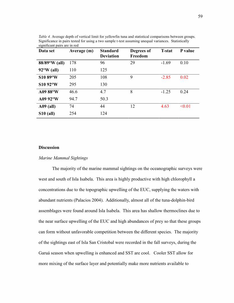
59
59
Table 4. Average depth of vertical limit for yellowfin tuna and statistical comparisons between groups.
Significance in pairs tested for using a two sample t-test assuming unequal variances. Statistically
significant pairs are in red
Data set Average (m) Standard
Deviation
Degrees of
Freedom
T-stat P value
88/89°W (all) 178 96 29 -1.69 0.10
92°W (all) 110 125
S10 89°W 205 108 9 -2.85 0.02
S10 92°W 295 130
A09 88°W 46.6 4.7 8 -1.25 0.24
A09 92°W 94.7 50.3
A09 (all) 74 44 12 4.63 <0.01
S10 (all) 254 124
Discussion
Marine Mammal Sightings
The majority of the marine mammal sightings on the oceanographic surveys were
west and south of Isla Isabela. This area is highly productive with high chlorophyll a
concentrations due to the topographic upwelling of the EUC, supplying the waters with
abundant nutrients (Palacios 2004). Additionally, almost all of the tuna-dolphin-bird
assemblages were found around Isla Isabela. This area has shallow thermoclines due to
the near surface upwelling of the EUC and high abundances of prey so that these groups
can form without unfavorable competition between the different species. The majority
of the sightings east of Isla San Cristobal were recorded in the fall surveys, during the
Garuá season when upwelling is enhanced and SST are cool. Cooler SST allow for
more mixing of the surface layer and potentially make more nutrients available to
60
60
support more prey for cetaceans. Tuna-dolphin-bird groups are less often present east of
the archipelago because of the deeper thermocline does not promote formation of these
groups (Au 1991).
Sightings were generally lower in the three fall surveys than the one spring
survey. The fewest sightings were recorded in the fall survey S08. The low number of
sightings in S08 can be attributed to the El Niño conditions that were present at this time.
El Niño has significant negative impacts on marine life due to the decrease in upwelling
and the low chlorophyll a concentrations, which cannot support the prey the marine
mammals rely upon (Cane 1983, Fielder 2002). The high number of sightings in A09
can be attributed to both the water conditions due to the ENSO cycle and the annual
season. The spring survey took place during the hot season, when SST are warm;
additionally, NOAA cites A09 as a weak El Niño/neutral conditions (CPC/NWS 2011).
The difference in the distribution of sightings between the spring and fall surveys may be
the result of the marine mammals adjusting their distribution to remain in the warmer
waters as the distribution of the warm water changes from the cooler Garuá season to the
warmer hot season. While not generally recorded, tuna may also change their
distribution to stay in the warmer surface waters in this area, accounting for the low
numbers of tuna groups seen in the fall surveys.
The one summer survey, J10, found opposite trends than those of the
oceanographic surveys. The majority of the sightings were around Isla San Cristobal,
with only a few recorded while in transit between Isla Santa Cruz and Isla Floreana and
between Isla Floreana and Isla Isabela. There was only one sighting south of Isla Isabela
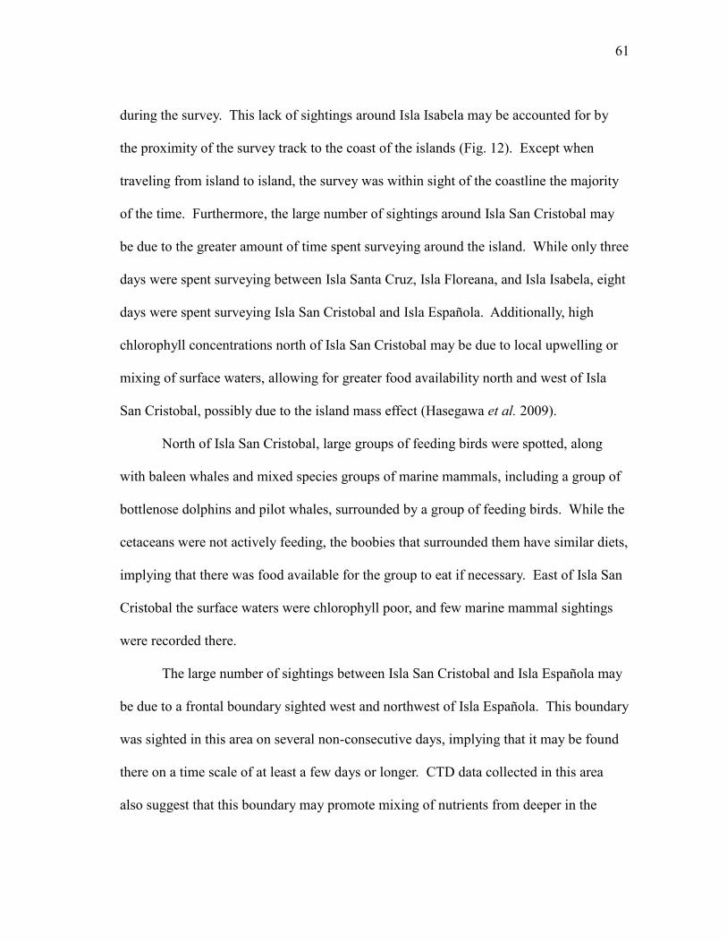
61
61
during the survey. This lack of sightings around Isla Isabela may be accounted for by
the proximity of the survey track to the coast of the islands (Fig. 12). Except when
traveling from island to island, the survey was within sight of the coastline the majority
of the time. Furthermore, the large number of sightings around Isla San Cristobal may
be due to the greater amount of time spent surveying around the island. While only three
days were spent surveying between Isla Santa Cruz, Isla Floreana, and Isla Isabela, eight
days were spent surveying Isla San Cristobal and Isla Española. Additionally, high
chlorophyll concentrations north of Isla San Cristobal may be due to local upwelling or
mixing of surface waters, allowing for greater food availability north and west of Isla
San Cristobal, possibly due to the island mass effect (Hasegawa et al. 2009).
North of Isla San Cristobal, large groups of feeding birds were spotted, along
with baleen whales and mixed species groups of marine mammals, including a group of
bottlenose dolphins and pilot whales, surrounded by a group of feeding birds. While the
cetaceans were not actively feeding, the boobies that surrounded them have similar diets,
implying that there was food available for the group to eat if necessary. East of Isla San
Cristobal the surface waters were chlorophyll poor, and few marine mammal sightings
were recorded there.
The large number of sightings between Isla San Cristobal and Isla Española may
be due to a frontal boundary sighted west and northwest of Isla Española. This boundary
was sighted in this area on several non-consecutive days, implying that it may be found
there on a time scale of at least a few days or longer. CTD data collected in this area
also suggest that this boundary may promote mixing of nutrients from deeper in the

62
62
water column, with lower SST and SSS east of the boundary than west of the boundary.
Along this boundary, large groups of sea lions (approx. 30-40 in one sighting) were
found jughandling, a behavior involving floating in the surface waters with one fore fin
grasped between their back fins, held out of the water, generally believed to be for body
temperature maintenance (Riedman 1990). Additionally, large groups of cetaceans were
spotted around the boundary, including a group 200-400 bottlenose dolphins and a group
of common dolphins.
Tuna Vertical Distribution
Yellowfin tuna have been found to be limited in their vertical distribution by a
temperature difference of 8°C colder than the surface temperature of the water,
regardless of the sea surface temperature (Brill et al. 1999, Brill & Lutcavage 2001).
Around the Galapagos Islands, this temperature difference is controlled significantly by
the upwelling of the EUC west of Isla Isabela. Where the EUC upwells, the SST will be
colder than elsewhere around the archipelago making the vertical limit of the tuna much
deeper because the colder deeper water is now at the surface. During the Garuá season,
when upwelling is enhanced and sea surface temperatures are cool, fewer aggregations
of tuna and dolphins were observed. Upwelling of the EUC occurs primarily around
92°W and the cold water tends to move north and south around Isla Isabela.
In all oceanographic cruises, the tuna’s vertical limit was significantly lower
along 92°W between 2°S and the equator, the main area influenced by the upwelling.
Along 88°W and 89°W, east of the archipelago, the vertical limit of the tuna is not as

63
63
much impacted by the upwelling, and the limit is much shallower than along 92°W.
However, when all data were pooled, there was no significant difference between the
two latitudes (Table 4). In general, we would expect to see more tuna dolphin
assemblages along the eastern side of the archipelago if their presence was due solely to
the vertical limitation by temperature and their distribution would change as the annual
season changes the water temperature. However, because we observed more groups
along 92°W, there may be additional influences on tuna distribution in the GMR.
The ENSO cycle conditions were different during each oceanographic survey,
and may help explain the changes in tuna-dolphin-bird distribution. For example, the
vertical limit is significantly shallower in April 2009 during ENSO-neutral conditions
than in September 2010 during a strong La Niña event. These neutral conditions had
slightly deeper 20°C isotherm depths, but warmer SST, making the depth at which there
is an 8°C difference in temperatures shallower than during the La Niña when the SST is
much cooler, at times less than 20°C, resulting in the increase in water depth needed to
reach the 8°C threshold. This is because the ENSO cycle generally only impacts the
upper 150-200 m of the water column in the ETP (Fielder 2002, CPC/NWS 2011) and
the water beneath this layer maintains its temperature structure of ENSO-neutral
conditions. Conditions in the archipelago during neutral conditions are favorable to the
formation of tuna-dolphin-bird groups, many of which were observed during the A09
survey. These groups formed due to the shallow and sharp thermoclines, forcing the
yellowfin tuna in the highly productive surface waters where the EUC shoals towards the
surface, bringing nutrient rich water into the photic zone.

64
64
The La Niña (S10) increased the difference in vertical limits between the eastern
and western side of the archipelago due to the increased upwelling and the greater extent
of the surfaced cold water along 92°W. More tuna-dolphin-bird groups were observed
throughout the archipelago during normal conditions and the hot season in A09 (nine
reported) than in any of the Garuá season and/or La Niña events (two tuna-dolphin-bird
groups and three bird-tuna groups reported, in total).
Additionally, in the summer survey, J10 a tuna-dolphin-bird group was spotted
south of Isla Isabela while several bird-tuna feeding assemblages were spotted around
Isla Española, south east of the archipelago. Since the J10 survey was during a transition
period between a strong El Niño and a strong La Niña, there were shallower
thermoclines across the entire archipelago, increasing the likelihood that where the tuna
fed close to the surface, dolphins and/or birds fed with them.
Most literature does not cite significant horizontal limits to the biogeographic
distribution of yellowfin tuna except that they are only found in tropical waters with
warm SST, generally between 18°C and 31°C (Collette & Nauen 1983). Obviously,
events such as ENSO events, which can change the SST in an area by several degrees,
may influence the horizontal distribution of the tuna. During the La Niña in S10, SST
along 92°W ranged from 22°C to 17°C, a difference of five degrees. The same CTD
stations during the A09 cruise had a SST range of 27 to 22°C. In only 18 months, the
temperature of the water varied by 10°C. Assuming the 8°C limit of the tuna’s
distribution, we would expect tuna to be horizontally restricted in their distributions on
an annual to interannual scale when the SST changes significantly in response to the

65
65
ENSO cycle.
Brill et al. (1999) and Brill and Lutcavage (2001) estimated the vertical
distribution of yellowfin tuna based on their movements in Hawaii, a tropical area with
little seasonal change in SST. Around the Galapagos, there are significant annual and
interannual changes in SST, making the horizontal changes in SST important to the
tuna’s distribution as well. This is not unexpected, though since many organisms
(pelagic cetaceans and seabirds in particular) are known to change their distributions in
response to the movement of water masses (Ballance et al. 2006). Similarly , it has
been shown that in the Eastern Pacific Ocean, yellowfin tuna will travel north and south
of the tropics as the subtropical water warms in the summer months and return to the
tropics as the water cools in the fall and winter months (Broadhead & Barrett 1964).
Tuna altering their distribution would be similar to the movement of those cetaceans,
resulting in less tuna-dolphin-bird groups present during the periods when SST were
cooler.

66
66
CHAPTER IV
CONCLUSIONS
Conclusions
There are distinct contrasts between the physical oceanographic characteristics of
the Galapagos Marine Reserve intra-annually (between the Garuá and hot seasons) and
inter-annually (between El Niño, La Niña, and ENSO-neutral periods). These changes
may affect the distribution of marine mammals and change the possibility of the
formation of tuna-dolphin-bird assemblages. The intra-annual changes within the GMR
occur when warm SST, high rainfall, and low salinities during the hot season shift to
cooler SST, enhanced upwelling, higher SSS, and low rainfall during the Garuá season
(Sweet et al. 2007). The lower frequency interannual changes can disrupt this cycle to
cause abnormally warm SST and suppression of upwelling during El Niño events, to
enhanced upwelling with abnormally cool SST during La Niña events (Fielder 2002).
Intra- and interannual cycles combine to create a unique environment around the
Galapagos Islands.
These changes in the physical characteristics of the water column in the GMR are
much stronger than in other parts of the ETP where the major factor in changes is the
ENSO cycle and there are only small annual changes. It is believed that marine
mammals adjust their distribution to compensate for the changes in the water properties
(Ballance et al. 2006) and that they generally follow their preferred habitat as it changes
spatially throughout the year in response to both the annual and interannual cycles.

67
67
Physical Oceanography of the GMR
Three types of surfaces waters commonly found in the ETP were identified in the
GMR during the surveys: TSW, ESW, and EUC. Generally, the cooler upwelling
modified waters (ESW and EUC) were detected around Isla Isabela and to the north and
west of Isla San Cristobal. These areas are also characterized by high chlorophyll
concentrations. TSW waters were generally detected north of the Equatorial Front in
spring (A09) or within the central archipelago in summer (J10).
The differences in the characteristics of the upper water column correlate to both
the annual seasonal cycle and the interannual ENSO cycle. While it is difficult to
separate the influences of each cycle with the present limited data, additional surveys
during April, June, and September/October during various ENSO events should allow
for the determination of how much each cycle influences the water column properties.
In this study, upwelling modified waters were most prominent west of Isla Isabela during
the ENSO-neutral and La Niña events and during the Garuá season.
Marine Mammal Surveys
There were a greater number of sightings and larger groups of marine mammals
during the surveys in both the hot season (A09) and during ENSO-neutral conditions
(A09, J10). These waters, characterized by warm SST, moderate SSS (34-35), and
shallow, sharp thermoclines, presumably promote greater success in predation for marine
mammals, as food should be generally abundant (Cane 1983). During A09 and J10, the
majority of sightings were west and south of Isla Isabela and north and west of Isla San
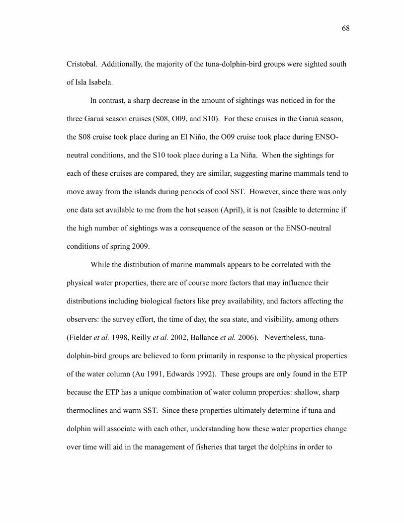
68
68
Cristobal. Additionally, the majority of the tuna-dolphin-bird groups were sighted south
of Isla Isabela.
In contrast, a sharp decrease in the amount of sightings was noticed in for the
three Garuá season cruises (S08, O09, and S10). For these cruises in the Garuá season,
the S08 cruise took place during an El Niño, the O09 cruise took place during ENSO-
neutral conditions, and the S10 took place during a La Niña. When the sightings for
each of these cruises are compared, they are similar, suggesting marine mammals tend to
move away from the islands during periods of cool SST. However, since there was only
one data set available to me from the hot season (April), it is not feasible to determine if
the high number of sightings was a consequence of the season or the ENSO-neutral
conditions of spring 2009.
While the distribution of marine mammals appears to be correlated with the
physical water properties, there are of course more factors that may influence their
distributions including biological factors like prey availability, and factors affecting the
observers: the survey effort, the time of day, the sea state, and visibility, among others
(Fielder et al. 1998, Reilly et al. 2002, Ballance et al. 2006). Nevertheless, tuna-
dolphin-bird groups are believed to form primarily in response to the physical properties
of the water column (Au 1991, Edwards 1992). These groups are only found in the ETP
because the ETP has a unique combination of water column properties: shallow, sharp
thermoclines and warm SST. Since these properties ultimately determine if tuna and
dolphin will associate with each other, understanding how these water properties change
over time will aid in the management of fisheries that target the dolphins in order to

69
69
catch the tuna.
My thesis data sets show an increase in the observation of tuna-dolphin-bird
groups during periods when SST were warm and the thermoclines were shallow and
sharp (i.e. when prey is assumed to be abundant (A09). Additionally, the ENSO cycle
plays a significant role in controlling the depth of the thermocline, although the current
data are too limited for any conclusive evidence. It is expected that additional fieldwork
should show that there are greater numbers of tuna-dolphin-bird groups during ENSO-
neutral periods than during El Niño (deep thermoclines) or La Niña (cool SST) events.
Additionally, yellowfin tuna may be limited both horizontally and vertically
within the GMR as large (+10°C) temperature fluctuations occur from year to year.
When these occur, tuna should change their distribution to follow the warmer water. If
the formation of tuna-dolphin-bird assemblages were determined solely on the depth of
their limitation, then most groups would form east of the GMR. However, very few
groups were observed here. Rather they were concentrated around southern Isla Isabela.
With only limited CTD data from this region, it is difficult to determine what the typical
depth of the thermocline in the area is. However, future work may show that south of
Isla Isabela the thermoclines are shallow (i.e. the EUC should be close to the surface).
This, along with the high prey abundance indicated by high chlorophyll concentrations,
may indicate this area should have optimal conditions for the formation of these
multispecies groups.

70
70
Future Work
Additional Surveys
It is difficult to ascribe any statistical significance in the trends observed in this
study due to the limited amount of data. Additional surveys are required during each
combination of the months observed in the GMR (April, June, and September/October)
and the different possible ENSO conditions. These surveys should include not only the
present stations occupied in the oceanographic surveys along the outer limits of the
GMR, but also within the archipelago such as CTDs of opportunity done in the J10
survey. If these surveys continue to support the observations made in this study, the
analytical trends noted in this these could be statistically supported.
Applications
The data from this survey could be used to reduce the amount of dolphin bycatch
in small artisanal fisheries by arranging the gillnet fishing season around periods when
the conditions are unfavorable for the formation of these assemblages. The other fishing
methods permitted in the GMR would not need to be subject to the same closures
because they have a low potential for dolphin bycatch. For example, within the GMR,
the artisanal gillnet tuna fishing season could be limited to periods when the SST are
cooler than average such as during the Garuá season and La Niña events. This would
require a dynamic method of managing the fishery, rather than a static method of
arbitrary area closings, etc that is generally used. This method of fishery management
has been shown to be successful in other areas that experience strong annual and

71
71
interannual changes (Bakun et al. 2010). In this way, the bycatch of marine mammals in
artisanal tuna fisheries may be more effectively managed, and eventually reduced.

72
72
LITERATURE CITED
Alva, J. J. 2009. Carbon productivity and flux in the marine ecosystems of the
Galapagos Marine Reserve based on cetacean abundances and trophic indices.
Revista de Biología Marina y Oceanografía 44: 109-122.
Au, D. W. 1991. Polyspecific nature of tuna schools: shark, dolphin, and seabird
associates Fishery Bulletin. 89: 343-354.
Au, D. W. and R. L. Pitman. 1988. Seabird relationships with tropical tunas and
dolphins. Pages 174-212 in J. Burger ed. Seabirds and Other Marine Vertebrates:
Competition, Predation, and Other Interactions. Columbia University Press, New
York.
Au, D. W. K. and W. L. Perryman. 1985. Dolphin habitats in the Eastern Tropical
Pacific. Fishery Bulletin 83: 623-643.
Bakun, A., E. Babcock, S. Lluch-Cota, C. Santora and C. Salvadeo. 2010. Issues of
ecosystem-based management of forage fisheries in “open” non-stationary
ecosystems: the example of the sardine fishery in the Gulf of California. Reviews
in Fish Biology and Fisheries 20: 9-29.
Ballance, L. T., R. L. Pitman and P. C. Fiedler. 2006. Oceanographic influences on
seabirds and cetaceans of the eastern tropical Pacific: a review. Progress In
Oceanography 69: 360-390.
Ballance, L. T., R. L. Pitman and S. B. Reilly. 1997. Seabird community structure along
a productivity gradient: importance of competition and energetic constraint.
Ecology 78: 1502-1518.
Block, B. A., J. E. Keen, B. Castillo, H. Dewar, E. V. Freund, D. J. Marcinek, R. W. Brill
and C. Farwell. 1997. Environmental preferences of yellowfin tuna (Thunnus
albacares) at the northern extent of its range. Marine Biology 130: 119-132.
Brill, R. and M. Lutcavage. 2001. Understanding environmental influences on
movements and depth distributions of tunas and billfishes can significantly
improve population assessments. Fishery Bulletin 100: 179-198.
Brill, R. W., B. A. Block, C. H. Boggs, K. A. Bigelow, E. V. Freund and D. J. Marcinek.
1999. Horizontal movements and depth distribution of large adult yellowfin tuna
(Thunnus albacares) near the Hawaiian Islands, recorded using ultrasonic
telemetry: implications for the physiological ecology of pelagic fishes. Marine
Biology 133: 395-408.

73
73
Broadhead, G. C. and I. Barrett. 1964. Some factors affecting the distribution and
apparent abundance of yellowfin and skipjack tuna in the Eastern Pacific Ocean.
Inter-American Tropical Tuna Commission Bulletin 8: 419 - 473.
Cane, M. 1983. Oceanographic events during El Niño. Science 222: 1189-1195.
Castro, C. and P. Rosero. 2010. Interaccion de cetaceos menoeres con artes de pesca
artesanal en el Parque Nacional Machalilla - Ecuador. Esfuerzos para Mitigar el
Impacto de Actividades Pesqueras en Cetaceos en los Paises de Pacifico Sudeste
1: 19-26.
Collette, B. B. and C. E. Nauen. 1983. FAO Species Catalogue. Vol. 2. Scombrids of the
world. An annotated and illustrated catalogue of Tunas, Makerels, Bonitos, and
related species known to date. FAO Fishery Symposium 125: 1-137.
Conroy, J. L., A. Restrepo, J. T. Overpeck, M. Steinitz-Kannan, J. E. Cole, M. B. Bush
and P. A. Colinvaux. 2009. Unprecedented recent warming of surface
temperatures in the eastern tropical Pacific Ocean. Nature Geoscience 2: 46-50.
CPS/NWS. 2011. Monitoring and Data. Climate Predition Center National Weather
Service Internet Team, NOAA/ National Weather Service National Centers for
Environmental Prediction.
CTPJMP. 2009. Capítulo Pesca del Plan de Manejo de la Reserva Marina de Galápagos
Pages 47. Comisión Técnica Pesquera de la Junta de Manejo Participativo,
Galapagos, Ecuador.
Donguy, J. and G. Meyers. 1987. Observed and modelled topography of the 20 C
isotherm in the tropical Pacific. Oceanologica acta 10: 41-48.
Ecuador Ministry of the Environment. 2008. Reglamento Especial para la actividad
pesquera en la Reserva Marina de Galápagos. La Ministra del Ambiente. Quito,
Ecuador.
Edwards, E. F. 1992. Energetics of associated tunas and dolphins in the eastern tropical
Pacific Ocean: A basis for the bond. Fishery Bulletin 90: 678-690.
Ely, B., J. Vinas, J. Alvarado Bremer, D. Black, L. Lucas, K. Covello, A. Labrie and E.
Thelen. 2005. Consequences of the historical demography on the global
population structure of two highly migratory cosmopolitan marine fishes: the
yellowfin tuna (Thunnus albacares) and the skipjack tuna (Katsuwonus pelamis).
BMC Evolutionary Biology 5: 1-19.
Espinosa-Carreon, T. L., P. T. Strub, E. Beier, F. Ocampo-Torres and G. Gaxiola-Castro.

74
74
2004. Seasonal and interannual variability of satellite-derived chlorophyll
pigment, surface height, and temperature off Baja California. Journal of
Geophysical Research 109: C03039.
Ferguson, M. C., J. Barlow, P. Fiedler, S. B. Reilly and T. Gerrodette. 2006. Spatial
models of delphinid (family Delphinidae) encounter rate and group size in the
eastern tropical Pacific Ocean. Ecological Modelling 193: 645-662.
Fiedler, P. 2010. Comparison of objective descriptions of the thermocline. Limnology
and Oceanography Methods 8: 313-325.
Fielder, P. C. 2002. Environmental change in the Eastern Tropical Pacific Ocean: a
review of ENSO and decadal variability. NOAA Administrative Report LJ-02-16
1-38.
Fielder, P. C., J. Barlow and T. Gerrodette. 1998. Dolphin prey abundance determined
from acoustic backscatter data in eastern Pacific surveys. Fishery Bulletin 96:
237-247.
Gargett, A. E. 1991. Physical processes and the maintenance of nutrient-rich euphotic
zones. Limnology and Oceanography 36: 1527-1545.
Gooding, R. M., W. H. Neill and A. E. Dizon. 1981. Respiration rates and low-oxygen
tolerance in skipjack tuna, Katsuwonus pelamis. Fishery Bulletin 79: 31-48.
Green, R. E. 1967. Relationship of the thermocline to sucess of purse seining for tuna.
Transactions of the American Fisheries Society 96: 126-130.
Hasegawa, D., M. R. Lewis and A. Gangopadhyay. 2009. How islands cause
phytoplankton to bloom in their wakes. Geophysical Research Letters 36:
L20605.
Hasegawa, D., H. Yamazaki, R. G. Lueck and L. Seuront. 2004. How islands stir and
fertilize the upper ocean. Geophysical Research Letters 31: L16303.
Jennings, S., A. S. Brierley and J. W. Walker. 1994. The inshore fish assemblages of the
Galápagos archipelago. Biological Conservation 70: 49-57.
Kessler, W. S. 1990. Observations of long Rossby waves in the Northern Tropical
Pacific. Journal of Geophysical Research 95: 5183-5217.
Kessler, W. S., M. J. Mcphaden and K. M. Weickmann. 1995. Forcing of intraseasonal
Kelvin waves in the equatorial Pacific. Journal of Geophysical Research 100:
10613-10631.

75
75
Mangel, J. C., J. Alfaro-Shigueto, K. Van Waerebeek, C. Caceres, S. Bearhop, M. J. Witt
and B. J. Godley. 2010. Small cetacean captures in Peruvian artisanal fisheries:
high despite protective legislation. Biological Conservation 143: 136-143.
Mills, K. L. 1998. Multispecies seabird feeding flocks in the Galápagos Islands. The
Condor 100: 277-285.
Morrison, J. M., S. Banks, D. Kamykowski, L. Xie, G. Feldman, B. A. Schaeffer, W. V.
Sweet, A. Mcculloch and Y. Liu. 2009. Connectivity and upwelling dynamics in
the Galapagos Marine Reserve (GMR). Pages 122-126 in M. Wolff and M.
Gardener eds. Galapagos Science Symposium. The Charles Darwin Foundation,
Puerto Ayora, Santa Cruz, Galapagos Islands.
Oxenford, H. 2002. Review of Eastern Tropical Pacific (ETP) Ocean ecosystem studies.
CIE Ecosystem Review Meeting 1: 1- 23.
Palacios, D. M. 2004. Seasonal patterns of sea-surface temperature and ocean color
around the Galápagos: regional and local influences. Deep Sea Research Part II:
Topical Studies in Oceanography 51: 43-57.
Palacios, D. M., S. J. Bograd, D. G. Foley and F. B. Schwing. 2006. Oceanographic
characteristics of biological hot spots in the North Pacific: a remote sensing
perspective. Deep Sea Research Part II: Topical Studies in Oceanography 53:
250-269.
Palacios, D. M., S. J. Bograd, R. Mendelssohn and F. B. Schwing. 2004. Long-term and
seasonal trends in stratification in the California Current, 1950 - 1993. Journal of
Geophysical Research 109: C10016.
Perrin, W. F., R. R. Warner, C. H. Fiscus and D. B. Holtz. 1973. Stomach contents of
porpoise Stenella spp. and yellowfin tuna Thunnus albacares in mixed species
aggregations. Fishery Bulletin 71: 1077-1092.
Polacheck, T. 1987. Relative abundance, distribution, and inter-specific relationshops of
cetacean schools in the Eastern Tropical Pacific. Marine Mammal Science 3: 54-
77.
Redfern, J. V., J. Barlow, L. T. Ballance, T. Gerrodette and E. A. Becker. 2008. Absence
of scale dependence in dolphin–habitat models for the eastern tropical Pacific
Ocean. Marine Ecology Progress Series 363: 1-14.
Reilly, S. B. 1990. Seasonal changes in distribution and habitat differences among
dolphins in the eastern tropical Pacific. Marine Ecology Progress Series 66: 1-11.

76
76
Reilly, S. B., P. C. Fiedler, T. Gerrodette, L. T. Ballance, R. L. Pitman, J. M. Borberg and
R. C. Holland. 2002. Eastern Tropical Pacific dolphin habitats - interannual
variability 1986-2000. NOAA Administrative Report LJ-02-21.
Ribic, C. A. and D. G. Ainley. 1997. The relationships of seabird assemblages to
physical habitat features in Pacific equatorial waters during spring 1984–1991.
ICES Journal of Marine Science: Journal du Conseil 54: 593-599.
Riedman, M. 1990. The pinnipeds: seals, sea lions, and walruses. University of
California Press, Berkley.
Saltzman, J. and K. F. Wishner. 1997. Zooplankton ecology in the eastern tropical
Pacific oxygen minimum zone above a seamount: 1. general trends. Deep Sea
Research Part I: Oceanographic Research Papers 44: 907-930.
Schaefer, K., D. Fuller and B. Block. 2009. Vertical movements and habitat utilization of
skipjack (Katsuwonus pelamis), yellowfin (Thunnus albacares), and bigeye
(Thunnus obesus) tunas in the Equatorial Eastern Pacific Ocean, ascertained
through archival tag data. Tagging and Tracking of Marine Animals with
Electronic Devices 9: 121-144.
Scott, M. D. and S. J. Chivers. 2009. Movements and diving behavior of pelagic spotted
dolphins. Marine Mammal Science 25: 137-160.
Scott, M. D. and K. L. Cattanach. 1998. Diel patterns in aggregations of pelagic dolphins
and tunas in the Eastern Pacific. Marine Mammal Science 14: 401-422.
Silva, M. A., R. Feio, R. Prieto, J. M. Gonçalves and R. S. Santos. 2002. Interactions
between cetaceans and the tuna fishery in the Azores. Marine Mammal Science
18: 893-901.
Spear, L. B., L. T. Ballance and D. G. Ainley. 2001. Response of seabirds to thermal
boundaries in the tropical Pacific: the thermocline versus the Equatorial Front.
Marine Ecology Progress Series 219: 275-289.
Steger, J., C. Collins and P. Chu. 1998. Circulation in the Archipiélago de Colón
(Galapagos Islands), November, 1993. Deep-Sea Research Part II 45: 1093-1114.
Sweet, W. V., J. M. Morrison, D. Kamykowski, B. A. Schaeffer, S. Banks and A.
Mcculloch. 2007. Water mass seasonal variability in the Galápagos Archipelago.
Deep Sea Research Part I: Oceanographic Research Papers 54: 2023-2035.
Wade, P. R. and T. Gerrodette. 1993. Estimates of cetacean abundance and distribution in

77
77
the Eastern Tropical Pacific Report of the International Whaling Commission 43:
477-494.
Wyrtki, K. 1966. Oceanography of the Eastern Equatorial Pacific Ocean. Oceanography
and Marine Biology Annual Review 4: 33-68.
Wyrtki, K. 1964. The thermal structure of the Eastern Tropical Pacific Ocean.
Ergaenzungsheft Reihe A (8°), Nr.6 zur Deutschen Hydrographicschen
Zeitschrift A 8°: 6-84.
Yen, P. P. W., W. J. Sydeman and K. D. Hyrenbach. 2004. Marine bird and cetacean
associations with bathymetric habitats and shallow-water topographies:
implications for trophic transfer and conservation. Journal of Marine Systems 50:
79-99.

78
78
APPENDIX
SST FIGURES
Figure A-1. Sea surface temperatures of the area between the Ecuador mainland and the Galapagos
Islands, showing the location of the Equatorial Front in September 2008. Map based on values on
September 15, 2008, the approximate mid-point of the survey.
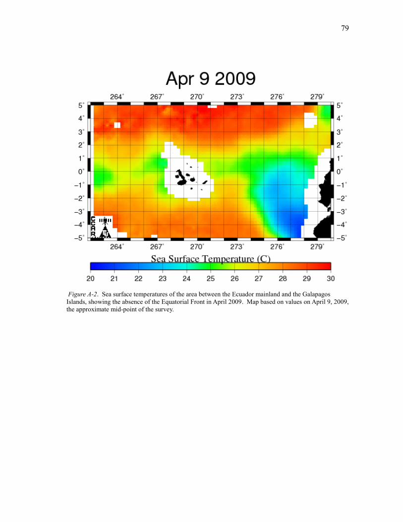
79
79
Figure A-2. Sea surface temperatures of the area between the Ecuador mainland and the Galapagos
Islands, showing the absence of the Equatorial Front in April 2009. Map based on values on April 9, 2009,
the approximate mid-point of the survey.

80
80
Figure A-3. Sea surface temperatures of the area between the Ecuador mainland and the Galapagos
Islands, showing the location of the Equatorial Front in October 2009. Map based on values on October
17, 2009, the approximate mid-point of the survey.
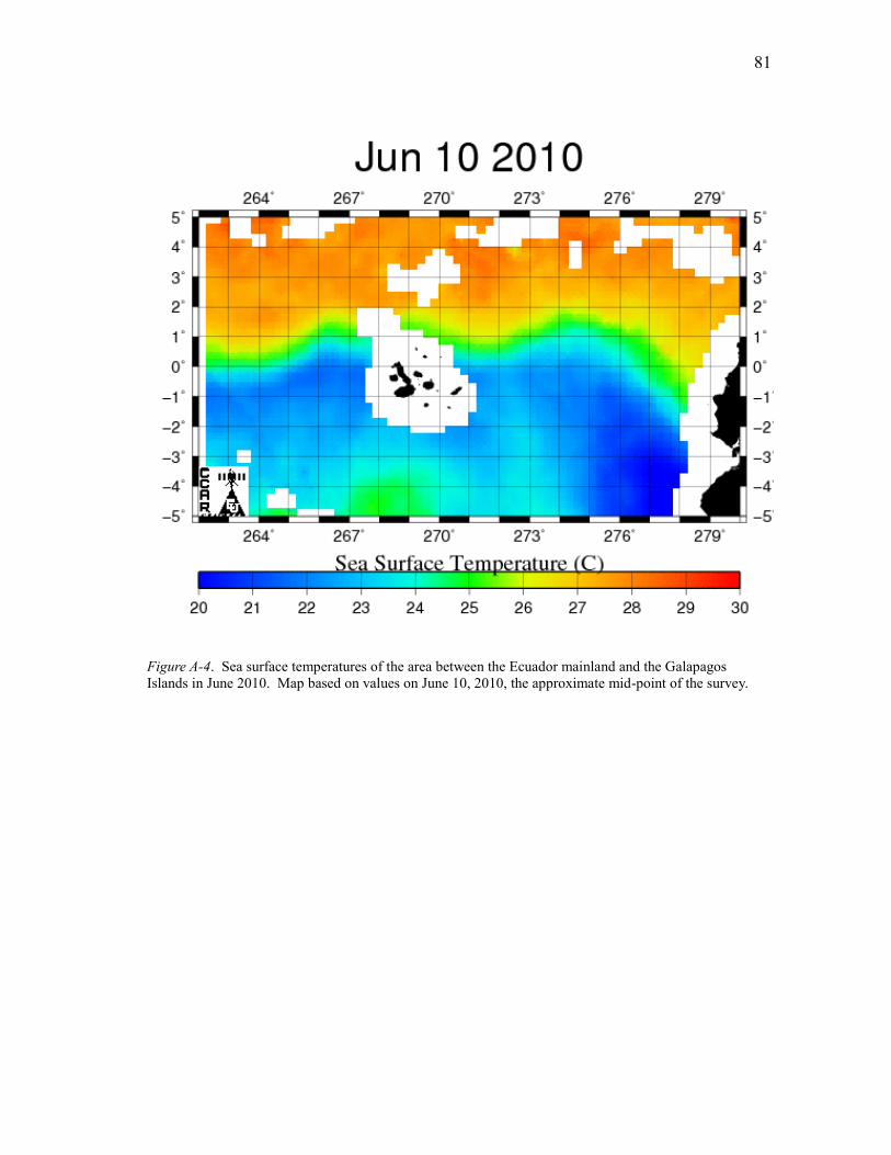
81
81
Figure A-4. Sea surface temperatures of the area between the Ecuador mainland and the Galapagos
Islands in June 2010. Map based on values on June 10, 2010, the approximate mid-point of the survey.

82
82
Figure A-5. Sea surface temperatures of the area between the Ecuador mainland and the Galapagos
Islands, showing the location of the Equatorial Front in September 2010. Map based on values on
September 30, 2010, the approximate mid-point of the survey.

83
83
VITA
Name: Michelle Lynn Johnston
Address: c/o Dr. Doug Biggs, MS 3146, Texas A&M University, College
Station, TX 77840
Email Address: [email protected]
Education: B.S., Biology with All-College Honors, Westminster College, 2009
M.S., Oceanography, Texas A&M University, 2011
Recommended