DI
SC
US
SI
ON
P
AP
ER
S
ER
IE
S
Forschungsinstitut zur Zukunft der ArbeitInstitute for the Study of Labor
Job Satisfaction and Self-Selection into the Public or Private Sector: Evidence from a Natural Experiment
IZA DP No. 7644
September 2013
Natalia Danzer
Job Satisfaction and Self-Selection
into the Public or Private Sector: Evidence from a Natural Experiment
Natalia Danzer Ifo Institute, University of Munich (LMU)
and IZA
Discussion Paper No. 7644 September 2013
IZA
P.O. Box 7240 53072 Bonn
Germany
Phone: +49-228-3894-0 Fax: +49-228-3894-180
E-mail: [email protected]
Any opinions expressed here are those of the author(s) and not those of IZA. Research published in this series may include views on policy, but the institute itself takes no institutional policy positions. The IZA research network is committed to the IZA Guiding Principles of Research Integrity. The Institute for the Study of Labor (IZA) in Bonn is a local and virtual international research center and a place of communication between science, politics and business. IZA is an independent nonprofit organization supported by Deutsche Post Foundation. The center is associated with the University of Bonn and offers a stimulating research environment through its international network, workshops and conferences, data service, project support, research visits and doctoral program. IZA engages in (i) original and internationally competitive research in all fields of labor economics, (ii) development of policy concepts, and (iii) dissemination of research results and concepts to the interested public. IZA Discussion Papers often represent preliminary work and are circulated to encourage discussion. Citation of such a paper should account for its provisional character. A revised version may be available directly from the author.
IZA Discussion Paper No. 7644 September 2013
ABSTRACT
Job Satisfaction and Self-Selection into the Public or Private Sector: Evidence from a Natural Experiment*
Are public sector jobs better than private sector jobs? To answer this question, this paper investigates observed differences in job satisfaction between public- and private-sector workers and disentangles the effect of worker sorting from the one caused by sector-specific job characteristics. A natural experiment – the massive privatization process in post-Soviet countries – allows correcting potential self-selection bias. Industry-specific privatization probabilities are assigned to workers based on unique individual-level survey information regarding pre-determined Soviet jobs during the 1980s. The results reveal a causal public-sector satisfaction premium and a negative selection of individuals into the public sector. Part of the public-private satisfaction gap can be explained by the different availability of fringe benefits in the two sectors. JEL Classification: J28, J45, J31, J32 Keywords: public sector, job satisfaction, self-selection, quasi-experiment, privatization,
fringe benefits Corresponding author: Natalia Danzer ifo Institute ifo Center for Labour Market Research and Family Economics Poschingerstr. 5 81679 Munich Germany E-mail: [email protected]
* I am very grateful to Andrew Clark, Victor Lavy and Jonathan Wadsworth for valuable comments and discussions. I also benefited from inspiring feedback from J. David Brown, Alexander M. Danzer, Peter Dolton, Francesco Fasani, Colin Green, Helmut Rainer, Andrew Oswald, Chiara Rosazza-Bondibene, Analía Schlosser, Anna Vignoles, and participants at the Annual Conferences of the Scottish Economic Society and the Royal Economic Society as well as from seminar participants at the Royal Holloway College and Milan University. Sincere thanks to IZA, the ULMS consortium and the DIW Berlin for making the dataset available and to Natalia Kharchenko and Volodymyr Paniotto at KIIS for helpful information on the survey and the dataset. Thank you to Norberto Pignatti and Lena Ruckh for kindly sharing their retrospective ULMS data files with me and to Alexander Danzer for providing me with the relevant data extract from the UHBS needed for calculating the second instrument.
1
1 Introduction
Do public sector worker receive rents? This paper revisits the research on public-
private wage differentials from a subjective well-being perspective by analyzing differences
in job satisfaction between state and private sector employees. While several recent studies
found public-sector workers to be on average more satisfied with their jobs than private-sector
workers this paper investigates the reason for this difference.1 In particular, it empirically
investigates whether public-private satisfaction gaps represent rents—that is, genuine
differences in objective job and workplace characteristics—or whether they are artificially
created by non-random self-selection of workers based on unobservable personality traits.
Economists have long been interested in public-sector labor markets due to the public
sector’s sheer size and its distinct characteristics and objectives that guide decision making
(e.g., collective wage setting, affirmative action) (Blank 1985; Ehrenberg and Schwarz 1987;
Gregory and Borland 1999). In times of high budget deficits, it is also debated whether
public-sector workers are over-compensated. This debate has not only fiscal implications (as
public-sector wages must be borne by taxpayers), but affects also the private sector in terms
of hiring and labor costs. The extensive theoretical literature—dating back to Adam Smith—
provides several explanations for wage differentials between industries or sectors and why it
might be optimal for certain firms to pay higher wages than others. One the one hand, wage
differences could reflect compensating differentials (monetary compensation for unpleasant
job aspects), implying market-clearing wages (Rosen 1987). On the other hand, these
differences could represent “rents” which may be driven by efficiency wages, rent-sharing
motives, union bargaining power, or political economy considerations (Katz and Autor 1999).
The classic empirical examination of sector wage differentials faces two major
challenges which the present study meets in the following way: first, the concept and
measurement of utility and disutility of labor. This would require a comprehensive measure
for total compensation (including non-wage pecuniary components and fringe benefits) as
well as a sound assessment of all job disamenities—both of which are extremely difficult to
1 Economic studies with an explicit focus on public-private sector job satisfaction differentials are: Clark and
Senik (2006) for France and the United Kingdom; Demoussis and Giannakopoulos (2007) for Greece; Ghinetti
(2007) for Italy; Heywood, Siebert, and Wei (2002) for the United Kingdom; Luechinger, Meier, and Stutzer
(2008) for 25 European and 17 Latin-American countries (analysis of life satisfaction); Luechinger, Stutzer, and
Winkelmann (2006) for 20 European countries and (2010) for Germany.
2
obtain.2 In the following empirical analysis, this challenge is addressed by focusing on job
satisfaction. The virtue of job satisfaction as a single measure is that it represents a
comprehensive assessment of all relevant job aspects, both amenities and disamenities, and
thus overcomes the problem of assessing pecuniary and non-pecuniary job aspects
(Hamermesh 2001). Hence, to the extent that differences in job satisfaction reflect an unequal
distribution of relative net advantages across sectors, the following analysis can detect sector-
specific rents and thus extend previous studies focusing on objective earnings measures.
The second challenge relates to unobserved heterogeneity among workers and the
need to account for possible self-selection into sectors. If certain sectors attract workers with
higher productivity or unobservable ability, simple least squares estimates of the wage
premium in this sector will be upward biased (Gibbons and Katz 1992). Correcting the
potential endogeneity of sector affiliation is crucial for identifying true sector differences and
yet non-trivial. In an ideal experimental setting, the problem of self-selection could be ruled
out by randomly assigning individuals to either the public or the private sector. Since such a
randomized experiment is unfeasible, the identification strategy of this study uses a unique
natural experiment that generated exogenous variation in the share of public-sector
employment. The tremendous changes in enterprise ownership structure in Eastern Europe’s
transition countries—from a situation of exclusive state ownership of all firms to a mixture of
privately and publicly owned firms—de facto randomly reallocated workers conditional on
their observables from the public to the private sector. The data come from a unique and
nationally representative survey of post-Soviet Ukraine (2003–2007) that contains almost
complete retrospective individual work histories since Soviet times.
This paper makes four contributions to the literature. First, in contrast to earlier studies
on public-private sector satisfaction differentials, this paper exploits a natural experiment to
correct for worker self-selection. Identification of the pure sector satisfaction differential is
based on exogenous variation in the ownership structure of firms stemming from the large-
scale privatization program accompanying the transition from a centrally planned to a market
economy. Second, the paper adds to the empirical evidence on inter-sector wage differentials
by providing indirect evidence of non-equalizing differences in total compensation as
measured by significant public-private job satisfaction gaps. Third, detailed survey
information on fringe benefits and payment schemes allows an assessment of whether the
2 Hamermesh (1999) provides an early account of the role of non-pecuniary aspects in the development of
overall earnings inequality in the United States. The most comprehensive attempt to measure total compensation
in the public and private sectors is by Danzer and Dolton (2011), who combine various data sources to account
for differences in, e.g., pension schemes, fringe benefits, and unemployment risks, in the United Kingdom.

3
public-sector satisfaction premium is driven by additional benefits. This analysis contributes
to the literature on the importance of job amenities and payment schemes for job and life
satisfaction (e.g., Helliwell and Huang 2010). Fourth, the paper analyzes job satisfaction in a
dynamically emerging economy based on a nationally representative dataset.
The results indicate that there indeed exists a causal positive and significant public
sector satisfaction premium. This implies that Ukrainian workers enjoy rents by working for a
public sector firm or organization. Part of these genuine differences between public and
private sector jobs can be attributed to pecuniary and non-pecuniary fringe benefits which are
more prevalent in the public than in the private sector. However, after correcting for self-
selection and controlling for differences in various job (dis)amenities and fringe benefits,
there remains a significant public-private job satisfaction gap.
The remainder of the paper is organized as follows. The next section discusses the
empirical problem of estimating the public-private job satisfaction differential faced in the
previous literature and describes the identification strategy of this paper as well as relevant
institutional background. Section 3 contains provides information on the dataset and on the
construction of the instrumental variables. The main regression results as well as several
robustness checks are presented in Section 4. The role of sector differences in the provision of
pecuniary and non-pecuniary benefits is assessed in Section 5. Section 6 concludes.
2 Identification Strategy and Institutional Background
In market-based economies, the observed allocation of workers in the labor market is
the outcome of a selection and sorting process through which individuals (and firms) search
and find their best matching jobs (and employees) according to their characteristics,
preferences, and information sets. Several empirical studies show that employees report
higher levels of job satisfaction the better the job matches their skills (Belfield and Harris
2002; Vieira 2005) implying utility gains from sorting in the labor market (Luechinger,
Stutzer, and Winkelmann 2006). However, a priori, there are no reasons why this sorting
process should lead to systematic higher job satisfaction levels in the state than in the private
sector (in a well-functioning labor market). And yet, the majority of the empirical studies on
the satisfaction differential between public- and private-sector workers find a public-sector
satisfaction premium (e.g., in Germany, Greece, Italy, and the United Kingdom).
One potential explanation for the observed job satisfaction gap are comparatively good
remuneration packages (including non-pecuniary job amenities) and working conditions in the

4
public sector. Sector differences in job and income security may also play a role, especially
during economic recessions (Luechinger, Meier, and Stutzer 2010). Public sector jobs could
also act as partial insurance of households against income risks in developing countries
(Rodrik 2000).3 Thus, if public-sector jobs were “truly better” and there were queues for them
(Krueger 1988), then, on average, satisfaction levels should be lower among private-sector
employees. In this case, the public-sector satisfaction premium would reflect “rents” (Clark
and Senik 2006; Luechinger, Meier, and Stutzer 2008; Luechinger, Stutzer, and Winkelmann
2010). A random reallocation of workers would not erase the observed satisfaction gap (i.e.,
the positive public-private satisfaction gap would remain after correcting for self-selection).
An alternative explanation posits that worker characteristics that drive the sorting
process are correlated with unobserved intrinsic levels of happiness. Even if both sectors
were similarly attractive, the sorting would imply a nonrandom allocation of workers in terms
of their inherent satisfaction levels. In this scenario, the positive public-private satisfaction
gap would only be spuriously caused by the fact that individuals from the upper part of an
underlying satisfaction distribution sort into the public sector (Heywood, Siebert, and Wei
2002). Ignoring such a self-selection of workers in the empirical estimation would yield
biased estimates of the true public satisfaction premium, while correcting for this type of
selection should eliminate the spurious satisfaction premium.
To date, empirical attempts to account for the problem of self-selection rely either on
panel methods (controlling for individual fixed effects: Clark and Senik 2006; Heywood,
Siebert, and Wei 2002), or on estimating endogenous switching regression models
(Luechinger, Stutzer, and Winkelmann 2006, 2010). Nevertheless, panel estimates could still
be biased since sector switching decisions are endogenously determined.4
Furthermore,
particularly low levels of job satisfaction prior to a voluntary leave (Boswell, Boudreau, and
Tichy, 2005) lead to overstating the true gain in satisfaction (similar to the Ashenfelter dip;
Ashenfelter (1978)).5 Consequently, standard panel data techniques are limited in their ability
to evaluate causal effects in the presence of self-selection. As regards switching regression
models, their identification rests on particular—and partly very restrictive—functional form
assumptions and ultimately requires valid instruments to act as exclusion restrictions in the
3 Another—unwanted and unintended—reason might be bribes (Luechinger, Meier, and Stutzer 2008).
4 Luechinger, Stutzer, and Winkelmann (2006) stress this point. This problem of fixed effects panel estimations
is also addressed in the literature on wage differentials (e.g., Gibbons and Katz 1992). 5 However, Clark, Diener, Georgellis, and Lucas (2008) show substantial anticipatory and adaptation effects of
life events on life satisfaction (e.g., unemployment). If the same was true for job satisfaction and voluntary job
changes, fixed effects models focusing on job switchers would underestimate the true satisfaction differential.
5
selection equation. Luechinger, Stutzer, and Winkelmann (2006, 2010) employ as instruments
the citizen status and parental occupation during childhood, respectively (in particular,
whether the father was a civil servant, whether he was a white collar worker and whether the
mother was working). However, as one cannot rule out that these instruments have a direct
effect on job satisfaction (beyond affecting sector choice) their validity might be jeopardized.6
2.1 Identification Strategy and Identifying Assumptions
In contrast to previous work, the identification strategy in this paper takes advantage
of a quasi-experiment created by the dramatic changes in the ownership structure of firms in
Ukraine that occurred after the collapse of the Soviet Union.7 Within about 10 years, the share
of private sector jobs in Ukraine grew from virtually zero to over 50 percent – due to large-
scale privatization of Soviet firms as well as the creation of new private firms (Figure 1). As a
result, part of the exclusively state-sector Soviet work force was de-facto exogenously
“reassigned” from the state to the private sector. However, even after the massive
privatization and restructuring processes of the 1990s state-sector ownership in 2003 was still
much more common in many industries than in advanced market economies. Owing to the
availability in the data of Soviet era information on the allocation of workers into what would
become state- or private-sector jobs in the data, the labor market sorting that took place after
the collapse of the Soviet Union can be measured and corrected for.
<< FIGURE 1 >>
The empirical analysis thus can answer the question: “Do public sector worker receive
rents or is the public job satisfaction premium simply driven by self-selection of workers?”
The methodology relies on instrumental variable techniques to identify the causal effect of
potential differences in workplace characteristics on job satisfaction. The constructed
instrumental variable comprises an exogenous probability of working in the private sector in
post-Soviet Ukraine based on pre-transition job characteristics (industry sector and
geographical location). The instrumental variable represents an intention to treat (in the first
stage), since not all individuals who were assigned to the treatment were actually treated.
Some individuals in the treatment group might have forgone “treatment” because their firm
6 Citizen status is strongly correlated with cultural background which in turn might affect job satisfaction.
Father’s occupational choice might be determined by unobserved characteristics which are intergenerationally
transmitted and thus also simultaneously affect their offspring’s sector choice and satisfaction levels. 7 Focusing on another research question, Fuchs-Schündeln and Schündeln (2005) use a similar identifying
assumption to exploit the German reunification “experiment” to purge the estimation of precautionary savings
from possible self-selection bias into low-risk occupations. In their setup, reunification is interpreted as a “re-
assignment” of income risks for certain occupational groups.
6
was never privatized or because they switched industries during the 1990s.8 The estimated
effect must be interpreted as local average treatment effect (LATE) since identification stems
from individuals who comply with their assigned treatment and switch sectors accordingly
(Imbens and Angrist 1994).
For the identification strategy to be valid, the instrumental variables need to satisfy the
exclusion restriction. Since the treatment variable is assigned according to Soviet industry
(and region) affiliation, the exclusion requires that during Soviet times workers were
randomly allocated across “would-be private” and “would-be public” industries (and regions)
with respect to their intrinsic satisfaction levels. There are several reasons and particular
features of the Soviet labor market why this identifying assumption is likely to hold (even
more so when one considers a random allocation conditional on predetermined observable
personal characteristics). First, from the perspective of a Soviet employee in the 1980s, the
collapse of the Soviet Union with its economic and political implications was unexpected and
unforeseeable.9 Hence, one can rule out anticipatory sorting behavior. Second, in the Soviet
Union there was no private sector or any sector with features similar to those of the private
sector of advanced market economies (e.g., profit-maximizing firms, competition, hard budget
constraints, job uncertainty) and, hence, workers could not self-select themselves into firms or
industry because of them being privately or publicly owned or showing features of typical
“Western” private or public firms. Third, job security as well as the provision of fringe
benefits did not differ across industries. Full employment was guaranteed by the constitution
and implemented by the state. Wages, working hours, and working conditions were set
centrally by the government, and the wage distribution was relatively compressed (see Brown
1973; Gregory and Collier 1988). Furthermore, social security, free medical services, social
benefits, and fringe benefits were provided irrespective of economic or industrial sector
(Flemming and Micklewright 2000; Friebel and Guriev 2005). Fourth, individual freedom to
choose the field of study, one’s employer or even one’s region of living was extremely limited
or not existent. Since the Soviet Union was run and organized along political motives and
principles, individual educational paths and fields of specialization, as well as professional
advancement, were more closely connected to political loyalty and political decisions rather
than to individual ability or preferences (Titma and Roots 2006). According to estimates,
about 60 to 70 percent of graduates were allocated to their first job by the government to meet
labor requirements in certain industries and regions (Haddad 1972). In addition, individuals’
8 In the sample, 55 percent of the workers work in the same industry they used to work in during Soviet times.
9 Estrin, Hanousek, Kocenda, and Svejnar (2009) provide a recent review on the effects of privatization.
7
labor market choices and mobility were limited due to the internal passport system as well as
the administrative allocation of housing in the Soviet Union (Gregory and Kohlhase 1988).
The spatial segregation of planned production limited the diversity of industries within certain
regions (Friebel and Guriev 2005). In extreme cases, the entire population of an area was
working in a single large state-owned enterprise (one-company towns). Against this
background and given the particular features of the Soviet labor market, it seems plausible
that the ex-ante privatization probability is unrelated to the intrinsic satisfaction levels of
workers. Hence, the distribution of workers across different industries (within geographical
regions) during the Soviet Union can be seen as a valid counterfactual against which the post-
Soviet allocation of workers across publicly and privately owned firms can be assessed.
Another important identifying assumption is that the instrument (the ex-ante
privatization probability) has no direct effect itself on today’s job satisfaction. This aspect is
critically discussed below in the section on robustness tests, which also contains a sensitivity
test with respect to those individuals who have personally experienced privatization in recent
years and should be thus supposedly more strongly negatively affected (Section 4.3).
However, when dropping these critical observations the results become even stronger. Finally,
the instruments need to satisfy the monotonicity assumption as it likely does, because it is
implausible that persons generally preferring to work in the private sector reverse their
preferred choice due to being assigned to the private sector by the instrument.
2.2 Evolution of the Private Sector in Post-Soviet Ukraine
During the transition from a planned to a market economy a private sector evolved as
the consequence of the privatization process, through which formerly state-owned entities
were transferred to private ownership, and the creation of completely new firms (de novo
firms), which had never been owned by the state. The privatization process in Ukraine started
in 1992 and progressed more slowly than in most other Central and Eastern European
countries (Brown, Earle, and Telegdy 2006). Between 1992 and 2004, more than 96,549
formerly state-owned entities were transferred to private ownership by means of privatization
(State Statistics Committee of Ukraine 2005). Privatization took place in all industrial sectors,
but the extent of privatization varied substantially across industries (see Section 3.2). The
political goal to privatize quickly and socially acceptable, led to large-scale mass
privatizations as predominant method (involving the distribution of free privatization
certificates to citizens or share transfers to employees), especially in the early 1990s
8
(Pivovarsky 2001). As Brown, Earle, and Telegdy (2006) point out, the privatization process
was universal, implying that firms were less selectively and carefully chosen than typically
done in Western countries. This fact further strengthens the validity of the identification
strategy. Another important aspect is that there were only very few jobs that were ended
mainly because of privatization and this is true for all industries (less than one percent).
Figure 2 provides an overview of the reasons why jobs that started during the Soviet period
were terminated during the transition process. The figure contains only answers related to the
restructuring process. In the late 1990s and early 2000s the majority of jobs ended due to
“personnel reductions,” “closing down of enterprise,” and “reorganization of enterprise”.
<< FIGURE 2 >>
After its official start in 1992, the privatization process only gained momentum after
the Ukrainian government launched a revised mass privatization program at the end of 1994,
which had been prepared with the support of Western donors and advisors (USAID, World
Bank, EU, and EBRD) (USAID 1999).10
The program’s goal was to privatize the universe of
Ukraine’s approximately 10,000 medium and large industrial enterprises by 1998 based on
the following objectives: (i) rapid and equitable distribution of shares to Ukrainian citizens,
(ii) development of capital markets and the respective infrastructure, and (iii) quick creation
of a critical mass of privately owned enterprises that would trigger relevant modernization
processes in the economy (USAID 1999).11
Generation of state revenues was not a primary
aim of the mass privatization program (Grygorenko and Lutz 2007). In addition to the mass
privatization of medium- and large-scale enterprises, about 40,000 shops and retail
establishments were privatized by means of employee buyouts or cash auctions. Owing to the
design of the mass privatization program the resulting ownership became widely dispersed
and dominated by insiders (managers and workers) (Grygorenko and Lutz 2007).
Apart from privatization, the destruction and creation of firms affected the share of
private employment across industry sectors and also caused a shrinking of some industries
(manufacturing) and growth of others (services). Some individuals may have been forced to 10
The Ukrainian Parliament approved the law on the First Privatization Program in July 1992 (Verkhovna Rada:
The State Privatization Program for 1992; see Grygorenko and Lutz 2007). 11
Mass privatization in Ukraine was carried out by distributing privatization certificates or vouchers to all
citizens. These vouchers could be used to purchase shares of enterprises. Preferential purchase rights were given
to employees and managers and remaining shares were sold to other persons holding privatization certificates
(USAID 1999). In the largest enterprises, about 25 percent of shares were sold to employees and the public, the
state initially kept between 25 to 51 percent of shares (especially in so-called strategic enterprises), and the
remaining shares were sold via cash and/or investment tenders or local stock exchange sales (USAID 1999). In
1995, the Ukrainian Parliament issued a list of 5,200 “enterprises banned from privatization in view of their
importance for the national economy.” These were mainly enterprises in the energy sector (power networks and
energy systems, hydro and nuclear power stations, combined heat and power stations) (USAID 2000).
9
leave their state-sector employment due to plant closure and seek new job opportunities
elsewhere. Since the creation of new firms and jobs almost exclusively occurred in the private
sector, these structural changes de facto also reallocated individuals into the private-sector.
3 Dataset, Variables, and Sample Description
The analysis is based on the Ukrainian Longitudinal Monitoring Survey (ULMS), a
nationally representative panel dataset of individuals aged 15 to 72 who were interviewed in
three waves in the years 2003, 2004, and 2007.12
The survey provides detailed information on
individual labor market activity, workplace and job characteristics, plus all relevant individual
and household socio-demographic characteristics.
Two special features make this dataset unique and especially suitable for addressing
the research question. First, the data provide detailed retrospective information about the
individuals’ labor market activities and job characteristics during the time of the Soviet Union
as well as individual labor market histories during the transition process, including
information on whether and, if so, when their workplaces were privatized.13
Specifically,
respondents were asked to provide labor market information for December 1986 and
December 1991, as well as a complete job history spanning the years 1997-2007. The years
1986 and 1991 were chosen because they are important years in Ukrainian history (Chernobyl
catastrophe in 1986; 1991 as the year before independence) and so serve as memory anchors
to reduce recall error (Ganguli and Terrell 2006).14
Altogether, there are 5,786 individuals in
the cross-section 2003 for whom this Soviet labor market information is available, meaning
that complete labor market information exists for almost all sampled individuals who were of
working age when the Soviet Union collapsed (official unemployment was absent in the
Soviet Union). The Soviet labor market information along with the privatization information
is used to construct one of the instrumental variables. Second, the survey collects detailed
ownership information about the respondents’ current workplaces (13 different categories)
and thus allows an exact classification of respondents into public or private employment.15
12
The survey was conducted by the Kiev Institute for Sociology (KIIS) following a multistage sampling
procedure. Details on the sampling procedure can be found in the technical reports provided by KIIS. 13
The reliability of self-reported ownership status in the ULMS is discussed by Brown, Earle, and Vakhitov
(2006), who use the ULMS to analyze wage and employment effects of privatization. They emphasize the
careful wording and the fact that workers were directly involved in any privatization process, which likely
increases the accuracy of the answers. However, a measurement error in this variable (state-sector employment)
should lead to a downward bias in the estimated coefficients. 14
Furthermore, as wages were highly regulated and determined by a centralized wage grid during Soviet times
the likelihood for correct recalls of Soviet wages should be high (Ganguli and Terrell 2006). 15
This is an advantage compared to some datasets used in the previous literature that lack direct information on
firm ownership (e.g., the European Social Survey used amongst other data sources in Luechinger et al. 2008).
10
Regarding the sample for the job satisfaction analysis, there are 3,583 individuals in
paid employment at the time of the interview in 2003 (see Table A 1 in the Online Appendix).
Out of these, 2,556 held a job during Soviet times. Missing values in several variables reduce
the number of observations to 1,491. The main estimation sample is based on observations
from all three survey waves and includes all individuals who have a paid job at the time of the
interview, yielding a pooled sample of 4,191 observations (unbalanced panel).16
The second, alternative instrumental variable is creating using the Ukrainian
Household Budget Survey (UHBS). The UHBS is an annual cross-section of around 9,000
households and about 25,000 individuals and is conducted by the State Statistics Committee
of Ukraine (UkrStat). Calculations of the instrumental variable are based on four survey years
(2003–2006) and make use of the individual level labor market information on industrial
sector, enterprise ownership, and place of residence.
3.1 Dependent and Explanatory Variables
The dependent variable, job satisfaction, is measured by the question “Tell me, please,
how satisfied are you with your current job?” to which respondents can answer on a five-
point Likert scale ranging from 1 (fully dissatisfied) to 5 (fully satisfied). This question can be
interpreted as a comprehensive judgment of all relevant job aspects. The main analysis will
employ this categorical dependent variable.17
<< FIGURE 3 >>
How satisfied are workers in the private and state sectors in post-Soviet Ukraine?
Figure 3 presents the raw unconditional job satisfaction levels in both sectors for the pooled
sample of workers.18
Almost twice as many workers in the private sector are entirely
dissatisfied with their job (12.3 vs. 6.5 percent, respectively). Focusing on the other end of the
spectrum, the share of fully satisfied workers in the public sector surpasses the one in the
private sector by 5 percentage points. These distributions imply that state-sector workers are
generally more satisfied with their jobs than are their private-sector counterparts. A similar
16
As a sensitivity check, the main regressions are re-estimated based on a larger sample by dropping the variable
measuring risk aversion, which was collected in 2007 only (this increases the pooled sample size to 5,142
observations; the 2003 sample increases from 1,491 to 2,059; see Table A 1, Online Appendix). 17
Two surveys asked about job satisfaction during Soviet times: the World Values Survey 1981 (conducted in
the Soviet region Tambov) and the Consolidation of Democracy in Central and Eastern Europe Survey of
January 1991 (Ukrainian Soviet Socialist Republic). As both lack relevant variables they cannot be used to
analyze the relationship between job characteristics and job satisfaction before the start of the transition process. 18
Figure 3 is based on the sample used in the regressions. The picture remains almost the same when using the
complete ULMS sample including young individuals (graph not shown, but available from author upon request).
11
pattern in raw differences between public- and private-sector employees is found for other
countries, such as Germany and the United Kingdom (Luechinger, Meier, and Stutzer 2008).
The main explanatory variable is the binary state sector indicator, identifying
individuals working in state-owned as opposed to privately owned enterprises and
organizations. The survey differentiates between 13 different types of ownership, out of
which three can be unambiguously classified as state-owned enterprises and organizations
(i.e., budgetary organizations, state enterprises, and local municipal enterprises). The
remaining categories are classified as private ownership (newly established private
enterprises, new private agricultural firms/farms, privatized enterprises, freelance work/self-
employment, international organizations, public/religious/self-financing organizations,
collective or state farms, collective enterprises, cooperatives, other).19 Other control variables,
which are successively added to the regressions, are (a) standard socio-demographic
individual characteristics (including job-related pre-transition background information), (b)
job characteristics, and (c) workplace characteristics. Two additional sets of variables will be
included to investigate whether sector job satisfaction differences are driven by (d)
personality traits or (e) differences in wages and pecuniary and non-pecuniary fringe benefits.
A detailed description of all variables and the corresponding sector-specific summary
statistics are provided in Table A 2 and Table A 3 in the Online Appendix.
The descriptive statistics of the two sectors reveal differences in workplace
characteristics as well as in the composition of the workforce that are much in line with the
typical findings for Western economies (see Gregory and Borland 1999): the share of women
(men) is higher (lower) in the state sector. State-sector workers are on average more educated,
slightly older, work fewer hours per week, and are more concentrated in high-skilled
(professional and technical) occupations as well as in larger establishments than their
colleagues in the private sector. Interestingly, the two wage measures indicate that earnings
are on average lower in the state than in the private sector. Furthermore, state-sector workers
seem to be more open (extrovert) on average, but at the same time less risk loving. Finally,
the mean comparisons show that workers also differ with respect to their Soviet
characteristics, reflecting simple age and gender composition effects as well as Soviet
geographical and occupational (gender) segregation.
19
The categories collective enterprise, new private agricultural firm/farm, and public/religious/self-financing
organization were added to the survey in 2004.
12
3.2 Instrumental Variables
Two instrumental variables were constructed to overcome the potential endogeneity of
the state sector variable and to capture the two processes underlying the growing share of
private-sector employment: one is based on the privatization process only; the other covers
both the extent of privatization and the creation of new firms across industries. The
instruments are constructed to reflect an ex-ante, exogenous probability of whether the
enterprise where a worker used to work during Soviet times would eventually be privatized
and become a private-sector workplace. This probability is assigned to each individual based
on her Soviet job characteristics in December 1986 (two-digit industry sector and region).20
The first instrument (IV 1) was constructed using the detailed retrospective labor
market information on individual privatization experience from the ULMS. In the first step a
dummy variable was created identifying all jobs that started in the Soviet era, that is, up to
December 1991, and that were privatized later on. Reported episodes of privatization were
counted as privatized only if the majority of shares of the enterprise/organization were
transferred to private ownership.21
In a second step, the share of these privatizations within
each of 27 industry cells was computed (see Online Appendix B).22
These industry specific
privatization probabilities were then assigned to individuals according to the industrial sector
of their 1986 Soviet job. For instance, a construction worker in 1986 faced an exogenous
privatization probability of about 13 percent, while the risk was about 35 percent for those in
manufacturing of textiles and leather products. The advantage of using these cell probabilities
instead of individual actual privatization episodes is that the latter might be plagued by
selection bias (e.g., if certain types of workers leave their employer before privatization).
In contrast, the second instrument (IV 2) reflects the contemporary, post-Soviet share
of all private sector jobs within 16 industries and five macro regions of Ukraine in the years
2003 to 2006 (i.e., all jobs other than those for the national/local government or state-owned
enterprises).23 In addition to private sector jobs in privatized enterprises this measure also
counts jobs in newly established private companies. It thus captures the transition of the
Ukrainian labor market more broadly. The calculation is based on pooled data from an
alternative data source, the UHBS, creating 16 (industry) × 5 (region) cell probabilities. This
20
If respondents did not have a job in December 1986 (i.e. younger cohorts), the instrumental variable was
assigned according to the industry affiliation of their December 1991 job. 21
This information is provided by the survey respondents. 22
Using this refined industry categorization with 27 economic sectors makes it impossible to take regional
variation into account since cell sizes would become too small. 23
The UHBS does not contain more disaggregated information on industrial sectors.
13
instrumental variable was merged with the individual level ULMS data according to the
industrial sector and the location of the workplace in December 1986.24 The correlation
between the two instrumental variables is 0.75. Figure 4 shows the calculated cell probabilities
for both instruments (see Online Appendix B for more details).
<< FIGURE 4 >>
4 Empirical Results: Public-sector Satisfaction Premium and Self-
Selection of Workers
The core of the empirical analysis estimates the following job satisfaction function:
iiiii PlJstateJS '''10
The outcome, job satisfaction, is explained by a binary variable indicating
employment in the state sector, a set of individual present-day and Soviet time socio-
demographic characteristics (Xi), job and workplace characteristics (Ji and Pli), and a
normally distributed error term.25
Although the dependent variable is categorical, standard
linear estimation techniques—assuming cardinality—will be applied and reported to simplify
interpretation of the coefficients (specifically, random effects generalized least squares (GLS)
and generalized two-stage least squares (G2SLS) for the pooled panel data sample; OLS and
2SLS for the sensitivity checks using the cross-section 2003 only).26
Even if these estimates
are less efficient than models taking into account the ordinal nature of the dependent variable,
the GLS estimates are consistent (under classical assumptions).27
Furthermore, whether one
estimates cardinal (e.g., OLS, GLS) or ordinal (e.g., ordered probit or logit) models generally
does not affect the results substantially (Ferrer-i-Carbonell and Frijters 2004).
The empirical analysis proceeds in the following steps. First, the sector affiliation of a
worker will be taken as exogenously determined. To correct any bias stemming from
composition effects, individual, predetermined control variables will be successively added to
the regression equation. Since the private and public sectors might also differ in their
24
A few respondents were not living or working in Ukrainian territory in December 1986 or 1991. These persons
were assigned to “private-sector shares” calculated from the UHBS based on industry affiliation only. 25
In the panel data model, the error term comprises a time-invariant and a time-varying component. In this case,
the instrument has to be uncorrelated with this composite error term in order for the instrumental variable
random effects model to generate consistent estimates of the regression parameters. 26
The GLS estimation accounts for the fact that the panel data have repeated observations for each individual
and, hence, standard errors are likely to be correlated within units of observation (applying ordinary least squares
might be inefficient). Fixed effect models cannot be applied since the instrumental variables are time invariant. 27
The results hold when the equation is estimated by a more efficient random effect ordered probit model.
14
distributions of job and workplace characteristics that may be correlated with job satisfaction,
further controls for occupation, working hours and firm size will be added. However, these
variables may already be capturing “rents” (e.g., when a particular number of working hours
is seen as a job amenity) and could be endogenous if workers self-selected into specific
occupations or firms. In a next step, average industry wages (official average wages at the
one-digit industry classification level) as well as individual earnings will be added to the
regression. Again, differential wage levels might be part of the “satisfaction premium” and
hence any change in the state sector coefficient following the inclusion of wage information
can be interpreted accordingly. However, individual income itself might also be endogenously
determined (e.g., depending on positive or happy personality traits). Finally, further controls
for potential job disamenities (shift work and weekend work) as well as several proxies aimed
at capturing personality traits and risk aversion are added to the regression. However, all
specifications including these possibly endogenous variables should be interpreted cautiously.
In the second part of the analysis, the state sector variable is no longer assumed to be
exogenously determined. The existence of a binary endogenous regressor in addition to a
limited dependent variable theoretically complicates the econometric approach (due to
nonlinearities). However, following Angrist (2001), the estimation will rely on simple two-
stage least squares techniques for panel data models using the constructed instruments, since
the main aim is estimation of the causal treatment effect. Furthermore, although the estimation
of linear probability models (instead of probit models) in the first stage is less efficient, the
estimated coefficients are consistent (Angrist 2001).
4.1 Basic GLS Results
Table 1 reports the GLS-RE estimates of job satisfaction in Ukraine based on the
pooled sample (2003–2007) for different specifications (the complete set of estimated
coefficients is provided in Error! Reference source not found. in the Appendix).28
The
estimated coefficients of the state sector dummy variable are reported in the first row. The
first column reveals a highly significant raw difference between satisfaction levels in both
sectors of 0.34, indicating that public-sector employees are significantly more satisfied with
their jobs than are their private-sector counterparts. As expected, the inclusion of covariates to
control for composition effects gradually reduces the size of the coefficient and leads to an
28 Table A 4 in the Online Appendix also provides estimation results for further regression specifications.
Table A 5 in the Online Appendix shows that the results in Table 1 are not sensitive to using only the ULMS
cross-section 2003 or an extended sample (the sample was increased by dropping variables with many missings).
15
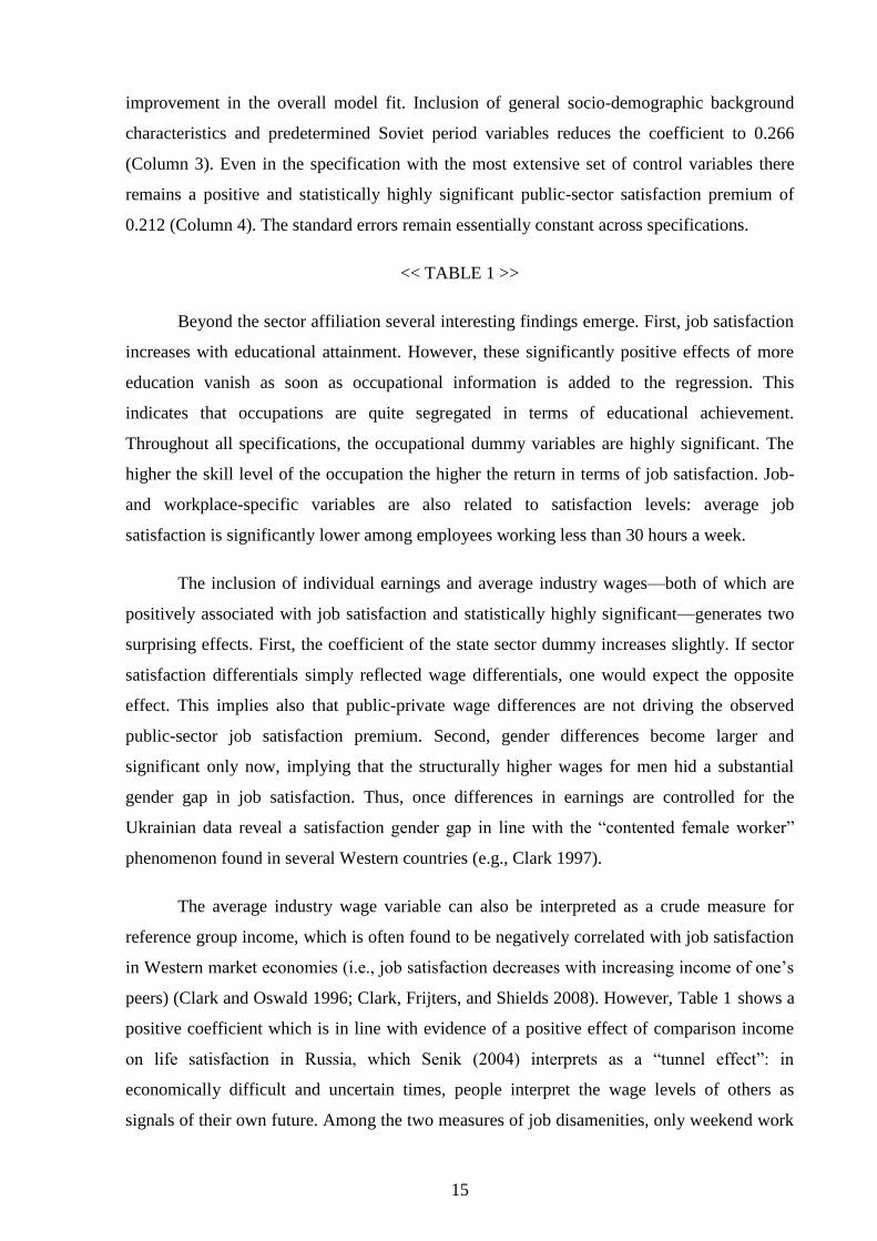
improvement in the overall model fit. Inclusion of general socio-demographic background
characteristics and predetermined Soviet period variables reduces the coefficient to 0.266
(Column 3). Even in the specification with the most extensive set of control variables there
remains a positive and statistically highly significant public-sector satisfaction premium of
0.212 (Column 4). The standard errors remain essentially constant across specifications.
<< TABLE 1 >>
Beyond the sector affiliation several interesting findings emerge. First, job satisfaction
increases with educational attainment. However, these significantly positive effects of more
education vanish as soon as occupational information is added to the regression. This
indicates that occupations are quite segregated in terms of educational achievement.
Throughout all specifications, the occupational dummy variables are highly significant. The
higher the skill level of the occupation the higher the return in terms of job satisfaction. Job-
and workplace-specific variables are also related to satisfaction levels: average job
satisfaction is significantly lower among employees working less than 30 hours a week.
The inclusion of individual earnings and average industry wages—both of which are
positively associated with job satisfaction and statistically highly significant—generates two
surprising effects. First, the coefficient of the state sector dummy increases slightly. If sector
satisfaction differentials simply reflected wage differentials, one would expect the opposite
effect. This implies also that public-private wage differences are not driving the observed
public-sector job satisfaction premium. Second, gender differences become larger and
significant only now, implying that the structurally higher wages for men hid a substantial
gender gap in job satisfaction. Thus, once differences in earnings are controlled for the
Ukrainian data reveal a satisfaction gender gap in line with the “contented female worker”
phenomenon found in several Western countries (e.g., Clark 1997).
The average industry wage variable can also be interpreted as a crude measure for
reference group income, which is often found to be negatively correlated with job satisfaction
in Western market economies (i.e., job satisfaction decreases with increasing income of one’s
peers) (Clark and Oswald 1996; Clark, Frijters, and Shields 2008). However, Table 1 shows a
positive coefficient which is in line with evidence of a positive effect of comparison income
on life satisfaction in Russia, which Senik (2004) interprets as a “tunnel effect”: in
economically difficult and uncertain times, people interpret the wage levels of others as
signals of their own future. Among the two measures of job disamenities, only weekend work
16
is significantly negatively related to job satisfaction. Regarding the proxies for personality
traits and risk aversion, only the coefficient for extroverted types is significantly positive.
4.2 Results from the IV Regressions
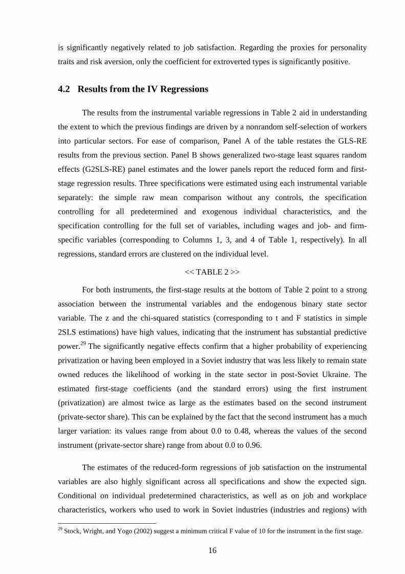
The results from the instrumental variable regressions in Table 2 aid in understanding
the extent to which the previous findings are driven by a nonrandom self-selection of workers
into particular sectors. For ease of comparison, Panel A of the table restates the GLS-RE
results from the previous section. Panel B shows generalized two-stage least squares random
effects (G2SLS-RE) panel estimates and the lower panels report the reduced form and first-
stage regression results. Three specifications were estimated using each instrumental variable
separately: the simple raw mean comparison without any controls, the specification
controlling for all predetermined and exogenous individual characteristics, and the
specification controlling for the full set of variables, including wages and job- and firm-
specific variables (corresponding to Columns 1, 3, and 4 of Table 1, respectively). In all
regressions, standard errors are clustered on the individual level.
<< TABLE 2 >>
For both instruments, the first-stage results at the bottom of Table 2 point to a strong
association between the instrumental variables and the endogenous binary state sector
variable. The z and the chi-squared statistics (corresponding to t and F statistics in simple
2SLS estimations) have high values, indicating that the instrument has substantial predictive
power.29
The significantly negative effects confirm that a higher probability of experiencing
privatization or having been employed in a Soviet industry that was less likely to remain state
owned reduces the likelihood of working in the state sector in post-Soviet Ukraine. The
estimated first-stage coefficients (and the standard errors) using the first instrument
(privatization) are almost twice as large as the estimates based on the second instrument
(private-sector share). This can be explained by the fact that the second instrument has a much
larger variation: its values range from about 0.0 to 0.48, whereas the values of the second
instrument (private-sector share) range from about 0.0 to 0.96.
The estimates of the reduced-form regressions of job satisfaction on the instrumental
variables are also highly significant across all specifications and show the expected sign.
Conditional on individual predetermined characteristics, as well as on job and workplace
characteristics, workers who used to work in Soviet industries (industries and regions) with
29
Stock, Wright, and Yogo (2002) suggest a minimum critical F value of 10 for the instrument in the first stage.
17
more privatizations (instrument 1) or general restructuring (instrument 2) report lower levels
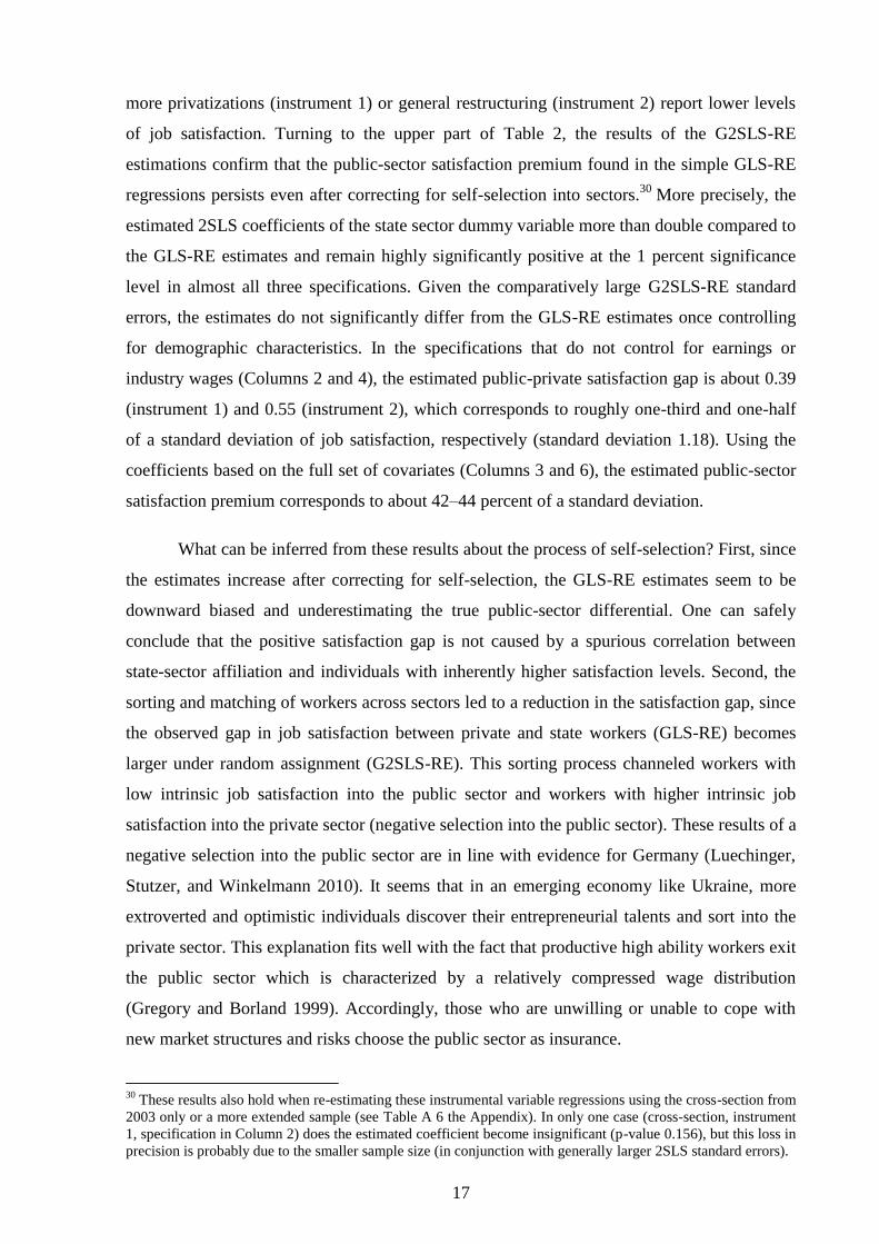
of job satisfaction. Turning to the upper part of Table 2, the results of the G2SLS-RE
estimations confirm that the public-sector satisfaction premium found in the simple GLS-RE
regressions persists even after correcting for self-selection into sectors.30
More precisely, the
estimated 2SLS coefficients of the state sector dummy variable more than double compared to
the GLS-RE estimates and remain highly significantly positive at the 1 percent significance
level in almost all three specifications. Given the comparatively large G2SLS-RE standard
errors, the estimates do not significantly differ from the GLS-RE estimates once controlling
for demographic characteristics. In the specifications that do not control for earnings or
industry wages (Columns 2 and 4), the estimated public-private satisfaction gap is about 0.39
(instrument 1) and 0.55 (instrument 2), which corresponds to roughly one-third and one-half
of a standard deviation of job satisfaction, respectively (standard deviation 1.18). Using the
coefficients based on the full set of covariates (Columns 3 and 6), the estimated public-sector
satisfaction premium corresponds to about 42–44 percent of a standard deviation.
What can be inferred from these results about the process of self-selection? First, since
the estimates increase after correcting for self-selection, the GLS-RE estimates seem to be
downward biased and underestimating the true public-sector differential. One can safely
conclude that the positive satisfaction gap is not caused by a spurious correlation between
state-sector affiliation and individuals with inherently higher satisfaction levels. Second, the
sorting and matching of workers across sectors led to a reduction in the satisfaction gap, since
the observed gap in job satisfaction between private and state workers (GLS-RE) becomes
larger under random assignment (G2SLS-RE). This sorting process channeled workers with
low intrinsic job satisfaction into the public sector and workers with higher intrinsic job
satisfaction into the private sector (negative selection into the public sector). These results of a
negative selection into the public sector are in line with evidence for Germany (Luechinger,
Stutzer, and Winkelmann 2010). It seems that in an emerging economy like Ukraine, more
extroverted and optimistic individuals discover their entrepreneurial talents and sort into the
private sector. This explanation fits well with the fact that productive high ability workers exit
the public sector which is characterized by a relatively compressed wage distribution
(Gregory and Borland 1999). Accordingly, those who are unwilling or unable to cope with
new market structures and risks choose the public sector as insurance.
30
These results also hold when re-estimating these instrumental variable regressions using the cross-section from
2003 only or a more extended sample (see Table A 6 the Appendix). In only one case (cross-section, instrument
1, specification in Column 2) does the estimated coefficient become insignificant (p-value 0.156), but this loss in
precision is probably due to the smaller sample size (in conjunction with generally larger 2SLS standard errors).
18
What can be learned about the role of equalizing differentials in total compensation in
post-Soviet Ukraine? Following the considerations in Section 2, the estimated satisfaction
premium of state-sector employees indicates a larger fraction of unsatisfied workers in the
private than in the public sector. Against the background of a continuously shrinking state
sector, this satisfaction gap is indicative for an increasing “shortage” of public-sector jobs for
which more and more private-sector workers queue as they would be better off. Hence, the
satisfaction premium indeed represents a rent that one person receives by working in the state
rather than the private sector. Reducing (increasing) total remuneration (monetary and non-
monetary) in the public (private) sector should lower the satisfaction differential.
4.3 Sensitivity and robustness checks
4.3.1 Excluding recent privatizations
The identifying assumption of the empirical strategy requires that the instrument (the
ex-ante privatization probability) in itself does not directly affect today’s job satisfaction
(exclusion restriction). Although it is not possible to actually prove this condition, it is
possible to provide suggestive evidence in support of the validity of the instruments. First,
contrary to the general public notion that privatization hurts workers, Brown, Earle and
Vakhitov (2006) and Brown, Earle and Telegdy (2010) show for Ukraine and other transition
countries that privatization did not lead to job losses and had either only very small or no
effects on wages (in fact, in some cases privatization even caused an increase in firm
employment and wages). Second, managerial turnover (on higher management levels) that
could potentially trigger unpleasant organizational change or a general restructuring of firms
and thus might lower job satisfaction was actually less common in de novo or privatized firms
than in state-owned enterprises (see Warzynski 2003 using a sample of 300 Ukrainian firms in
1997). Warzynski (2003) explains this finding by the fact that the particular privatization
process in Ukraine predominantly led to insider ownership (by workers and managers). Third,
general changes in the economic and political system during the transition process, e.g., more
competitive pressure from foreign firms, liberalization of consumer prices, would affect all
employees in Ukraine. Debardeleben (1999) analyses the attitudes of Russians towards the
privatization process based on Russian survey data from 1993 to 1997. Individuals with
personal privatization experiences are neither more nor less supportive of the privatization
process and market liberalizations than persons without such personal privatization
experience. The author concludes that disillusion with the political process and market
19
transition as a whole led to a general negative assessment of single transition measures in the
population. If similar mechanisms have taken place in Ukraine this would furthermore support
the notion that privatization in itself did not affect satisfaction levels of individuals.
Additionally, it is possible to perform a simple test on whether the main estimation
results are driven by recent – and possibly unpleasant – privatization experiences of some
ULMS participants. If privatization has a direct negative effect on job satisfaction, this effect
should be strongest immediately around or after the date of privatization and should gradually
fade out over time. This is why the main G2SLS-RE regressions from Table 2 are repeated
after dropping all observations that have experienced privatization within the last four years
preceding the survey. Panel A in Table 3 indicates that the estimated state sector premium
does not diminish after excluding these recent privatizations.31
In contrary, the estimates
become even slightly larger thereby lending further support to the claim that the main
regression results are not driven by possibly negative privatization experiences of workers.
<< TABLE 3 >>
4.3.2 Excluding ‘social Soviet jobs’ and extreme IV values
If Soviet workers actually could and did self-select into specific occupations and
industries and if particular types of individuals (happy types) were attracted to ‘typical
Western’ public sector jobs even in the Soviet Union (e.g., public administration, education,
health) the validity of the instrumental variables would be in jeopardy. However, employees
in the Soviet public administration, education or health care system (typically dominated by
white-collar occupations) did not benefit from additional job amenities (like job security)
which are typically attributed to public sector jobs in Western market economies. Hence, any
self-selection of workers into ‘typical’ public sector industries on the basis of job
characteristics which are commonly ascribed to Western public sector jobs (e.g. job amenities,
job security) can be excluded. In fact, in the 1980s skilled manual workers received an official
wage premium thereby earning more than managers and some professionals (Gerber and Hout
2004). Furthermore, Soviet workers in blue-collar occupations generally benefited from better
working conditions and incentives – much in line with Soviet ideology and its emphasis on
manual labor (Zajda 1980). This ideologically motivated preferential treatment of blue collar
workers (i.e. not ‘typical public sector’ jobs) works against the idea that Soviet workers
selected into ‘typical public sector’ industries due to beneficial job attributes.
31
These results hold also when excluding only individuals having experienced privatization within the last, the
last two or the last three years (results not reported).
20
To find out whether the state sector satisfaction premium is merely caused by socially
oriented personality types, Panel B of Table 3 presents results after excluding all individuals
who used to work in ‘typical social’ jobs during the Soviet time. The problem with this
approach is that it is theoretically possible that people enjoy doing social or service work and
that this type of job content might actually represent job amenities leading to higher job
satisfaction. Individuals are classified as ‘Soviet social job’ holders based on their Soviet 4-
digit ISCO occupational codes whenever these are related to education, health and safety
services, social and social security workers (overall 58 different occupations). Excluding these
observations from the sample tends to reduce the estimated public sector premium coefficient
as well as the significance level slightly. However, the previous findings of a significantly
positive job satisfaction premium of state sector workers are confirmed, suggesting that the
positive effect of working in the public sector is not driven by socially oriented worker types.
Panel C of Table 3 shows that the results are also robust to excluding the smallest and
largest values of the instrumental variables. By dropping the observations at the bottom and
the top 5 % of the instrumental variable distribution, this robustness checks makes sure that
the main results are not driven by industries (and regions) with the lowest or the highest
privatization probabilities (at the bottom these are education and public administration).
4.3.3 Using only ‘industry stayers’
As the instrumental variables are assigned to workers’ Soviet industry affiliations, they
should be more powerful for individuals who remained in the same industry since Soviet
times (workers might have changed jobs or firms within the same industry). Since this
subsample of workers might generally differ from those workers who have switched
industries, it is problematic to run the regression on this selected sample. Nevertheless, this
exercise should help to test whether the instrument is ‘functioning’ in the right way, i.e.
whether results become more precise despite a smaller sample size. The reassuring results in
Panel D of Table 3 show that this is indeed the case: while the point estimates change slightly,
the standard errors become smaller and the estimated coefficients are all highly significant.
The first stage becomes stronger (results not shown).
5 The Role of Fringe Benefits and Job Security
If the state sector satisfaction premium is not caused by self-selection of workers, why
are public sector workers on average more satisfied with their jobs? How important are
21
differences in job amenities? The ULMS allows an assessment of the importance of two
different types of amenity: perceived job security and fringe benefits.
The ULMS waves 2004 and 2007 contain a subjective measure of job security: Tell
me, please, how satisfied are you with your current job in terms of job security? The five
answer possibilities range from fully dissatisfied (=1) to fully satisfied (=5). Table 4 reports
the effect of working in the state sector on satisfaction with job security. Across all
specifications and instrumental variables the estimated effects are strikingly large (larger than
in the job satisfaction regressions) and positively significant implying a substantial
satisfaction premium in terms of job security in the state sector (even after correcting for self-
selection into the public and private sector). The coefficients range between 0.54 and 0.90 of a
standard deviation. These results seem to indicate that public sector jobs in the Ukraine are
indeed perceived as more secure than private sector jobs and that this job facet might be a part
of the overall public sector job satisfaction premium.
<< TABLE 4 >>
Regarding fringe benefits, the ULMS asks respondents a long battery of questions on
provision of social benefits and financial incentive schemes by the employer. The question on
social benefits is workplace rather than person specific: In this job do employees receive any
of the following social benefits? Thus, part of the individual-level endogeneity problem (if
benefit receipt within firms was heterogeneous) is alleviated, although it is still possible that
workers sort into particular companies offering these types of job amenities. To reduce the
dimensionality and complexity of the information, the 13 social benefits were grouped into
three categories: social security (e.g., regular paid vacation, paid sick leave), subsidies (e.g.,
free childcare, discounted food, transportation or housing subsidies), and training (e.g.,
human-capital enhancing measures like paid training or payment for trips to sanatoria). The
information on financial benefits is based on the question as to whether respondents received
any amount of money in addition to their regular salary in the past year. Since receipt of this
additional money is measured at the individual level, the problem of endogeneity is more
pronounced. Three different types of payments are distinguished: non-performance-related
benefits (i.e., 13th
salary), performance-related benefits (bonus payments or profit-sharing
payment schemes), and risk compensation (compensation for non-normal work conditions).
A first descriptive analysis, set out in Table 5, demonstrates that both social benefits
and financial benefits are much more common in the state than in the private sector. For
instance, almost all state-sector (97 percent) but only 61 percent of private sector employees
22
report that their workplace provides them with at least one of the following social security
type of benefits: regular paid vacation, paid sick leave, paid maternity leave/childcare leave,
and coverage of health-related expenses (or treatment in at the enterprise’s clinic). The same
pattern is found in the provision of training or subsidy type of benefits. It is important to note
that these types of social benefits were generally available to all workers during the Soviet
period—irrespective of their industry or occupation. Against this background, the post-Soviet
discrepancy in provision of these benefits between both sectors is even more striking.
<< TABLE 5 >>
To analyze whether the estimated public job satisfaction premium can be explained by
the variation in benefits across sectors, the GLS-RE and G2SLS-RE regressions from Section
4 are extended by successively including sets of dummy variables for different types of
benefits (only social benefits, only financial benefits, both types of benefits). Several
interesting findings emerge. First, adding controls for the provision of fringe benefits reduces
the size of the estimated GLS-RE coefficients of the state sector dummy variable (Table 6,
Columns 1 to 3). While the GLS-RE state-sector coefficient in the full regression
specification was 0.211, it drops to 0.141 once all types of benefits are included in the
regression. In the GLS-RE regressions, the coefficients on social benefits as well as pay
schemes show the expected positive sign and are significantly different from zero. However,
despite the inclusion of these variables, there remains an unexplained positive satisfaction
gap. Second, rerunning the regression with G2SLS-RE reveals the same pattern: the estimated
coefficients drop in size, but remain significant. In summary, the public-private job
satisfaction differential can be partly related to the different levels of social and financial
fringe benefits in the two sectors. However, the explanatory power of these non-wage
components of total compensation is limited, since two third of the public-sector premium
remain even after controlling for these types of benefits.
<< TABLE 6 >>
6 Conclusions
This paper analyzes differences in job satisfaction between public- and private-sector
employees. The main contribution is to disentangle the raw public-private sector satisfaction
gap observed in Ukraine into a part reflecting self-selection of workers according to
unobserved heterogeneity (i.e., personality types) and a remainder driven by genuine
differences in job characteristics (i.e., rents in the public sector). This study is the first to
23
address this particular problem using a natural experiment. The identification strategy exploits
the quasi-experiment generated by the fundamental changes in ownership of enterprises made
during Ukraine’s transition to a market economy, during which workers were randomly
reallocated from state- to private-sector jobs.
The empirical results reveal that the significantly positive public-sector satisfaction
premium holds even after correcting for self-selection. Against the background of the theory
of equalizing differentials, these results indicate rents received by public-sector employees in
Ukraine. The findings are robust to several sensitivity tests. Accounting and correcting for the
nonrandom sorting into state and private sector leads to an increase in the size of the
satisfaction gap. This suggests a negative selection of workers into the public sector. An
important conclusion of the analysis is that rents of public workers might be underestimated
when not correcting for self-selection or when only looking at wages. The same pattern of
negative selection is found for Germany using structural switching regression models
(Luechinger, Stutzer, and Winkelmann 2010). However, the results are in contrast with those
of Heywood et al. (2002), who find a positive selection into public-sector employment in the
United Kingdom based on panel fixed effects estimations.
Assessing the potential drivers of the public-private satisfaction differential revealed
that a certain fraction of the state-sector premium can be explained by different fringe benefits
in the two sectors. However, as the significant public-sector satisfaction premium remains
even after controlling for fringe benefits and self-selection, open questions remain regarding
additional factors explaining the gap. These could include, for instance, sector differences in
job and time flexibility (including formal as well as informal rules, e.g., specific firm culture
and attitudes) or differences in wage compression across sectors, which would matter if
individuals cared about wage inequality and relative wages within firms. Another explanation
could be differences in perceived job and income uncertainty in the two sectors. In fact, the
analysis revealed that public-sector employees are more satisfied with job security than their
private-sector counterparts. In the absence of well-functioning financial markets, public-sector
employment could act as an insurance mechanism and be thus especially valued by
individuals (Rodrik 2000). Furthermore, public-sector rents could also be related to unofficial
payments or bribes to public-sector employees. Indeed, Gorodnichenko and Sabirianova Peter
(2007) point towards the existence of bribery in Ukraine. Having established the causality of
the public-sector job satisfaction premium and having investigated one potential source of
satisfaction difference (fringe benefits), this paper leaves the study of other job attributes
which potentially drive the public-sector satisfaction premium for future research.
24
7 References
Angrist, Joshua D. 2001. “Estimation of Limited Dependent Variable Models with Dummy
Endogenous Regressors: Simple Strategies for Empirical Practice.” Journal of
Business & Economic Statistics, 19 (1): 2–16.
Ashenfelter, Orley. 1978. “Estimating the Effect of Training Programs on Earnings.” Review
of Economics and Statistics, 60 (1): 47–57.
Belfield, Clive R. and R.D.F. Harris. 2002. “How Well Do Theories of Job Matching
Explain Variations in Job Satisfaction Across Education Levels? Evidence for UK
Graduates.” Applied Economics, 34 (5): 535–548.
Blank, Rebecca M. 1985. “An Analysis of Workers’ Choice Between Employment in the
Public and Private Sectors.” Industrial and Labor Relations Review, 38 (2): 211–224.
Boswell, Wendy R., John W. Boudreau, and Jan Tichy. 2005. “The Relationship Between
Employee Job Change and Job Satisfaction: The Honeymoon–Hangover Effect.”
Journal of Applied Psychology, 90 (5): 882–892.
Brown, David J., John S. Earle, and Álmos Telegdy. 2006. “The Productivity Effects of
Privatization: Longitudinal Estimates from Hungary, Romania, Russia and Ukraine.”
Journal of Political Economy, 114 (2): 61–99.
Brown, David J., John S. Earle, and Álmos Telegdy. 2010. “Employment and Wage
Effects of Privatisation: Evidence from Hungary, Romania, Russia and Ukraine.”
Economic Journal, 120 (545): 683–708.
Brown, David J., John S. Earle, and Volodymyr Vakhitov. 2006. “Wages, Layoffs, and
Privatization: Evidence from Ukraine.” Journal of Comparative Economics, 34 (2):
272–294.
Brown, Emily Clark. 1973. “Fundamental Soviet Labor Legislation.” Industrial and Labor
Relations Review, 26 (2): 778–792.
Clark, Andrew. 1997. “Job Satisfaction and Gender: Why Are Women So Happy at Work?”
Labour Economics, 4 (4): 341–372.
Clark, Andrew E., Ed Diener, Yannis Georgellis, and Richard E. Lucas. 2008. “Lags and
Leads in Life Satisfaction: A Test of the Baseline Hypothesis.” Economic Journal, 118
(529): F222–F243.
25
Clark, Andrew E., Paul Frijters, and Michael A. Shields. 2008. “Relative Income,
Happiness, and Utility: An Explanation for the Easterlin Paradox and Other Puzzles.”
Journal of Economic Literature, 46 (1): 95–144.
Clark, Andrew E. and Andrew J. Oswald. 1996. “Satisfaction and Comparison Income.”
Journal of Public Economics, 61 (3): 359–381.
Clark, Andrew E. and Claudia Senik. 2006. “The (Unexpected) Structure of ‘Rents’ on the
French and British Labour Markets.” Journal of Socio-Economics, 35 (2): 180–196.
Danzer, Alexander M. and Peter J. Dolton. 2012. “Total Reward and Pensions in the UK in
the Public and Private Sectors.” Labour Economics, 19 (4): 584-594.
Demoussis, Michael and Nicholas Giannakopoulos. 2007. “Exploring Job Satisfaction in
Private and Public Employment: Empirical Evidence from Greece.” Labour, 21 (2):
333–359.
Ehrenberg, Ronald G. and Joshua L. Schwarz. 1987.“Public Sector Labor Markets.” In:
Ashenfelter, Orley C. and Richard Layard (eds.), Handbook of Labor Economics,
Elsevier, Volume 2, part 2, chapter 22: 1219–1260.
Estrin, Saul, Jan Hanousek, Evzen Kocenda, and Jan Svejnar. 2009. “The Effects of
Privatization and Ownership in Transition Economies.” Journal of Economic
Literature, 47 (3): 699–728.
Ferrer-i-Carbonell, Ada and Paul Frijters. 2004.“How Important is Methodology for the
Estimates of the Determinants of Happiness?” Economic Journal, 114 (497): 641–659.
Flemming, John S. and John Micklewright. 2000. “Income Distribution, Economic
Systems and Transition.” In: Atkinson, Anthony B. and Francois Bourguignon (eds.),
Handbook of Income Distribution, Elsevier, volume 1, chapter 14: 843–918.
Friebel, Guido and Sergei Guriev. 2005. “Attaching Workers Through In-Kind Payments:
Theory and Evidence from Russia.” World Bank Economic Review, 19 (2): 175–202.
Frijters, Paul, Ingo Geishecker, John Haisken-DeNew, and Michael A. Shields. 2006.
“Can the Large Swings in Russian Life Satisfaction be Explained by Ups and Downs
in Real Incomes?” Scandinavian Journal of Economics, 108 (3): 433–458.
Fuchs-Schündeln, Nicola and Matthias Schündeln. 2005.“Precautionary Savings and Self-
Selection: Evidence from the German Reunification ‘Experiment’.” Quarterly Journal
of Economics, 120 (3): 1085–1120.
26
Ganguli, Ina and Katherine Terrell. 2006. “Institutions, Markets and Men’s and Women’s
Wage Inequality: Evidence from Ukraine.” Journal of Comparative Economics, 34
(2): 200–227.
Ghinetti, Paolo. 2007.“The Public–Private Job Satisfaction Differential in Italy.” Labour, 21
(2): 361–388.
Gibbons, Robert and Lawrence F. Katz. 1992. “Does Unmeasured Ability Explain Inter-
Industry Wage Differentials?” Review of Economic Studies, 59 (3): 515–535.
Gorodnichenko, Yurij and Klara Sabirianova Peter. 2007. “Public Sector Pay and
Corruption: Measuring Bribery from Micro Data.” Journal of Public Economics, 91
(5–6): 963–991.
Gregory, Paul R. and Irwin L. Collier. 1988. “Unemployment in the Soviet Union:
Evidence from the Soviet Interview Project.” American Economic Review, 78 (4):
613–632.
Gregory, Paul R. and Janet E. Kohlhase. 1988. “The Earnings of Soviet Workers: Evidence
from the Soviet Interview Project.” Review of Economics and Statistics, 70 (1): 23–35.
Gregory, Robert G. and Jeff Borland. 1999. “Recent Developments in Public Sector
Markets.” In: Ashenfelter, Orley C. and David Card (eds.), Handbook of Labor
Economics, Elsevier, volume 3, part 3, chapter 53: 3573–3630.
Grygorenko, Galyna and Stefan Lutz. 2007. “Firm Performance and Privatization in
Ukraine.” Economic Change and Restructuring, 40 (3):253–266.
Haddad, L. 1972. “Wages in the Soviet Union: Problems of Policy.” Journal of Industrial
Relations, 14 (2): 171–174.
Hamermesh, Daniel S. 1999. “Changing Inequality in Markets for Workplace Amenities.”
Quarterly Journal of Economics, 114 (4): 1085–1123.
Hamermesh, Daniel S. 2001.“The Changing Distribution of Job Satisfaction.” Journal of
Human Resources, 36 (1): 1–30.
Helliwell, John and Haifang Huang. 2010. “How’s the Job? Well-Being and Social Capital
in the Workplace.” Industrial and Labor Relations Review, 63(2): Article 2.
Heywood, John S., W. S. Siebert, and Xiangdong Wei. 2002. “Worker Sorting and Job
Satisfaction: The Case of Union and Government Jobs.” Industrial and Labor
Relations Review, 55(4): 595–609.
27
Imbens, Guido W. and Joshua D. Angrist. 1994. “Identification and Estimation of Local
Average Treatment Effects.” Econometrica, 62 (2): 467–475.
Katz, Lawrence F. and David H. Autor. 1999. “Changes in the Wage Structure and
Earnings Inequality.” In: Card, David (ed.), Handbook of Labor Economics, Elsevier,
volume 3A, 1463–1555.
Krueger, Alan B. 1988. “The Determinants of Queues for Federal Jobs.” Industrial and
Labor Relations Review, 41(4): 567–581.
Luechinger, Simon, Stephan Meier, and Alois Stutzer. 2008. “Bureaucratic Rents and Life
Satisfaction.” Journal of Law, Economics, and Organization, 24 (2): 476–488.
Luechinger, Simon, Stephan Meier, and Alois Stutzer. 2010. “Why Does Unemployment
Hurt the Employed? Evidence from the Life Satisfaction Gap Between the Public and
the Private Sector.” Journal of Human Resources, 45 (4): 998–1045.
Luechinger, Simon, Alois Stutzer, and Rainer Winkelmann. 2006. “The Happiness Gains
from Sorting and Matching in the Labor Market.” IZA discussion paper, No. 2019.
Luechinger, Simon, Alois Stutzer, and Rainer Winkelmann. 2010. “Self-Selection Models
for Public and Private Sector Job Satisfaction.” Research in Labor Economics, 30
(30): 233–251.
Megginson, William L. and Jeffry M. Netter. 2001. “From State to Market: A Survey of
Empirical Studies on Privatization.” Journal of Economic Literature, 39 (2): 321–389.
Pivovarsky, Alexander. 2001. “How Does Privatization Work? Ownership Concentration
and Enterprise Performance in Ukraine.” IMF working paper, No. WP/01/42.
Rodrik, Dani. 2000. “What Drives Public Employment in Developing Countries?” Review of
Development Economics, 4 (3): 229–243.
Rosen, Sherwin. 1987. “The Theory of Equalizing Differences.” In: Ashenfelter, Orley C.
and Richard Layard (eds.), Handbook of Labor Economics, Elsevier, edition 1, volume
1, part 1, chapter 12: 641–692.
Senik, Claudia. 2004. “When Information Dominates Comparison—Learning from Russian
Subjective Panel Data.” Journal of Public Economics, 88 (9–10): 2099–2123.
State Statistics Committee of Ukraine. 2005. Statistical Yearbook of Ukraine 2004. Kiev,
Ukraine.
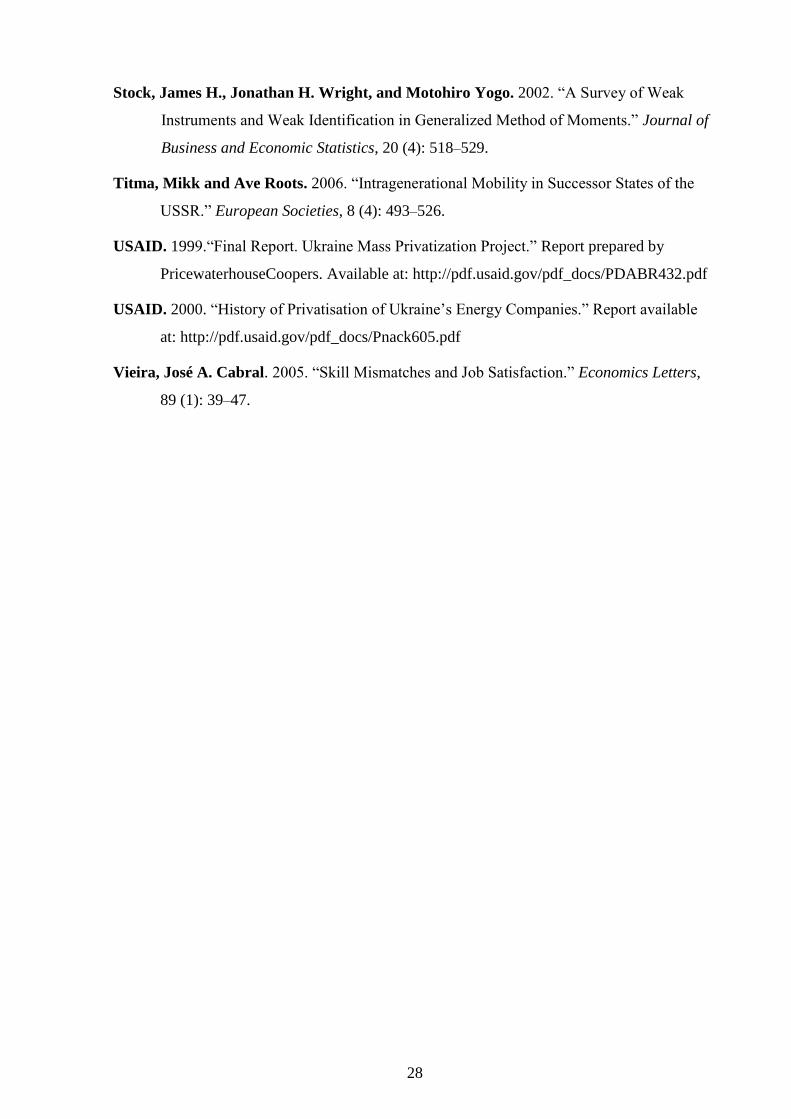
28
Stock, James H., Jonathan H. Wright, and Motohiro Yogo. 2002. “A Survey of Weak
Instruments and Weak Identification in Generalized Method of Moments.” Journal of
Business and Economic Statistics, 20 (4): 518–529.
Titma, Mikk and Ave Roots. 2006. “Intragenerational Mobility in Successor States of the
USSR.” European Societies, 8 (4): 493–526.
USAID. 1999.“Final Report. Ukraine Mass Privatization Project.” Report prepared by
PricewaterhouseCoopers. Available at: http://pdf.usaid.gov/pdf_docs/PDABR432.pdf
USAID. 2000. “History of Privatisation of Ukraine’s Energy Companies.” Report available
at: http://pdf.usaid.gov/pdf_docs/Pnack605.pdf
Vieira, José A. Cabral. 2005. “Skill Mismatches and Job Satisfaction.” Economics Letters,
89 (1): 39–47.
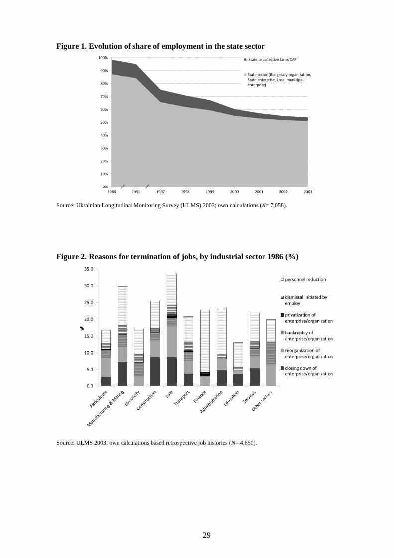
29
Figure 1. Evolution of share of employment in the state sector
Source: Ukrainian Longitudinal Monitoring Survey (ULMS) 2003; own calculations (N= 7,058).
Figure 2. Reasons for termination of jobs, by industrial sector 1986 (%)
Source: ULMS 2003; own calculations based retrospective job histories (N= 4,650).
0%
10%
20%
30%
40%
50%
60%
70%
80%
90%
100%
1986 1991 1997 1998 1999 2000 2001 2002 2003
State or collective farm/CAP
State sector (Budgetary organization,State enterprise, Local municipalenterprise)
0.0
5.0
10.0
15.0
20.0
25.0
30.0
35.0
%
personnel reduction
dismissal initiated byemploy
privatization ofenterprise/organization
bankruptcy ofenterprise/organization
reorganization ofenterprise/organization
closing down ofenterprise/organization

30
Figure 3. Job satisfaction in the private and public sector in Ukraine
Source: ULMS 2003–2007, pooled sample of all individuals of working age with retrospective Soviet job information
(extended regression sample; N=5,142); own calculations.
12.3
16.6
23.6
32.7
14.8
6.5
12.1
22.6
38.8
19.9
0
5
10
15
20
25
30
35
40
45
Fully dissatisfied Rather dissatisfied Neither satisfied, nordissatisfied
Rather satisfied Fully satisfied
% in
re
spe
ctiv
e se
cto
r
Private sector
State sector
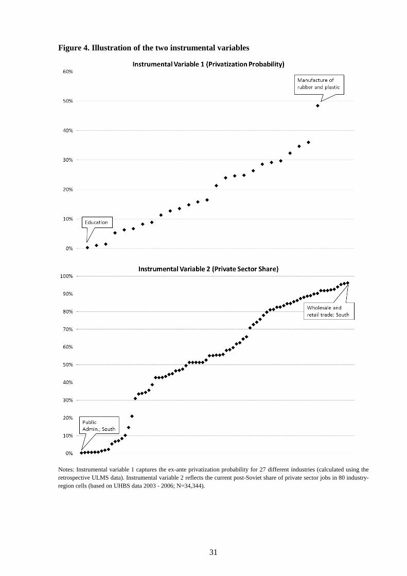
31
Figure 4. Illustration of the two instrumental variables
Notes: Instrumental variable 1 captures the ex-ante privatization probability for 27 different industries (calculated using the
retrospective ULMS data). Instrumental variable 2 reflects the current post-Soviet share of private sector jobs in 80 industry-
region cells (based on UHBS data 2003 - 2006; N=34,344).
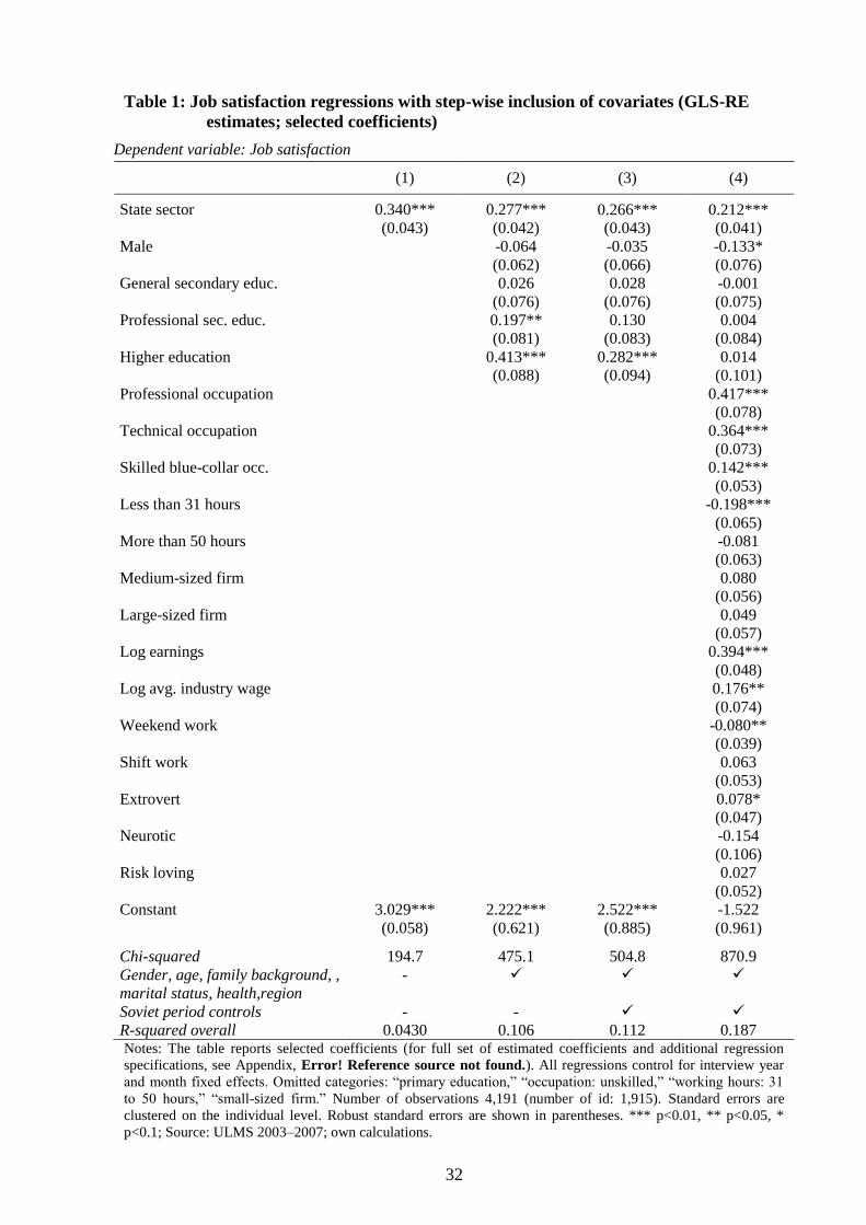
32
Table 1: Job satisfaction regressions with step-wise inclusion of covariates (GLS-RE
estimates; selected coefficients)
Dependent variable: Job satisfaction
(1) (2) (3) (4)
State sector 0.340*** 0.277*** 0.266*** 0.212***
(0.043) (0.042) (0.043) (0.041)
Male -0.064 -0.035 -0.133*
(0.062) (0.066) (0.076)
General secondary educ. 0.026 0.028 -0.001
(0.076) (0.076) (0.075)
Professional sec. educ. 0.197** 0.130 0.004
(0.081) (0.083) (0.084)
Higher education 0.413*** 0.282*** 0.014
(0.088) (0.094) (0.101)
Professional occupation 0.417***
(0.078)
Technical occupation 0.364***
(0.073)
Skilled blue-collar occ. 0.142***
(0.053)
Less than 31 hours -0.198***
(0.065)
More than 50 hours -0.081
(0.063)
Medium-sized firm 0.080
(0.056)
Large-sized firm 0.049
(0.057)
Log earnings 0.394***
(0.048)
Log avg. industry wage 0.176**
(0.074)
Weekend work -0.080**
(0.039)
Shift work 0.063
(0.053)
Extrovert 0.078*
(0.047)
Neurotic -0.154
(0.106)
Risk loving 0.027
(0.052)
Constant 3.029*** 2.222*** 2.522*** -1.522
(0.058) (0.621) (0.885) (0.961)
Chi-squared 194.7 475.1 504.8 870.9
Gender, age, family background, ,
marital status, health,region
-
Soviet period controls - -
R-squared overall 0.0430 0.106 0.112 0.187 Notes: The table reports selected coefficients (for full set of estimated coefficients and additional regression
specifications, see Appendix, Error! Reference source not found.). All regressions control for interview year
and month fixed effects. Omitted categories: “primary education,” “occupation: unskilled,” “working hours: 31
to 50 hours,” “small-sized firm.” Number of observations 4,191 (number of id: 1,915). Standard errors are
clustered on the individual level. Robust standard errors are shown in parentheses. *** p<0.01, ** p<0.05, *
p<0.1; Source: ULMS 2003–2007; own calculations.
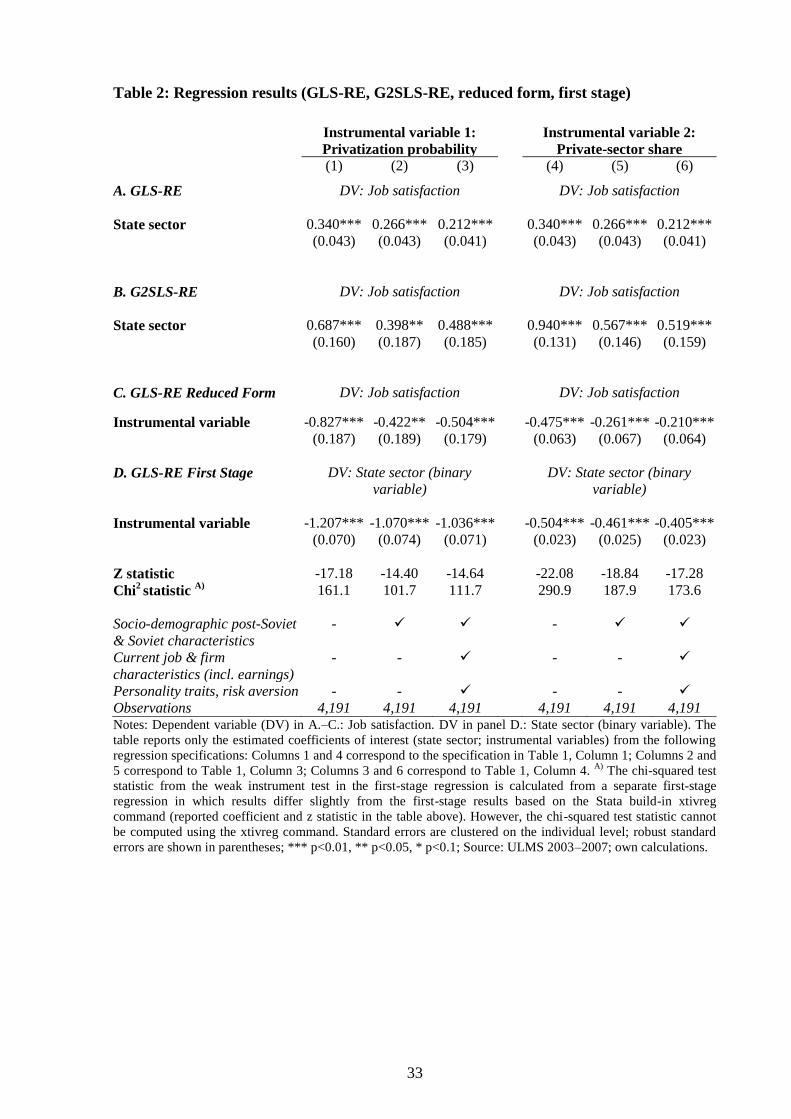
33
Table 2: Regression results (GLS-RE, G2SLS-RE, reduced form, first stage)
Instrumental variable 1:
Privatization probability
Instrumental variable 2:
Private-sector share
(1) (2) (3) (4) (5) (6)
A. GLS-RE DV: Job satisfaction
DV: Job satisfaction
State sector 0.340*** 0.266*** 0.212*** 0.340*** 0.266*** 0.212***
(0.043) (0.043) (0.041) (0.043) (0.043) (0.041)
B. G2SLS-RE DV: Job satisfaction
DV: Job satisfaction
State sector 0.687*** 0.398** 0.488*** 0.940*** 0.567*** 0.519***
(0.160) (0.187) (0.185) (0.131) (0.146) (0.159)
C. GLS-RE Reduced Form DV: Job satisfaction DV: Job satisfaction
Instrumental variable -0.827*** -0.422** -0.504*** -0.475*** -0.261*** -0.210***
(0.187) (0.189) (0.179) (0.063) (0.067) (0.064)
D. GLS-RE First Stage DV: State sector (binary
variable)
DV: State sector (binary
variable)
Instrumental variable -1.207*** -1.070*** -1.036*** -0.504*** -0.461*** -0.405***
(0.070) (0.074) (0.071) (0.023) (0.025) (0.023)
Z statistic -17.18 -14.40 -14.64 -22.08 -18.84 -17.28
Chi2 statistic
A) 161.1 101.7 111.7 290.9 187.9 173.6
Socio-demographic post-Soviet
& Soviet characteristics
- -
Current job & firm
characteristics (incl. earnings)
- - - -
Personality traits, risk aversion - - - -
Observations 4,191 4,191 4,191 4,191 4,191 4,191 Notes: Dependent variable (DV) in A.–C.: Job satisfaction. DV in panel D.: State sector (binary variable). The
table reports only the estimated coefficients of interest (state sector; instrumental variables) from the following
regression specifications: Columns 1 and 4 correspond to the specification in Table 1, Column 1; Columns 2 and
5 correspond to Table 1, Column 3; Columns 3 and 6 correspond to Table 1, Column 4. A)
The chi-squared test
statistic from the weak instrument test in the first-stage regression is calculated from a separate first-stage
regression in which results differ slightly from the first-stage results based on the Stata build-in xtivreg
command (reported coefficient and z statistic in the table above). However, the chi-squared test statistic cannot
be computed using the xtivreg command. Standard errors are clustered on the individual level; robust standard
errors are shown in parentheses; *** p<0.01, ** p<0.05, * p<0.1; Source: ULMS 2003–2007; own calculations.
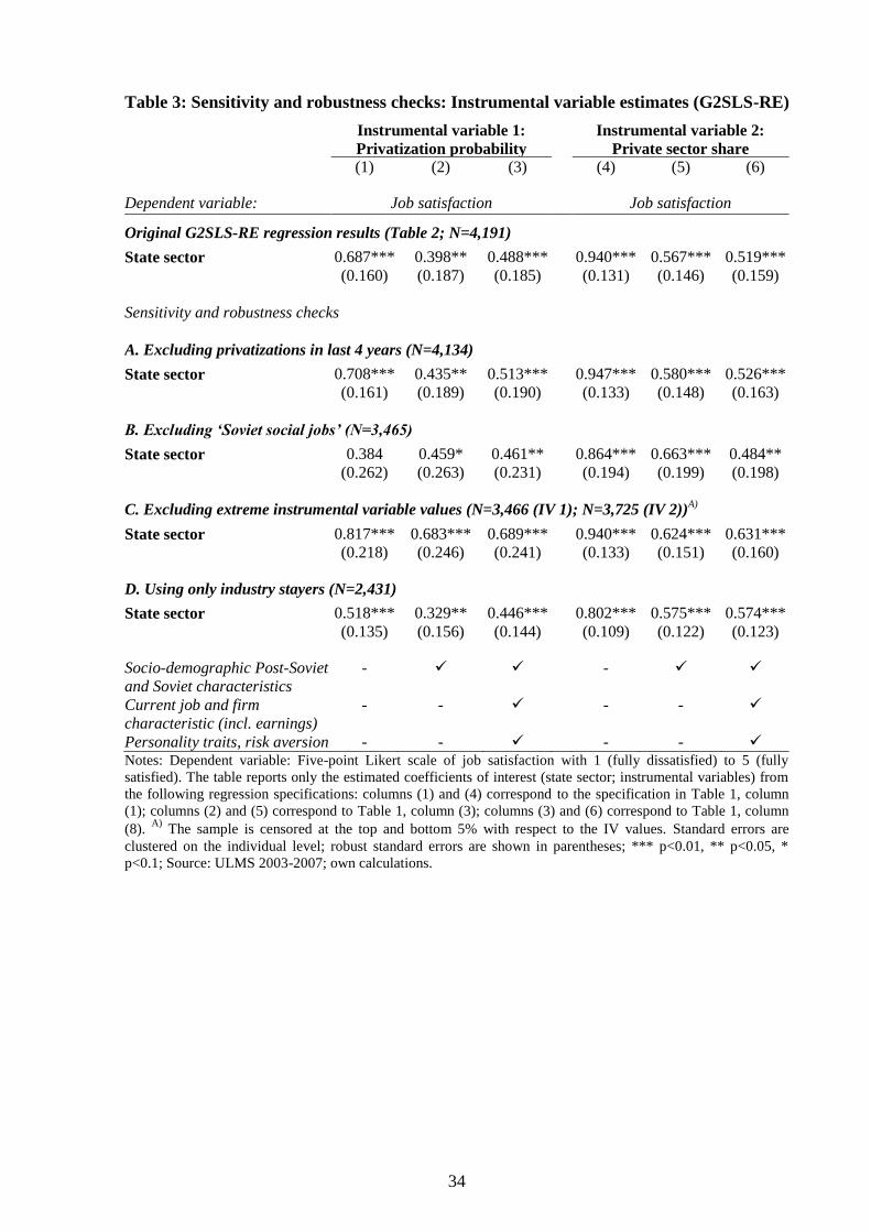
34
Table 3: Sensitivity and robustness checks: Instrumental variable estimates (G2SLS-RE)
Instrumental variable 1:
Privatization probability
Instrumental variable 2:
Private sector share
(1) (2) (3) (4) (5) (6)
Dependent variable: Job satisfaction Job satisfaction
Original G2SLS-RE regression results (Table 2; N=4,191)
State sector 0.687*** 0.398** 0.488*** 0.940*** 0.567*** 0.519***
(0.160) (0.187) (0.185) (0.131) (0.146) (0.159)
Sensitivity and robustness checks
A. Excluding privatizations in last 4 years (N=4,134)
State sector 0.708*** 0.435** 0.513*** 0.947*** 0.580*** 0.526***
(0.161) (0.189) (0.190) (0.133) (0.148) (0.163)
B. Excluding ‘Soviet social jobs’ (N=3,465)
State sector 0.384 0.459* 0.461** 0.864*** 0.663*** 0.484**
(0.262) (0.263) (0.231) (0.194) (0.199) (0.198)
C. Excluding extreme instrumental variable values (N=3,466 (IV 1); N=3,725 (IV 2))A)
State sector 0.817*** 0.683*** 0.689*** 0.940*** 0.624*** 0.631***
(0.218) (0.246) (0.241) (0.133) (0.151) (0.160)
D. Using only industry stayers (N=2,431)
State sector 0.518*** 0.329** 0.446*** 0.802*** 0.575*** 0.574***
(0.135) (0.156) (0.144) (0.109) (0.122) (0.123)
Socio-demographic Post-Soviet
and Soviet characteristics
- -
Current job and firm
characteristic (incl. earnings)
- - - -
Personality traits, risk aversion - - - - Notes: Dependent variable: Five-point Likert scale of job satisfaction with 1 (fully dissatisfied) to 5 (fully
satisfied). The table reports only the estimated coefficients of interest (state sector; instrumental variables) from
the following regression specifications: columns (1) and (4) correspond to the specification in Table 1, column
(1); columns (2) and (5) correspond to Table 1, column (3); columns (3) and (6) correspond to Table 1, column
(8). A)
The sample is censored at the top and bottom 5% with respect to the IV values. Standard errors are
clustered on the individual level; robust standard errors are shown in parentheses; *** p<0.01, ** p<0.05, *
p<0.1; Source: ULMS 2003-2007; own calculations.
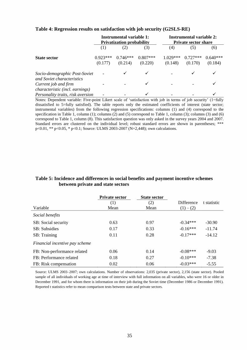
35
Table 4: Regression results on satisfaction with job security (G2SLS-RE)
Instrumental variable 1:
Privatization probability
Instrumental variable 2:
Private sector share
(1) (2) (3) (4) (5) (6)
State sector 0.923*** 0.746*** 0.807*** 1.029*** 0.727*** 0.640***
(0.177) (0.214) (0.220) (0.148) (0.170) (0.184)
Socio-demographic Post-Soviet
and Soviet characteristics
- -
Current job and firm
characteristic (incl. earnings)
- - - -
Personality traits, risk aversion - - - - Notes: Dependent variable: Five-point Likert scale of ‘satisfaction with job in terms of job security’ (1=fully
dissatisfied to 5=fully satisfied). The table reports only the estimated coefficients of interest (state sector;
instrumental variables) from the following regression specifications: columns (1) and (4) correspond to the
specification in Table 1, column (1); columns (2) and (5) correspond to Table 1, column (3); columns (3) and (6)
correspond to Table 1, column (8). This satisfaction question was only asked in the survey years 2004 and 2007.
Standard errors are clustered on the individual level; robust standard errors are shown in parentheses; ***
p<0.01, ** p<0.05, * p<0.1; Source: ULMS 2003-2007 (N=2,448); own calculations.
Table 5: Incidence and differences in social benefits and payment incentive schemes
between private and state sectors
Private sector
State sector
Variable
(1)
Mean
(2)
Mean
Difference
(1) – (2)
t statistic
Social benefits
SB: Social security 0.63 0.97 -0.34*** -30.90
SB: Subsidies 0.17 0.33 -0.16*** -11.74
SB: Training 0.11 0.28 -0.17*** -14.12
Financial incentive pay scheme
FB: Non-performance related 0.06 0.14 -0.08*** -9.03
FB: Performance related 0.18 0.27 -0.10*** -7.38
FB: Risk compensation 0.02 0.06 -0.03*** -5.55
Source: ULMS 2003–2007; own calculations. Number of observations: 2,035 (private sector), 2,156 (state sector). Pooled
sample of all individuals of working age at time of interview with full information on all variables, who were 16 or older in
December 1991, and for whom there is information on their job during the Soviet time (December 1986 or December 1991).
Reported t statistics refer to mean comparison tests between state and private sectors.
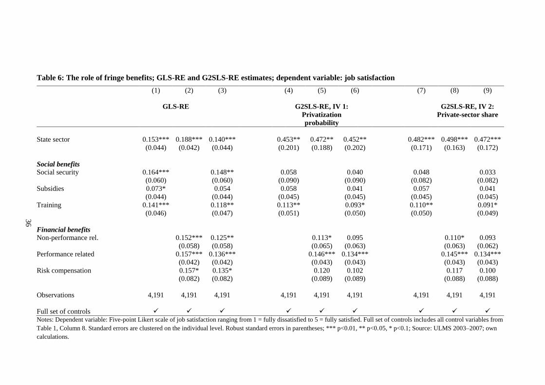
36
Table 6: The role of fringe benefits; GLS-RE and G2SLS-RE estimates; dependent variable: job satisfaction
(1) (2) (3) (4) (5) (6) (7) (8) (9)
GLS-RE G2SLS-RE, IV 1:
Privatization
probability
G2SLS-RE, IV 2:
Private-sector share
State sector 0.153*** 0.188*** 0.140*** 0.453** 0.472** 0.452** 0.482*** 0.498*** 0.472***
(0.044) (0.042) (0.044) (0.201) (0.188) (0.202) (0.171) (0.163) (0.172)
Social benefits
Social security 0.164*** 0.148** 0.058 0.040 0.048 0.033
(0.060) (0.060) (0.090) (0.090) (0.082) (0.082)
Subsidies 0.073* 0.054 0.058 0.041 0.057 0.041
(0.044) (0.044) (0.045) (0.045) (0.045) (0.045)
Training 0.141*** 0.118** 0.113** 0.093* 0.110** 0.091*
(0.046) (0.047) (0.051) (0.050) (0.050) (0.049)
Financial benefits
Non-performance rel. 0.152*** 0.125** 0.113* 0.095 0.110* 0.093
(0.058) (0.058) (0.065) (0.063) (0.063) (0.062)
Performance related 0.157*** 0.136*** 0.146*** 0.134*** 0.145*** 0.134***
(0.042) (0.042) (0.043) (0.043) (0.043) (0.043)
Risk compensation 0.157* 0.135* 0.120 0.102 0.117 0.100
(0.082) (0.082) (0.089) (0.089) (0.088) (0.088)
Observations 4,191 4,191 4,191 4,191 4,191 4,191 4,191 4,191 4,191
Full set of controls Notes: Dependent variable: Five-point Likert scale of job satisfaction ranging from 1 = fully dissatisfied to 5 = fully satisfied. Full set of controls includes all control variables from
Table 1, Column 8. Standard errors are clustered on the individual level. Robust standard errors in parentheses; *** p<0.01, ** p<0.05, * p<0.1; Source: ULMS 2003–2007; own
calculations.
1
(ONLINE) APPENDIX
Job Satisfaction and Self-Selection into the Public or Private Sector:
Evidence from a Natural Experiment
Natalia Danzer
Ifo Institute, University of Munich (LMU),
and IZA Bonn, Germany

2
Appendix A. Additional Tables
Table A 1: Overview on final sample size and labor market composition of original
sample
Cross section 2003
Absolute
numbers
Percentage
Information on final sample size
Total sample 8,537 100.0%
Working A)
3,583 42.0%
out of which
have reached legal minimum working age in 1991 2,943
AND held a job in Dec. 1986 and/or Dec. 1991 2,556
AND have complete information in included variables:
I. Main regression sample with full set of controls 1,491
II. Extended regression sample (excl. variables with many
missings; used for robustness tests)
2,059
Unemployed, ILO 783 9.2%
Out of labor force/student, working age 1,990 23.3%
Out of labor force, pension age 1,827 21.4%
Out of labor force, other 354 4.1% Source: ULMS 2003; own calculations.
A) In official working age (younger than official pension age).
Table A 2: Variable definition
Variable name Variable definition
Satisfaction measures
Job satisfaction Job Satisfaction based on the question: Tell me, please, how satisfied are you
with your current job? Answer option: 1 Fully dissatisfied/ 2 Rather
dissatisfied/ 3 Neither satisfied, nor dissatisfied/ 4 Rather satisfied/ 5 Fully
satisfied (This is the author’s translation of the Russian and Ukrainian
questionnaire. The English version of these answers provided by the survey
institute KIIS is 1—not satisfied at all, 2—less than satisfied, 3—rather
satisfied, 4—satisfied, and 5—fully satisfied, which is misleading.)
Satisfaction with job security Based on the question: Tell me, please, how satisfied are you with your current
job in terms of job security? (Five answer possibilities as in job satisfaction.)
This question was only asked in the survey years 2004 and 2007.
Socio-demographic and household characteristics
Age_35 (omitted cat.)
Age_3640
Age_4145
Age_4650
Age_51ret
Age group dummy variables according to age calculated using birth year,
month, day and interview year, month, day. Last age group: 51 to official
retirement age, which is 55(60) for women(men).
Male = 1, if male; =0 otherwise
Single (omitted cat.) = 1, if marital status is single
Married = 1, if marital status is married (registered or unregistered marriage)
Divorced = 1, if marital status is separated or divorced
Widowed = 1, if marital status is widowed
Primary educationA)
= 1, if person has primary or unfinished secondary education
General secondary education A)
= 1, if person has diploma of high-school or PTU with secondary education
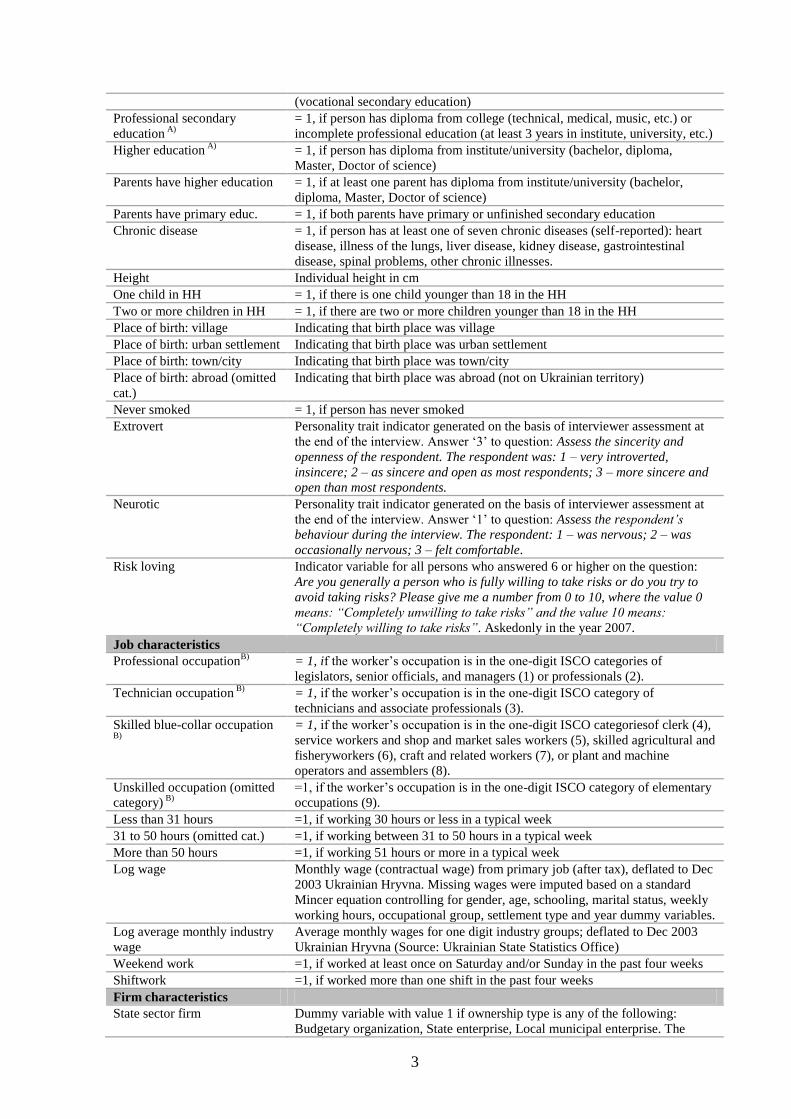
3
(vocational secondary education)
Professional secondary
education A)
= 1, if person has diploma from college (technical, medical, music, etc.) or
incomplete professional education (at least 3 years in institute, university, etc.)
Higher education A)
= 1, if person has diploma from institute/university (bachelor, diploma,
Master, Doctor of science)
Parents have higher education = 1, if at least one parent has diploma from institute/university (bachelor,
diploma, Master, Doctor of science)
Parents have primary educ. = 1, if both parents have primary or unfinished secondary education
Chronic disease = 1, if person has at least one of seven chronic diseases (self-reported): heart
disease, illness of the lungs, liver disease, kidney disease, gastrointestinal
disease, spinal problems, other chronic illnesses.
Height Individual height in cm
One child in HH = 1, if there is one child younger than 18 in the HH
Two or more children in HH = 1, if there are two or more children younger than 18 in the HH
Place of birth: village Indicating that birth place was village
Place of birth: urban settlement Indicating that birth place was urban settlement
Place of birth: town/city Indicating that birth place was town/city
Place of birth: abroad (omitted
cat.)
Indicating that birth place was abroad (not on Ukrainian territory)
Never smoked = 1, if person has never smoked
Extrovert Personality trait indicator generated on the basis of interviewer assessment at
the end of the interview. Answer ‘3’ to question: Assess the sincerity and
openness of the respondent. The respondent was: 1 – very introverted,
insincere; 2 – as sincere and open as most respondents; 3 – more sincere and
open than most respondents.
Neurotic Personality trait indicator generated on the basis of interviewer assessment at
the end of the interview. Answer ‘1’ to question: Assess the respondent’s
behaviour during the interview. The respondent: 1 – was nervous; 2 – was
occasionally nervous; 3 – felt comfortable.
Risk loving Indicator variable for all persons who answered 6 or higher on the question:
Are you generally a person who is fully willing to take risks or do you try to
avoid taking risks? Please give me a number from 0 to 10, where the value 0
means: “Completely unwilling to take risks” and the value 10 means:
“Completely willing to take risks”. Askedonly in the year 2007.
Job characteristics
Professional occupationB)
= 1, if the worker’s occupation is in the one-digit ISCO categories of
legislators, senior officials, and managers (1) or professionals (2).
Technician occupation B)
= 1, if the worker’s occupation is in the one-digit ISCO category of
technicians and associate professionals (3).
Skilled blue-collar occupation
B)
= 1, if the worker’s occupation is in the one-digit ISCO categoriesof clerk (4),
service workers and shop and market sales workers (5), skilled agricultural and
fisheryworkers (6), craft and related workers (7), or plant and machine
operators and assemblers (8).
Unskilled occupation (omitted
category) B)
=1, if the worker’s occupation is in the one-digit ISCO category of elementary
occupations (9).
Less than 31 hours =1, if working 30 hours or less in a typical week
31 to 50 hours (omitted cat.) =1, if working between 31 to 50 hours in a typical week
More than 50 hours =1, if working 51 hours or more in a typical week
Log wage Monthly wage (contractual wage) from primary job (after tax), deflated to Dec
2003 Ukrainian Hryvna. Missing wages were imputed based on a standard
Mincer equation controlling for gender, age, schooling, marital status, weekly
working hours, occupational group, settlement type and year dummy variables.
Log average monthly industry
wage
Average monthly wages for one digit industry groups; deflated to Dec 2003
Ukrainian Hryvna (Source: Ukrainian State Statistics Office)
Weekend work =1, if worked at least once on Saturday and/or Sunday in the past four weeks
Shiftwork =1, if worked more than one shift in the past four weeks
Firm characteristics
State sector firm Dummy variable with value 1 if ownership type is any of the following:
Budgetary organization, State enterprise, Local municipal enterprise. The
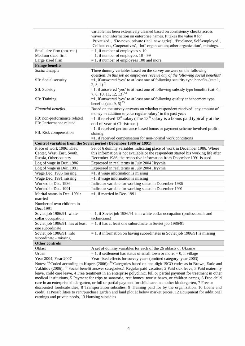
4
variable has been extensively cleaned based on consistency checks across
waves and information on enterprise names. It takes the value 0 for
‘Privatized’, ‘De-novo, private (incl. new agric)’, ‘Freelance, Self-employed’,
‘Collectives, Cooperatives’, ‘Intl' organization; other organization’, missings.
Small size firm (om. cat.)
Medium sized firm
Large sized firm
= 1, if number of employees < 10
= 1, if number of employees 10 - 99
= 1, if number of employees 100 and more
Fringe benefits
Social benefits
SB: Social security
SB: Subsidy
SB: Training
Three dummy variables based on the survey answers on the following
question: In this job do employees receive any of the following social benefits?
=1, if answered ‘yes’ to at least one of following security type benefits (cat: 1,
2, 3, 4) C)
=1, if answered ‘yes’ to at least one of following subsidy type benefits (cat: 6,
7, 8, 10, 11, 12, 13) C)
=1, if answered ‘yes’ to at least one of following quality enhancement type
benefits (cat: 9, 5) C)
Financial benefits
FB: non-performance related
FB: Performance related
FB: Risk compensation
Based on the survey answers on whether respondent received ‘any amount of
money in addition to your regular salary’ in the past year:
=1, if received 13th
salary (The 13th salary is a bonus paid typically at the
end of year at Christmas.) =1, if received performance-based bonus or payment scheme involved profit-
sharing
=1, if received compensation for non-normal work conditions
Control variables from the Soviet period (December 1986 or 1991)
Place of work 1986: Kiev,
Center, West, East, South,
Russia, Other country
Set of 6 dummy variables indicating place of work in December 1986. Where
this information is not available or the respondent started his working life after
December 1986, the respective information from December 1991 is used.
Log of wage in Dec. 1986 Expressed in real terms in July 2004 Hryvnia
Log of wage in Dec. 1991 Expressed in real terms in July 2004 Hryvnia
Wage Dec. 1986 missing =1, if wage information is missing
Wage Dec. 1991 missing =1, if wage information is missing
Worked in Dec. 1986 Indicator variable for working status in December 1986
Worked in Dec. 1991 Indicator variable for working status in December 1991
Marital status in Dec. 1991:
married
=1, if married in Dec. 1991
Number of own children in
Dec. 1991
Soviet job 1986/91: white
collar occupation
= 1, if Soviet job 1986/91 is in white collar occupation (professionals and
technicians)
Soviet job 1986/91: has at least
one subordinate
= 1, if has at least one subordinate in Soviet job 1986/91
Soviet job 1986/91: info
subordinate - missing
= 1, if information on having subordinates in Soviet job 1986/91 is missing
Other controls
Oblast A set of dummy variables for each of the 26 oblasts of Ukraine
Urban = 1, if settlement has status of small town or more, = 0, if village
Year 2004, Year 2007 Year fixed effects for survey years (omitted category: year 2003)
Notes: A)
Coded according to Kupets (2006); B)
Categories based on one-digit ISCO codes as in Brown, Earle and
Vakhitov (2006); C)
Social benefit answer categories:1 Regular paid vacation, 2 Paid sick leave, 3 Paid maternity
leave, child care leave, 4 Free treatment in an enterprise polyclinic, full or partial payment for treatment in other
medical institutions, 5 Payment for trips to sanatoria, rest homes, tourist bases, or children camps, 6 Free child
care in an enterprise kindergarten, or full or partial payment for child care in another kindergarten, 7 Free or
discounted food/subsidies, 8 Transportation subsidies, 9 Training paid for by the organization, 10 Loans and
credit, 11Possibilities to rent/purchase garden and land plot at below market prices, 12 Equipment for additional
earnings and private needs, 13 Housing subsidies
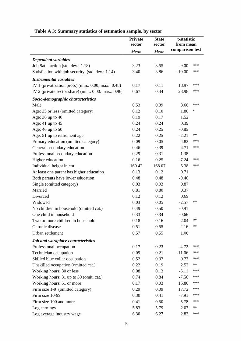
5
Table A 3: Summary statistics of estimation sample, by sector
Private
sector
State
sector
t-statistic
from mean
Mean Mean
comparison test
Dependent variables
Job Satisfaction (std. dev.: 1.18) 3.23 3.55 -9.00 ***
Satisfaction with job security (std. dev.: 1.14) 3.40 3.86 -10.00 ***
Instrumental variables
IV 1 (privatization prob.) (min.: 0.00; max.: 0.48) 0.17 0.11 18.97 ***
IV 2 (private sector share) (min.: 0.00: max.: 0.96) 0.67 0.44 23.98 ***
Socio-demographic characteristics
Male 0.53 0.39 8.68 ***
Age: 35 or less (omitted category) 0.12 0.10 1.80 *
Age: 36 up to 40 0.19 0.17 1.52
Age: 41 up to 45 0.24 0.24 0.39
Age: 46 up to 50 0.24 0.25 -0.85
Age: 51 up to retirement age 0.22 0.25 -2.21 **
Primary education (omitted category) 0.09 0.05 4.82 ***
General secondary education 0.46 0.39 4.71 ***
Professional secondary education 0.29 0.31 -1.38
Higher education 0.16 0.25 -7.24 ***
Individual height in cm. 169.42 168.07 5.38 ***
At least one parent has higher education 0.13 0.12 0.71
Both parents have lower education 0.48 0.48 -0.46
Single (omitted category) 0.03 0.03 0.87
Married 0.81 0.80 0.37
Divorced 0.12 0.12 0.69
Widowed 0.03 0.05 -2.57 **
No children in household (omitted cat.) 0.49 0.50 -0.91
One child in household 0.33 0.34 -0.66
Two or more children in household 0.18 0.16 2.04 **
Chronic disease 0.51 0.55 -2.16 **
Urban settlement 0.57 0.55 1.06
Job and workplace characteristics
Professional occupation 0.17 0.23 -4.72 ***
Technician occupation 0.09 0.21 -11.06 ***
Skilled blue collar occupation 0.52 0.37 9.77 ***
Unskilled occupation (omitted cat.) 0.22 0.19 2.52 **
Working hours: 30 or less 0.08 0.13 -5.11 ***
Working hours: 31 up to 50 (omit. cat.) 0.74 0.84 -7.56 ***
Working hours: 51 or more 0.17 0.03 15.80 ***
Firm size 1-9 (omitted category) 0.29 0.09 17.72 ***
Firm size 10-99 0.30 0.41 -7.91 ***
Firm size 100 and more 0.41 0.50 -5.78 ***
Log earnings 5.83 5.79 2.07 **
Log average industry wage 6.30 6.27 2.83 ***
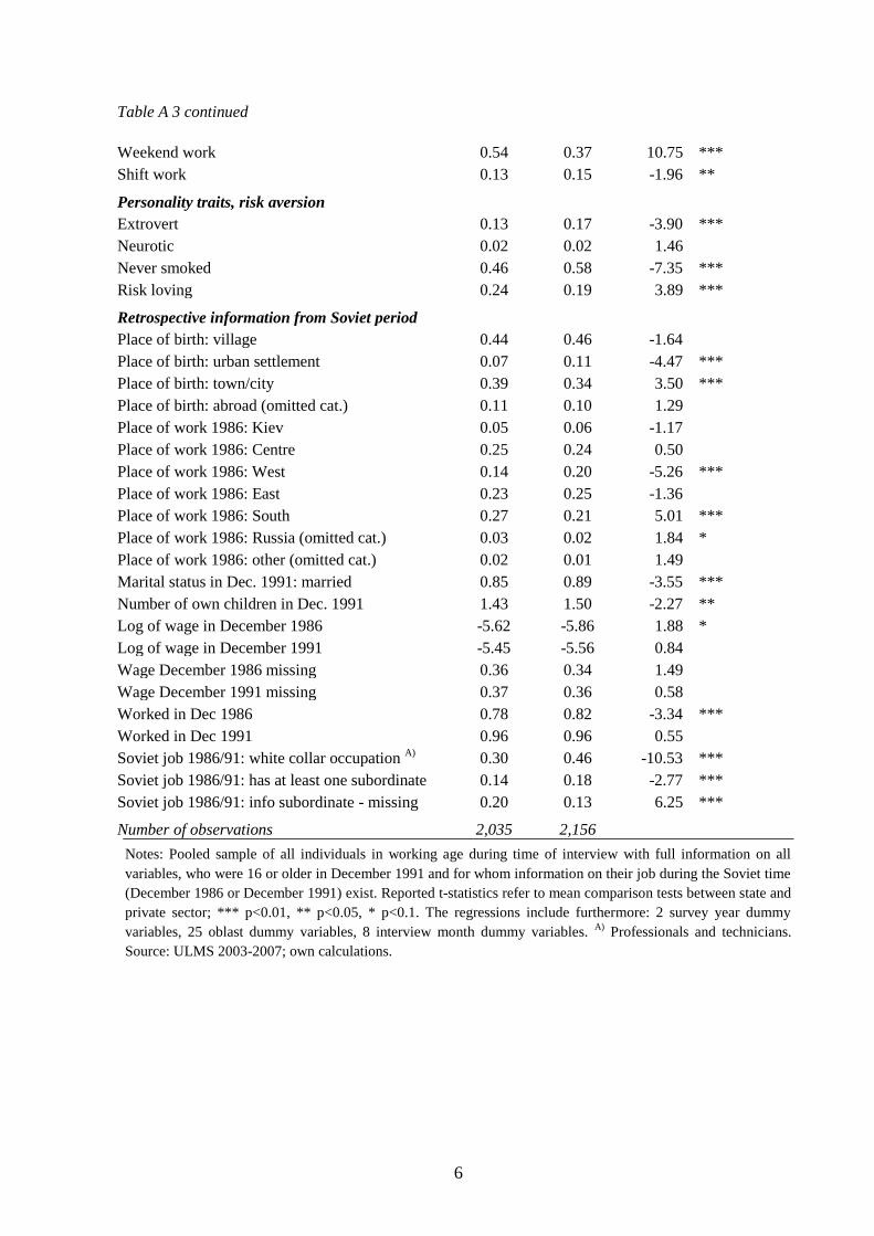
6
Table A 3 continued
Weekend work 0.54 0.37 10.75 ***
Shift work 0.13 0.15 -1.96 **
Personality traits, risk aversion
Extrovert 0.13 0.17 -3.90 ***
Neurotic 0.02 0.02 1.46
Never smoked 0.46 0.58 -7.35 ***
Risk loving 0.24 0.19 3.89 ***
Retrospective information from Soviet period
Place of birth: village 0.44 0.46 -1.64
Place of birth: urban settlement 0.07 0.11 -4.47 ***
Place of birth: town/city 0.39 0.34 3.50 ***
Place of birth: abroad (omitted cat.) 0.11 0.10 1.29
Place of work 1986: Kiev 0.05 0.06 -1.17
Place of work 1986: Centre 0.25 0.24 0.50
Place of work 1986: West 0.14 0.20 -5.26 ***
Place of work 1986: East 0.23 0.25 -1.36
Place of work 1986: South 0.27 0.21 5.01 ***
Place of work 1986: Russia (omitted cat.) 0.03 0.02 1.84 *
Place of work 1986: other (omitted cat.) 0.02 0.01 1.49
Marital status in Dec. 1991: married 0.85 0.89 -3.55 ***
Number of own children in Dec. 1991 1.43 1.50 -2.27 **
Log of wage in December 1986 -5.62 -5.86 1.88 *
Log of wage in December 1991 -5.45 -5.56 0.84
Wage December 1986 missing 0.36 0.34 1.49
Wage December 1991 missing 0.37 0.36 0.58
Worked in Dec 1986 0.78 0.82 -3.34 ***
Worked in Dec 1991 0.96 0.96 0.55
Soviet job 1986/91: white collar occupation A)
0.30 0.46 -10.53 ***
Soviet job 1986/91: has at least one subordinate 0.14 0.18 -2.77 ***
Soviet job 1986/91: info subordinate - missing 0.20 0.13 6.25 ***
Number of observations 2,035 2,156
Notes: Pooled sample of all individuals in working age during time of interview with full information on all
variables, who were 16 or older in December 1991 and for whom information on their job during the Soviet time
(December 1986 or December 1991) exist. Reported t-statistics refer to mean comparison tests between state and
private sector; *** p<0.01, ** p<0.05, * p<0.1. The regressions include furthermore: 2 survey year dummy
variables, 25 oblast dummy variables, 8 interview month dummy variables. A)
Professionals and technicians.
Source: ULMS 2003-2007; own calculations.
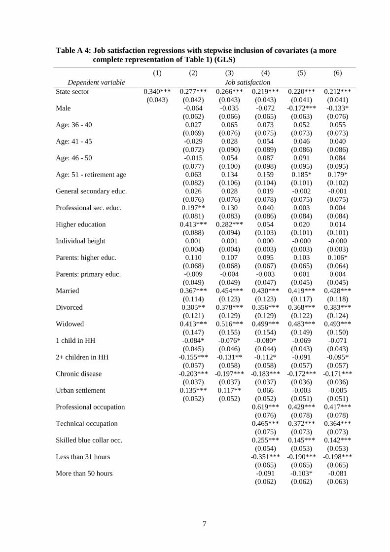
7
Table A 4: Job satisfaction regressions with stepwise inclusion of covariates (a more
complete representation of Table 1) (GLS)
(1) (2) (3) (4) (5) (6)
Dependent variable Job satisfaction
State sector 0.340*** 0.277*** 0.266*** 0.219*** 0.220*** 0.212***
(0.043) (0.042) (0.043) (0.043) (0.041) (0.041)
Male -0.064 -0.035 -0.072 -0.172*** -0.133*
(0.062) (0.066) (0.065) (0.063) (0.076)
Age: 36 - 40 0.027 0.065 0.073 0.052 0.055
(0.069) (0.076) (0.075) (0.073) (0.073)
Age: 41 - 45 -0.029 0.028 0.054 0.046 0.040
(0.072) (0.090) (0.089) (0.086) (0.086)
Age: 46 - 50 -0.015 0.054 0.087 0.091 0.084
(0.077) (0.100) (0.098) (0.095) (0.095)
Age: 51 - retirement age 0.063 0.134 0.159 0.185* 0.179*
(0.082) (0.106) (0.104) (0.101) (0.102)
General secondary educ. 0.026 0.028 0.019 -0.002 -0.001
(0.076) (0.076) (0.078) (0.075) (0.075)
Professional sec. educ. 0.197** 0.130 0.040 0.003 0.004
(0.081) (0.083) (0.086) (0.084) (0.084)
Higher education 0.413*** 0.282*** 0.054 0.020 0.014
(0.088) (0.094) (0.103) (0.101) (0.101)
Individual height 0.001 0.001 0.000 -0.000 -0.000
(0.004) (0.004) (0.003) (0.003) (0.003)
Parents: higher educ. 0.110 0.107 0.095 0.103 0.106*
(0.068) (0.068) (0.067) (0.065) (0.064)
Parents: primary educ. -0.009 -0.004 -0.003 0.001 0.004
(0.049) (0.049) (0.047) (0.045) (0.045)
Married 0.367*** 0.454*** 0.430*** 0.419*** 0.428***
(0.114) (0.123) (0.123) (0.117) (0.118)
Divorced 0.305** 0.378*** 0.356*** 0.368*** 0.383***
(0.121) (0.129) (0.129) (0.122) (0.124)
Widowed 0.413*** 0.516*** 0.499*** 0.483*** 0.493***
(0.147) (0.155) (0.154) (0.149) (0.150)
1 child in HH -0.084* -0.076* -0.080* -0.069 -0.071
(0.045) (0.046) (0.044) (0.043) (0.043)
2+ children in HH -0.155*** -0.131** -0.112* -0.091 -0.095*
(0.057) (0.058) (0.058) (0.057) (0.057)
Chronic disease -0.203*** -0.197*** -0.183*** -0.172*** -0.171***
(0.037) (0.037) (0.037) (0.036) (0.036)
Urban settlement 0.135*** 0.117** 0.066 -0.003 -0.005
(0.052) (0.052) (0.052) (0.051) (0.051)
Professional occupation 0.619*** 0.429*** 0.417***
(0.076) (0.078) (0.078)
Technical occupation 0.465*** 0.372*** 0.364***
(0.075) (0.073) (0.073)
Skilled blue collar occ. 0.255*** 0.145*** 0.142***
(0.054) (0.053) (0.053)
Less than 31 hours -0.351*** -0.190*** -0.198***
(0.065) (0.065) (0.065)
More than 50 hours -0.091 -0.103* -0.081
(0.062) (0.062) (0.063)
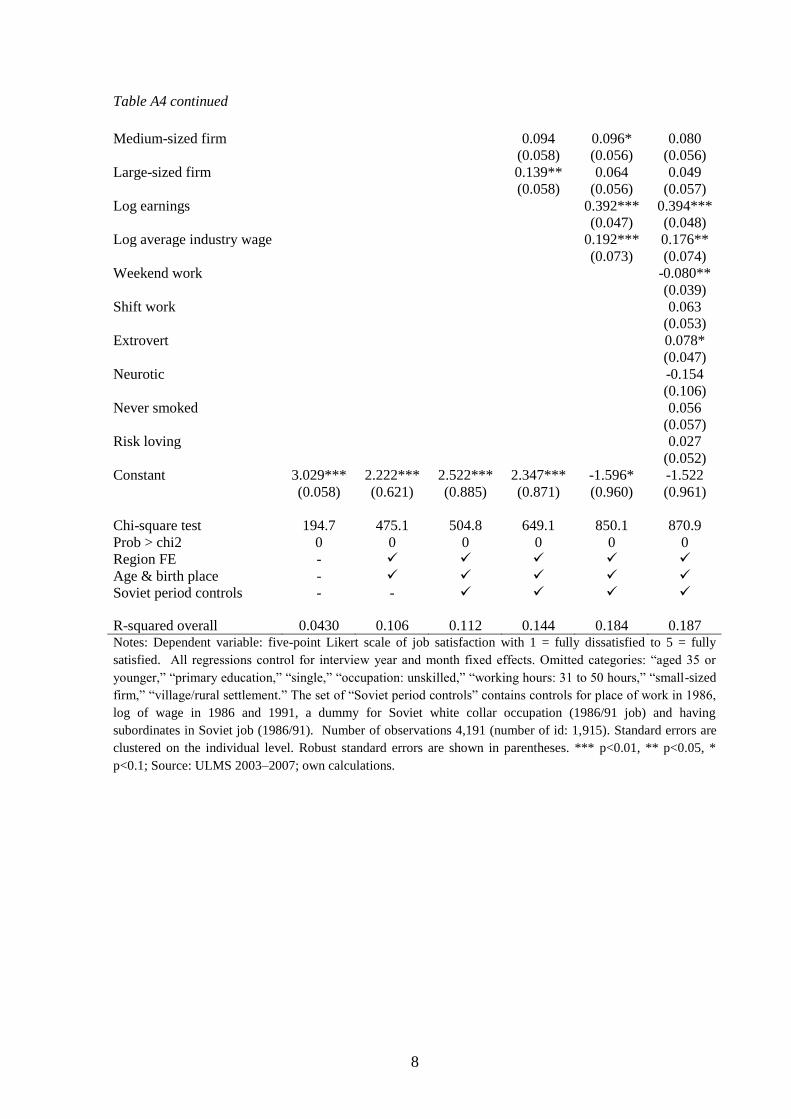
8
Table A4 continued
Medium-sized firm 0.094 0.096* 0.080
(0.058) (0.056) (0.056)
Large-sized firm 0.139** 0.064 0.049
(0.058) (0.056) (0.057)
Log earnings 0.392*** 0.394***
(0.047) (0.048)
Log average industry wage 0.192*** 0.176**
(0.073) (0.074)
Weekend work -0.080**
(0.039)
Shift work 0.063
(0.053)
Extrovert 0.078*
(0.047)
Neurotic -0.154
(0.106)
Never smoked 0.056
(0.057)
Risk loving 0.027
(0.052)
Constant 3.029*** 2.222*** 2.522*** 2.347*** -1.596* -1.522
(0.058) (0.621) (0.885) (0.871) (0.960) (0.961)
Chi-square test 194.7 475.1 504.8 649.1 850.1 870.9
Prob > chi2 0 0 0 0 0 0
Region FE -
Age & birth place -
Soviet period controls - -
R-squared overall 0.0430 0.106 0.112 0.144 0.184 0.187 Notes: Dependent variable: five-point Likert scale of job satisfaction with 1 = fully dissatisfied to 5 = fully
satisfied. All regressions control for interview year and month fixed effects. Omitted categories: “aged 35 or
younger,” “primary education,” “single,” “occupation: unskilled,” “working hours: 31 to 50 hours,” “small-sized
firm,” “village/rural settlement.” The set of “Soviet period controls” contains controls for place of work in 1986,
log of wage in 1986 and 1991, a dummy for Soviet white collar occupation (1986/91 job) and having
subordinates in Soviet job (1986/91). Number of observations 4,191 (number of id: 1,915). Standard errors are
clustered on the individual level. Robust standard errors are shown in parentheses. *** p<0.01, ** p<0.05, *
p<0.1; Source: ULMS 2003–2007; own calculations.
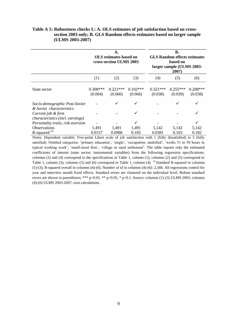
9
Table A 5: Robustness checks I.: A. OLS estimates of job satisfaction based on cross-
section 2003 only; B. GLS Random effects estimates based on larger sample
(ULMS 2003-2007)
A.
OLS estimates based on
cross-section ULMS 2003
B.
GLS Random effects estimates
based on
larger sample (ULMS 2003-
2007)
(1) (2) (3) (4) (5) (6)
State sector 0.308*** 0.221*** 0.192*** 0.321*** 0.255*** 0.208***
(0.064) (0.066) (0.066) (0.038) (0.039) (0.038)
Socio-demographic Post-Soviet
& Soviet characteristics
- -
Current job & firm
characteristics (incl. earnings)
- - - -
Personality traits, risk aversion - - - -
Observations 1,491 1,491 1,491 5,142 5,142 5,142
R-squared A)
0.0157 0.0986 0.185 0.0381 0.103 0.182 Notes: Dependent variable: Five-point Likert scale of job satisfaction with 1 (fully dissatisfied) to 5 (fully
satisfied). Omitted categories: ‘primary education’, ‘single’, ‘occupation: unskilled’, ‘works 31 to 50 hours in
typical working week’, ‘small-sized firm’, ‘village or rural settlement’. The table reports only the estimated
coefficients of interest (state sector; instrumental variables) from the following regression specifications:
columns (1) and (4) correspond to the specifications in Table 1, column (1); columns (2) and (5) correspond to
Table 1, column (3); columns (3) and (6) correspond to Table 1, column (4). A)
Standard R-squared in columns
(1)-(3); R-squared overall in columns (4)-(6). Number of id in columns (4)-(6): 2,566. All regressions control for
year and interview month fixed effects. Standard errors are clustered on the individual level. Robust standard
errors are shown in parentheses; *** p<0.01, ** p<0.05, * p<0.1. Source: columns (1)-(3) ULMS 2003, columns
(4)-(6) ULMS 2003-2007; own calculations.
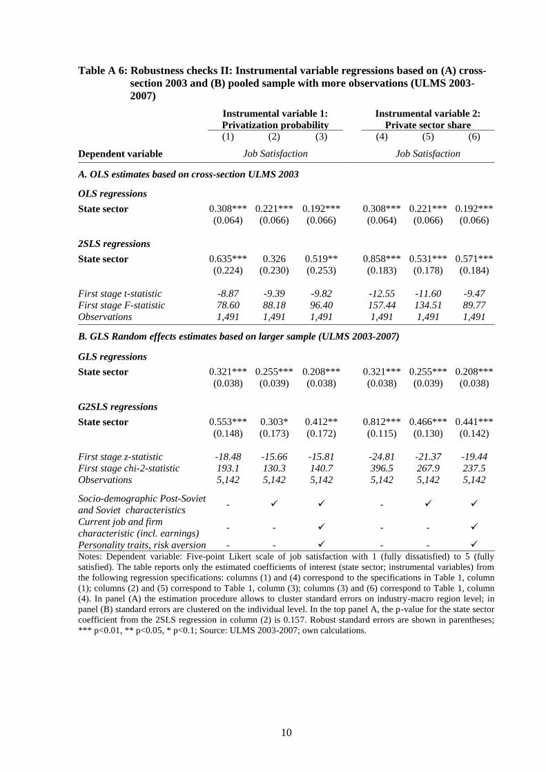
10
Table A 6: Robustness checks II: Instrumental variable regressions based on (A) cross-
section 2003 and (B) pooled sample with more observations (ULMS 2003-
2007)
Instrumental variable 1:
Privatization probability
Instrumental variable 2:
Private sector share
(1) (2) (3) (4) (5) (6)
Dependent variable Job Satisfaction Job Satisfaction
A. OLS estimates based on cross-section ULMS 2003
OLS regressions
State sector 0.308*** 0.221*** 0.192*** 0.308*** 0.221*** 0.192***
(0.064) (0.066) (0.066) (0.064) (0.066) (0.066)
2SLS regressions
State sector 0.635*** 0.326 0.519** 0.858*** 0.531*** 0.571***
(0.224) (0.230) (0.253) (0.183) (0.178) (0.184)
First stage t-statistic -8.87 -9.39 -9.82 -12.55 -11.60 -9.47
First stage F-statistic 78.60 88.18 96.40 157.44 134.51 89.77
Observations 1,491 1,491 1,491 1,491 1,491 1,491
B. GLS Random effects estimates based on larger sample (ULMS 2003-2007)
GLS regressions
State sector 0.321*** 0.255*** 0.208*** 0.321*** 0.255*** 0.208***
(0.038) (0.039) (0.038) (0.038) (0.039) (0.038)
G2SLS regressions
State sector 0.553*** 0.303* 0.412** 0.812*** 0.466*** 0.441***
(0.148) (0.173) (0.172) (0.115) (0.130) (0.142)
First stage z-statistic -18.48 -15.66 -15.81 -24.81 -21.37 -19.44
First stage chi-2-statistic 193.1 130.3 140.7 396.5 267.9 237.5
Observations 5,142 5,142 5,142 5,142 5,142 5,142
Socio-demographic Post-Soviet
and Soviet characteristics - -
Current job and firm
characteristic (incl. earnings) - - - -
Personality traits, risk aversion - - - - Notes: Dependent variable: Five-point Likert scale of job satisfaction with 1 (fully dissatisfied) to 5 (fully
satisfied). The table reports only the estimated coefficients of interest (state sector; instrumental variables) from
the following regression specifications: columns (1) and (4) correspond to the specifications in Table 1, column
(1); columns (2) and (5) correspond to Table 1, column (3); columns (3) and (6) correspond to Table 1, column
(4). In panel (A) the estimation procedure allows to cluster standard errors on industry-macro region level; in
panel (B) standard errors are clustered on the individual level. In the top panel A, the p-value for the state sector
coefficient from the 2SLS regression in column (2) is 0.157. Robust standard errors are shown in parentheses;
*** p<0.01, ** p<0.05, * p<0.1; Source: ULMS 2003-2007; own calculations.

11
Appendix B. Construction of instrumental variables
First Instrumental Variable: Share of Employees experiencing privatization in 27
industries
The first instrumental variable reflects the probability of experiencing subsequent
privatization of one’s Soviet workplace in a specific industry sector. The calculation of the
instrumental variable exploits the retrospective work histories of the ULMS 2003. It is based
on the sample of individuals starting their jobs during the Soviet period and who stayed in
these jobs at least until January 1993, i.e. until the start of the mass privatization process
(creating a sample of 4,451 individual ‘transition jobs’). The calculation of industry specific
privatization probabilities involves two steps: (1) First, a binary indicator is generated for
each ‘transition job’ taking the value ‘1’ if the workplace was privatized during the tenure of
the job and if most of the shares of the enterprise/organization were owned by private entities
after the privatization, and ‘0’ otherwise. (2) Second, these binary privatization indicators are
used to calculate the share of privatized jobs within 27 different industry sectors (see Table B
1 for the calculated privatization probabilities and the respective cell sizes). These industry
specific privatization probabilities are assigned to workers according to the industry in which
they used to work in December 1986. For the subsample of workers who did not work in
December 1986, but started to work before December 1991, the industry specific privatization
probability is assigned according to the industry of their job held in December 1991. Note,
that there are two aspects that potentially reduce the exactness of this instrumental variable in
reflecting the true industry specific privatization probability. First, the ULMS survey was
originally designed to be representative of the Ukrainian population aged 15 to 72 in 2003 and
not in 1986/1991. This implies that the true privatization probabilities might differ to the
extent that the distribution of workers across industries based on the retrospective information
of the sample 2003 differs from the actual distribution (if, for instance, mortality rates or
migration vary across industries). Second, the construction of the instrumental variable is
based only on those jobs that started during the Soviet period and thus neglects all possible
privatization experiences after a job change in the Post-Soviet period. However, this will only
bias the estimates if the workers propensity to leave a ‘still state-owned’ enterprise before its
privatization differs systematically across sectors.
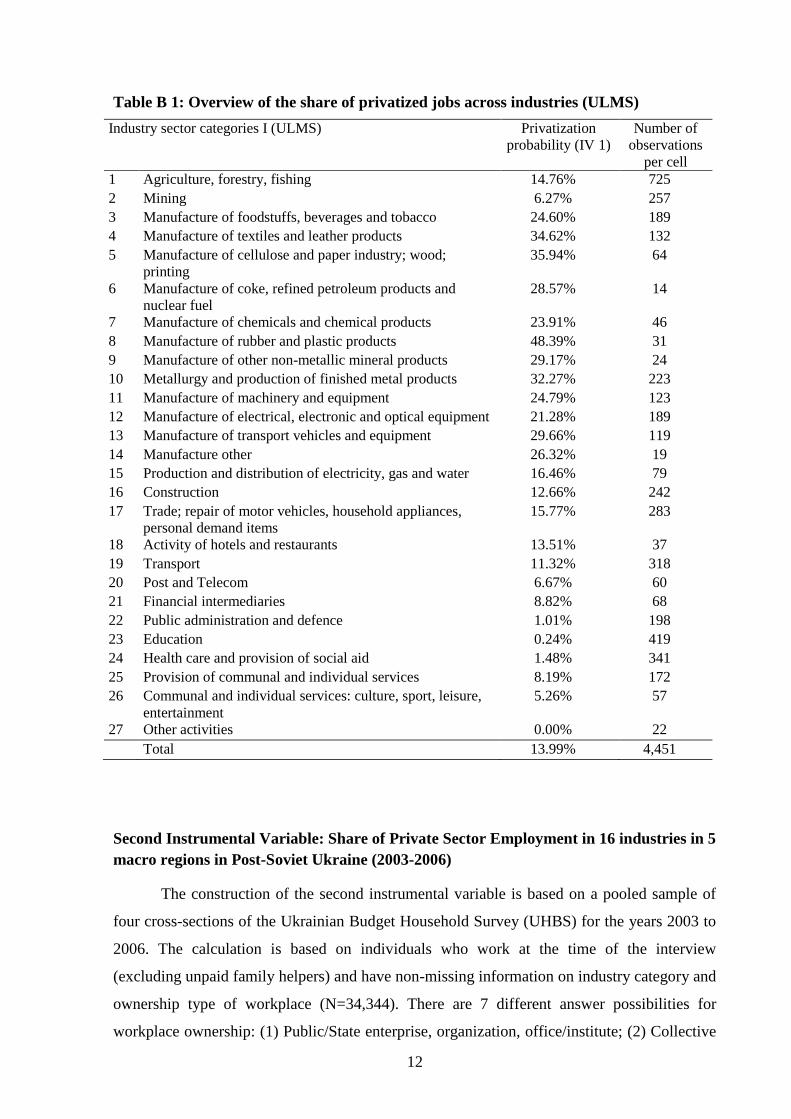
12
Table B 1: Overview of the share of privatized jobs across industries (ULMS)
Industry sector categories I (ULMS) Privatization
probability (IV 1)
Number of
observations
per cell
1 Agriculture, forestry, fishing 14.76% 725
2 Mining 6.27% 257
3 Manufacture of foodstuffs, beverages and tobacco 24.60% 189
4 Manufacture of textiles and leather products 34.62% 132
5 Manufacture of cellulose and paper industry; wood;
printing
35.94% 64
6 Manufacture of coke, refined petroleum products and
nuclear fuel
28.57% 14
7 Manufacture of chemicals and chemical products 23.91% 46
8 Manufacture of rubber and plastic products 48.39% 31
9 Manufacture of other non-metallic mineral products 29.17% 24
10 Metallurgy and production of finished metal products 32.27% 223
11 Manufacture of machinery and equipment 24.79% 123
12 Manufacture of electrical, electronic and optical equipment 21.28% 189
13 Manufacture of transport vehicles and equipment 29.66% 119
14 Manufacture other 26.32% 19
15 Production and distribution of electricity, gas and water 16.46% 79
16 Construction 12.66% 242
17 Trade; repair of motor vehicles, household appliances,
personal demand items
15.77% 283
18 Activity of hotels and restaurants 13.51% 37
19 Transport 11.32% 318
20 Post and Telecom 6.67% 60
21 Financial intermediaries 8.82% 68
22 Public administration and defence 1.01% 198
23 Education 0.24% 419
24 Health care and provision of social aid 1.48% 341
25 Provision of communal and individual services 8.19% 172
26 Communal and individual services: culture, sport, leisure,
entertainment
5.26% 57
27 Other activities 0.00% 22
Total 13.99% 4,451
Second Instrumental Variable: Share of Private Sector Employment in 16 industries in 5
macro regions in Post-Soviet Ukraine (2003-2006)
The construction of the second instrumental variable is based on a pooled sample of
four cross-sections of the Ukrainian Budget Household Survey (UHBS) for the years 2003 to
2006. The calculation is based on individuals who work at the time of the interview
(excluding unpaid family helpers) and have non-missing information on industry category and
ownership type of workplace (N=34,344). There are 7 different answer possibilities for
workplace ownership: (1) Public/State enterprise, organization, office/institute; (2) Collective
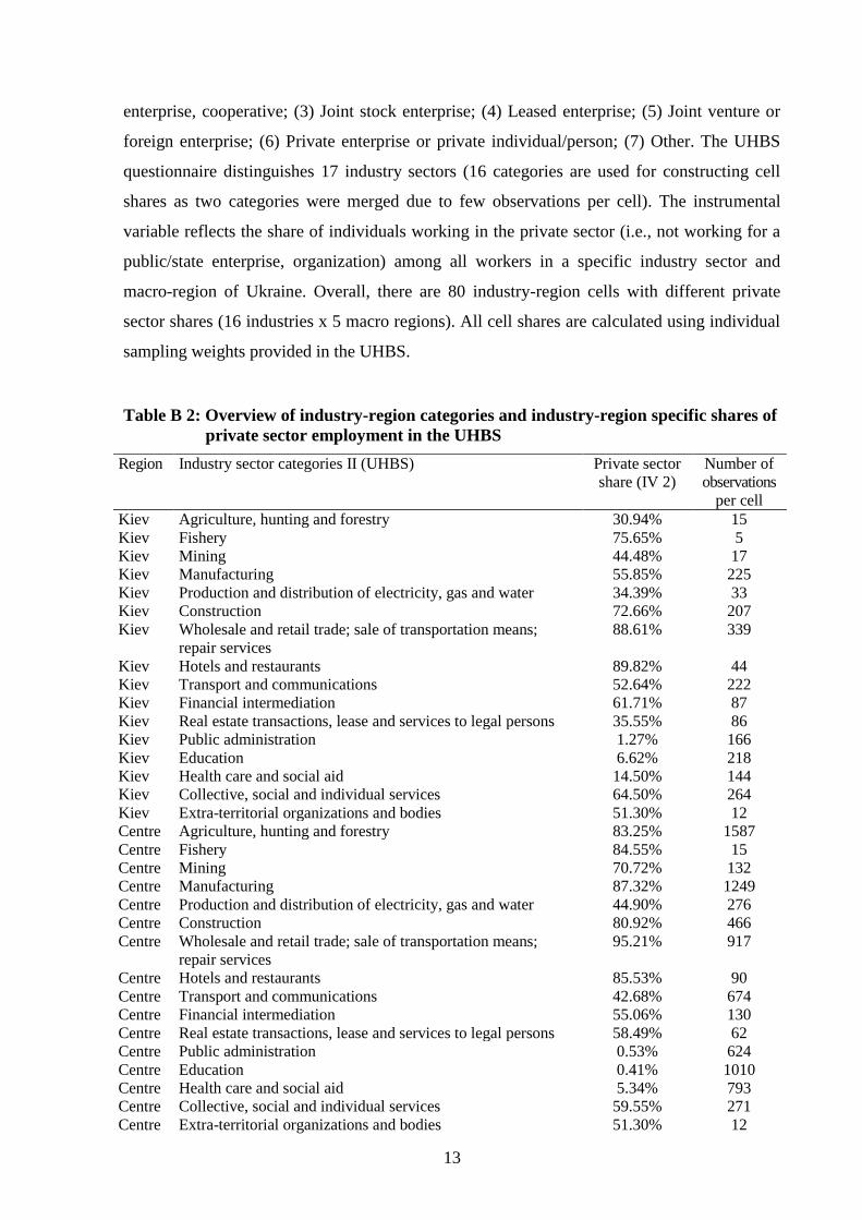
13
enterprise, cooperative; (3) Joint stock enterprise; (4) Leased enterprise; (5) Joint venture or
foreign enterprise; (6) Private enterprise or private individual/person; (7) Other. The UHBS
questionnaire distinguishes 17 industry sectors (16 categories are used for constructing cell
shares as two categories were merged due to few observations per cell). The instrumental
variable reflects the share of individuals working in the private sector (i.e., not working for a
public/state enterprise, organization) among all workers in a specific industry sector and
macro-region of Ukraine. Overall, there are 80 industry-region cells with different private
sector shares (16 industries x 5 macro regions). All cell shares are calculated using individual
sampling weights provided in the UHBS.
Table B 2: Overview of industry-region categories and industry-region specific shares of
private sector employment in the UHBS
Region Industry sector categories II (UHBS) Private sector
share (IV 2)
Number of
observations
per cell
Kiev Agriculture, hunting and forestry 30.94% 15
Kiev Fishery 75.65% 5
Kiev Mining 44.48% 17
Kiev Manufacturing 55.85% 225
Kiev Production and distribution of electricity, gas and water 34.39% 33
Kiev Construction 72.66% 207
Kiev Wholesale and retail trade; sale of transportation means;
repair services
88.61% 339
Kiev Hotels and restaurants 89.82% 44
Kiev Transport and communications 52.64% 222
Kiev Financial intermediation 61.71% 87
Kiev Real estate transactions, lease and services to legal persons 35.55% 86
Kiev Public administration 1.27% 166
Kiev Education 6.62% 218
Kiev Health care and social aid 14.50% 144
Kiev Collective, social and individual services 64.50% 264
Kiev Extra-territorial organizations and bodies 51.30% 12
Centre Agriculture, hunting and forestry 83.25% 1587
Centre Fishery 84.55% 15
Centre Mining 70.72% 132
Centre Manufacturing 87.32% 1249
Centre Production and distribution of electricity, gas and water 44.90% 276
Centre Construction 80.92% 466
Centre Wholesale and retail trade; sale of transportation means;
repair services
95.21% 917
Centre Hotels and restaurants 85.53% 90
Centre Transport and communications 42.68% 674
Centre Financial intermediation 55.06% 130
Centre Real estate transactions, lease and services to legal persons 58.49% 62
Centre Public administration 0.53% 624
Centre Education 0.41% 1010
Centre Health care and social aid 5.34% 793
Centre Collective, social and individual services 59.55% 271
Centre Extra-territorial organizations and bodies 51.30% 12
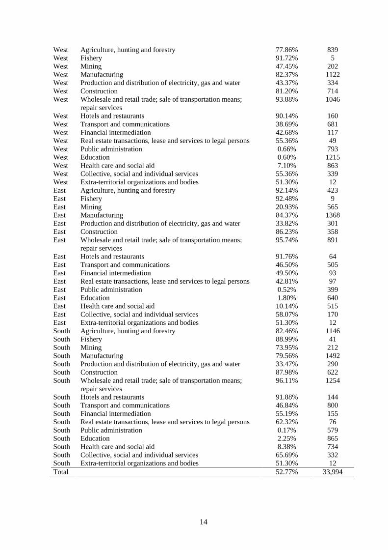
14
West Agriculture, hunting and forestry 77.86% 839
West Fishery 91.72% 5
West Mining 47.45% 202
West Manufacturing 82.37% 1122
West Production and distribution of electricity, gas and water 43.37% 334
West Construction 81.20% 714
West Wholesale and retail trade; sale of transportation means;
repair services
93.88% 1046
West Hotels and restaurants 90.14% 160
West Transport and communications 38.69% 681
West Financial intermediation 42.68% 117
West Real estate transactions, lease and services to legal persons 55.36% 49
West Public administration 0.66% 793
West Education 0.60% 1215
West Health care and social aid 7.10% 863
West Collective, social and individual services 55.36% 339
West Extra-territorial organizations and bodies 51.30% 12
East Agriculture, hunting and forestry 92.14% 423
East Fishery 92.48% 9
East Mining 20.93% 565
East Manufacturing 84.37% 1368
East Production and distribution of electricity, gas and water 33.82% 301
East Construction 86.23% 358
East Wholesale and retail trade; sale of transportation means;
repair services
95.74% 891
East Hotels and restaurants 91.76% 64
East Transport and communications 46.50% 505
East Financial intermediation 49.50% 93
East Real estate transactions, lease and services to legal persons 42.81% 97
East Public administration 0.52% 399
East Education 1.80% 640
East Health care and social aid 10.14% 515
East Collective, social and individual services 58.07% 170
East Extra-territorial organizations and bodies 51.30% 12
South Agriculture, hunting and forestry 82.46% 1146
South Fishery 88.99% 41
South Mining 73.95% 212
South Manufacturing 79.56% 1492
South Production and distribution of electricity, gas and water 33.47% 290
South Construction 87.98% 622
South Wholesale and retail trade; sale of transportation means;
repair services
96.11% 1254
South Hotels and restaurants 91.88% 144
South Transport and communications 46.84% 800
South Financial intermediation 55.19% 155
South Real estate transactions, lease and services to legal persons 62.32% 76
South Public administration 0.17% 579
South Education 2.25% 865
South Health care and social aid 8.38% 734
South Collective, social and individual services 65.69% 332
South Extra-territorial organizations and bodies 51.30% 12
Total 52.77% 33,994
Recommended