Dipartimento di Scienze Statistiche Sezione di Statistica Economica ed Econometria
S. Delle Chiaie, B. Maggi
Italian Government debt liquidity, is it of value?
DSS Empirical Economics and EconometricsWorking Papers Series
DSS-E3 WP 2014/3

Dipartimento di Scienze StatisticheSezione di Statistica Economica ed Econometria
“Sapienza” Università di RomaP.le A. Moro 5 – 00185 Roma - Italia
http://www.dss.uniroma1.it

1
Italian Government debt liquidity, is it of value?
Simona Delle Chiaie*, Bernardo Maggi (corresponding author)
Abstract
In this paper we analyze the yield difference between two on- and off-the-run similar notes to gauge
the liquidity premium. We investigate this issue by relating such a differential to several liquidity
indicators that we build and examine -to our knowledge for the first time- throughout the entire life
of the Italian Government securities. We provide evidence on the differences between the US and
the Italian security markets, calculate accurately the joint and the total probability for liquidity
shocks and provide a methodology to cope with the resilience of a liquidity shock and its
implications in terms of issuance policies.
J.E.L.: G12, E44.
Keywords: Treasury bonds market, liquidity, on/off-the-run cycle, liquidity shock probability,
resilience.
Highlights: •we study the liquidity of the Italian Government bonds market • we identify a liquidity
premium and its evolution over time• we test different measures of liquidity• we estimate the
resilience effect of a liquidity shock and account for underpricing • we estimate the probability of a
liquidity shock.
* Banque de France, Division of International Macroeconomics, 31 rue Croix des Petits Champs, 75049 Paris Cedex 01,
[email protected]. University of Rome “La Sapienza”, Department of Statistical Sciences, Faculty of Engineering of Information,
Informatics and Statistics, Corresponding author at: [email protected].

2
1. Introduction
We study how the yield differences between two identical financial securities can be affected by
differences in their liquidity. Such an issue is particularly relevant for Government debt
management offices since a more liquid security has usually a higher price or lower return. Because
it is more costly to adjust the holdings of an illiquid asset, an additional yield (the liquidity
premium) has to be paid in order to compensate investors for placing money in a less liquid
security. Therefore, issuers, whose securities trade in liquid secondary markets, should benefit
through lower costs, i.e. interest rates on debt.
So far, a number of studies, mostly based on cross sectional and short run analyses, have
tried to estimate the liquidity premium, i.e. Amihud and Mendelson (1991), Garbade (1996),
Amihud (2001) and Kamara (1994). However, since less liquid securities might be plagued by an
additional market or credit risk, and, furthermore, they might be subjected to different tax treatment,
it turns out that it is hard to distinguish liquidity effects from other security specific differences.
Another important question concerning liquidity is what kind of measure to consider for it.
Basically many proxies of liquidity are available in literature (Elton and Green (1998), Fleming and
Ramolona (1999), Balduzzi, Elton and Green (2001), Fleming (2003)). In this study we exploit the
liquidity measures that have been proved to be more representative of the market liquidity of the
Italian public debt. Our approach follows the lead of the empirical literature for the US Treasury
market, where the most recently auctioned or on-the-run issue in each maturity sector is
distinguished from all other off-the-run issues. Furthermore, our empirical specification stresses the
importance of both current and expected future liquidity1. In particular, we examine the relationship
between several proxies of current and future liquidity conditions and the yield difference between
on-the-run and off-the-run bonds over the on/off cycle. Goldreich et al. (2005) and Pasquariello and
Vega (2009) move in the same direction with specific reference to the determinants of the liquidity
1 While theoretical studies suggest that the bond price is affected by both current and expected future liquidity, the
empirical literature has almost exclusively focused on the former concept.
3
premium dimension. Coherently with this strand of literature, we focus on the time series of yield
differentials2 but in addition, due to our longer time dimension, we perform also a dynamic analysis
of the liquidity on the yield looking both at the stability of the relationships estimated and at the
yield differential resilience of absorbing a liquidity shock. In doing so we evaluate in detail the
probability of a liquidity shock, both total and joint, that links two securities with different degrees
of liquidity according to the underlying theory.
From a different perspective Lou et al. (2013) look at the dynamics of the on-the-run
securities during the auction period in order to discern how much Treasury might save with a more
efficient evaluation of the secondary market price swings. However, they live open the question
concerning how to evaluate the timing of the effects of a liquidity shock, which would help to
improve the design of the Treasury selling mechanism. In fact, once the most likely relevant lag for
the effect of a liquidity shock to act on the secondary market would be known, the Treasury might
fix the auction appropriately. As found by these authors we confirm, also for the Italian Treasury
bonds secondary market, that there is an underpricing evidence of a decreasing return for the on-the-
run note (compared to the off-the run) before the auction and an increasing one during the post-
auction period. Our dynamic analysis allows to evaluate quantitatively the relevance of the lags
through which the effects of a liquidity shock display, when provoked by the issuance of a new on-
the-run security. We show that in a single year it might be possible to save €6.06 Mls costs against
issuances of €7000Mls with a yield decrement ranging from 2.4 to 18.6 bps.
2 Another approach is that of Alonso F., Blanco R., del Rio A. and Sanchis A. (2000) applied to the Spanish Treasury
bonds market. It takes into consideration the yield curve referred to a wide set of securities for two years by means of
the Nelson and Siegel (1987) model. They gauge the liquidity effect by introducing dummies according to the liquidity
status (benchmark, pre and post benchmark, strippable, non strippable) of the security considered. They find evidence in
favour of the existence of a small liquidity premium for post benchmark bonds. A similar analysis on the term structure
for the Italian Government bonds with the CIR model may be found in Maggi and Infortuna (2008).
4
Our goals are: 1) the identification of the liquidity premium effect and its evolution over
time; 2) the test of different measures of liquidity; 3) the computation of such measures over the
whole life of the securities; 4) the evaluation of the resilience effect of a liquidity shock and its
interpretation to cope with underpricing; 5) the accurate calculation of the probability of a liquidity
shock.
Although the Italian Government bonds market deeply differs from the US one both for the
issuance modality and for other exogenous factors affecting the liquidity of the securities, we are
able to capture and estimate a liquidity effect on the yield differential between on-the-run and first
off-the-run bonds. The estimated liquidity premium is quantitatively relevant amounting to about
0.44 basis points for a change in the liquidity cost of 0.01 bps.
The paper is organized as follows: section 2 presents the dataset; sections 3 describes the
liquidity measures used in the estimation; sections 4 and 5 show the model and the empirical
evaluation of the liquidity cost respectively; section 6 deals with the resilience effect and the
probability of a liquidity shock; section 7 concludes.
2. Bond market data
2.1. The on-off-the-run cycle
We collected intraday data ranging from January 2004 to December 2006 of seven two-year zero
coupon bonds (CTZs, hereafter) using the MTS market platform provided by the Italian Ministry of
Economy and Finance. MTS is a leading wholesale market for the electronic trading of fixed
income securities in Europe where electronic transactions correspond to about 80% of the total trade
volume of Government securities. We construct a dataset that comprises five minutes frequency
snapshots of the entire order book3. Thus, one main feature of this dataset is that it includes all
3 We implemented a filtering methodology to manage with the huge original database. Because of the length of such a
methodology, necessary to deal with outliers, missing records ect., we prefer to leave it available upon request for
brevity’s sake.

5
intraday quotes and transactions rather than trades that go through the major interdealer brokers as
commonly done in previous studies. Furthermore, while market participants have usually access
only to the five best bid and ask quotes and related quantities, we have at our disposal the entire
book which helps investigate into the depth of the market. We use also daily yields which are drawn
from Bloomberg and are based on market detection at the end of each trading day.
There are two main reasons for which we adopt CTZs in the analysis. First, the yield
differential cannot depend on differences in coupons. Second, the relative short-term maturity of
these securities allows us to compute and analyse liquidity over the entire on/off cycle of each note.
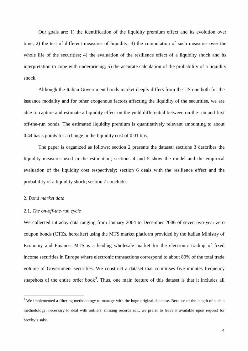
In Table 1, we summarize the seven CTZs used in our study by providing information on
their on- and off-the-run status and on the period during which data are collected. When the first
CTZ is auctioned, it is on-the-run or benchmark until the second CTZ is issued. From that moment
on, the first CTZ becomes first off-the-run. After the third CTZ is issued, it then becomes second
off-the-run, and so on. To simplify the reading we numbered progressively from 1 to 7 our
securities which correspond respectively to the ISIN codes: 347137, 353172, 364676, 369706,
383119, 392699, 405105.
As auctions do not follow a regular schedule, but instead vary between 4 and 8 months, the
period during which a specific note is considered on-the-run or benchmark turns out to be irregular4.
As a result, if we consider the six pairs of on-the-run and off-the-run CTZs available progressively in
the market, the time span of each pair is also irregular and roughly amounts to 3, 4, 8, 6, 7 and 8
months, respectively.
4 Actually CTZs are monthly auctioned but most of these monthly auctions are re-openings of “old” securities.
6
Table 1. On-and off-the run cycle of CTZs
ISIN CODE On/off status From Maturity Data Sample
CTZ 1 347137 1st OFF
2nd
OFF
3rd
OFF
4rd
OFF
10/09/2003
29/03/2004
27/07/2004
24/03/2005
29/04/2005 01/01/2004 – 30/04/2005
CTZ 2 353172 ON
1st OFF
2nd
OFF
3rd
OFF
10/09/2003
29/03/2004
27/07/2004
24/03/2005
31/08/2005 01/01/2004 - 21/08/2005
CTZ 3 364676 ON
1st OFF
2nd
OFF
3rd
OFF
29/03/2004
27/07/2004
24/03/2005
27/09/2005
28/04/2006 24/03/2004 - 28/04/2006
CTZ 4 369706 ON
1st OFF
2nd
OFF
3rd
OFF
27/07/2004
24/03/2005
27/09/2005
24/04/2006
31/07/2006 23/07/2004 - 25/07/2206
CTZ 5 383119 ON
1st OFF
2nd
OFF
24/03/2005
27/09/2005
24/04/2006
30/04/2007 22/03/2005 – 01/12/2006
CTZ 6 392699 ON
1st OFF
2nd
OFF
27/09/2005
24/04/2006
31/12/2006
28/09/2007 23/09/2005 – 29/12/2006
CTZ 7 405105 ON 24/04/2006 30/05/2008 21/04/2006 – 29/12/2006
Total number of quotes in the dataset (in millions) : 2.93;
Total number of contracts: 44387
Now, our first aim is to relate the yield differential of two securities to specific indicators
suitable to measure the different degree of liquidity and so capable to extrapolate from the yield
differential the liquidity premium. Therefore, our next steps are to present the liquidity indicators
adopted and then the evidence of some descriptive statistics of our database on behalf of that we
may asses on the more and less liquid securities and the consequent premium paid for the latter. As
anticipated above, the notes to compare are those contemporaneously exchanged but in a different
condition of liquidity during the on/off cycle. Coherently with the afore mentioned literature and
with the evidence from the descriptive analysis of our database, we choose to compare the security
in the more liquid first off-the-run condition with the less liquid on-the-run one.
2.2 Liquidity indicators
We start our analysis by computing various measures of liquidity of the on-the-run and off-the-run
securities based on both proposals in the order book and transactions. Because the MTS market is a

7
quote-driven electronic order book where quotes are immediately executable, indicators based on
proposals of transactions are particularly relevant to evaluate the liquidity provided by market
makers. Specifically, we use the following proposal-based liquidity measures which have been
found to be significantly relevant in describing market liquidity of Italian Government bonds5:
1. bestspread (bs)= bestaskprice – bestbidprice;
2. weighted spread (ws)= bidweigthbibpriceaskweigthaskprice ** ;
3. slope (steepness to quantity) =
easkbestsizzeaskquotesi
iceworstaskprcebestaskpri
ebidbestsizzebidquotesi
iceworstbidprcebestbidpri 100*100*
2
1
bid or ask quote size = bid or ask quantity ;
4. average quote depth (aqd) =
yaskquantit
askpricemidquote
ybidquantit
midquotebidprice
2
1 , midquote=
2
bidpriceaskprice;
5. market quality index (mqi)= *
*10000
averagequotesize midquote
spread, average quote size (aqs)=
)(2
1ybidquantityaskquantit .
The first two are pure price measures; the third one is considered a price measure as well even if
is in relative terms since it is given by the change in prices upon the change in quantities. The last
two are to be retained as quantity measures because are referred respectively to the depth of the
market from both the supply and demand sides, and to the quality of the market in terms of
averaged quantities and quotes. As usual, the former are positively related with the degree of
liquidity while for the latter the opposite is true. All of them are obtained considering a minute-
snapshot of observations grouped by 5-minutes of trading activity to which best, worst and
averaged (barred) variables refer. This information is then used by averaging through the days of
5 See, in particular, Coluzzi et al. (2008) "Measuring and Analyzing the Liquidity of the Italian Treasury Security
Wholesale Secondary Market", where such measures have been tested highly significant as representative of the
liquidity of the Italian public debt traded in the secondary market.

8
the sample period every five minutes, and through the 5-minutes every day. In the former case we
study what happens in an “average day” in the latter one what happens during the sample period.
It is worth noticing that, as will be argumented later theoretically, we will analyze a liquidity
shock in terms of the associated cost computed in the interest rate. Therefore, we need to build our
indicators (1)-(5) by using the changes at any time both in prices and quantities. Specifically, in
such a way bs and ws will represent respectively the exact and the weighted rate of cost of a
liquidity shock.
As for the measures based on transactions, we analyse the following list of indicators:
6. trading volume (TD)=
100
* icecontractprtradesize
7. trading frequency (TF)= number of contracts
8. net trading count (NTC) = (number of buy contracts – number of sell contracts)
9. net trading quantity (NTQ) = volumesellvolumebuy .
They are respectively volume and frequency measures in levels and differences between supply and
demand sides. These measures are related positively with the degree of liquidity and contribute in
providing evidence on the liquidity path of our securities but will not be used as representative of
the liquidity cost since the conclusion of the contracts, to which they are referred, is subsequent to
the evaluation of the degree of liquidity. Instead, the first five measures rely on the comparison
between the bid and ask sides of the order book, which specifically takes into account this problem.
3. Descriptive Analysis of Liquidity
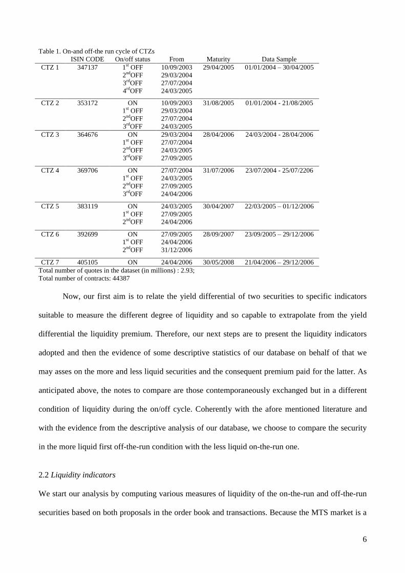
The evolution of liquidity during the whole life of the CTZs is summarized in figures 1 and 2. For
simplicity’s sake, we only focus on one of the securities in our sample, CTZ 3, which we consider
as representative of our database since we have data spanning its entire life. However, similar charts
can be obtained for the other securities.
Looking at the order book measures, we find a sharp difference between the on-the-run and
the off-the-run period. All the order book measures in Figure 1 show that the liquidity of Italian
9
CTZs increases over time. Thus, liquidity in the off-the-run period is higher than in the on-the-run
period. In the case of the two spread measures, our indicators tend to enhance the level of liquidity
in favour of the off-the-run period. However, even the three measures based on depth, average
quote depth, market quality index and slope, show a better performance in the off-the-run period.
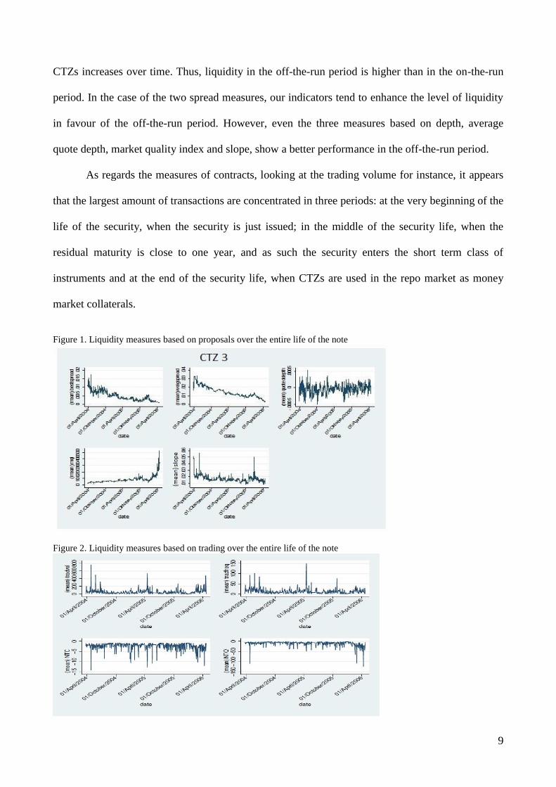
As regards the measures of contracts, looking at the trading volume for instance, it appears
that the largest amount of transactions are concentrated in three periods: at the very beginning of the
life of the security, when the security is just issued; in the middle of the security life, when the
residual maturity is close to one year, and as such the security enters the short term class of
instruments and at the end of the security life, when CTZs are used in the repo market as money
market collaterals.
Figure 1. Liquidity measures based on proposals over the entire life of the note
Figure 2. Liquidity measures based on trading over the entire life of the note
10
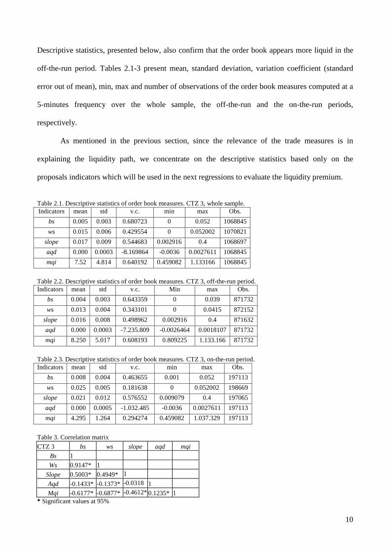
Descriptive statistics, presented below, also confirm that the order book appears more liquid in the
off-the-run period. Tables 2.1-3 present mean, standard deviation, variation coefficient (standard
error out of mean), min, max and number of observations of the order book measures computed at a
5-minutes frequency over the whole sample, the off-the-run and the on-the-run periods,
respectively.
As mentioned in the previous section, since the relevance of the trade measures is in
explaining the liquidity path, we concentrate on the descriptive statistics based only on the
proposals indicators which will be used in the next regressions to evaluate the liquidity premium.
Table 2.1. Descriptive statistics of order book measures. CTZ 3, whole sample.
Indicators mean std v.c. min max Obs.
bs 0.005 0.003 0.680723 0 0.052 1068845
ws 0.015 0.006 0.429554 0 0.052002 1070821
slope 0.017 0.009 0.544683 0.002916 0.4 1068697
aqd 0.000 0.0003 -8.169864 -0.0036 0.0027611 1068845
mqi 7.52 4.814 0.640192 0.459082 1.133166 1068845
Table 2.2. Descriptive statistics of order book measures. CTZ 3, off-the-run period. Indicators mean std v.c. Min max Obs.
bs 0.004 0.003 0.643359 0 0.039 871732
ws 0.013 0.004 0.343101 0 0.0415 872152
slope 0.016 0.008 0.498962 0.002916 0.4 871632
aqd 0.000 0.0003 -7.235.809 -0.0026464 0.0018107 871732
mqi 8.250 5.017 0.608193 0.809225 1.133.166 871732
Table 2.3. Descriptive statistics of order book measures. CTZ 3, on-the-run period. Indicators mean std v.c. min max Obs.
bs 0.008 0.004 0.463655 0.001 0.052 197113
ws 0.025 0.005 0.181638 0 0.052002 198669
slope 0.021 0.012 0.576552 0.009079 0.4 197065
aqd 0.000 0.0005 -1.032.485 -0.0036 0.0027611 197113
mqi 4.295 1.264 0.294274 0.459082 1.037.329 197113
Table 3. Correlation matrix
CTZ 3 bs ws slope aqd mqi
Bs 1
Ws 0.9147* 1
Slope 0.5003* 0.4949* 1
Aqd -0.1433* -0.1373* -0.0318 1
Mqi -0.6177* -0.6877* -0.4612* 0.1235* 1
* Significant values at 95%

11
In the case of the two spread measures, the on-the-run average values are twice the statistics of the
off-the-run period. Also the difference in the mqi is important between the two periods, even though
the volatility of this indicator increases when the security becomes off-the-run.
In Table 3 we calculate the correlation matrix of all the indicators in order to be convinced
of how to interpret our next econometric results. In particular, and as expected, we have the
confirmation that price indicators are –almost all- significantly correlated negatively with the
quantity ones and that, within the two groups of indicators, they are all positively correlated.
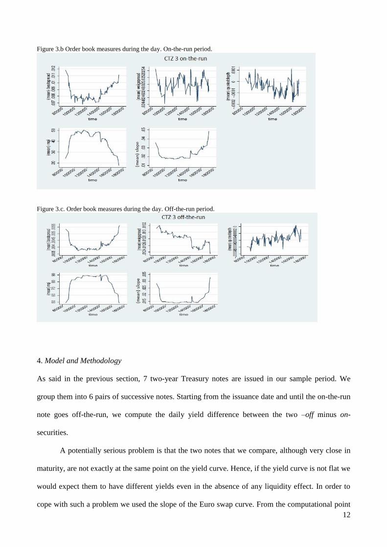
Finally, we analyse the evolution of the order book measures during the trading day. To this
purpose we construct daily average liquidity indicators of every five minutes interval again for the
whole sample (Figure 3.a), the on-the-run and off-the-run periods (Figure 3.b-c). Overall, these
patterns exhibits a U-shaped form especially pronounced for bs and slope while it is inverted, by
index construction, for mqi, where the spread is at the denominator. Thus, as expected, the market is
less liquid at the beginning and at the end of the trading day while it becomes more liquid in the
course of the morning once the opinions of the market makers become more consolidated6.
Also during the day it is discernable a higher liquidity cost to be paid for the on-the-run
security, which confirms the greater liquidity of the Italian public debt in the off-the-run period.
Figure 3.a. Order book measures during the day. Whole sample.
6 In the ws case, liquidity keeps on increasing till the early afternoon, in coincidence with the opening of the US
markets.
12
Figure 3.b Order book measures during the day. On-the-run period.
Figure 3.c. Order book measures during the day. Off-the-run period.
4. Model and Methodology
As said in the previous section, 7 two-year Treasury notes are issued in our sample period. We
group them into 6 pairs of successive notes. Starting from the issuance date and until the on-the-run
note goes off-the-run, we compute the daily yield difference between the two –off minus on-
securities.
A potentially serious problem is that the two notes that we compare, although very close in
maturity, are not exactly at the same point on the yield curve. Hence, if the yield curve is not flat we
would expect them to have different yields even in the absence of any liquidity effect. In order to
cope with such a problem we used the slope of the Euro swap curve. From the computational point
13
of view we subtracted from the yield differential of the two CTZs the difference of their asset swap
spreads7.
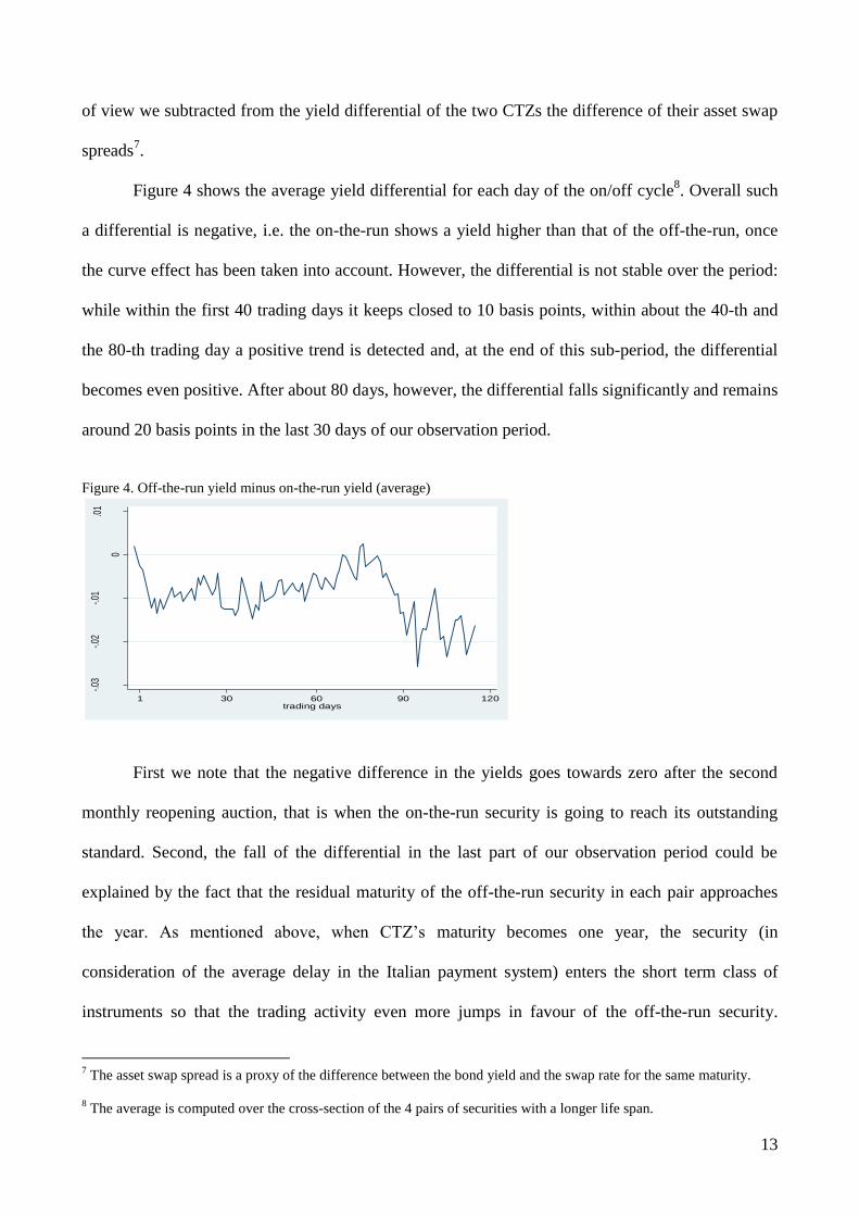
Figure 4 shows the average yield differential for each day of the on/off cycle8. Overall such
a differential is negative, i.e. the on-the-run shows a yield higher than that of the off-the-run, once
the curve effect has been taken into account. However, the differential is not stable over the period:
while within the first 40 trading days it keeps closed to 10 basis points, within about the 40-th and
the 80-th trading day a positive trend is detected and, at the end of this sub-period, the differential
becomes even positive. After about 80 days, however, the differential falls significantly and remains
around 20 basis points in the last 30 days of our observation period.
Figure 4. Off-the-run yield minus on-the-run yield (average)
-.03
-.02
-.01
0
.01
avg
yiel
d di
ffere
nce
1 30 60 90 120trading days
First we note that the negative difference in the yields goes towards zero after the second
monthly reopening auction, that is when the on-the-run security is going to reach its outstanding
standard. Second, the fall of the differential in the last part of our observation period could be
explained by the fact that the residual maturity of the off-the-run security in each pair approaches
the year. As mentioned above, when CTZ’s maturity becomes one year, the security (in
consideration of the average delay in the Italian payment system) enters the short term class of
instruments so that the trading activity even more jumps in favour of the off-the-run security.
7 The asset swap spread is a proxy of the difference between the bond yield and the swap rate for the same maturity.
8 The average is computed over the cross-section of the 4 pairs of securities with a longer life span.

14
Finally, we observe a clear cut downward and upward swing respectively at the very beginning and
end of the yields differential path. This means that immediately after the auction of a new security
its on-the-run return starts increasing while the opposite occurs just before a new on-the-run is
arriving. As found by Lou et al. (2013) for the US liquidity market the explanation resides in the
pressure exerted by the primary dealers when sell analogous securities in the secondary market
before acquiring in Treasury auctions. This fact, together with the imperfect capital mobility due to
the few end-investors and arbitrageurs in the Italian liquidity market, brings to the above stylized
evidence.
However, despite the peculiar behaviour of the yield differential in the Italian Government
bonds market, we are able to detect a liquidity effect on the yield differentials. Now, we briefly
present the theoretical foundation of our econometric analysis.
Theoretical studies show that the yield of a bond is equal to the yield of a perfectly liquid
bond plus a term that captures current and expected future trading costs. Therefore, we estimate an
econometric model where the yield differential of two bonds with different degrees of liquidity
depends just on that:
(1) , ,( )it i off it on it itYD I I
where YDit is the yield spread, ,j itI is the index of liquidity adopted for the security in the j-th (off,
on) state and belonging to the i-th pair at time t, it is the error term.
Provided that the index ,j itI represents “well” the cost of liquidity, equation (1) stems from
the definition of the price of an illiquid bond once the forward rate and the probability that a
liquidity shock hits the bond are taken into account. In fact, if f is the instantaneous forward rate,
PtI the price of an illiquid bond, Pt
L the price for a liquid bond, c the instantaneous cost rate of the
liquidity and the related probability shock, it is true that:
(2)
( )( )
T
t t
f c dc T tI L
t tP e e P
,
T
t
t
C c d , tt
Cc
T t

15
which, in terms of yields is
(3) ( ) ( )( )
I L
t ty T t c y T tI
tP e e
with ( )
T
I
t
t
Y f c d , I
It
t
Yy
T t
, ,
T LLL t
t t
t
YY f d y
T t
where the barred variables, ,L I
tt ty y c , are, for the maturity considered, respectively the average
interest and cost rates associated to the yields of the liquid ( L
tY ) or illiquid ( I
tY ) bond and to the
cost of liquidity shocks (Ct). From (3) it follows that
(4) I L
tt ty c y .
Moreover, if we consider two securities (off and on) with different degrees of liquidity this last
expression becomes
(5) ( )off on off on
t tt ty y c c .
A part for the use of the yields instead of the interest rates, expression (5) is the analogue of the
expression (1).
According to such a scheme we present two estimations.
A first one provides a comparison and is in line with the above cited literature. It defines the
index ,j itI as the time average current and future liquidity measured by the indicators (1)-(5) of the
previous section ( ,j itl ),
(6) , ,
1 T
j it j i
t
l LT t
, , ,
T
j it j i
t
L l
,
Therefore, in this case, accounts also for the time to maturity (T-t), i.e. the estimated coefficient is
referred, with daily data, to a CTZ, of, say, 720 days. As a consequence, once the index ,j itl matches
with the time average cost-rate of liquidity, we need to disentangle the estimation of from the
term of reference in order to assess on the probability of a liquidity shock9.
9 Of course, we may correctly assume the probability as constant notwithstanding T-t diminishes when the time-
average liquidity-indicator approaches to maturity, because also the yield differential, on which the differential of the
mentioned indicator is regressed, varies accordingly.

16
A second estimation will be carried out by considering the summation, Lj,it, of the present
and future liquidity indicators, more coherently with the theoretical background (2)-(5) which
relates such a summation to the yield. In effect, in the literature (see Goldreich et al. , 2005) such an
aspect is not deepened and the concepts of yield and interest rate are interchanged in continuous
time, instead analyzing this point in detail is crucial for the calculation of a reliable probability of
the liquidity shock.
5. Liquidity shocks
5.1 Overall estimates
We estimate equation (1) per each of the five order book measures for the proposals considered in
section 2. As argued above, the smaller are both the spreads and slope, as well as the larger are the
market quality index and the average quoted depth, the more liquid will be the order book. Then, a
fall in the differentials of the spreads or slope indexes and an increase in the differentials of the
quantity indicators are associated with a fall in the yield differential, that means a raise in the
liquidity premium. We therefore expect a positive and negative coefficient for price and quantity
regressors respectively.
We first perform single equation estimations using an econometric model with
autoregressive residuals following Hamilton (1994). Such a methodology, other than to be
consistent to cope with spurious regressions, is specifically suitable with our analysis and in general
with models having independent variables referred to the future because of the autocorrelation
generated in the residuals.
17
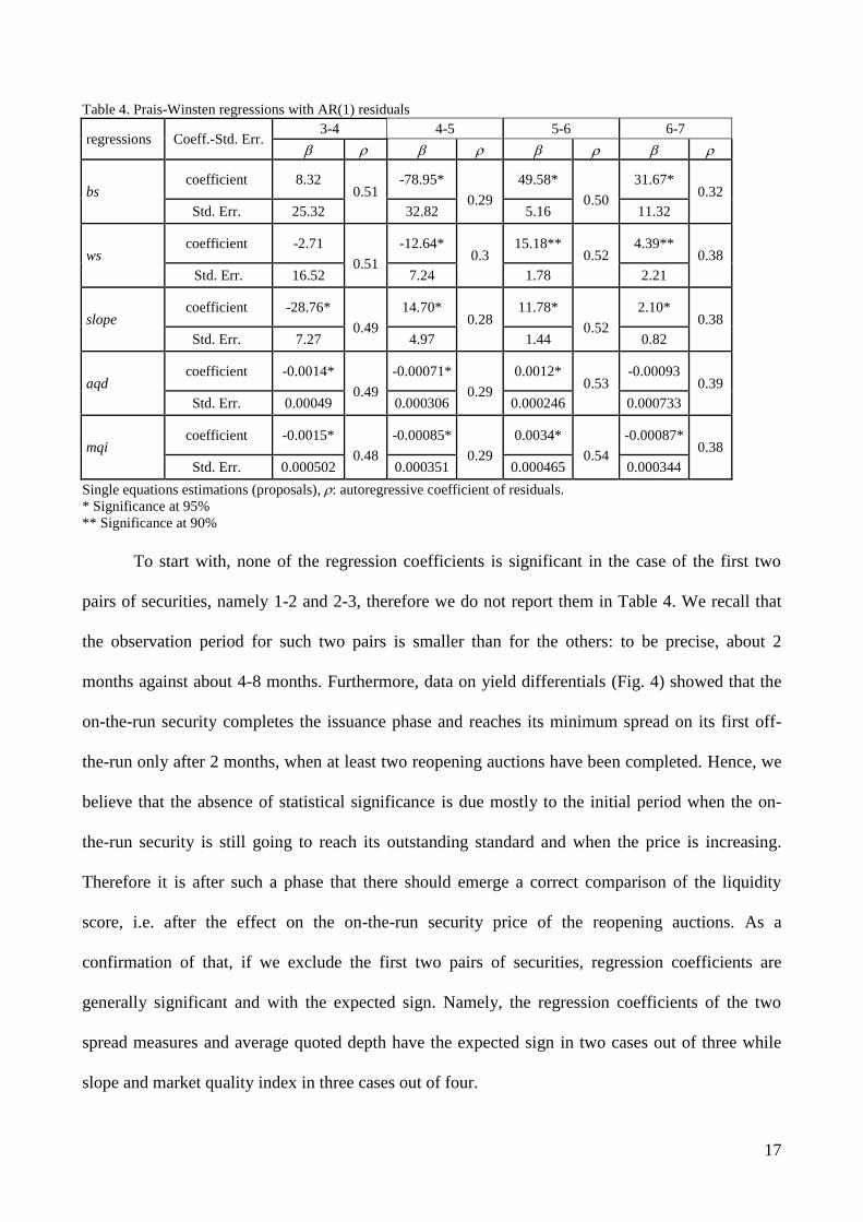
Table 4. Prais-Winsten regressions with AR(1) residuals
regressions Coeff.-Std. Err. 3-4 4-5 5-6 6-7
bs coefficient 8.32
0.51 -78.95*
0.29
49.58*
0.50
31.67* 0.32
Std. Err. 25.32 32.82 5.16 11.32
ws coefficient -2.71
0.51
-12.64* 0.3
15.18** 0.52
4.39** 0.38
Std. Err. 16.52 7.24 1.78 2.21
slope coefficient -28.76*
0.49
14.70* 0.28
11.78*
0.52
2.10* 0.38
Std. Err. 7.27 4.97 1.44 0.82
aqd coefficient -0.0014*
0.49
-0.00071*
0.29
0.0012* 0.53
-0.00093 0.39
Std. Err. 0.00049 0.000306 0.000246 0.000733
mqi coefficient -0.0015*
0.48
-0.00085*
0.29
0.0034*
0.54
-0.00087* 0.38
Std. Err. 0.000502 0.000351 0.000465 0.000344
Single equations estimations (proposals), : autoregressive coefficient of residuals.
* Significance at 95%
** Significance at 90%
To start with, none of the regression coefficients is significant in the case of the first two
pairs of securities, namely 1-2 and 2-3, therefore we do not report them in Table 4. We recall that
the observation period for such two pairs is smaller than for the others: to be precise, about 2
months against about 4-8 months. Furthermore, data on yield differentials (Fig. 4) showed that the
on-the-run security completes the issuance phase and reaches its minimum spread on its first off-
the-run only after 2 months, when at least two reopening auctions have been completed. Hence, we
believe that the absence of statistical significance is due mostly to the initial period when the on-
the-run security is still going to reach its outstanding standard and when the price is increasing.
Therefore it is after such a phase that there should emerge a correct comparison of the liquidity
score, i.e. after the effect on the on-the-run security price of the reopening auctions. As a
confirmation of that, if we exclude the first two pairs of securities, regression coefficients are
generally significant and with the expected sign. Namely, the regression coefficients of the two
spread measures and average quoted depth have the expected sign in two cases out of three while
slope and market quality index in three cases out of four.

18
We also underline that the constant terms, not reported here for brevity, are all very close to
0 in accordance with the theory of the previous section which, in case of two identical notes but
liquidity, attributes the difference in the yield only to the cost-rate of a liquidity shock, thus
excluding fixed effects.
The yield premium amounts to about a quite consistent 0.31-0.49 basis points for one
percentage basis point rise of the spread if we consider the best spread as a cost indicator10
.
Note that in such estimations the autocorrelation coefficients of residuals are almost identical for the
same pair through the several liquidity indicators and different across pairs. Such an evidence
confirms from one side that actually the indicators presented have the same explicative meaning in
terms of liquidity11
, even if built on different bases (prices and quantities), and from the other side
reveals that the errors structure characterizes the differences between pairs, which is important in
order to go further with the empirical research of the panel coefficients across securities. Panel
analysis is especially needed as regards price indicators, and in particular the best spread, in order to
check if a unique and reliable coefficient of the cost-rate of liquidity is retrievable.
5.2 Liquidity cost
Now, in order to identify the liquidity cost effect for a representative pair of securities, we present,
in the following Table 5, the panel regressions on prices indicators12
. For what explained above we
10
Such an impact falls to the interval 0.04-0.15 basis points if we refer to the weighted spread. However, this one is a
less precise measure of the cost of liquidity since accounts for other elements, a part from prices, in its calculation.
11 With the same methodology we carried out also rolling regressions obtaining similar paths for the coefficients of the
several liquidity indicators, that is coherent again, notwithstanding the intrinsic differences, with the common meaning
of liquidity they have.
12 However, for completeness, we made also a panel regression for the quantities indicators but, in such a case, a
stronger variability across securities has been found and a specific security effect on the coefficients for each measure
has been revealed necessary to obtain good results, which deprives of utility the panel estimation.
19
consider autoregressive errors and adopt the FGLS regression method to allow for an error-
covariance matrix across pairs of general form.
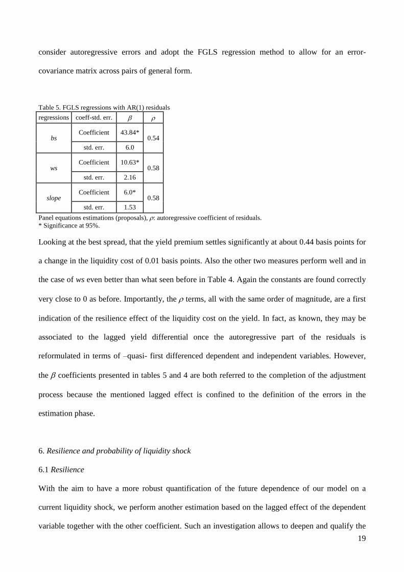
Table 5. FGLS regressions with AR(1) residuals
regressions coeff-std. err.
bs Coefficient 43.84*
0.54
std. err. 6.0
ws Coefficient 10.63*
0.58
std. err. 2.16
slope Coefficient 6.0*
0.58
std. err. 1.53
Panel equations estimations (proposals), : autoregressive coefficient of residuals.
* Significance at 95%.
Looking at the best spread, that the yield premium settles significantly at about 0.44 basis points for
a change in the liquidity cost of 0.01 basis points. Also the other two measures perform well and in
the case of ws even better than what seen before in Table 4. Again the constants are found correctly
very close to 0 as before. Importantly, the terms, all with the same order of magnitude, are a first
indication of the resilience effect of the liquidity cost on the yield. In fact, as known, they may be
associated to the lagged yield differential once the autoregressive part of the residuals is
reformulated in terms of –quasi- first differenced dependent and independent variables. However,
the coefficients presented in tables 5 and 4 are both referred to the completion of the adjustment
process because the mentioned lagged effect is confined to the definition of the errors in the
estimation phase.
6. Resilience and probability of liquidity shock
6.1 Resilience
With the aim to have a more robust quantification of the future dependence of our model on a
current liquidity shock, we perform another estimation based on the lagged effect of the dependent
variable together with the other coefficient. Such an investigation allows to deepen and qualify the
20
crucial aspect of the resilience whose importance in the present context is in the possibility of
forecasting the effect of a liquidity shock on the quoted yield. Since we are at the presence of high
time frequency data and a small number of units (securities) the straightforward method is that of
the GMM Arellano-Bond dynamic estimator13
,
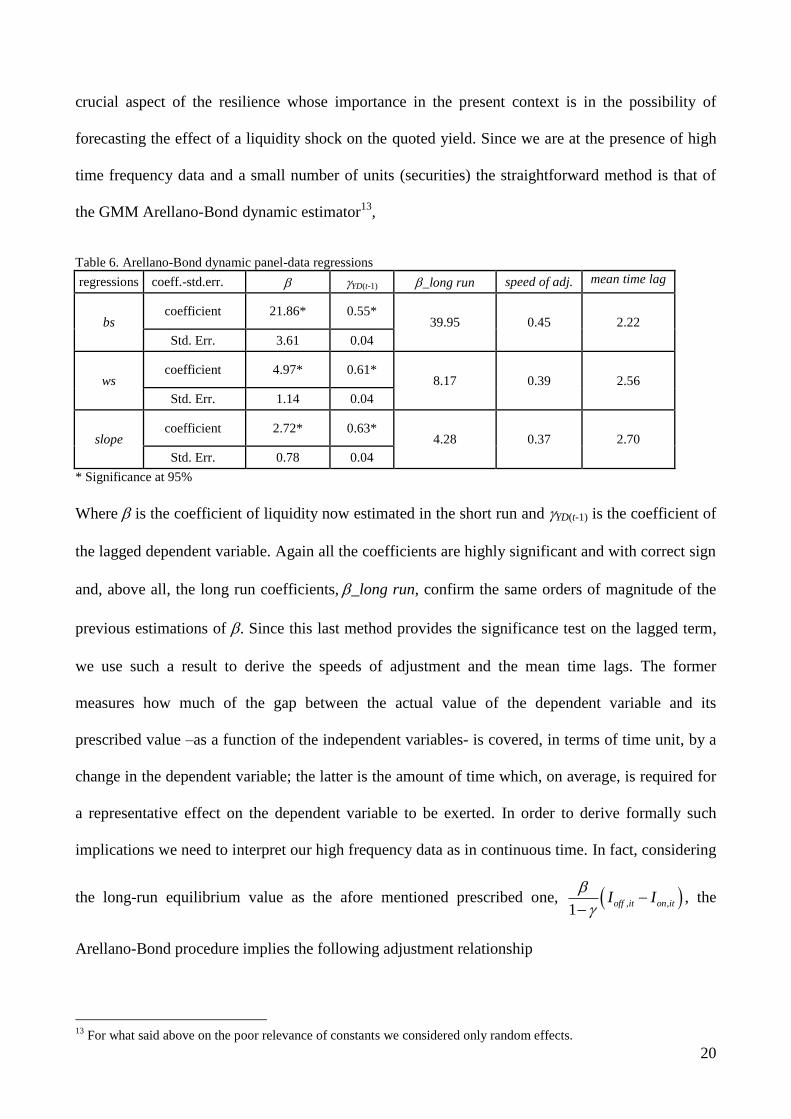
Table 6. Arellano-Bond dynamic panel-data regressions
regressions coeff.-std.err. YD(t-1) _long run speed of adj. mean time lag
bs coefficient 21.86* 0.55*
39.95 0.45 2.22
Std. Err. 3.61 0.04
ws coefficient 4.97* 0.61*
8.17 0.39 2.56
Std. Err. 1.14 0.04
slope coefficient 2.72* 0.63*
4.28 0.37 2.70
Std. Err. 0.78 0.04
* Significance at 95%
Where is the coefficient of liquidity now estimated in the short run and YD(t-1) is the coefficient of
the lagged dependent variable. Again all the coefficients are highly significant and with correct sign
and, above all, the long run coefficients,_long run, confirm the same orders of magnitude of the
previous estimations of . Since this last method provides the significance test on the lagged term,
we use such a result to derive the speeds of adjustment and the mean time lags. The former
measures how much of the gap between the actual value of the dependent variable and its
prescribed value –as a function of the independent variables- is covered, in terms of time unit, by a
change in the dependent variable; the latter is the amount of time which, on average, is required for
a representative effect on the dependent variable to be exerted. In order to derive formally such
implications we need to interpret our high frequency data as in continuous time. In fact, considering
the long-run equilibrium value as the afore mentioned prescribed one, , ,1
off it on itI I
, the
Arellano-Bond procedure implies the following adjustment relationship
13
For what said above on the poor relevance of constants we considered only random effects.
21
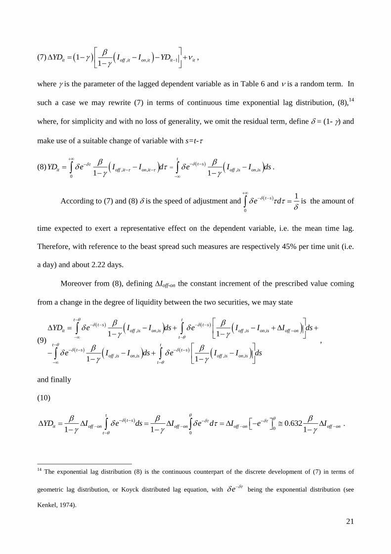
(7) , , 111
it off it on it it itYD I I YD
,
where is the parameter of the lagged dependent variable as in Table 6 and is a random term. In
such a case we may rewrite (7) in terms of continuous time exponential lag distribution, (8),14
where, for simplicity and with no loss of generality, we omit the residual term, define = (1- ) and
make use of a suitable change of variable with s=t-
(8) , ,
01
it off it on itYD e I I d
=
, ,1
tt s
off is on ise I I ds
.
According to (7) and (8) is the speed of adjustment and
0
1t se d
is the amount of
time expected to exert a representative effect on the dependent variable, i.e. the mean time lag.
Therefore, with reference to the beast spread such measures are respectively 45% per time unit (i.e.
a day) and about 2.22 days.
Moreover from (8), defining Ioff-on the constant increment of the prescribed value coming
from a change in the degree of liquidity between the two securities, we may state
(9)
, , , ,
, , , ,
1 1
1 1
t tt s t s
it off is on is off is on is off on
t
t tt s t s
off is on is off is on is
t
YD e I I ds e I I I ds
e I I ds e I I ds
,
and finally
(10)
00
0.6321 1 1
tt s
it off on off on off on off on
t
YD I e ds I e d I e I
.
14
The exponential lag distribution (8) is the continuous counterpart of the discrete development of (7) in terms of
geometric lag distribution, or Koyck distributed lag equation, with e being the exponential distribution (see
Kenkel, 1974).

22
In (10) we move back to the original variable and, in order to discern how quantitatively
“relevant” is the effect of an impulse from a change in the prescribed value within the mean time
lag, impose .We may conclude that the mean time lag represents the time required to close
around the 63% of the gap between the actual and the prescribed value. The mean time lag applied
to our estimation15
therefore represents a clear indication of the resilience due to the cost of the
liquidity. According to this finding, we now know that, such a cost is incorporated in great deal in
the yield within the first 2-3 days and that the increase, which we may forecast per each following
day, is the 45% of the remaining gap.
Such a result has important implications also to cope with problems of Treasury-auctions
efficiency-designs related to underpicing. Lou et. al (2013), claim the necessity of understanding
how much of the initial upward swing in the price, due to the liquidity shock caused by auction,
might be exploited by the Treasury or, in the other way round, how much of the cost, due to a
feasible lower yield, might be saved. We may state that the 63% of the liquidity shock, induced by
the primary dealers in the secondary market before (selling) and after (buying) the auction, is
absorbed on average by the price of the new on-the-run security in a span of 1
2.2 time units.
Therefore, according to the amount of issuance, appropriate auctions should be scheduled taking
into account such a frequency.
In Table 7 below we report the observed actual lag, the issuance amount and, as a
consequence, the possible costs savings. The above mentioned lag is evaluated as numbed of the
days necessary for the realization of the largest reduction in the yield since the new security
issuance date.
15
See Gandolfo (1981) for an extended exposition of these problems in a more general context where the aim is to find
the correspondence between stochastic difference and differential equations.
23
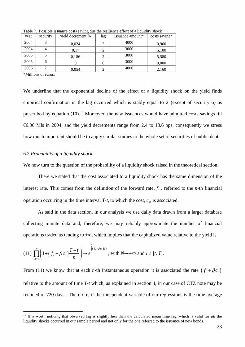
Table 7. Possible issuance costs saving due the resilience effect of a liquidity shock
year security yield decrement % lag issuance amount* costs saving*
2004 3 0,024 2 4000 0,960
2004 4 0,17 2 3000 5,100
2005 5 0,186 2 3000 5,580
2005 6 0 0 3000 0,000
2006 7 0,054 2 4000 2,160
*Millions of euros.
We underline that the exponential decline of the effect of a liquidity shock on the yield finds
empirical confirmation in the lag occurred which is stably equal to 2 (except of security 6) as
prescribed by equation (10).16
Moreover, the new issuances would have admitted costs savings till
€6.06 Mls in 2004, and the yield decrements range from 2.4 to 18.6 bps, consequently we stress
how much important should be to apply similar studies to the whole set of securities of public debt.
6.2 Probability of a liquidity shock
We now turn to the question of the probability of a liquidity shock raised in the theoretical section.
There we stated that the cost associated to a liquidity shock has the same dimension of the
interest rate. This comes from the definition of the forward rate, f , referred to the n-th financial
operation occurring in the time interval T-t, to which the cost, c, is associated.
As said in the data section, in our analysis we use daily data drawn from a larger database
collecting minute data and, therefore, we may reliably approximate the number of financial
operations traded as tending to +∞, which implies that the capitalized value relative to the yield is
(11)
1
1
T
t
f c dN
n
T tf c e
n
, with N→+∞ and τ [t, T].
From (11) we know that at each n-th instantaneous operation it is associated the rate f c
relative to the amount of time T-t which, as explained in section 4, in our case of CTZ note may be
retained of 720 days . Therefore, if the independent variable of our regressions is the time average
16
It is worth noticing that observed lag is slightly less than the calculated mean time lag, which is valid for all the
liquidity shocks occurred in our sample period and not only for the one referred to the issuance of new bonds.

24
rate-of-cost of liquidity, the resulting estimate of is the total probability that in the period T-t
occurs only one liquidity shock, evaluated on average as ,j itl and conditional to time t. Considering
the best spread and dividing by the above mentioned term of reference we obtain
,
T
j it
t t
P l
T t
=
6.09%, which is a measure of the daily probability of a liquidity shock in such a case.
Differently, more closely to the expressions of the yield (3) and (11), we may regress the
yield differential on the differential of the summation of the current and future liquidity indicators.
In such a case is to be interpreted as the joint probability of all daily liquidity shocks occurrences
spanned through maturity.
The results, reported in Table 8, are relative to all the indicators and securities and confirm
the underlying theory. In fact, the pair 6-7 provides good results for prices measures when the
regressions are based on the average liquidity indicators (Table 4) but not in this case where there
appear wrong signs except for slope. Actually, such a pair has the longest on/off cycle but the
shortest observation period which does not cover the term of the two securities. Therefore, in this
case, the calculation of the joint probability is not satisfactory because the indicators used are not
representative of the cumulative sum of the liquidity shocks to maturity, instead the total probability
coefficient is significantly related to the average cost, which revealed representative of the daily
shock of liquidity.
Table 8. Prais-Winsten regressions with AR(1) residuals
regressions coeff.-std. err. 3-4 4-5 5-6 6-7
bs coefficient 0.000305*
0.48 0.00013*
0.30 0.00237*
0.54 -0.0000531*
0.38
Std. Err. 0.000103 5.31E-05 0.000282 0.0001617
ws coefficient 0.000128*
0.48 0.000067*
0.30 0.000951*
0.54 -5.20E-06*
0.38
Std. Err. 4.26E-05 2.71E-05 0.000111 0.0000366
slope coefficient 0.000129*
0.48 9.11E-05*
0.30 -0.00018*
0.55 0.0014547*
0.30
Std. Err. 4.08E-05 3.93E-05 2.43E-05 0.000303

25
aqd coefficient -8.68E-09*
0.48 -9.64E-09*
0.30 -1.56E-08*
0.55 -5.68E-10*
0.38
Std. Err. 2.82E-09 4.32E-09 1.96E-09 2.31E-09
mqi coefficient -8.99E-09*
0.48 -5.67E-09*
0.30 -2.36E-08*
0.54 -1.75E-09*
0.38
Std. Err. 2.90E-09 2.43E-09 2.95E-09 2.14E-09
Single equations estimations (proposals), : autoregressive coefficient of residuals.
* Significance at 95%
It is worth noticing that, apart for slope in the pair 5-6 and the two spreads in the pair 6-7 for the
afore mentioned reasons, all the other indicators, included the quantity ones, are significant and
with correct sign, which is certainly better than what obtained in Table 4 and provides the empirical
validation of the theory developed in section 4. From Table 8 the liquidity-shocks composed-
probability associated to the cost of the best spread goes from 0.013% to 0.24% according to the
security considered. However, to be more precise, we perform also in this case a panel regression
using the same procedure of section 5.2 and obtain again significant results at 95% level for the best
and weighted spread while for slope the sign of the coefficient is not correct but very close to 0 and
less significant17
.
Table 9. FGLS regressions with AR(1) residuals
regressions coeff-std. err.
bs Coefficient 0.00030*
0.57
std. err. 0.000081
ws Coefficient 0.00014*
0.55
std. err. 0.000031
slope Coefficient -0.000050**
0.65
std. err. 0.000020
Panel equations estimations (proposals), : autoregressive coefficient of residuals.
* Significance at 95%, ** Significance at 90%.
17
The result of a coefficient approaching 0 for slope in this panel estimation is rather expected because it is a more
unstable measure (given by the ratio between small values). This is also confirmed by the highest autoregressive
coefficient for residuals. Differently, in the panel regression of Table 5 the averaged over time measure used for slope is
more stable and allows to identify a correct result across the pairs of securities.

26
According to such an estimation, the joint probability conditional to time t and associated with the
cost of the best spread amounts to ,
T
j it
t
P l
= 0.03%. As expected, given the meaning of joint
probability, such a value is definitely smaller the one of the daily total probability.
To conclude, even if the Italian Government bonds market is characterized by its own
peculiarities, such as specific issuance modalities or taxation, a liquidity shock effect has been
found on all the five order book measures we considered. Given that the estimated liquidity
premium is quantitatively relevant, further research would be needed in order to evaluate: 1) the
change in the liquidity shock probability over time, 2) an appropriate scheduling system of the new
issuances to save the costs due to the liquidity shock resilience, 3) if the liquidity premium is
present on other securities not considered in our analysis.
7. Conclusions
This research focuses on the premium of liquidity for the Italian Government bonds. To this aim we
used indexes of liquidity belonging to both the categories of price and quantity. We then examine
such indicators for the entire life of the securities considered both for descriptive purposes and for
estimation. On this last point we regress the yield differential, between a pair of securities off- and
on-the-run, on the several indicators under exam. In doing so we refer to the present and future
liquidity and, for this reason, to the expectation on the mentioned indexes. We concentrate our
attention on the two-years-CTZ-notes in order to avoid coherence problems due to differences in
coupons when comparing different securities. We perform both single and panel regressions per
each indicator and emphasize the necessity of a specific analysis to better interpret the
characteristics of the Italian market. We find an important liquidity premium associated to the
corresponding probability and a significant resilience effect which allows to characterize better the
underpricing phenomenon. Finally, we underline the necessity to the extend the analysis here
developed also to the other securities of the public debt.
27
Acknowledgments
We are grateful to the Italian Public Debt Department at the Ministry for Economy and Finance for
the support given and for extremely helpful suggestions and comments. We thank Chiara Coluzzi,
Tiziana Capponi, Davide Iacovoni, Paola Fabbri, Paola De Rita, Sergio Ginebri, Manuel Turco and
Stefano Fachin. Finally, we thank Christine Parlour and Antonio Scalia for their contribution at the
presentation of a preliminary version of this paper at the Ministry of Economy and Finance. We
also thank the University of Rome “La Sapienza” and MIUR for having provided research funds on
this topic. The usual disclaimer always applies.
References
Alonso F., Blanco R., del Rio A. Sanchis A. (2000), Estimating Liquidity Premia in the Spanish
Government Securities Market, Banco de Espana, Servicio de Estudios, Documento de Trabajo n°
0017.
Amihud Y. and Mendelson H (1991), Liquidity, Maturity and the Yield on the US Treasury
Securities, Journal of Finance, 46, 1411-1425.
Amihud Y.(2001), Illiquidity and Stock Returns: Cross-section and Time-series Effects, Journal of
Financial Markets 5, 31-56
Balduzzi P., Elton J. and Green T. C. (2001), Economic News and Bond Prices: Evidence from the
US Treasury Market, Journal of Financial and Quantitative Analysis, 36, 523-543.
28
Coluzzi, C., Delle Chiaie, S., Ginebri, S., Maggi, B., Turco M., (2008) Measuring and Analyzing
the Liquidity of the Italian Treasury Security Wholesale Secondary Market, Ministry of Economy
and Finance Report, Italy (2008).
Elton E. J., Green T. (1998), Tax and Liquidity Effects in Pricing Government Bonds, Journal of
Finance, 53, 1533-1562.
Favero, C., Pagano M., von Thadden E. L. (2005), Valuation, Liquidity and Risk in Government
Bond markets, unpublished paper.
Fleming M. J. and Remolona E. M. (1999), Price Formation and Liquidity in the US Treasury
Market: The Response to Public Information, Journal of Finance, 54, 1901-1916
Fleming M. J. (2003), Measuring Treasury Market Liquidity, Federal Reserve Bank of New York
Economic Economic Policy Review (September), 83-108
Gandolfo, G. (1981), “Qualitative Analysis and Econometric Estimation of Continuous Time
Dynamic Models”, North Holland.
Garbade K. D. (1996), Fixed Income Analysis, MIT Press, Cambridge, Mass.
Goldreich, D., Hanke B., Nath P. (2005), The Price of Future Liquidity: Time-Varying
Liquidity in the U.S. Treasury Market, Review of Finance 9(1), 1-32.
Hamilton, J. (1994), Time Series Analysis, Princeton University Press.

29
Kamara A. (1994), Liquidity of the Government of Canada Securities Market: Stylised Facts and
some Market Microstructure Comparisons to the United States Treasury Market, Bank of Canada,
Working Paper 99-11.
Kenkel, J. L., (1974), Dynamic Linear Economic Models, Gordon and Breach, New York.
Lou D, Yan H., Zang J. (2013), Anticipated and Repeated Shocks in Liquid Markets, The Review of
Financial Studies, n° 26 (8), pp. 1891-1912.
Maggi, B, Infortuna F. (2008), Assessing Italian Government Bonds Term Structure with CIR model
in the aftermath of EMU, Applied Financial Economic Letters, Volume 4, Issue 3, pp. 163 – 170.
Nelson C. R. and Siegel A. F. (1987), Parsimonious Modelling of Yield Curves for US Treasury
Bills, Journal of Business, 60, 473-489.
Pasquariello P., Vega C. (2009), The on-the-run liquidity phenomenon, Journal of Financial
Economics, 92, 1-24.
Recommended


![[Journal] the Effect of Debt, Firm Size and Liquidity on Investment](https://img.pdfslide.us/doc/110x75/577cc4d01a28aba7119a8653/journal-the-effect-of-debt-firm-size-and-liquidity-on-investment.jpg)