Is There a Self-fulfilling Prophecy in Credit Rating
Announcements?*
Paulo Viegas Carvalho
Department of Finance, ISCTE-IUL Business School, Lisboa
email: [email protected]
Paul Anthony Laux
Department of Finance, University of Delaware, Newark, Delaware
email: [email protected]
João Pedro Pereira
Department of Finance, ISCTE-IUL Business School, Lisboa
email: [email protected]
This version: January, 2014
Abstract
Although credit ratings are meant to foretell a firm’s risk of default, anecdotal evidence suggests that they
actually influence the firm’s probability of default. This paper provides systematic evidence on this unintended
effect of rating downgrades on future credit defaults. Based on complementary causality methodologies and
using an exhaustive database of long-term corporate obligation ratings issued by Moody’s, S&P and Fitch, from
1990 to 2011, the paper shows that downgrades crossing the threshold between investment grade and speculative
grade cause an increase of at least 3% in the 1-year probability of default. Naturally, the increase in the
probability of default is stronger for deeper rating downgrades. The effect is also stronger for firms that already
have a low initial rating.
JEL classification: C31; C53; D83; G24; G32
Keywords: Treatment effect models; Forecasting; Information; Credit rating agencies; Corporate default
* Financial support by FCT’s research grant PTDC/EGE-GES/119274/2010 is gratefully acknowledged.

2
1. Introduction
The concept of self-fulfilling prophecy is described by Merton (1968, p. 367) as a situation
whereby an incorrect belief or expectation brings forth a new behavior that eventually causes
the original false conception to come true. For example, he uses a parable of a bank with a
stable financial structure that suddenly faces unfounded rumours of insolvency. As the
rumours spread, depositors become increasingly anxious, ultimately leading the bank into
bankruptcy.
The relation between credit ratings and credit default is a similar example. Credit ratings
are meant to foretell the future payment behaviour of the rated firm and to lessen information
asymmetry between that firm and investors. However, rating announcements may as well
generate non-negligible effects on the firm concerned, such as its cost of debt, among other
impacts.1 When these announcements are negative and convey substantial bad news about the
rated firm, they may generate not just temporarily debt cost effects. Instead, longer lasting
consequences that restrain the firm’s financial management and stability may emerge. Such
announcements are likely to undermine investors’ confidence in the firm and strongly
stimulate the proportion of investors anticipating a firm’s default, so withdrawing credit. The
resulting credit restrictions potentially spark liquidity crises that can jeopardize the firm’s
ability to honor its future financial commitments and push it towards credit default; just like
in Merton’s parable. Given the widespread use of credit ratings, it is fundamental to
investigate this potential effect of ratings on credit default.
The purpose of this paper is to study the hypothesis that rating downgrades increase the
probability of default. The obvious difficulty is to disentangle the cause from the effect.
Indeed, as some firms might be so financially fragile that they would have defaulted
regardless of having been downgraded or not, it is not trivial to separate the potential causal
effects we are investigating from ratings’ prediction accuracy. Ex post, we realize what
happened to firms with negative ratings announcements; however, we do not know what
would have happened ceteris paribus to the same firms in the absence of such
announcements. In other words, we observe the factual outcome but not the counterfactual,
which generates a missing data problem as defined by Holland (1986).
It is not strange therefore that related literature does not test the possibility of credit rating
announcements turning into self-fulfilling prophecies of default. For example, Bannier and
1 For example, Ederington and Goh (1998) find that equity analysts are likely to adjust earnings forecasts
“sharply downward” after a downgrade.

3
Tyrell (2006) admit that a wide early withdrawal of credit access pushes the firm into default.
As a result, Kuhner (2001) postulate that some negative credit rating announcements may turn
into self-fulfilling prophecies. This hypothesis is even admitted by Moody’s (Fons, 2002),
which acknowledges “that its ratings can potentially become self-fulfilling forecasts” in the
case of negative announcements, where higher capital costs are expected and restrictions to
the issuer’s access to funding may arise; possibly, these circumstances might even lead to
default. We extend this line of research by testing the conjectures raised in these papers.
This paper uses a threefold econometric approach. Based on Shumway (2001), the first
approach consists in a credit default prediction model which includes rating covariates,
controlling for several default-related variables. We acknowledge that this is a naïve approach
to causality; as ratings also track the probability of default, endogeneity is not precluded here.
However, this analysis helps us clarify our research hypotheses. In addition, it complements
the results obtained using two methods of causality analysis, our second and third approaches.
The second approach lies in the propensity score matching technique proposed by Rosenbaum
and Rubin (1983). The utilization of this method to answer causality problems similar to ours
proliferates in distinct fields of scientific research, such as biology, medicine, economics and
sociology. The third approach, the Heckman treatment effects approach, or Heckit model
(Heckman, 1978, 1979; Maddala, 1983, p. 120), controls for the plausible endogeneity of the
rating announcement; it represents therefore a valuable alternative to the credit default
prediction model. Interestingly, although the three previous approaches imply distinct
methodologies, their results are quite consensual.
Relying on an extensive database of ratings issued by Fitch, Moody’s and Standard &
Poor’s, between 1990 and 2011, the paper confirms that some rating downgrades aggravate
the risk of default. Such is the case of ratings moving from investment grade to speculative
grade, which causes an increase over 3% in the 1-year probability of default when it occurs.
The effect is even larger when we observe downgrades from a level that is already speculative
to another one at best equal to a highly speculative grade; the causality effect in the 1-year
probability of default strengthens in this case to, at least, 12.13%. In addition, the magnitude
of the rating change is found to cause significant effects too. One interpretation for these
significant effects of rating downgrades, in line for example with Gonzalez et al. (2004) and
Jorion et al. (2005), is that ratings convey significant information to the markets. In view of
the results in the current paper, were seemingly abnormal reactions in the rate of default
emerge when rating news are negative, another probable explanation is that such news could
also add noise that affects the firm’s financial performance.

4
The reputation of rating agencies depends on their ability to anticipate future situations of
credit default by assigning them worse rating levels. For example, as stated by Güttler and
Wahrenburg (2007), the higher the ability of a rating agency to anticipate upcoming defaults,
the higher will be its reputation. For not being able to timely anticipate some of the largest
credit failures, especially after the financial markets volatility since the end of the 1990’s, the
three major rating agencies have been the target of some bitter criticism. The most cited
examples are the failures of Enron in 2001, Worldcom and Adelphia Communications
Corporation in 2002, Parmalat in 2003, Lehman Brothers in 2008, as well as the failures of
sovereign issuers (Asian countries in 1997, Russia Federation in 1998, and Argentina in
2001), and of some mortgage-related securities during the subprime crisis of 2007-2008.
Indeed, when assessing credit risk, it is rather important to evaluate to what extent the
underlying assessment tool is able to anticipate default events. Put in another way, the hit rate
or true positives for that tool should remain high and the false negatives or type II error (i.e.
defaults predicted as non-defaults) should be kept low.
An implication from our findings is that it is equally important to evaluate if overly
pessimistic ratings do not unduly penalize borrowers. This means that the misclassification
rate due to false positives or type I error (i.e. non-defaults predicted as defaults) must also be
minimal. Otherwise, with a downward bias in credit decisions, creditors themselves will lose
profitable business opportunities. In addition, regardless of the reasoning behind the detected
effects, a natural consequence from the evidence in this paper appears to be that rating
information, if added to the covariates of statistically-based credit default prediction models,
improves the accuracy of these models.
It is relevant to underline a potential limitation to our conclusions. The study analyses only
public information, but there is also a non-negligible amount of private information that rating
agencies may incorporate in their ratings. It may be that, based alone on public information,
the firm denotes a low risk of default, but the correspondent rating could already reflect
private information that imply an almost unavoidable event of default. Similar limitations are
present in other causality problems, given their underlying missing data problems. By using a
threefold econometric approach, we hope to mitigate this limitation to some extent.
The rest of the paper is organized as follows. Section 2 provides an overview of the main
determinants behind the different rating levels, and highlights the already identified financial
effects and information content of credit ratings. This section contains as well the results of
our credit default prediction model, paving the way to research hypotheses. Section 3
describes the data used for analysis, and reports selected descriptive statistics. Section 4
5
contains an overview of the causality methodologies employed to investigate the hypotheses;
the results obtained are also detailed and discussed here. Section 5 concludes.
2. The relation between ratings and default
This section is divided into three subsections. The first describes some of ratings’ main
features and draws from previous literature to summarize credit ratings’ financial and non-
financial determinants; financial effects of rating announcements are also outlined here. The
second subsection explores a preliminary analysis on the question raised in this paper. This
analysis allows us to postulate research hypotheses in the third subsection.
2.1. Literature review
2.1.1. Credit ratings and their determinants
A credit rating is an independent opinion, whether solicited or unsolicited, on the relative
ability and willingness of a party with debt obligations to meet its financial commitments
(OECD, 2010). Based on public and, in some cases, private information, ratings are assigned
by credit analysts as an ordinal and qualitative measure of risk that in most cases reflects the
long-term credit strength of the rated party. Rating agencies assign corporate credit ratings
either to debt issuers or to particular debt obligations undertaken by those issuers.2
In addition to the publicly available information that unsolicited credit ratings reflect,
solicited ratings also incorporate private information that otherwise exposed would jeopardize
the strategy of the rated company. The research in this paper focuses on the second type of
ratings, based on information about the three main agencies, Standard & Poor’s Credit Market
Services (S&P), Moody’s Investor Services (Moody’s) and Fitch, Inc. (Fitch).3 Dealing with
both public and private information, Standard & Poor’s (2011) groups in two categories the
factors weighed to determine credit ratings: the business risk and the financial risk. Examples
2 Generally, a credit rating reflects the creditworthiness of the issuer, rather than the credit quality of its debt
obligations. An issuer or an obligation may be rated by more than one agency, a circumstance more likely for
large and experienced issuers, as referred by Cantor and Packer (1997). 3 Together, the three agencies dominate the worldwide market: S&P and Moody’s hold approximately 80% of
the market, while Fitch owns 14% (Langohr and Langohr, 2008, p. 386). Such level of concentration confirms
the oligopolistic structure of this market (OECD, 2010), primarily nourished by large barriers to entry. For
instance, Bolton et al. (2012) call an “artificial barrier” the creation of the Nationally Recognized Statistical
Rating Organizations, the designation adopted by the Securities and Exchange Commission for the agencies
whose ratings are valuable for investments decisions.

6
of such factors are the country risk, industry characteristics, company position, risk tolerance,
profitability, governance, capital structure and financial policy.
Though private information limits the investigation of a few of these factors, namely those
obtained by the agencies via private meetings with management, some papers explore the
main observable variables that influence credit ratings. This is the case in Cantor and Packer
(1997), Blume et al. (1998), Amato and Furfine (2004), Kisgen (2006), Güttler and
Wahrenburg (2007), and Jorion et al. (2009). Given that, ultimately, each rating level denotes a
rank relative to other rating levels, such papers generally use ordered multinomial probit or
logit estimations, from where they identify the main variables or factors determining credit
ratings, as presented in Table 1. Due to the unobservable variables inherent to the rating
process, Kamstra et al. (2001) confirm that these estimation methods tend to correctly
forecast, at best, only circa 78% of the observed ratings.
Table 1 shows a digest of explanatory variables reported in previous literature on credit
ratings. The table reveals that different references select four accounting ratios, commonly
computed as:
- Interest coverage: Sum of Operating Income After Depreciation and Interest Expense
divided by Interest Expense;
- Operating margin: Operating Income Before Depreciation divided by Net Sales;
- Long term debt leverage: Total Long Term Debt divided by Total Assets;
- Total debt leverage: Total Debt divided by Total Assets.
Albeit accounting-type variables predominate, the table also shows other relevant
determinants of ratings, being it market or macroeconomic-type information, or even the
rating history. Regarding the expected influence exerted by each variable, the table tells us
that higher credit ratings tend to appear in firms that are more profitable, have lower market
risk (e.g., beta, volatility) and lower leverage. Considering the negative influence leverage
exerts on credit ratings, the table underscores one of the main factors reported by Poon and
Chan (2010) to motivate the rating level and a rating announcement: the debt ratio level of the
issuer. Concerning ratings from previous periods, Güttler and Wahrenburg (2007) confirm
their relevance particularly to predict future ratings for low graded issuers. In accordance with
ratings serial correlation, the positive expected influence of ratings history means that the next
rating change most probably will be in the same direction as the last one. Altman and Kao

7
(1992), Dichev and Piotroski (2001), Lando and Skødeberg (2002), among others show
striking evidence on this issue, especially in the case of downgrades.4
Table 1: Relevant variables determining credit ratings
This table summarizes the main covariates of credit ratings, and reports their expected influence on
credit ratings, according to the results of previous literature.
Variable Type of variable Expected
influence References
Interest Coverage
Accounting
Positive Blume et al., 1998; Amato and
Furfine, 2004; Jorion et al., 2009;
Güttler and Wahrenburg, 2007
Operating Margin Positive
Long Term Debt Leverage Negative
Total Debt Leverage Negative
Log of Total Assets Positive
Kisgen, 2006
Earnings Before Interest, Taxes,
Depreciation and Amortization
divided by Total Assets
Positive
Debt divided by Total Capitalization Negative
Log Outstanding Debt Negative Güttler and Wahrenburg, 2007
Market Value of the Firm
Market
Positive
Jorion et al., 2009 Market Model Beta Negative
Residual Volatility Negative
Market Value of Equity Positive Amato and Furfine, 2004
Change in GDP Macroeconomic Positive Güttler and Wahrenburg, 2007
Year and industry dummies Other - Jorion et al., 2009
Previous ratings Positive Güttler and Wahrenburg, 2007
2.1.2. Financial effects and information content of ratings
The advantages of credit ratings in terms of informational economies of scale and their role
in solving principal-agent problems explain their use as creditworthiness standards by debt
issuers, investors and portfolio managers. Moreover, regulators and lawmakers also award a
quasi-regulatory role to ratings. An evidence of the perceived benefits of ratings is the huge
increase in the number of global rated corporate issuers.5
The extension of ratings’ initial purpose as a mere assessment of credit risk, to true
benchmarks of creditworthiness for managing regulation, debt issuance and portfolio
management, contributed equally to the enhancement of rating effects in the last decades.
4 For example, based on ratings observed between 1970 and 1997, Dichev and Piotroski (2001) report that the
ratio of upgrades to downgrades following a downgrade is merely 1:15, and that almost 25% of downgraded
firms receive a second downgrade within the 12 months that follow the original downgrade. 5 Langohr and Langohr (2008, p. 377) report an increase six-fold in the number of corporate issuers, to 6,000, in
little more than 35 years, while Moody’s mentioned in its website a value of rated securities over $80 trillion.

8
Behind this enlargement of scope of credit ratings, underlined by Gonzalez et al. (2004), we
find several factors. One of them lies in the regulation that directly and indirectly restricts low
rating securities owned by banks, insurers, mutual funds and other portfolio managers. In the
U.S. and in other countries, for example, the investment in low rated debt securities, namely
those whose classification does not reach at least a “good credit quality”, finds limitations and
interdictions. Another factor derives from the determination of capital charges for financial
institutions according to the borrowers' credit ratings. The constraints imposed on the quality
of eligible assets for monetary policy collateral purposes, when such assets have low credit
ratings, enhance as well the ratings scope. Overall, such hardwiring of regulatory rules and
investment decisions to ratings may aggravate the effects of negative rating announcements,
including the development of serious liquidity problems.
Among the potential effects from negative announcements, we underline the following:
Cost of capital
From the issuers’ point of view, ratings act as a necessary vehicle to improve the pricing of
debt, by incorporating relevant inside information about each company's business, but without
uncovering specific details. As stated by Kliger and Sarig (2000), this avoids threats to the
company’s private strategy. Naturally, the motivation of issuers when they solicit ratings is
their expectation that news conveyed by ratings will not deteriorate market’s expectations, let
alone the cost of financing; nevertheless, in many cases this does not verify. Actually, as
emphasized by Gonzalez et al. (2004) and Jorion et al. (2005), negative credit rating
announcements drive up the rated firm’s cost of capital, therefore worsening the position of a
company that may be performing poorly.
Securities’ returns
The link among credit ratings and the cost of debt fosters the perspective that ratings
announcements add new information to the markets, particularly when these announcements
are negative. In such circumstance, the market value of the firm’s securities is affected. Hand
et al. (1992), as well as Steiner and Heinke (2001), investigate the effects of rating changes by
Moody’s and S&P and find that downgrades generate negative overreaction in bond price
returns. Steiner and Heinke (2001) show that effects are more intense when rating
downgrades are into speculative grade. As ratings reflect fundamental changes in the issuer’s
credit risk, Kliger and Sarig (2000) underline that it is appropriate to examine only effects that
reflect exclusively rating information. Based on refinements introduced in Moody’s ratings,

9
their findings confirm both positive and negative bond price reactions following rating
changes, which are stronger for more levered firms. Daniels and Jensen (2005), Hull et al.
(2004), as well as Micu et al. (2006) emphasize reactions that materialize into higher values
of credit default swaps spreads when rating downgrades are announced.
Further striking evidence about the financial effects of ratings shows up in many studies
that report relevant influences on stock prices, especially when rating information is negative.
In particular, Holthausen and Leftwich (1986), Hand et al. (1992), Dichev and Piotroski
(2001), and Norden and Weber (2004) confirm that significant negative abnormal stock
returns arise following rating downgrades, displaying an overreaction to the rating
announcement; in what concerns rating upgrades, they detect little evidence of abnormal
returns. Dichev and Piotroski (2001) add that these asymmetric price reactions to rating
changes, where negative abnormal stock returns dominate, last at least one year. Jorion and
Zhang (2007) also report effects from positive announcements, but the absolute impact is
lower than what results from negative announcements. In addition, they inform that
asymmetries between the informativeness of downgrades and upgrades relate to the rating
prior to the announcement; more pronounced price effects concerning to rating changes
emerge in lower rated firms. Specifically, they show that when prior ratings are below the B
level, the absolute magnitude of the rating change of one class is associated to a stock price
change of -5.04% (for a downgrade) versus 2.52% (for an upgrade).6
Among the explanations for the higher susceptibility of markets to negative rating
announcements, Ederington and Goh (1998) underline the reluctance of firms to disclose
unfavorable information that ends up being reflected in the downgrade. Another explanation,
also discussed in Ederington and Goh (1998), is the perception that agencies spend relatively
more resources detecting deteriorations in the issuer’s credit quality.
Financing access
Graham and Harvey (2001) identify a good credit rating as the second most important
concern influencing a firm’s debt policy. Kisgen (2006) confirms that the imminence of a
rating change, being it an upgrade or a downgrade, inhibits a firm’s issuance activity; low-
grade issuers may possibly not even be able to raise debt capital during weak economic
phases. As a result, profitable investment opportunities will be lost, affecting the firm’s long
term growth; even worse, the firm’s liquidity may become damaged.
6 As detailed below, a rating level equal to B denotes highly speculative credit risk.

10
Hence, whenever credit tightening after a downgrade occurs exactly when financing is
needed, the financial position of a company that is already performing poorly most probably
will deteriorate.
Indirect costs
In addition to the previous effects, relevant indirect costs from lower ratings may emerge
as well. As advocated in Kisgen (2006), these include the poorer terms with suppliers and the
negative influences on employees and customer relationships that may result in lost sales and
profits.
Perhaps the best example of the outlined negative effects of downgrades is the case of
rating triggers, where such effects enhance to a maximum. Rating triggers restrict the
availability of credit to the issuer, because downgrades beyond a certain level specified in the
contract gives lenders the right to terminate the credit availability, accelerate credit
obligations, or apply other comparable restrictions. Stumpp (2001) explicitly evokes of the
risks raised by such instruments, illustrating with the accelerated debt payments and the
repurchase of bonds that Enron had to fulfill as a result of rating triggers included in its
trading contracts. Ultimately, according to Jorion et al. (2009), rating triggers “contributed to
the fast demise of the company”. Another example mentioned in Jorion et al. (2009) is the
default of General American Life Insurance, in 1999. In this case, a liquidity crisis emerged
following the downgrade of the firm’s ratings and the subsequent exercise of a 7-day put
option attached to the firm’s short-term debt. Thus, although conceived to protect investors,
rating triggers may cause a circularity problem which trigger backfire on all investors.
Altogether, the effects of ratings lead us to hypothesize that a moderate decline in the
rating level could unintentionally turn into a liquidity crisis, artificially increasing the
incitement for default. As Bannier and Tyrell (2006) put it, because creditors may decide to
divest in the borrower firm when credit is critical to her, especially when fears emerge that
other investors are adopting similar policies, an “extensive premature withdrawal of credit
may force the firm into default”. Such reaction generates what Bannier and Tyrell call self-
fulfilling beliefs.
2.2. Naïve approach to the relation between the probability of default and ratings
To investigate the potential impacts that rating announcements may wield on default, we
include rating information in a credit default model after controlling for the firm’s intrinsic

11
characteristics. Given the aforementioned potential effects of downgrades, we restrict the
analysis to such type of rating announcements. If downgrades are statistically relevant, we
should not rule out the possibility of causal effects on defaults. Nevertheless, we ought not to
forget as well that ratings may contain meaningful information not included in statistically-
based credit default models. Indeed, regardless of the accuracy of such models, this analysis
does not fully ensure the removal of the risk of endogeneity between ratings and default; to a
certain extent, it is a naïve approach. Still, if we manage to achieve a highly accurate model,
the analysis is essential to restrict our research hypotheses, and simultaneously complement
the specific causality approaches which we handle subsequently.
2.2.1. Statistically-based credit default models
Previous investigation provides insights on accurate modelling approaches and covariates
of credit default. For example, using key financial variables, Altman (1968) pioneers a
multiple discriminant analysis to predict a firm’s failure, and later Ohlson (1980) extends the
approach to a logit model; such model avoids the problems in the multiple discriminant
analysis.7 Relying on hazard models instead of the static models applied until then, Shumway
(2001) applies dynamic forecasting models to add time-varying covariates to the analysis.
Contrary to a static model, the Shumway hazard model’s approach allows a firm’s risk of
distress to change through time; each firm contributes with different periods of information,
as long as it did not default before. Additionally, the model introduces a few market-based
measures, such as the idiosyncratic standard deviation of a firm’s stock returns. As Chava and
Jarrow (2004) demonstrate later, the predictive power of a hazard rate model of bankruptcy
prediction improves considerably when it includes market variables.
Hillegeist et al. (2004) extend the analysis by explicitly drawing the attention to the
advantages of modelling the probability of bankruptcy with a structural model, namely the
7 Such problems involve the requirement of predictors normally distributed, as well as similar group sizes of
failed and non-failed firms. Another advantage of a logistic function over a linear function for modelling
probabilities is that, unlike the former, the latter does not avoid predicted values outside the interval [0, 1].

12
Black-Scholes-Merton (BSM) option pricing framework.8 A major advantage of the BSM
framework is that it incorporates market-based measures, one of them being precisely asset
volatility, as it describes the probability of the value of the firm’s assets falling to a level
where liabilities cannot be paid. The Merton distance to default is a special application of
structural models. Testing the accuracy of such measure, Bharath and Shumway (2008) find,
however, that its forecasting power diminishes when accountancy and market-based
explanatory variables are accounted for. Campbell et al. (2008) also draw attention to the
predictive power of market-based measures. This is greater in longer forecast horizons and
when compared to the predictive power of similar book values; an example is the ratio of total
liabilities over the market value of assets.
Other literature examines as well the predictive power of distinct explanatory variables on
credit default models. Hilscher and Wilson (2011) use a logit model to estimate the
probability of failure, and the explanatory variables selected are the firm’s profitability,
leverage, past returns and volatility of returns, cash returns, market-to-book ratio, stock price,
and size. Löffler and Maurer (2011) investigate the influence of leverage dynamics on credit
default. To this end, they use a set of accounting and market covariates (leverage,
profitability, coverage, past stock returns, stock return volatility, firm size and a proxy for
investment opportunities), to which they add the forecasted future leverage ratio. Finally,
using a time varying framework, Giesecke et al. (2011) underscore the relation between
corporate defaults and macroeconomic situation. Such perspective derives from the perception
that, under economically-stressed scenarios, credit default may become unavoidable to the
more financially fragile firms.
The previous references generally substantiate that a firm’s probability of default should
prominently reflect the firm’s financial performance and intrinsic characteristics. This is the
case of accounting-based measures, as well as some firm’s market related information.
Altogether, these variables allow us to determine what we call a normal probability of default.
8 The BSM framework (Black and Scholes, 1973; Merton, 1974) takes into account that equity holders are the
residual claimants on the firm’s assets, so default occurs at time period if at that moment the face value of
maturing liabilities ( ) exceeds the market value of assets ( ). The probability of default in ( ) is given by
( )
which, based on the BSM properties, results from a standard normal distribution
( (
) (
) ( )
√ )
, and respectively stand for the continuously compounded expected return on assets, the continuous
dividend rate expressed in terms of , and the standard deviation of asset returns.

13
The probability is abnormal whenever any exogenous factor causes atypical disturbances to
the firm’s financial performance, therefore becoming a significant predictor of default. This is
the case of macroeconomic variables and it may be the case of rating announcements.
2.2.2. Rating downgrades and credit default
Among the previous references, we follow in particular Shumway (2001) and Campbell et
al. (2008) to derive a first model and covariates that optimize statistical results for default
prediction. Next, in a broader approach, we extend the covariates of our credit default
forecasting model to rating variables. Such variables are the occurrence of a rating
announcement of Type (Type- announcements) and the magnitude of the respective rating
change; Type- announcements are defined as
{
and stand for subsequent rating levels of firm , respectively observed at day-firm
and day-firm , whereas ( 0) is a rating threshold; both and derive
from a conversion of ratings into scores, as defined later in Table 5. Given that such
conversion implies that higher scores denote lower ratings, the type of announcements under
consideration is a downgrade.9 The higher is , the deeper will be the downgrade. For
example, when 11, Type- announcements denote a rating change from investment
grade to speculative grade (henceforth, IGSG announcements).
We use separate regressions to estimate the effects of announcements and of the magnitude
of change in ratings, in order to minimize the risk of multicolinearity. The marginal influence
of rating announcements is estimated with the following logit model
( )
[ ( )] (1)
if firm defaulted in year ( , otherwise), is a vector of market and
financial covariates describing firm in year , and represents a binary that indicates
9 Conversely, upgrades imply that
{

14
when a Type- announcement occurs ( = 1, if observed; = 0, otherwise).10
is a vector of
parameters, is a scalar, and is a vector of residuals.
We estimate the marginal influence related to the magnitude of changes in ratings using
( )
[ ( )]
(2)
where ( ) is a variable denoting the magnitude of the rating change, defined below in
equation (3), is the respective coefficient, is a vector of parameters, is the new vector
of residuals and is similar as before. If or are statistically significant and positive, rating
downgrades interact with credit default; eventually, such interaction may reflect causality.
Assumptions
To specify the computation of and in the previous equations, we make two
assumptions about the potential financial effects of rating announcements: the effects may
extend beyond the year of announcement; the effects develop non-linearly with the rating
level. The first assumption stems from the long term approach of credit ratings, which
according to Langohr and Langohr (2008, p. 80) focuses on a company’s almost long-lasting
risk profile. Blume et al. (1998) inclusively model credit ratings as a result of the 3-year
averages of some financial variables, in consistency with such long-term perspective of
ratings. Therefore, considering the announcements disclosed by each agency, we set = 1
when firm has at least one Type- announcement in the 3 years prior to .
The second assumption is not so trivial as in the case of . On a simple approach, we could
measure the change in ratings with the difference between the scores associated to the current
and the prior rating. However, due to the nonlinear relation between risks denoted by distinct
rating levels, a linear difference between them does not reflect how their change impacts the
firm, let alone reflect such rating levels. In addition, we observe that rating levels have a
nonlinear relation with the cost of debt. This can be confirmed from Figure 1, built with data
extracted from Reuters (S&P data) and from the Standard & Poor's investment grade and
speculative grade composite spreads reported in three different periods.
10
We consider rating variables as a long-term perspective of credit risk (specifically, 3 years) ending in . This
explains why they are reported as contemporaneous, whereas is lagged, reflecting last year’s financial and
market information. In the case of defaults, ratings are restricted to dates prior to the date of default.

15
Figure 1: Credit ratings and credit spreads
The figure shows that, regardless the stance of economic and credit cycles, lower ratings
lead to exponentially greater spreads over the risk free rate. For example, we see that in a
relatively stable macroeconomic framework the credit spread for a rating B+ (score equal to
14) is somewhere around 600 basis points. This is almost twice as much as the spread for the
lowest investment grade rating level, BBB-, a value unaffordable for most levered firms. To
incorporate such evidence in we use an exponential conversion of rating levels, which
allows us to distinguish the change in ratings based on the prior and final rating. Hence, is
defined as a conversion mimicking the nonlinear evolution of the credit spread along the
different rating levels
= [ ( ) – ( )]
(3)
and are, as before, rating announcements of Type . γ is a parameter defined such
that fairly reflects the link between ratings and spreads. In view of the series in Figure 1, we
regress exponentially the spread on the rating level and estimate that γ is around 0.14. Finally,
considering that more than one Type- announcement may take place per year, is defined
as the yearly maximum difference attached to that event in the 3 years prior to . Also note
that rating downgrades occur whenever assumes positive values. For example, let two IGSG
ratings announcements be assigned in year by distinct agencies to firm ; one goes from
level BBB (score equal to 9) to level BB+ (score equal to 11) and the other from level BBB-
(score equal to 10) to level BB+. In this case, equation (3) generates
03-May-2012
11-Dec-2011
17-Dec-2008
0
500
1,000
1,500
2,000
2,500
3,000
Bas
is p
oin
ts

16
= [( ) ( )] 1.14
Having in mind the formerly defined features of rating variables, for every Type-
announcement we may estimate credit default prediction models as in equations (1) and (2).
Announcements of type A
To evaluate the influences on default from downgrades with distinct level of severity and
so accommodate the intuition conveyed by Figure 1, we consider two kinds of Type-
Announcements. The first, occurring when =11 and denoted by IGSG, is the threshold
between investment grade (equal to or higher than BBB-) and speculative grade obligations
(equal to or lower than BB+). This threshold is a real landmark for many investors, as a
downgrade of their assets to a speculative grade level, calls for an immediate liquidation of
those assets. Obligations previously rated as investment grade, when changing to speculative
grade, may see their value fall and their yield climb, implying deterioration in the issuers’
financing conditions. The resulting significant increase in the firm’s cost of capital originates
what Jorion and Zhang (2007) among others call the “investment grade effect”. Gonzalez et
al. (2004) classify the previous threshold as “one of the main thresholds in the world of asset
management”. Concerning the risk of default, Fulop (2006) analyzes the dynamics of equity
prices and concludes that downgrades crossing that threshold seem to generate non-negligible
financial distress costs. Note that such threshold is still far from the rating level for an event
of default, equal to 22 (see Table 5), thus potentially favoring the disentanglement of the
aforementioned potential causal effects of ratings relatively to their prediction accuracy.
The second Type- announcement refers to deeper downgrades, namely those taking
place within already speculative rating grades. Specifically, we select =14 (henceforth
denoted as SGSG14), which denotes a rating level of B+ (B1 in Moody’s notation), precisely
where highly speculative rating levels begin. Besides still being far from the level of default,
=14 helps to distinguish between situations where credit default is inevitable, and other
situations in which default would be avoided had the rating not been downgraded. We derive
this threshold using the cumulative distribution of ratings relative to the subsamples of
defaults and non-defaults, each one containing the average rating for each firm-year in the
prior 3-year period. Figure 2 displays the distributions in these subsamples; values in the Y-
axis denote the percentage of firms in the subsample with an equal or higher rating score, i.e.
an equal or lower rating.

17
Figure 2: Distribution of credit ratings
The difference between the distributions of both subsamples seems pretty evident:
defaulted firms reveal a distribution of ratings clearly more biased towards lower ratings
(higher rating score) comparatively to non-defaults. Of particular interest is rating level 14,
the level that best discriminates both distributions, where the Kolmogorov-Smirnov statistic
lies. At that level, 88% of defaulted firms have an equal or lower rating (higher score) in the 3
years prior to default, while only 29% of non-defaults are in the same situation.
2.2.3. Influences of IGSG announcements
In order to select the eligible firm’s intrinsic variables that optimize results, we apply a first
regression using only market and financial variables, as presented later. The selection of
variables takes into account the economic meaning of estimates obtained for the parameters,
as well as the correlation coefficients among covariates, so that potential adverse
multicolinearity effects are mitigated. As a rule of thumb, we exclude all covariates whose
correlation coefficients with other covariates exceed 0.5, or whose sign of the related
parameter is opposite to what is expected. Table 2 presents the regression results.
As shown by the almost null p-values, all exogenous variables are statistically significant
and signs of regression coefficients are in line with what is financially expected.11
We
confirm that leverage (TDLM and LTAT) and in particular volatility (Sigma) drive up credit
default. Conversely, profitability (NIATM), the representativeness of cash available
immediately to business (CHATM), and market valuation of the firm (MB) exert a negative
11
Note that a positive coefficient in a logistic regression implies that the related variable has a marginal positive
influence on the probability being estimated.
Defaults
Non-
defaults
0%
10%
20%
30%
40%
50%
60%
70%
80%
90%
100%
1 2 3 4 5 6 7 8 9 10 11 12 13 14 15 16 17 18 19 20 21
Rating level

18
influence on default. Thus, in line with expectations, the probability of default is lower when
profitability is greater.
Table 2: Credit default prediction
This table reports the estimates of a logistic regression of credit default on the firms’ financial and
market prior information. The covariates are the natural logarithm of total assets (Size), Total Debt
divided by Market Value of Assets (TDLM), the firm’s standard deviation of the respective daily
stock’s return (Sigma), Net Income divided by Market Value of Assets (NIATM), Total Liabilities
divided by Total Assets (LTAT), cash available immediately to the business (CHATM), and market
valuation of the firm (MB).
Estimates Standard Error z-value p-value
Intercept -12.3430 0.2243 -55.04 0.000
Size 0.5394 0.0198 27.21 0.000
TDLM 1.7767 0.2122 8.37 0.000
Sigma 46.0312 1.5016 30.65 0.000
NIATM -5.1717 0.2386 -21.68 0.000
LTAT 3.4114 0.1349 25.29 0.000
CHATM -1.9941 0.4421 -4.51 0.000
MB -0.3603 0.0495 -7.28 0.000
Pseudo-R2 0.4330
Likelihood Ratio 6,552.5 (p-value = 0.000)
Observations 109,767
The influence of Size is not so intuitive. A priori, one might be tempted to assume that
larger firms are less prone to default, at least due to their greater bargaining power with
creditors and investors. Findings in Ohlson (1980), among others, contribute to this
expectation. Although we detect a positive effect of Size on credit default, other literature also
reports similar findings. For example, Campbell et al. (2008) use a measure of size to predict
corporate failure and observe the respective coefficient switches signs, becoming positively
related with the probability of default, when they adopt a specification with ratios measuring
market value of assets, instead of accounting data. We obtain comparable evidence. Another
reference is Maffett et al. (2013), who estimate a logit default prediction model by-country
and show that the coefficient of size is positive in several countries. Given that we exclude
small firms from our sample, it seems therefore that, among relatively large firms, some risks
may be triggered by larger size.
Interestingly, most of the variables selected are common to Campbell et al. (2008). Indeed,
Size, Sigma, NIATM, CHATM and MB are mutual to both studies. However, when looking to
the highest value reported in Campbell et al. (2008) for the McFadden’s Pseudo-R2, equal to

19
31,2%, we observe that model’s overall accuracy reported in the current paper performs
better. One conceivable explanation for this difference lies in the fact that, although sources of
information are generally the same, the time frame for each study is different. While
Campbell et al. (2008) cover a marginally longer period of time than the one in our sample,
the current study comprises a more recent period and time span is reasonably long too.
Actually, the results reported here reflect information of defaults observed in the aftermath of
the crisis of 2007-2008, not included in the study of Campbell et al. (2008). Another
explanation is that they forecast monthly defaults by analyzing quarterly financial data and
monthly and daily market data, while we work with yearly data. We expect that by
considering a longer forecasting performance period, where structural relations between
variables are reinforced, we are able to reduce the forecasting error and as a result obtain more
stable forecasts. Complementary, the high level of accuracy revealed by the Pseudo-R2
reported in Table 2 is confirmed by an AUROC of 93.82%.12
In fact, this is by all standards a
very high value.13
Extending the credit default prediction model by including rating variables, namely IGSG
announcements, we obtain estimates for the parameters in equations (1) and (2). Such
estimates, of which are of particular relevance the values for the parameters associated with
and , are in Table 3. Looking at values on the table, we detect that both rating variables are
statistically relevant, as shown by the respective very low p-values. We may conclude,
therefore, that IGSG announcements and the respective magnitude of change in ratings have a
non-negligible relation with the rated firm’s future rate of default.
Although this is not yet conclusive evidence regarding causality effects of ratings on credit
default, it is nonetheless a first suggestion that such causality may exist. For example, when
computing the average value of the 1-year probability of default for the subsample of firms
with an IGSG announcement, we find a difference of 3.59% relatively to the probability of
default in the subsample of firms without such announcements. Ceteris paribus, this means
that out of 28 firms with IGSG announcements one defaults. The evaluation of the estimate of
leads to quite similar results.
12
The Receiver Operating Characteristic (ROC) is a curve that plots for different thresholds the true positive
rate of a specific forecasting tool as a function of the respective false positive rate. The area under that curve,
commonly denoted as AUROC, is an indicator of particular interest for evaluating the tool’s overall accuracy:
the higher the AUROC, the more accurate will be the tool. Consequently, the higher will be its power to
discriminate binary events. 13
The value we obtain exceeds by far other models of credit default prediction. For example, Hu and Ansell
(2007) compare the relative performance of distinct forecasting models, including the logistic regression, and
obtain, at best, an AUROC of 88.6%. They use fewer observations in their analysis (246 companies).

20
Table 3: Credit default prediction with IGSG announcements
This table shows estimates for equations (1) and (2). Values reported derive from logistic regressions
of credit default on the firms’ financial and market prior information, as well as its rating information.
In equation (1) such information is given by a dummy denoting IGSG announcements ( ), whereas in
equation (2) it is given by a continuous variable denoting the magnitude of rating changes in these
announcements ( ). Both rating variables relate to the 3 years prior to .
Equation (1) Equation (2)
Estimates z-value p-value Estimates z-value p-value
Intercept -12.3034 -54.83 0.000 -12.2911 -54.82 0.000
Size 0.5278 26.11 0.000 0.5261 26.30 0.000
TDLM 1.7788 8.38 0.000 1.7801 8.38 0.000
Sigma 46.1423 30.70 0.000 46.1367 30.68 0.000
NIATM -5.1403 -21.55 0.000 -5.1432 -21.57 0.000
LTAT 3.4073 25.27 0.000 3.3989 25.22 0.000
CHATM -1.9842 -4.49 0.000 -1.9913 -4.50 0.000
MB -0.3580 -7.27 0.000 -0.3570 -7.26 0.000
0.4875 3.03 0.002
0.2652 5.13 0.000
Pseudo-R2 0.4335 0.4344
Likelihood Ratio 6,560.98 (p-value = 0.000) 6,574.13 (p-value = 0.000)
Observations 109,767
2.2.4. Influences of deeper downgrades
Adapting and to SGSG14 announcements, we evaluate the effects of harsher
downgrades by re-estimating equations (1) and (2). Table 4 reports the respective values.
Once more, the estimates are statistically significant and consistent with economic intuition.
Moreover, when comparing to results reported in Table 3, we detect improvements in terms of
the significance of estimated parameters of and , as well as the global statistical
adherence. Further to a high Pseudo-R2, Table 4 also exhibits remarkable AUROCs,
respectively 0.9451 and 0.9436, confirming a significant influence of SGSG14
announcements in future credit defaults.
When compared with results in Table 3, the estimates in Table 4 display much greater
influences from rating variables, and . However, influences of the remaining variables do
not change considerably. Likewise, computing the difference in the 1-year probability of
default between cases with SGSG14 announcements and those without it, we detect a much
higher value than what we get in IGSG announcements. When SGSG14 announcements take
place, that difference is 16.59%; this is far above than the circa 3% reported before, relative to
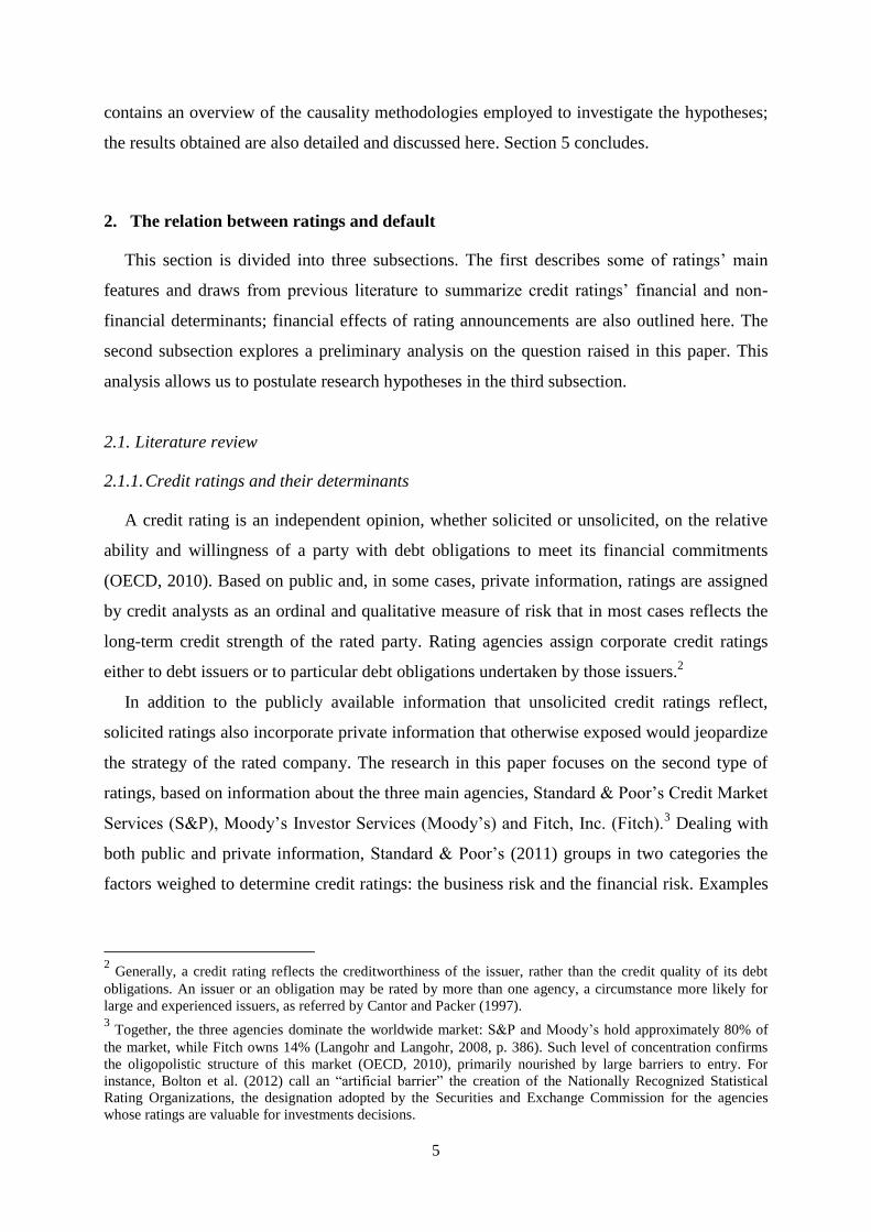
21
IGSG announcements. This seems to suggest that, by transmitting worse news, deeper
downgrades exacerbate the likely effects on credit default. Note that SGSG14 announcements
take place whenever the prior rating level is already a speculative grade. Thus, if SGSG14
announcements determine the probability of default, a prior speculative rating level also
contributes to such probability.
Table 4: Credit default prediction with SGSG14 announcements
This table shows estimates for equations (1) and (2) with SGSG14 announcements. Values reported
derive from logistic regressions of credit default on the firms’ financial and market prior information,
as well as its rating information. In equation (1) such information is given by a dummy denoting
SGSG14 announcements ( ), whereas in equation (2) it is given by a continuous variable denoting the
magnitude of rating changes in these announcements ( ). Both rating variables relate to the 3 years
prior to .
Equation (1) Equation (2)
Estimates z-value p-value Estimates z-value p-value
Intercept -11.7043 -51.69 0.000 -11.8904 -52.75 0.000
Size 0.4297 20.46 0.000 0.4649 22.64 0.000
TDLM 1.3151 6.10 0.000 1.4855 6.92 0.000
Sigma 46.3960 30.21 0.000 46.0403 30.18 0.000
NIATM -5.0045 -20.71 0.000 -5.0627 -21.03 0.000
LTAT 3.2453 23.99 0.000 3.3119 24.58 0.000
CHATM -2.2545 -4.97 0.000 -2.1092 -4.70 0.000
MB -0.3589 -7.35 0.000 -0.3599 -7.38 0.000
1.8674 20.44 0.000
0.4881 16.77 0.000
Pseudo-R2 0.4581 0.4500
Likelihood Ratio 6,932.96 (p-value = 0.000) 6,809.90 (p-value = 0.000)
Observations 109,767
2.3. Research hypotheses
The results in Tables 3 and 4 suggest that downgrades to speculative levels relate to an
abnormal increase in the rated firm’s probability of default. We consider as normal a firm’s
probability of default that reflects exclusively the intrinsic economic context of that firm, such
as its financial performance and demographic characteristics. Abnormal reactions arise in that
probability whenever exogenous factors, such as external opinions transmitted by research
analysts in general and rating announcements in particular, are significant to the firm’s
probability of default. For example, Campbell et al. (2008) find that stocks with low analyst
coverage reveal stronger financial distress anomaly; however, they do not inform about the

22
effects when analysts deliver negative perspectives. Given the influence of ratings on the
firm’s credibility, we expect that they generate similar effects as those illustrated by Merton
(1968, p. 366) in the bank’s parable. Hence, we define the following hypothesis.
H1: An IGSG announcement generates an overreaction in the firm’s probability of default.
The implications of this hypothesis may be extended. If an IGSG announcement provokes
an abnormal increase in the probability of default, it is highly likely that worse
announcements also affect that probability. Considering the results in Table 4 and in view of
higher debt burden due to worse ratings, we postulate that lower rating levels both prior to
and after the announcement will exacerbate the probability of default. This hypothesis is
consistent with Jorion and Zhang (2007), who find that lower rated firms reveal higher
negative reactions to downgrades, namely in their stock prices. Therefore, we define the next
hypothesis.
H2: Deeper downgrades, given by SGSG14 announcements, cause greater effects on the
firm’s probability of default.
In order to evaluate whether we should accept any of these hypotheses, the study adopts
two well-known causality approaches for the empirical analysis: the propensity score
matching approach and the Heckman treatment effects model. The results follow in Section 4.
3. Data
The empirical investigation in this study derives from a sample of rated and non-rated U.S.
firms. With the objective to get a relevant set of comparable firms, we delimit the universe of
analysis to public non-financial and non-public administration firms (all SIC codes not
comprised between 6000-6999 and not over 9000), the vast majority currently listed or having
been listed in NYSE, AMEX or NASDAQ. The time frame considered spans from 1990 to
2012, a length similar to other studies on financial distress; for example, both Altman (1968)
and Hillegeist et al. (2004) analyse 20 years. Retrieving data from different sources, we build
subsamples for ratings, for several measures of financial and economic performance, and for
credit defaults.
Concerning sources of credit ratings information, the paper uses data from Bloomberg’s
report on Fitch, Moody’s and S&P credit ratings (RATC: Company Credit Rating Changes),
as well as from the databases of S&P and Moody’s. Rating types selected are those that focus
on long term obligations, namely: Moody’s Issuer Rating; S&P’s Issuer Credit Rating and

23
Long Term Local Issuer Credit; Fitch’s Long Term Issuer Default Rating and Long Term
Local Currency Issuer Default.
The CRSP and COMPUSTAT databases are the sources of information respectively for the
firms’ market information and the firms’ financials, relative to the period from 1990 to 2011.
As in Dichev and Piotroski (2001), we exclude cases not covered by COMPUSTAT,
considered as small and marginal firms. In order to avoid disturbances from outliers, all
financial and market variables are winsorized to the 5th
and 95th
percentiles of their
distributions. Relatively to cases with missing values for any financial variable, we set the
omitted value to the respective subsample (default vs. non-default) average for that variable.
Information on corporate defaults from 1991 to 2012 comes from Bloomberg’s report on
corporate actions (CACT: Capital Change; Bankruptcy Filing), CRSP’s delisting code 574,
COMPUSTAT’s inactivation code 02, UCLA - LoPucki Bankruptcy Research Database, from
S&P’s database and from Moody’s Default and Recovery Database. Credit ratings are another
source of information on defaults.
As detailed below, we get a database of 109,767 firm-years, with a default rate of 1.29%
and with 31,072 ratings.
3.1. Ratings
Among the particulars regarding quantitative analyses of credit ratings, we generally find
the need to convert an ordinal and qualitative scale into a numeric scale. This study draws
from previous literature (e.g., Jorion and Zhang, 2007; Güttler and Wahrenburg, 2007), and
from the numeric correspondence generally accepted by regulators for the different long-term
obligations rating scales to define a conversion of rating levels into scores. Table 5 exhibits
this conversion, with the majority of the reference definitions based on the terminology used
by Fitch (2011) and, where applicable, by Moody’s (2012) and S&P.14
The numerical or sign
modifier attached to some ratings adds granularity to the scales, further discriminating the risk
level inside each rating’s main category.
According to Table 5, the higher is the score the greater is the risk. Classes that explicitly
refer to a possible event of default are all scored 22. For example, beyond a rating level
14
http://www.standardandpoors.com/ratings/articles/en/us/?articleType=HTML&assetID=1245335682757
(accessed in August 2012).
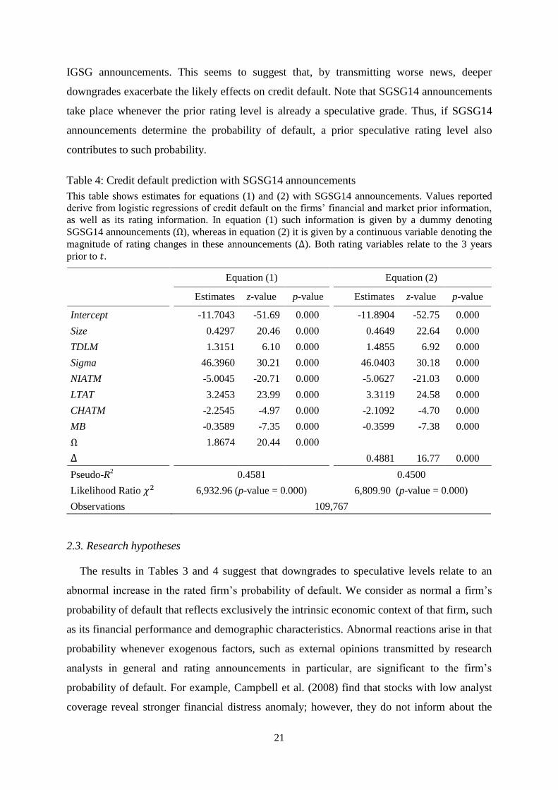
24
denoting obligations in default, a score equal to 22 includes both RD (Fitch) and SD (S&P),
which stand for restrictive and selective default.15
Table 5: Rating scales of different agencies
This table shows the correspondence between the rating scales of Moody’s, S&P and Fitch. A score
for each rating level is added.
Moody’s S&P Fitch Score Reference definitions
Investment grade
Aaa AAA 1 Highest credit quality
Aa1, Aa2, Aa3 AA+, AA, AA- 2, 3, 4 Very high credit quality
A1, A2, A3 A+, A, A- 5, 6, 7 High credit quality
Baa1, Baa2, Baa3 BBB+, BBB, BBB- 8, 9, 10 Good credit quality
Speculative grade
Ba1, Ba2, Ba3 BB+, BB, BB- 11, 12, 13 Speculative grade
B1, B2, B3 B+, B, B- 14, 15, 16 Highly speculative
Caa1, Caa2, Caa3 CCC+, CCC, CCC- 17, 18, 19 Substantial credit risk
- CC 20 Very high levels of credit risk
- C 21 Exceptionally high levels of credit risk
Ca -
22
Obligations likely in, or very near, default
- SD RD Selective / Restrictive default
C D Obligations in default
If an issuer is rated more than once by the same rating agency on the same month, a typical
event whenever distinct long term obligations are rated, we select only the worst rating.
Similarly, within the last 30 days, if a rating agency announced more than once the same
rating for an issuer, we use that rating only once. Likewise, downgrades to default are also
kept out from the ratings subsample, given that, when it occurs, a credit default instantly
becomes a fact known by all investors concerned. As these downgrades do not bring new
information to the market, they are deemed not relevant as potential causes of default. Note,
however, that downgrades to default are sources of information on defaults and will be treated
as such in our subsample of defaults. Applying all previous criteria, we select 31,072 relevant
announcements for analysis. For each firm-year, the rating information is computed for the
previous 3 years, given that ratings aim to reflect long term credit risk, and that we want to
gauge their long term effects.
15
Restrictive and selective defaults stand for defaults not generalized to all debt obligations of the rated firm.

25
3.2. Defaults
A corporate credit default is considered here as an event in which firms are unable to fulfil
their debt obligations. In particular, similarly to the specifications adopted by Fitch, Moody’s
and S&P, this definition includes a bankruptcy event (Chapter 7 and Chapter 11), a failure to
timely pay a debt obligation, or any sort of debt restructuring not foreseen in the initial credit
agreement. This implies the exclusion of technical defaults.
Besides the previous data sources of defaults, we use credit ratings as a source of
information on defaults. Thus, credit ratings that explicitly state that a default event already
occurred, despite their differences in the level of severity, are classified as default and feed the
information on corporate defaults. This is the case of rating D or RD published by Fitch, C
and Ca published by Moody’s, and D or SD published by S&P. As some firms defaulted more
than once, we select the first event observed as reference.
We remove from the sample all defaults without any financial information in the three
years preceding the default event. The same applies to observations for the years following a
default; once a default is observed, all subsequent information is considered as not significant
for the purpose of the investigation.
3.3. Summary statistics
Following the application of the above selection criteria, we obtain a database with a total
of 11,215 firms, 9,799 of which without any default during the period selected and 1,416 with
at least one default. Using a hazard modelling approach, as in Shumway (2001), we also
classify all firms that defaulted as non-defaults in the years that precede the respective default
event. The final sample is thus composed by 109,767 firm-years, and consequently the
corresponding default rate for the whole period is 1.29%.16
We identify 2,536 firms (12,328 firm-years) with at least one rating during the period of
analysis, of which 580 defaulted at least once. This shows a proportionately higher fraction of
rated firms in the subsample of defaults. Considering the prior 3-year rating information for
each firm-year, the number of ratings expands to 58,564 announcements of which 3,332
belong to the subsample of defaults, and the remaining referring to non-defaulted firms in
subsequent years. Table 6 summarizes the distribution of the sample of firms, with the
number of ratings in terms of firm-years between brackets.
16
Note that our estimate of the default rate should be lower than the true value, due to the restriction we apply to
firms that defaulted more than once.

26
Table 6: Distribution of the sample of firm-years and ratings
This table reports the aggregate distribution of the sample of firm-years and ratings (in brackets) used
for analysis, according to cases with or without default and cases with or without ratings. The sample
analyzed includes observations from 1990 to 2012.
Defaults Non-defaults
With rating 580 (3,322) 11,748 (55,242)
Without rating 836 96,603
Table 7 shows the yearly distribution of the previous information; the year of analysis for
each firm is denoted as the reference year. In the case of defaulted firms, the reference year
represents the time when credit default occurs.
Table 7: Yearly distribution of the sample
This table displays the distribution of data along the sample period. Per reference year, it includes the
number of defaulted and non-defaulted firms, the rate of default, the number of rating announcements
in the 3-year period prior to the reference year, respectively for defaulted and non-defaulted firms, as
well as the 3-year prior IGSG-type of rating announcements.
Reference
year
Firms Number of announcements IGSG announcements
Subsample
of defaults
Subsample of
non-defaults
Rate of
default Subsample
of defaults
Subsample of
non-defaults Total % of ratings
1991 57 4,693 1.2% 23 713 13 1.7%
1992 53 4,912 1.1% 13 1,221 15 1.2%
1993 63 5,277 1.2% 28 1,608 29 1.8%
1994 37 5,577 0.7% 14 1,596 26 1.6%
1995 49 5,876 0.8% 35 1,861 40 2.1%
1996 39 6,542 0.6% 24 2,053 38 1.8%
1997 42 6,621 0.6% 37 2,247 39 1.7%
1998 77 6,411 1.2% 92 2,674 52 1.9%
1999 100 6,413 1.5% 249 3,407 65 1.7%
2000 131 5,992 2.1% 347 2,862 67 2.0%
2001 195 5,505 3.4% 644 3,658 103 2.3%
2002 124 5,065 2.4% 414 3,414 103 2.6%
2003 71 4,816 1.5% 227 3,655 111 2.8%
2004 35 4,651 0.7% 117 3,389 84 2.4%
2005 29 4,533 0.6% 90 3,324 80 2.3%
2006 32 4,378 0.7% 76 3,422 80 2.3%
2007 31 4,073 0.8% 71 2,826 53 1.8%
2008 68 3,824 1.7% 259 2,703 65 2.2%
2009 125 3,625 3.3% 457 3,025 77 2.1%
2010 31 3,435 0.9% 52 2,872 54 1.8%
2011 21 3,203 0.7% 33 2,602 46 1.7%
2012 6 2,929 0.2% 20 110 1 0.8%
The information concerning the number of ratings indicates announcements observed in
the 3-year period prior to the reference year. As expected, there is a higher prevalence of

27
defaults and of the default rate around major U.S. economic crises, such as the sharp
economic slowdown of 2001 and the pronounced recession of 2009. In other words, the
overall risk of default is, as expected, significantly influenced by macroeconomic conditions.
The last two columns of Table 7 represent the number of IGSG-type of announcements
observed in the 3-year period prior to the year of reference and the respective proportion of
the number of ratings observed in the same period. As in the case of the rate of default, we
find that the percentage of IGSG announcements rises when the state of the economy goes
through significant declines. It seems interesting to note as well in Figure 3 that, in addition to
triggering a higher intensity of rating announcements, economic downturns originate a higher
preponderance of ratings observed in the subsample of defaults.
Figure 3: Yearly distribution of the prior 3-year announcements
From a univariate analysis perspective, the relation between the rate of default and the
previously observed type of rating announcements, reflected in Table 8, is derived from the
31,072 announcements selected initially.17
The table tells us that rates of default tend to be
higher when ratings announcements are harsher: in general, upgrades are followed by lower
rates of default than downgrades, and within the latter the worse rating changes precede the
highest rates of default. For example, the rate of default corresponding to an IGSG
announcement exceeds an impressive 12% within three years from the date of announcement,
specifically when the inherent downgrade is by two or more classes.
17
By focusing on rating announcements, Table 8 provides different information relative to what credit rating
agencies typically disclose, namely the relation between the rating level (which may have been announced way
before) and the subsequently observed rate of default.
0
900
1,800
2,700
3,600
4,500
0%
3%
6%
9%
12%
15%
Nr. of Ratings % IGSG (3Y) % Ratings (subset of defaults)
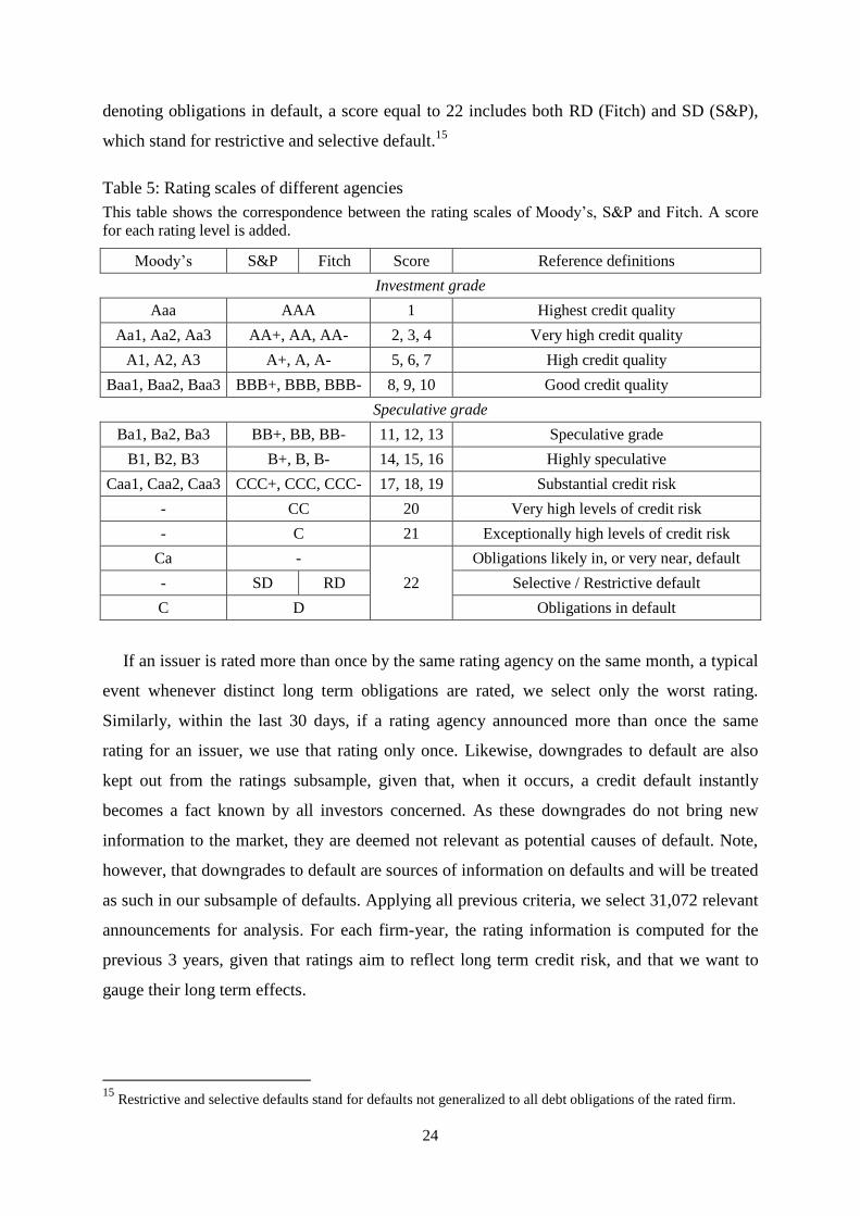
28
Table 8: Rate of default per type of prior rating announcements
This table shows how the rate of default evolves according to the type of rating announcement, the
initial and final rating levels and the magnitude of the rating change. The 1-year and 3-year time
frames following the announcements are selected for analysis. The last column contains the number of
ratings per type of announcement.
Type of rating announcement Rate of default
Total … within 1 year … within 3 years
Downgrades
• IG to IG 1 class 0.93% 2.18% 1,926
> 1 class 1.55% 3.26% 582
• IG to SG 1 class 3.17% 9.80% 347
> 1 class 6.95% 12.43% 547
• SG to SG 1 class 16.40% 31.44% 3,524
> 1 class 36.94% 47.57% 2,098
Upgrades
• IG to IG 0.06% 0.98% 1,641
• SG to IG 0.44% 1.56% 1,604
• SG to SG 2.24% 10.00% 5,391
Unchanged & New ratings n.a. 13,412
In line with the results in Subsection 2.2, Table 8 also confirms that deeper downgrades
precede much stronger rates of default. Although such information could be regarded as an
indication of the predictive power of ratings, the fact is that it also does not preclude the
possibility of an influence of ratings on the variable they are trying to predict.
Complementary, if we position ourselves in each reference year and look at prior rating
information, a substantiation of differences between defaulted and non-defaulted firms
emerges, as shown in Table 9. As in Güttler and Wahrenburg (2007), the evidence shows that,
the closer is the default event, the worse is correspondingly the firm’s average rating.
Moreover, when compared to the subsample of non-defaults, defaults constantly reveal lower
ratings (higher scores) and a slightly higher number of announcements. In addition, although
both type of firms denote a continuous downtrend of ratings (i.e. higher consecutive scores)
along the last three years, in the case of defaulted firms that trend is much more remarkable.
In order to get a better understanding of the financial performance within the two
subsamples, we also compute the averages of some financial ratios and variables in the year
prior to the reference year in each subsample. The selection of such variables derives from
previous literature on financial distress forecasting, in particular Campbell et al. (2008), as
well as the accounting-type and market variables already specified in Table 1.

29
Table 9: Prior rating information
This table reports the average for selected rating information observed in the 3-year period prior to the
reference year, which in the case of defaults corresponds to the year of default. The results of the
defaulted firms are compared to those of non-defaulted firms.
Defaults Non-defaults
Rating in t-1 15.18 10.65
Rating in t-2 14.45 10.43
Rating in t-3 13.83 10.14
Nr. of ratings in t-1 2.44 2.05
Nr. of ratings in t-2 2.12 2.07
Nr. of ratings in t-3 2.29 2.13
Hence, using annual data and in line with definitions presented in Section 2.1, we compute
the following variables: Interest Coverage (IC), Operating Margin (OM), Long Term Debt
Leverage (LTDL), Total Debt Leverage (TDL), Total Debt divided by Market Value of Assets
(TDLM). We analyze as well other variables previously mentioned, namely Operating Income
Before Depreciation divided by Total Assets (OAT), natural logarithm of Total Assets (Size),
natural logarithm of Total Debt (Debt), firm’s stock beta (Beta), annual standard deviation of
the firm’s daily stock return (Sigma), and the natural logarithm of the firm’s stock price at the
close of each year’s last trading session (Price). Following Campbell et al. (2008), this study
also examines Net Income divided by Total Assets (NIAT), Net Income divided by the Market
Value of Assets (NIATM), Total Liabilities divided by Total Assets (LTAT), Total Liabilities
divided by the Market Value of Assets (LTATM), Cash and Short Term Investments divided
by the Market Value of Assets (CHTAM), and Market to Book Ratio (MB).
Table 10 summarizes the results obtained. As expected, the table complements the results
shown in Table 2. On average, defaulted firms reveal high leverage (greater LTDL, TDL,
TDLM, LTAT and LTATM) and poorer profitability (smaller IC, OM, OAT, NIAT and
NIATM). Such firms also signal lower market valuation (smaller Price and MB), as well as
higher risk, as reflected in their stock’s return volatility (higher Sigma). Comparing the
subsamples of rated and non-rated firms, one can see that firms in the first subsample have
higher size, debt and systematic risk, as measured by their Beta. Besides, rated firms have
higher leverage and their profitability is greater too.
Remarkably, weak profitability as an indicator that anticipates credit default has a much
more subtle difference in the subsample of ratings when compared to the subsample without
ratings. For example, the IC of defaulted non-rated firms is considerably lower than the one in
defaulted rated firms, the latter being inclusively positive. The higher values of OM and OAT

30
in the defaulted rated firms, when compared to the non-defaulted non-rated firms, are even
more striking. This suggests that less profitable firms are not as much prone to solicit credit
ratings, which is in line with findings from Poon and Chan (2010). As for leverage of
defaulted firms, ratios for the subsample of ratings always exceed levels of firms without
ratings, except in the case of LTAT. With a larger debt burden, it seems thus natural that rated
firms are more exposed to increases in the firm’s cost of funding.
Table 10: Financial indicators
This table reports within the different subsamples the average for each financial variable observed in
the year prior to the reference year. Variables are selected in line with Table 1, as well as additional
covariates tested in Campbell et al. (2008) to predict financial distress.
Defaults Non-defaults
Rated Non-rated Rated Non-rated
IC 0.4850 -4.1486 7.7716 6.4165
OM -0.0264 -0.3164 0.1550 -0.1583
LTDL 0.5217 0.2344 0.3161 0.1374
TDL 0.6762 0.4618 0.3610 0.2055
TDLM 0.4912 0.3235 0.2370 0.1389
OAT 0.0367 -0.1597 0.1337 0.0131
Size 6.5382 4.4017 7.4642 4.2554
Debt 6.0568 3.3952 6.2947 2.2169
Beta 0.9430 0.7165 0.9969 0.7688
Sigma 0.0653 0.0827 0.0294 0.0446
Price 0.9844 0.1880 2.9944 1.8153
NIAT -0.1713 -0.4040 0.0237 -0.0887
NIATM -0.1519 -0.2358 0.0082 -0.0325
LTAT 0.9805 0.9654 0.6608 0.4821
LTATM 0.7551 0.6637 0.4407 0.3169
CHATM 0.0568 0.0670 0.0573 0.1088
MB 1.3187 1.6766 1.7381 2.1926
4. Causality analysis
4.1. Literature review of causality methods
4.1.1. Propensity score matching
We can look at a Type- announcement as the “treatment” that a number of firms have to
tackle, and hypothesize that upcoming events of credit default ( ) are among the
outcomes generated by such treatment. Let if a firm has a Type- announcement, and
otherwise. ( ) denotes the expectation of default in each situation; ( ) is the

31
expected level of default related to the announcement and ( ) is the expected level of
default related to its absence.
To compare the factual and counterfactual outcomes, we would need to know the average
treatment effect at the population level.18
Such effect corresponds to the difference in
expected default of firms with a Type- announcement (treated cases) relative to a scenario
where they had not been rated as such (untreated). Formally, as discussed in Imbens (2004),
the average treatment effect is given by ( ); this measure requires that, for each
firm, we were able to observe simultaneously mutually exclusive events. As parallel universes
do not exist, we cannot observe at the same time a firm with and without a Type-
announcement. Thus, we compute instead the average treatment effect of the announcement
only on the subgroup of cases with that treatment (the treated cases), as
( ) ( ) ( ) (4)
In our case, ATT is the average effect of the Type- announcement computed on those firms
that actually had such announcement. As the counterfactual for firms with a Type-
announcements, i.e. ( ), is not observed, it should be estimated by an adequate
method, after which we may estimate ATT.
A way to estimate ATT lies in experimental evaluation, based in a random assignment to
treatment. However, due to limitations inherent to observational studies, where treatment
selection is often determined by subject characteristics, it is not always feasible to use
randomness compliant with this method. Therefore, Rosenbaum and Rubin (1983) propose an
alternative solution for non-experimental data: the propensity score matching (PSM).
The utilization of PSM techniques abounds in different fields of investigation dealing with
causality problems. For example, Dehejia and Wahba (2002) use PSM to investigate the
expected effect of a job training program on individuals’ earnings. Also based on PSM,
Gilligan and Hoddinott (2007) analyse data from Ethiopia to confirm the benefits of an
emergency food aid in terms of welfare, access to food, and food security for many
households after the peak of the drought in 2002. In the medical literature, Williamson et al.
(2011) apply PSM to estimate the effect of maternal choice to give breast milk on the infant’s
consequent neurodevelopment. Another example of PSM, applied to psychology, is in
McCormick et al. (2013), who evaluate the effect of the teacher-child relationship in
18
As before, the factual of downgrades denote what effectively happened to firms with downgrades, while the
counterfactual means what would have happened to the same firms if such downgrades did not occur.

32
kindergarten on the children’s later academic math and reading achievement. Many more
examples could be presented, revealing the widespread acceptance of PSM.
When applied to the problem under analysis in this paper, PSM finds firms without a Type-
announcement with similar characteristics to those with such announcement; this mitigates
the previous potential selection bias. Instead of looking at each observable characteristic or
covariate separately, something that ultimately turns out to be unmanageable, the information
for similarity comparison is captured by one single metric: the propensity score.
Hence, the propensity score provides the conditional probability of a firm receiving
announcements of Type , given a set of observed covariates that identify each firm.
Formally, this score is defined as
( ) ( ) (5)
According to Rosenbaum and Rubin (1983), treatment assignment is strongly ignorable
and identical treated and untreated cases can be unbiasedly matched based on the propensity
score alone, if two main assumptions hold. The first is a conditional independence
assumption, also called the unconfoundedness assumption. It states that, after controlling for
the set of covariates , treatment assignment (e.g., the announcement) produces similar
outcomes as a random process, i.e.
( ) (6)
In our study, this statistical independence implies that a Type- announcement depends only
on the covariates that influence it. The rationale behind this assumption is that, in the presence
of enough information on the factors determining the type of rating announcement, we can
remove the correlation between ( ) and by conditioning on . As demonstrated in the
seminal paper of Rosenbaum and Rubin (1983), the correlation can also be removed by
conditioning on ( )
( ) ( ) (7)
The second assumption is a common support condition that admits a positive probability
for both treatment and non-treatment, as represented by
( ) (8)
This assumption is essential to ensure that we find matches for and in the region
of common support, which implies that a balancing property needs to hold; i.e., firms with the
same propensity score have similar distributions of covariates, regardless of the
33
announcement status. Firms with and without a Type- announcement may therefore be
matched according to their propensity score. As a consequence, we need to identify cases
whose predicted probability of treatment (the announcement) is similar, i.e. ( )
( ). This means the matching procedure and the estimates of the propensity score
need to balance the distributions of covariates between both groups, rather than being
concerned with the most accurate estimate for the true propensity score. Hence, considering
(8), ATT remains valid only for those firms with announcements which are comparable to the
firms without announcements, i.e. where common support remains.
As long as the previous assumptions hold and taking into account (7), we may estimate
ATT using the unconditional effect over the predicted probability of having a Type-
announcement. The announcement effect for firm is
[ ( ) ( )]
∑ ( )
(9)
where ( ) is the weight assigned to matched firm to aggregate outcomes in the control
group. [ ( ) ( )] is the counterfactual for firm , which can be estimated
as a weighted average of outcomes in the control group ( ). Aggregating (9) for all
firms with the announcement, we obtain an estimator of (4) by averaging the effect, as in
Heckman et al. (1998)
∑ [ ∑ ( )
]
(10)
Note that, albeit the balancing property may have been reached, as ( ) is a continuous
variable there is a null probability of obtaining two cases with exactly the same propensity
score. To overcome this problem, we need to apply appropriate matching methods and choose
accordingly the weights to apply. This study estimates equation (10) using the Nearest-
Neighbor Matching (NNM), one of the most popular matching methods. For each treated case
in the sample, NNM selects the untreated observation with the closest propensity score; this
observation is given a weight equal to one, and all others are set to zero. Using this procedure,
we estimate the counterfactual treatment outcome.

34
In order to apply the propensity scoring methodology and to estimate ATT, we follow the
process proposed by Abadie et al. (2004). The variables determining credit ratings, as outlined
in Subsection 2.1, are then selected as potential covariates for the propensity to have a Type-
announcement. Here, we allow for the advantages of including only those variables that
determine treatment assignment, as highlighted by Austin et al. (2007).
4.1.2. The Heckman treatment effects
Heckman (2008) underlines the potential benefits of “explicitly formulated econometric
models” to causal inference, given their virtue in providing insights about the dependencies
between the distinct variables involved. In equation (1), we use an econometric approach to
measure the effects that Type- announcements might have on credit default, considering as
exogenous the treatment dummy variable . Yet, given that such rating announcements may
depend on common factors determining credit default, it seems appropriate to take care of an
endogeneity issue in .
In order to deal with such issue, and as an alternative to the causality approach in PSM, we
now use the evaluation of treatment effectiveness as proposed by Maddala (1983, p. 120); this
is an extension to the sample selection model developed by Heckman (1978, 1979). This
model, often called as the Heckman treatment effects approach, or Heckit model, is useful
when we want to control for the conceivable endogeneity of the decision to have credit
ratings. An example of the application of the Heckit model to the context of credit ratings is in
An and Chan (2008), who investigate the effects of credit ratings on the pricing of initial
public offerings.
Based on the Heckit model, a selection equation embedding a probit model is defined as
{1 iff i
0
0 otherwise
(11)
is a latent endogenous variable related with , the binary variable that indicates treatment
(i.e. rating announcement), represents, as before, the vector of exogenous variables
determining the selection of firm for treatment in time period , and are regression
coefficients; is an error term assumed normal. The selection equation and the probit model
interact as ( ) ( ), where ( ) is the distribution function of a standard
normal random variable.
The outcome equation is
35
( )
( )
(12)
, , and have the same meaning as in equation (1). is additionally assumed to
be normally distributed, as well as ( ) and ( ).
Equation (12) is expressed by a functional form which may be nonlinear, as in equation
(1), or linear. We adopt the response or outcome function in the original framework of the
Heckit model, which is linear. Actually, when the outcome is a probability, a nonlinear
function such as the logit or probit functions seems more appropriate, but its use is nontrivial,
as discussed in Angrist (2001) and in Freedman and Sekhon (2010). As we are mostly
concerned with the variation in the probability of default due to Type- announcements,
instead of the true value of the probability, a linear function may not be inappropriate; the
variation in this case is directly provided by . Also, when using a linear function, we may
interpret the estimate of as a valuation of ATT, thus providing a comparison between both
models.
Finally, a special concern must be paid to the correlation coefficient between error terms of
equation (11) and (12), denoted by . If is statistically different from zero, and
consequently are correlated with . Then, the direct estimation of equation (12) will
generate an endogeneity problem, materialized in biased and inconsistent estimators. The bias
may be overthrown estimating simultaneously with the outcome variable , using either a
two-step consistent estimator or maximum likelihood.
4.2. Results of the propensity score matching approach
In order to predict the occurrence of Type- announcements, specifically IGSG and
SGSG14 announcements, we use indicators of profitability, leverage, size and market.
According to the through-the-cycle perspective of ratings, in line with previous research (e.g.,
Blume et al., 1998), and consistent with the dependent variable (defined as a 3-year event),
we compute the 3-year averages of financial and market indicators as potential covariates.
The prefix Av is added to each covariate to denote the respective 3-year average prior to the
reference year. As the dependent variable is binary (announcement vs. absence of
announcement), we apply a logistic regression instead of ordered logit or ordered probit

36
approaches.19
Denoting as the 3-year average of each covariate ( ),
equation (12) provides the propensity of a Type- announcement in firm and time period
( )
[ ( ∑ )]
(13)
and are parameters and is a residual variable.
Note that all observations, rated and unrated, are inputs to estimate the regression;
therefore, the probability of a type announcement reflects the simultaneous occurrence of
two events: the firm is rated and has a type- announcement. The first event is actually a
requirement for the second, since a firm cannot have a Type- announcement without being
rated. Table 11 exhibits the results.
Table 11: Prediction of Type- announcements
This table reports the estimates of two logistic regressions that predict Type- announcements,
respectively IGSG and SGSG14, based on the firms’ financial and market prior information. The
covariates, denoted with prefix Av for each variable, refer to the 3-year average of that variable.
IGSG announcements SGSG14 announcements
Estimates z-value p-value Estimates z-value p-value
Intercept -11.6276 -43.78 0.000 -8.1028 -56.17 0.000
AvLTDL 1.6197 8.92 0.000 5.4635 42.33 0.000
AvSize 1.1762 37.86 0.000 0.5421 31.46 0.000
AvBeta 0.1586 2.17 0.030 0.4980 8.90 0.000
AvNIATM -3.5296 -6.55 0.000 -4.6610 -13.56 0.000
AvMB -0.7892 -13.05 0.000 -0.7088 -16.16 0.000
Pseudo-R2 0.3024 0.2698
Likelihood Ratio 4,110.05 (p-value = 0.000) 5,645.70 (p-value = 0.000)
Observations 109,767
The AUROC in the case of IGSG announcements is 0.9323, higher than the 0.9086 we get
in the regression for SGSG14 announcements; this is consistent with the difference in the
Pseudo-R2 for both regressions. In any circumstance, these indicators imply, once again, high
accuracy and statistical relevance. The results suggest as well a low multicolinearity level,
given all near zero p-values, the correlation between covariates mostly well below 0.5, and in
view of signs of parameters generally in line with expectations.
19
In spite of probit or logit being the most common econometric techniques used, there are exceptions. For
example, Kisgen (2006) uses ordinary least squares to regress credit ratings on a few covariates. However, an
overall agreement on the inappropriateness of the least squares method and of methods that ignore the ordinal
nature of bond ratings has already been reported in Kamstra et al. (2001).

37
We may conclude that IGSG events are more likely in firms with higher long term debt
leverage, size and market model beta. Conversely, IGSG events are less probable in firms
with higher market value valuation and profitability, here given by net income divided by
total assets. Except in the case of size, these results are consistent with the expected influence
reported in previous literature, as shown in Table 1. In what concerns size, the findings
suggest a negative influence on ratings, which results in a greater likelihood of downgrades of
IGSG type in larger firms. This is somewhat contrary to the findings in Kisgen (2006).
Besides potential differences in the samples, another conceivable explanation for
dissimilarities in results lies in the fact that our model predicts the occurrence of two events,
which include the likelihood of being rated, in addition to the type of rating assigned. Indeed,
Table 7 confirms the expectation that largest companies are more likely to be rated. Three of
the previous types of covariates are also common to the regression that predicts credit default:
size of firms, profitability and market value. Although leverage belongs to both regressions,
we measure it differently in each of them. TDLM and LTAT adjust better to forecast credit
default, whereas AvLTDL is better to predict IGSG and SGSG14 announcements.
In relation to SGSG14 announcements, it is noteworthy to underline that both leverage and
market risk have significantly higher marginal effects when compared to the results obtained
for IGSG announcements; the same applies to the respective z-values. Such results suggest a
higher influence of these variables on deeper downgrades.
Based on the previous selection of covariates, we apply the propensity score methodology
and estimate the average treatment effect on the treated, ATT. As described in Subsection
4.1.1, we select the nearest-neighbor matching method, whence the estimates of ATT,
reported in Table 12, are obtained. This table also contains the associated standard errors,
fundamental to know if the estimated average treatment effect is significantly different from
zero; the estimation of standard errors use bootstrapping.20
The extremely low p-values
confirm that both announcements are statistically significant and positive. This means that
downgrades equal to (or worse than) a change from investment grade to speculative grade
have causality effects on the probability of default, confirming hypothesis H1.
20
This estimation method of standard errors consists in drawing new samples with replacement from the
existing sample, from where the model and propensity scores are re-estimated several times; the standard error is
derived from the different results obtained.

38
Table 12: ATT estimations when IGSG or SGSG14 announcements are selected as treatment
This table reports estimates of average treatment effect on the treated, when the treatment variable is
the occurrence of IGSG or SGSG14 announcements. Selecting as covariates of propensity score the
variables in Table 11, the estimation of ATT derives from nearest-neighbor matching methods.
Estimate Standard Error z-value p-value
ATT (IGSG) 0.0306 0.0072 4.23 0.000
ATT (SGSG14) 0.1213 0.0084 14.51 0.000
We observe that when downgrades are IGSG-type, ATT equals 3.06%. This is the
estimated effect in the 1-year probability of default due to a downgrade of IGSG-type.
Interestingly, this estimate is quite near the 3.59% shown in Subsection 2.2.4, when we
estimated a credit default prediction model with IGSG announcements. In contrast, the effect
of SGSG14 announcements, equal to 12.13%, is way above the value detected in the case of
IGSG, although nonetheless below the 16.59% derived in Subsection 2.2.5. The much larger
effect in the case of SGSG14 is relevant to corroborate hypothesis H2. Therefore, we show
that greater effects on the firm’s probability of default emerge as a result of deeper
downgrades, given by SGSG14 announcements. As these announcements denote prior ratings
which are already speculative grade, the influence of SGSG14 also means that low prior
rating levels contribute to the probability of default.
In order to confirm the consistency of these results, we extend the analysis to the Heckman
treatment effects approach.
4.3. Results of the Heckman treatment effects approach
Estimating a Heckit model requires that we first define the variables both in the selection
equation (11) and in the regression equation (12). Given the high accuracy revealed by our
previous estimations, we use variables selected for estimating credit default (Table 2) and
credit announcements (Table 11); the maximum likelihood method allows us to estimate
regressions parameters. As in the case of the propensity score matching, we estimate effects
of both type of announcements, IGSG and SGSG14. However, when estimating the effects of
IGSG announcements using the Heckit model, the outcomes show a statistically significant
estimate of ; in a test of correlation between error terms, we do not accept the null
hypothesis, H0: 0 (p-value equal to 0.007). This means that this estimation method does
not fully remove the threat of endogeneity bias in equation (1). Anyhow, the value of , equal
to 0.0332, is actually quite low, suggesting therefore that the level of correlation between the
two error terms, and , is similarly low. Hence, as this model adds little to findings from

39
previous methodologies, we do not consider the Heckit model’s results in the case of IGSG
announcements.
Outputs from the Heckit model relative to SGSG14 announcements follow in Table 13.
The estimate of indicates once more a negligible value ( -0.002), implying that the risk
of endogeneity bias in equation (1) remains remote. With a p-value of 0.765, H0: 0 is now
accepted, supporting the remoteness of such risk.
Table 13: Treatment effects model estimates for SGSG14 announcements
This table shows estimates of the Heckman treatment effects model, when SGSG14 announcements
are selected as treatment variable. , the endogenous in the selection equation, is simultaneously a
covariate in the regression equation that predicts credit default. The related parameter estimate
indicates the direction of the effect.
Estimate Standard Error z-value p-value
Regression equation ( )
Constant -0.0846 0.0019 -44.79 0.000
Size 0.0061 0.0002 32.11 0.000
TDLM 0.0334 0.0029 11.33 0.000
Sigma 0.9232 0.0197 46.93 0.000
NIATM -0.1186 0.0036 -33.14 0.000
LTAT 0.0365 0.0015 24.26 0.000
CHATM -0.0085 0.0036 -2.33 0.020
MB -0.0001 0.0003 -0.26 0.793
0.1335 0.0028 48.04 0.000
Selection equation ( )
Constant -4.0181 0.0640 -62.74 0.000
AvLTDL 2.5224 0.0603 41.81 0.000
AvSize 0.2452 0.0079 30.96 0.000
AvBeta 0.2532 0.0264 9.58 0.000
AvNIATM -2.2951 0.1641 -13.98 0.000
AvMB -0.2895 0.0187 -15.50 0.000
-0.0020 0.0066
0.1063 0.0002
-0.0002 0.0007
Wald 13,010.48 (p-value = 0.000)
Observations 109,767
Likelihood Ratio test of independent equations ( = 0): (1) = 0.09 ( p-value = 0.765)
In what concerns the direction of influence of each covariate, the signs of parameters are
consistent with economic intuition, though MB reveals a low z-value. Of particular interest to
the analysis in this study, is the estimate of the parameter associated to . As mentioned at the
end of Subsection 4.1, the regression equation of the outcome variable (in our case, the

40
probability of default ) in the Heckit model is linear. Hence, , the parameter associated to
, gives the direct effect of the occurrence of an SGSG14 announcement, which compares to
the ATT. The respective estimate is positive and statistically significant at the 5% significance
level. The effect is therefore estimated in 13.35%, a value between the estimate derived from
the ATT and the direct estimation of credit default, accounting for SGSG14 announcements.
4.4. Interpretation and implication
Despite using different methods to estimate the potential effects caused by negative ratings
announcements on subsequent credit defaults, we detect relatively similar results when
selecting two types of announcements (Table 14). All estimates of these potential effects are
relevant at the 1% significance level, except in the case of the Heckman treatment effects
method applied to IGSG announcements.
Notwithstanding the relative similarity of results, a careful interpretation is recommended.
These results suggest that some negative rating announcements cause an increase in the rated
firm’s default. We interpret this effect as being a reflection of undermined investors’
confidence, following the negative news conveyed by ratings. Moreover, the worse is the
information in ratings announcements, in particular when deeper downgrades are disclosed,
the more affected is investors’ confidence; therefore, the stronger is the impact on the issuer
financial performance and on its risk of default.
Table 14: Estimated effects caused by IGSG and SGSG14 announcements on credit default
This table summarizes the results achieved using the methodologies discussed in Sections 5 and 6.
Estimation method IGSG effects SGSG14 effects
Credit default prediction model 3.59% 16.59%
Propensity score matching 3.06% 12.13%
Heckman treatment effects n.a. * 13.35%
* Non-significant estimate at the 5% significance level.
However, these results should not be seen as a red light for issuers looking to be rated.
Indeed, credit ratings remain doubtless a very powerful and essential market instrument for
most firms to obtain funding at a relatively low cost. What our findings really seem to suggest
is that, prior to soliciting ratings, issuers should first evaluate the extent to which they are
economically sound enough to avoid future deeper downgrades. The trade-off for some firms
is between an immediate potential benefit of lower cost of funding and a probably higher cost
of financial distress in the future. On the other hand, our findings imply that, when

41
announcing deeper downgrades, rating agencies should be fully aware of the respective
potential negative feedback effects.
Finally, these results also bring a powerful insight for credit default prediction models,
namely in what concerns the covariates of those models. In fact, due to the causal effects of
rating announcements, specifically when they convey negative news, the inclusion of rating
information as a covariate of such models is expected to add to the accuracy of prediction
already given by the firm's intrinsic details. Löffler and Maurer (2011) reinforce such
perspective, by finding that current rating is a significant explanatory variable in their default
prediction model.
5. Summary and concluding remarks
Credit ratings convey information to the markets. In what concerns a firm’s risk of default,
this paper confirms that some negative rating announcements are relevant enough to generate
additional pressures for a default in the rated firm's obligations. The pervasive effects that
such announcements seem to generate reinforce the perception that, to a certain extent, rating
agencies are powerful enough to determine the unfolding outcomes of the markets. In the
words of Langohr and Langohr (2008, p. 473), they are considered “among the more powerful
and less understood financial institutions on the planet”.
Benefiting from an extensive database of rating announcements and supported by
complementary methodologies for causality analysis, the evidence in this paper suggests that
rating downgrades from an investment grade to a speculative grade have a non-trivial effect in
the firm’s probability of default. The effect is substantially amplified when levels of rating
prior and after announcement are lower, namely when we observe downgrades for an already
speculative grade level to a level at best highly speculative. Consistent with these findings, the
probability of default also seems to worsen with the magnitude of rating downgrade.
By confirming effects of rating announcements on a firm’s future performance, we
corroborate and mainly provide an explanation for the finding in Löffler and Maurer (2011),
that ratings provide valuable information for default prediction. Conceivable extensions of
this line of research remain in the analysis of other rating-related information as covariates of
credit default models, as well as in the inclusion of information regarding the state of the
business cycle. For example, relative to the latter, we might conjecture that the potential
causal effects of negative credit ratings on credit default will be heightened particularly under
recession periods, when firms are financially more vulnerable. This is particularly relevant if

42
we consider that reputation cycles in ratings relate, to some degree, with business cycles
fluctuations.
References
Abadie, Alberto, David Drukker, Jane Herr, and Guido Imbens, 2004, Implementing
Matching Estimators for Average Treatment Effects in Stata, The Stata Journal 4, 290-
311.
Altman, Edward, 1968, Financial Ratios, Discriminant Analysis and the Prediction of
Corporate Bankruptcy, The Journal of Finance 23, 589-609.
Altman, Edward, and Duen Kao, 1992, The Implications of Corporate Bond Ratings Drift,
Financial Analysts Journal 48, 64-75.
Amato, Jeffery, and Craig Furfine, 2004, Are Credit Ratings Procyclical?, Journal of Banking
and Finance 28, 2641–2677.
An, Heng, and Kam Chan, 2008, Credit Ratings and IPO Pricing, Journal of Corporate
Finance 14, 584–595.
Angrist, Joshua, 2001, Estimation of Limited Dependent Variable Models with Dummy
Endogenous Regressors: Simple Strategies for Empirical Practice, Journal of Business and
Economic Statistics 19, 2-28.
Austin, Peter, Paul Grootendorst, and Geoffrey Anderson, 2007, A Comparison of the Ability
of Different Propensity Score Models to Balance Measured Variables between Treated and
Untreated Subjects: A Monte Carlo study, Statistics in Medicine 26, 734–753.
Bannier, Christina, and Marcel Tyrell, 2006, Modelling the Role of Credit Rating Agencies:
Do They Spark Off a Virtuous Circle?, Working Paper Series: Finance and Accounting
160, Department of Finance, Goethe University Frankfurt am Main.
Bharath, Sreedhar, and Tyler Shumway, 2008, Forecasting default with the Merton distance to
default model, Review of Financial Studies 21, 1339–1369.
Black, Fischer, and Myron Scholes, 1973, The Pricing of Options and Corporate Liabilities,
Journal of Political Economy 81, 637-654.
Blume, Marshall, Felix Lim, and A. Craig MacKinlay, 1998, The Declining Credit Quality of
U.S. Corporate Debt: Myth or Reality?, The Journal of Finance 53, 1389-1413.
Bolton, Patrick, Xavier Freixas, and Joel Shapiro, 2012, The Credit Ratings Game, The
Journal of Finance 67, 85-111.
Campbell, John, Jens Hilscher, and Jan Szilagyi, 2008, In Search of Distress Risk, The
Journal of Finance 63, 2899-2939.
Cantor, Richard, and Frank Packer, 1997, Differences of Opinion and Selection Bias in the
Credit Rating Industry, Journal of Banking and Finance 21, 1395-1417.
Chava, Sudheer, and Robert Jarrow, 2004, Bankruptcy prediction with industry effects,
Review of Finance 8, 537–569.
Daniels, Kenneth, and Malene Jensen, 2005, The Effect of Credit Ratings on Credit Default
Swap Spreads and Credit Spreads, The Journal of Fixed Income 15, 16-33.
43
Dehejia, Rajeev, and Sadek Wahba, 2002, Propensity Score-Matching Methods for
Nonexperimental Causal Studies, The Review of Economics and Statistics 84, 151–161.
Dichev, Ilia, and Joseph Piotroski, 2001, The Long-Run Stock Returns Following Bond
Ratings Changes, The Journal of Finance 56, 173-203.
Ederington, Louis, and Jeremy Goh, 1998, Bond Rating Agencies and Stock Analysts: Who
Knows What When?, Journal of Financial and Quantitative Analysis 33, 569-585.
Fitch, 2011, Definitions of Ratings and Other Forms of Opinion, Fitch Ratings, December.
Fons, Jerome, 2002, Understanding Moody’s Corporate Bond Ratings And Rating Process,
Special Comment, Moody’s Investors Service, New York.
Freedman, David, and Jasjeet Sekhon, 2010, Endogeneity in Probit Response Models,
Political Analysis 18, 138-150.
Fulop, Andras, 2006, Feedback Effects of Rating Downgrades, ESSEC Working Papers DR
06016.
Giesecke, Kay, Francis Longstaff, Stephen Schaefer, and Ilya Strebulaev, 2011, Corporate
Bond Default Risk: A 150-year Perspective, Journal of Financial Economics 102, 233–
250.
Gilligan, Daniel, and John Hoddinott, 2007, Is There Persistence in the Impact of Emergency
Food Aid? Evidence on Consumption, Food Security, and Assets in Rural Ethiopia,
American Journal of Agricultural Economics 89, 225–242.
Gonzalez, Fernando, F. Hass, R. Johannes, M. Persson, L. Toledo, R. Violi, M. Wieland, and
C. Zins, 2004, Market Dynamics Associated with Credit Ratings: A Literature Review,
European Central Bank Occasional Paper Series 16.
Graham, John, and Campbell Harvey, 2001, The Theory and Practice of Corporate Finance:
Evidence from the Field, Journal of Financial Economics 60, 187-243.
Güttler, André, and Mark Wahrenburg, 2007, The Adjustment of Credit Ratings in Advance
of Defaults, Journal of Banking and Finance 31, 751–767.
Hand, John, Robert Holthausen, and Richard Leftwich, 1992, The Effect of Bond Rating
Agency Announcements on Bond and Stock Prices, The Journal of Finance 47, 733-752.
Heckman, James, 1978, Dummy Endogenous Variables in a Simultaneous Equation System,
Econometrica 46, 931-959.
Heckman, James, 1979, Sample Selection Bias as a Specification Error, Econometrica 47,
153-161.
Heckman, James, 2008, Econometric Causality, International Statistical Review 76, 1-27.
Heckman, James, Hidehiko Ichimura, and Petra Todd, 1998, Matching as an Econometric
Evaluation Estimator, Review of Economic Studies 65, 261-294.
Hillegeist, Stephen, Elizabeth Keating, Donald Cram, and Kyle Lundstedt, 2004, Assessing
the Probability of Bankruptcy, Review of Accounting Studies 9, 5-34.
Hilscher, Jens, and Mungo Wilson, 2011, Credit Ratings and Credit Risk, Working Paper 31,
Brandeis University, Department of Economics and International Business School.
Holland, Paul, 1986, Statistics and Causal Inference, Journal of the American Statistical
Association 81, 945-960.

44
Holthausen, Robert, and Richard Leftwich, 1986, The Effect of Bond Rating Changes on
Common Stock Prices, Journal of Financial Economics 17, 57-89.
Hu, Yu-Chiang, and Jake Ansell, 2007, Retail Default Prediction by Using Sequential
Minimal Optimization Technique, Journal of Forecasting 28, 651-666.
Hull, John, Mirela Predescu, and Alan White, 2004, The Relationship Between Credit Default
Swap Spread, Bond Yields, and Credit Rating Announcements, Journal of Banking and
Finance 28, 2789–2811.
Imbens, Guido, 2004, Nonparametric Estimation of Average Treatment Effects Under
Exogeneity: A Review, The Review of Economics and Statistics 86, 4–29.
Jorion, Philippe, and Gaiyan Zhang, 2007, Information Effects of Bond Rating Changes: The
Role of the Rating Prior to the Announcement, The Journal of Fixed Income 16, 45–59.
Jorion, Philippe, Charles Shi, and Sanjian Zhang, 2009, Tightening Credit Standards: The
Role of Accounting Quality, Review of Accounting Studies 14, 123-160.
Jorion, Philippe, Zhu Liu, and Charles Shi, 2005, Informational Effects of Regulation FD:
Evidence from Rating Agencies, Journal of Financial Economics 76, 309-330.
Kamstra, Mark, Peter Kennedy, and Teck-Kin Suan, 2001, Combining Bond Rating Forecasts
Using Logit, The Financial Review 37, 75–96.
Kisgen, Darren, 2006, Credit Ratings and Capital Structure, The Journal of Finance 61, 1035-
1072.
Kliger, Doron, and Oded Sarig, 2000, The Information Value of Bond Ratings, The Journal of
Finance 55, 2879-2902.
Kuhner, Christoph, 2001, Financial Rating Agencies: Are They Credible? – Insights into the
Reporting Incentives of Rating Agencies in Times of Enhanced Systemic Risk,
Schmalenbach Business Review 53, 2-26.
Lando, David, and Torben Skødeberg, 2002, Analyzing Rating Transitions and Rating Drift
with Continuous Observations, Journal of Banking and Finance 26, 423-444.
Langohr, Herwig, and Patricia Langohr, 2008, The Rating Agencies and their Credit Ratings:
What They Are, How They Work and Why They Are Relevant, John Wiley & Sons.
Löffler, Gunter, and Alina Maurer, 2011, Incorporating the Dynamics of Leverage into
Default Prediction, Journal of Banking and Finance 35, 3351-3361.
Maddala, Gangadharrao, 1983, Limited-Dependent and Qualitative Variables in
Econometrics, Cambridge, UK, Cambridge University Press.
Maffett, Mark, Edward Owens, and Anand Srinivasan, 2013, Default Prediction Around the
World: The Effect of Constraints on Pessimistic Trading, Working Paper.
McCormick, Meghan, Erin O'Connor, Elise Cappella, and Sandee McClowry, 2013, Teacher–
child Relationships and Academic Achievement: A Multilevel Propensity Score Model
Approach, Journal of School Psychology 51, 611–624.
Merton, Robert C., 1974, On the Pricing of Corporate Debt: The Risk Structure of Interest
Rates, Journal of Finance 29, 449-470.
Merton, Robert K., 1968, Social Theory and Social Structure, The Free Press, Macmillan
Publishing Co., Inc.

45
Micu, Marian, Eli Remolona, and Philip Wooldridge, 2006, The Price Impact of Rating
Announcements: Which Announcements Matter?, BIS Working Papers 207.
Moody’s, 2012, Rating Symbols and Definitions, Moody’s Investors Service, April.
Norden, Lars, and Martin Weber, 2004, Informational Efficiency of Credit Default Swap and
Stock Markets: The Impact of Credit Rating Announcements, Journal of Banking and
Finance 28, 2813-2843.
OECD, 2010, Competition and Credit Rating Agencies, Hearing on Competition and Credit
Rating Agencies held in the Competition Committee meeting on 16 June 2010 (accessed at
http://www.oecd.org/dataoecd/28/51/46825342.pdf in September, 2011).
Ohlson, James, 1980, Financial Ratios and the Probabilistic Prediction of Bankruptcy,
Journal of Accounting Research 18, 109-131.
Poon, Winnie, and Kam Chan, 2010, Solicited and Unsolicited Credit Ratings: A Global
Perspective, ADBI Working Paper 244, Tokyo: Asian Development Bank Institute.
Rosenbaum, Paul, and Donald Rubin, 1983, The Central Role of the Propensity Score in
Observational Studies for Causal Effects, Biometrika 70, 41-55.
Shumway, Tyler, 2001, Forecasting Bankruptcy More Efficiently: A Simple Hazard Model,
Journal of Business 74, 101–124.
Standard & Poor’s, 2011, Guide to Credit Rating Essentials, Standard & Poor’s Financial
Services.
Steiner, Manfred, and Volker Heinke, 2001, Event Study Concerning International Bond
Price Effects on Credit Rating Actions, International Journal of Finance and Economics 6,
139–157.
Stumpp, Pamela, 2001, The Unintended Consequences of Rating Triggers, Special Comment,
Moody’s Investors Service, New York.
Williamson, Elizabeth, Ruth Morley, Alan Lucas, and James Carpenter, 2012, Propensity
Scores: From Naïve Enthusiasm to Intuitive Understanding, Statistical Methods in Medical
Research 21, 273-293.
Recommended