IPS Chapter 6
© 2012 W.H. Freeman and Company
6.1: Estimating with Confidence
6.2: Tests of Significance
6.3: Use and Abuse of Tests
6.4: Power and Inference as a Decision
Introduction to Inference

Objectives
6.1 Estimating with confidence
Statistical confidence
Confidence intervals
Confidence interval for a population mean
How confidence intervals behave
Choosing the sample size

Overview of Inference
Methods for drawing conclusions about a population from sample data are called statistical inference
Methods Confidence Intervals - estimating a value of a population parameter Tests of significance - assess evidence for a claim about a population
Inference is appropriate when data are produced by either a random sample or a randomized experiment
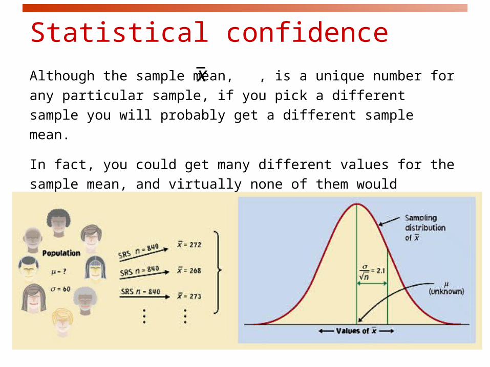
Statistical confidenceAlthough the sample mean, , is a unique number for any particular
sample, if you pick a different sample you will probably get a different
sample mean.
In fact, you could get many different values for the sample mean, and
virtually none of them would actually equal the true population mean, .
x
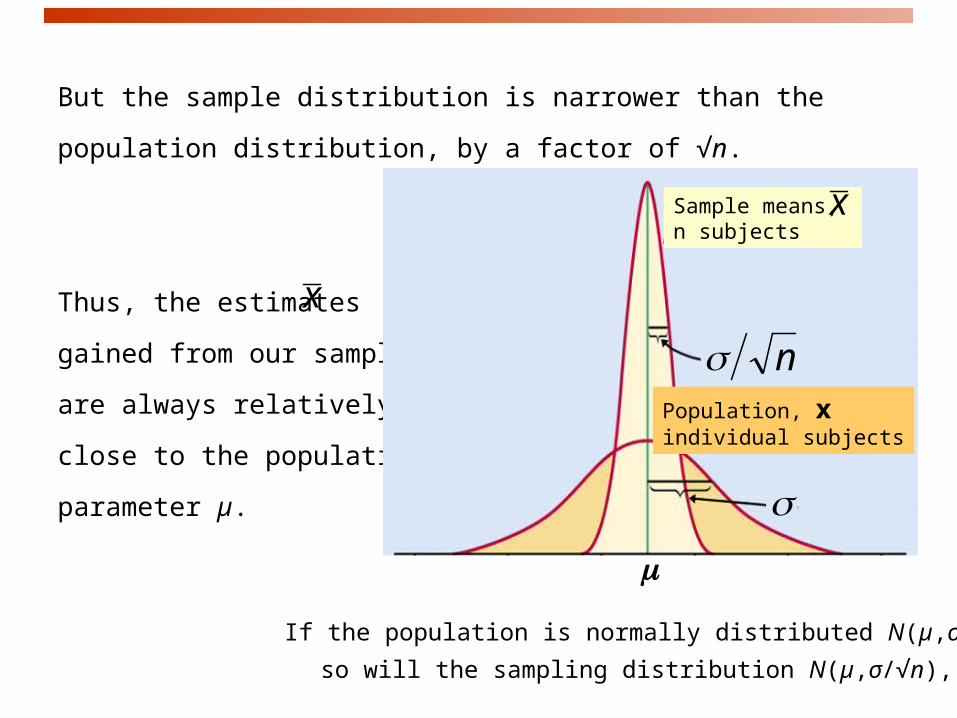
But the sample distribution is narrower than the population distribution,
by a factor of √n.
Thus, the estimates
gained from our samples
are always relatively
close to the population
parameter µ.
nSample means,n subjects
n
Population, xindividual subjects
x
x
If the population is normally distributed N(µ,σ),
so will the sampling distribution N(µ,σ/√n),

Red dot: mean valueof individual sample
95% of all sample means will
be within roughly 2 standard
deviations (2*/√n) of the
population parameter
Distances are symmetrical
which implies that the
population parameter
must be within roughly 2
standard deviations from
the sample average , in
95% of all samples.
This reasoning is the essence of statistical inference.
n
x

The weight of single eggs of the brown variety is normally distributed N(65 g,5 g).Think of a carton of 12 brown eggs as an SRS of size 12.
.
You buy a carton of 12 white eggs instead. The box weighs 770 g.
The average egg weight from that SRS is thus = 64.2 g.
Knowing that the standard deviation of egg weight is 5 g, what
can you infer about the mean µ of the white egg population?
We are 95% confident that the population mean µ is between
64.2 g ± 2.88 g, or roughly within ± 2/√n of .
population sample
What is the distribution of the sample means ?
Normal (mean , standard deviation /√n) = N(65 g,1.44 g).
Find the middle 95% of the sample means distribution.
Roughly ± 2 standard deviations from the mean, or 65g ± 2.88g.
x
x
x

Confidence intervalsThe confidence interval is a range of values with an associated
probability or confidence level C. The probability quantifies the
chance that the interval contains the true population parameter.
± 4.2 is a 95% confidence interval for the population parameter .
This equation says that in 95% of the cases, the actual value of will be within 4.2 units of the value of .
x
x

Implications
We don’t need to take a lot of
random samples to “rebuild” the
sampling distribution and find
at its center.
n
n
Sample
Population
All we need is one SRS of
size n and rely on the
properties of the sample
means distribution to infer
the population mean .

Reworded
With 95% confidence, we can say
that µ should be within roughly 2
standard deviations (2*/√n) from
our sample mean .
In 95% of all possible samples of
this size n, µ will indeed fall in our
confidence interval.
In only 5% of samples would be
farther from µ.
n
x
x
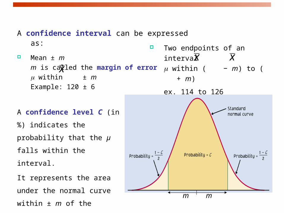
A confidence interval can be expressed as:
Mean ± m
m is called the margin of error
within ± m
Example: 120 ± 6
Two endpoints of an interval
within ( − m) to ( + m)
ex. 114 to 126
A confidence level C (in %)
indicates the probability that the
µ falls within the interval.
It represents the area under the
normal curve within ± m of the
center of the curve.
mm
x
x
x
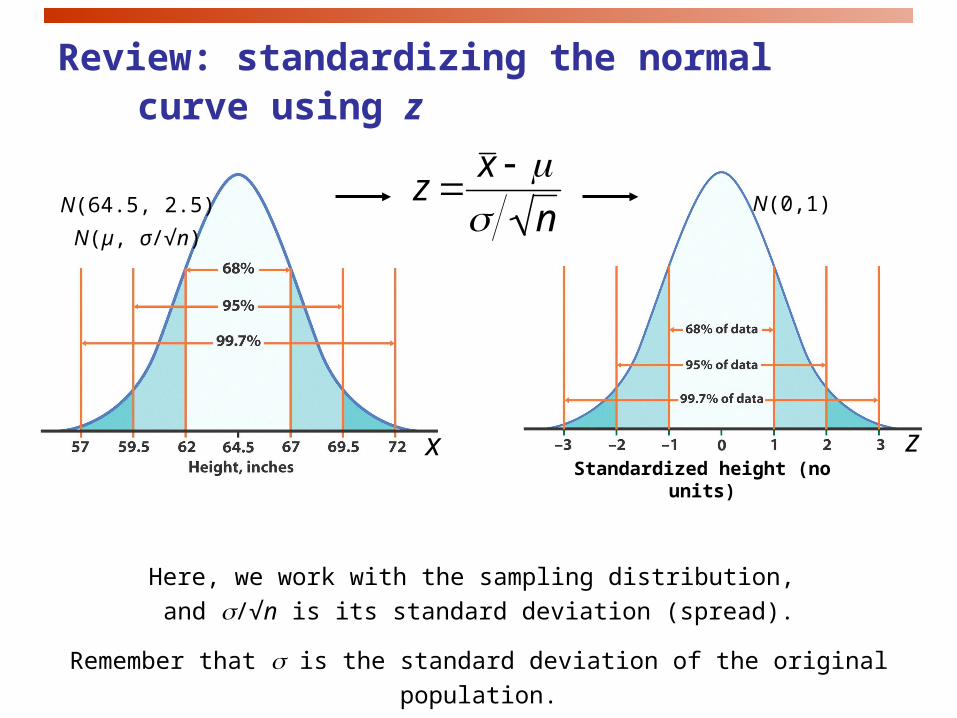
Review: standardizing the normal curve using z
N(0,1)
z
x
N(64.5, 2.5)
N(µ, σ/√n)
Standardized height (no units)
z x n
Here, we work with the sampling distribution,
and /√n is its standard deviation (spread).
Remember that is the standard deviation of the original population.

Confidence intervals contain the population mean in C% of samples.
Different areas under the curve give different confidence levels C.
Example: For an 80% confidence level C, 80% of the normal curve’s
area is contained in the interval.
C
z*−z*
Varying confidence levels
Practical use of z: z*
z* is related to the chosen
confidence level C.
C is the area under the standard
normal curve between −z* and z*.
x z * n
The confidence interval is thus:
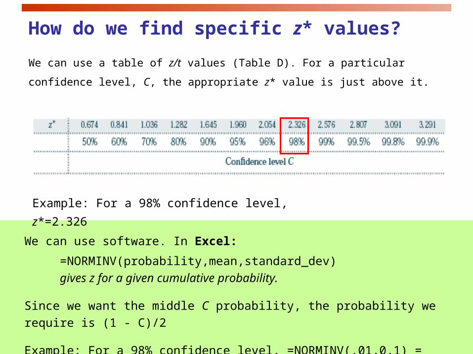
How do we find specific z* values?
We can use a table of z/t values (Table D). For a particular confidence
level, C, the appropriate z* value is just above it.
We can use software. In Excel:
=NORMINV(probability,mean,standard_dev)
gives z for a given cumulative probability.
Since we want the middle C probability, the probability we require is (1 - C)/2
Example: For a 98% confidence level, =NORMINV(.01,0,1) = −2.32635 (= neg. z*)
Example: For a 98% confidence level, z*=2.326

Link between confidence level and margin of errorThe confidence level C determines the value of z* (in table C).
The margin of error also depends on z*.
m z * n
C
z*−z*
m m
Higher confidence C implies a larger
margin of error m (thus less precision
in our estimates).
A lower confidence level C produces a
smaller margin of error m (thus better
precision in our estimates).

Different confidence intervals for the same set of measurements
96% confidence interval for the
true density, z* = 2.054, and write
= 28 ± 2.054(1/√3)
= 28 ± 1.19 x 10⁶
bacteria/ml
70% confidence interval for the
true density, z* = 1.036, and write
= 28 ± 1.036(1/√3)
= 28 ± 0.60 x 10⁶
bacteria/ml
Density of bacteria in solution:
Measurement equipment has standard deviation = 1 * 106 bacteria/ml fluid.
Three measurements: 24, 29, and 31 * 106 bacteria/ml fluid
Mean: = 28 * 106 bacteria/ml. Find the 96% and 70% CI.
nzx
*
nzx
*
x

The margin of error, , gets smaller when z* (and thus the confidence level C) gets smaller σ is smaller n is larger
Properties of Confidence Intervals User chooses the confidence level
Margin of error follows from this choice
z* / n
We want high confidence small margins of error

Impact of sample sizeThe spread in the sampling distribution of the mean is a function of the number of individuals per sample.
The larger the sample size, the smaller the standard deviation (spread) of the sample mean distribution.
But the spread only decreases at a rate equal to √n.
Sample size n
Sta
ndar
d er
ror
⁄ √n

Sample size and experimental design
You may need a certain margin of error (e.g., drug trial, manufacturing
specs). In many cases, the population variability ( is fixed, but we
can choose the number of measurements (n).
So plan ahead what sample size to use to achieve that margin of error.
m z *n
n z *
m
2
Remember, though, that sample size is not always stretchable at will. There are
typically costs and constraints associated with large samples. The best
approach is to use the smallest sample size that can give you useful results.

What sample size for a given margin of error?
Density of bacteria in solution:
Measurement equipment has standard deviation
σ = 1 * 106 bacteria/ml fluid.
How many measurements should you make to obtain a margin of error
of at most 0.5 * 106 bacteria/ml with a confidence level of 95%?
For a 95% confidence interval, z* = 1.96.
n z *
m
2
n 1.96*1
0.5
2
3.922 15.3664
Using only 15 measurements will not be enough to ensure that m is no
more than 0.5 * 106. Therefore, we need at least 16 measurements.

Cautions about using
Data must be a SRS from the population.
Formula is not correct for other sampling designs.
Inference cannot rescue badly produced data.
Confidence intervals are not resistant to outliers.
If n is small (<15) and the population is not normal, the true confidence level will be different from C.
The standard deviation of the population must be known.
The margin of error in a confidence interval covers only random sampling errors!
x z* * / n
Interpretation of Confidence Intervals Conditions under which an inference method is valid are never fully
met in practice. Exploratory data analysis and judgment should be used when deciding whether or not to use a statistical procedure.
Any individual confidence interval either will or will not contain the
true population mean. It is wrong to say that the probability is 95%
that the true mean falls in the confidence interval.
The correct interpretation of a 95% confidence interval is that we are 95% confident that the true mean falls within the interval. The confidence interval was calculated by a method that gives correct results in 95% of all possible samples.
In other words, if many such confidence intervals were constructed, 95% of these intervals would contain the true mean.
Introduction to Inference
6.2 Tests of Significance
© 2012 W.H. Freeman and Company

Objectives
6.2 Tests of significance
The reasoning of significance tests
Stating hypotheses
The P-value
Statistical significance
Tests for a population mean
Confidence intervals to test hypotheses
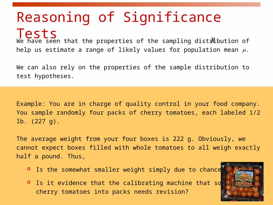
Reasoning of Significance Tests
We have seen that the properties of the sampling distribution of help us
estimate a range of likely values for population mean .
We can also rely on the properties of the sample distribution to test hypotheses.
Example: You are in charge of quality control in your food company. You sample
randomly four packs of cherry tomatoes, each labeled 1/2 lb. (227 g).
The average weight from your four boxes is 222 g. Obviously, we cannot expect
boxes filled with whole tomatoes to all weigh exactly half a pound. Thus,
Is the somewhat smaller weight simply due to chance variation?
Is it evidence that the calibrating machine that sorts
cherry tomatoes into packs needs revision?
x

Stating hypotheses
A test of statistical significance tests a specific hypothesis using
sample data to decide on the validity of the hypothesis.
In statistics, a hypothesis is an assumption or a theory about the
characteristics of one or more variables in one or more populations.
What you want to know: Does the calibrating machine that sorts cherry
tomatoes into packs need revision?
The same question reframed statistically: Is the population mean µ for the
distribution of weights of cherry tomato packages equal to 227 g (i.e., half
a pound)?
The null hypothesis is a very specific statement about a parameter of
the population(s). It is labeled H0.
The alternative hypothesis is a more general statement about a
parameter of the population(s) that is exclusive of the null hypothesis. It
is labeled Ha.
Weight of cherry tomato packs:
H0 : µ = 227 g (µ is the average weight of the population of packs)
Ha : µ ≠ 227 g (µ is either larger or smaller)
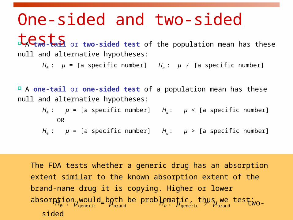
One-sided and two-sided tests A two-tail or two-sided test of the population mean has these null
and alternative hypotheses:
H0 : µ = [a specific number] Ha : µ [a specific number]
A one-tail or one-sided test of a population mean has these null and
alternative hypotheses:
H0 : µ = [a specific number] Ha : µ < [a specific number] OR
H0 : µ = [a specific number] Ha : µ > [a specific number]
The FDA tests whether a generic drug has an absorption extent similar to
the known absorption extent of the brand-name drug it is copying. Higher or
lower absorption would both be problematic, thus we test:
H0 : µgeneric = µbrand Ha : µgeneric µbrand two-sided

How to choose?
What determines the choice of a one-sided versus a two-sided test is
what we know about the problem before we perform a test of statistical
significance.
A health advocacy group tests whether the mean nicotine content of a
brand of cigarettes is greater than the advertised value of 1.4 mg.
Here, the health advocacy group suspects that cigarette manufacturers sell
cigarettes with a nicotine content higher than what they advertise in order to
better addict consumers to their products and maintain revenues.
Thus, this is a one-sided test: H0 : µ = 1.4 mg Ha : µ > 1.4 mg
It is important to make that choice before performing the test or else
you could make a choice of “convenience” or fall into circular logic.

The P-value
The packaging process has a known standard deviation = 5 g.
H0 : µ = 227 g versus Ha : µ ≠ 227 g
The average weight from your four random boxes is 222 g.
What is the probability of drawing a random sample such as yours if H0 is true?
Tests of statistical significance quantify the chance of obtaining a
particular random sample result if the null hypothesis were true. This
quantity is the P-value.
This is a way of assessing the “believability” of the null hypothesis, given
the evidence provided by a random sample.
Interpreting a P-value
Could random variation alone account for the difference between
the null hypothesis and observations from a random sample?
A small P-value implies that random variation due to the sampling
process alone is not likely to account for the observed difference.
With a small p-value we reject H0. The true property of the
population is significantly different from what was stated in H0.
Thus, small P-values are strong evidence AGAINST H0.
But how small is small…?

P = 0.1711
P = 0.2758
P = 0.0892
P = 0.0735
P = 0.01
P = 0.05
When the shaded area becomes very small, the probability of drawing such a
sample at random gets very slim. Oftentimes, a P-value of 0.05 or less is
considered significant: The phenomenon observed is unlikely to be entirely due
to chance event from the random sampling.
Significant P-value
???
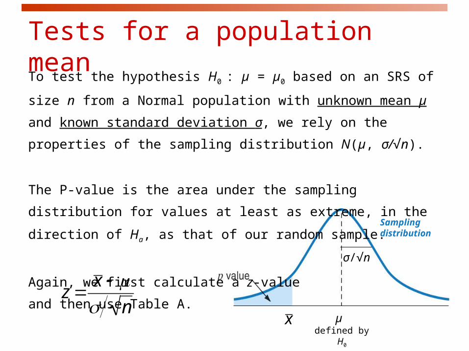
Tests for a population mean
µdefined by H0
x
Sampling distribution
z x n
σ/√n
To test the hypothesis H0 : µ = µ0 based on an SRS of size n from a
Normal population with unknown mean µ and known standard
deviation σ, we rely on the properties of the sampling distribution N(µ,
σ/√n).
The P-value is the area under the sampling distribution for values at
least as extreme, in the direction of Ha, as that of our random sample.
Again, we first calculate a z-value
and then use Table A.

P-value in one-sided and two-sided tests
To calculate the P-value for a two-sided test, use the symmetry of the
normal curve. Find the P-value for a one-sided test and double it.
One-sided
(one-tailed) test
Two-sided
(two-tailed) test

Does the packaging machine need revision?
H0 : µ = 227 g versus Ha : µ ≠ 227 g
What is the probability of drawing a random sample such
as yours if H0 is true?
245
227222
n
xz
From table A, the area under the standard
normal curve to the left of z is 0.0228.
Thus, P-value = 2*0.0228 = 4.56%.
4g5 g222 nx
2.28%2.28%
217 222 227 232 237
Sampling distribution
σ/√n = 2.5 g
µ (H0)2
,z
x
The probability of getting a random
sample average so different from
µ is so low that we reject H0.
The machine does need recalibration.

Steps for Tests of Significance
1. State the null hypotheses Ho and the alternative hypothesis Ha.
2. Calculate value of the test statistic.
3. Determine the P-value for the observed data.
4. State a conclusion.

The significance level:
The significance level, α, is the largest P-value tolerated for rejecting a
true null hypothesis (how much evidence against H0 we require). This
value is decided arbitrarily before conducting the test.
If the P-value is equal to or less than α (P ≤ α), then we reject H0.
If the P-value is greater than α (P > α), then we fail to reject H0.
Does the packaging machine need revision?
Two-sided test. The P-value is 4.56%.
* If α had been set to 5%, then the P-value would be significant.
* If α had been set to 1%, then the P-value would not be significant.
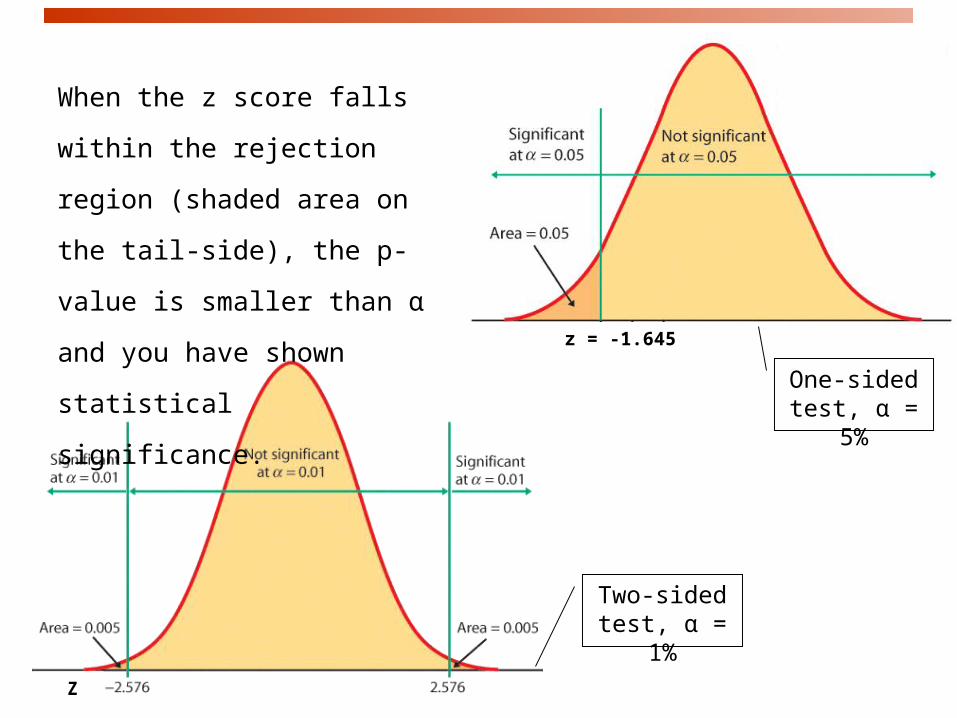
When the z score falls within the
rejection region (shaded area on
the tail-side), the p-value is
smaller than α and you have
shown statistical significance.z = -1.645
Z
One-sided test, α = 5%
Two-sided test, α = 1%

Rejection region for a two-tail test of µ with α = 0.05 (5%)
upper tail probability p 0.25 0.20 0.15 0.10 0.05 0.025 0.02 0.01 0.005 0.0025 0.001 0.0005
(…)
z* 0.674 0.841 1.036 1.282 1.645 1.960 2.054 2.326 2.576 2.807 3.091 3.291 Confidence interval C 50% 60% 70% 80% 90% 95% 96% 98% 99% 99.5% 99.8% 99.9%
A two-sided test means that α is spread
between both tails of the curve, thus:
-A middle area C of 1 − α= 95%, and
-An upper tail area of α/2 = 0.025.
Table C
0.0250.025
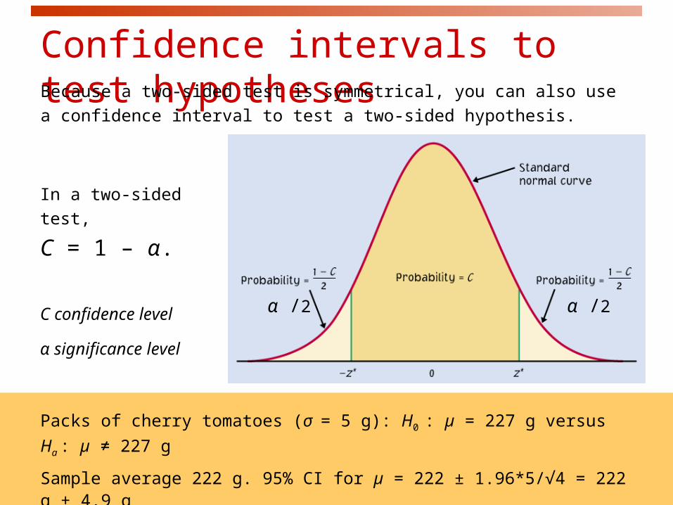
Confidence intervals to test hypothesesBecause a two-sided test is symmetrical, you can also use a
confidence interval to test a two-sided hypothesis.
α /2 α /2
In a two-sided test,
C = 1 – α.
C confidence level
α significance level
Packs of cherry tomatoes (σ= 5 g): H0 : µ = 227 g versus Ha : µ ≠ 227 g
Sample average 222 g. 95% CI for µ = 222 ± 1.96*5/√4 = 222 g ± 4.9 g
227 g does not belong to the 95% CI (217.1 to 226.9 g). Thus, we reject H0.

Ex: Your sample gives a 99% confidence interval of .
With 99% confidence, could samples be from populations with µ = 0.86? µ = 0.85?
x m 0.84 0.0101
99% C.I.
Logic of confidence interval test
x
Cannot rejectH0: = 0.85
Reject H0 : = 0.86
A confidence interval gives a black and white answer: Reject or don't reject H0.
But it also estimates a range of likely values for the true population mean µ.
A P-value quantifies how strong the evidence is against the H0. But if you reject
H0, it doesn’t provide any information about the true population mean µ.

Introduction to Inference
6.3 Use and Abuse of Tests 6.4 Power and Decision
© 2012 W.H. Freeman and Company
Objectives
6.3 Use and abuse of tests
6.4 Power and inference as a decision
Cautions about significance tests
Power of a test
Type I and II errors
Error probabilities
Choosing the significance level α
Factors often considered:
What are the consequences of rejecting the null hypothesis
(e.g., global warming, convicting a person for life with DNA evidence)?
Are you conducting a preliminary study? If so, you may want a larger α so
that you will be less likely to miss an interesting result.
Some conventions:
We typically use the standards of our field of work.
There are no “sharp” cutoffs: e.g., 4.9% versus 5.1 %.
It is the order of magnitude of the P-value that matters: “somewhat
significant,” “significant,” or “very significant.”
Cautions about significance tests

Practical significance
Statistical significance only says whether the effect observed is
likely to be due to chance alone because of random sampling.
Statistical significance may not be practically important. That’s because
statistical significance doesn’t tell you about the magnitude of the
effect, only that there is one.
An effect could be too small to be relevant. And with a large enough
sample size, significance can be reached even for the tiniest effect.
A drug to lower temperature is found to reproducibly lower patient
temperature by 0.4°Celsius (P-value < 0.01). But clinical benefits of
temperature reduction only appear for a 1° decrease or larger.
Don’t ignore lack of significance
Consider this provocative title from the British Medical Journal: “Absence
of evidence is not evidence of absence.”
Having no proof of who committed a murder does not imply that the
murder was not committed.
Indeed, failing to find statistical significance in results is not
rejecting the null hypothesis. This is very different from actually
accepting it. The sample size, for instance, could be too small to
overcome large variability in the population.
When comparing two populations, lack of significance does not imply
that the two samples come from the same population. They could
represent two very distinct populations with similar mathematical
properties.

Interpreting effect size: It’s all about
contextThere is no consensus on how big an effect has to be in order to be
considered meaningful. In some cases, effects that may appear to be
trivial can be very important.
Example: Improving the format of a computerized test reduces the average
response time by about 2 seconds. Although this effect is small, it is
important since this is done millions of times a year. The cumulative time
savings of using the better format is gigantic.
Always think about the context. Try to plot your results, and compare
them with a baseline or results from similar studies.

The power of a test
The power of a test of hypothesis with fixed significance level α is the
probability that the test will reject the null hypothesis when the
alternative is true.
In other words, power is the probability that the data gathered in an
experiment will be sufficient to reject a wrong null hypothesis.
Knowing the power of your test is important:
When designing your experiment: select a sample size large enough to
detect an effect of a magnitude you think is meaningful.
When a test found no significance: Check that your test would have had
enough power to detect an effect of a magnitude you think is meaningful.

Test of hypothesis at significance level α 5%:
H0: µ = 0 versus Ha: µ > 0
Can an exercise program increase bone density? From previous studies, we
assume that σ = 2 for the percent change in bone density and would consider a
percent increase of 1 medically important.
Is 25 subjects a large enough sample for this project?
A significance level of 5% implies a lower tail of 95% and z = 1.645. Thus:
658.0
)25/2(*645.10
)(*
)()(
x
x
nzx
nxz
All sample averages larger than 0.658 will result in rejecting the null hypothesis.

What if the null hypothesis is wrong and the true population mean is 1?
The power against the alternative
µ = 1% is the probability that H0 will
be rejected when in fact µ = 1%. 80.0)855.0(
252
1658.0
)1 when 658.0(
zP
n
xP
xP
We expect that a
sample size of 25
would yield a
power of 80%.
A test power of 80% or more is considered good statistical practice.
Factors affecting power: Size of the effectThe size of the effect is an important factor in determining power. Larger effects are easier to detect.
More conservative significance levels (lower α) yield lower power. Thus, using an α of .01 will result in less power than using an α of .05.
Increasing the sample size decreases the spread of the sampling distribution and therefore increases power. But there is a tradeoff between gain in power and the time and cost of testing a larger sample.
A larger variance σ2 implies a larger spread of the sampling distribution, σ/sqrt(N). Thus, the larger the variance, the lower the power. The variance is in part a property of the population, but it is possible to reduce it to some extent by carefully designing your study.

Ho: µ = 0σ = 10n = 30α = 5%
• Real µ is 3 => power = .5
• Real µ is 5.4 => power = .905
• Real µ is 13.5 => power = 1
http://wise.cgu.edu/power/power_applet.html
red area is
larger differences are easier to detect

Ho: µ = 0σ = 10
Real µ = 5.4α = 5%
• n = 10 => power = .525
• n = 30 => power = .905
• n = 80 => power = .999
larger sample sizes yield greater power

Ho: µ = 0Real µ = 5.4
n = 30α = 5%
• σ is 15 => power = .628
• σ is 10 => power = .905
• σ is 5 => power = 1
smaller variability yields greater power

Type I and II errors
A Type I error is made when we reject the null hypothesis and the
null hypothesis is actually true (incorrectly reject a true H0).
The probability of making a Type I error is the significance level .
A Type II error is made when we fail to reject the null hypothesis
and the null hypothesis is false (incorrectly keep a false H0).
The probability of making a Type II error is labeled .
The power of a test is 1 − .

Running a test of significance is a balancing act between the chance α
of making a Type I error and the chance of making a Type II error.
Reducing α reduces the power of a test and thus increases .
It might be tempting to emphasize greater power (the more the better).
However, with “too much power” trivial effects become highly significant.
A type II error is not definitive since a failure to reject the null hypothesis
does not imply that the null hypothesis is wrong.
The Common Practice of Testing of Hypotheses
1. State Ho and Ha as in a test of significance.
2. Think of the problem as a decision problem, so the probabilities of
Type I and Type II errors are relevant.
3. Consider only tests in which the probability of a Type I error is no
greater than α.
4. Among these tests, select a test that makes the probability of a
Type II error as small as possible.

Alternate Slide
The following slide offers alternate software output data and examples
for this presentation.

Steps for Tests of Significance
1. Assumptions/Conditions
Specify variable, parameter, method of data collection, shape of population.
2. State hypotheses
Null hypothesis Ho and alternative hypothesis Ha.
3. Calculate value of the test statistic
A measure of “difference” between hypothesized value and its estimate.
4. Determine the P-value
Probability, assuming Ho true that the test statistic takes the observed value
or a more extreme value.
5. State the decision and conclusion
Interpret P-value, make decision about Ho.
Recommended