UNIVERSITÀ DEGLI STUDI DI TRIESTE Sede Amministrativa del Dottorato di Ricerca
XVIII CICLO DEL DOTTORATO DI RICERCA IN
GEOFISICA DELLA LITOSFERA E GEODINAMICA
INVERSION OF STRONG MOTION DATA FOR SLIP ON EXTENDED FAULTS: THE CASE OF THE TWO M6.5
ICELAND EARTHQUAKES OF JUNE 2000
DOTTORANDO COORDINATORE DEL COLLEGIO DEI DOCENTI DENIS SANDRON t ':f( CHIAR.MO PROF. RICCARDO PETRINI
UNIVERSITÀ DEGLI STUDI DI TRIESTE
v.; l2XL RELATORE
CHIAR.MO PROF. PETER SUHADOLC
U~ DEG STUDI DI TRIESTE

PRESENTAZIONE
Il problema inverso della sorgente sismica consiste nel tentativo di ricostruire la
distribuzione dello scorrimento sulla superficie della faglia alla sorgente. La
soluzione a questo problema è tutt'altro che banale. E' ben noto che il problema è
instabile e dal punto di vista computazionale questa instabilità è equivalente alla
non unicità della soluzione. Quindi, per ottenere una soluzione definita vi è la
necessità di inserire alcuni vincoli fisici nel processo di sorgente in aggiunta alla
semplice richiesta di riprodurre i dati osservati.
Nella prima parte di questa tesi viene introdotto il problema inverso e lo studio
della sorgente nell'ambito della loro impostazione teorica. Dopo un breve
excursus storico su come si è sviluppato e ha preso corpo negli anni lo studio e la
modellazione della sorgente, vengono presentati i principi meccanici base della
teoria della sorgente di un terremoto tettonico (Cap.2) e l'impostazione del
problema inverso nell'approccio cinematico (Cap.3). La descrizione dinamica
della frattura, seppur fisicamente più adatta, conduce alla formulazione di
problemi con condizioni al contorno nella teoria dell'elasticità che sono
addirittura irrisolvibili nella loro forma generale. La descrizione cinematica in
termini del salto di spostamento sulla superficie della faglia come una funzione
della posizione e del tempo, permette non solo di formulare il problema inverso
ma anche l'esistenza della soluzione. Usando il teorema di rappresentazione lo
spostamento registrato in una stazione sulla superficie della terra può essere
espresso in termini della distribuzione di scorrimento sulla superficie della
faglia. Assumendo che la faglia sia piana e la direzione dello scorrimento
costante, il problema può essere discretizzato, vincolato e ricondotto a un sistema
di equazioni lineari del tipo Ax = b, in cui A è la matrice delle funzioni di Green,

b rappresenta la matrice dei dati reali, e x è l'incognita rappresentata dalla
matrice con la distribuzione di momento sulle celle in cui è suddivisa la faglia.
Per risolvere il sistema lineare abbiamo usato il metodo del simplesso.
Strumento fondamentale nella procedura di calcolo e cuore della procedura di
inversione adottata in questa tesi, il metodo del simplesso viene introdotto
nell'ambito dello studio della programmazione lineare e applicato ad un piccolo
esempio esplicativo (Cap. 4).
Si definiscono come problemi di programmazione lineare tutti quei problemi di
ottimizzazione in cui la funzione obiettivo è lineare e i vincoli sono tutti espressi
da disuguaglianze lineari (ad esempio il vincolo di non negatività delle variabili).
Il Metodo del Simplesso, proposto nel 1947 da G.B.Dantzig, è l'algoritmo di
ottimizzazione più famoso e più utilizzato nelle applicazioni. La strategia seguita
per determinare la soluzione ottima è la seguente: data una soluzione
ammissibile (una scelta qualsiasi di valori che soddisfano i vincoli) se ne
determina un'altra in modo da aumentare, o almeno non diminuire, il
corrispondente valore della funzione obiettivo. In altre parole se abbiamo a
disposizione una soluzione ammissibile essa ci dà un'approssimazione per
difetto del valore ottimo che noi cerchiamo.
Nel nostro caso la funzione obiettivo è rappresentata dal vettore dei residui
(r = b- Ax) che viene minimizzato seguendo la formulazione sviluppata da Das
e Kostrov (Cap. 5).
Buona parte del lavoro è stato quello di adattare alle workstation in ambiente
linux del Dipartimento di Scienze della Terra il pacchetto di programmi software
ii

elaborato proprio per il calcolo dell'inversione di forme d'onda per ottenere lo
scorrimento sismico sulla faglia estesa.
L'applicazione pratica della procedura è stato lo studio dei due terremoti forti
dell'Islanda nel giugno del 2000. I dati sono stati raccolti attraverso la ISESD,
analizzati ed elaborati anche con la collaborazione dell'Università dell'Islanda
soprattutto per quanto riguarda l' orientazione delle stazioni accelerometriche
scelte per l'inversione e non indicate nel database, mentre per la determinazione
dei tempi assoluti di cui non tutte le stazioni dispongono, ci siamo avvalsi di un
precedente lavoro svolto al dipartimento. Dopo una breve descrizione, anche dal
punto di vista geologico, sull'Islanda in generale e sulla SISZ in particolare (Cap.
6), vengono presentati i risultati sia in termini di distribuzione di scorrimento
sulla superficie della faglia sia in termini di confronto tra le forme d'onda reali e
calcolate (Cap. 7) delle inversioni dei due eventi, l'uno del17 Giugno e l'altro del
21 Giugno del 2000. Tutte le inversioni sono state fatte imponendo vincoli fisici
quali la causalità, la positività e il momento prefissato totale.
I risultati migliori sono stati ottenuti usando tutte e tre le componenti dei segnali
e mostrano somiglianze con quelli ottenuti dall'inversione di dati geodetici e
proposti in altri lavori. Per quanto riguarda l'evento del 21 Giugno il massimo
del rilascio di momento sismico è localizzato ad una profondità di circa 5 km,
circa2 km a sud dell'ipocentro e in corrispondenza dell'intersezione della faglia
principale con la faglia coniugata che si estende verso ovest, dove sono state
osservate fratture superficiali. Nella parte più in profondità della faglia si
evidenzia un'incremento del rilascio di momento che segue
approssimativamente la distribuzione degli aftershock. Due ulteriori massimi
sono localizzati in superficie, il più piccolo 4 km a sud dell'ipocentro, il secondo a
2 km a nord dello stesso.
iii

La distribuzione di momento ottenuta invece per l'evento del17 Giugno mostra
come il massimo sia posizionato nella parte centrale della faglia con
un'estensione di circa 8 km in lunghezza e 9 km in profondità. Un secondo
massimo è localizzato più in superficie, circa l km a sud del bordo meridionale
della faglia. Due ulteriori picchi sono ottenuti in prossimità della superficie
vicino al margine settentrionale della faglia il primo, appena a sud del centro
della faglia il secondo.
La validità delle inversioni sarebbe testata meglio se i relativi risultati fossero
paragonati con le reali distribuzioni di scorrimento sulla faglia, ma questo
purtroppo è impossibile per gli eventi naturali. In assenza della possibilità di
confrontare le inversioni con le soluzioni vere, l'unico modo per testare
l'algoritmo è quello di applicarlo a dei dati sintetici ottenuti dalla soluzione del
problema diretto basato sempre sul teorema di rappresentazione (Cap. 8). Questo
approccio ci permette di stimare la risoluzione delle soluzioni ottenute.
Infine per completare lo studio del processo di sorgente è stato fatto uno scenario
dello scuotimento del terreno nella regione in studio (SISZ) utilizzando sia una
distribuzione uniforme di momento sulla faglia sia applicando la distribuzione
stessa ottenuta dalle inversioni (Cap. 9).
iv

In d ex
1. An historical overview of the source modelling......................................... .... . .. .. .. l
2. Theory of tectonic earthquake sources: basic mechanical principles
2.1. Introduction........ ... . . .. . . .. . . . . . . ... . . . .. . . . . ... ... . . . . .. . . . . . . . . . . . . . . . . . . . .. .. ........ .. 9
2.2. The process of shear stress release. .. . . . . . . . . . . .. . . . . . . . . . . . . . . . . .. ... .. . . ................ lO
2.3. The definition of a tectonic earthquake source........... ......... ... ... ............ 13
2.4. Treatment of a discontinuities within a continuous medium................... 14
2.5. Dynamics of a continuous medium, the linear elastic formulation
problem ........................................................................................ 18
3. The inverse problem of earthquake source theory
3.1. Introduction .................................... '. .. . .. .. . .. . . . . . . . . . . . .. . .. . .. . .. ... . ......... 28
3.2. Green-Volterra formula; Green's tensor in linear elastodynamics.............. 29
3.3. Generai solution to the kinematics dislocation problem; formulation of
the inverse problem... ......... ...... ... ............... ... ... ...... .......... ............... 34
4. Linear programming problem and Simplex Algorithm
4.1. Linear programming........................... ............................................ 42
4.2. Fundamental theorem of linear optimization... ........................ .............. 45
4.3. Simplex method fora restricted N ormai Form.. ... . . . . . . . . . . . . . . . . . . . . . ... . . . . . . .... 48
4.4. Example of application of the Simplex procedure . . . . . . . . . . . . . . . . . . . . . . . . . . . . . . ... 51
5. Numerica} solution of the inverse problem
5.1. "Introduction................................................................................. 57
5.2. Inversion for seismic slip rate history and distribution
with stabilizing constraints.... .. ..... .. . ........ . . . . . . . . . . . . . . . . . . . . . . . . . . . . . . . . . . . . .. . ......... 60
5.3. The linear programming approach developed by Das an d Kostrov....... .... 64
I

5.4. Computational considerations ........................................................... 73
6. Outline of the geology of Iceland
6.1. Geologica! an d Geotecnic Settings .. .. .. .. .. .. .. .. .. .. .. .. .. .. .. .. .. .. .. .. .. .. .. .. .. .. .. .. .. . 77
6.2. Bedrock formation................................................................... . . . . . . 78
6.3. Earthquakes.... . . . . . . . . . . . . . . . . . . . . . . . . . . . . . . . . . . . . . . . . . . . . . . . . . . . . . . . . . . . . . . . . . . . . . . . . . . . . . . 80
6.4. The South Iceland Seismic Zone .......................................................... 82
6.5. Short term precursors of the June 17 earthquake................................... 84
6.6. The Icelandic Strong Motion Network................................................ 87
6.7. Pre-processing of the data................................................................. 90
6.8. Crustal structure beneath Iceland ...................................................... 92
6. 9. The structural m o del . . . . . . . . . . . . . . . . . . . . . . . . . . . . . . . . . . . . . . . . . . . . . . . . . . . . . . . . . . . . . . . . . . . . . . 93
7. Source modelling
7.1. Discretization of the source. . . . . . . . . . ... . . . . . . . . . . . . . . . . . . . . . . . . . . . . . . . . . . . . . . . . . . . . . . . . . 96
7.2. Source time function modelling .. .. .. .. .. .. .. .. .. .. .. .. .. .. .. .. .. .. .. .. .. .. .. .. .. .. .. .. . 98
7.3. The Hestvatn-Fault ........................................................................ 100
7.4. 21 June event: summary of the cases treated ......................................... 101
Case1: M1_IDT3 .............................................................................. 103
Case2: M1_IDT5 .............................................................................. 105
Case3: M2 ....................................................................................... 106
Case4: M1_IDT3_3c ............................................................................ 108
Case5: M1_R .................................................................................... 111
Case6: M1_Dip ................................................................................. 117
7.5. The Holt-Fault ....................................................................... _ ......... 119
7.6. 17 June 2000 event ............................................................................ 121
Case1: M1_IDT5_7s ........................................................................... 122
Case2: M1_5s_3c .............................................................................. 123
Case3: M1_3c_R ................................................................................ 125
II

8. A criticai analysis: uncertainties in slip inversion and synthetic test
8.1. Introduction .................................................................................. 129
8.2. Synthetic test .................................................................................. 130
CaseA: Simple fault inversion ............................................................ 131
CaseB: Different slip distribution with J17 parameters ........................... 133
CaseC: Synthetic inversion for J17 Event ............................................. 136
Case D: Adding more data ................................................................ 139
9. Strong ground motion scenarios
9.1. Introduction .................................................................................. 142
9 .2. Parameters to describe strong ground motion ...................................... 143
9 .2. Ground shaking scenario in the SISZ area ............................................ 146
10. Conclusions ....................................................................................... 152
11. References .......................................................................................... 156
III

1. An historical overview of the source
modelling
Seismology is the study of the generation, propagation and recording of elastic
waves in the Earth and of the source that produce them. From a scientific point
of view, an earthquake can be considered as a source of information, the
acquisition of which is the subject of seismological research.
The information contained in seismic waves is of two different kinds: the first is
created during the excitation of waves a t the source of the earthquake; the second
is produced by the structure of the medium during the propagation of waves
from the source to the receiver. Therefore, the interpretation of seismic
observations requires the determination of the velocity structure of the medium
and the determination of the earthquake source parameters. Although these two
problems have been recognized almost simultaneously, their roles in the history
of seismology are different and they have developed in different ways.
The study of earthquake sources is much more difficult than that of the earth's
structure and the investigation of earthquake sources received in the past much
less attention than the investigation of the medium. In fact, determining the
velocity structure of the medium usually requires only kinematic parameters of
seismic waves (travel time for body waves and dispersion curves for surface
w a ves) which can be obtained with relative ease from seismograms and can be
accumulated from many earthquakes for joint processing, being independent of
the source process. Moreover, known artificial sources can be used to investigate
the medium. On the other hand, information on the motions and conditions at an
l

earthquake source, an uncontrolled natura! event, is contained mainly in the
wave's dynamics (waveforms) and is unique for every earthquake. Moreover,
this information is partly, and sometimes totally lost because of distortion by
uncalibrated instruments and propagation effects. To eliminate these effects, the
instrument response and the earth structure must be known beforehand in the
frequency band of interest.
Furthermore, the study of earthquake sources has encountered more serious
difficulties in its theoretical aspects than the study of the earth structure. The
inversion for the earth' s structure is based on the theory of elasticity, the
fundamental principles of which were formulated in the nineteenth century, and
the corresponding mathematical methods were developed mainly in the
nineteenth and early twentieth centuries (the Herglotz-Wiechert formula was
obtained in 1907 and Lamb's problem was solved in 1904). On the other hand,
the attempt to achieve a theoretical understanding of earthquake source
phenomena led to problems that at the beginning of the twentieth century were
impossible not only to solve but even to formulate precisely owing to the absence
of adequate physical concepts for such a problem. In fact, although the concept
that earthquakes are the result of fracture of the earth materia! due to tectonic
stresses, known as the elastic rebound theory (formulated by Reid in 1910), the
basis for analyzing this phenomenon (that is, fracture mechanics), was initiated
by Griffith only in 1921 and started to be developed vigorously only after the
Second World War. Most of the dynamic problems in fracture mechanics proved
to be unsolvable analytically by means of classica! methods. Consequently, it was
necessary to invent specific methods of solution for practically every problem.
Nonetheless, fracture mechanics introduced certain physical concepts and
methods of analysis that formed a framework in which to consider the
2

phenomena of fracture nucleation, propagation and arrest in solid bodies and,
particularly, at the earthquake source.
Investigations of earthquake sources were based on by the work of Reid, who
formulated the theory of elastic rebound based on his study of the effects of the
1906 California earthquake. In 1920s the regularity of the distribution of the signs
of first arrivals of seismic waves was discovered mainly by Japanese
seismologists and the concepì of nodal planes was introduced. Nakano (1923)
formulated the problem of finding the point source in the elastic medium for
which the distribution of signs of first arrivals coincides with those observed for
an earthquake and derived expressions for some dipole sources using the
formulas or displacements due to a point force. This idea proved to be fruitful
and the quantitative study of earthquake sources was so initiated.
The determination of the body-force equivalent source is only half of the
problem, since it is also necessary to relate the characteristics of this equivalent
source to some physical concepts of the real earthquake source, namely, to the
concepts involved in Reid's elastic rebound theory. This is reflected in the term
"fault-plane solution", which denotes the body force equivalent source. Later, by
means of the dynamic Green function, the double-couple model was related to
the final slip distribution on the fault due to an earthquake. With the Green
functions, it is possible to obtain an expression for the components of an elastic
field at any point in terms of the displacement jump distribution and history on
the fault. The simplicity of this representation led to the development of a large
variety of source models. The common feature of all these models is that the
distribution of the displacement jump on the fault surface is assumed arbitrarily
(and in most cases as constant) and it was not clear to what extent the results
depended on the choice of a particular distribution. Essentially, such models
represent a transfer to seismology of the theory of dislocations in an elastic
3

medium developed to describe the behaviour of dislocations in crystals and was
accepted for the sake of simplicity.
It may be more useful physically to specify the stresses acting across the face of a
fault including the effect of friction on the fault p lane.
The crack model (Chinnery, 1969) for an earthquake fault has a stronger physical
basis than the dislocational model but the generallack of adequate data does not
allow one to choose between the crack-with-friction model and the Volterra
dislocation model.
To describe the fracture at an earthquake source as a crack, it is necessary to
know the initial distribution of stresses on the fracture surface before the
earthquake and the laws goveming the fracture propagation and interaction of
the fault faces. Then the distribution of the displacement jump on the fault
becomes one of the unknowns. When this distribution is found, solving for other
quantities reduces to the use of Green' s formula. When describing faults as a
fracture, one assumes some physical laws governing the fracturing and the
extemal action applied to the fault (initial stress). Then the motion along the
fracture and within the surrounding medium is solved for, whereas in
dislocational models, the motion along the fault is assumed. This is equivalent to
the way of describing the motion of a material point: kinematic when its
trajectory is given, and dynamic when the forces acting on this point and the
laws governing its motion are given but the trajectory is unknown. In the case of
fracture, when it is described as a dislocation (displacement jump as a function of
space and time is given, i.e. the trajectories of relative motion of all the initially
adjacent particles ), we will call i t kinematic description, and when i t is described
as a crack, we will call it dynamic. Both descriptions are related to the same
thing, the fracture, but it is clear that the kinematics of fractures is an insufficient
basis for the theory of earthquake sources. In fact the displacement jump across
4

the fault cannot be only kinematically related to the physicallaws governing the
nucleation and propagation of fractures in a continuous medium and to the
physical conditions that produce a particular fracture.
Since the 1960's, the dynamic description of the source has been generally
accepted. With this description some new fundamental parameters of the source
have been introduced into seismology. These parameters, such as stress drop,
average slip and fracture area, have replaced ones like source volume and strain
release, which could not be formalized within the framework of the crack
(fracture) model of the source.
It started to become clear that the investigation of earthquake sources needed a
more realistic basis, namely, the physics of fracture in solid bodies. By this time
the mechanics of brittle fracture, which is concerned with the development of
fractures in solids, was fairly advanced and seemed to be a proper foundation for
earthquake source theory. However a simple transfer of the result obtained in
fracture mechanics to seismology was impossible.
For seismological applications, it was necessary to develop the theory of dynamic
fracture propagation especially for a shear fracture. Thus, there arose a need to
generalize brittle fracture mechanics and to develop a method of solving
dynamic problems for shear fracture propagation.
In geophysics as a whole, forward problems are of minor interest, serving only to
clarify underlying physical phenomena. More important are inverse problems
that require the distribution of materia! parameters an d motions in the earth' s
interior to be determined from surface observation. The inverse problem for the
earthquake source has been formulated as one of reconstructing the
displacement jump distribution and history over the fault surface at the source.
The solvability of this problem was investigated, and two conclusions were
5

reached: motion at the source is uniquely determined from its far-field seismic
radiation (uniquess theorem); it is possible to construct a displacement jump
distribution confined to an arbitrarily small area that produces seismic far-field
radiation arbitrarily dose to the observed one (instability theorem). These
features, common to most inverse problem, imply that this problem cannot be
sol ve d without "a priori" information, in addition to seismic information.
"Since the slip motion is a function of time and two space coordinates, a
complete inversion is extremely difficult. The only practical inversion method is
to describe the kinematics of rupture growth in a fault piane using a small
number of parameters, and then determine those parameters from the
seismograms" (Aki, 1972a). At first glance these considerations are supported by
the instability theorem. However, this theorem implies that, in principles, it is
possible to construct two models with a finite number of parameters having
arbitrarily different values, indistinguishable from one another with arbitrarily
accurate seismic observations. Therefore, the additional constraints that have to
be introduced for the practical solution of the inverse problem cannot be
arbitrary, but they should follow from the physics of the source process. The
latter is most adequately described within the framework of fractures mechanics.
The asymmetric Rayleigh wave radiation pattern from the 1952 Kem County,
California, earthquake initiated the idea that the fracture speed was around the
Rayleigh or shear-wave speed of the medium. A similar fracture speed was
found from surface waves of the great Chilean earthquake. This led to the
commonly accepted assumption that the size of the fracture area at the source is
related to the pulse duration by the factor of Rayleigh or shear-wave velocity.
Aki, 1966 developed a method of determining the seismic moment and
connected it with average slip and the area of fracture at the earthquake source.
Then, from the seismic moment and fault size, the stress drop could be
6

estimateci. This development provides a unique possibility for estimating the
stress conditions in the earth' s interior.
In generai, to obtain a complete description of the earthquake source it is
necessary to determine the slip and stress field on the propagating fault in space
and time. Investigations on the properties of the inverse problem have shown
that this would be difficult, if not impossible. Instead, one can determine some
overall integrai features of the sources (e.g., the stress drop or slip averaged over
the fault or the seismic moment tensor). If the principal axes of the source
moment tensor do not change during an earthquake (i.e., if the direction of
faulting and the direction of slip on the fault do not change), then the time
history of the moment tensor can be split into the time constant seismic moment
tensor an d a function describing its time dependence, the so cali ed "source time
function".
Because of the instability of the inverse problem the study of the forward
problem for particular models of fractures at the source is of considerable
importance. Essentially, solving these problems is the only way to obtain some
insight into the detailed mechanics of the earthquake source, as well as to explain
some of the salient features of observations. In other words the solution of
forward problems provides a tool for understanding rather than for processing
data. In most cases, forward problems cannot be solved analytically. This fact has
given rise to the development of sophisticated numerica! techniques and
computer codes for dynamic crack propagation problems. In the construction of
the mathematical models of earthquake source in the 1960s, quantities like stress
drop and fracture speed were assumed to be uniform over the fault. Of course
seismologist did not actually believe that these quantities were constant in the
earth, and from the earliest days, when Haskell (1964) used a line source
7

propagating at a constant speed to model the seismic radiation from
earthquakes, it was clear that this assumptions were made only for the purpose
of enabling the solution of problems. Current models assume that the fault is
planar, though geologie observations often show large deviation from planarity.
As the quality of the data improves more and more details of the observations
will not be explained by existing models, forcing seismologists to develop new
methods and models to account for such observations.
8

2. The theory of tectonic earthquake sources:
basic mechanical principles
2.1. lntroduction
Even if the intuitive notion of an earthquake source might be clear, its definition
is quite vague. One emphasizes different aspects of this concept when defining
the earthquake source for different applications: the source as a point determined
by the first arrivai of seismic waves, as the region were irreversible deformations
occur during an earthquake, as the region were aftershock hypocenters are
distributed, and so forth.
Let us consider the expression "tectonic earthquake source". It implies that the
source is something different from the earthquake itself. By "earthquake" we
mean the process of vibration of the earth' s surface, or the vibration of the earth' s
medium in generai, or the propagation of seismic waves. In this way the source
is viewed as the source or origin of seismic waves. It is something different from
the materia! of the earth, or the medium, in which the waves propagate. A
tectonic earthquake is an earthquake that is produced by tectonic strain, when
the energy radiated is due to the sudden release of tectonic stresses accumulated
during slowly growing tectonic deformation. Since no potential energy is
associated with nonelastic strain, an earthquake occurs as a result of elastic strain
drop. The total strain in the tectonically active region or in a part of it containing
the earthquake source cannot decrease. Thus, the energy released during an
9

earthquake must be due to the transformation of elastic strain into nonelastic
strain. This transformation may occur slowly, by creep or viscous or plastic flow,
or rapidly, during an earthquake.
The fact that earthquakes occur suddenly implies a local instability of the tectonic
deformation. To be unstable, the earth's materia! should be such that, under
certain conditions, an increase in strain would lead to a decrease in stress (stress
release). The widely accepted belief that stress release is associated with the
formation of fractures is base d on observations of ruptures on the earth' s surface
that accompany earthquakes (faults, dislocations) an d on the observation that
earthquakes are confined mostly to the vicinities of large geologie faults. Deep
earthquakes instead occur at depths that are inaccessible to direct observation.
N onetheless, i t can be shown that even for su eh earthquakes, the process of stress
release must produce fractures. Strictly speaking, only those earthquakes
prod uced by the release of shear stress are t o be considered tectonic ones.
2.2. The process of shear stress release
Let us now consider the process of shear stress release in more detail. Consider a
volume of materia!, say, in the form of a cube small enough to assume that strain
& and tress a are homogeneous within it. For simplicity assume also that the
strain and stress orientations do not change during deformation. Than the state
of this volume can be graphically represented by the stress-strain curve. Let us
assume that, at the beginning of deformation, stress also increases in the volume
(or a t least does not decrease ). Then there will be no earthquake, be cause the
volume will always be in equilibrium with the neighbouring parts of the
medium that produce the strain (curve to the left of point A in fig.2.1.A) If above
lO

some strain &o the stress in the body starts decreasing under further increase of
strain, then instability sets in. In fact, consider the situation at point A in fig.
2.1.A. If the body experiences additional strain 11& the stress in it should fall as
compared with the maximum stress a 0 . It will not counterbalance the action of
the environment, and the strain will increase catastrophically unless the stress in
the cube once again increases with strain (strain hardening). Without strain
hardening, the strain will increase indefinitely. Thus to produce a dynamic event,
the stress strain curve must have a descending part (strain weakening).
l l l i c l 8
"1 -- - - - - -- - --t ---------
A
-
-B c D
Fig. 2.1 A) Unstable stress-strain relation. B) Strain localization during instability. C) Development
of region ofunstable strain: beginning ofthe process, D) Mechanism oflocking of slip band.
Suppose now that, the entire cube being in a criticai state A, the additional strain
11& is confined to some narrow band (fig. 2.l.B). Point B represents the state
within this band. Because stress is continuous, it drops to a value of a 1 all over
the cube. Consequently, at this stage the strain outside the band decreases to a
value &1 that is less than the criticai value. Dynamic catastrophic increase in
strain occurs only within the band. Physically, additional strain is caused by the
inhomogeneity of the materia!. For example, the band might happen to have a
smaller criticai stress than the rest of the materia!, or the stress in this area might
be greater due to inhomogeneity. Consequently, in an inhomogeneous materia!,
11

the unstable deformation is necessarily confined to a band with thickness of the
order of the scale of the inhomogeneity rather than occurring in the bulk
materia!.
If the earth's material is viewed as a continuous medium, small-scale
inhomogenities are neglected. Therefore, the unstable strain responsible for an
earthquake concentrates in an infinitely thin layer. It is more probable that the
material will not reach the unstable state simultaneously along some layer, but
first in a small volume. The shear stress in such cases will not decrease in the
entire remaining volume; in some places, on the contrary, it will be concentrated.
This willlead to the transition of other particles of the material into the unstable
state. Simple analysis shows that, if the shear stress is applied as shown in
fig.2.1.C by arrows, unstable strain should spread in the two directions of
maximum shear stress concentration. However, if as a result of such a sliding,
the relative displacement becomes larger than the size of the initial
inhomogeneity, then simultaneous movement along these two planes will not be
possible and the slip will be arrested along one of the planes. As a result, a band
of unstable strain will occur along only one of these planes. In the presence of
strain hardening, further strain once again becomes stable until some new
element attains the unstable state and a new band of sliding occurs. However,
generally speaking, this would represent another earthquake.
This considerations can be repeated for the case of rate-weakening instability
with the same result, namely, that a tectonic earthquake is always associated
with unstable strain of the earth' s material, and such strain tends to localize in
narrow zones (infinitely narrow when the material is described as a smooth
continuum) that cannot be distinguished from cracks.
12

2.3. The definition of the tectonic earthquake source
An earthquake source is a displacement discontinuity in the earth's materia! due
to elastic (shear) stress accumulated during the process of tectonic deformation.
In this definition, the distinction between the source and the earthquake is
eliminated. The source is fixed as a discontinuity in the earth's materia!.
Fractures (cracks) are stable or unstable depending on the distribution of the
extemal (initial) stress field in space. A fracture is stable if its extension requires
an increase in external load, being in equilibrium with the load. Unstable
fractures spread at a fixed level of extemal load, and this propagation is fast
(dynamic) because the equilibrium value of the load is a decreasing function of
the fracture size.
The formai definition of a tectonic earthquake source can be formulated in the
form of the following five assumptions that are simply a condensed formulation
of the theory of elastic rebound (quoting Das and Kostrov, 1988):
l. A tectonic earthquake source is the fracture of the earth' s materia! along a
piane surface.
2. Fractures results from shear stress, which accumulates during tectonic
deformation, and leads to total or partial stress release over the fracture
area.
3. Fracture is initiated over a small area and then propagates at a velocity not
exceeding the velocity of longitudinal waves (causality principle).
4. Fracture corresponding to the tectonic earthquake source is a shear
fracture; that is, the normal displacement jump is neglectable.
5. The materia! surrounding the fracture surface remains linearly elastic.
13

The foregoing definition of the source, like any other formai definition, is a
distortion of reality. But it is a precise definition that can be transformed into
quantitative language. Furthermore, it is a minimal definition: it includes only
those assumptions that necessarily follow from the analysis of the concept itself
and from observations.
, 2.4. Treatment of a discontinuities within a continuous
medium
Let us considera body, say, a rock sample or some volume inside the Earth. If we
are interested only in the motion of this body as a whole, we are in the domain of
classica! mechanics (i.e. the mechanics of a rigid body). But in the course of its
motion, the body might change its shape. A description of this change and its
relation to external actions and properties of the body itself constitutes the
subject of mechanics of a continuous medium. If the shape of the body changes
during its motion or, more precisely, if we cannot neglect these changes for some
reasons, we cannot speak about the motion of this body as a whole but only
about the motion of its part or how these parts move relative to one another. W e
try to describe the motion of these parts in terms of classica! mechanics,
neglecting the fact that they are capable of changing shape. But actually the
shape of each part of the body, together with that of the whole body, changes
during motion. Consequently, we are left with no alternative other than to
examine each part, which in turns consists of several parts.
If this process of selecting smaller and smaller parts of the body could be
continued indefinitely so that it would be possible to select parts whose
dimensions were smaller than any given value, we would have a continuous
14

body or a continuous medium. The process itself would lead us to the concept of
infinitesimal particles, or simply particles of the medium of which the body was
composed. But for physical bodies, rock samples, for example, this process of
dividing the body into parts in such a way that each of its parts is a solid body
cannot be conducted indefinitely, if only because of the molecular structure of
matter. Thus a physical body can never be a continuum, and hence we cannot
speak of its infinitesimal particles as they are understood in solid mechanics.
Consequently, in physics, continuity itself has a different meaning that it would
in a treatise on continuum mechanics; the concept of a continuous medium is
only a model for physical bodies, and infinitesimal particles are only a
mathematical model for real parts of a body. These real sufficiently small bodies
that are represented by infinitesimal particles are called physically infinitesimal.
A physically infinitesimal particle is that part of a body that plays the role of an
infinitely small one. For this purpose, its dimensions should be insignificant in
some particular respect. With regard to strain, the dimensions of the particle
ought to be such that a change in its shape could be easily described for a
particular problem, the essence of this change being conserved if the dimensions
varied several times.
Dealing with seismic oscillations, it is meaningless to speak of relative positions
of the parts of a medium in regions whose dimensions are much less than the
wavelength. When we consider seismic waves with wavelengths of the arder of
hundreds of kilometres, the size of the particle that we can consider to be
physically infinitesimal is of the arder of hundreds of meters. At the same time,
when dealing with laboratory samples, we must considera few centimetres or
millimetres as physically infinitesimal. When introducing a continuous medium
as a model of a real body, we should always keep in mind that an infinitesimal
particle is in fact the physically infinitesimal one, which should be not only
15

sufficiently small, but also large enough to be representative; that is the
properties of interest should not depend on its size within some limits.
Detailed seismic studies have shown that the earth has a much more complex
structure than indicated by the analysis of telesismic observations. In particular a
large number of thin layers and interfaces have been found where seismological
observations ha d suggested that the earth' s material was a smooth medium.
Hence, even here the model of the medium would depend on the scale and
particularity of the observations. In other words, the earth' s material is one
medium for seismic prospecting, another for deep seismic sounding, and yet
another for earthquake seismology.
W e should not restrict our study to the description of continuous media since we
are interested in the earthquake source, which, as we have already established, is
a discontinuity in the earth' s material. The presence of a fracture implies that
particles that are dose together at one instance will be at a finite distance from
each other at another instant. In that case, the concept of strain near the fracture
surface loses its meaning because the mapping is no longer smooth. It is
necessary to exclude fracture surfaces from the body; that is, those parts of the
body that intersect the fracture surface ought not to be considered medium
particles.
Thus even if the fracture is a surface in a strict sense we have to consider it to be
a layer of finite thickness and at the same time does not have any thickness since
this thickness is considered infinitesimal. It is now possible to determine the
strain for each point of this body that does not belong to the fracture and the
motion near the fracture should be represented in some other way, such as by
prescribing the relative positions of elements adjacent to both faces of the
fracture. Evidently, it is sufficient to know the difference between the
corresponding displacement vectors. Let us choose one face of the fracture
16

surface ~(t) as positive and consider the normal to this surface directed from the
negative to the positive side. Then the motion on the surface is described by the
displacement jump on i t as:
u;-u;=a;(x,t) at L(t)
Where the symbols + and - refer to the values of displacement on different sides
of the surface, and the point x belongs to the fracture surface. Thus the
kinematics of a body with a fracture can be described either by the field of
displacement vector u;(x,t) throughout the body or by the strain tensor c~(x,t)
outside the fracture and by the displacement jump a;(x,t) at ali points of the
fractures. Here if at an initial instant the fracture is not a gaping fissure, then it is
impossible for the sides of the fracture to come closer. This is expressed by the
condition that the normal component of the displacement jump is positive:
(If an index is not subject to the summation convention, we wili write it in
parenthesis ).
However, it is not possible to apply the same considerations to ali fractures in the
medium in the case of earthquakes. The fact that earthquakes of different
magnitudes occur and that their energies differ by many orders shows that
fractures in the earth might be of many different sizes, ranging from a few or tens
of meters to hundreds of kilometres. If we are dealing with earthquakes of a
particular magnitude we should take into account fractures of the corresponding
17
scale, and other fractures of lesser size should be neglected. All the parts of the
medium that might contain many smaller fractures are to be chosen as particles.
2.5. Dynamics of a continuous medium, the linear elastic
formulation problem
Let us examine the motion of the centre of mass of a part of the medium in a
volume V with surface S. D' Alembert' s principle states that the sum of all the
forces acting on this part together with the forces of inertia should be equal to
zero:
2.5.1
Where x0; is the acceleration of the centre of mass, M the total mass and F; the
total force on the volume. The acceleration of the centre of mass can be expressed
in form:
.. l s·· d l s·· d x0.=- x. m=-- u. m 1 M 1 M 1
v v 2.5.2
where ii.; is the second derivative of the displacement vector. The total force Fi is
represented as:
Fi = ffidm + JaiknkdS =O 2.5.3 v s
18

where the first term is the total body force and the second the total surface force.
Substituting (2.5.2) and (2.5.3) in (2.5.1) and keeping in mind that dm= pdV
where p is the density of the medium, we get:
f(fi -ui)pdV + faiknkdS =O v s
Applying Green's theorem to this, we obtain:
J( aik,k +Pii -pii i )dV = O v
2.5.4
2.5.5
This relation holds for an arbitrary volume V, not containing the discontinuities,
and implies that the integrand should vanish everywhere within the medium,
that is:
().k k + pf. =pii. l l l l
2.5.6
These equations are called the equations of motion.
Let us now examine the fracture surface L. W e apply equation (2.5.4) to the
cylindrical volume intersecting L .
f(fi- uJpdV + faiknkdS = faiknkdS- faiknkdS 2.5.7 V Sh dS+ dS-
Let the height h of this volume tend toward to zero. The terms on the left side of
19

equation (2.5.7) would also tend toward zero, and the terms on the right side
Fig. 2.2 Continuity of stress a cross fracture surface.
would reduce to integrals over the portion ~S of the fracture surface on both its
sides, that is:
J(a~ -ai~)nkdS =O 2.5.8 ~s
Or, since ~S is arbitrary:
on L(t) 2.5.9
Consequently, the stress vector is continuous across the fracture surface.
Strain is only a relative measure of the change in shape of the particles of a body
because it is measured with respect to a certain initial state. The so called natural
state of the body in which it is free from stress is usually taken as an initial state
in the theory of elasticity. However in formulating the theory of the earthquake
source, the concept of such a natural state is meaningless because the rocks
inside the earth are always under stress. It is also convenient to take the state of
the medium at the moment just preceding the earthquake as the initial state from
which the displacement and strain are measured. Then it must be assumed that
20

there exist a one to one relation not between the strain and the total stress, but
between the strain and the difference of stress in the current and initial states.
Restricting ourselves to the linear theory of elasticity under the obvious
assumption that the initial stress components are small compared with the elastic
moduli we get the linear dependence of stress on strain,
o aik = aik + CiklmElm 2.5.10
Where a~ is the initial stress. It is assumed that the elastic potential exists, which
implies the symmetry of the stiffness tensor:
C iklm = C lmik 2.5.11
Moreover, since the stress tensor is symmetric, cikim should be symmetric with
respect to the transposition of indices in each pair, that is,
C iklm = C kilm
C iklm = C ikml 2.5.12
For the sake of simplicity, it is usually convenient to assume that the medium is
isotropic. Then the stiffness tensor is expressed thorough Lamè' s constants 2
and J.1 as:
2.5.13
21

The medium is in equilibrium in the initial state; that is, the initial stresses must
satisfy equation 2.5.6 without the inertia term:
2.5.14
It is assumed that the gravitation force fi does not change during an earthquake.
It will be convenient to introduce a special notation for stress perturbation
during an earthquake as:
2.5.15
Then subtracting equation (2.5.14) from the equation of motion (2.5.6) we get:
2.5.16
an d Hooke' s la w can be expressed as:
2.5.17
Equation of motion (2.5.16), Hooke' s la w (2.5.17) and the definition of the
infinitesimal strain tensor comprise a complete system of differential equations
goveming the motion of a continuous linearly elastic medium. The initial and
boundary conditions are to be added to these equations. At the initial instant
t = O just before an earthquake, the medium is at rest; that is the rate of
displacement for all the particles is equal to zero. This gives the initial conditions
as follows:
22

u. =0 l
for t= O 2.5.18
The boundary conditions on the surface of the earth can be obtained if the
boundary value of stress on it is equated to the atmospheric pressure on land and
to the hydrostatic pressure on water at the bottom of sea. These pressures remain
unchanged during earthquakes. This leads to the condition
2.5.19
on the earth' s surface.
Since the initial traction is continuous across the fracture surface, the equation
(2.5.9) can be rewritten in terms of the stress perturbation rik. Thus, the boundary
conditions on the fracture surface can be expressed as:
in L(t) 2.5.20
This description of fracture will be called kinematic. It has severa! advantages.
First of ali, the time dependence of the fracture area is irrelevant in this
description. In fact we can extend the fracture area arbitrarily beyond the actual
fracture by assigning a vanishing displacement jump ai(x,t) there. Furthermore,
the principle of superposition is also valid for such a description. That is the
solution of severa! fractures described by kinematic conditions is simply the sum
of the solutions for each of these fractures separately. A drawback of this
description is that the displacement jump ai (x, t) as a function of time an d
23

position on the fracture surface is not related to the initial stress state in the
medium and or the fault properties.
This problem can be partly avoided if, instead of assigning the relative motion
a; (x, t) of fractures faces, we formulate constitutive laws goveming the
interaction of these faces and the formation of the fractured area itself. The
interaction of fracture faces is characterized by the forces that one face exerts on
the other, that is, by the traction aiknk on this surface.
Remembering that the fracture surface may represent a band of localized shear
deformation, we realize that normal fracture is relatively independent of shear
fracture in the sense that a surface broken in shear can conserve nonvanishing
tensile strength. If tractions at the fracture surface have one-to-one relation with
the displacement jump, it is more convenient to denote it as an "elastic contact"
or "joint" rather than as a fracture, the derivatives of tractions by displacement
jump components being called the "joint stiffness tensor".
However, when this relation is not one-to-one, for example if there is an
irreversible displacement jump, the surface is called a "frictional contact" or
"fracture" (crack). The behaviour of a fracture relative to the normal
displacement jump depends on the physical nature of the fracture. If there is an
actual opening (gaping fissure) the faces of fracture do not interact, that is
O";nnk = O and the surface is said to be broken in tension. If the fracture is filled
with some materia! or is macroscopically closed but contains open parts on the
microscopic level, the presence of normal relative displacement does not
necessarily imply the absence of interaction and usually is supposed to be related
to tangential displacement jump (slip). The latter feature is called "joint
dilatancy". When the faces of a surface interact but the slip is not one to one
relation to traction, the surface is said to be broken in shear. Once again, a surface
24

experiencing shear fracture in one direction may conserve nonvanishing strength
in the perpendicuiar direction. Consequently, one and the same surface can be
fractured in three independent modes. Usually, normai (tensile) fracture implies
shear fracture, except in some very speciai case.
Thus a sufficientiy generai form of the Iaw governing a discontinuity is
2.5.21
Where g; is some materiai function, T is the temperature, k denotes all other
possibie reievant thermodynamics parameters, and a(n) = aiknink.
If the normai component of the dispiacement jump is nonzero, the faces do not
interact, that is aiknk =O , or, according to (2.5.15) riknk = -a~nk. It wouid be
reasonabie to assume that the normai stress on the fracture surface cannot be
tensile because it wouid give rise to opening of the fracture. If the normai stress
aiknink ~O , that is, if it is compressive, interaction (friction) must occur between
the fracture faces. This interaction is determined by the physicai nature of the
fracture, by the condition on the fracture surface, and by the presence or absence
of liquid or piastic phases, and so on.
Unfortunateiy, there is littie information on the Iaw of friction under the
conditions prevailing at the earthquake source and hence some a priori Iaws of
friction must be assumed based on the few experimentai results that are
avaiiabie.
In generai, frictionai stress might depend on the normai stress, its direction, the
slip rate a, the temperature, and other thermodynamic parameters on the
fracture surface. Hence, the dynamic boundary conditions on the fracture
surface, when expressed in terms of stress, must have the form
25

when a; n;> O
a. n.= O } l l h w en a(n) ~O
a(t)i = g; (a, a(n), T, k)
At L{ t), where:
a(n) = O";knink
a(t)i = O";knk - O"(n)ni
are the normal and shear tractions, respectively.
For the dry friction la w:
Where k is the coefficient of kinetic friction.
2.5.22
2.5.23
2.5.24
It is convenient to express the condition (2.5.24) in terms of the stress
perturbation tensor using the relation (2.5.15). Consider only the case of closed
fracture, then in place of (2.5.22) we get:
on L{t) 2.5.25
where:
o o o a(t)i = O";knk - ajkninjnk
2.5.26 '<t)i = r;knk - rjkninjnk
26

Let us assume that the fracture propagation history at the source and the stress
drop history on the fracture surface are known, that is:
at L(t) 2.5.27
Equations (2.5.16) and (2.5.27) together with the initial conditions (2.5.18) and
boundary conditions (2.5.19) (2.5.25) constitute the linear elastic problem
fonnulation. The uniqueness of its solution is subject to a condition at the
fracture edge. Thus, the displacement (seismic waves) due to the propagating
fracture is determined (2.5.25) by the stress drop at the fracture surface and does
not depend on the distribution of initial stress around it. However, the initial
stress on the fracture surface is reflected in the stress drop and hence influences
the earthquake source process.
27

3. The inverse problem of earthquake source
theory
3.1. lntroduction
From the anaiysis of seismic waves radiated from the source one obtains
information on the earthquake faulting process. To extract this information, it is
necessary to establish how the seismic radiation is reiated to the characteristic of
the source. The concepts of fracture mechanics provide some understanding of
the physicai meaning of the fracture at the source and allow certain generai
conclusions to be drawn about the specific features of the process. However, the
dynamic description of fractures, based on fracture mechanics, Ieads to the
boundary vaiue probiems of the dynamic theory of eiasticity, which are
unsoivabie in generai form. Consequently with this description the reiation of
seismic radiation to the process of fracture propagation cannot be investigated
with the generalization necessary for formuiating the inverse probiem that is that
of obtaining information about the source from seismic observations.
The kinematic description in terms of the dispiacement jump vector on the
fracture surface as a function of position and time is more advantageous from
this point of view because in this case the most generai soiution to the probiem of
radiation exists, permitting the inverse probiem formuiation. W e assume that the
part of the fault where no vanishing slip occurs during an earthquake has finite
dimensions (physically this is aiso true, for all existing faults have finite
dimensions ). A situation is possibie in which the major p art of the fault creeps
28

quasi-statically, and the stress is accumulated and then released during
earthquakes only on some locked areas of the fault.
If an earthquake occurs due to the breaking of a single such patch (asperity)
whose dimension is much less than that of the whole fault, then when
considering the seismic radiation at distances that are small compared with the
fault size but large compared with the asperity size, one can consider the fault to
be infinite.
Thus, one obtains the asperity model for an earthquake source. If the problem for
the asperity model were formulated in terms of the displacement jump, the very
concept of the earthquake source would fail since its dimensions would be
infinite. On the other hand, the stress drop distribution on the fault is confined to
the area of the asperity, and by formulating the problem in terms of stress drop
one can again obtain a source of seismic radiation having finite size.
It should be pointed out that such an asperity model will provide an adequate
description of the seismic radiation even at large distances compared with the
size of the whole fault but in the surrounding area of first arrivals, when the
diffracted waves from the fault edge have not yet arrived.
3.2. Green-Volterra formula; Green's tensor in linear
elastodynamics
Fora linearly elastic medium occupying volume V not containing discontinuities,
consider two solutions: u;(x,t) and u;(x,t) of the equations of elasticity
corresponding to two different distributions of body forces /; and f/. W e start
with the equations of motion an d Hooke' s la w for these solutions.
29

3.2.1
3.2.2
, rr{' .. , aij,j + 11; = pu; 3.2.3
3.2.4
Multiplying (3.2.1) by u; an d (3.2.3) by u; an d subtracting, w e get:
, , (t , f' ) (•• , .. , ) o a ... u. -a ... u. +p .u.- .u. -p u.u. -u.u. = 1],] l l),] l l l l l l l l l
3.2.5
Using (3.2.2) and (3.2.4) we can rewrite this equation as:
( ' ' ) 8
( · ' · ' ) (t ' f' ) o a1-1-u. -a .. u. --p u.u. -u.u. +p .u.- .u. =
l l] l ,j at l l l l l l l l 3.2.6
Here the symmetry of the stiffness tensor is used:
cijkl = cklij 3.2.7
We integrate (3.2.6) over a four-dimension region n which is the direct product
of the volume V and the time interval O ~t~ t1 • The first two terms in eq. (3.2.6)
are the four dimensionai divergence, and hence the integrai of these can be
transformed into the integrai over the boundary r of the region n . Thus, we get:
3.2.8
30

Where lNjiN(t)J is the four dimensionai extemal normal ton.
If the volume V is independent of time, the integrals over n and r can be
rewritten as double integrals. Then the boundary r is split into three parts: l) the
volume Vat timet =O; 2) the volume V at timet = t1 ; 3) the direct product of the
boundary S of the volume V and time intervalO::; t~ t1 • On the first and second
parts of r l the components of the four dimensionai normal would be Nj =O l
N (t) = -l (for t = O) or N (t) = l (for t = t1 ). On the third part of the boundary r the
components of the normal would beNj = nj, N(t) =O where nj is the three
dimensional external normal to S. Thus1 equation (3.2.8) can be rewritten as:
t=tt =o 3.2.9 t=t0
Eq. (3.2.9) is called the Green-Volterra fonnula and is a generalization of Betti1s
reciprocity theorem for elastodynamics. It is important to note that the relation
(3.2.9) is also applicable to the case where one of the solutions u; or u; is a
distributionl provided that the other is sufficiently smooth.
Consider the solutions Uik corresponding to three concentrated unit forces
directed along the coordinate axis:
k = 11213 3.2.10
and satisfying the initial conditions:
3.2.11
31

and the boundary conditions
3.2.12
Where oik is the Kronecker symboi, o(t) is the one dimensionai and o(x) the
three dimensionai Dirac delta function and 'f.ikj are the stress tensor
corresponding to U ik .
Since the equations of motion are homogeneous with respect to time, these
solution depend oniy on the difference t- t0 but not on t and t0 separateiy. Let
us denote these three solutions by U;k(x,x0,t-t0 ) and the corresponding stress
tensor by 'f.ijk (x, x0 , t- t0 }. Here the las t index in r. an d U indicates that the
soiution corresponds to a concentrated force directed aiong the axis xk. From
Hooke's law, we get:
r. .k. = c ··z ulk 1 J l] m ,m 3.2.13
The three vectors Uik (k=1, 2, 3) together represent a tensor of second order with
respect to the subscript i and k. This tensor is called Green's tensor for eiastic
probiems with stress-type boundary conditions.
Equations (3.2.1) and (3.2.4) are invariant with respect to the change of the sign of
time. Therefore the tensor Uik(x,x 0 ,t-t0) is aiso the soiution for the body forces
(3.2.10) and satisfies the boundary conditions (3.2.12). However, instead of the
initial conditions (3.2.11) we have in this case:
3.2.14
32

Apply the relation (3.2.9) to the solutions u; = U;k(x,x 0 ,t) andu~ = Ua(x,x 1 ,t1 -t).
In view of the boundary conditions (3.2.12) the first integrai in (3.2.9) will vanish.
Similarly, due to the initial conditions (3.2.11) and (3.2.14), the third term in
(3.2.9) will also vanish. As a result, we get:
3.2.15
Here the integrals are eliminated due too functions, and we obtain:
3.2.16
This is the well known reciprocity theorem of elastodynamics.
The solution for Green's tensor fora given volume V and a given distribution of
density p and stiffness coefficients cijkl is, in generai a very difficult task.
However, if this problem is already solved, the solution of any other particular
problem can easily be expressed through Green' s tensor. Consider for example,
the solution ui corresponding to /; = O and satisfying the homogeneous
boundary conditions aijnj =O at S but inhomogeneous initial conditions
ui = u~(x), il;= v~(x) at t= O . Then applying the Green-Volterra formulato the
required solution ui and to Green's tensor u; = Uik(x,x0 ,t1 -t) and evaluating
the integrai with 8 functions, we get:
uk (x0 ,t1 ) = i{u~ (x)~Uik (x,x0 ,t1)+ v~ (x)U;k(x,x0 ,t1)}av at1
3.2.17
33

Similarly, the solution for the given solutions at the boundary S or for body force
/; can also be obtained.
3.3. Generai solution to the kinematic dislocation problem;
formulation of the inverse problem
Let us reproduce the equations determining the elastic field due to a
discontinuity at the earthquake source, for the kinematic description of fracture.
Stress perturbation rik satisfies the equation of motion (2.5.16)
r.kk =pii. l, l 3.3.1
and is related to the displacement by Hooke's law (2.3.17)
3.3.2
Boundary conditions on the earth surface (2.5.19) are:
3.3.3
Displacement vector u; satisfies the homogeneous initial conditions (2.5.18)
u; =O; iti =O for t =O 3.3.4
34

Where t = O is the time of the earthquake onset.
The condition of traction continuity must be satisfied on the fracture surface L( t)
and the displacement jump ai(x, t) that is, condition (2.5.20), must be given:
In L(t) 3.3.5
Where nk is the uni t normal to L( t).
We will assume that Uik(x,x 0 ,t-t0 ) is Green's tensor for the whole earth in the
absence of fractures, which satisfied the homogeneous conditions (3.2.12) at the
earth surface. Formula (3.2.9) cannot be used directly for solving the problem
(3.3.1) through (3.3.5) because in this case the displacement ui is discontinuous
on the fracture surface L( t). T o overcome this difficulty, let us extend the fracture
surface L( t) to obtain a piecewise smooth stationary surface L, which intersects
the earth' s surface so that the entire volume V of the earth is divi d ed into two
parts v+ and v-located in opposite side of L. Across the extension of L(t), the
traction and displacements vector must obviously be continuous; that is they
must satisfy conditions (3.3.5) with ai =O. Now neither of these volumes v+ and
v- contains a discontinuity in displacement, and formula (3.2.9) can be applied
to them withu~ =Uik(x,x1 ,t1 -t). In view of initial conditions (3.3.4) and (3.2.14)
the last term vanishes. Similarly, the integrals over the parts of the earth' s surface .
enclosing v+ and v-, respectively would vanish due to boundary conditions
(3.3.3) and the corresponding conditions for Green' s tensor.
As a result, for V± we get the formula:
35

Where 8+ =l for x1 in v+ and 8+ =O for x1 in v-, but 8- =l for x1 in v- and
8- =O for x1 in v+. Here the fact that on ~+ the extemal normal to v+ differ in
sign from the positive normal nj to ~ whereas at ~- the external normal to
v- coincides with nj has been taken into account. Green's tensor Uik and the
corresponding stress tensor ~ijk are continuous a cross~; that is their limiting
values on ~+ and ~- sides of ~ coincide. This is also true for rijnj in view of the
first condition of (3.3.5). Therefore, the relation (3.3.6) can be written in the form:
N ow the sum of these expressions is:
3.3.8
Thus, the displacement vector at any point not belonging to l: is expressed in
terms of the displacement jump on ~. Taking into account condition (3.3.5) and
the fact that on the extension of ~(t) the displacement vector is continuous, w e
finali y get:
3.3.9
36

This expression is the generai solution of problems (3.3.1) through (3.3.5) in terms
of Green's tensor Uik for the whole earth. lf we substitute expression (3.2.13) for
l.ijk in (3.3.9) we obtain:
3.3.10
Using the reciprocity theorem (3.2.16) we can rewrite this expression as:
3.3.11
This shows that the elastic field uk (x1 , t) due to dislocation, as observed a t point
x1 at time t1 coincides with the field that would be produced by point sources
distributed on the surface r.( t) in the absence of discontinuities. Thus the
contribution of each element dS of the dislocation surface during time dt to the
total field is equal to:
3.3.12
That is, each element is equivalent to a point source. To clarify the type of this
point source, we note that Uk1(x 11 x,t1 -t) is the displacement produced at time
t1 at point x1 by the concentrateci force, applied at instant t at point x and
directed along the axis x1• Then the derivative
37

3.3.13
is the displacement a t {x1 , t1 ) due to a unit couple that is applied a t {x, t) where
the forces are directed along the axis x1 and the arm of the couple along the axis
x m. Consequently the entire expression (3.3.12) represents the radiation of the
nine couples that correspond to ali combinations of the subscript of l and m
where the contribution of each of the couples is given by:
m 1m {x, t)= cijlm (x)nj (x)ai {x, t) 3.3.14
The nine concentrated couples together are called the elastic dipole. The matrix
giving the contribution of each couple is called the dipole moment tensor. Thus
the field due to each element of dislocation is equivalent to the effect of a
concentrated dipole having moment tensor dM1m = m1mdSdt. The field of the
whole dislocation is equivalent to the fields of dipoles, distributed over the
surface L(t) having moment tensor density an d can be found from the relation
(3.3.14) as:
3.3.15
The dipole moment tensor should not be confused with the total mechanical
rotational moment of the couples comprising the dipole. The mechanical moment
of each couple is equal to the vector product of force by arm. Consequently, the
total mechanical moment corresponding to the dislocation element is:
38

3.3.16
where eklm is the unit antisymmetric tensor. It can be seen from expression
(3.3.14) that the tensor m1m is symmetric due to the symmetry of the stiffness
tensor in l and m. Then (3.3.16) vanishes:
3.3.17
Thus the radiation due to a dislocation is equivalent to the radiation due to
elastic dipole without mechanical moment, distributed over the surface :E( t) with
a density given by (3.3.14). The body-force equivalent for the kinemetic
description of the seismic source was first obtained by Burridge and Knopoff
(1964).
The generai solution (3.3.11) of the dislocation problem makes i t possible to
formulate the inverse problem of earthquake theory in the following generai
way: a t each point of the earth' s surface S0 let the displacement u; (x, t) due to
the earthquake be known. Next let the area :E1 were slip has occurred during the
earthquake also be known. Sin ce :E(t) Ii es in :E1 , an d outside :E(t) the sii p a; is
equal to zero, integration in (3.3.11) can be extended to the entire surface :E1 •
Then the inverse problem will consist of solving for the slip distribution a;(x,t)
at each point of :E1 for each instant t. For this, we have a system of integrai
equations, which follow from (3.3.11), when x1 E S0
3.3.18
39
Where the kernel Kik is given by:
3.3.19
Imagine that the system of equations (3.3.18) is already solved and a;(x,t) is
known on "L 1 • Then "L(t) determines the part of "L 1 on which a; is nonzero at
time t. Next substituting a;(x,t) into (3.3.11) we would obtain the displacement
uk at every point outside the dislocation and for every instant. Now from
Hooke' s la w, we can find the stress r;j (x1 , t1 ) a t every point x1 outside the
dislocation. Furthermore, by tending x1 toward the dislocati an surface "L(t) we
can find the stress drop history at every point of fracture. A complete mechanical
description of the process a t the earthquake source would then be obtained.
Thus, the inverse problem of the earthquake source theory, in generai, consists of
the solution of the system of integrai equations (3.3.18). The source models
considered in seismology in which the slip history a; (x, t) was assigned a priori,
represent essentially, a trial and error approach to the solution of the system
(3.3.18). To evaluate the prospect of such attempts, it is necessary to investigate
the solvability of the inverse problem that is the equation of the existence,
uniqueness, and stability of the solution of the system of equations (3.3.18). To do
this for the generai case one must have the expression for the kemel K;k or
equivalently the expression for the Green's tensor Uk1 for the whole earth.
Unfortunately, even if one succeeded in obtaining this expression it would
hardly enable one to investigate the solvability of eq. (3.3.18) since it would be
too complicateci. To make such an investigation, one must use the particular
form of seismic information representation. Namely, a seismogram uk{x1,t1) can
40

be split into records of individuai waves, body waves, and surface waves. Then
one must also split the kemel Kik into the sum of several terms corresponding to
each separate wave and write the eq. (3.3.18) for each wave separately. Thus
several independent problems are obtained for the determination of ai (x, t) from
different waves.
41

4. Linear Progr~mming and Simplex Algorithm
4.1. Linear programming
In mathematics, linear programming (LP) problems are optimization problems in
which the objective function and the constraints are alllinear.
For N independent variables x1 , ... x N, maximize the function:
(4.1.1)
subject to the primary constraints:
(4.1.2)
and simultaneously subject to M = m1 + m2 + m3 additional constraints, m1 of
them of the form:
i= 1, ... , m1 (4.1.3)
m2 of them of the form:
(4.1.4)
and m3 of them of the form:
42

(4.1.5)
The various aij 's can ha ve either sign, or be zero. The fact that the b' s must all be
nonnegative (as indicated by the final inequality in the above three equations) is
a matter of convention only, since it is possible to multiply any contrary
inequality by -1. There is no particular significance in the number of constraints
M being less than, equal to, or greater than the number of unknowns N.
A set of values x1, ... xN that satisfies the constraints (4.1.2)-(4.1.5) is called a
feasible vector. The function that we are trying to maximize is called the
objective function. The feasible vector that maximizes the objective function is
called the optimal feasible vector.
Linear programming is important for different reasons: (a) Because
"nonnegativity" is the usual constraint on any variable xi that represents the
tangible amount of some physical product, like mass, kilowatt hours, food
calories, units of vitamin E, butter, dollars, etc. Hence equation (4.1.2). (b)
Because one is often interested in additive (linear) limitations or bounds imposed
by man or nature: minimum nutritional requirement, maximum affordable cost,
maximum on available labor or capitai, minimum tolerable level of voter
approvai, etc. Hence equations (4.1.3)-(4.1.5). (c) Because the function that one
wants to optimize may be linear, or else may at least be approximated by a linear
function, since that is the problem linear programming can solve. Hence
equation (4.1.1).
Here is an example of a linear programming problem. Suppose that a farmer has
a piece of farmland, say A square kilometers large, to be planted with either
wheat or barley or some combination of the two. The farmer has a limited
43

permissible amount F of fertilizer and P of insecticide which can be used, each of
which is required in different amounts per unit area for wheat ( f 1, P1 ) and barley
( f 2, P2 ). Let 51 be the selling price of wheat, and 52 the price of barley. If w e
denote the area planted with wheat and barley with x1 and x2 respectively, then
the optimal number of square kilometers to plant with wheat vs. barley can be
expressed as a linear programming problem:
Maximize: S1x1 + S2x 2
subject to: x1 +x2 ~A
F1x1 + f 2x2 ~ F
(maximize the profit- this is the "objective function")
4.1.6
(limit on total area)
(limit on fertilizer) 4.1.7
Plxl + P2x2 ~p (limit on insecticide)
x1 ~O; x2 ~O (cannot plant a negative area)
Geometrically, the linear constraints define a convex polyhedron, which is called
the feasible region.
There are two situations in which no optimal solution can be found. First, if the
constraints contradict each other (for instance, x ~ 2 and x s l) then the feasible
region is empty and there can be no optimal solution, since there are no solutions
at all. In this case, the LP is said to be infeasible. Alternatively, the polyhedron
can be unbounded in the direction of the objective function (for example:
maximize x1 + 3x2 subject to x1 ~O, x2 ~O, x1 + x2 ~lO), in which case there is no
optimal solution since solutions with arbitrarily high values of the objective
function can be constructed.
Barring these two pathological conditions, the optimum is always attained at a
vertex of the polyhedron. However, the optimum is not necessarily unique: it is
44

possible to have a set of optimal solutions covering an edge or face of the
polyhedron, or even the entire polyhedron (This last situation would occur if the
objective function were uniformly equal to zero).
Fig. 4.1. A series of Iinear constraints on two variables produces a feasible region of possible
values for those variables. Solvable problems will bave a feasible region in the shape of a
simple polygon.
4.2. Fundamental theorem of linear optimization
lmagine that we start with a full N-dimensionai space of candidate vectors. Then
we cut away the regions that are eliminated in turn by each imposed constraint.
Since the constraints are linear, every boundary introduced by this process is a
piane, or rather hyper piane. Equality constraints of the form (4.1.5) force the
feasible region onto hyper volumes of smaller dimension, while inequalities
simply divide the then-feasible region into allowed and no allowed pieces. When
ali the constraints are imposed, either we are left with some feasible region or
else there are no feasible vectors. Since the feasible region is bounded by hyper
planes, it is geometrically a kind of convex polyhedron or simplex. (A simplex is
a polytope
45

P of N + l vertex in N dimensions, a line segment on a line, a triangle on a piane,
a tetrahedron in three-dimensional space and so forth).
Methods for finding the optimum point on P have a choice of improving a
possible point by moving through the interior of P (so-called interior point
methods ), or starting an d remaining on the boundary.
The simplex algorithm falls into the latter class of method. The idea is to move
along the facets of P in search of the optimum, from point to point. Note that the
optimum cannot occur at a mid-point, for example in the middle of an edge lying
as a line segment on the boundary of P, or somewhere in the interior of the
feasible region. This because the objective function is linear and this means that it
always has a nonzero vector gradient. This, in turn, means that we could always
increase the objective function by running up the gradient until we hit a
boundary wall. The boundary of any geometrica! region has one less dimension
than its interior. Therefore, we can now run up the gradient projected into the
boundary wall until we reach an edge of that wall. W e can then run up that edge,
and so on, down through whatever number of dimensions, until we finally arrive
at a point, a vertex of the originai simplex. Since this point has all N of its
coordinates defined, it must be the solution of N simultaneous equalities drawn
from the originai set of equalities and inequalities (4.1.2)-(4.1.5).
Points that are feasible vectors and that satisfy N of the originai constraints as
equalities, are termed feasible basic vectors. If N > M, then a feasible basic
vector has a t least N -M of its components equal to zero, sin ce a t least that
many of the constraints (4.1.2) will be needed to make up the total of N. Put the
other way, at most M components of a feasible basic vector are nonzero.
This is the Fundamental Theorem of Linear Optimization: if an optimal feasible
vector exists, then there is a feasible basic vector that is optimal.
46
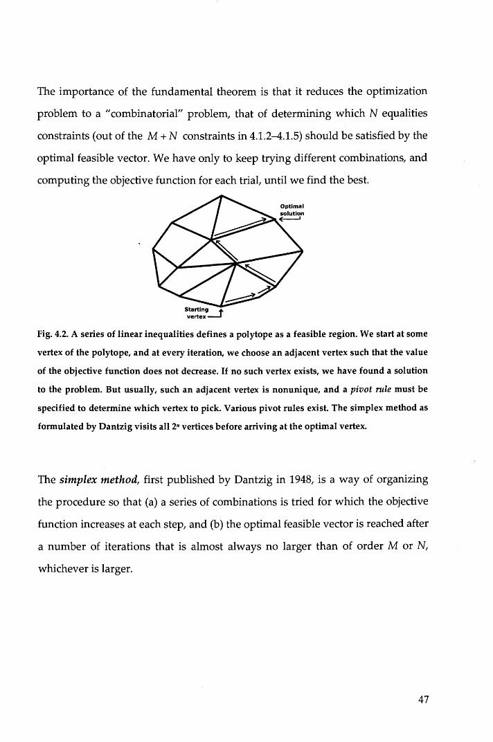
The importance of the fundamental theorem is that it reduces the optimization
problem to a "combinatoria!" problem, that of determining which N equalities
constraints (out of the M+ N constraints in 4.1.2-4.1.5) should be satisfied by the
optimal feasible vector. We have only to keep trying different combinations, and
computing the objective function for each trial, until we find the best.
Fig. 4.2. A series of linear inequalities defines a polytope as a feasible region. W e start at some
vertex of the polytope, and at every iteration, we choose an adjacent vertex such that the value
of the objective function does not decrease. If no such vertex exists, we bave found a solution
to the problem. But usually, such an adjacent vertex is nonunique, and a pivot rule must be
specified to determine which vertex to pick. Various pivot rules exist. The simplex method as
formulated by Dantzig visits ali 2n vertices before arriving at the optimal vertex.
The simplex method, first published by Dantzig in 1948, is a way of organizing
the procedure so that (a) a series of combinations is tried for which the objective
function increases at each step, and (b) the optimal feasible vector is reached after
a number of iterations that is almost always no larger than of order M or N,
whichever is larger.
47
4.3. Simplex Method fora restricted N ormai Form.
A linear programming problem is said to be in normal form if it has no
constraints in the form (4.1.3) or (4.1.4), but rather only equality constraints of the
form (4.1.5) and nonnegativity constraints of the form (4.1.2).
For our purposes, it will be useful to consider an even more restricted set of
cases, with this additional property: each equality constraint of the form ( 4.1.5)
must have at least one variable that has a positive coefficient and that appears
uniquely in that one constraint only. We can then choose one such variable in
each constraint equation, and solve that constraint equation for it. The variables
thus chosen are called left-hand variables or basic variables, and there are
exactly M (= m3) of them. The remaining N -M variables are called right-hand
variables or nonbasic variables. Obviously, this restricted normal form can be
achieved only in the case M ~ N, so that is the case that we will consider.
Any linear programming problem can be transformed into restricted normal
form; there exist a couple of clever tricks that render trivial the task. First, we
need to get rid of the inequalities of the form (4.1.3) or (4.1.4), for example, the
first three constraints in (4.1.7). We do this by adding to the problem so-called
slack variables, which, when their nonnegativity is required, convert the
inequalities to equalities. W e will denote slack variables as Yi . There will be
m1 + m2 • Once they are introduced, we treat them on an equal footing with the
originai variables xi; then, a t the very end, we simply ignore them.
For example, introducing slack variables leaves (4.1.6) unchanged but tums
(4.1.7) into:
48

(4.1.8)
.. (The sign of the coefficient of the slack variable is determined by which sense of
inequality i t is replacing.)
Second, we need to insure that there is a set of M left-hand vectors, so that we
can set up a starting tableau in restricted normal form. (In other words, we need
to find a "feasible basic starting vector"). The trick is again to invent new
variables. There are M of these, and they are called artificial variables; we
denote them by zi. W e put exactly one artificial variable into each constraint
equation on the following model for the example (4.1.8):
(4.1.9)
Our example is now in restricted normal form.
Now one may object that (4.1.9) is not the same problem as (4.1.8) or (4.1.6)
unless all the zi 's are zero. W e must proceed to solve our problem in two
phases. First phase: We replace our objective function (4.1.6) by a so-called
auxiliary objective function
z' =-z -z -z 1 2 3 (4.1.10)
49

We perform the simplex method on the auxiliary objective function (4.1.10) with
the constraints ( 4.1. 9). Obviously1 the auxiliary objective function wili be
maximized for non-negative z; l s if ali the z; l s are zero. W e therefore expect the
simplex method in this first phase to produce a set of left-hand variables drawn ,
from the X;1
S and Y; 1S only1 with ali the Z;
1S being right-hand variables. We then
cross out the Z; l s l leaving a problem involving only X; l s and Y; l s in restricted
normal form. In other words1 the first phase produces an initial feasible basic
vector. Second phase: solve the problem produced by the first phase1 using the
originai objective function1 not the auxiliary.
If the first phase doesn1t produce zero values for ali the z; l s 1 it is the signal that
there is no initial feasible basic vector1 i.e.1 that the constraints given to us are
inconsistent among themselves. Report that fact1 and we are done.
50

4.4. Example of application of the Simplex procedure
As we have just established, the simplex method changes constraints
(inequalities) to equations in linear programming problems, an d then sol ves the
problem by matrix manipulation. The solution set for the altered problems is of
higher dimension than the solution set of the originai problem, but it is easier to
study with matrices.
A Standard maximizing problem (for minimizing the procedure is the same
changed the signs of the coefficients) is a linear programming problem which
satisfied ali of the following four conditions:
1) The objective function is to be maximized.
2) All inequalities are ofthe Stype.
3) All right end constraints are non-negative.
4) All variables are non-negative.
W e show in detail which is the procedure of simplex method applying it in the
resolution of the following LP problem:
MAXIMIZE Z=x1+2x2-x3
SUBJECTTO: 2x1 + x2 + x3 ~ 14
4x1 + 2x2 + 3x3 ~ 28 2x1 + 5x2 + 5x3 ~ 30 x1 ~ O; x2 ~ O; x3 ~ O
Fig. 4.3. Example of linear programming problem.
The Simplex iteration can be summarized in the following 9 steps:
51

1st. Rewrite each constraint (inequality) as an equation.
2nd. Write the revised problem as a tableau, with the objective row (=
bottom row) consisting of negatives of the coefficients of the objective
function Z; Z will be maximized. The lower right corner is the value of
z when xl, x2 ••• are zero; thus, Z usually starts out as zero.
MAXIMIZE z =x,+ 2x2- x3 2x1+ x 2 + x 3 +s1 =14 2 1 1 o o 14 SUBJECT ro:
2x1 + x 2 + x3 ~ 14 m> 4x1 + 2x2 + 3x3 +S2 = 28 g)) 4 2 3 o 1 o 28
4x,+ 2x2 + 3xa ~ 28 2x1+5x2 +5x3 +s3 = 30 2 5 5 o o 30
2X1+ 5X2 +5Xg~30 ALL V ARIABLE S ~ O -1 -2 +l o o o o x,~o;x2 ~o;xa~o
Fig. 4.4. On the Ieft there is the originai problem: objective function is in green. After Stepl,
the constraints are written in equation form introducing auxiliary variables (red variables) that
are called Slack Variables. On the right the SIMPLEX TABLEAU. Compare red symbols with
z = x1 + 2x2 - x3 • Blue numbers are the "ISM"(see text).
The IDENTITY SUB-MATRIX (ISM) is an identity matrix located in the slack
variable columns of the starting tableau, but moving to other columns during
simplex method. A BASIC SOLUTION for a tableau is a vertex of solution set of
the originai system of inequalities. For each tableau, the coordinates of its basic
solution are as follows: all variables not associated with the ISM are set equal to
zero, evaluate other variables by reading each tableau row as an equation.
Simplex method will move the ISM, one column at a time; after each such move,
we arrive at (or "hope" to) a new corner point (basic solution) with bigger
52

objective value. Since the solution set has only finitely many corners, this process
ultimately yields the biggest value of the objective function.
An INDICATOR (for standard maximizing problems) is a number in the bottom
(objective) row of a tableau, excluding the rightmost number. Thus here, the
INDICATOR ROW is the bottom row.
3rd. The PIVOT COLUMN is that column containing the most negative
indicator. If no indicator is negative, the tableau is a FINAL TABLEAU:
see step 8.
4th. Form RATIOS (quotients) for each row: divide the right-most number
by the number in the pivot column of that row.
RATIOS 2 t 1 o o 14 '1 - r3 = R1 2 1 o o 14 14+1
4 2 3 o l o 28 28+2 4 2 3 o 1 o 28 r2 -2r3 = R2
® 2 1 o o 1 6 2 5 o o 1 30 5 5
r4+2r3=R4l -1 -2 +1 o o o o o
TO
~~P!\! OT NEXT LI NE
Fig. 4.5. See steps 3, 4, 5 of SIMPLEX METHOD as we handle INDICATORS, RATIOS, and
PIVOTS. Named above are the 4 row operations (see text) needed to pivot on the number "5"
encircled in red
5th. The PIVOT ROW is the row with the smallest NON-NEGATIVE ratio
(quotient). Note that O +(+l) and O +(-1) are both numerically zero, but
in calculating RATIOS, consider 0+(+1) as positive (OK), and 0+(-1) as
negative (not OK).
53

PIVOTING (or formally, a PIVOT TRANFORMATION) uses row operations to
change one matrix entry (the PIVOT) to "l" (by dividing the pivot' s row by the
pivot number), and then to change all others entries in the pivot' s columns into
ZERO' s (by adding to each row a suitable multiple of the pivot row).
An elementary row operation is one of the following changes made to the rows
of a matrix:
l. Interchanging two rows.
2. Multiplying or dividing each element of a row by the same non-zero
number "c".
3. Adding to a row a non-zero multiple "c" of another row.
6th. Apply a pivot operation to the tableau, including the bottom
(objective) row. The pivot column will become a column of a new ISM
in the new tableau. Note which column is replaced, and where the new
ISM is located; its columns may not be in the usual order.
7th. Note the new basic solution (corner point) far the new tableau.
8th. If all indicators (in the bottom row) are non-negative, stop: the tableau
is a FIN AL T ABLEAU. The basic solution of step 7 is the maximal
solution.
9th. Otherwise, if some indicator remains negative, repeat steps 3 through 9
WITH YOUR NEW TABLEAU. After a finite number of such, simplex
method must terminate at step 8.
54

RATIOS .e o o o 1 a s+i=s) nE: ~
1 11-~r2=R, ®
-5 SEE o o o -5 a
o o 1 -~ 16 16+ :5 BELOW 1 o 5 o 5 1 5 16 1s -a
-'. o o .l 6 (~)r2=R2 -'. 1 o o ! 6 r3- ~r2= R3 5 5 5 1 o 3 o o ~ 12 o 3 o o -'. 12 r4 +!r2=R4 -5 5
~PIVOT TO COLUMN) MATRIX
BELO W
Fig. 4.6. The results of the row operations named above, blue numbers are the new ISM. Since
one INDICATOR (namely -1/5) remains negative, we must repeat steps 3-9. Named above are 4
row operations needed to pivot on the number (16/5) encircled in red.
Above there was a tie for least non-negative ratio: either row1 or row2 could have
become the pivot row, and either choice leads to the final tableau after one
additional pivoting. Below is the result of the final 3 row operations.
Xt x2 xa s, s2 Ss
o o 1 1 o o -2 -2
o 5 o ~ 1 5 16 16 -a o i o 1 1 4 -a 4 o o 49 o 1 3 13 16 16 8
INOICATOR
Fig. 4.7. Ali indicators are now zero or bigger. Thus the last tableau is a Final Tableau. Row
operations of Simplex Method are done.
All indicators are now zero or bigger ("13" is not an indicator). Thus, as in step 8
of the SIMPLEX METHOD, the last tableau is a FINAL TABLEAU. Row
operations of SIMPLEX METHOD are done.
55

Thus, the basic solution for the tableau above is the solution to our originai
problem.
l. set equal to O all variables NOT associated with the blue ISM, as at the
right. Each column of the final tableau has a label naming its variable.
2. convert each row of the final tableau (except the bottom row) back into
equation form (see below) to find the values of the remaining variables.
3. The value of the objective function is in the lower right corner of the final
tableau.
= o Ox1+ Ox2- ix9 + 1s1 - !s2 + Os9 =O or s1 =o
1x1+0x2 +ix9 +os1+i's2-'bs9 =5 or x1=5
O 1 7 1 1 x,+ x2 + eXg+ Os1- 8s2 +4Sg=4 or
ANO Z= 13
Fig. 4.8. The basic solution for the tableau above is the solution to our originai problem.
56

5. Numerica! solution of the inverse problem
5.1. lntroduction
During the last decade severa! attempts were undertaken to solve the inverse
problem for the source of a particular earthquake, that is to determine the spatial
and temporal distribution of sii p or slip rate over the fault area, using teleseismic
as well as locally recorded waves. The solution of ali these problems is far from
trivial. lt is well known that this inverse problem is unstable, even in the
imaginary case of a continuous distribution of seismic stations over the surface of
the Earth and its instability and uniqueness properties have been discussed in
Kostrov and Das (1988). From the computational point of view, this instability is
equivalent to the non uniqueness of the solution. The real situation is even worse
because the number of stations with appropriate records is very limited.
Consequently, to obtain a definite solution of such a problem, one needs some
physical constraints on the source process, in addition to the requirement of
fitting the observed seismograms. In principle, these constraints should be
inferred from the physics of faulting during the earthquakes, that is, from
fracture and frictional mechanics. Unfortunately, our knowledge of the physics
of the earthquake process is stili rather limited and the only comparatively well
established constraint is the limitation on the fracture propagation speed. This is
a weak constraint because the duration of the earthquake process is greater than
the seismic waves propagation time across the fault whereas the limiting
fractures speed is comparable to the seismic wave velocities. To implement these
57

constraints numerically, one requires very fine spatial griding on the fault. A less
physical founded constraint would be the requirement that the slip rate vector be
directed in accordance with the average stress drop direction, that is the
projection of the slip rate vector in stress drop direction must be positive. While
in principle slip in the opposite direction is possible due to interference of waves
on the fault, it does. not seem likely and experience from three dimensionai
forward modeling shows that the slip direction almost coincides with that of
stress drop (Das, 1981 ). This suggest that with sufficient practical accuracy one
may assume the slip direction to be constant over the fault during the process
and coincide with the stress drop direction and the only component of the slip
rate vector to be non negative (no back-slip constraint).
Other physical constraints may be considered. For example one may require the
solution to be in agreement with the seismic moment obtained from the centroid
moment tensor solution or from geodetic measurements.
To invert for the three dimensionai slip rate distribution (two spatial dimensions
on the fault and time) is a computationally difficult task. With sufficiently fine
griding of the fault, it is also impracticable in a regular way, even on existing
supercomputers. Not surprisingly simplified methods of solving the problem
have been used. Basically some simplifications are always a version of trial and
error fitting. In any case the method of the solution imposes some implicit
constraints. Then when one obtains a unique solution, i t is not clear if it is unique
due to the explicit formulateci constraints or as a result of the method used in the
inversion.
The problem for inversion for spatial and temporal distribution of seismic slip
was first formally solved by Olson an Aspel (1982). In that paper the need for
additional constraints apart from observations is most explicitly discussed and
58

the mathematical aspects of the inverse problem are extensively presented. To
quote them:
"In arder for a particular slip distribution to be an acceptable solution to the
inverse problem it must satisfied the following three conditions.
l. The solution must explain the data.
2. The solution must be physically reasonable ( consistent with independent
constraints ).
3. If more than one solution fits the data equally well, additional information
must be supplied to uniquely define which solution is being obtained."
The third condition means that the physical constraints may be insufficient to
specify a unique solution of the problem and they proposed to include some
additional nonphysical assumptions to make the solution unique. In their paper
they used the requirement that the solution has minimum norm.
For physical constraint Olson and Aspel (1982) used a form of the no-back slip
constraints as well as limiting of the rupture propagation speed. Additionally
they required slipping to be confined to grids intersecting the rupture front and
limited the number of times each grid could slip. Effectively their model
included two preassigned fronts, the rupture front and the healing one between
which the whole slip process was confined. This last assumption permitted
drastic reduction of the numbers of unknowns in the model.
Numerica! solution of the forward problem show that with an inhomogeneous
strength and friction on the fault, the rupture front can became very distinct from
a single line and subsequent slip behind the main rupture front is frequently
obtained (Das and Aki, 1977).
The discretization of the problem can itself imply unwanted constraints on the
solution. Namely, with a coarse grid the number of unknowns can be reduced so
much as to make the corresponding numerica! problem stable, that is well
59

conditioned, without additional physical constraints, the extreme cases being
point source fitting, and fitting the source to a rectangular dislocation with a
constant slip and constant slip rate.
5.2. lnversion for seismic slip rate history and distribution
with stabilizing constraints
Using the representation theorem (3.3.18) the displacement record at a station
located at a point x, on the earth surface can be expressed in terms of the slip
distribution over a fault L as:
t l
uk(x1 ,t1 )= Jdt J JKik(x11 x,t1,t}li(x,t)dS 5.2.1 o ~
where i, k = l, 2, 3, uk (x1 , t1) are the components of the displacement vector,
ai(x,t) are the components of the slip and Kik(x11 x,t1 ,t) are the components of
the impulse response of the medium a t {x1 , t1 ), due to a dislocation point source
a t (x, t). The observed seismograms do not represent the displacement vector u
itself but are filtered by the instrument. Convolving both side of (5.2.1) with the
instrument response for a given station and assuming the slip direction to be
constant, we obtain, after some transformations:
t l
sj {t l)= Jat f fwj(~, t1 - t, t )i(~, t)ds 5.2.2 o ~
60

Where j identifies the stations and components of the seismogram S(t1 ), Wj{~,t)
is the impulse response a t (~,t) corresponding to a fixed sii p direction and
convolved with the instrument response, a(~, t) is the sii p rate, the two
dimensionai vector ~ gives the position on the fault relative to some reference
point (for example the, the earthquake hypocenter) and t is the time measured
from the origin time of the earthquake. With a continuous distribution of
stations, equation (5.2.2) would represent an integrai equation of the first kind.
Such equation is known to be unstable. We shall consider the effect of the
following additional constraints:
a(~,t)~o forall (~,t)
a(~, t)= O for t < T(~)
5.2.3a
5.2.3b
w h ere t = T(~) gives the boundary of the area w h ere sii p is permitted a t time t,
00
Jdt J fu(~)ii(~,t)dS = M 0 5.2.3c o ~
where M 0 is the seismic moment and 11 is the modulus of rigidity of the
medium.
The constraint (5.2.3a) is the #no-back slip constraints", the constraint (5.2.3b) is
the #causality constraints" and the constraint (5.2.3c) is the #seismic moment
constraint". Note that T(~) as defined above is not the usual rupture front, but in
what follows we shall referto this boundary as the causality front to distinguish
it from the usual definition.
61

For the numerica! solution the integrals in (5.2.2) must be discretized (we
consider in more detail this process in the next section) and the equation (5.2.2)
takes the form:
Ax~b 5.2.4
Where A is the matrix obtained by integration of Wj, each column of A being a
set of synthetic seismograms for all stations corresponding to different cells and
time instants of the source duration, ordered in the same way as the observed
seismograms and A and b are appropriately weighted.
So, the inverse problem has been reduced to the solution of a linear system under
one or more constraints. In the system (5.2.4) the number of equation m is equal
to the total number of data samples taken from all the records involved and the
number of unknowns n is equal to the number of cells times the number of time
step at the source. We shall take m greater than n to reduce the influence of the
noise contained in the observations b on the solution. Then, the system (5.2.4) is
overdeterminated and we can only obtain a solution which provides a best fit to
the observations.
It is well known that the matrix A is ill conditioned which implies that the system
(5.2.4) admits more than one solution, equally well fitting the observations. The
constraints are introduced just for the purpose of reducing the set of permissible
solutions.
It remains to formulate in exact form what the best fit to observations means.
W e have to minimize the vector of residuals:
r=b-Ax 5.2.5
62
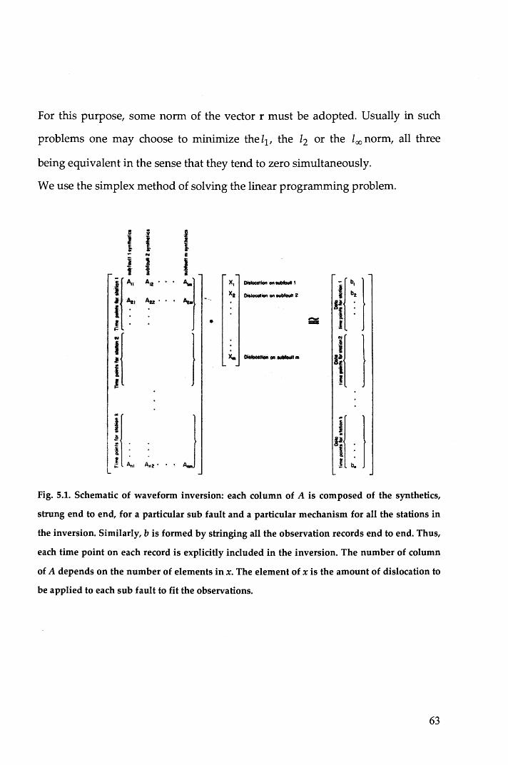
For this purpose, some norm of the vector r must be adopted. Usually in such
problems one may choose to minimize the 11, the 12 or the 100 norm, all three
being equivalent in the sense that they tend to zero simultaneously.
W e use the simplex method of solving the linear programming problem .
i . l .o l i
l N l
j l i l'
~F AIZ • • • :l x, Dillocotlon 01\ ....... t ir 1
X a OitlcH:otiGn Oft IUbfatlll 2 Ati .• Ji . l : ,..., t : l . • - 1 j:
!l l il l x. DilloeotiOII Oft ........,., ftl ~~ t
' .J
"l .. J c
~t! : l l !
l : ! ~~ A11z • l bll
Fig. 5.1. Schematic of waveform inversion: each column of A is composed of the synthetics,
strung end to end, for a particular sub fault and a particular mechanism for ali the stations in
the inversion. Similarly, b is formed by stringing ali the observation records end to end. Thus,
each time point on each record is explicitly included in the inversion. The number of column
of A depends on the number of elements in x. The element of x is the amount of dislocation to
be applied to each sub fault to fit the observations.
63

5.3. The linear programming approach developed by Das
andKostrov
For the numerica! solution1 the integrai equation 5.2.1 which has to be solved has
to be discretized. We divide the rectangular area on the piane into rectangular
cells by equally spaced straight line paraliel to the strike and dip of the fault1 one
celi center coincident with the hypocenter. W e denote the dimensions of the celis
Ax and !!h in the strike and dip direction1 respectively. For each celi the
synthetic seismograms are computed for ali stations with unit slip rate uniform
within the celi and a time step !l r 1 which is taken as the sampling interval of the
slip history. Let the number of celis in the strike direction be N x 1 those in the di p
direction be N h and the number of time steps in the slip history be N t • The
synthetics are sampled with the same sampling interval as the records used for
inversion(llt). We denote the synthetics S(kxlkh 1 j51 jt!!t)1 kxlkh being the celi
numbers along the strike and dip1 and jt the number of the corresponding
seismogram sample at the stationj5
• Let s(kxlkhlkr) be the (unknown) slip rate at
the celi (kxlkh) at the timellrkr. Then the seismograms wili be modeled as:
5.3.1
And the problem consists of finding such s(kxlkhlkr) as to approximate with this
expression the real records a t stationsl say u(j s l j t).
We use a weak causality condition requiring that the first signal recorded at any
station must be radiated from the hypocentral celi. This condition excludes some
64

of the s(kx,kh,kr). We renumber the remaining slip rate values sequentially from
one to n1 , n1 <N x N h N r. Let G(kx, kh, kr) be an integer-value array, containing
zeros for the slip rate values excluded owing too the causality condition and the
sequential numbers of remaining s(kx,kh,kr). We denote so renumbered slip rate
values xi, i= l, ... ,n1 • Similarly we renumber the records samples uUs,jt)
sequentially from one to m1 an d denote them uj, j = 1, ... , m1 • Let the
correspondingly numbered values of S(kx,kh,js,jt~t) be denoted aji' aji
comprising a (m1 x n1 ) matrix A. Then the integrai equation to be solved is
discretized and leads to the approximation problem which we have just seen in
the previous section:
Ax~u 5.3.2
We have just discussed the need of additional constraints. Two constraints are
included here from the very beginning, namely the condition of no back slip:
5.3.3
and the requirement that total seismic moment equals the centroid moment
tensor CMT valueM0 , say:
n t
L:cixi =M0 i=l
5.3.4
Where ci is the medium rigidity at the corresponding celi multiplied by the celi
65

area times 11.-r. A third constraint is already included. Namely we assume that
the slip rate is zero at any cell and time step which would produce a signal
before the first arrivai at any station from the hypocentral cell (weak causality
constrain t).
W e follow the procedure described by Das and Kostrov (1994). W e denote
u- Ax by r. W e will minimize the absolute misfit:
5.3.5
H w e represent r as r + - r- 1 w h ere r/ ~ O 1 rj- ~ O 1 the function f will be linear
And we obtain the following linear programming (LP) problem; minimize:
under constraints:
n l
M 0 - LC;X; =0 i=l
5.3.6
5.3.7
5.3.8
66

The first step of solving such a problem consists on finding a feasible solution, a
set of positive unknowns satisfying the constraint. For our problem it can be
dane analytically. First the moment equation can be solved for one of X;' s, x1
say to give:
Substitution on the first set of equation gives:
Le t
cr. = sgn(u. -a.1 Mo J l l l c
l
an d
{
r:--a. l r. l=
l r.+ l
if aj =l
if aj =-l
if aj =l
ifcrj =-1
Now the equation can be solved for r? to obtain:
5.3.9
5.3.10
5.3.11
5.3.12
67

aj _ ( M 0 ) !n ( Ci ) -a· r. -a. u. -a.1 - - a. a .. -a.1 - x. +r. ' 1 1 1 1 c . 1 ]l 1 c l 1
1 1=2 1
M nt (C) xl =_o -L _i_ xi cl i=2 cl
5.3.13
Ali constraint terms in the right hand side are positive, so making ali unknowns
on the right hand side equal to zero we obtain a feasible solution of the set of
constraints. Moreover, it is a basic feasible solution and the problem is
represented in the restricted normal form. Substituting r? into the expression of
f, we obtain:
5.3.14
Assuming that the real amplitude a t the kth station is (l+ Àk) times the actual
vector v k we split the vector u into the sum
Ns
u=~v. ~ ]s js=l
5.3.15
N s being the number of stations. The unknown adjusted record vector will then
be:
Ns (. )v Ns u*=~1+..1 .. =u+"'v . ..1.
~ ls ls L..J ls ls 5.3.16
js=l js=l
68

We assume that at each station it is possible to decide if the amplitude was
overestimated or underestimated and select the sign of A.js correspondingly.
Denoting the sign by ajs 1Say1 we may replace Ajs by ajs A.js where ali Ajs ~O. Now
replacing u in 5.3.13 an d 5.3.14 by u * 1 we obtain:
5.3.17
an d
At this point it is worth changing notations. First let us expand the vector x to
include ali unknownsl quantities1 i. e. A.i 1 r? 1 rj-ai denoting:
5.3.19
Let B the list of indexes of unknowns xi appearing on the left hand side of eq.
5.3.17 namely:
and N be the list of indexes of unknowns on the right hand sidel namely:
69

W e denote the size of B by m2 and that of N by n2 i. e. set m2 = m1 + 1,
n2 = n1 +N s + m1 -1. N ext w e l et:
t;i = -a•(il(a•(j),N(j) -a•(j),t c;~)} tij = aN(i)VB(j),N(j)(J"B(j)
t .. =8 N .. l] n1+ 8 +],1
Where 8 is the Kronecker' delta:
an d
j = 1, ... ,m1
j = 1, ... , m1 ; i = 1, ... , n1 -1
j = 1, ... , m1 ; i = 1, ... , n1 +N 5 -1
j = 1, ... , m1 ; i = n1 +N 5 , ••• , n2
i= 1, ... , n1 -1
i = 1, ... , n1 + N 5 - 1
i = n1 + N 5 , ••• , n2
Then eqs. 5.3.17 and 5.3.18 take the form:
nz
xB(j) = tjo + LtjixN(i) i=1
nz
f = fo + LfixN(i) i=1
j = 1, ... ,m2
5.3.20
5.3.20
5.3.21
5.3.22
5.3.23
70

This system of equations has the form of the tableau of the simplex method in
restricted normal form and can be represented graphically as shown in Fig. 5.2.
Tableau l
N(i) .:t"N(i) rN(t) #"N( i) B(j) i=l, .... ,n1-J n1 + l, .... ,n1+ N~-1 nt +N., ... ,nt ZB(J)
M r'B(:I) l s F tjo I
tji t,, tjt
T s ZD(rn)
....................... .. 100 -"" .... "" .. ..... '"' ...... - - ---········ SLIP MOMENT
RATES ZB(m,) tm20 tm2t = Ci}C1 Cm~i =O O tm2a =O ROW
SUM CRITERIO N OF l /o Il ROW
MtsFrrs
Fig. 5.2. Graphical representation of the simplex method in restricted normal form for the
system of eq. 5.3.23
Our starting solution is:
XB{j) = tjO
XN(i) = 0
j =l, ... , m 2
i= 1, ... , n2
It is feasible, because t jO ~ O an d correspond to the misfit value of f equal to fo .
These xi with i E B are the basic variables, whereas those with i E N are the
non basic ones. Now the simplex algorithm can be applied to the tableau to
minimize f. In our case, the minimum exist as f is the sum of non negative
values r + an d r- cannot be minimized belo w zero.
71

~
u~ llt*13l ----...w
\ a. v
T1111C81ep l Thne~tepl Tlmutep3
~ l l
r~~~<<r X n
~ }~" .t.zl X.Zl
Xzs =
~~~~<<< x,,
t }-· X12
X.. .t
~<~~s>? ~ }-· A x = u
b.
Fig. 5.3 Simple example of an inverse problem for rupture history. a) Schematic map of fault
used in the inversion. It has three numbered celis along strike, with the hypocentre in celi 2,
shown by the star. The fault is one celi in width down-dip, and three times steps will be used
in the moment rate function. The azimuths to three stations (U, V, and W) are shown by
arrows. B) Visual representation of equation ... for this inversion problem, with the part of the
equation corresponding to celi 1,2 and 3 colour red, green and blue, respectively. The right
band side vector, u, contains the concatenation of the seismograms used in the inversion. The
unknown vector x has seven elements, which for this figure only are labelied with two
subscripts, the first representing the time step, and the second the celi number. There are no
unknown xu and Xt3, since they are excluded by the causality constraint. Each column of the
matrix A contains the concatenated Green Function for one of the unknowns. Note that the
time shifts (exaggerated in the figure) corresponding to the different time steps and to the
differing travel times to the stations from the three celis. Since the celis are ali at the same
depth, there is minimal variation in Green function shape between celis.
72

5.4. Computational considerations
The accumulation of rounding errors during optimization using the simplex
method may lead to a completely wrong solution. Let m denote the number of
rows and n the number of columns of the matrix T, (5.3.17) i.e. the number of
basic and non basic variables respectively. When m and n were of the order of
103, the number of optimization steps is up to several tens of thousand.
A step of the simplex algorithm consists of selection of the most negative
component of f (5.3.18) which determines the pivot column of the matrix. Then
within this column, the element is selected which permits maximum increase of
the pivot unknown. Let ip be the column number. Then the pivot column
number is determined by
( t ·0 J • • J
]p= m~n --;tjip <O J t ..
)lp
5.4.1
Next the unknowns xNUP) and x8(;p)are swapped and the system is solved for the
newx8 •
Let us consider first the pivoting of rows. If, owing to round errors, some t jip
became negative while actually being zero it will be selected as the pivot element
with catastrophic consequences. It should be recalled that in ali our cases the
objective function is non negative by definition and cannot be reduced below
zero. It follows then that if any t1.; =O the corresponding /; must be zero, for
p p
otherwise the objective function would be unlimited from below. It means then
that the pivot column was selected mistakenly, /; being negative owing to p
73

rounding errors. To protect from this situation we select some 8 >O of the order
of uncertainties in the elements of the matrix A (of the synthetic seismograms).
The row selection rule is replaced by:
( t.0 ) • - • J •
]p- m~n --~tjip < -8 J t ..
Jlp
5.4.2
If ali t jip ~ -8 the column pivoting is discarded an d the i P th column is marked
not to be selected at subsequent step. When the starting tableau is constructed
the coefficient fi are obtained by summation of misfit rows. We select the
maximum by absolute value of !i l f max l sayl and consider if max as the
uncertainty measure for /; values in ali subsequent step of the algorithm. Then
the column selection rule is replaced by
5.4.3
lf ali fi > -q max we consider the solution to be the optimal one. Strictly speaking
this is not yet optimum for some other problem under consideration but it is the
optimum for some other problem with the matrix A* different from A within the
uncertainty 8 . The role of 8 in the row pivoting and that in the column pivoting
is different. When pivoting a row1 a sufficiently large 8 protects from division
smali numbers and1 consequently from inverting a badly conditioned matrix, but
with column pivoting the large 8 lead only to a premature stopping of
optimization. The two 8 values are chosen different to obtain a solution closer to
the exact optimal one. W e denote this latter 8 by 8 1 •
74

Finally some components of t0 may be made negative owing to rounding errors.
If unprotected, these components grow to large negative value and the object
function increases instead of decreasing. To protect from this, the t0 is inspected
at the end of each step and ali negative components are zeroed out.
These modifications do not eliminate the problem of accumulating of rounds
errors. Because of the large number of steps and the fact that, in the simplex
algorithm pivoting does not select the best element of the tableau matrix with
respect to rounding error, the problem becomes distorted in the course of
optimization. To reduce this error accumulation, we refresh the tableau after
every few thousand steps of the simplex algorithm. The refresh is done as
follows. Let B0 an d N 0 the list of basic and n9n basic variables respectively, a t
the beginning of the optimization, whereas B and N are this list when
refreshing. W e construct the list ENTER containing the variables indexes present
in B and not present in B0 and the list LEA VE for those present in B0 but not
in B . First we construct the originai tableau as a t the beginning of optimization.
Then we use the same algorithm of swapping variables from ENTER and LEA VE
as in the simplex method but with different pivoting. Namely for each variables
to leave the basis jP th, say, we select the index from ENTER, iP such that
5.4.4
This is equivalent to matrix inversion with partial-row pivoting. The number of
swapping steps is equal to the size of ENTER list and is much less than the
number of steps involved in the optimization. Both better pivoting and reducing
the numbers of loops give rise to a !esser error accumulation. To check the
75

accuracy of the solution we calculated the sum of the absolute values of misfit by
direct substitution of x into r = u - Ax and compared this value with the final
value of the object function obtained by the misfit optimization.
76

6. Outline of the geology of Iceland
6.1. Geologica! and Geotectonic Setting
Iceland is located at the junction of the two large subrnarine ridges, the Mid
Atlantic Ridge and the Greenland-Iceland-Faeroes Ridge, which are parts of the
global rnid-oceanic ridge systern. Mid-oceanic ridges rnark divergent boundaries
between tectonic plates (Fig la). Iceland is regarded as being a hot spot above a
rnantle plurne, and has been piled up through ernissions of volcanic rnaterial and
grown by rifting and crust accretion through volcanisrn along the axial rift zone
(Fig lb). The rift zone, in terrns of the plate tectonic frarnework, rnarks the
boundary between the Eurasian an d N orth Arnerican plates.
ICELAND
Fig. 6.1. a) Map showing the Mid-Atlantic Ridge splitting lceland and separating the North
American and Eurasian Plates. The map also shows Reykjavik, the capitai of lceland, the
Thingvellir area, and the locations of some of Iceland's active volcanoes (red triangles),
in d u ding Krafla (http:/ /pubs. usgs.gov /pub Ii ca tions/text/understanding.html #anchor556 7033).
b) Cross-Section of lceland. There is a debate in the scientific community whether the hot
materia! or magma beneath Iceland originates from the upper mantle or rises as a hot, buoyant
piume from the lower mantle or core-mantle (http://www.lonker.net/nature_geology_3.htm)
77

Accordingly the western part of Iceland, west of the volcanic zones, belongs to
the North American plate and the eastem part to the Eurasian plate. Iceland is
one of the few places on Earth where an active spreading ridge can be observed
above sea level. As new crust is created along the rift zone, old bedrock moves
further from the plate boundary. Therefore, the oldest rocks exposed on the
surface in Iceland, formed about 16 million years ago, occur in the eastemmost
and westemmost parts of the country. Oldest rocks in the Iceland basalt plateau,
nowhere exposed on the surface, may be 25 million years old. The mechanism
which causes tectonic plates to move is probably related to slow-moving
convection currents within the mantle and to pull created when plates sink back
into the mantle at convergent plate boundaries. It is the combination of a
divergent p late boundary and hot spot that has led to the formation of Iceland.
6.2. Bedrock forrnations
The geologica! record in Iceland spans about 16 million years. Iceland is built
almost exclusively of volcanic rocks, predominantly basalts (Fig. 2a). Silicic and
intermediate rocks - rhyolites, dacites and andesites - constitute about 10% and
sediments another 10%. The rocks of Iceland can be divided into four main
formations (Fig. 2b): (l) The Tertiary Basalt Formation (TBF), (2) The Upper
Pliocene and Lower Pleistocene Grey Basalt Formation (PPF), (3) The Upper
Pleistocene Palagonite (Hyaloclastite) M6berg Formation (UPF) and (4) The
Postglacial formation (PGF), which besides postglacial lavas includes sediments
as till and glacial sediments from the retreat of the last ice cover and marine,
fluvial and lacustrine sediments and soils of Lateglacial and Holocene age.
78

Fig. 6.2. a) Geologica! map of Iceland, showing volcanic systems and bedrock formations. b)
The lcelandic bedrock formations: l) Tertiary Basalt Formation; 2) Gray Basaltic Formation,
late Pliocene and early Pleistocene; 3) Moberg Formation, late Pleistocene. (Source:
http://www.hi.is/%7Eoi/index.htm)
The Tertiary Basalt Formation (TBF) mainly appears in two large regions on
eastern and western-northwestern Iceland, on either side of the active rift zones
transecting the country (Fig. 2b ). Altogether TBF constitutes about half the
country's area. The stratigraphic thickness of TBF is -10 km. Volcanics make up
>85% of the TBF. Basaltic lava flows, mainly tholeiitic, form most of the volcanic
pile above sea-level. Silicic (rhyolitic) and intermediate rocks and detrital beds
form the rest. Dykes are common and intrusions of gabbro and fine-grained
granite (granophyre) occur, especially within remains of ancient centrai . volcanoes. The TBF is regarded as spanning the period 16-3.3 million years. The
oldest rocks which have been dated with radiometric methods are about 14
million years old, or of Middle Miocene age. The TBF becomes successively
younger towards the rift zones, reflecting drift tectonics.
The Upper Pliocene and Lower Pleistocene Grey Basalt Formation (PPF) is
confined mainly to a broad SW-NE trending zone between the Tertiary plateau
79

basalt areas and the active rift zone (Fig. 2b ), and on the peninsulas of Tjomes
and Skagi in northem Iceland and Sn~fellsnes in western Iceland. The PPF spans
the time period 3.3-0.7 million years, and the cumulative thickness of the
formation is about 2 km. The bedrock in the Reykjavik area mostly belongs to
PPF.
The Upper Pleistocene Palagonite (Hyaloclastite) M6berg Formation (UPF)
consists of rocks that are younger 0.7 million years. The distribution of UPF rocks
is mostly within the active volcanic- and rift zone (Fig. 2a).
6.3. Earthquakes
The earthquakes in Iceland may be divided into three main categories, reflecting
the main triggering mechanisms:
• Tectonic earthquakes are due to relative movements of the North
American and Eurasian Plates. These are the biggest earthquakes and may
reach magnitude seven or even more.
• Volcanic earthquakes are attributable to volcanic activities as the main
source of triggering. These earthquakes are generally located in the
vicinity of well-known volcanoes, and their magnitude will hardly ever
exceed magnitude six. This type of earthquake does not normally have
any significant effect on engineered structures.
• Geothermal earthquakes, usually not exceeding magnitude three, are
small tremors occurring quite frequently in high-temperature geothermal
areas. They do not have any significant effect on engineered structures.
80

In addition to these naturally triggered earthquakes, the so-called man-made
quakes should be mentioned to complete the picture. They are assigned
primarily to the activities of man, e. g., the filling of reservoirs and rock blasting.
The tectonic earthquakes in Iceland are of two types, i.e., interplate earthquakes,
related directly to plate boundaries, and intraplate earthquakes originating
inside the plates. The interplate earthquakes in Iceland can be divided into two
groups, depending on the piace of origin. In the first group, earthquakes
originate in the spreading zone between the plates, i.e., on the Mid-Atlantic
Ridge. These earthquakes are rather small, with magnitudes that seldom exceed
five. The source mechanism can be complex. In the second group, earthquakes
originate in the fracture zones, which we consider more in detail in the next
section. They are the biggest earthquakes in Iceland, and their source
mechanism, obtained by fault piane solutions, is, in all cases, of a strike slip type.
The seismic motion projected for the South Iceland Seismic Zone on the basis of
plate tectonics, which is left-lateral on the east-west striking fault, is,
nevertheless, not visible on the surface as a major surface fracture. It appears, on
the contrary, that the motion can be visualized as a series of north-south striking,
right-lateral faults. This is supported by the geologica! evidence of fault traces on
the surface as well as by the north-south, elongated shape of the mapped
destruction zones of large, historical earthquakes. In the northem seismic area,
this is not as obvious since the epicentral areas are mostly beyond the coast.
The intraplate earthquakes in Iceland are not as frequent as the interplate
earthquakes.
81

6.4. The South Iceland Seismic Zone
Iceland is a superstructural part of the Mid-Atlantic Ridge, which continues in
the SW on land as the Reykjanes Peninsula (RP) oblique rift zone. Aèross Iceland
from southwest to the north, the rift zone is displaced towards the east through
two major fracture zones or transform faults. These are the South Iceland Seismic
Zone (SISZ) and the Tjomes Fracture Zone (TFZ), indicated on Fig. 6.3.
Fig. 6.3. Main tectonic structures and earthquake epicenters. The grey areas indicate volcanic
zones; solid lines indicate rift zones offshore representing parts of the Mid-Atlantic Ridge; the
rift zones on land are located at the Eastern, the Western and the North Volcanic zones; dashed
lines indicates fracture zones offshore and seismic lineation; SISZ is the South Iceland
Seismic Zone; TFZ is the Tjornes fracture Zone; WIFZ is the W est Iceland fracture Zone; white
cirdes denote earthquake epicenters (Ambraseys and Sigbjornsson, 2000); red cirdes show
epicenters of events recorded by the Icelandic Strong-motion Network during the South
Iceland earthquake sequence in June 2000; the average motion of the Eurasian Plate and Nòrth
American Plate is indicated by the bold arrows. (From Sigbjornsson and Olafsson, 2004)
According to the NUVEL lA plate model (DeMets et al. 1994) the direction of the
divergent motion across the plate boundary of the Eurasian relative to the N-
82

American plate in Iceland is N103°E at a velocity of 1.85 cm/year. If ali of this
motion is taken up by the SISZ, which is oriented almost towards EW, the
relative left-lateral motion across SISZ would be approximately 1.8 cm/year and
a NS opening component across the zone could be around 0.4 cm/year.
Fig. 6.4. The south-western part of Iceland. Iceland as a whole is shown in the upper right
corner. Dotted yellow lines denote the western volcanic zone (WVZ) and the eastern volcanic
zone (EVZ). The South Iceland seismic zone (SISZ) is indicated as well as its prolongation in
the Reykjanes peninsula (RP). The direction of the relative plate motion is shown by arrows.
The faults of the two large earthquakes that ruptured on June 17 and 21 are indicated by 17
and 21 respectively. The epicenters of small shocks following the large earthquakes (red dots)
show the extent of the seismically activated area.
(from http:/ /bra un. ve d ur .is/j a/prepared/SouthlcelandEarthq2000)
Many large (Ms > 6) earthquakes have occurred in the SISZ since Iceland was
settled in the ninth century A.D. Historical accounts describe sequences of large
earthquakes over a period of days to years, starting with an earthquake in the
eastern part of the SISZ and continuing with events of equal or smaller
magnitude further west.
83

Most of the earthquakes in this EW left-lateral shear zone have had right-lateral
motion on NS striking faults as observed on the surface. Faults due to known
historical earthquakes are found side by side a t less than 5 km distance from each
other (Einarsson, 1991; Einarsson et al., 1981; Stefansson et al., 1993). There are
indications, based on historical seismicity and tectonic considerations (Stefansson
and Halld6rsson, 1988), that the seismic cycle, i.e. the time period of strain build
up and of break-up (strain release) of the whole SISZ is about 140 years.
Severallarge historical earthquakes in the SISZ have, however, occurred as single
events. The 1912 event (Ms = 7 .0) was the first SISZ earthquake to be
instrumentally recorded (Bjamason et al., 1993). Following the 1912 earthquake,
the SISZ was seismically relatively quiet until June 2000.
6.5. Short term precursors of the June 17 earthquake
While the June 17 earthquake occurred in the area identified as the probable
location of the next large earthquake in the SISZ, no short-term precursory
signals were recognized before it occurred. In hindsight, however, several
changes can be recognized, changes that were possibly premonitory. These
include (from Stefansson et al., 2003):
1) Several microearthquakes (ML=0-1) clustered a t depth along the fault of the
impending earthquake, weeks and days before its occurrence (Figure 6.5). This
was a significant change compared to the less clustered microearthquake activity
that had been observed during the previous 10 years.
2) In a geothermal borehole at Fluoir 10 km to the north of the NS striking fault
piane (Figure 6.5), short-term water level drop, of not less than 5 m, was alarmed
24 hours before the earthquake. Unfortunately this signal is not seen in the
84

preserved recorded trace averaging water level on 15 minutes intervals. During a
5 years of continuous operation this was the first such an alarm (Bjomsson et al.,
2001). Most probably the alarm was a short-lived low pressure pulse related to
the preparatory phase of the earthquake. Both these changes were possibly
related to relocation of strains towards the impending rupture, possibly related
to dislocation in the deeper and ductile part of the seismic zone.
Severa! other observed changes, listed below, prior to the earthquake may
possibly also be related to a crustal process leading to it:
l) The volcano Hekla (Figure 6.4), 30-35 km east of the epicenter, has been
anomalously active since 1970, last erupting at the end of February 2000. An
eruption with similar mechanism occurred in 1991. In that case a flurry of small
earthquakes followed in the SISZ during days and weeks (Stefansson et al., 1993).
There are also earlier examples of this effect which probably is caused by transfer
of strain energy along a seismically active zone where local spots are dose to
fracture criticality, even if the area is not ready for a large earthquake. Thus it
was considered noticeable that small earthquakes did not occur in the zone
following the February 2000 eruption. After the large earthquakes occurred in
the zone it is tempting to suggest that this lack of earthquakes is comparable to
periods of quiescence sometimes reported before large earthquakes. It remains to
be studied what is the mechanism of stress transfer in the region and how this
may explain the flurry of small earthquakes frequently observed as well as the
lack of it this time. Better understanding of this may lead to the application of
such a quiescence as a precursor.
2) A slight but persisting increase in seismicity was observed in the SISZ area
early in 1995-1996 (Guòmundsson et al., 2001). On a long-term scale the seismic
rate in the SISZ was slightly increasing since that time. This may have been
linked to dyke intrusions in Vatnajokull area, 150 km towards northeast in the
85

eastern volcanic zone, preceding the large Vatnajokull eruption in October 1996.
Such a mechanism was proposed (Volti and Crampin, 2003) to explain increased
stress in the area indicated by shear-wave splitting.
Fig. 6.5. The area near the June 17 earthquake. The epicenter is shown by a green star and the
rupture is indicated with a red NS striking line. The NS striking black lines indicate old
earthquake faults. Red dots show microearthquakes (36 in number, ML=-1 to 1), during a
period of 17 days before the earthquake. Hydrological changes were observed at the village
FluèHr. (from http:/ /hraun.ved ur .is/j a/prepared/SouthlcelandEarthq2000)
There were also marked and possibly related changes in seismic rates at different
parts of the zone, especially during the last 1-2 years before the earthquake.
Automatic fault piane solutions of microearthquakes showed anomalous
variations during 3 months before the earthquakes, 20 km to the west of these,
and inside the SISZ (Stefansson et al., 2000).
3) Radon anomalies, i.e. anomalously low values and positive spikes were
observed in radon from geothermal water wells in the area during 1-5 months
before the earthquakes (Einarsson et al., 2003).
86

4) Anomalous strain signals were observed in May and June at borehole
strainmeter stations, 3 and 20 km respectively from the epicenter of the June 17
earthquake.
5) There was some increase in shear-wave splitting time in microearthquakes of
local origin, a few weeks before the earthquake (Stuart Crampin, 2000, personal
communication; Volti and Crampin, 2003).
6.6. The Icelandic Strong Moti o n N etwork.
The Icelandic Strong-motion Network, established in 1984, is based on a small
scale network proposed and installed in the early seventies. An extensive
description of the ISMN is reported in Sigbjornsson and Olafsson (2004). The
objective of the network, according to their promoters, is to collect earthquake
engineering data required for rational structural design and risk management.
The locations of the stations in the network were selected on the basis of the
geophysical information, the geographic distribution of the population, locations
of industriai and power plants as well as the main life-line systems. In most cases
the ground response stations are located inside buildings. There are two main
reasons for this. Firstly, Iceland' s severe clima tic conditions make i t difficult and
expensive to operate sensitive equipment outdoors. Secondly, in order to comply
with the above-mentioned objectives, they judged important in interpreting and
modeling earthquake action on structures and earthquake-induced structural
response, that the obtained data represent the direct seismic effects on the
structural foundations. In most cases, the building foundations are relatively stiff
and have dimensions much smaller than the dominating earthquake
wavelengths for the frequency range of main interest. It is therefore assumed that
87

the recorded data represents free-fieid motion fairly well in most cases
(Ambraseys et al., 2002). The geographicai distribution of the ground response
stations and the arrays in structures are shown in Fig. 6.6, using appropriate
signatures to indicate the type of station.
Norih Atlanti c Ocean
Fig. 6.6. The lcelandic Strong-motion Network. The following notation is used: • ground
response station; bridge; • building; .._ power plant; .A. earth fili dam. Height above sea
leve! is indicated using the following colour code: green 0-200 m; yellow 200-600 m; brown
> 600 m. The white areas are glaciers. Note that the distance between the meridians at 63°
parallel is- 50.5 km. (from Sigbjornsson and Olafsson, 2004)
Further details of the network are given in Tabie 6.1. The Iceiandic Strong Motion
Network consists of 34 ground response stations and arrays measuring ground
motion and structurai response. The network runs with a high degree of
automation, using digitai instruments, with the exception of three analogue
instruments recording on a film. The individuai stations and arrays are
connected to a centrai computer that records detected events, when the
acceieration exceeds a prescribed threshoid. Afterwards the re~ordings go
through a routine processing andare then finally transferred to a database.
88

No
100
101
102
103 104
105
106
107 108
109
110 111
112
113
201
202
203
204 205
301
302 303
304
306 303
307
308
310 311
401
402 403
501 502
Sltename Long La t
ln.strument type Structures a w ON
Aeykjavlk 21.96 64.14 Kinemetrics SMA-1 Unlverslty buildlng, 3 story Salfoss 21.00 63.94 Terra DCA-333 Hospltal, 3 story
Hveragerdl 21.19 64.00 Geotech A-700 Ctmrch Kaldarholl'l 20.47 64.00 Terra DCA-333 Farm house, 2 story Thorlakshotn 21.38 63.85 Klnemetncs SMA-1 SChool b!Jlldlng, 1 story Hefla'l 20.39 63.84 Klnemetncs ETNA SChoot bulldlng, 2 story
Flagb)arnarholt 20.26 63.99 Kinemetrlcs SSA·1 Farm house, 2 story Thjorsartun 20.65 63.93 Geotech A-700 Farm house, 2 story Mlnni-Nupur 20.16 64.05 Kinemetrlcs ETNA Farm house, 2 story Solhelmar t) 20.64 64.07 Klnemetrlcs ETNA Schoot b!Jlldlng, 2 story Hvltarbakkl 20.39 64.16 Terra DCA-333 Farm house, 1 story Selsund 'l 19.95 63.94 Kinemetrics SMA-1 Farm house, 1 story Selfoss, Radhus 21.00 63.94 KMI K2 (array) "' Office bulldlng, 3 story
Hveragerdl, Grund 21.19 64.00 Kinemetrlcs K2 Aetlrement home, 2 s1ory
Dalvlk 18.53 65.97 Kinemetrlcs SSA-1 Offlce bulldlng, 3 story Husavik 17.36 00.05 Klnemetncs K2 Fire Statlon, 3 story Saudarkrokur 19.64 65.74 Klnemetrlcs SSA-1 Schoof bulldtng, 2 story Slgluf):>rOur 18.91 66.16 Klnemetrlcs SSA·1 Retlrement home, 3 slory Kopasker 16.44 66.30 Klnemetrlcs SSA-1 House, 1 story
Burfellsvirkjun 19.84 64.10 HPIKMI (array} a1 Hydroelectrlc power statlon
Hrauneyjarfoas 19.24 64~20 KMI K2 (array) ~ Hydroelectrlc power statlon SUltartangastifla 19.57 64.19 HPIKMI (array} il) Earlh-fill dam Slgoldustlfla 19.10 64.16 HP/KMI (array} Al Earlh-flll dam lrafossvlrkjun 21.01 64.09 KMI SSA·1 (array) 4) Hydroelectrlc power station Ljo&afossvlrkjun 21.01 64.10 KMI K2 (array) 5oi Hydroelectrlc power statlon SJgolduvlrkjun 19.13 64.17 Klnemetrics K2 Hydroelectrlc power statlon SUitartangavlrkjun 19.60 64.15 KMI K2 (array) 6'1 Hydroelectric power statlon
Laxarvlrkjun 17.31 65.82 Kinemetrlcs SSA·1 Hydroelectrlc power statlon Blondustltla 19.67 65.23 KMI SSA-1 (array) "> Earlh-flll dam
Rvk., Hus Versi. 21.90 64.13 KMI SSA-1 (array} 41 Ofllce bulldlflg, 14 s1ory ~
Rvk., Foldaskoli 21.79 64.13 Klnemetrlcs SSA.-1 School bulldlng, 2 story Rvk., Heldmork 21.76 64.07 Klnemetrlcs SSA-1 WeH-house/pump statlon
Oseyrarbru 21.21 63.88 KMI SSA-1 (array} 4l Concrete bridge 9l Thjorsamru 20.65 63.93 KMI K2 (array) 5! Stesi arch bridge ~ 'l Slte-dependent magnlflcatlon observed ~ Concrete shear walls
-4t lnciudlng one ground response statlon 5l lncludlng two groond response stations 'l lnciudlng three ground response stations ~ Bridge YAth selsmlc base lsolatlon
Type
FF FF
FF
FF FF
FF
FF
FF FF
SA
FF SR
SR
FF
SA
SR
FF
FF FF
SR
FF FF
SR
SR FF
FF
SR
SR DR
SR
FF FF
SR SR
Table 6.1. An overview of the Icelandic Strong-Motion Network. Listed are ground response
stations and arrays in buildings and structures. Each ground response station contains one tri
axial sensor. The sensors are located in buildings or structures on firm ground. Sensors from
Kinemetrics are applied in arrays. The trigger thresholds are in the range 0.002 to 0.009 g, but
are in most cases around 0.004 g. Type of the Station is described as: FF - free field, SR -
structure related free field, DR- dam related free field. (From Sigbjomsson et al., 2004)
The data recorded by the Icelandic Strong-motion Network is now freely
available through the ISESD. Website, http://www.ISESD.hi.is. The information
provided is: raw data, i.e. uncorrected time series, corrected acceleration series,
89
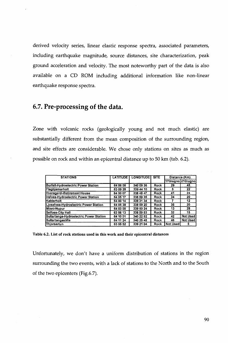
derived velocity series, linear elastic response spectra, associated parameters,
including earthquake magnitude, source distances, site characterization, peak
ground acceleration and velocity. The most noteworthy part of the data is also
available on a CD ROM including additional information like non-linear
earthquake response spectra.
6.7. Pre-processing of the data.
Zone with volcanic rocks (geologically young and not much elastic) are
substantially different from the mean composition of the surrounding region,
and site effects are considerable. We chose only stations on sites as much as
possible on rock and within an epicentral distance up to 50 km (tab. 6.2).
STATIONS LATITUDE LONGITUDE SI TE Distance (Km} 17Giugno 21Giugno
Burfeii-Hydroelectric Power Station 64 06 00 340 09 36 Rock 29 45 Flagbjarnarholt 63 59 28 339 4410 Rock 5 22 Hveragerdi-Retirement House 64 00 07 338 48 47 Rock 41 24 lrafoss-Hydroelectric Power Station 64 0517 338 59 35 Rock 34 20 Kaldarholt 64 0014 339 31 34 Rock 7 12 Ljosafoss-Hydroelectric Power Station 64 05 38 338 59 20 Rock 35 20 Minni-Nupur 64 03 00 339 50 24 Rock 13 28 Selfoss-City Hall 63 56 13 338 59 53 Rock 32 15 Su ltartanga-Hyd roelectric Power Stati o n 6410 01 340 22 52 Rock 42 Not Used Sultartangastifla 6411 24 340 25 48 Rock 46 Not Used Thjorsartun 63 55 52 339 21 04 Rock NotUsed 5
Table 6.2. List of rock stations used in this work and their epicentral distances
Unfortunately, w e don' t ha ve a uniform distribution of stations in the region
surrounding the two events, with a lack of stations to the N orth an d to the South
of the two epicenters (Fig.6.7).
90
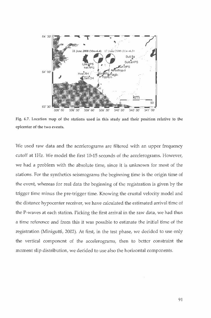
64" 30' FF-~=--==-IIIIF=-P::=--==--:::.=--==-/,.,.-::=--==--=~
i, " '·/
64" 00'
50
338" 00' 338" 30' 339" 00' 339" 30' 340" 00' 340" 30' 341 " 00'
Fig. 6.7. Location map of the stations used in this study and their position relative to the
epicenter of the two events.
We used raw data and the acceierograms are filtered with an upper frequency
cutoff at 1Hz. We modei the first 10-15 seconds of the acceierograms. However,
we had a probiem with the absoiute time, since it is unknown for most of the
stations. For the synthetics seismograms the beginning time is the origin time of
the event, whereas for reai data the beginning of the registration is given by the
trigger time minus the pre-trigger time. Knowing the crustai veiocity modei and
the distance hypocenter receiver, we have calcuiated the estimated arrivai time of
the P-waves at each station. Picking the first arrivai in the raw data, we had thus
a time reference and from this it was possibie to estimate the initiai time of the
registration (Minigutti, 2002). At first, in the test phase, we decided to use oniy
the verticai component of the acceierograms, then to better constraint the
moment slip distribution, we decided to use aiso the horizontai components.
91

6.8. Crustal structu:~;e beneath Iceland
Some basic knowledge on the geology of the South Iceland plain is needed for
the interpretation of the strong-motion data. The surface geology is mostly
formed during and after the last ice age as a pile of basaltic lavas, as well as tuff
layers, often with intermediate layers of sediments or alluvium. The youngest
lavas are from the Holocene (not more than couple of hundred years old),
whereas the oldest formations are up to 3.3 million years old. In the glacial
period Iceland was covered with a plateau glacier. During warmer interglacial
periods the ice melted and the glaciers retreated, which resulted in sea level
changes up to a couple of hundred meters. The South Iceland plain was then
partly a seabed, accumulating marine sediments. During warm periods, and
towards the end of the Pleistocene, when the glacier was retreating and the land
rising, glacial streams formed thick sediment layers, composed chiefly of sand
and fine-grain gravel. In the postglacial period, some of these sediments were
covered by lava, which adds to the complexity of the geologica! structure near
the surface. The lava layers may be as thick as 10 m while the sediment layers
can be up to 20 m thick or even more (Einarsson, 1994). The shear-wave velocity
in basaltic rock is typically in the range 2 to 2.8 km/s, depending on how dense
the rock is, while the shear-wave velocity in tuff and sedimentary rock is,
respectively, 850 m/s and 1000 m/s on the average. The complexity of the surface
geology characterized by the lava piles, tuff and sedimentary formations, is
augmented further by fractures, fissures and faults of tectonic origin
(Sigbjornsson and Olafsson, 2004).
92

6.9. The structural model
Early explosion seismology studies of the crust beneath the Iceland transverse
ridge used P-phase arrivai times. These, along with an early surface wave study,
were interpreted in terms of simple layered models (Bath, 1960; Tryggvason,
1962; Palmason, 1971; Zverev et al., 1976; Bott & Gunnarsson, 1980). In a
pioneering experiment in 1959, Bath (1960) recorded data on two unreversed
explosion profiles z150 and z250 km long in western and centrai Iceland. He
interpreted the times of first arrivals in terms of a three-layered model and
observed reflections he concluded to come from the Moho at a depth of z28 km.
Tryggvason (1962) constructed standard surface wave group-velocity dispersion
curves for Love and Rayleigh waves from 20 earthquakes along the mid- Atlantic
ridge up to z1000 km from Iceland, and also interpreted the results in terms of a
three-layered structure. Palmason (1971) gathered data on z40 profiles up to :::::150
km long covering most of Iceland, and processed the data using conventional
seismic refraction theory. He emphasized the latera! heterogeneity of the
Icelandic crust, and developed layered models involving average velocities and
interface depth ranges. In 1972 Zverev et al. (1976) and Bott & Gunnarsson (1980)
shot the z450 km long profile, which extended almost the entire length of the
Iceland-Faeroe ridge and was recorded at stations on the Faeroe Islands, Iceland,
and the ridge itself.
As soon as waveform modelling was applied to explosion seismology data from
Iceland it became clear that Icelandic-type crust is most naturally subdivided on
the basis of velocity gradient. Flovenz (1980) reinterpreted explosion
seismograms gathered by Palmason (1971) using synthetic seismograms, and
was the first to emphasize that a simple layered model is inconsistent with
93

observed amplitudes. He divided the crust into two layers on the basis of
velocity gradient. All modern explosion seismology studies confirm the structure
proposed by Flovenz (1980), with shallow, Vp ~ 6.5 km s-1 material having large
vertical velocity gradients (typically ~0.25 s-1) an d great lateral heterogeneity, an d
deeper materia! having velocity gradients an order of magnitude lower (typically
~0.024 s-1).
A recent surface wave study investigated the structure of the crust beneath
Iceland using partitioned waveform inversion (Allen et al., 2002). The frequency
window used was 0.03-0.1 Hz, corresponding to wavelengths of ~40-120 km and
the inversion was constrained by the estimates of crustal thickness from
explosion seismology. The large velocity gradients in the upper few kilometres
and lower gradients beneath were confirmed.
Seismic and gravity data have been jointly modelled both to test the seismic
results (Staples et al., 1997; Weir et al., 2001) and to produce pan-Iceland crustal
models (e.g. Darbyshire et al., 2000b). The models developed place density
anomalies in the upper mantle, which, if interpreted as variations in
temperature, require large anomalies of 400 oC beneath the Reykjanes ridge
(Weir et al., 2001) an d 700 oC beneath the NVZ (Staples et al., 1997). Darbyshire et
al. (2000b) assembled all explosion seismology an d receiver function results then
available and used the gravity field to estimate the crustal thickness beneath
regions unsampled seismically.
A homogenous suite of crustal structures from receiver functions covering most
of Iceland at regular intervals has recently been completed using data from the
Iceland Hotspot Project (Du & Foulger, 1999, 2001; Du et al., 2002). This project
gathered data from a network of regularly spaced broad-band seismometers that
were operated during 1996-1998, and yielded a large suite of well-recorded
teleseismic earthquakes (Foulger et al., 2001 ).
94

\
\
Vogfjord.str
'''" •l........J..........J. .......................... ._.j l ·l l l~ ' v u: ",(1
v=r\:~
Fig. 6.8. Structural model used in this work based on the crustal model proposed by Vogfjord.
Vogfjord.str
:
,·
<0 l. .{ •• ... !:· \' •' _..,·.~.v
Fig. 6.9. Zoom ofthe first 80 km ofthe Vogfjord crustal model.
In the framework of this thesis we used the crustal model was proposed by K.
Vogfjord (Stefansson, 2002) which is shown in in Fig.6.8. For the computation of
the synthetics accelerograms only the superficial part, from the surface to 30km
depth, is significative (Fig. 6.9).
95
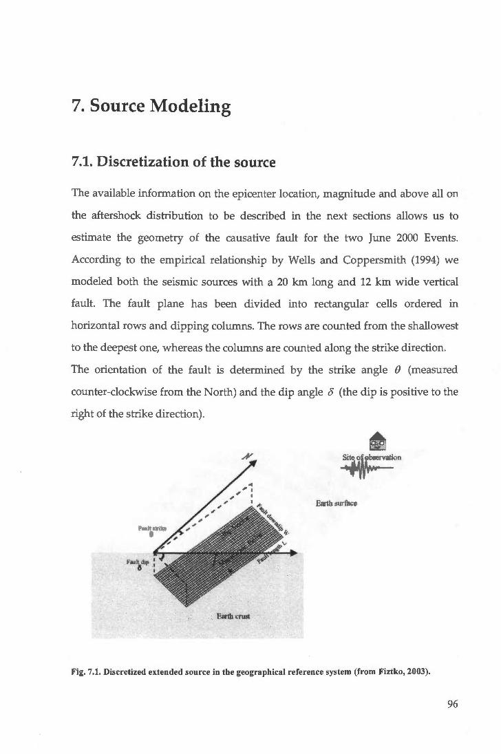
7. Source Modeling
7.1. Discretization of the source
The available information on the epicenter location, magnitude and above ali on
the aftershock distribution to be described in the next sections allows us to
estimate the geometry of the causative fault for the two June 2000 Events.
According to the empirica! relationship by Wells and Coppersmith (1994) we
modeled both the seismic sources with a 20 km long and 12 km wide vertical
fault. The fault piane has been divided into rectangular cells ordered in
horizontal rows and dipping columns. The rows are counted from the shallowest
to the deepest one, whereas the columns are counted along the strike direction.
The orientation of the fault is determined by the strike angle (} (measured
counter-clockwise from the North) and the dip angle 8 (the dip is positive to the
right of the strike direction).
00 -~o n
EaJtb surf..tee
Fig. 7.1. Discretized extended source in the geographical reference system (from Fiztko, 2003).
96

The origin of the reference system is defined with the geographic coordinates of
a point on the surface in the source proximity.
Usually the best choice is to keep as the reference position the upper left corner
of the rectangle modeling the rupturing surface. In this way the length and the
width of the fault's rectangular model are given by the number of grid cells in a
row and in a column, respectively, and the nucleation point, also expressed in
terms of grid cell coordinates, correspond to the hypocenter position.
Map view 64' 20'
64' 00'
63' 40'
* epicenter
Grid model of the fault piane along strike
Cross sectìon vìew toward dlrectlon 358.0"
.. ·I ·(-3.J! ·1 O 1, l'58
Fig. 7.2. Map view of the region (left) with the location of the stations (blue triangle) with to
respect the fault trace and the epicenter (red star). Grid model of the fault piane (right): the
reference position defines the geographic coordinates of the origin of a reference system with
respect to which the extended fault is parametrized (see text).
In the table below the geographical coordinates and all the parameters used in
the modeling of the two faults are reported.
Table 7.1. List of parameters used in the modeling the two faults. NP=nucleation point given
as celi number; h=depth of the hypocenter (in km); dip, strike and rake are given in degree.
97

7.2. Source time function modeling
Let we consider the source time function. The rupturing time of a cell is
calculated computing the delays corresponding to the arrivals at the cell of the
rupture propagation front from the source element chosen as hypocenter
(nucleation point), given a rupture propagation velocity in terms of a fraction of
the S-waves velocity. The rupturing times of all the cells are denoted as the
rupture propagation model.
Time Step
Rupture propagation Model
. ' ' ' ' ' ' 0.0 0.5 1.0 1.5 2.0 2.5 3.0 3.5 4.0 4.5 5.0
sec.
Moment Rate Function
8.00E.P.t
6.00Eo0,1
Tinte Step (s)
Fig. 7.3. Moment rate history. White cells are excluded from the source process andare not
allowed to sii p, according to the causality constraint and the rupture propagation model.
98

The total source duration is discretized by taking a fixed time step (IDT) which is
chosen as an integer number of the sampling interval of the seismograms. In the
framework of this thesis the sampling interval both for the computation of the
synthetic seismograms and for the resampled data is fixed at about 0.1 sec
(0.09765625 sec exactly). The number of source time steps depends on the choice
of IDT ( e.g. IDT=5 means that the total duration of the source process is sampled
at about 0.5 sec.).
The rupture propagation is thus reconstructed by the order of the celis which are
aliowed to break when the rupture front reaches them.
At the first time step, due also to the causality constraint, only the celi in
correspondence to the nucleation point can break, afterwards the moment can be
released progressively over ali the celis reached by the fracture front at
successive time intervals IDT.
Table 7.2. Temporal characteristics of the two events.
The amount of slip (or moment release) at each celi is determined by the
inversion process. The moment release can be visualized in space and time (Fig.
7.3).
99

7.1. The Hestvatn-Fault.
The IMO determined origin time of the June 21 earthquake is 00:51:46.95 GMT;
the hypocenter at 63.98°N, 20.71 ow, at a depth of 5.1 km. The USGS Rapid
Moment Tensor Solution gives a moment of M 0 = 5.2 x 10¹⁸ N m and preliminary
magnitudes by NEIC were mb=6.1 and Ms=6.6. South of the hypocenter,
64.05'
64'
63.95'
~111!1~~~~~~~~~- day 180200220 240 260 280 300 320 340 360
HESTVATN
Hypocenters a~~~r faultS'
2
10
12
14
63.90 63.95
:.
HESTVATN·
64.00 64.05
.: ··~:·· )"
p ..... ,.i; . :····' • .-... ~•-,c·•,•..;••
.;
2
4
10
12
14
16 +-----,--=--____,...--:.__,------r----'- 16
63.9'
-20.8 ' -20.7' -20.65' -20.8' -20.75' -20.7' -20.65'
Fig. 7.4. Maps views (left) and vertical cross section along strike (right) of the J21 Hestvatn
fault. The aftershocks (colour coded for different lime periods) delineate an approximately
16.5 km long fault, with an overall strike of N179° A and a di p (88°) to the west. The width of
the fault at the northern end is roughly 6km, increasing to 9km at the south end. The activity is
concentrated at the southern end and along the bottom of the fault (from Sigurlaug
Hjaltadottir, personal communication).
100

aftershocks are evenly distributed over the fault. North of the hypocenter the
activity is more sparse and mostly concentrated near the fault bottom. In the
interim between the two main shocks, seismic activity was mainly along the
bottom below the hypocenter, and along a conjugate fault (where surface rupture
was observed) extending westwards from the main fault. During the first 24
hours aftershocks are distributed over the entire fault up to about l km depth.
After that, activity concentrates along the bottom and through the whole depth
range at the southem end, where it is continuous throughout the year. South of
64°N the fault is continuous and quite linear, but steps westward at the bottom
under lake Hestvuan.
At shaliower depths the sparse activity north of the hypocenter shifts even more
westwards, towards the observed surface rupture. At the location of the mapped
conjugate rupture, the earthquake distribution is denser and extends a bit out to
the west. At the southern end of the fault a second set of conjugate faults is also
observed over a wide depth range. At the Southem margin the faults breaks up
into many smali fault sections of 1-2 km dimension and varying strike.
7.4. 21 June Event: summary of the inversion cases treated
Ali the inversion cases have been done using the causality constraint (with the
rupture velocity fixed), the moment constraint (i.e. total moment fixed) and
imposing that the moment can be released more than once (i.e. in successive time
steps) after the celi breaks. After fixing the geometrica! dimensions of the fault
(20 km x 12 km) we considered two fault's models by varying only the
dimensions of the grid celi (x-step) and consequently the number of celis along
strike (nx), along dip (nh) and the nucleation celi (NP). IDT is the other
101

parameter we tested. The number of the source time function time step and, as
the result, the number of equations (nu) and the number of unknowns (nv) in the
inversion problem depend on the choice of IDT.
Table 7.3. Summary of the inversion cases treated. See text for the full description.
According to the linear programming approach discussed in Chap. 5, we have to
minimize the vector of the residuals ( r = b- Ax ). W e define the fit as the function
fit = ~]x;colj; -coli; 1, where xi are the inverted slip rates, coli i are the real data,
colh are the synthetics computed from contributing grids.
The misfit is defined in the 11 sense as the ratio of the mean absolute error of fit
to the mean absolute amplitude of the data (Das and Kostrov 1990):
1 "ls; -r;l 11 -errar =-L.... l l , w h ere si are the values of the calculated synthetic nu r;
seismograms and ri those of the real ones, nu is the number of sampled
considered, i.e. the number of equations. Similarly, the misfit in the 12 sense
would be the ratio of the rms error of fit to the rms amplitude of the data
12 -errar=
102

In Table 7.3. are reported all the cases treated for the inversion of strong rnotion
data we have perforrned. Selected cases are discussed in detail below.
Case 1: Ml_IDT3
The first case we consider is M1 with IDT=3. This case correspond to a rupture
that spreads over the 20 krn long and 12 krn wide fault in 22 tirne steps with a
rupture velocity of v, = 0.7v5 •
21 June 2000 Ml_IDT3
o 1 2 3 4 5 6 7 8 9 10 o 1 2 3 4 5 6 7 8 9 10 o o o o
2
3
4
5
6 0123456 South
1 1
2 2
3 3
4 4
5 5
6 7 8 9 10
North
6 o 1 2 3 4 5 6 7 South
o 5000 1 0000 15000 20000 25000 30000
1 0"20 dyne*cm
8 9 10
North
2
3
4
5
6
Fig. 7.5. Moment distribution. Left: discrete representation of the moment release for each grid
celi. Right: Contour ma p of the total moment release.
The dirnension of the square cells is 2 krn and as the result the nurnber of cells
along strike is 10 and the nurnber of cells along dip is 6. The linear systern has
827 unknowns and 1008 equations. In the testing phase we use only the vertical
cornponent of the accelerograrns. Figure 7.5. shows the rnornent distribution
obtained over the fault. The rnaxirnurn is concentrated at the bottorn in the
southern part of the fault with a second release at a depth of 6 krn in the centrai
part of it. The Sirnplex Algorithrn cornpleted the rninirnization (fit ok in Table
7.3.). Even if the rnisfit is not perfect, being z1 = 0.6, the waveforrn fit shown in
Fig. 7.6. rnay be considered quite good for real data (in particular for severa!
103

stations such as Irafoss-Hydroelectric Power Station, Kaldarholt, Ljosafoss
Hydroelectric Power Station, Minni-Nupur).
21 June 2000, Model Ml_IDT3
~ ·10
~ -j--- -,-- ,. ···-·····- ,-- T --·-·,.----; ---- ,-·-··-_,.----, ... " " 20 ,
" 20 'l A'\:jbj..,...OOit ' :\
I o .r. 1
~ ~
~
TIITI9(s)
· -~ ~.fqjj~Hu;e ' j ·' ~ -1 f\.r· A ' l {' ~
~ o -:Ì 'ni '·l V l , ' ' \, !l \ofv·Y<: v-----~ -~ \l v
l v ~ ·-t----,--,---··t---T--------T----.-------r·---,----~
o <4 8 12 16 20 Tin'O{O
20
-3) -.. 4 r-··--·r··--·-·-r·······-.,--- r--···-·-··r -· -r .. -·-··-·r--·l . ~
i -120 -r-.- -~-.----- ., -,-,--- , --1-~
4 8 12 16 ~
Tlme(s)
,
Fig. 7.6. Comparison for each station between the real (thin black solid line) and the synthetics
(thick coloured solid line) accelerograms.
This first result was considered not satisfactory because the bottom concentration
of moment release was not in agreement with the results obtained inverting
geodetic data, nor with the observations that notice surface fractures.
104

Case 2: Ml_IDT5
This case is equivalent to the previous one except for the value of IDT; the linear
systern has now 553 unknowns and 1008 equations. IDT5 rneans that the source
21 June 2000 Ml_IDT5
o 2 3 4 5 6 7 8 9 10 o 2 3 4 5 6 7 8 9 10 o o o o
2 2 2 2
3 3 3 3
4 4 4 4
5 5 5 5
6 6 6 6 o 1 2 3 4 5 6 7 8 9 10 o 1 2 3 4 5 6 7 8 9 10
South North South North
o 5000 1 0000 15000 20000 25000 30000
1 Q/\20 dyne*cm
v .. ,---~~--....,.-----r-r-i
o 4 8 12 16 Xl
a -, Ragjanart-dt
_, l ., T- , ..... _1_ -,· -,
~ ~--.--,-~--,-,--,-.-, o 4 • "' • ] 1-f.e<gen:i-Rairemrt~""''
4 -- --~ ~ j li 'n·, l ~ ~ , <~~'v \.i',r·.p,_·'r-----
.a -l----,----i--··r·-·-r··----r - T-------,-r---,--1 o 4 8 12 16 ~
l irTejs) 10 ! lr<i:ml-l,<:loele:lricR:Ma-9alon
5 -l {\_ ~ o i - 1 ~ ~ ·-
10 ~ _, 5 -~ ---- -,----·····-r··---.,---~-----,-!--------,.-----T--··········r ···········1
o 4 8 12 16 20 15 "l f<ad:rtdt lin111(s)
l ' 10 -~
t : ~ ~ _, _J
· 10 j _,5 -t-····- ···r--·····t··---.. -·T····-·····-,····· r ·····- ~ ........... r
" 16 20 Tirre(S)
Fig. 7.7. Same as captions of Fig. 7.5. and 7.6.
12 16 20
' J Mm-I\4>J
i .. - / .. '
~ :J· . [i
•12 ....... ..,.--,-,-,--..,-- 1---.---,-r---1
SeJfa&(lty f{il 16 "'
1~
16 "'
105

time function is sampled at 0.5 sec and consequently the rupture process is
accomplished in 14 time steps. The fit is more or less the same plotted in Fig.7.6.
and the moment release is stili in the southern bottom corner of the fault (Fig.
7.7).
Case3: M2
In this case the dimension of the square celi is 1.5 km fora 21 km long and 12 km
wide fault. The number of cells along strike is 14 and the number of cells along
dip is 8. With IDT=3 the linear system has 1515 unknowns and 1255 equations.
The most part of the moment release doesn't change position and is stili
concentrated in the southem part of the fault even if we have also a release at
about 6 km depth.
i o
~ -5
-10
-15 -+---~~~· ~~~--.------,----.-- l
12 16 2l
.a ~ i
l -12 - -~ r .......... ! l l
4 8 12 18 20
15 l<acHtdt Tirre(s)
10
-5
-10
-15
12 16 2l lime(s)
Fig. 7.8. A Zoom of the best fits obtained with M2_IDT3 and the location map of the station
where they are obtained. In black thin solid lines are plotted the real accelerograms and in red
thick solid line the calculated ones.
106

With a finer grid we obtained an improvement both of the Zl-misfit, being 0.59
and of the waveform fit both in the near stations and in the distant ones.
However the number of unknowns becomes larger as the number of cells
increase.
21 }une 2000 M2_IDT5
1 2 3 4 5 6 7 8 9 10 11 12
South North
o 1 2 3 4 5 6 7 8 9 10 11 12 13 14 o o
2 3
4
7
8 o 1 2
South
1
2 3
4
5
6
7
8 3 4 5 6 7 8 9 10 11 12 13 14
North
1 0000 20000 30000 40000
1 CY'20 dyne*cm
L _ __..,.,_;:, .~/ ~ _,
4 -<
L --!1
-4 -i
-a ---l----- --,-- -------T -----,-------T---,---,-4 e 12
~d-R!Iinmrt~1
10
~ o
~ ·5
-10
-10
16 .,
16 20
16 20
-15 --·-;--- -----~---T·-~"f-""1---,---··r-··-r---~
o 8 12 16 :l)
Tirref$1
I !l -5
-10
12 16 Time(s)
· · r--···-, ----,..-···-···,·-·····1 12 16
Time{s)
oo -] ~ Tirrefs) 12
.., J ! ._a_j .. li i ~ •' 'i 4) ! il
«l ·] 1
20 16
-120 -··+-··-····-T"·-··----1- ··r .......... T ··········r- ······r·-·-···l
a ' 12 18 20
lirre(s)
Fig. 7.9. Same as captions of Fig. 7.5. and 7.6.
107

It is important to underline at this point that in a unconstrained system Ax = b,
the number of equations should be greater or equal than the number of
unknowns. This is however not relevant to the present problem, as the imposed
constraints provide additional conditions. The positiveness constraint in some
sense is equal to an infinite number of additional equations.
With IDT=5 the system has 1024 unknowns and 1255 equations and for the first
time we have a less deep moment release with a stronger asperity at about 6 km
depth in the southem edge of the fault and another one more to the north (Fig.
7.9.) This result was again considered as provisional and hardly acceptable, also
because to north of the hypocenter our inversions hardly give any significative
moment release.
Case 4: Ml_IDT3_3c
To better constrain the moment distribution, both because the results obtained
using only the vertical component of the accelerograms were not exhaustive, and
for increasing the number of equations of our linear system, we decided to use
also the horizontal components of the records.
2
3
4 ..
5
South
21 June 2000 Ml_IDT3_3c
2 2
3 3
4 4
5 5
1 2 3 4 5 6 7 8 9
1 2 3 4 5 6 7 8 9 10
North South North
o 5000 1 0000 15000 20000 25000 30000
1 QA2Q dyne*cm
Fig. 7.10. Same as captions of Fig. 7.5.
108

In spite of several trials the Simplex Algorithm did not complete the
minimization for any of them. We found out that this was due to our erroneous
assumption that the longitudinal and transversal components as given in the
i
t s
i s
'W *"' -
t s
i
' s
s
N
• -[
Fig. 7.11. Orientation of the strong motion instruments (from Simon Olafsson, personal
communication).
109

ISESD database were related to the hypocenter. After talking with the colleagues
of the University of Iceland we realized that this was not true and after they
determined the orientation with respect to the North of the strong motion
instruments, we were finally able to rotate correctly the horizontal components.
This case is equal to M1_IDT3. Most of the moment release is concentrated in the
centrai part of the fault with a stronger asperity at a depth about 4-5 km in the
south and another smaller one in the north at about 6-7 km depth. This
distribution seems to be more reasonable compared with the result obtained by
the inversion of geodetic data (Pedersen et al. 2003) as we will see in the next case
(Fig. 7.18.)
M1_1DT3_3c Z-component
111YB($)
8 Mnri-Nt.ps
Tin'U(s)
Fig. 7.12. Same as captions of Fig. 7.6.
The waveform fit (Fig. 7.12.) is not as good as in the previous cases, but the
number of inverted records is triple now. However, for the Z-component the fit
is particularly appreciable at stations Burfell-Hydroelectric Power Station,
Irafoss-Hydroelectric Power Station, Kaldarholt, Minni-Nupur.
110

As regards the NS-components, the comparison is quite good for Ljosafoss
Hydroelectric Power Station, Minni-Nupur. In generai, the amplitude of the
calculated signals is less than that of the re al ones. The EW -components are
better reproduced at the station located east of the epicenter like Burfell
Hydroelectric Power Station, Kaldarholt, Minni-Nupur (Fig. 7.13.).
Tloe('s)
TIITift(s)
lim.t(s)
Fig. 7.13. Same as captions of Fig. 7.6.
Case 5: Ml_R
M1_1DT3_3c EW-component
: ,~MI'JU4>-r:' l : ·.· .. · . ',; ;, :,, '. ' .
~::·······~~
M1_1DT3_3c NS-component
Selbs&Oty Hall l
When discussing the results with collegues of the University of Iceland, we noted
that our fault' s m od el was located a few kilometers to much towards north with
111

respect to the relocated aftershock distribution. In particular our reference
position (celll, l) seemed to be located only 5 km south of the center of the fault
(and of the nucleation point). Also the maximum moment release of our
preliminary models occurred beneath the center of the fault and also toward its
southern tip pointing to the fact that the fault should be extended towards the
South. Based on the relocated events, (Hjaltadottir, personal communication),
and on a revised fault' s extension and nucleation point we ha ve moved our fault
model by 5 km to the South 5 km with the nucleation point location being now
near the center of the fault.
21 June 2000 Ml_R
o 1 2 3 4 5 6 7 8 9 10 o 1 2 3 4 5 6 7 8 9 10 o o o o
2 2 2 2
3 3 3 3
4 4 4 4
5 5 5 5
6 6 6 6 o 1 2 3 4 5 6 7 8 9 10 o 1 2 3 4 5 6 7 8 9 10
South North South North
o 1 0000 20000 30000
1 0"20 dyne*cm
Fig. 7.14. Same as captions of Fig. 7.5.
The result for this model, called Ml_R, shows that the maximum moment release
is located at a depth of about 7 km, about 2 km south of the hypocenter,
coinciding with the intersection of the main fault and the westward extending
conjugate fault (where surface rupture was observed). Another significant
moment release follows approximately the distribution of the aftershocks along
the bottom of the fault, increasing in depth from 7 km at the northern end of the
fault, to 11 km just south of the nucleation point. Two additional strong maxima
are located near the surface. The smaller one is located 4km south of the
112

nucleation point, the stronger is 2 km north of it, approximately at the end of the
vertical section of the fault. The waveform fit is shown in Figs.7.15, 7.16, 7.17. For
the Z-component the fit is particularly satisfactory at the locations Burfell
Hydroelectric Power Station, Irafoss-Hydroelectric Power Station, Kaldarholt,
Minni-Nupur.
21 June 2000, Model M1_R, Z-component
T1me(s) Time(s)
' Hveragerdi-Retirement House 10 ' lrafoss-Hydroelectric Power Station
-15
12 16 20 12 16 lime(&) T ime( al
Kaldarholt Ljosafoss-Hydroelectric Power Station
I o
l -5
16 20 Time(s) Timo(s}
12 Selfoss-City Hall
Minni-Nupur
l 4
·8
Tìmo{s) 12 16 20 Time(s)
80 Thjorsartun
40
I o .~,...___ _____ _
~
20 nma(sì
Fig. 7.15. Same as captions of Fig. 7.6.
113

As regards the NS-components, the comparison is rather good for Burfell
Hydroelectric Power Station, Irafoss-Hydroelectric Power Station, Ljosafoss
Hydroelectric Power Station. The amplitude of the calculated signals is though
somehow smaller than that of the observed ones, particularly for Minni-Nupur,
Kaldarholt, Hveragerdi-Retirement House and Selfoss-City Hall.
The obtained EW-components are better reproduced at locations Burfell
Hydroelectric Power Station, Kaldarholt, Minni-Nupur, while the waveform fit is
less satisfactory at Ljosafoss-Hydroelectric Power Station, Hveragerdi
Retirement House and Flagbjarnaholt.
21 June 2000, Model M1_R, NS-component
12 · Burfeii-Hydroeleclric Power Slation 1° Flagbjamarholt !_
I ~
-4
f o
i -5
-8 -10
-12 -15
10 15 20 25 12 16 20 Time(s)
30 Hveragerd,I-Retirement House 20 lrafoss-Hydroel_eclric Power Slation
2() 10
I 10
~ o l -10
-20 --10
-30
-20
12 16 20 Tfme{s) 12 16 20
Time(s) 2() · Kaldarholl 40 Ljosafoss-Hydroeleclric Power Station
10 l: 20
f o
i -10 i
-20
12 16 20 12 16 20 Time(s) Tìme(s)
Minni-Nupur 30 Seifoss-City Hall
l
10 20
I 10
~ -10
-10
-20 -20 20 16
12 16 20 Time(s)
Time(s)
Fig. 7.16. Same as captions of Fig. 7.6.
114

21 June 2000, Model M1 _R, EW-component
···-: Burfe ii-Hydroelectrlc Power Station
·• Tlm11(s)
20 ···: Hver~gerd i-Retirement House
\
-40 _J_ ···r··L·····r ·-----·r·------0
8 ····; Minni-Nupur
'
-8 ·-i
i
Timo( l )
Time(s) " l
"
- 12 ....4--...-.-- , -~--~---~, ~.--,---...-l·--~---1 o 4 s 12 18 20
nme(•J
Fig. 7.17. Same as captions of Fig. 7.6.
.................. , ... _ ......... r-··-··-···-r·· ------, ......... , ..... _ .. ____ ì
" Tln101(!1J
30 "l lrafoaa-Hyd toelecltic Power Sta\ion
20 ~ f\
l ·: j ' -10 :1
20 -1 -)0 -+·----r-----
Tlmt(t)
~o - - --~ ljosafoss-Hydroelectric Power Slation
l !
~ ,: ~~- ,1\,,A , J li .
: l---T~-.------,-,- .. -, -T-~ " Tlm•(•)
•o j Selfoss-City Ha ll
l 20 ~
T Ime( Il
Far a better comparison with the results obtained with the geodetic data
inversion we have transformed the seismic moment into slip. In the relation
Mo = 11DA, where J1 is the shear modulus, D is the average slip and A the total
area, we have chosen an average value of J1 = 300kbar . lf moment is converted to
displacement and account is taken of the increasing velocity with depth
(increasing shear modulus with depth), displacement at the surface increase
significantly, but this is rather questionable. In Fig. 7.18. the slip distribution
obtained from the Ml_R model is reported along with that obtained by geodetic
data inversion (we will call it G_model in the following considerations).
115
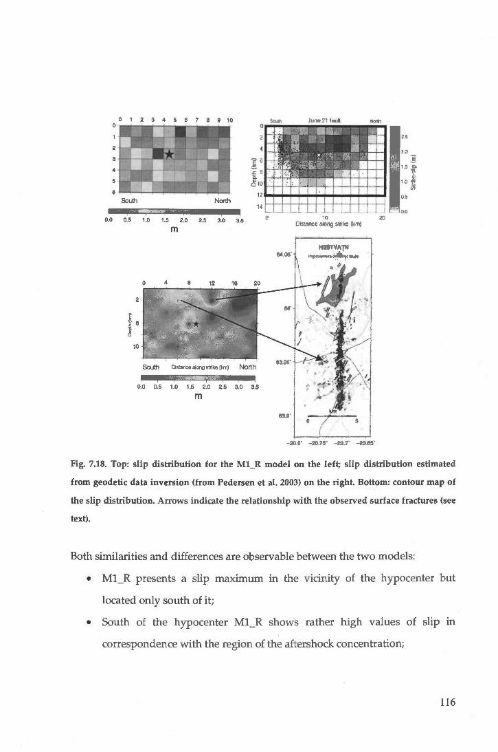
1 2 3 4 5 6 7 8 9 10
0.0 0.5 i
1.0
North
i i 1.5 2.0 2.5 3.0 3.5
m o 10 20
Oistance along s.trike (km)
HWTVA.TN 64.0ff Hlfl<>""'•<>~1rl-
-20.8' --20.75' -20.7' -2G.M '
Fig. 7.18. Top: slip distribution for the Ml_R model on the left; slip distribution estimated
from geodetic data inversion (from Pedersen et al. 2003) on the right. Bottom: contour map of
the slip distribution. Arrows indicate the relationship with the observed surface fractures (see
text).
Both similarities and differences are observable between the two models:
• Ml_R presents a slip maximum in the vicinity of the hypocenter but
located only south of it;
• South of the hypocenter Ml_R shows rather high values of slip in
correspondence with the region of the aftershock concentration;
116

• There is a lack of moment slip release north of the hypocenter for M1_R
model, while G_model has a maximum there;
• M1_R slip maxima near the fault's surface are m agreement with the
observed surface fractures, one north and one south of the epicenter.
These considerations based also on the fruitful exchange of data with the
University of Iceland and discussions with colleagues regarding the
observations, the accuracy of the fault's model and position, lead us to consider
M1_R as our best inversion result. This is also confirmed by the achieved value of
fit and misfit.
Case 6: Ml_Dip
According to the aftershocks distribution shown in Fig.7.1 one can notice that
north of the hypocenter the Hestvatn Fault seems to increase its dip: the bottom
part of the fault continue with the same direction as the vertical fault, the upper
part is evidenced by aftershocks located more to the west giving a dip of about
77° East. The intersection of the dipping segment with the surface, approximately
matches the mapped surface ruptures west of the lake Hestvatn.
In this inversion case we describe the sequence of }21 Event taking into account a
fault with a different dip in its northem part. We considered a first vertical fault
16 km long and 12 km depth (8 cells along strike and 6 along di p), with the same
nucleation cell (5, 3) as that of the M1_R model (in correspondence of the
earthquake hypocenter). A second fault has been taken 8 km long and 12 km
depth dipping 77° and overlapping the first one for the first 4 km along strike. In
this way the final fault had the same dimension of M1 fault model (20 km x 12
km). The rupture process spread over the composite fault with a rupture velocity
117

vr=0.7vs starting in the first fault and continuing in the second from the
conjunction celi between the two faults.
21 June 2000 Ml_IDT3_Dip
o 1 2 3 4 5 6 7 8 9 10 o 1 2 3 4 5 6 7 8 9 10
6 6 o o
5 5
4 4 2 2
3 3 3 3
2 2 4 4
5 5
o o 6 6 o 1 2 3 4 5 6 7 8 9 10 o 1 2 3 4 5 6 7 8 9 10
South North South North ''*
o 5000 1 0000 15000 20000 25000 30000
1 0"20 dyne*cm
Fig. 7.19. Same as captions of Fig. 7.5.
The moment distribution obtained is consistent with that obtained for Ml_R:
• The maximum is released at a depth of about 6km slightly south of the
hypocenter even if Ml_Dip presents a prolongation of moment release
toward the southern bottom corner of the fault and below the hypocenter;
• Ml_Dip gives again the two additional maxima located near the surface
in correspondence of the surface fractures, even if with smaller slip;
• In the Northern part of the fault Ml_dip does not present any important
moment release, in agreement with the Ml_R results.
118

7.5. The Holt-Fault.
According to the Icelandic Meteorologica! Office (IMO), the origin time of the
June 17 earthquake is 15:40:40.94GMT, the hypocenter is at 63.97°N, 20.37°W, at a
depth of 6.3 km. The USGS Rapid Moment Tensor Solution proposed a nodal
piane striking N4°E and dipping 84° to the East. The moment calculated by
USGS is M 0 = 6.0 x l 018 N m, assuming a best-fitting double-couple solution. The
preliminary magnitudes estimated by the National Earthquake Information
Center (NEIC) in USA were mb=5.7 and Ms=6.6. The study of the spatial
distribution of the aftershocks leads to some considerations (Fig.7.20.).
Aftershocks occur mainly in two vertical bands edges of the fault and along a
band a t depth (fault' s bottom), as well as in the fault center, below the
hypocenter. During the first 24 hours aftershocks are distributed over the entire
fault, after that, activity concentrates along the bands (fault margins), mostly
below 3 km. The overall strike of the fault is about 7 degrees and the fault is near
vertical, but it is composed of many smaller patches, with differing strikes.
Above 8 km depth the aftershocks display a rather discontinuous pattern
composed of three main patches. The activity delineates a very planar centrai
patch, which is active throughout the year. Its strike (about 11 degrees) is slightly
to the east of the overall strike of the fault. The overall dip of the fault is nearly
vertical. Activity on the northern patch is confined to its northern edge, where it
is composed of a few short patches mostly with a northerly strike. The southern
patch is more continuous and bends westwards with decreasing latitude. At the
southern tip the fault jumps half a kilometer to the west and continues on an
about 2 km long segment.
119

·~~~~·····-==··day 180200220240260280300320340360
:r
10
14 - 14
HOLT 16+-----.-------,--'---.------,---------l.. 16
63.9' km km
o 5 o 5
- 20.45' -20.4' -20.35' -20.45' -20.4' -20.35'
Fig. 7.20. Maps views (left) and vertical cross section along strike (right) of the Jl7 Holt-fault.
The aftershocks (colour coded for different time periods) define approximately an 11.5 km
long fault, with an overall strike of N197°, dipping slightly to the west. The fault width is 10
km, with the activity concentrated at the edges and on the center of the patch, where the
hypocenter of the main event is located (star). The event distribution at the bottom is
somewhat smeared in the E-W direction (see vertical cross section along strike) and dips
slightly to the east. The smaller star indicates the second Holt event (M=S) occurred 2 minutes
after the main event on June 17th, just west of the southern end of the Holt fault (from
Sigurlaug Hjaltadottir, personal communication).
W est of the southem edge a few small faults were also activated. Below 8 km the
aftershocks define a continuous fault, but with kinks at the intersection of the
main patches above. North of the center patch the bottom appears to be
composed of a few smaller en echelon faults and then breaks up into separate
parallel branches farther north. Activity on the southem part, on the other end,
120

appears to be continuous and more linear, bending slightly westward towards
the southern end.
7.6. The 17 June 2000 Event.
The sequence of the tests made for the 17 June 2000 Event is more or less the
same as for the 21 June 2000 one (Table 7.4.). Selected cases are discussed in
detail below.
Event Mode l n x nh x-step di p strike rake NP ldt nu(eq.) nv (unk.) 11-err 12-err fit Comments
M1 IDT3 10 6 2 87 4 196 6,3 3 2021 827 1.4 1.3 no 1.8!
M2 IDT3 14 8 1.5 87 4 196 84 3 2021 1513 1.1 0.97 no 1.5
M2 IDT5 14 8 1.5 87 4 196 84 5 2021 1022 5.4 6.4 no 7.1
M1 IDT3 7s 10 6 2 87 4 196 63 3 850 827 0.75 0.7 no 1.51 7 statlons 1 Os
M2 IDT5 7s 14 8 1.5 87 4 196 8,4 5 1050 1022 0.51 0.5 ok 0.9!
M1 5s 3C 10 6 2 87 4 196 6,3 3 1635 827 0.78 0.87 ok 3.58 5 nearest sta, 3-components
M1 5s 3C IDT5 10 6 2 87 4 196 6,3 5 1635 553 0.83 0.89 ok 3.8!
M1 R 10 6 2 87 4 196 6,3 3 1635 827 0.72 0.84 ok 3.3 fault relocatlon
Table 7.4. Summary ofthe case treated. See caption table 7.1.
We first selected 15 sec of duration of the accelerograms for inversion, without
realizing that part of some signals were contaminated by the triggered event in
the Reykjanes peninsula. For this reason our inversions were not successful: the
Simplex Algorith!TI did not reach the minimum (fit NO in table 7.4.) and did not
complete the procedure (e.g. M1_IDT3, M2_IDT3, M2_IDT5). Moreover, the
results produced an unreasonable maximum of moment release in the near
surface part of the fault. W e realized that this situation was due to a second event
occurred very dose to the main one, about 5 km to the west, near the
Hveragerdi-Retirement House station.
121

Case 1: M2_IDT5_7s.
To avoid the influence of the second event in our inversions we did not use data
from Hveragerdi-Retirement House station and from the more distant stations.
Moreover we reduced the part of the signals to be inverted to the first 10 sec. In
17 June 2000 M2_7s_IDT5
o 1 2 3 4 5 6 7 8 9 10 11 12 13 14 o o
8 8 o 1 2 3 4 5 6 7 8 9 10 11 12 13 14
South North
o 1 2 3 4 5 6 7 8 9 10 11 12 13 14 o o
2
3
4
5
6
7
1
2 3
4
5
6
7
8 8 o 1 2 3 4 5 6 7 8 9 10 11 12 13 14 South North
o 1 0000 20000 30000 40000
1 QA20 dyne*cm
"" . i Aa;tjaratdt l i
"' '
-t ···· ·---; o
------r·--··-·----, .. ·--·--····-T 8
'TirTB(S)
8 llme(s)
Tlmll{~
16
.. .,- - -,- l 12 16
Fig. 7.21. Same as captions of Fig. 7.5. and 7.6.
15 ..i Mrri-N..p.r
10 -----1
{ o ____ : :[
-5
-10
-15 •
·2
12
12 Time(s)
16
122

this case we used M2 as fault modei (see J21 fault description), IDT=5 and data
from oniy 7 stations. The assumed rupture veiocity is vr=0.7vs, the totai source
process is described in 22 time steps, the number of cells aiong strike is 14 and
the number of cells aiong dip is 8. The linear system has 1050 equations and 1022
unknowns. We used oniy the verticai component of the acceierograms in this
inversion.
The moment siip distribution obtained was more realistic: it is concentrated in
the centrai upper part of the fault and spread across two main asperities, with a
stronger one in the northem part of the fault at a depth about 6 km.
The waveform fit is particuiarly good for the dose by stations of Fiagbjamarholt,
Kaidarhoit, Minni-Nupur with a /1 -misfit equai to 0.51. waveforms at more
distant stations are not modelled so well.
Case 2: M1_5s_3c.
Aiso for the 17 June 2000 event, we made an inversion using alle three
components of the acceierograms for the M1 fault model. IDT=3, the number of
cells aiong strike is 10, the number of cells aiong dip is 6, the equations are 1635
and the unknowns are 827. In this case we invert the first 10 sec of the signais of
the 5 nearest stations.
The moment slip is concentrated in the centrai part of the fault with a stronger
asperity at a depth of 7-8 km under the hypocenter and another 6-7 km deep one
south of the hypocenter. The waveform fit is quite good for the verticai
component in particuiar for Burfell-Hydroeiectric Power Station, Fiagbjamaholt
and Kaidarhoit, while the horizontai components are better reproduce for Minni
Nupur and Selfoss-City Hall.
123

17 June 2000 M1_5s_3c
o 2 3 4 5 6 7 8 9 10 o 2 3 4 o o o
2 2 2
3 3 3
4 4 4
5 5 5
6 6 6 o 1 2 3 4 5 6 7 8 9 10 o 1 2 3 4 South North South
o 10000 20000 30000 40000
1 QA2Q dyne*cm
Z-component EW-component "a..ra~-S;jm
{ 1 o
,., _ ~
{ -+--·'· - • l ~ , lv .
l
. " Timi( si
/W'\tl .. ...-- t o
i. -10
.... r···--r--I
' -30 -- ··-----r---r-~- T----r---· .. .,--------
8 " """'~ '"'"
8 " .
Tlfl'll{t) Timi( l)
Fig. 7.22. Sarne as captions of Fig. 7.5 and 7.6.
5
5
10 ~··
~ -l~~ o
6 7 8 9 10 o
2
3
4
5
6 6 7 8 9 10
North
NS-component
8 T~t) "
.---~-.-~---~---~
8 T ome( t)
-30 -- ···-·-----,----···r·-·--,---r--...-----·T"---.---0 8 12
"""'"
. " ~ ... -!~-~-..--!--~,-~-..-, -~ . " -
124

Case 3: M1_3c_R.
Accordingly with the re-analysis of the aftershock distribution (Hjaltad6ttir,
personal communication), we slightly relocated the fault also for the J17 event
shifting it to the south according to the suggestions proposed by the colleagues
of the University of Iceland.
The result for M1_R shows that most of the moment is released on the centrai
patch, with a peak below and south of the hypocenter, extending about 8 km
along the fault and down to about 9 km depth near the center. A second
maximum is located at shallow depth (3 km) roughly 1 km south of the southem
edge of the fault. Two additional peaks in moment are also obtained near the
surface, (1 km depth), one at the northern margin of the fault and the other just
south of the fault center.
17 June 2000 M1_3c_R
o 1 2 3 4 5 6 7 8 9 10 o 1 2 3 4 5 6 7 8 9 10 o o o ' o
2 2 2 2
3 3 3 3
4 4 4 4
5 5 5 5
6 6 6 6 o 1 2 3 4 5 6 7 8 9 10 o 1 2 3 4 5 6 7 8 9 10
South North South North
o 1 0000 . 20000 30000 40000
1 0"20 dyne*cm
Fig. 7.23. Same as captions of Fig. 7.5.
In Flagbjamaholt and Kaldarholt stations even if the waveform amplitude
calculated is somewhat smaller than the real one, the fit is satisfactory for the Z
component. As regards the horizontal components, the EW-components are
better reproduced than the NS-ones, except at Flagbjamaholt station.
125

" i 10 l
l
l • l
l o ! ~ ., l
·10 1
-15 · 4
~ : ·10
8 Till'e{s)
Mmi-Nupur
Tirro(S)
Burfeii-Hydroe!edric Po.wr Station
Tonw(S) a
' Tome(s)
17 June 2000, M1_3c_R, Z-component
40 .. Aagbj"'""""'t l
·20 ··
-6 !...·--··-·-···-···
" lime( s.)
17 June 2000, M1_3c_R, Z-component
TorM(s)
1 Selfoss-Oly Hall
10
-10 •
-15 ···:! . ~' ..
17 June 2000, M1_3c_R, Z-component
lime(s)
' Tune(s)
Fig. 7.24. Same as captions of Fig. 7.6.
JO Kaldartdt
Tlnn{B)
126

In Fig.7.25 we show the comparison between our Ml_R model slip distribution
and that obtained by Pedersen et al., 2003 (we will call it G_model in the
following considerations ).
2
3
4
5
6
0.0
1 2 3 4 5 6 7 8 9 10
South North
0.5 1.0 1.5 2.0 2.5 3.0
m
0.0 0.5 1.0 1.5 2.0 2.5 3.0 3.5
m
Fig. 7.25. Same as captions of Fig. 7.18.
Analysing the results we can say:
Nonh
2.5
2.0
$ 1 .5 a.
'Bi
"' 1.0 "" ~ 0 .5
0.0 20
km
o
-20.45' -20.4' - 20.35'
• Ml_R reveals a moment slip distribution below the hypocenter extending
above depths of 9-10 km in the south to depths of about 6 km in the north
127

in correspondence of the lack of aftershock concentration. The G_model
has a small moment release in this area;
• The second maximum in the Ml_R model is about 3 km deep and is in
agreement with the southemmost part of the asperity in the G_model;
• Some secondary near-surface maximum above the hypocenter correlate
also well with both surface faulting and the G-model high moment
release. On the other hand the northemmost isolated high-moment patch
in our model finds no such correspondence.
• The additional peaks obtained near the surface, even if slightly shifted
toward north, are in agreement, in particular the first one above the
hypocenter, both with the G_model and the observed surface fractures.
Also for the Jl7 Event we consider the results obtained using Ml_R fault model
our best solution of the linear programming problem.
128

8. Uncertainties in slip inversions and
synthetic tests.
8.1. lntroduction
The matrix inversion of seismic data for slip distribution on finite faults is based,
as we have seen, on the formulation of the representation theorem as a linear
inverse problem. The way the problem is posed and parameterized involves
significant and often subjective decision-making. This introduces severallevels of
uncertainty. One can say that there are two levels of uncertainty in a formalized
slip inversion. We can separate them in the method and parametric uncertainty.
The method uncertainty lays at the most fundamentallevel: it comes from the
fact that there is no unique way of constructing an inversion scheme that would
satisfy reasonable constraints imposed by both numerica! stability and physics.
Depending on which set of constraint is chosen and how it is applied the result
of inversion may dramatically change. Once the method has been defined, the
parametri c uncertainty begins to affect the results ( e.g. the variability of the
position and orientation of the fault, of the rupture velocity, etc.). It is defined as
the sensitivity of the results to a particular choice of the parameters fixed in the
inversion. To formalize the problem as a linear matrix inversion, we constrained
to fix the rupture propagation velocity, the fault geometry, the crustal structure,
and the duration of the source time function.
129

Sensitivity analyses were conducted by Das and Suhadolc (1996), Das et al.
(1996), and Saraò et al. (1998) using a similar Haskell-type rupture with both
uniform slip and simple inhomogeneous slip distribution, as their synthetic
models. They investigated: (l) the effect of incorrect assumption of the rupture
speed, fault geometry and crustal structure (Das and Suhadolc, 1996; Saraò et al.,
1998), (2) the effect of particular near-fault station distribution (Saraò et al., 1998);
(3) the effect of adding noise to synthetic data (Saraò et al., 1998).
The conclusions were rather pessimistic: the near-field stations geometry
virtually predetermined the resulting solution and adding extra stations could
sometimes even worsen it (Saraò et al., 1998); incomplete knowledge of crustal
structure could ruin the inversion so that no realistic part of the real fault was
recovered (Das and Suhadolc, 1996; Saraò et al., 1998); incorrect assumption
about the parameters or the addition of noise to the synthetic produced geologie
artefacts, such as non existing asperities, spurious fault inhomogeneity, or a
ghost rupture front (Das and Suhadolc, 1996).
A synthetic test that would truly mimic the inversion of a real earthquake's data
would be to carry out an inversion in which all assumed parameters are
perturbed from their true values and see whether this would stili allow a
reasonable slip recovery.
8.2. Synthetic tests.
The soundness of obtained slip inversion is best tested if the inversion results are
compared with the actual distribution of slip on the fault, which is impossible for
natural earthquakes. In the absence of the possibility to compare the inversion to
the true solution, the only way of testing the inverse algorithm is to apply it to
130

synthetic data obtained from the solution of a forward problem based on the
representation theorem.
For the synthetic tests in the framework of this thesis we fix all the source's
parameters (fault geometry, rupture speed, the crustal structure, and station' s
distribution) and we investigate the possible complexity of the slip distribution
on the fault's surface due to the parametrization of cells rupturing in space and
time.
Case A: We start first with a simple example. We calculate synthetic vertical
accelerograms corresponding in this case to a unilateral rupture that spreads
over a 4km x 4km fault in 30 time steps (nsource) with a rupture velocity of
vr = 0.7v5 breaking each cell only once. The dimension of the single cell is lkm x
lkm and the final moment distribution over the fault for this forward problem is
a chessboard type of distribution (Fig. 8.1). We used the fault mechanism
parameters and station distribution of the Jl7 event.
4x4 OnlyOnce ., .• , •• ""1•1
'•;[
11 MTO No-Moment Moment No moment Moment
nu 1393 1393 1393 1393 n v 16 16 233 233 fit YES YES YES NO
4.27602 4.27605 4.27636 4.27878 broken cells 16 16 47 34 delta 1.00E-09 1.00E-01 1.00E-25 0.1 EPS 1.00E-25 1.00E-35 1.00E-35 1.00E-35 nsource 30 30 30 30 sta 9 9 9 9 idt 1 1 1 1 su m x 79999.9 80000 80001.6 80000
Fig. 8.1. On the left is reproduced the chessboard moment distribution on the fault's surface.
Blue celi correspond to a value of 1*1016 Nm, orange celi to a value of 9*1016 Nm. In the table
on the right are reported ali the parameters used and the results obtained (see text).
131
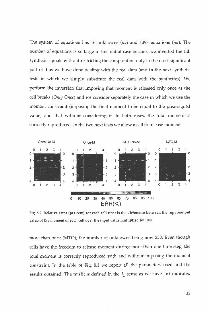
The system of equations has 16 unknowns (nv) and 1393 equations (nu) . The
number of equations is so large in this initial case because we inverted the full
synthetic signals without restricting the computation only to the most significant
part of it as we have done dealing with the real data (and in the next synthetic
tests in which we simply substitute the real data with the synthetics). We
perform the inversion first imposing that moment is released only once as the
cell breaks (Only Once) and we consider separately the case in which we use the
moment constraint (imposing the final moment to be equal to the preassigned
value) and that without considering it. In both cases, the total moment is
correctly reproduced. In the two next tests we allow a cell to release moment
Once-No-M Once-M MTO-No-M MTO-M
2 2 2 2 2 2 2 2
3 3 3 3 3 3 3 3
3 2 3 2 3 2 3
' ' i ~ ;;;p o 10 20 30 40 50 60 70 80 90 100
ERR(0/o) Fig. 8.2. Relative error (per cent) for each celi (that is the difference between the input-output
value of the moment of each celi over the input value multiplied by 100).
more than once (MTO), the number of unknowns being now 233. Even though
cells have the freedom to release moment during more than one time step, the
total moment is correctly reproduced with and without imposing the moment
constraint. In the table of Fig. 8.1 we report all the parameters used and the
results obtained. The misfit is defined in the Z1 sense as we have just indicated
132

1 is· -r·l (i.e.l1- errar= -I 1l l 1
); the case when the Sirnplex Algorithrn cornpletes nu ri
the cornputation and reaches the rninirnurn is noted as ''jit=YES"; sta is the
nurnber of stations, idt is the source tirne function tirne step, sumx is the value of
the total rnornent scaled by 1015 Nrn, delta is the pararneter to stop optirnization
when this value of relative rnisfit is reached, EPS is the protection frorn srnali
pivots (see Sirnplex procedure).
In order to see the level of accuracy with which the rnornent slip distribution is
reproduced by the inversion of synthetic data, we plot (Fig. 8.2) the relative errar
(per cent) for each celi (that is the difference between the input-output value of
the rnornent of each celi over the input value rnultiplied by 100). For this first
sirnple test the rnornent distribution is cornpletely reproduced within a 10%
error. Far the first three cases the errar is even within l%, while for the last case
we have a celi at the bottorn of the fault which is not perfectly reproduced (18%).
Case B: In order to establish the level of resolution of the rnornent distribution
over the fault we can obtain in the inversion, we consider three increasingly
detailed rnornent distributions in the forward problern.
5
4
3
2
Distribution 1 2 3 4 5 6 7 8 9
1 2 3 4 5 6 7 8 9
Distribution2 Distribution3 o 1 2 3 4 5 6 7 8 9 10 o 1 2 3 4 5 6 7 8 9 10
6 6 6 6
5 5
4 4
3 3
. 2 2
1 1
5
4
3
2
o o o o o 1 2 3 4 5 6 7 8 9 10 o 1 2 3 4 5 6 7 8 9 10
o 1 000 2000 3000 4000 5000 6000 7000 8000 9000
1 QA20 dyne*cm
Fig. 8.3. 3 moment distributions progressively (from l to 3) more detailed used as input in the
forward problem.
133

We calculate synthetic vertical accelerograms corresponding in this case to a
10km x 6km fault in 300 time steps with the usual rupture velocity (v, = 0.7vs ),
the dimension of the celi is 1km x 1km. We use again the fault mechanism
parameters and station distribution of the J17 event. The system of equations has
60 unknowns and 844 equations when we use the Only Once constraint, and
2033 unknowns when we use the MTO constraint.
Case Bl: Slip only once, no-moment constraint.
For this first subcase the first distribution is reproduced within a 10% error, for
the second distribution and in particular for the third one we can see that at the
bottom of the fault some cells are not perfectly reproduced. The red cells, one for
the second distribution and five for the third, are cells which didn't break during
the inversion (the value of the moment release on them is zero) an d consequently
have the maximum value of error (100%). Also the simplex algorithm of
inversion reached its value of misfit completing the computation only for the first
distribution (see table 8.1.)
Only Once No-Moment constraint
o 1 2 3 4 5 6 7 8 9 10 o 1 2 3 4 5 6 7 8 9 10 o 1 2 3 4 5 6 7 8 9
o o o o o 1 1 1 1
2 2 2 2 2 2
3 3 3 3 3
4 4 4 4 4 4
5 5 5 5 5
6 6 6 6 o 1 2 3 4 5 6 7 8 9 10 o 1 2 3 4 5 6 7 8 9 10 1 2 3 4 5 6 7 8 9
O 10 20 30 40 50 60 70 BO 90 100
ERR(%) Fig. 8.4. Case Bl: Sii p only once, no-moment constraint. Relative error per cent for each celi.
134
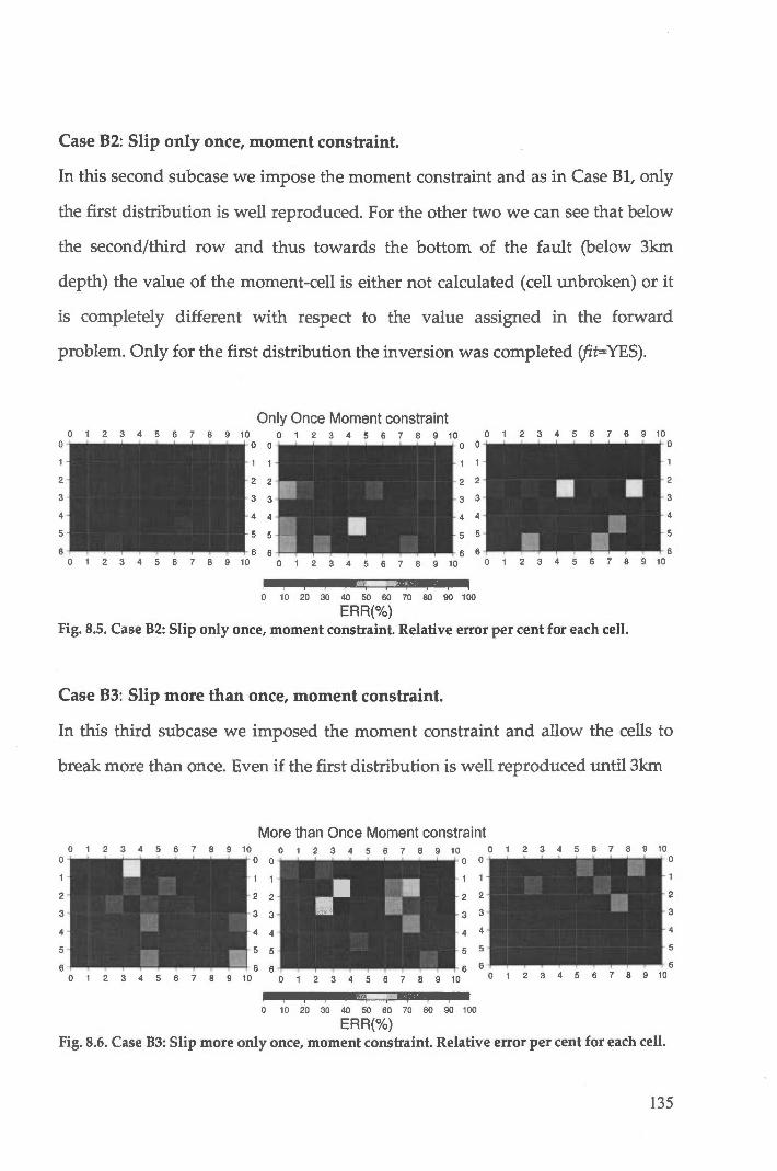
Case B2: Slip only once, moment constraint.
In this second subcase we impose the moment constraint and as in Case Bl, only
the first distribution is well reproduced. For the other two we can see that below
the second/third row and thus towards the bottom of the fault (below 3km
depth) the value of the moment-cell is either not calculated (celi unbroken) or it
is completely different with respect to the value assigned in the forward
problem. Only for the first distribution the inversion was completed (fit=YES).
Only Once Moment constraint 1 2 3 4 5 6 7 8 9 1 2 3 4 5 6 7 8 9 1 2 3 4 5 6 7 8 9
1 1 1 1
2 2 2 2 2 2
3 3 3 3 3
4 4 4 4 4
5 5 5 5 5
1 2 3 4 5 6 7 8 9 1 2 3 4 5 6 7 8 9 1 2 3 4 5 6 7 8 9
o 10 20 30 40 50 60 70 80 90 100
ERR(%) Fig. 8.5. Case B2: Sii p only once, moment constraint. Relative error per cent for each celi.
Case B3: Slip more than once, moment constraint.
In this third subcase we imposed the moment constraint and allow the cells to
break more than once. Even if the first distribution is well reproduced until 3km
More than Once Moment constraint 1 2 3 4 5 6 7 8 9 1 2 3 4 5 6 7 8 9
123456789 123456789
O 10 20 30 40 50 60 70 BO 90 100
ERR(%)
123456789
123456789
2
3
4
5
Fig. 8.6. Case B3: Sii p more only once, moment constraint. Relative error per cent for each celi.
135

depth, below the third row the result are very bad. The situation is even worse
for the other two distributions and, in particular, the third distribution in not
reproduced at ali. In ali three cases the inversion was not completed (fit=NO).
J17 Only Once -.n-o (1kmx1km) No-Moment Moment No moment Moment
nu 844 844 844 844 nv ;r 60 60 2033 2033 fit YES YES NO NO
2.71E-04 2.72E-03 0.7313 0.207583 broken cells 60 60 101 119 delta 1.00E-15 1.00E-14 0.1 0.1 EPS 1.00E-25 1.00E-35 1.00E-25 1.00E-25 nsource 300 300 300 300 sta 5 5 5 5 id t 1 1 1 1 sumx 300000.1 300000 496980 299898 nu 844 844 844 844 n v 60 60 2033 2033 fit NO NO NO NO
8.82E-02 9.16E-02 0.5319 0.208464 broken cells 59 50 108 105 delta 1.00E-10 1.00E-01 1.00E-01 1.00E-01 EPS 1.00E-25 1.00E-25 1.00E-25 1.00E-25 nsource 300 300 300 300 sta 5 5 5 5 id t 1 1 1 1 sumx 316021 316000 442044 316186
nu 844 844 844 844 n v 60 60 2033 2033 fit NO NO NO NO
0.102351 5.90E-02 0.5129 0.623703 broken cells 55 50 96 146 delta 1.00E-10 1.00E-01 0.1 0.1 EPS 1.00E-25 1.00E-35 1.00E-25 1.00E-25 nsource 300 300 300 300 sta 5 5 5 5 id t 1 1 1 1 su m x 302270 300000 370574 300000
Table 8.1. In the table are reported ali the parameters used and the results obtained (see text) for
Case B. From top to bottom in grey, blue and light blue are indicated the three distributions (1, 2, 3
see Fig. 8.3.) and from left to right the results obtained by imposing the different constraints.
Case C: In this case we use exactly the Jl7 event fault parameters. As
summarized in table 8.2, the fault' s dimensions are now 20km x 12km, the celi' s
size is 2km x 2km, the time steps are 66, idt=3, the rupture velocity is kept at
v, = 0.7vs, and we teste the three-moment distributions of Fig. 8.3. The system of
136
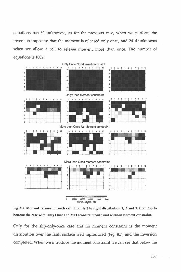
equations has 60 unknowns, as for the previous case, when we perform the
inversion imposing that the moment is released only once, and 2414 unknowns
when we allow a cell to release moment more than once. The number of
equations is 1002.
1 2 3 4 5 6 7 8 9 10
1 2 3 4 5 6 7 8 9 10
Only Once No-Moment constraint
Only Once Moment constraint
1 2 3 4 5 6 7 8 9 10
- l. • . • -.
More than Once No-Moment constraint
1 2 3 4 5 6 7 8 9 10 1 2 3 4 5 6 7 8 9 10
More !han Once Moment constraint 1 2 3 4 5 6 7 8 9 10 1234567 9 10
1 0000 20000 30000 40000 50000
1QI\20 dyne*cm
1 2 3 4 5 6 7 8 9 10
1 2 3 4 5 6 7 8 9 10
1 2 3 4 5 6 7 8 9 10
1 2 3 4 5 6 7 8 9 10
Fig. 8.7. Moment release for each celi. From left to right distribution l, 2 and 3; from top to
bottom: the case with Only Once and MTO constraint with and without moment constraint.
Only for the slip-only-once case and no moment constraint is the moment
distribution over the fault surface well reproduced (Fig. 8.7) and the inversion
completed. When we introduce the moment constraint we can see that below the
137

middle of the fault white cells ( cells which did not break and ha ve consequently
the value of the moment equal to zero) begin to appear. For the MTO case we can
notice that the moment distribution is not reproduced and the inversion not
completed.
Table 8.2. In the table are reported ali the parameters used and the results obtained (see text) for
Case C. From top to bottom in grey, blue and light blue are indicated the three distribution (1, 2, 3
from Fig. 8.3.) and from left to right the results obtained by imposing the different constraints.
Case D: W e have just underlined as in the framework of our linear programming
approach it is not fundamental that the number of equations is greater than or
138

equal to the number of unknowns. However, the principal reason for the not
very satisfactory results of the synthetic test in the Case C is due to the lack of
"artificial" data. I want to remind you that the number of equations comes from
the number of data points of the signal's window (real or synthetic) chosen for
the inversion. In case C (see Table 8.3) the equations are 1002 and the unknowns
are 2414. As a matter of fact, adding more data by introducing more "virtual
stations", the number of blank celis is considerably reduced. Thus it is quite
reasonable that the more are the available data, the better are the results of the
minimization procedure of the algorithm. With almost 4 times more stations, the
three distributions of Fig. 8.3 are almost recognizable (Fig. 8.8) even if stili not
perfectly. The number of equations in this case is 3247.
19 STA, More than Once Moment constraint
1 2 3 4 5 6 7 8 9 10
3
4
6
2
3
4
6
1 2 3 4 5 6 7 8 9 10
5
4
3
2
o
o 1 0000 20000 30000 40000 50000
1 0"20 dyne*cm
1 2 3 4 5 6 7 8 9 10
Fig. 8.8 Moment release for each celi for the case with 19 stations, MTO and moment
constraint. From left to right: distribution l, 2 and 3.
Another way to enlarge the number of equations, like we have done using real
data, is to use ali three components of the signals. In ali the previous synthetic
tests we used only the vertical components of the accelerograms. In the foliowing
case we reproduce exactly the J21 M1 fault model using also the horizontal
components. The number of equations is 4412 and the number of unknowns is
827. However, both in this case and in the previous one (Table 8.3) the simplex
139

2
3
4
6
9 STA, 3-components, More than Once Moment
1 2 3 4 5 6 7 8 9 10 1 2 3 4 5 6 7 8 9 10
o 1 0000 20000 30000 40000 50000
1 QA2Q dyne*cm
3
4
6
1 2 3 4 5 6 7 8 9 10
Fig. 8.9 Moment release for each celi for the case reproducing J21 Ml model with 9 stations, 3
components, MTO and moment constraint. From left to right distribution l, 2 and 3.
T ab. 8.4. In the table are reported ali the parameters used and the results obtained (see text) for Case
D. From top to bottom in grey, blue and light blue are indicated the three distribution (1, 2, 3 from
Fig. 8.3.).
140
algorithm completes the procedure of computation, but the convergence is
obtained too rapidly resulting in a relative big value of misfit.
Other tests are stili in progress in order to understand this apparently strange
behaviour of the Simplex procedure. Unfortunately, with a number of equations
progressively larger and larger the time of the computation grows considerably.
A first important, although somehow foreseeable, conclusion is that the
minimizing procedure we use in the inversion of strong motion data encounters
some difficulties as the dimension of the matrix associate to the linear system
grows in dimensions. However, the synthetic tests carried out for a linear
programming problem of the dimension equal to that of our real inverse
problem, (in terms of number of equations and constraints applied), shows that
the upper half part of the fault is well reproduced and that the use of ali
components of motion is crucial, especially when the number of station is
limited, to obtain reliable results.
This allows us to conclude that the obtained results with real data inversion can
be considered appreciable with a resolution of at least 3 km x 3km for the upper
half of the fault. This is particularly goodnews for the J21 event, since most of the
moment release has been obtained near the surface.
141
9. Strong ground motion scenarios
9.1. Introduction
The study of strong ground motion, earthquake hazard and risk plays an
important role in seismology and in the sustainable development of economies
and societies. Hazard analysis requires the characterization of the seismic sources
that can be expected to affect a selected piace in terms of locations, magnitudes,
and frequency of occurrence of potentially damaging earthquakes. Knowledge of
the attenuation of ground motion or seismic intensity with distance from the
source to the site, integrated whenever possible with realistic modeling of
seismic wave propagation, and knowledge of the local geology for site-specific
assessment will promote this analysis to a large extent. Using the hazard
estimates produced by seismology, risk analysis yields probabilistic estimates of
the expected losses of property and lives from earthquakes, which is a
convolution of the hazard estimates and vulnerabilities of structures, facilities,
and people distributed over the site. The output of seismic hazard analysis could
be a description of the intensity of shaking at a site due to a nearby earthquake of
a certain magnitude or a map which shows levels of ground shaking in various
parts of the country that ha ve an equal chance of being exceeded.
If a deterministic approach is used to characterize the ground motion, then a
single scenario earthquake is usually used to represent the seismic hazard, and
its frequency of occurrence does not directly influence the level of the hazard. Ifa
probabilistic approach is used, then the ground motions from a large number of
possible earthquakes are considered and their frequencies of occurrence are key
parameters in the analysis.
142

9.2. Parameters to describe strong ground motion
Measurements of strong ground shaking generated by large earthquakes provide
a principal tool in hazard analysis. First, these data are essential to understand
the high-frequency nature of crostai seismogenic failure processes, the nature of
seismic radiation from the source, and the nature of crostai wave-propagation
phenomena near the source, ali of which have a first-order effect on the seismic
loads applied to the physical environment. Second, these measurements are a
principal tool used to develop empirica! descriptions of the character of strong
shaking (e.g. Kramer, 1996). Principal goals of strong motion seismology are to
improve the scientific understanding of the physical processes that contro! strong
ground shaking and to develop reliable estimates of seismic hazards for the
reduction, as we have just mentioned, of loss of life and property during future
earthquakes through improved earthquake resistant design and retrofit. lt is not
clear what threshold of ground motion needs to be exceeded to be considered
strong motion (probably about 10 cm/sec2, as the old strong-motion instroments
that were not able to resolve ground accelerations with amplitudes smaller than
this). Modern digitai accelerographs are much more sensitive, able to resolve
peak accelerations down to 0.1 cm/sec2 or smaller. In moderate magnitude
earthquakes, damage to stroctures that are not designed for earthquake
resistance appears at accelerations of about 100 cm/sec2 (people at restare able to
feel motions as small asl cm/sec2). Earthquakes with magnitude less than 5 are
thus of minor concern for strong motion seismology. They are not known to
damage structures of modern construction. As magnitude grows, both the
destroctive capability and average number of deaths per event also grows.
143

Events with magnitudes between 6 and 7.5 are the ones most commonly
responsible for significant disasters.
Because of the importance of strong motion recordings for earthquake
engineerin& a number of different parameters have come into use to represent
various characteristics of strong motion recordings. The simplest of these is peak
ground acceleration (PGA), which is easily obtained even from an analog
accelerogram. If the records are digitai, or after they are digitized, it is common
to obtain severa! additional parameters. Time domain parameters often include
peak ground velocity (PGV) and peak ground displacement (although it should
be noted that records from which a static offset is recovered are extremely rare).
Duration of the strong shaking is generally considered important, but severa!
definitions of duration exist. One simple approach, bracketed duration, is to
measure the interval between the times when the peak acceleration first and last
exceeds some threshold, usually 0.05g (Bolt, 1969; Kramer, 1996). An alternative
approach was used by Trifunac and Brady (1975), namely to define the amount
of time in which 90o/o of the integrai of the acceleration-squared takes piace.
These two definitions lead to apposite results as distance increases. At large
distances the peak ground motions decrease so much that the interval duration
goes to zero even though the ground is stili moving. On the other hand, the
energy becomes dispersed, resulting in an increase in the time interval over
which 90°/o of the total energy in the seismogram arri ves.
In the frequency domain, the Fourier amplitude spectrum and a class of spectra
known as response spectra are generally determined. Response spectra describe
the peak time-domain response of a suite (variable natura! period) of single
degree of freedom oscillators to the seismic excitation. Five types of response
spectra are defined: relative displacement (Sd), relative velocity (Sv), absolute
acceleration (Sa), pseudo-relative velocity (PSV), and pseudo-relative
144

acceleration (PSA) (e.g. Hudson, 1979). Response spectra play an important role
in the development of engineering designs. Consider a damped oscillator, which
operates on the same principle as an inertial seismograph. Let the undamped
natura! period of this oscillator be T o and let the fraction of criticai damping be h.
When the base of this oscillator is subjected to an accelerogram, there is relative
motion between the seismic mass and the base. The maximum value of the
relative displacement is the value of the relative displacement spectrum (Sd) at
the period and damping of the oscillator. Thus to calculate a relative
displacement spectrum, it is necessary to calculate the response to the
accelerogram of a suite of oscillators with a range of To . The relative velocity
response (Sv) has the value of the peak relative velocity between the seismic
mass and the base. The absolute acceleration response (Sa) is the maximum
acceleration of the seismic mass in an inertial reference frame. The
pseudorelative velocity, PSV, is obtained from Sd by PSV = (2n/ To) Sd. The
pseudo-relative acceleration, PSA, is obtained from Sd by PSA = (2n/ To)2Sd. In
generai, PSA~Sa and PSV~Sv, although these different spectra can have different
asymptotic properties at high and low frequencies. The spectra are usually
computed fora range of damping values, from h= 0°/o (undamped) to h= 20% of
criticai. This range is used because most manmade structures are similarly lightly
damped. A damping of h= 5°/o is the most likely to be reported (Anderson, 2003).
Earth scientists have a partial understanding of the long-term seismic behavior of
some of the more active faults. However, with few exceptions, large earthquakes
do not appear to occur at uniform time intervals, orto rupture the same segment
of a fault from one earthquake to the next. Consequently, even for sites near the
best-understood faults, earth scientists are not able to predict where and when
the next large earthquake is going to occur. Deterministic estimates of ground
145

motion (scenario) are typically made for a single large earthquake whose
magnitude and closest distance are specified. However, given the uncertainty in
the timing, location and magnitude of future earthquakes it is often more
meaningful to use a probabilistic approach in characterizing the ground motion
that a given site will experience in the future. A probabilistic seismic hazard
analysis (PSHA) takes into account the ground motion from the full range of
earthquake magnitudes that can occur on each fault or source zone that can affect
the site. The PSHA numerically integrates this information using probability
theory to produce the annual frequency of exceedance of each different ground
motion level for each ground motion parameter of interest. This relationship
between ground motion level and annual frequency of exceedance is called a
ground motion hazard curve. The PSHA can produce analogous hazard curves
for response spectral acceleration for a suite of periods (Sommerville and
Moriwaki, 2003).
9.2. Ground shaking scenarios in the SISZ area
In order to complement the study of the physical process of the June 2000
earthquake sources, realistic ground shaking scenarios are estimated for the
SISZ. In our scenarios the synthetic seismograms are computed using a kinematic
approach for the representation of the extended source. We assume an a priori
seismic moment distribution, which is a function of time and space. In this way,
we do not relate it to the stress that caused it. The fracture process is described
purely by the slip vector as a function of the coordinates on the fault plane, and
of the rupturing time. The computations are performed using the source
parameters of strike, dip and rake, chosen according to the known geometry of
146

the fault model used for the inverse problem. The structural model employed in
the computations is that proposed by K. Vogfjord (Stefansson, 2002). The rupture
propagation velocity, Vr is assumed to be constant and not dependent on the
seismic moment.
100 200 300 400 500 600 700
17J cm/s2
Fig. 9.1. Results of the ground shaking scenarios related to the Holt-Fault, and uniform seismic moment distribution, corresponding to a 6.5 magnitude. The contour map is obtained by gridding the maximum horizontal spectral accelerations extracted from the synthetics.
100 200 300 400 500 600 700
17J cm/s2
Fig. 9.2. Results of the ground shaking scenanos related to the Holt-Fault, and seismic moment distribution obtained from the inversion of strong motion data. The contour map is obtained by gridding the maximum horizontal spectral accelerations extracted from the synthetics.
147

We consider, in these scenarios, a constant rupture velocity equal to 70% of the
shear-wave velocity. In the computations we consider both a uniform and a non
uniform seismic moment distribution on the fault piane. In the simplest
approach we apply both a constant seismic moment distribution and the "best"
seismic moment distribution obtained from the inversion.
/.i'
)-/:.~<:.·~: ,/~·
63"30'
338' ()()' 338' 30' 339' 00' 341' oo·
100 200 300 400 500 600 700
21J cm/s2
Fig. 9.3 Results of the ground shaking scenarios related to the Hestfjall-Fault, and uniform seismic moment distribution, corresponding to a 6.5 magnitude. The contour map is obtained by gridding the maximum horizontal spectral accelerations extracted from the synthetics.
100 200 300 400 500 600 700
21J cm/s2
Fig. 9.4. Results of the ground shaking scenarios related to the Hestfjall-Fault, and seismic moment distribution obtained from the inversion of strong motion data. The contour map is obtained by gridding maximum horizontal spectral accelerations extracted from the synthetics.
148

The synthetics are calculated over a Skrn x Skrn grid of receivers equally spaced
around the fault region. The resulting rnaxirnurn horizontal spectral accelerations
are used to build contour rnaps (Fig. 8.1.-8.4.).
In Fig. 8.5.-8.9. contour rnaps for the rnaxirnum horizontal spectral velocity are
reported.
o 25 50 75 100 125 150 175 200
17J cm/s
Fig. 9.5. Results of the ground shaking scenarios related to the Holt-Fault, and uniform seismic moment distribution, corresponding to a 6.5 magnitude. The contour map is obtained by gridding maximum horizontal spectral velocity extracted from the synthetics.
o 25 50 75 100 125 150 175 200
17J cm/s
Fig. 9.6. Results of the ground shaking scenarios related to the Holt-Fault, and seismic moment distribution obtained from the inversion of strong motion data. The contour map is obtained by gridding maximum horizontal spectral velocity extracted from the synthetics.
149

63'30' km ~
o 12.6 25
338' 00' 338' 30' 339' 00'
o ~ ~ m m rn ~ m ~ 21J cm/s
Fig. 9.7. Results of the ground shaking scenarios related to the Hestfjall-Fault, and uniform seismic moment distribution, corresponding to a 6.5 magnitude. The contour map is obtained by gridding the maximum horizontal spectral velocity extracted from the synthetics.
o 25 50 75 100 1~ 150 175 200
21J cm/s
Fig. 9.8. Results of the ground shaking scenarios related to the Hestfjall-Fault, and seismic moment distribution obtained from the inversion of strong motion data. The contour map is obtained by gridding maximum horizontal spectral velocity extracted from the synthetics.
Detailed studies of the spatial distribution of slip on the fault piane for
earthquakes in tectonically active regions, show that the slip distribution is rather
variable, characterized by regions of large sii p surrounded by regions of low slip.
Let we consider the scenarios we have calculated for our two earthquakes and let
us analyze the results. If we consider as input for the cornputation a uniforrn
150

seismic moment distribution, corresponding to 6.5 Mw, for both the events the
resuits in terms of maximum vaiues of spectrai horizontai acceierations or
veiocities are quite at the same Ievel. Expected differences in the radiation
pattern are due to different fault' s parameters among which, above ali, to the
different nucleation celi. When we consider as input the seismic moment
distribution obtained from the inversion of strong motion data the resuits are
rather different. For the 21 June Event, having our distribution two maxima of
slip reiease in the upper part of the fault piane and near the earth surface, the
vaiues of acceierations (veiocities) and the region affected by a high Ievei of
ground shaking are considerabiy Iarger than in case of an uniform slip
distribution. On the other end, a moment slip distribution concentrated more at
depth and in the centrai part of the fault's surface, like that obtained for the 17
June Event, shows a Iess dramatic influence on the vaiues of acceierations
(veiocities) with respect to a uniform slip distribution model.
It is evident therefore the importance of the slip distribution on the fault on the
seismic hazard assessment fora given region. If in the future a variety of more or
Iess characteristic slip distributions for a given set of faults in an active tectonic
area can be assessed, the possibie variability of expected ground motion shaking
in the region wili be easily estimated.
From this point of view, predicting the Iocations of asperities in future
earthquakes is a chalienging topic of ongoing research.
151

10. Conclusions
We study the two Mw 6.5 earthquakes occurred in the Southern Iceland Seismic
Zone on June 17 and 21, 2000 by inverting strong motion records for the slip on
the fault. The used fault model for both events is a 20 km long and near-vertical
fault extending from the surface to approximately 15 km depth. The fault
mechanism and the fault area are taken as known parameters in the inversion
and are deduced from teleseismic centroid moment solutions and from
aftershock distributions, respectively.
To solve the inverse problem, we use the method of linear programming
developed and applied to the earthquake faulting problem by Das and Kostrov
(1990,1994) and we stabilize the solution by using physical constraints. The
constraints of the positivity of the slip rates on the fault are used in ali cases in
this study. In some cases additional physical constraints, such us preassigning
the final moment, is also used.
We invert observed records acquired by a local strong-motion network. We use
only data from a set of rock-stations distributed uniformly around the fault. The
accelerograms are filtered at 1Hz and we model about 15 sec of the signals.
The phase of pre-processing has been laborious. The lack of absolute timing has
been successfully overcome by estimating the propagation of P waves in a
detailed structural model. After discovering that the longitudinal and transversal
components as given in the ISESD database were not related to the hypocenter,
we had to measure the orientation of the strong motion instruments to derive the
152
correct rotation of horizontal components. The number of stations for one of the
two events has been reduced because part of some signals was contaminated by
the triggered event occurred a few seconds after the main shock.
The results obtained are appreciable both for the slip distribution, which show
some similarities to the ones proposed by inverting geodetic data, and for the
waveform fit. As regards the 21 June event our best result shows that the
maximum in moment release is located at a depth of about 7 km. An increase in
moment release follows approximately the distribution of the aftershocks along
the bottom of the fault. Two additional maxima are located at the top of the fault
in correspondence of the observed surface ruptures. For the 17 June event on the
other hand most of the moment is released on a centrally located patch. A second
maximum is located at shallow depth (3 km) roughly l km south of the southem
edge of the fault and two additional peaks in momentum are also obtained near
the surface.
The soundness of obtained slip inversion is tested through synthetic tests, being
impossible for natura! earthquakes to compare the inversion results with the
actual distribution of slip on the fault. Fixing ali known parameters (fault
geometry, rupture speed, crustal structure, and station distribution) we
investigate the possible complexity of the sii p distribution on the fault' s surface
due to the parametrization of the fault in space and time.
The procedure of minimization encountered some difficulties as the dimension
of the matrix associated to the linear system grew considerably in dimensions.
However, the synthetic tests carried out fora linear programming problem with
dimensions similar to our real inverse problem, show that the upper half part of
the fault is better reproduced. Even if in the framework of our linear
153

programming approach it is not fundamentai that the number of equations is
greater than or equai to the number of unknowns, the Iack of "artificiai" data is
the principai reason for the not very satisfactory results of the synthetic tests. As
a matter of fact, adding more data by adding more stations, allowed the
aigorithm to produce satisfactory resuits aiso for the bottom part of the fauit.
The robustness and the resoiution of the results are stili under investigation.
In order to compiement the study of the physicai process of the source with a
usefui hazard assessment reiated application, realistic ground shaking scenarios
are estimated in the SISZ. The synthetic seismograms are computed using a
kinematic approach considering both a constant seismic moment distribution
and the "best" seismic moment distribution obtained from the inversion.
Detailed studies of the spatiai distribution of slip on the fault piane, derived in
our case from strong motion data inversion, show that the slip distribution is
rather variabie, characterized by region of Iarge slip surrounded by region of Iow
slip. For the 21 June Event, having our distribution two maxima of slip reiease in
the upper part of the fault piane and near the earth surface, the region interested
by a great Ievei of ground shaking are consequently Iarger than in case of an
uniform slip distribution. On the other end, a moment slip distribution
concentrated more a t depth and in the centrai part of the fault' s surface, like that
obtained for the 17 June event, shows a minor influence on the vaiues of shaking
with respect to the uniform slip distribution model.
It is evident therefore the importance of the slip distribution on the fauit on the
seismic hazard assessment fora given region. If in the future a variety of more or
Iess characteristic slip distributions for a given set of faults in an active tectonic
area can be assessed, the possibie variability of expected ground motion shaking
in the region will be easiiy estimated.
154

From this point of view, predicting the locations of asperities in future
earthquakes is a challenging topic of ongoing research.
155

References
Allen, R.M. et al., Piume driven plumbing and crustal formation zn Iceland, J. geophys. Res., 107, 10.1029/2001JB000584, 2002.
Aki, K., Generation and propagation of G-waves from the Niiagata earthquake of fune 16, 1964. 2. Estimation of earthquake movement, released energy and stress-strain drop from G-waves spectrum, Bull. Earthquake Res. Inst. 44, 23-88, 1966.
Aki, K., Earthquake mechanism, in The Upper Mantle, ed. A. R. Ritsema (New York: Elsevier), 423-46, 1972a.
Ambraseys, N.N., Smit, P., Douglas, J., Margaris, B., Sigbjornsson, R., Olafsson, S., Suhadolc, P. and Costa, G., Internet site for European strong-motion data, Bollettino di Geofisica Teorica ed Applicata, vol. 45, n. 3, pp. 113-129, 2004.
Anderson, J.G., Strong-motion seismology, International Handbook of Earthquake & Engineering Seismology, Part B, 81B, Elsevier, 2003.
Arnadottir, T., Jonsson, S., Pedersen, R. and Gudmundsson G., Coulomb stress changes in South Iceland Seismic Zone due to two large earthquakes in fune 2000, Geophysical Research Letters, vol. 30, no.5, 2003.
Arnadottir, T., S. Hreinsdottir, G. Gudmundsson, P. Einarsson, M. Heinert and C. Volksen, Crustal deformation measured by GPS in the South Iceland Seismic Zone due to two large earthquake in fune 2000. Geophysical Research Letters, vol. 28, no. 21,4031-4033, 2001.
Bath, M., Crustal structure oflceland, J. geophys. Res., 65, 1793-1807, 1960.
Bott, M.H.P. & Gunnarsson, K., Crustal structure of the Iceland-Faeroe ridge, J. geophys. Res., 47,221-227, 1980.
Burridge, R., and Knopoff, L., Body forces equivalents for seismic dislocations, Bull. Seismol. Soc. Am., 54, 1875-88, 1964.
156

Beresnev, I.A., Uncertanties in Finite-Fault Slip Inversions: T o what extent to Believe? (A critical Review), Bull. Seismol. Soc. Am., 93, 2445-2458, 2003.
Bjamason, 1., P. Cowie, M. H. Anders, L. Seeber, and C. H. Scholz, The 1912 Iceland earthquake rupture : Growth and development of a nascent transform system, Bull. Seismol. Soc. Am., 83, 416-435, 1993.
Bjomsson,G., 6.G. Fl6venz, K. S<Emundsson and E.M. Einarsson, Pressure changes in Icelandic geothermal reservoirs associated with two large earthquakes in ]une 2000,
Proceedings of the 26th Workshop on Geothermal Reservoir Engineering, Stanford University, Stanford, California, January 29-31, 2001.
Bolt, B., Duration of strong motion. Proc. 4th World Conf. Earthq. Engineering, Santiago, Chile, 1304-1315, 1969.
Chinnery, M. A., Theoretical fault models, Publ. Dominion Observer. Ottawa 37, 211-23, 1969.
Kostrov, B.V. and Das, S., Principles of Earthquake Source Mechanics. Appl. Math. Mech. Ser. Cambridge University Press, New York, 286 pp., 1988
Darbyshire, F.A., White, R. S. & Priestley, K.F, Structure of the crust and uppermost mantle of Iceland from a combined seismic and gravity study, Earth planet. Sci. Lett., 181,409-428,2000b.
DeMets, C., R.G. Gordon, D. Argus and S. Stein, Effect of recent revisions to the geomagnetic reversal time scale on estimates of current plate motio,. Geophys. Res. Lett. 21, 2191-2194., 1994.
Das, S. and Kostrov B. V., Inversion for seismic slip rate and distribution with stabilizing constraints:Application to the 1986 Andreanof Islands earthquake, J. Geophys. Res., 95, 6899-6913, 1990
Das, S., and Kostrov B. V., Diversity of solutions of the problem of earthquake faulting inversion. Application to SH waves for the great 1989 Macquarie Ridge earthquake, Phys. Earth Planet. Inter., 85,293-318, 1994.
Das, S., Suhadolc P. and Kostrov B. V. Realistic inversions t o obtain gross properties of the earthquake faulting process, Tectonophysics. In C. Trifu (ed.), Special issue
157

entitle Seismic Source Parameters: from Microearthquakes to Large Events 261, 165-177, 1996.
Das, S. and Suhadolc P., On the Inverse problem for earhquake rupture. The Haskelltype source model, J. Geophys. Res., 101, 5725-5738, 1996.
Das, S., Three dimensionai rupture propagation and implications for the earthquake source mechanism, Geophys. J. Roy. Astr. Soc. 67, 591-604, 1981.
Das, S. and Aki, K., A numerica[ study of two dimensionai rupture propagation, Geophys. J. Roy. Astr. Soc. 50, 643-668, 1977a.
Das, S. and Aki, K., Fault plane with barriers: A versatile earthquake model, J. Geophys. Res., 82, 5658-70,1977b.
Du, Z. & Foulger, G.R., The crustal structure beneath the Northwest Fjords, Iceland, from receiver functions and surface waves, Geophys. J. Int., 139,419-432,1999.
Du, Z.J. & Foulger, G.R., Variation in the crustal structure across centrai Iceland, Geophys. J. Int., 145, 246-264, 2001.
Du, Z., G. R. Foulger, B. R. Julian, R. M. Allen, G. Nolet, W. J. Morgan, B. H. Bergsson, P. Erlendsson, S. Jakobsdottir, S. Ragnarsson, R. Stefansson and K. Vogfjord, Crustal structure beneath western and eastern Iceland from surface waves and receiver functions, Geophys. J. Int., 149, 349-363, 2002.
Einarsson, P., S. Bjornsson, G. Foulger, R. Stefansson and I>. Skaftad6ttir, Seismicity pattern in the South Iceland seismic zone, In: D. Simpson and P. Richards (editors), Earthquake prediction- an intemational review. Maurice Ewing Series 4, 141-151, 1981.
Einarsson, P., P. The6d6rsson and G.I. Guòj6nsson, Radon anomalies prior to the earthquakes sequence in ]une 2000 in the South Iceland seismic zone, Geophys. Res. Lett., submitted, 2003.
Einarsson, P., Earthquake and present-day tectonism in Iceland, Tectonophysics 189, 261-279, 1991.
Einarsson Th., Geology of Iceland: rocks and landscape, Malogmenning, Reykjavik, 335 pp., 1994.
158

Fitzko, F., Seismic Hazard at the Alps-Dinarides Junction-The 1511 Earthquake, PhD Thesis, University of Trieste, 2003.
Florsch, N. et al., Complete synthetics seismograms for high frequency multimode SH waves, edited by A. Udias andE. Bufom, Proc. El Escorial workshop, Pure and Appl. Geophysics, 136,529-560, 1991.
Flovenz, O. G., Seismic structure of the Icelandic crust above layer three and the relation between body wave velocity and the alteration of the basaltic crust, J. Geophys., 47, 211-220, 1980.
Foulger, G.R. et al., Seismic tomography shows that upwelling beneath Iceland is confined to the upper mantle, Geophys. J. Int., 146, 504-530, 2001.
Guòmundsson, G.B., B.S. I>orbjarnard6ttir, P. Halld6rsson and R. Stefansson, Yfirlit um jaroskjéllfta a islandi 1991-2000, Veòurstofa fslands - Greinargerò 01002, 88 pp., 2001.
Harkrider, D. G., Surface waves in multilayered elastic half-space, Bull. Seismol. Soc. Am., 54,627-679, 1964.
Hartzell, S.H. and Heaton, T.H., Inversion of strong ground motion and teleseismic waveform data for the fault rupture history of the 1979 Imperia[ Valley, California earthquake, Bull. Seismol. Soc. Am., 73, 1553-1583, 1983.
Haskell, N. A. Total energy and energy spectral density of elastic wave radiation from propagatingfaults, Bull. Seismol. Soc. Am., 54, 1811-41, 1964.
Jonsson, S., P. Segali, R. Pedersen & G. Bjomsson, Post-earthquake ground movements correlated to pore-pressure transients, Nature, vol. 424, 2003.
Ing6lfsson, O. Geology of Iceland, http://www.hi.is/o/o7Eoi/ geology _of_iceland.htm
Kramer, S. L., Geotechnical Earthquake Engineering. Prentice Hall, Upper Saddle River, New Jersey, 653 pp., 1996.
Lonker, Geology of Iceland, http://www.lonker.net/nature_geology _3.htm
McFarlat, Simplex, http://math.uww.edu/faculty/mcfarlat/simplex1.htm
159

Olson, A.H. and Aspel, R.J., Finite faults and inverse theory with applications to the 1979 Imperial Valley earthquake, Bull. Seismol. Soc. Am., 72, 1969-2001, 1982.
Minigutti, F., Modellazione di forme d'onda accelerometriche di due forti terremoti islandesi del giugno 2000, Tesi di Laurea, 2002.
Palmason, G., Crustal Structure of Iceland fromExplosion Seismology, p. 187, Soc. Sci. Isl., Reykjavik, 1971.
Panza, G. F., Synthetics seismograms: The Rayleigh waves modal summation, J. Geophys., 58, 125-145, 1985.
Panza, G. F., and P. Suhadolc, Complete strong motion synthetics, Computational teniques, edited by B.A. Bolt, vol. 4, pp. 153-204, Academic, San Diego, Calif., 1987.
Pedersen, R., S. Jonsson, T. Amadottir, F. Sigmundsson, K. L. Feigl, Fault slip distribution of two fune 2000 Mw6.5 earthquakes in South Iceland estimated from joint inversion of InSar and GPS measurement, Earth and Planetary Science Letters 213, 487-502, 2003.
Pedersen, R., F. Sigmundsson, K. L. Feigl and T. Arnadottir, Coseismic interferograms of two Ms=6.6 earthquake in the South Iceland Seismic Zone, fune 2000, Geophys. Res. Lett. 28,3341-3344., 2001.
Press, W. H., B. P. Flannery, S. A. Teukolsky, and W. T. Vetterling. Numerical Recipes: The Art of Scientific Computing, 818pp., Cambridge University Press, New York, 1986.
Saraò, A., S. Das, P. Suhadolc, Effect of non -uniform station coverage on the inversion for earthquake rupture history for a Haskell-type source mode l, J. of Seismology, 2, 1-25, 1998.
Sigbjomsson, R., S. Olafsson and 6. Thorarinsson, Strong motion recordings in Iceland, 13th World Conference on Earthquake Engineering, P a per N o. 2370, 2004.
160

Sigbjornsson, R. and S. Olafsson, On the South Iceland earthquakes in fune 2000: strong-motion effects and damage, Bollettino di Geofisica Teorica ed Applica, vol. 45, n. 3, 131-152, 2004.
Sommerville, P. and Moriwaki, Y., Seismic hazard and Risk Assessment in Engineering practice, International Handbook of Earthquake & Engineering Seismology, Part B, 81B, Elsevier, 2003.
Staples, R.K., White, R.S., Brandsdottir, B., Menke,W., Maguire, P.K.H. & McBride, J.H., Faeroe-Iceland ridge experiment 1. Crustal structure of northeastern Iceland, J. geophys. Res., 102, 7849-7866, 1997.
Stefansson, R. and P. Halldorsson, Strain build-up and strain release in the South Iceland seismic zone, Tectonophysics 152, 267-276, 1988.
Stefansson,R., R. Boovarsson, R. Slunga, P. Einarsson, S.S. Jakobsd6ttir, H. Bungum, S. Gregersen, J. Havskov, J. Hjelme and H. Korhonen, Earthquake prediction research in the South Iceland seismic zone and the SIL project, Bull. Seism. Soc. Am. 83, 696-716, 1993.
Stefansson,R., P. Arnad6ttir, G. Bjornsson, G.B. Guòmundsson and P. Halld6rsson, The two large earthquakes in the South Iceland seismic zone in fune 2000. A basis for earthquake prediction research, In: Abstracts from the AGU Fall Meeting, San Fransisco, California, December 15-19, 2000.
Stefansson, R., Gudmundsson B. & P. Halldorsson, The South Iceland earthquakes 2000 a challenge for earthquake prediction research, 2003. (http:/ /hraun. vedur.is/ja/prepared/SouthlcelandEarthq2000/SouthlcelandEarthq2 000 _mar19 _2003.html)
Stefansson, R., 2002, Personal communication.
Thorarinsson, 0., B. Bessason, J., Snaebjornsson, S. Olafsson, G. I. Baldvinsson, R. Sigbjornsson, The south Iceland earthquake in 2000: strong motion measurement, Published by Elsevier Science Ltd. All rights reserved 12th European Conference on Earthquake Engeneering Paper Reference 321.
Trifunac, M. D. and A. G. Brady, A study of the duration of strong earthquake ground motion, Bull. Seism. Soc. Am. 65,581-626, 1975.
161

Tryggvason, E., Crustal structure of the Iceland region from dispersion of surface waves, Bull. seism. Soc. Am., 52, 359-388, 1962
Volti T. and S. Crampin, A four year study of shear-wave splitting in Iceland: 2-temporal changes before earthquakes and volcanic eruptions, J. Geol. Soc., special issue, in preparation, 2003.
Weir, N.R.W., White, R.S., Brandsdottir, B., Einarsson, P., Shimamura, H. & Shiobara, H., Crustal structure of the northern Reykjanes ridge and Reykjanes peninsula, southwest Iceland, J. geophys. Res., 106, 6347-6368, 2001.
Wells, D. and Coppersmith, K., New empirica[ relationship among magnitude, rupture length, rupture width, rupture area and surface displacement, Bull. Seism. Soc. Am. 84, 974-1002, 1994.
Zverev, S.M., Kosminskaya, LP., Krasilstchikiva, G.A. & Mikhota, G.G., The Crustal Structure of Iceland and the Iceland-Faeroe-Shetland Region, pp. 73-93, Soc. Sci. Isl., Reykjavik, 1976.
Zezza. P., MetM®t Programmazione Lineare, http://www.dmd.unifi.it/zezza/
162
Recommended