plasma sensors chapter 2 August 2, 1997
Introduction to Plasma Physics
Contents
Occurrence
Temperature
Debye Length
Plasma Oscillations
Discreteness
Collective versus individual behavior
Applications of Plasma Physics
Fundamental Physics Studies at Texas
Research at the Fusion Research Center
Some notes on electrostatics
Notes on identities
p 2.1
plasma sensors chapter 2 August 2, 1997
Occurrence
Plasma Equilibria, dynamic and static
solar system and astrophysical plasmasplasma flows and shocks (solar wind, collisionless shocks, astrophysical jets)non-neutral plasmas (studies of unusual states of matter; fundamental physics)strongly-coupled plasmas (crystallization, ordering, fundamental physics studies)magnetic helicity and Taylor states (solar coronal loops, accelerated compact tori)micro-plasmas
Naturally-occurring Plasmas
auroraionospheres and magnetospheres of planetssolar and stellar winds, solar atmosphereshocks, flux ropes, coronal mass ejectionsinterstellar medium, intergalactic medium, astrophysical jetslightning, and ball lightning
Plasma Sources
laser-produced plasmabeam-generated plasmaion sourcesplasma-generated electron sources (e.g., high-brightness electron sources for FELs)electron cyclotron (for materials processing)
p 2.2
plasma sensors chapter 2 August 2, 1997
parallel plate discharges (for materials processing)free electron plasma radiation sourcesX-ray production (for lithography & materials testing)rf sources, electron cyclotron, helicon, inductive (e.g., materials processing)coherent microwave sourcesarcs, both DC and pulsed (e.g., steel processing, welding, toxic waste)ion engines for space propulsionMHD thrusters for space propulsionneutron productionactive species production for industrial plasma engineeringone atmosphere gun and filamentary discharges
Plasma Sheath Phenomena
spacecraft chargingrf heatingsheath dynamicsplasma ion implantationplasma probe interactions
p 2.3
plasma sensors chapter 2 August 2, 1997
Plasma-based Devices
plasma opening switcheshigh-power switch tubes (thyratrons, ignitrons, klystrons)pulsed power systemsplasma-based light sourcesvacuum electronicsthin panel displaysrelativistic electron beams (high-power X-ray sources)plasma channels for flexible beam controlfree electron lasers (tunable electromagnetic radiation)gyrotrons (high-power mm wavelength)backward wave oscillatorstraveling wave tubeshelicon antennaslaser self-focusingplasma lenses for particle acceleratorsdense plasma focus or pinch plasmas for X-rays and beamscompact X-ray lasersCerenkov grating amplifierphoton acceleratorsplasmas for incineration of hazardous materialsplasma armature railgunselectron cyclotron resonance reactorsgas lasersarc lampstorches and film deposition chambersignition and detonation devicesmeteor burst communicationhigh-gradient accelerators for compact linear high-power light sourcesplasma accelerators using relativistic space-charge wave
p 2.4
plasma sensors chapter 2 August 2, 1997
Wave and Beam Interactions in Plasmas
externally driven waveswaves as plasma sourceswaves as diagnosticswaves as particle acceleratorsbeam instabilities (free electron lasers; gyrotrons)parametric instabilitiessolitonswave-particle interactionscharged particle trappingrich variety of waves for basic physics research (e.g., electron plasma, upper hybrid, lowerhybrid, whistler, Alfven, drift, ion acoustic, ion cyclotron, electron cyclotron)ionospheric modification; active experiments in space plasmaslight ion beam/plasma interactions (e.g., Li diagnostic beams)solar power satellite microwavesnonlinear wavesturbulence, stochasticity and chaos (e.g., MHD, drift, Langmuir)striation formation and transport
Numerical Plasmas and Simulations
realistic particle-in-cell (PIC) simulations of discharge plasmasPIC simulations of beams in plasmasMHD and PIC simulations for space and astrophysical plasmasMHD and PIC models of earth's magnetosphere, solar wind, solar coronaMHD simulations for modeling plasma thrustersunderstanding of nonlinear phenomena (e.g., solitons)numerical modeling of plasma sheathsmodeling of superconducting plasmasfluid modeling of inductively-driven plasma sources
Plasma Theory
fundamental studies of many-body dynamicsfundamental studies of kinetic theoryfundamental studies of Hamiltonian systemsnonlinear systems; non equilibrium systemsdouble layersself-organization and chaosturbulencefundamental links of micro-, meso-, to macro scale processes
Industrial Plasmasplasma surface treatmentplasma etchingplasma thin film deposition (e.g., synthetic diamond film and high-temperature superconductingfilm)ion interaction with solidssynthesis of materials (e.g., arc furnaces in steel fabrication)
p 2.5
plasma sensors chapter 2 August 2, 1997
destructive plasma chemistry (e.g., toxic waste treatment)destruction of chemical warfare agentsthermal plasmasisotope enrichmentelectrical breakdown, switch gear, and coronaplasma lighting devicesmeat pasteurizationwater treatment systemselectron scrubbing of flue gases in coal or solid waste burningion beams for fine mirror polishingplasma surface cleaningelectron beam-driven electrostatic fuel and paint injectorssterilization of medical instrumentssynthetic diamond films for thin-panel television systemsplasma chemistry (produce active species to etch, coat, clean and otherwise modify materials) - low-energy electron-molecule interactions - low-pressure discharge plasmas - production of fullerenes - plasma polymerizationheavy ion extraction from mixed-mass gas flowsdeterioration of insulating gases (e.g., high voltage switches)one-atmosphere glow discharge plasma reactor for surface treatment of fabrics (enablesimproved wettability, wickability, printability of polymer fabrics and wool)laser ablation plasmas; precision laser drillingplasma cutting, drilling, welding, hardeningceramic powders from plasma synthesisimpulsive surface heating by ion beamsmetal recovery, primary extraction, scrap meltingwaste handling in pulp, paper, and cement industrieslaser ablation plasmaslaser and plasma wave undulators for femtosecond pulses of X-rays and gamma raystunable and chirpable coherent high-frequency radiation from low frequency radiation by rapidplasma creationDC to AC radiation generation by rapid plasma creationinfrared to soft X-ray tunable free-electron laser (FEL)optoelectronic microwave and millimeter wave switchingplasma source ion implantation (PSII)
p 2.6
plasma sensors chapter 2 August 2, 1997
99% of matter is plasma; i.e. electrified gas with atoms dissociated into ions, electrons. Includes
stellar interiors and atmospheres, nebulae, interstellar 'gas', Van Allen radiation belt, solar wind,
lightening, Aurora Borealis, fluorescent tube, neon sign, rocket exhaust.
1920's: plasma oscillations found in the lab, and radio waves were reflected from the ionosphere.
1930 - 1950: foundations of plasma physics created as a byproduct of ionospheric, solar-
terrestrial and astrophysical research.
1940's: realization of importance of 'collisionless' and collective processes. Collective behavior
means that plasmas behave as fluids.-
1960's: Solar wind and Van Allen belts discovered by spacecraft. Fusion research. Linear theory
of fluctuations
1970's: non linear plasma physics
Saha equation (see section on radiation diagnostics):
ni
nn
≈ 2.4x10²¹ T3
2
ni
e−U i
kT ,
ni, nn are densities of ions and neutrals, Ui is ionization energy, T is temperature. Air at room
temperature: nn ≈ 3x1025 m-3, T = 300 0K = 300/(1.16x104) eV, Ui = 14.5 eV (N2). Then
fraction ionization is about 1 part in 10122. Note 1 eV means kT = 1 eV , i.e. energy = 1.6x10¹⁹
J , T = 1.16x10⁴ 0K. 1/ni from recombination, T3/2 term from energy of atoms, exponential term
from decreasing number of fast atoms with increasing T (i.e. available for ionizing).
p 2.7
plasma sensors chapter 2 August 2, 1997
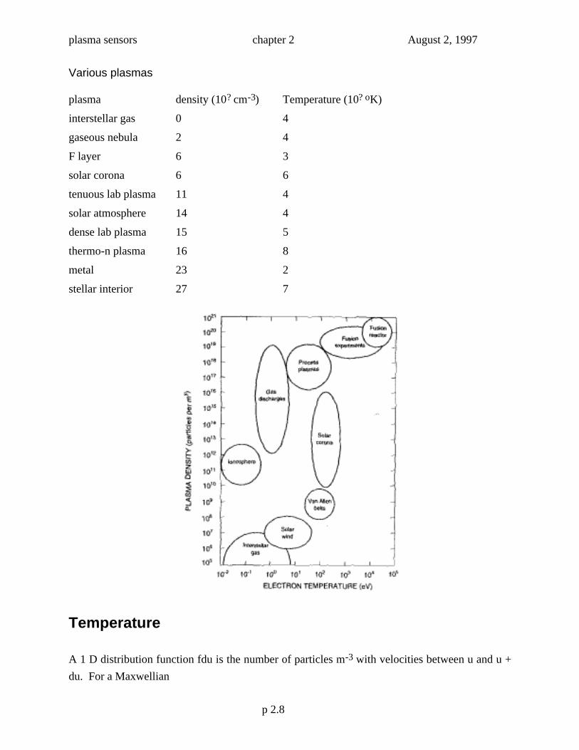
Various plasmas
plasma density (10? cm-3) Temperature (10? oK)
interstellar gas 0 4
gaseous nebula 2 4
F layer 6 3
solar corona 6 6
tenuous lab plasma 11 4
solar atmosphere 14 4
dense lab plasma 15 5
thermo-n plasma 16 8
metal 23 2
stellar interior 27 7
Temperature
A 1 D distribution function fdu is the number of particles m-3 with velocities between u and u +
du. For a Maxwellian
p 2.8
plasma sensors chapter 2 August 2, 1997
f u( ) = Ae − 1
2mu2 / kT( )
where k = 1.38x10⁻²³ J/0K. The density n is given by
n = f u( )−∞
∞
∫ du .
Then n = A e − 1
2mu 2 / kT( )
−∞
∞
∫ du implies A = nm
2πkT
1 / 2
.
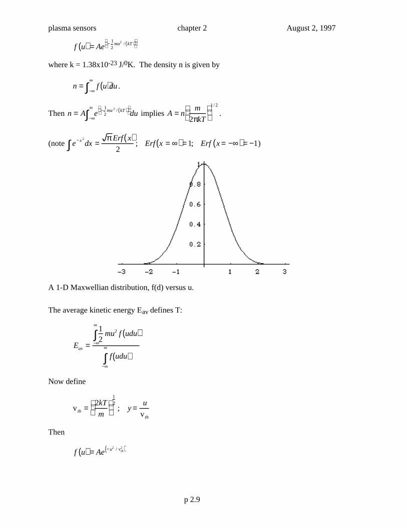
(note e− x 2
∫ dx =π Erf x( )
2; Erf x = ∞( ) = 1; Erf x = −∞( ) = −1)
A 1-D Maxwellian distribution, f(d) versus u.
The average kinetic energy Eav defines T:
Eav =
12
mu2 f udu( )−∞
∞
∫
f udu( )−∞
∞
∫
Now define
v th =2kT
m
1
2; y =
u
v th
Then
f u( ) = Ae − u2 / vth2( )
p 2.9
plasma sensors chapter 2 August 2, 1997
Eav =
12
Amv th3 e− y 2
y2dy−∞
∞
∫
Avth e−y 2
dy−∞
∞
∫=
− 12
e− y2
y
−∞
∞
− − 12
e− y 2
dy−∞
∞
∫
e− y 2
dy−∞
∞
∫=
mv th2
4=
kT
2
(Integrate by parts adb∫ = ab[ ] − bda∫ , with
a = y; db = ye −y 2
dy; da = dy; b = −e− y
2
2; )
Extension to a 3-D distribution follows:
f u, v,w( ) = A3e − 1
2m u2 +v 2 + w 2( ) / kT( )
A3 = nm
2πkT
3 / 2
Eav =A3
1
2m u2 + v2 + w2( )e −
1
2m u 2 +v 2 + w 2( ) / kT
dudvdw∫∫∫
A3e − 1
2m u2 + v 2 + w2( ) / kT
dudvdw∫∫∫
By symmetry, we can evaluate one term in the numerator and multiply by 3:
Eav =3
12
mu2e −1
2mu 2 / kT
du e −
1
2m v 2 + w 2( ) / kT
∫∫ dudvdw
−∞
∞
∫
e − 1
2mu2 / kT
du e − 1
2m v 2 + w 2( ) / kT
∫∫ dvdw
−∞
∞
∫=
3
2kT
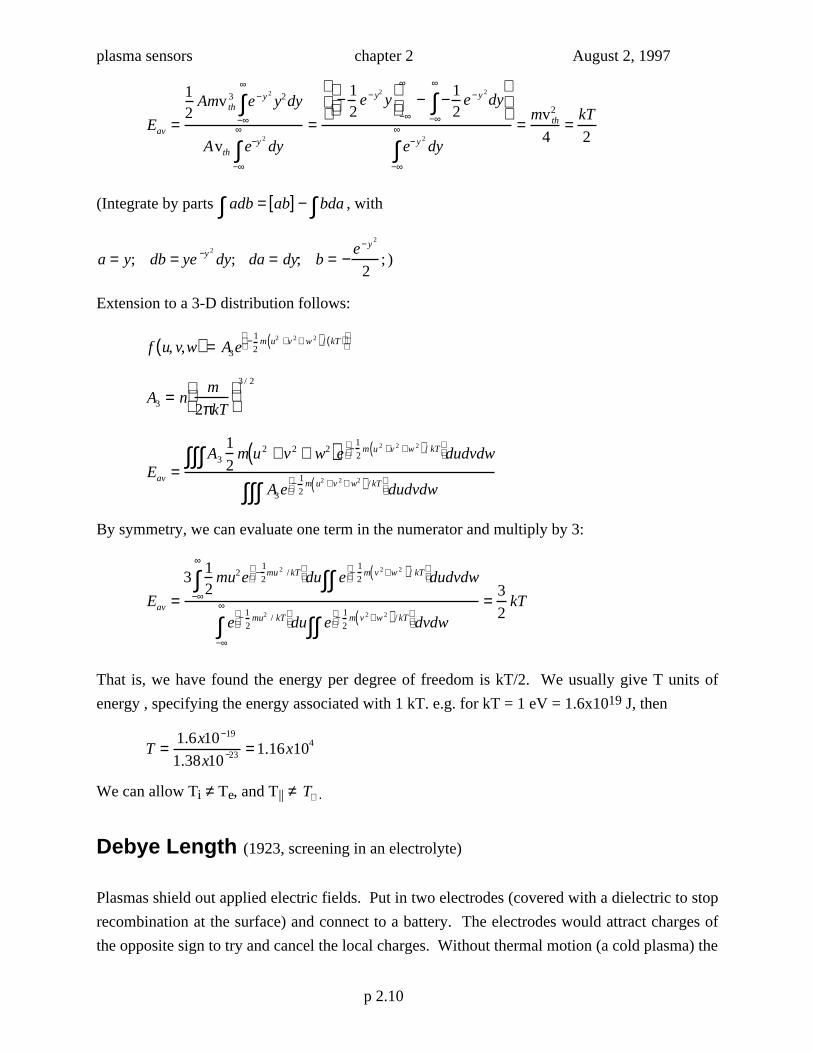
That is, we have found the energy per degree of freedom is kT/2. We usually give T units of
energy , specifying the energy associated with 1 kT. e.g. for kT = 1 eV = 1.6x10¹⁹ J, then
T =1.6x10⁻¹⁹
1.38x10−23 = 1.16x10⁴
We can allow Ti ≠ Te, and T|| ≠ T⊥ .
Debye Length (1923, screening in an electrolyte)
Plasmas shield out applied electric fields. Put in two electrodes (covered with a dielectric to stop
recombination at the surface) and connect to a battery. The electrodes would attract charges of
the opposite sign to try and cancel the local charges. Without thermal motion (a cold plasma) the
p 2.10
plasma sensors chapter 2 August 2, 1997
cancellation would be perfect. If the temperature is finite, the particles at the edge of the cloud
can escape. The edge occurs where the potential energy is approximately equal to kT. i.e. we can
expect to find potentials of order kT/e in plasmas.
Let f be the fractional departure of ne from ni over a spherical volume of radius r. Take
as an example a plasma with (very large) density n ≈ 1016 cm-3. Then the electrostatic field is
E =4πr3
3fne
1
r2 =4πrfne
3
i.e. if f = 10-6, then E = 6 kV/cm, and proportional to the radius of the charged space. This
electrostatic field operates to restore equilibrium, i.e. neutrality. Any departure from neutrality
tends to screen the original field; thermal agitation tends to disrupt neutrality, charged particle
density tends to maintain neutrality.
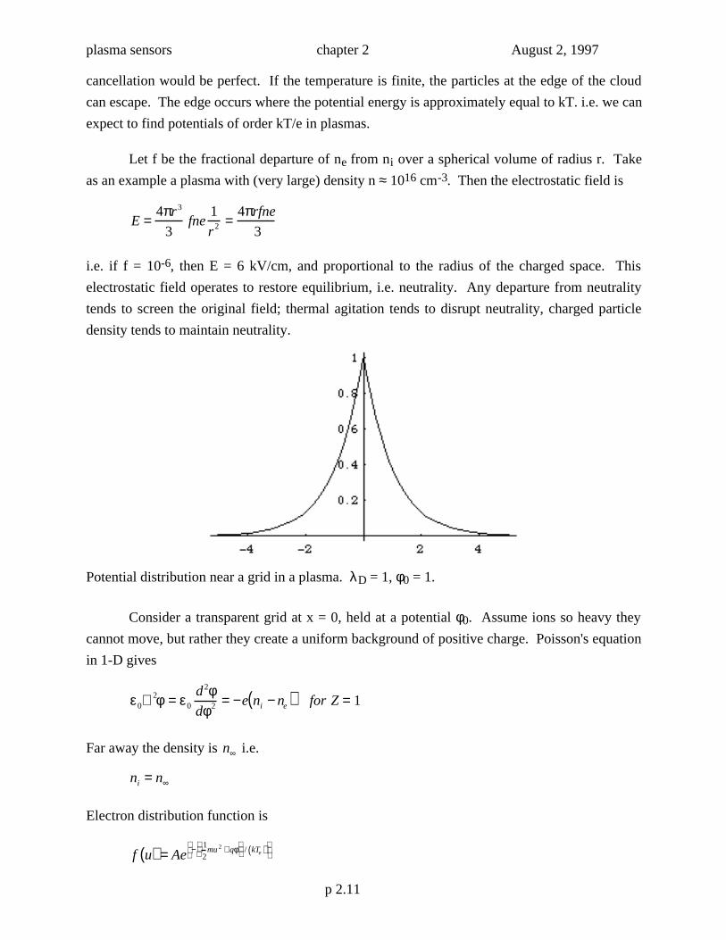
Potential distribution near a grid in a plasma. λD = 1, φ0 = 1.
Consider a transparent grid at x = 0, held at a potential φ0. Assume ions so heavy they
cannot move, but rather they create a uniform background of positive charge. Poisson's equation
in 1-D gives
ε0∇2φ = ε0
d2φdφ2 = −e ni − ne( ) for Z = 1
Far away the density is n∞ i.e.
ni = n∞
Electron distribution function is
f u( ) = Ae − 1
2mu 2 + qφ
/ kTe( )
p 2.11
plasma sensors chapter 2 August 2, 1997
(fewer particles where P.E. is high). Integrate over u, setting q = -e, with ne φ → 0( ) = n∞
ne = A e − 1
2mu2 − eφ
/ kTe( )
−∞
∞
∫ du = n∞e− eφ / kTe( )
Then Poisson's equation becomes, for small potentials,
ε0
d 2φdφ 2 = en∞ e−e φ / kTe( ) − 1( ) ≈ en∞
eφkTe
+1
2
eφkTe
2
+ ..
ε0
d 2φdφ 2 =
e2n∞
kTe
φ
i.e. φ = φ0e− x / λ D ; λD =
ε0kTe
ne2
1
2
λD = 7430kTe
n
1
2in m; kTe in eV
where n is used for n∞ .
Quasi neutral means that, for a system with size L >> λD, any concentrations of charge or
external potentials are shorted out. Outside the sheath ne ≈ ni to typically better than 1 part in
106. Plasma means L >> λD. Outside λD the effective potential is very small. For distances <<
λD the effective potential is equivalent to the bare Coulomb charge.
Plasma parameter: Debye shielding only valid if enough particles in cloud. Number of
particles in a Debye sphere is
ND = n4
3πλD
3
Let's do the above for a point charge q0 located at the origin, which produces a potential field
φ0 =q0
4πε0r
Consider an electron gas with density ne and temperature Te. Poisson's equation is
ε0∇2φ = −q0δ r( ) − e ni − ne( )
where δ(r) is the 3-D delta function. Note spherical cord system - we have
p 2.12
plasma sensors chapter 2 August 2, 1997
ε∇2 ≡ ε1
r2
∂∂r
r2 ∂φ∂r
As before, ne − ni = nieeφ / kTe( ) − ni ≈ nieφ / Te , and
ε0∇2φ = −q0δ r( ) +
ne2
kTe
φ
with a solution
φ(r) =q0
re− r / λD ; λD =
ε0kTe
ne2
1
2
If the ions can participate (quasi static conditions) then we can assume a M-B distribution for
both ions and electrons, and assuming ne = ni = n∞ = n at infinity,
ne = n∞e−e φ / kTe( ) ni = n∞e eφ / kTe( )
Poisson's equation becomes
ε0∇2φ = −q0δ r( ) − e ni − ne( ) = −q0δ r( ) − en eeφ / kTi( ) − e−eφ / kTe( )( )
≈ −q0δ r( ) + e2nφ 1kTi
+ 1kTe
In this case the Debye length is given by
λD =ε0k
ne2 1/ Te +1/ Ti( )
1
2
In the expansion of the Exp function we assumed that the potential energy eφ << the kinetic
energy. We return to this later.
Plasma Oscillations
Consider a dynamic situation. When electrons attempt to screen out a net positive charge they
will overshoot, because they have a mass and thus a momentum. The electrons can oscillate, with
the Coulomb force acting as the restoring force and the mass of the electron as the inertia.
p 2.13
plasma sensors chapter 2 August 2, 1997
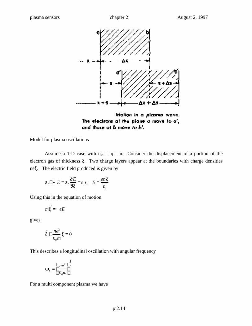
Model for plasma oscillations
Assume a 1-D case with ne = ni = n. Consider the displacement of a portion of the
electron gas of thickness ξ. Two charge layers appear at the boundaries with charge densities
neξ. The electric field produced is given by
ε0∇• E = ε0
∂E
∂ξ= en; E =
enξε0
Using this in the equation of motion
m˙ ̇ ξ = −eE
gives
˙ ̇ ξ +ne2
ε0mξ = 0
This describes a longitudinal oscillation with angular frequency
ωp =ne2
ε0m
1
2
For a multi component plasma we have
p 2.14
plasma sensors chapter 2 August 2, 1997
ωp =nσqσ
2
ε0mσ
12
∑
We can also consider other modes of oscillation because there are additional degrees of
freedom corresponding to relative motion between the different kind of particles. For an electron
- ion plasma with ni = ne the above equation corresponds to an out of phase oscillation between
electrons and ions, which may be viewed as an optical mode. The other branch may be viewed
as an acoustic mode.
Find radio waves will only propagate with frequencies > plasma frequency
But use lower frequencies so they reflect back to earth.
In metals we have contained ions and free electrons. i.e. should be able to observe oscillations.
According to quantum mechanics there should be energy levels separated by hωp/(2π). Pass
electrons through a foil, find electrons sometimes lose energy hωp/(2π) to foil.
Discreteness
λD and ωp are computed from 4 parameters, m, e,1/n and T. These are the basic quantities
characterizing a classical plasma; they are related to the discrete nature of the particles. They
describe the mass, charge, average volume and average kinetic energy per particle. Introduce a
theoretical limit in which the individuality of the particles is suppressed, and the plasma takes on
a medium like property. Cut each particle into finer and finer pieces, so that the discrete
parameters all approach 0. In doing this we keep certain fluid like parameters constant; the mass
density mn, the charge density ne, the kinetic energy density nT,.
Look for a dimensionless parameter which can be constructed from these 4 discrete
parameters. Write
mα 1/ n( )βT γ e[ ] =1
where we are considering only dimensions. e has dimensions M[ ]1 / 2L[ ]3 / 2
T −1[ ] , so that
α + γ +1/ 2 = 0; 3β + 2γ + 3/ 2 = 0; − 2γ −1 = 0
i.e. α = 0; β = −1/6; γ = −1/ 2
this is the only solution. That is, the discreteness parameter is any power of the function
en1 / 6T−1 / 2
p 2.15
plasma sensors chapter 2 August 2, 1997
taking the 3 rd power gives us the dimensionless parameter
g = en1 / 6T− 1/ 2( )3= 1/ nλD
3( ) ≈ 1/ ND
g is called the plasma parameter, which measures the ratio between potential and kinetic
energies. It is small, and used as an expansion parameter.
Collective versus individual behavior
Consider the equation of motion for a density fluctuation in an electron gas. Deal with point
particles and charges, so that the density field is given by the superposition of 3=D delta
functions
ρ r ( ) = δ r − r i( )i = 1
n∑
where ri is the position of the i-th electron. Consider a cube of unit volume with periodic
boundary conditions, so n is the number density. The spatial Fourier components of any
fluctuations is
ρk = ρ r ( )∫ e− ik • r dr = e− ik • r i
i∑
Differentiate twice with respect to time
˙ ̇ ρ k = − k • v i( )2+ ik • ˙ v i[ ]e−ik • r i
i∑
vi is the velocity of the it electron. The acceleration ˙ v i is calculated from the force acting on the
electron from all other electrons and the positive charge background
˙ v i = −1
m
∂∂r i
e2
r i − r jj ≠i∑
We want to write this in a different form, so note that
∇2 1
r − r '= −4πδ r − r '( )
i.e.∂∂r
1
r − r '= −4π δ r − r '( )∫
Now an identity is
p 2.16
plasma sensors chapter 2 August 2, 1997
δ r − r '( ) = eik • r −r '( )k
∑
so that
∂∂r i
1
r − r '= −4π e ik • r −r '( )∫
k∑ dr = 4πi
k
k2 e ik • r −r '( )k
∑
Therefore
˙ v i = −i4πe2
m
k
k2 eik • ri −rj( )k
∑j ≠i∑ = −i
4πe2
m
k
k2 ρkeik • ri
k∑
Substituting this into the expression for the acceleration gives
˙ ̇ ρ k = − k • v i( )2e− ik • r i −
4πe2
m
k • q
q2 ρk −q ρqq
∑
i∑
rewrite this by separating out the term with k = q on the HS to give
˙ ̇ ρ k + ω p2ρk =− k • v i( )2
e−ik • r i −4πe2
m
k •q
q2 ρk − qρqq≠ k∑
i∑
i.e. fluctuations occur at the plasma frequency as long as the RHS terms can be neglected.
Consider a Maxwellian distribution. Then the first term gives
k • v i( )2e− ik • r i[ ]
i∑ = e− ik •r i
i∑ k • v ( )2
f v( )∫ dv = k2 T
mρk
The second term involves the product of two density fluctuations. The density fluctuation for q
≠ 0 is the sum of exponential terms with randomly varying phases, his term can be ignored.
Then the condition for collective oscillation becomes
k <4πne2
T
1
2
=1
λD
For short wavelengths, however, the plasma behaves as a system of individual charges., and the
first term on the RHS determines what happens
p 2.17
plasma sensors chapter 2 August 2, 1997
Applications of Plasma Physics
Characterize by n, T, or better N. n from 106 to 1034, T from 0.1 to 106 eV. This is a large
range, e.g.. the density of a neutron star is 1015 times water.
Gas Discharges
Langmuir, Tonks. Originally researching vacuum tubes. Weakly ionized glows and positive
columns. T ≈ 2 eV, 1014 < n < 1018 m-3. Discovered shielding, (sheath as a dark layer ). Now
applicable as mercury rectifiers, thyratrons, ignitrons, spark gaps, welding arcs, neon lights,
lightning.
Controlled Thermonuclear Fusion1929: Atkinson and Houterman proposed that Fusion might explain the energy of stars. Beam
target interactions demonstrated reality, but Ein >> Eout (Rutherford: Fusion Energy is
‘Moonshine’).
early 1940’s: discussions of possible laboratory experiments.
late 1940’s: possible geometry discussed.
early 1950’s: H bomb.
1951: Peron claimed Richter solved problem.
< 1958: Classified programs by USA, USSR, UK (because copious neutrons might be used to
create fissile material for bombs).
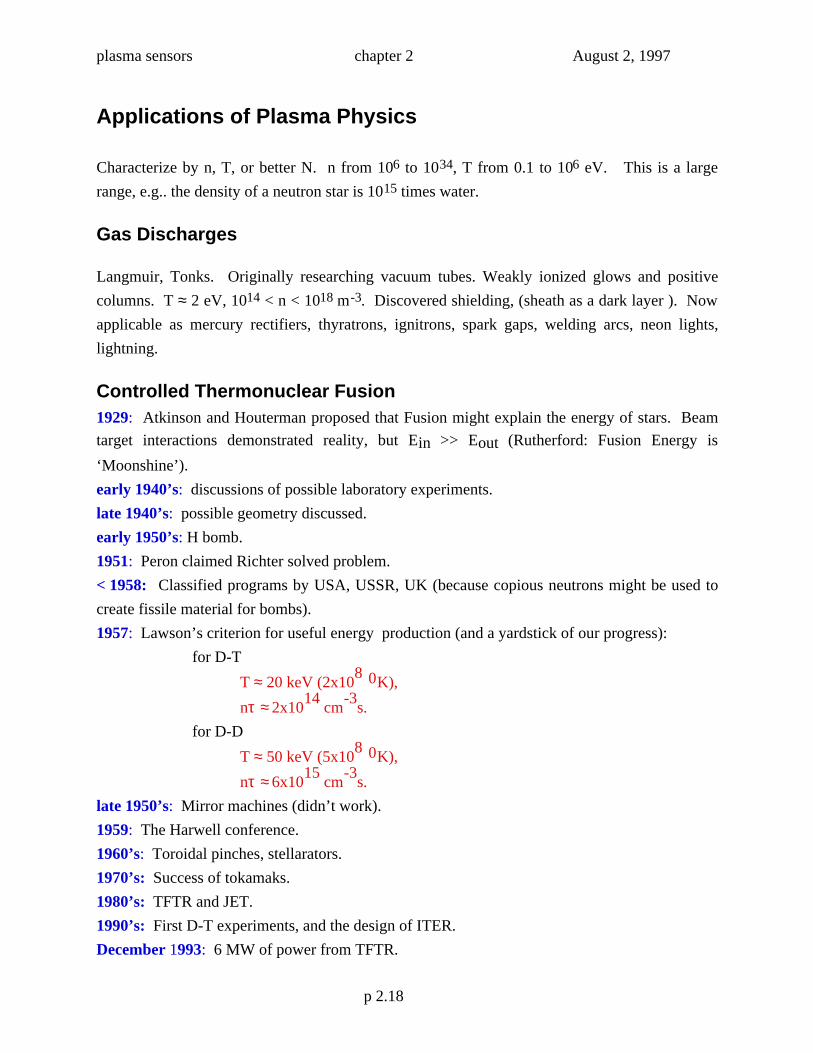
1957: Lawson’s criterion for useful energy production (and a yardstick of our progress):
for D-T
T ≈ 20 keV (2x10⁸ 0K),
nτ ≈ 2x10¹⁴
cm-3
s.
for D-D
T ≈ 50 keV (5x10⁸ 0K),
nτ ≈ 6x10¹⁵
cm-3
s.
late 1950’s: Mirror machines (didn’t work).
1959: The Harwell conference.
1960’s: Toroidal pinches, stellarators.
1970’s: Success of tokamaks.
1980’s: TFTR and JET.
1990’s: First D-T experiments, and the design of ITER.
December 1993: 6 MW of power from TFTR.
p 2.18
plasma sensors chapter 2 August 2, 1997
FROM THE DEBATE ON THE JET NUCLEAR FUSION PROJECT, THE HOUSE OF
LORDS, 1987
Earl Ferrers:
My Lords, what kind of thermometer reads a temperature of 140 million
degrees centigrade without melting?
Viscount Davidson:
My Lords, I should think a rather large one.
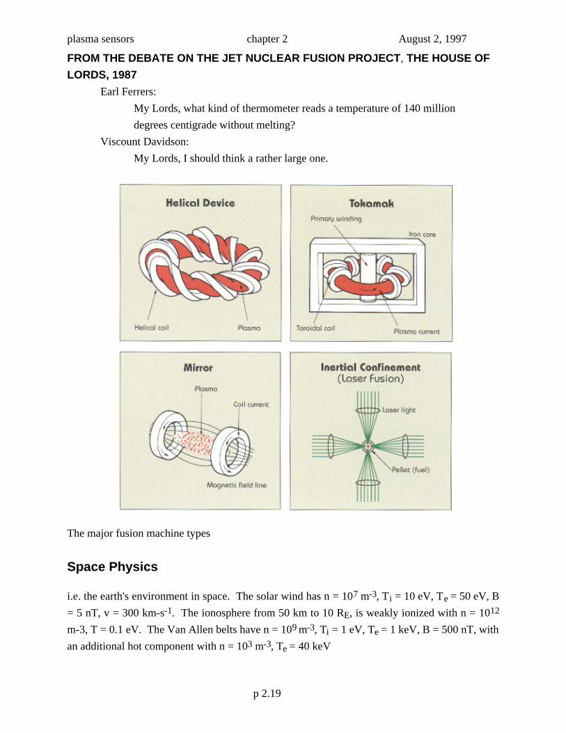
The major fusion machine types
Space Physics
i.e. the earth's environment in space. The solar wind has n = 107 m-3, Ti = 10 eV, Te = 50 eV, B
= 5 nT, v = 300 km-s-1. The ionosphere from 50 km to 10 RE, is weakly ionized with n = 1012
m-3, T = 0.1 eV. The Van Allen belts have n = 109 m-3, Ti = 1 eV, Te = 1 keV, B = 500 nT, with
an additional hot component with n = 103 m-3, Te = 40 keV
p 2.19
plasma sensors chapter 2 August 2, 1997
Astrophysics
For example stellar interiors and atmospheres, such as the sun with a core T = 2 keV and the
solar corona with T 200 eV. Interstellar medium of hydrogen with n = 106 m-3. Stars in
galaxies can be considered like particles in a plasma. Pulsars can be considered as plasmas.
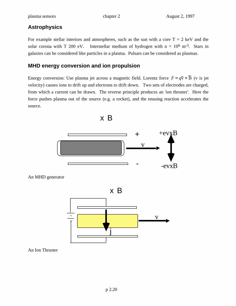
MHD energy conversion and ion propulsion
Energy conversion: Use plasma jet across a magnetic field. Lorentz force F = qv × B (v is jet
velocity) causes ions to drift up and electrons to drift down. Two sets of electrodes are charged,
from which a current can be drawn. The reverse principle produces an 'ion thruster'. Here the
force pushes plasma out of the source (e.g. a rocket), and the ensuing reaction accelerates the
source.
x B
+
-
v
+evxB
-evxB
An MHD generator
x B
+
-
v
j
An Ion Thruster
p 2.20
plasma sensors chapter 2 August 2, 1997
Solid state
Free electrons and holes constitute the same sort of oscillations and instabilities as in a gaseous
plasma. Lattice effects are equivalent to reducing the collision frequency from that expected in a
solid (n ≈ 1029 m-3). The holes have a very low effective mass.
Gas lasers
Use a gas discharge to pump, i.e. to invert the population of states.
The brain
p 2.21
plasma sensors chapter 2 August 2, 1997
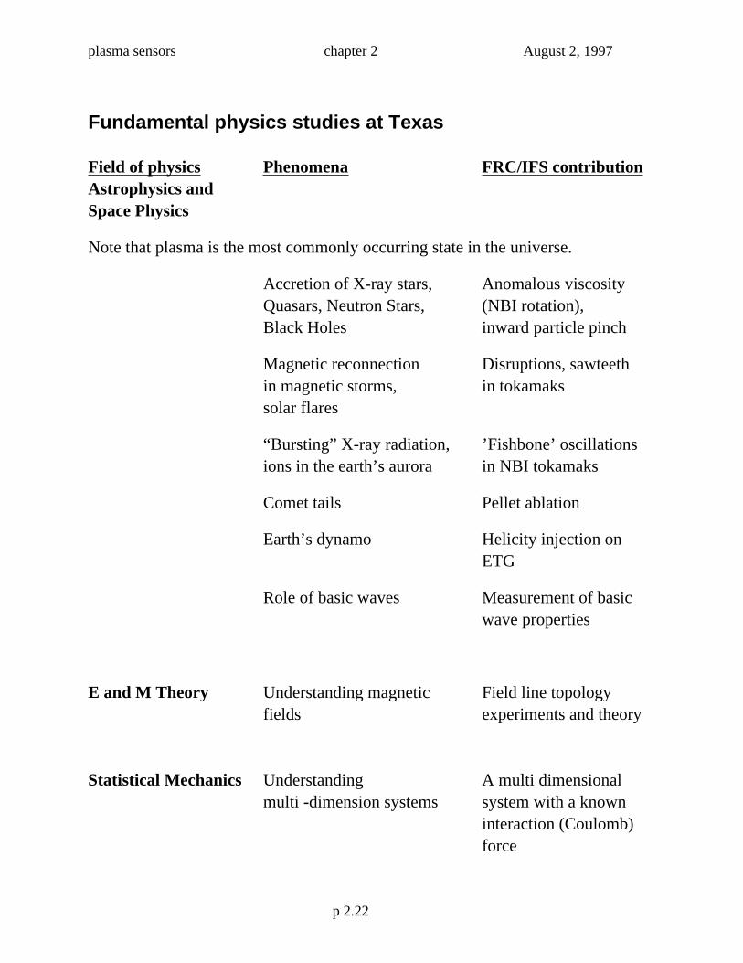
Fundamental physics studies at Texas
Field of physics Phenomena FRC/IFS contributionAstrophysics andSpace Physics
Note that plasma is the most commonly occurring state in the universe.
Accretion of X-ray stars, Anomalous viscosityQuasars, Neutron Stars, (NBI rotation),Black Holes inward particle pinch
Magnetic reconnection Disruptions, sawteethin magnetic storms, in tokamakssolar flares
“Bursting” X-ray radiation, ’Fishbone’ oscillations ions in the earth’s aurora in NBI tokamaks
Comet tails Pellet ablation
Earth’s dynamo Helicity injection on ETG
Role of basic waves Measurement of basic wave properties
E and M Theory Understanding magnetic Field line topologyfields experiments and theory
Statistical Mechanics Understanding A multi dimensional multi -dimension systems system with a known
interaction (Coulomb) force
p 2.22
plasma sensors chapter 2 August 2, 1997
Field of physics Phenomena FRC/IFS contribution
Turbulence andNon - linearDynamics
Note the excellent non perturbing plasma diagnostics available
Turbulent transport Turbulent transport
Understanding the Experimental control of phenomena due to drives and stabilizingnonlinearities terms, coherent structures,
breaking of time reversibility.
Required statistical analysis Developing statistical analysis techniques
Required renormalization Developing renormalization theories theories
Prediction capabilities Neural network forecasting of disruptions
All Aspectsof Physics
Required Hamiltonian Developing Hamiltonian mechanics mechanics
p 2.23
plasma sensors chapter 2 August 2, 1997
Applied physics and engineering studies at Texas
Field FRC/IFS contribution
Atomic Physics Line identification using the plasma as a source
Numerical Development of adaptive grid techniques
Tomography Development of analysis techniques
Control Engineering Fast real time digital feedback systems
Structural Engineering Development and use of high strength coppers
p 2.24
plasma sensors chapter 2 August 2, 1997
Research at the Fusion Research Center
Research opportunities at the FRC can be found at our home page
(http://w3fusion.ph.utexas.edu/frc/). Below are some details.
1. The linear machine
We are writing a proposal to NSF to try and obtain funding for this. We propose to build
an experiment to investigate the nonlinear regimes of kinetic instabilities. We will study the
transitions from the instability onset near its threshold to the coherent nonlinear states that
enhance plasma transport. We intend to verify if a recently developed theory of weakly unstable
kinetic modes in a driven system can explain different responses that can arise in the experiment.
This study is of interest as a precursor to the investigation of fully developed turbulence. We
will attempt to determine if an intrinsic kinetic description is needed to describe the observations
or whether an averaged fluid description is applicable in a collisionless plasma. For example, it
is now known that the collisionality, often assumed to be unimportant, is enhanced for the small
group of particles at the resonance and can effect the character of the response.
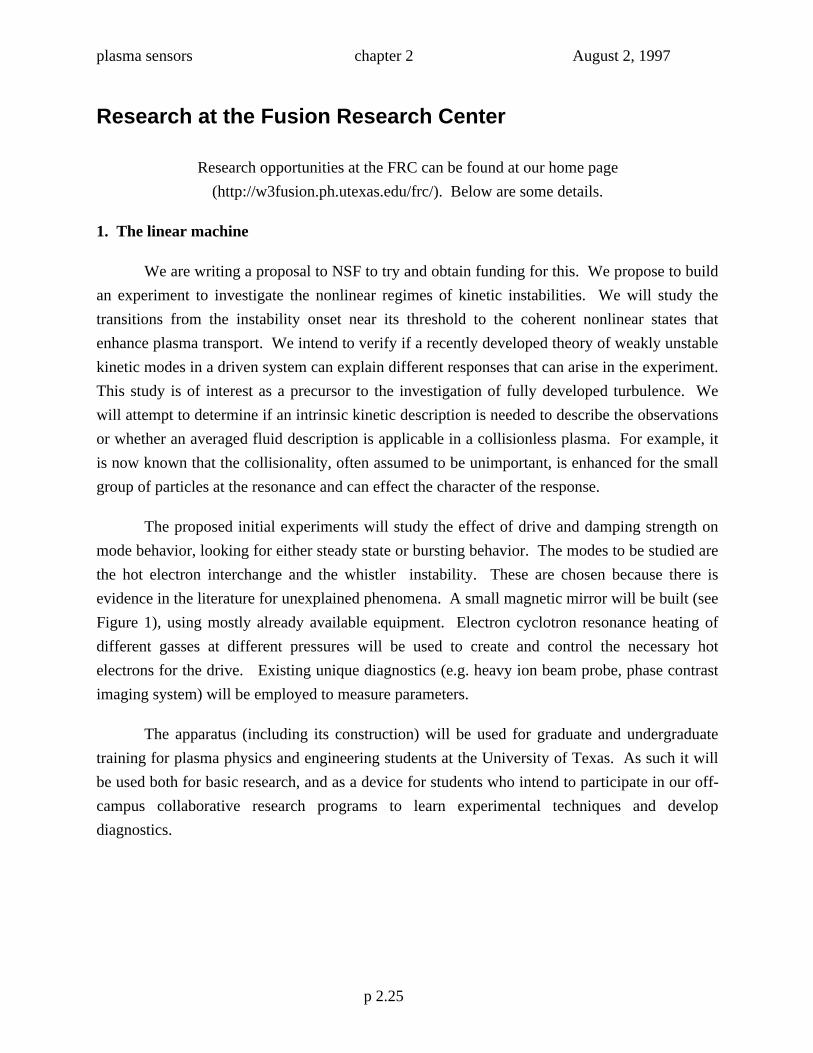
The proposed initial experiments will study the effect of drive and damping strength on
mode behavior, looking for either steady state or bursting behavior. The modes to be studied are
the hot electron interchange and the whistler instability. These are chosen because there is
evidence in the literature for unexplained phenomena. A small magnetic mirror will be built (see
Figure 1), using mostly already available equipment. Electron cyclotron resonance heating of
different gasses at different pressures will be used to create and control the necessary hot
electrons for the drive. Existing unique diagnostics (e.g. heavy ion beam probe, phase contrast
imaging system) will be employed to measure parameters.
The apparatus (including its construction) will be used for graduate and undergraduate
training for plasma physics and engineering students at the University of Texas. As such it will
be used both for basic research, and as a device for students who intend to participate in our off-
campus collaborative research programs to learn experimental techniques and develop
diagnostics.
p 2.25
plasma sensors chapter 2 August 2, 1997
vessel
fundamental second harmonic
Figure 1. The magnetic geometry and resonances of the mirror device. The broken linesrepresent magnetic flux lines. The solid lines are lines of constant magnetic field. Thefundamental and second harmonic resonances are shown.
2. Plasma Propulsion
We are working with NASA to obtain funding for students to work in Houston at the
Sonny Carter Center on a mirror machine. One of the most important issues being addressed
today in connection with human interplanetary travel is the crew's prolonged exposure to
weightlessness as well as the high radiation dosage which accrues during these long voyages.
From this point of view, it becomes crucial to achieve a minimum trip-time as well as to extend
the ship's acceleration schedule consistently with human and power plant limitations. However,
flexibility in these well-known "trajectory variables" remains limited by the capabilities of
conventional (constant specific impulse Isp) chemical engines. Trip-times remain "high" and
severely restricted by payload and fuel constraints while the acceleration time is negligibly short
compared to the total trip. The optimum rocket system would be one in which both thrust and
specific impulse are allowed to vary continuously depending on the conditions of flight.
p 2.26
plasma sensors chapter 2 August 2, 1997
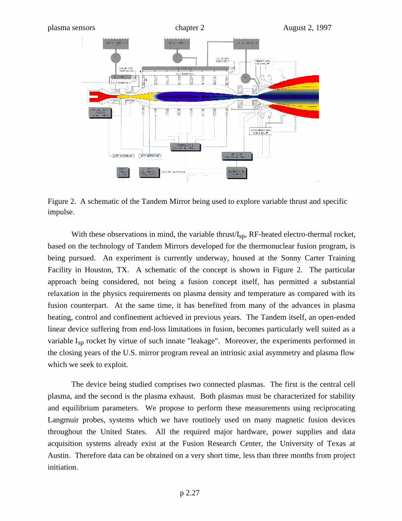
Figure 2. A schematic of the Tandem Mirror being used to explore variable thrust and specificimpulse.
With these observations in mind, the variable thrust/Isp, RF-heated electro-thermal rocket,
based on the technology of Tandem Mirrors developed for the thermonuclear fusion program, is
being pursued. An experiment is currently underway, housed at the Sonny Carter Training
Facility in Houston, TX. A schematic of the concept is shown in Figure 2. The particular
approach being considered, not being a fusion concept itself, has permitted a substantial
relaxation in the physics requirements on plasma density and temperature as compared with its
fusion counterpart. At the same time, it has benefited from many of the advances in plasma
heating, control and confinement achieved in previous years. The Tandem itself, an open-ended
linear device suffering from end-loss limitations in fusion, becomes particularly well suited as a
variable Isp rocket by virtue of such innate "leakage". Moreover, the experiments performed in
the closing years of the U.S. mirror program reveal an intrinsic axial asymmetry and plasma flow
which we seek to exploit.
The device being studied comprises two connected plasmas. The first is the central cell
plasma, and the second is the plasma exhaust. Both plasmas must be characterized for stability
and equilibrium parameters. We propose to perform these measurements using reciprocating
Langmuir probes, systems which we have routinely used on many magnetic fusion devices
throughout the United States. All the required major hardware, power supplies and data
acquisition systems already exist at the Fusion Research Center, the University of Texas at
Austin. Therefore data can be obtained on a very short time, less than three months from project
initiation.
p 2.27
plasma sensors chapter 2 August 2, 1997
3. EPEIUS
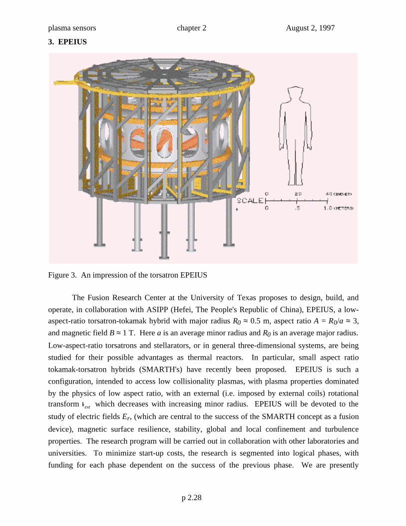
Figure 3. An impression of the torsatron EPEIUS
The Fusion Research Center at the University of Texas proposes to design, build, and
operate, in collaboration with ASIPP (Hefei, The People's Republic of China), EPEIUS, a low-
aspect-ratio torsatron-tokamak hybrid with major radius R0 ≈ 0.5 m, aspect ratio A = R0/a ≈ 3,
and magnetic field B ≈ 1 T. Here a is an average minor radius and R0 is an average major radius.
Low-aspect-ratio torsatrons and stellarators, or in general three-dimensional systems, are being
studied for their possible advantages as thermal reactors. In particular, small aspect ratio
tokamak-torsatron hybrids (SMARTH's) have recently been proposed. EPEIUS is such a
configuration, intended to access low collisionality plasmas, with plasma properties dominated
by the physics of low aspect ratio, with an external (i.e. imposed by external coils) rotationaltransform ι ext which decreases with increasing minor radius. EPEIUS will be devoted to the
study of electric fields Er, (which are central to the success of the SMARTH concept as a fusion
device), magnetic surface resilience, stability, global and local confinement and turbulence
properties. The research program will be carried out in collaboration with other laboratories and
universities. To minimize start-up costs, the research is segmented into logical phases, with
funding for each phase dependent on the success of the previous phase. We are presently
p 2.28
plasma sensors chapter 2 August 2, 1997
requesting funding only for Phase I, but a discussion of subsequent phases is included to indicate
our long term planning.
4. Alcator C-MOD
The FRC is presently involved in a collaboration with the MIT Plasma Science Fusion
Center (PSFC) in the study of turbulence and transport in tokamaks. An FRC staff member is
presently on site at MIT and we are hiring a post-doctoral fellow to assist, also on site. Most of
the other FRC staff are involved in the collaboration to varying degrees, either periodically
visiting the PSFC or participating in experiments and data analysis via remote access and video-
conferencing over the Internet.
We are adding turbulence diagnostics to the set of C-Mod profile diagnostics to attempt
to connect turbulence with transport The new diagnostic systems include
• a diagnostic neutral beam, which enables measurements of
- ion density fluctuations via beam-emission spectroscopy (BES),
- profiles of impurity density, temperature, and rotation velocities via charge-exchange
recombination spectroscopy (CXRS),
- toroidal current-density profile via the motional Stark effect (MSE).
• an electron-cyclotron-emission (ECE) heterodyne radiometer to measure profiles and
fluctuations of electron temperature,
• electrostatic probes for the measurement of fluctuating parameters in the edge plasma,
• an optical diagnostic to measure fluctuations in otherwise inaccessible regions of the edge
plasma.
In addition, we are assisting in the development of a phase-contrast imaging (PCI) system
for the study of ion-cyclotron waves and perhaps modifying the system for measurements of
plasma turbulence as well.
p 2.29
plasma sensors chapter 2 August 2, 1997
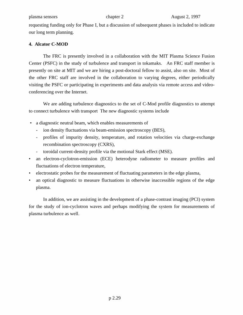
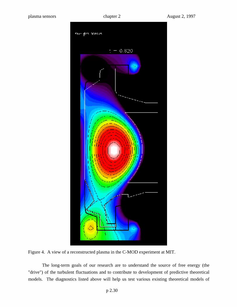
Figure 4. A view of a reconstructed plasma in the C-MOD experiment at MIT.
The long-term goals of our research are to understand the source of free energy (the
"drive") of the turbulent fluctuations and to contribute to development of predictive theoretical
models. The diagnostics listed above will help us test various existing theoretical models of
p 2.30
plasma sensors chapter 2 August 2, 1997
turbulent transport, most notably the IFS/PPPL model, which has recently been featured
prominently in the media (Dec. 6 issue of Science, subsequent articles in the N. Y. Times, etc.).
In the edge plasma, we wish to test the model that magnetic curvature serves as a drive of the
turbulence. Because C-Mod discharges are at especially high density and toroidal magnetic
field, turbulence measurements in C-Mod will also extend the empirical description of tokamak
turbulence to new plasma regimes.
5. DIII-D.
The FRC is also participating in turbulence and transport studies on the DIII-D tokamak
at General Atomics Co. in San Diego, CA. These involve i) collaborating with UCLA on ECE
fluctuation measurements and analysis, ii) collaborating with the University of Wisconsin,
Madison (UWM) on BES measurements and analysis, and iii) proposing and carrying out
experiments aimed at understanding the role of turbulence in tokamak transport. We also are
involved in high-resolution (both space and time) ECE measurements of electron temperature.
An FRC staff member, primarily involved in the ECE measurements, is on site at GA full time.
Like at C-Mod, other FRC staff either periodically visit GA during experiments, or participate
via remote access and video-conferencing.
Our physics program on DIII-D is similar to that on Alcator C-Mod, namely,
understanding the relevance of turbulence to transport by testing theoretical models of turbulent
transport. The FRC is therefore in a unique position of being involved in the same measurements
(BES and ECE) on the (soon-to-be) two remaining US tokamaks. Since the two machines are
considerably different (DIII-D is much larger, but of much lower density and toroidal field; DIII-
D employs uni-directional neutral beams for heating while C-Mod uses ion-cyclotron resonance
heating), these parallel measurements (and experiments) are not redundant, but allow us to
efficiently compare and contrast results in disparate plasmas, thereby gaining greater insights
into the fundamental mechanisms of the turbulence and transport.
p 2.31
plasma sensors chapter 2 August 2, 1997
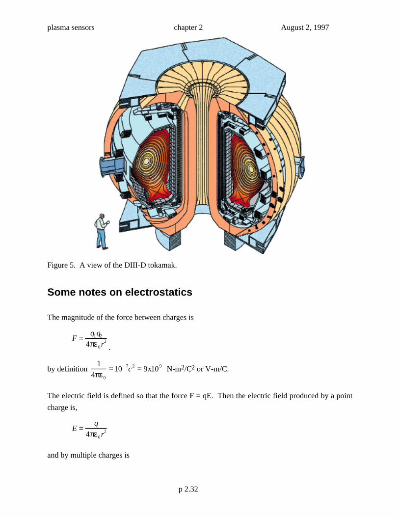
Figure 5. A view of the DIII-D tokamak.
Some notes on electrostatics
The magnitude of the force between charges is
F =q1q2
4πε0r2
.
by definition 1
4πε0
= 10− 7c2 = 9x10⁹ N-m2/C2 or V-m/C.
The electric field is defined so that the force F = qE. Then the electric field produced by a point
charge is,
E =q
4πε0r2
and by multiple charges is
p 2.32
plasma sensors chapter 2 August 2, 1997
E =qr i
4πε 0r3∑
where r i is the vector of magnitude ri.
The electrostatic potential at a point p is found from the work required to move the charge to a
point rp from infinity where the potential is 0. For a point charge the work dφ required to move
the charge a distance -E.dr, i.e.
φp = dφ0
φ p
∫ =−q
4πε0
dr
r2
r0
rp
∫ =q
4πε0
1
rp
−1
r0
=
q
4πε0rp
or, for multiple charges
φp =1
4πε0
qi
ri
∑
Gauss's theorem is
A • n dS = ∇ • A dVV∫
S∫
Poisson's equation: let the vector A = D = εE , so that
∇• εE dVV∫ = εE •n dS =
S∫ Q = ρdV
V∫
where ρ is charge density. Now let dV become vanishingly small
−∇ •εE =∇ • ε∇φ( ) = −ρ
Note the solution is
φ =1
4πε0
qdV
rV∫
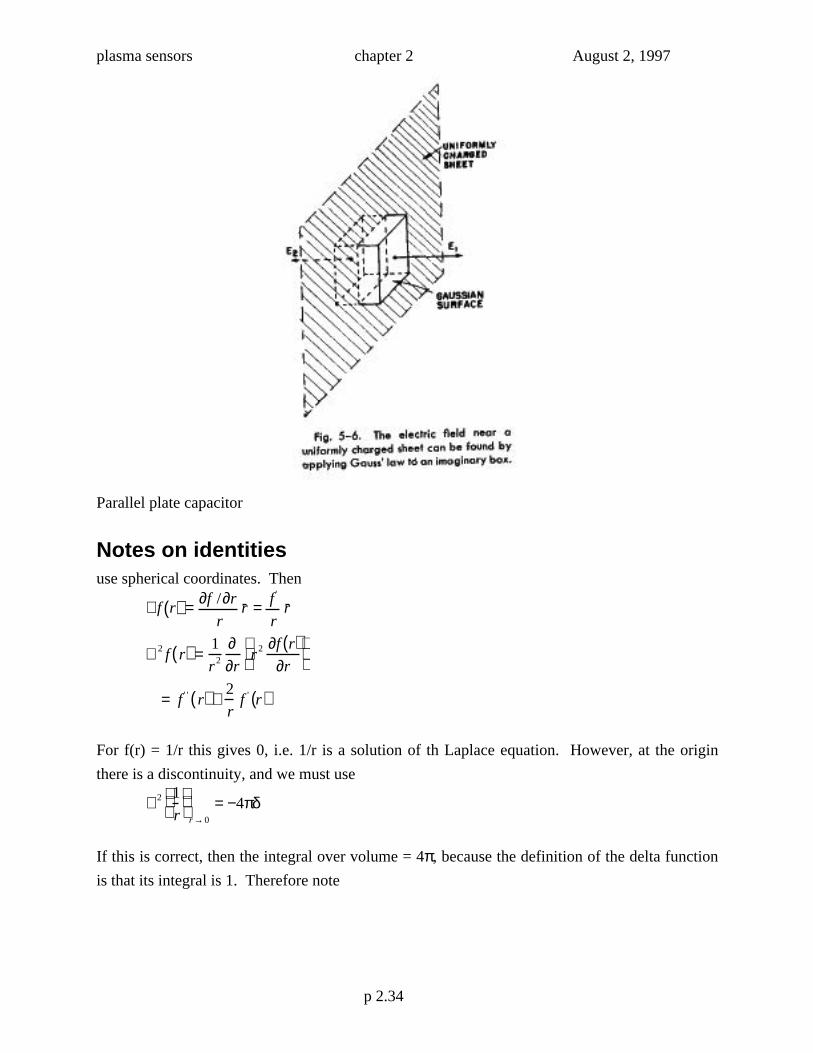
Application to a sheet charges, e.g. a parallel plate capacitor with each plate area A and charge q,
surface charge density s. See Feynman vol. 2?. Applying Gauss's flux theorem
εE • n dS =S∫ Q = ρdV
V∫
i.e. we have E = s/ε.
p 2.33
plasma sensors chapter 2 August 2, 1997
Parallel plate capacitor
Notes on identitiesuse spherical coordinates. Then
∇f r( ) = ∂f /∂r
rr = f '
rr
∇2 f r( ) =1
r2
∂∂r
r2 ∂f r( )∂r
= f ' ' r( ) +2
rf ' r( )
For f(r) = 1/r this gives 0, i.e. 1/r is a solution of th Laplace equation. However, at the origin
there is a discontinuity, and we must use
∇2 1
r
r → 0
= −4πδ
If this is correct, then the integral over volume = 4π, because the definition of the delta function
is that its integral is 1. Therefore note
p 2.34
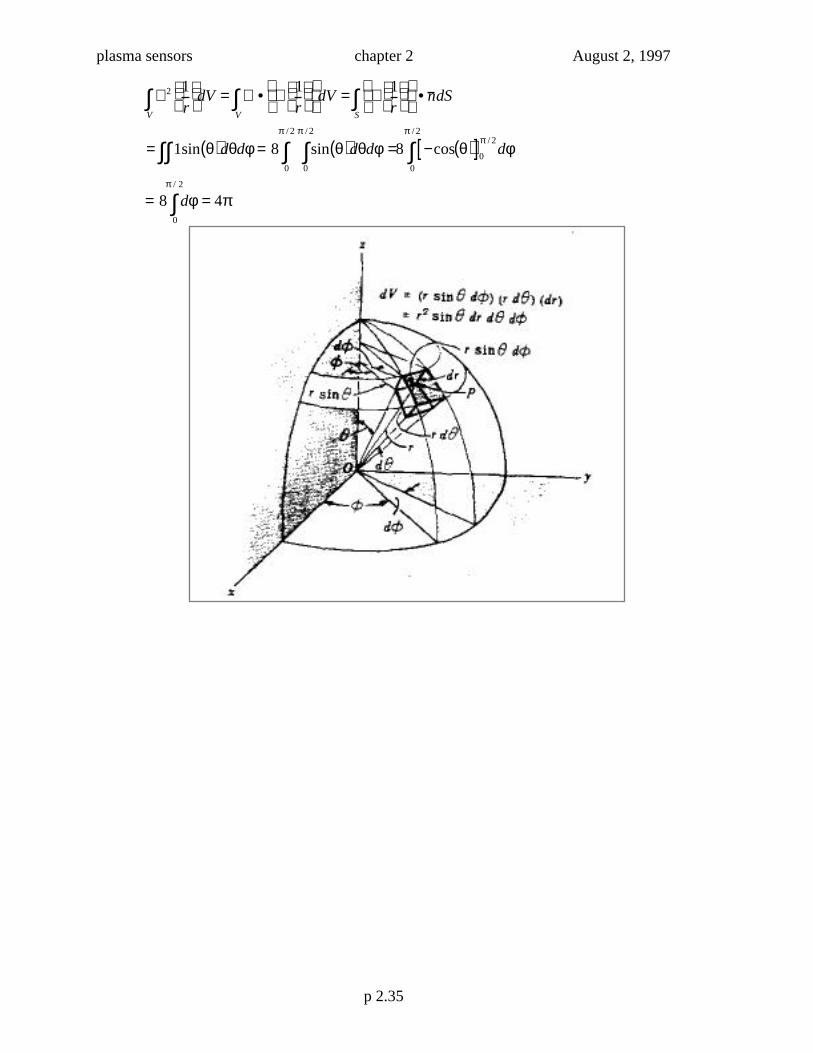
plasma sensors chapter 2 August 2, 1997
∇2 1r
V∫ dV = ∇ • ∇ 1
r
V∫ dV = ∇ 1
r
• n
S∫ dS
= 1sin θ( )dθdφ∫∫ = 8 sin θ( )dθdφ =0
π / 2
∫0
π / 2
∫ 8 −cos θ( )[ ]0
π / 2dφ
0
π / 2
∫
= 8 dφ0
π / 2
∫ = 4π
p 2.35
Recommended