
CERN Summer Student LecturePart 1, 19 July 2012
Introduction toMonte Carlo Techniquesin High Energy Physics
Torbjorn Sjostrand
How are complicated multiparticle events created?
How can such events be simulated with a computer?

Lectures Overview
today: Introduction the Standard ModelQuantum Mechanicsthe role of Event Generators
Monte Carlo random numbersintegrationsimulation
tomorrow: Physics hard interactionsparton showersmultiparton interactionshadronization
Generators Herwig, Pythia, SherpaMadGraph, AlpGen, . . .common standards
Torbjorn Sjostrand Introduction to Monte Carlo Techniques in High Energy Physics – lecture 1 slide 2/31
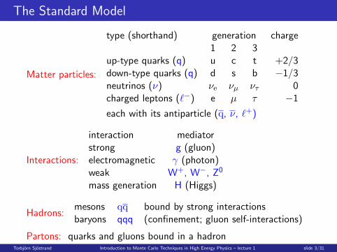
The Standard Model
Matter particles:
type (shorthand) generation charge1 2 3
up-type quarks (q) u c t +2/3down-type quarks (q) d s b −1/3neutrinos (ν) νe νµ ντ 0charged leptons (`−) e µ τ −1
each with its antiparticle (q, ν, `+)
Interactions:
interaction mediatorstrong g (gluon)electromagnetic γ (photon)weak W+, W−, Z0
mass generation H (Higgs)
Hadrons:mesons qq bound by strong interactionsbaryons qqq (confinement; gluon self-interactions)
Partons: quarks and gluons bound in a hadronTorbjorn Sjostrand Introduction to Monte Carlo Techniques in High Energy Physics – lecture 1 slide 3/31

Feynman Diagrams
incomingquarks
outgoingquarks
exchangedgluon
propagator
vertex
vertex
time
space
Introduce kinematics-dependent factors for incoming, outgoingand exchanged particles, and couplings for vertices:together they give the amplitude for the process.
Torbjorn Sjostrand Introduction to Monte Carlo Techniques in High Energy Physics – lecture 1 slide 4/31
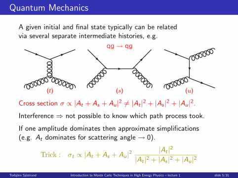
Quantum Mechanics
A given initial and final state typically can be relatedvia several separate intermediate histories, e.g.
qg! qg
(t) (s) (u)
Cross section σ ∝ |At + As + Au|2 6= |At |2 + |As |2 + |Au|2.
Interference ⇒ not possible to know which path process took.
If one amplitude dominates then approximate simplifications(e.g. At dominates for scattering angle → 0).
Trick : σt ∝ |At + As + Au|2|At |2
|At |2 + |As |2 + |Au|2
Torbjorn Sjostrand Introduction to Monte Carlo Techniques in High Energy Physics – lecture 1 slide 5/31

Fluctuations
n0 20 40 60 80 100 120 140 160 180
nP
-610
-510
-410
-310
-210
-110
1
10
210
310 CMS DataPYTHIA D6TPYTHIA 8PHOJET
)47 TeV (x10
)22.36 TeV (x10
0.9 TeV (x1)
| < 2.4η| > 0
Tp
(a)CMS NSD
Wide distribution ofthe number ofcharged particlesin an event,each particlewith continuum ofpossible momenta.
Combination ofQM processesat play.
So an infinityof final states,with a probabilisticspread of properties.
Torbjorn Sjostrand Introduction to Monte Carlo Techniques in High Energy Physics – lecture 1 slide 6/31

Complexity
Impossible to predict complete distribution of events from theory:
Strong interactions not solved (e.g. bound hadron states).
Even if, then production of ∼ 100 particlescomputationally impossible to handle.
Some simple tasks still ∼ solvable, e.g. qq → Z0 → `+`−.
But a quark/gluonshows up as a jet= a spray of hadrons.
Ill-defined borders+ underlying activity⇒ difficult interpretation.
Torbjorn Sjostrand Introduction to Monte Carlo Techniques in High Energy Physics – lecture 1 slide 7/31
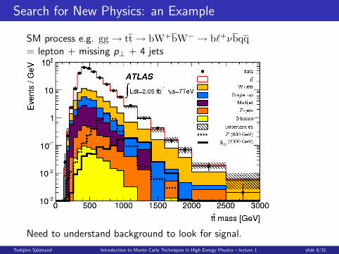
Search for New Physics: an Example
SM process e.g. gg → tt → bW+bW− → b`+νbqq= lepton + missing p⊥ + 4 jets
Need to understand background to look for signal.
Torbjorn Sjostrand Introduction to Monte Carlo Techniques in High Energy Physics – lecture 1 slide 8/31

Event Generator Philosophy
Divide et impera (Divide and conquer/rule; Latin proverb)
Way forward:
Accept approximate framework.
Evolution in “time”: one step at a time.
Each step “simple”, e.g. n-particle → (n + 1)-particle.
Diffferent mechanisms at different “time” epochs.
Computer algorithms for physics and bookkeeping.
Generate samples of events, just like experimentalists do.
Strive to predict/reproduce average behaviour & fluctuations.
Random numbers represent quantum mechanical choices.
Torbjorn Sjostrand Introduction to Monte Carlo Techniques in High Energy Physics – lecture 1 slide 9/31

Welcome to Monte Carlo!
Torbjorn Sjostrand Introduction to Monte Carlo Techniques in High Energy Physics – lecture 1 slide 10/31
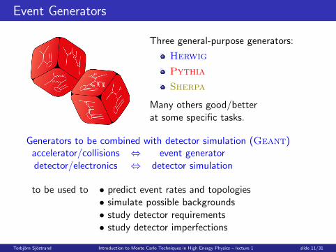
Event Generators
Three general-purpose generators:
Herwig
Pythia
Sherpa
Many others good/betterat some specific tasks.
Generators to be combined with detector simulation (Geant)accelerator/collisions ⇔ event generatordetector/electronics ⇔ detector simulation
to be used to • predict event rates and topologies• simulate possible backgrounds• study detector requirements• study detector imperfections
Torbjorn Sjostrand Introduction to Monte Carlo Techniques in High Energy Physics – lecture 1 slide 11/31

The Main Physics Components (in Pythia)
More tomorrow!
Torbjorn Sjostrand Introduction to Monte Carlo Techniques in High Energy Physics – lecture 1 slide 12/31

How to Compose a Complete Dinner
1 pick main course (≈ hard process = ME ⊕ PDF)
2 pick matching first course (≈ ISR)
3 pick matching dessert (≈ FSR)
4 pick side dishes and drinks (≈ MPI)
5 pick coffee/tea & cookies (≈ hadronization)
6 pick after-dinner snacks (≈ decays)
7 pick plates, cutlery, table setting (≈ administrative structure)
thousands of possible (published) recipes
uncountable combinations
never identical results (meat, spices, temperature, . . . )
Having a Higgs event ≈ having beef for dinner.(Don’t look down on the work of the chef!)
Torbjorn Sjostrand Introduction to Monte Carlo Techniques in High Energy Physics – lecture 1 slide 13/31
Monte Carlo Methods
Torbjorn Sjostrand Introduction to Monte Carlo Techniques in High Energy Physics – lecture 1 slide 14/31

Random Numbers
Truly random R :• uniform distribution 0 < R < 1• no correlations in sequence
Example: radioactive decayEvent generation + detector simulation voracious users⇒ need pseudorandom computer algorithms
Deterministic:in simplest form Ri = f (Ri−1)more sophisticated Ri = f (Ri−1,Ri−2, . . . ,Ri−k)
Examples:
name k periodoldtimers 1 ∼ 109
L’Ecuyer 3 ∼ 1026
Marsaglia-Zaman 97 ∼ 10171
Mersenne twister 623 ∼ 10600
Torbjorn Sjostrand Introduction to Monte Carlo Techniques in High Energy Physics – lecture 1 slide 15/31

The Marsaglia Effect
2D-array: white if R < 0.5, black if R > 0.5:
Marsaglia: recursion ⇒ multiplets (Rmi ,Rmi+1, . . . ,Rmi+m−1),i = 1, 2, . . ., fall on parallel planes in m-dimensional hypercube.A small m spells disaster. Don’t play on your own!
Torbjorn Sjostrand Introduction to Monte Carlo Techniques in High Energy Physics – lecture 1 slide 16/31

Spatial vs. Temporal Problems
“Spatial” problems: no memory
1 What is the land area of your home country?
2 What is the integrated cross section of a process?
“Temporal” problems: has memory
1 Traffic flow: What is probability for a car to pass a givenpoint at time t, given traffic flow at earlier times?(Lumping from red lights, antilumping from finite size of cars!)
2 Radioactive decay: what is the probability for a radioactivenucleus to decay at time t, gven that it was created at time 0?
In reality normally combined into multidimensional problems
1 What is traffic flow in a whole city?
2 What is the probability for a radioactive nucleusto decay sequentially at several different times,each time into one of several possible channels?
Torbjorn Sjostrand Introduction to Monte Carlo Techniques in High Energy Physics – lecture 1 slide 17/31

Spatial methods
In practical applications often need not only value of integral,but also sample of randomly distributed points inside “area”:
represents quantum mechanical spread, like real data;
allows separation of messy multidimensional problems.
pq pq
!!/Z0
M2!!/Z0 = (pq + pq)
2
p"q p"
q
p"
f
p"
f
"
Example: qq → γ∗/Z 0 → ff is 2 → 2 but can be split into steps,that consecutively provide more information on the event:
1 production qq → γ∗/Z 0, notably choice of mass Mγ∗/Z0 ;2 choice of final flavour f = d,u, s, c,b, t, e−, νe, µ
−, νµ, τ−, ντ ;3 decay γ∗/Z 0 → ff, notably choice of rest frame polar angle θ;4 further steps, up to and including detector cuts.
Torbjorn Sjostrand Introduction to Monte Carlo Techniques in High Energy Physics – lecture 1 slide 18/31

Simple Integration
(flat Earthapproximation)
1 Pick x coordinate at random between horizontal limits.
2 Pick y coordinate at random between vertical limits.
3 Find whether point is inside Swiss border.
4 Repeat many times and keep statistics.
Area = width× height× #inside#tries
Torbjorn Sjostrand Introduction to Monte Carlo Techniques in High Energy Physics – lecture 1 slide 19/31

Integration of a function
Assume function f (x),x = (x1, x2, . . . , xn), n ≥ 1,where xi ,min < xi < xi ,max,and 0 ≤ f (x) ≤ fmax.
Then
Theorem
An n-dimensional integration ≡ an n + 1-dimensional volume∫f (x1, . . . , xn) dx1 . . .dxn ≡
∫ ∫ f (x1,...,xn)
01 dx1 . . .dxn dxn+1
So Monte Carlo integration of a functionis a simple generalization of area calculation.
Torbjorn Sjostrand Introduction to Monte Carlo Techniques in High Energy Physics – lecture 1 slide 20/31

Hit-and-miss Monte Carlo
If f (x) ≤ fmax in xmin < x < xmax
use interpretation as an area1 select
x = xmin + R (xmax − xmin)
2 select y = R fmax (new R!)
3 while y > f (x) cycle to 1
Integral as by-product:
I =
∫ xmax
xmin
f (x) dx = fmax (xmax − xmin)Nacc
Ntry= Atot
Nacc
Ntry
Binomial distribution with p = Nacc/Ntry and q = Nfail/Ntry,so error
δI
I=
Atot
√p q/Ntry
Atot p=
√q
p Ntry=
√q
Nacc−→ 1√
Naccfor p � 1
Torbjorn Sjostrand Introduction to Monte Carlo Techniques in High Energy Physics – lecture 1 slide 21/31

Analytical Solution
Same probability per unit area⇒ area to right of selected xis uniformly distributed fractionof whole area:∫ x
xmin
f (x ′) dx ′ = R
∫ xmax
xmin
f (x ′) dx ′
If know primitive function F (x) and know inverse F−1(y) then
F (x)− F (xmin) = R (F (xmax)− F (xmin)) = R Atot
=⇒ x = F−1(F (xmin) + R Atot)
Example:f (x) = 2x , 0 < x < 1, =⇒ F (x) = x2
F (x)− F (0) = R (F (1)− F (0)) =⇒ x2 = R =⇒ x =√
R
Torbjorn Sjostrand Introduction to Monte Carlo Techniques in High Energy Physics – lecture 1 slide 22/31
Importance Sampling
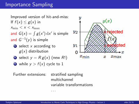
Improved version of hit-and-miss:If f (x) ≤ g(x) inxmin < x < xmax
and G (x) =∫
g(x ′) dx ′ is simple
and G−1(y) is simple
1 select x according tog(x) distribution
2 select y = R g(x) (new R!)
3 while y > f (x) cycle to 1
Further extensions: stratified samplingmultichannelvariable transformations. . .
Torbjorn Sjostrand Introduction to Monte Carlo Techniques in High Energy Physics – lecture 1 slide 23/31
Multidimensional Integrals
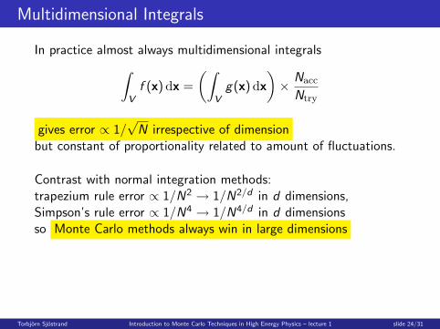
In practice almost always multidimensional integrals∫V
f (x) dx =
(∫V
g(x) dx
)× Nacc
Ntry
gives error ∝ 1/√
N irrespective of dimensionbut constant of proportionality related to amount of fluctuations.
Contrast with normal integration methods:trapezium rule error ∝ 1/N2 → 1/N2/d in d dimensions,Simpson’s rule error ∝ 1/N4 → 1/N4/d in d dimensionsso Monte Carlo methods always win in large dimensions
Torbjorn Sjostrand Introduction to Monte Carlo Techniques in High Energy Physics – lecture 1 slide 24/31
Temporal Methods: Radioactive Decays – 1
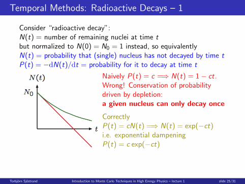
Consider “radioactive decay”:N(t) = number of remaining nuclei at time tbut normalized to N(0) = N0 = 1 instead, so equivalentlyN(t) = probability that (single) nucleus has not decayed by time tP(t) = −dN(t)/dt = probability for it to decay at time t
Naively P(t) = c =⇒ N(t) = 1− ct.Wrong! Conservation of probabilitydriven by depletion:a given nucleus can only decay once
CorrectlyP(t) = cN(t) =⇒ N(t) = exp(−ct)i.e. exponential dampeningP(t) = c exp(−ct)
Torbjorn Sjostrand Introduction to Monte Carlo Techniques in High Energy Physics – lecture 1 slide 25/31
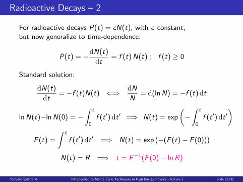
Radioactive Decays – 2
For radioactive decays P(t) = cN(t), with c constant,but now generalize to time-dependence:
P(t) = −dN(t)
dt= f (t) N(t) ; f (t) ≥ 0
Standard solution:
dN(t)
dt= −f (t)N(t) ⇐⇒ dN
N= d(lnN) = −f (t) dt
lnN(t)−lnN(0) = −∫ t
0f (t ′) dt ′ =⇒ N(t) = exp
(−
∫ t
0f (t ′) dt ′
)F (t) =
∫ t
f (t ′) dt ′ =⇒ N(t) = exp (−(F (t)− F (0)))
N(t) = R =⇒ t = F−1(F (0)− lnR)
Torbjorn Sjostrand Introduction to Monte Carlo Techniques in High Energy Physics – lecture 1 slide 26/31

The Veto Algorithm
What now if f (t) has no simple F (t) or F−1,but f (t) ≤ g(t), with g “nice”?
The veto algorithm
1 start with i = 0 and t0 = 0
2 + + i (i.e. increase i by one)
3 ti = G−1(G (ti−1)− lnR), i.e ti > ti−1
4 y = R g(t)
5 while y > f (t) cycle to 2
That is, when you fail, you keep on going from the time when youfailed, and do not restart at time t = 0. (Memory!)
Torbjorn Sjostrand Introduction to Monte Carlo Techniques in High Energy Physics – lecture 1 slide 27/31

The Veto Algorithm: Proof
define Sg (ta, tb) = exp(−
∫ tbta
g(t ′) dt ′)
P0(t) = P(t = t1) = g(t) Sg (0, t)f (t)
g(t)= f (t) Sg (0, t)
P1(t) = P(t = t2) =
∫ t
0dt1 g(t1)Sg (0, t1)
(1− f (t1)
g(t1)
)g(t) Sg (t1, t)
f (t)
g(t)
= f (t) Sg (0, t)
∫ t
0dt1 (g(t1)− f (t1)) = P0(t) Ig−f
P2(t) = · · · = P0(t)
∫ t
0dt1 (g(t1)− f (t1))
∫ t
t1
dt2 (g(t2)− f (t2))
= P0(t)
∫ t
0dt1 (g(t1)− f (t1))
∫ t
0dt2 (g(t2)− f (t2)) θ(t2 − t1)
= P0(t)1
2
(∫ t
0dt1 (g(t1)− f (t1))
)2
= P0(t)1
2I 2g−f
P(t) =∞∑i=0
Pi (t) = P0(t)∞∑i=0
I ig−f
i != P0(t) exp(Ig−f )
= f (t) exp
(−
∫ t
0g(t ′) dt ′
)exp
(∫ t
0dt1 (g(t1)− f (t1))
)= f (t) exp
(−
∫ t
0f (t ′) dt ′
)Torbjorn Sjostrand Introduction to Monte Carlo Techniques in High Energy Physics – lecture 1 slide 28/31
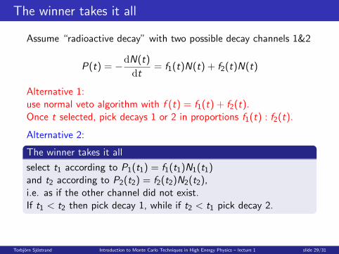
The winner takes it all
Assume “radioactive decay” with two possible decay channels 1&2
P(t) = −dN(t)
dt= f1(t)N(t) + f2(t)N(t)
Alternative 1:use normal veto algorithm with f (t) = f1(t) + f2(t).Once t selected, pick decays 1 or 2 in proportions f1(t) : f2(t).
Alternative 2:
The winner takes it all
select t1 according to P1(t1) = f1(t1)N1(t1)and t2 according to P2(t2) = f2(t2)N2(t2),i.e. as if the other channel did not exist.If t1 < t2 then pick decay 1, while if t2 < t1 pick decay 2.
Torbjorn Sjostrand Introduction to Monte Carlo Techniques in High Energy Physics – lecture 1 slide 29/31

The winner takes it all: proof
P1(t) = (f1(t) + f2(t)) exp
(−
∫ t
0(f1(t
′) + f2(t′))dt ′
)f1(t)
f1(t) + f2(t)
= f1(t) exp
(−
∫ t
0(f1(t
′) + f2(t′))dt ′
)= f1(t) exp
(−
∫ t
0f1(t
′) dt ′)
exp
(−
∫ t
0f2(t
′) dt ′)
Algorithm especially convenient when temporal and/or spatialdependence of f1 and f2 are rather different.
Torbjorn Sjostrand Introduction to Monte Carlo Techniques in High Energy Physics – lecture 1 slide 30/31

Summary
Nature is Quantum Mechanical.
LHC events contain infinite variability.
Use random numbers to pick among possible outcomes,
to give complete computer-generated LHC events,
hopefully predicting/reproducing average and spreadof any observable quantity.
Tomorrow:
A closer look at some of the key physics componentsof generators.
A survey of existing generators.
Torbjorn Sjostrand Introduction to Monte Carlo Techniques in High Energy Physics – lecture 1 slide 31/31
Recommended


