Introduction to Linear Regression
Arnaud Legrand
MOSIG Lecture
1 / 44
Outline
1 Simple Linear RegressionGeneral IntroductionFitting a Line to a Set of Points
2 Linear ModelLinear RegressionUnderlying HypothesisChecking hypothesisDecomposing the VarianceMaking PredictionsCon�dence interval
3 Conclusion
2 / 44
Outline
1 Simple Linear RegressionGeneral IntroductionFitting a Line to a Set of Points
2 Linear ModelLinear RegressionUnderlying HypothesisChecking hypothesisDecomposing the VarianceMaking PredictionsCon�dence interval
3 Conclusion
3 / 44
Outline
1 Simple Linear RegressionGeneral IntroductionFitting a Line to a Set of Points
2 Linear ModelLinear RegressionUnderlying HypothesisChecking hypothesisDecomposing the VarianceMaking PredictionsCon�dence interval
3 Conclusion
4 / 44
What is a regression?
Regression analysis is the most widely used statistical tool for understandingrelationships among variables. Several possible objectives including:
1 Prediction of future observations. This includes extrapolation since weall like connecting points by lines when we expect things to becontinuous
2 Assessment of the e�ect of, or relationship between, explanatoryvariables on the response
3 A general description of data structure (generally expressed in theform of an equation or a model connecting the response or dependentvariable and one or more explanatory or predictor variable)
4 De�ning what you should "expect" as it allows you to de�ne anddetect what does not behave as expected
The linear relationship is the most commonly found one
we will illustrate how it works
it is very general and is the basis of many more advanced tools(polynomial regression, ANOVA, . . . )
5 / 44
Outline
1 Simple Linear RegressionGeneral IntroductionFitting a Line to a Set of Points
2 Linear ModelLinear RegressionUnderlying HypothesisChecking hypothesisDecomposing the VarianceMaking PredictionsCon�dence interval
3 Conclusion
6 / 44
Starting With a Simple Data Set
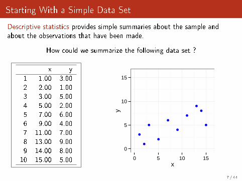
Descriptive statistics provides simple summaries about the sample andabout the observations that have been made.
How could we summarize the following data set ?
x y
1 1.00 3.002 2.00 1.003 3.00 5.004 5.00 2.005 7.00 6.006 9.00 4.007 11.00 7.008 13.00 9.009 14.00 8.0010 15.00 5.00
●
●
●
●
●
●
●
●
●
●
0
5
10
15
0 5 10 15x
y
7 / 44
Eyeball Method
●
●
●
●
●
●
●
●
●
●
0
5
10
15
0 5 10 15x
y
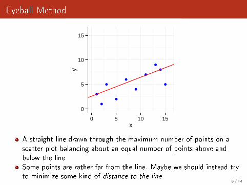
A straight line drawn through the maximum number of points on ascatter plot balancing about an equal number of points above andbelow the lineSome points are rather far from the line. Maybe we should instead tryto minimize some kind of distance to the line
8 / 44
Least Squares Line (1): What to minimize?
●
●
●
●
●
●
●
●
●
●
0
5
10
15
0 5 10 15x
y
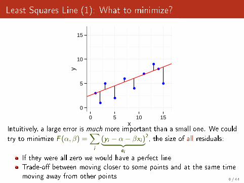
Intuitively, a large error is much more important than a small one. We could
try to minimize F (α, β) =∑i
(yi − α− βxi )︸ ︷︷ ︸ei
2, the size of all residuals:
If they were all zero we would have a perfect lineTrade-o� between moving closer to some points and at the same timemoving away from other points
9 / 44
Least Squares Line (2): Simple Formula
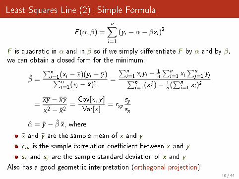
F (α, β) =n∑
i=1
(yi − α− βxi )2
F is quadratic in α and in β so if we simply di�erentiate F by α and by β,we can obtain a closed form for the minimum:
β =
∑ni=1(xi − x)(yi − y)∑n
i=1(xi − x)2=
∑ni=1 xiyi −
1n
∑ni=1 xi
∑nj=1 yj∑n
i=1(x2i )− 1n
(∑n
i=1 xi )2
=xy − x y
x2 − x2=
Cov[x , y ]
Var[x ]= rxy
sy
sx
α = y − β x , where:x and y are the sample mean of x and y
rxy is the sample correlation coe�cient between x and y
sx and sy are the sample standard deviation of x and y
Also has a good geometric interpretation (orthogonal projection)10 / 44
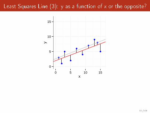
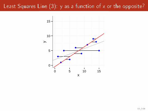
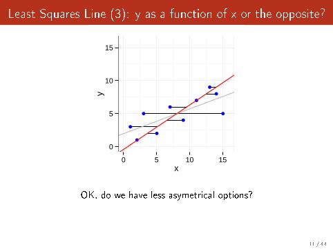
Least Squares Line (3): y as a function of x or the opposite?
●
●
●
●
●
●
●
●
●
●
0
5
10
15
0 5 10 15x
y
OK, do we have less asymetrical options?
11 / 44
Least Squares Line (3): y as a function of x or the opposite?
●
●
●
●
●
●
●
●
●
●
0
5
10
15
0 5 10 15x
y
OK, do we have less asymetrical options?
11 / 44
Least Squares Line (3): y as a function of x or the opposite?
●
●
●
●
●
●
●
●
●
●
0
5
10
15
0 5 10 15x
y
OK, do we have less asymetrical options?
11 / 44
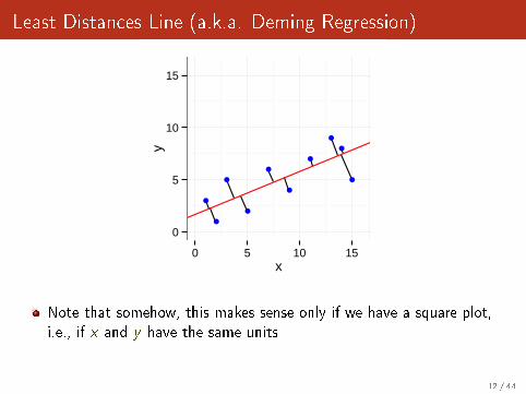
Least Distances Line (a.k.a. Deming Regression)
●
●
●
●
●
●
●
●
●
●
0
5
10
15
0 5 10 15x
y
Note that somehow, this makes sense only if we have a square plot,i.e., if x and y have the same units
12 / 44
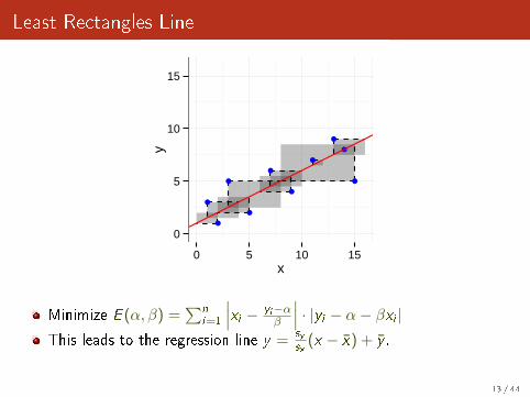
Least Rectangles Line
●
●
●
●
●
●
●
●
●
●
0
5
10
15
0 5 10 15x
y
Minimize E (α, β) =∑n
i=1
∣∣∣xi − yi−αβ
∣∣∣ · |yi − α− βxi |This leads to the regression line y =
sysx
(x − x) + y .
13 / 44
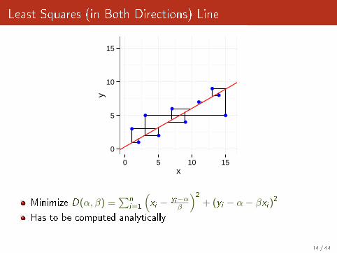
Least Squares (in Both Directions) Line
●
●
●
●
●
●
●
●
●
●
0
5
10
15
0 5 10 15x
y
Minimize D(α, β) =∑n
i=1
(xi − yi−α
β
)2+ (yi − α− βxi )2
Has to be computed analytically
14 / 44
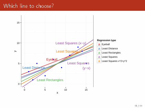
Which line to choose?
●
●
●
●
●
●
●
●
●
●Least Squares
(y~x)
Least Squares (x~y)
Least Squares
Least Distance
Least Rectangles
Eyeball
0
5
10
15
0 5 10 15x
y
Regression type
aaaaa
Eyeball
Least Distance
Least Rectangles
Least Squares
Least Squares x^2+y^2
15 / 44
What does correspond to each line?
Eyeball: AFAIK nothing
Least Squares: classical linear regression y ∼ x
Least Squares in both directions: I don't know
Deming: equivalent to Principal Component Analysis
Rectangles: may be used when one variable is not "explained" by theother, but are inter-dependent
This is not just a geometric problem. You need a model of to decide whichone to use
16 / 44
Outline
1 Simple Linear RegressionGeneral IntroductionFitting a Line to a Set of Points
2 Linear ModelLinear RegressionUnderlying HypothesisChecking hypothesisDecomposing the VarianceMaking PredictionsCon�dence interval
3 Conclusion
17 / 44
Outline
1 Simple Linear RegressionGeneral IntroductionFitting a Line to a Set of Points
2 Linear ModelLinear RegressionUnderlying HypothesisChecking hypothesisDecomposing the VarianceMaking PredictionsCon�dence interval
3 Conclusion
18 / 44
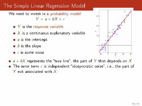
The Simple Linear Regression Model
We need to invest in a probability modelY = a + bX + ε
Y is the response variable
X is a continuous explanatory variable
a is the intercept
b is the slope
ε is some noise
●
●
●
●
●
●
●
●
●
●
●
●
●
●
●
●
●
●
●
●
●
●
●
●
●
●
●
●
●
●
●
●
●
●
●
●
●
●
●
●
●
●
●
●
●
●
●●
●
●
0
10
20
30
−20 0 20 40 60x
y
a + bX represents the �true line�, the part of Y that depends on X
The error term ε is independent �idosyncratic noise�, i.e., the part ofY not associated with X
Gauss-Markov Theorem
Under a few assumptions, the least squares regression is the best linearunbiased estimate
E(β) = b and E(α) = a Var(β) and Var(α) are minimal
19 / 44
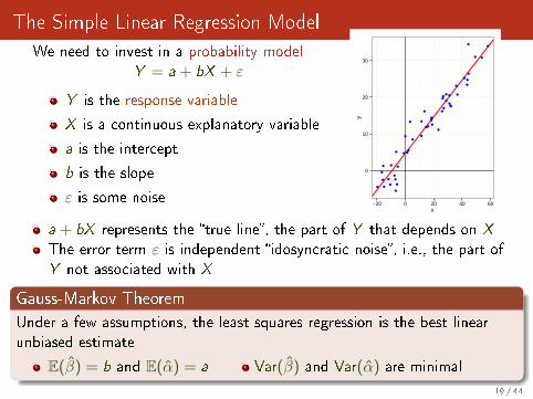
Multiple explanatory variables
The same results hold true when there are several explanatoryvariables:
Y = a + b(1)X (1) + b(2)X (2) + b(1,2)X (1)X (2) + ε
The least squares regressions are good estimators of a, b(1), b(2),b(1,2)
We can use an arbitrary linear combination of variables, hence
Y = a + b(1)X + b(2) 1X
+ b(3)X 3 + ε
is also a linear model
Obviously the closed-form formula are much more complicated butsoftwares like R handle this very well
20 / 44

Outline
1 Simple Linear RegressionGeneral IntroductionFitting a Line to a Set of Points
2 Linear ModelLinear RegressionUnderlying HypothesisChecking hypothesisDecomposing the VarianceMaking PredictionsCon�dence interval
3 Conclusion
21 / 44
Important Hypothesis (1)
Weak exogeneity The predictor variables X can be treated as �xed values,rather than random variables: the X are assumed to be error-free, i.e.,they are not contaminated with measurement errorsAlthough not realistic in many settings, dropping this assumption leadsto signi�cantly more di�cult errors-in-variables models
Linearity the mean of the response variable is a linear combination of theparameters (regression coe�cients) and the predictor variablesSince predictor variables themselves can be arbitrarily transformed, thisis not that restrictive. This trick is used, for example, in polynomialregression, but beware of over�tting
Independance of Errors if several responses Y1 and Y2 are �t, ε1 and ε2should be independant
22 / 44
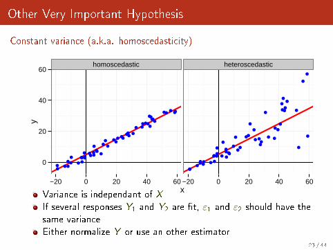
Other Very Important Hypothesis
Constant variance (a.k.a. homoscedasticity)
●
●●
●
●
●
●●
●●
●
●
● ●
●●
●
●
●
●
●
●
●
●
●
●
●
●
●
●
●
●
●
●
●
●
●
●
●
●
●
●
●
●
●
●
●
●
●●
●
●
●
●
●
●
●
●
●
●
●●
● ●●
●
●
●
●
●
●
●
●
●●
●
●
●
●
● ●
●
●
●
●
●
●
●
●
●
●
●
●
●
●
●●
●
●
●
homoscedastic heteroscedastic
0
20
40
60
−20 0 20 40 60 −20 0 20 40 60x
y
Variance is independant of XIf several responses Y1 and Y2 are �t, ε1 and ε2 should have thesame varianceEither normalize Y or use an other estimator
23 / 44
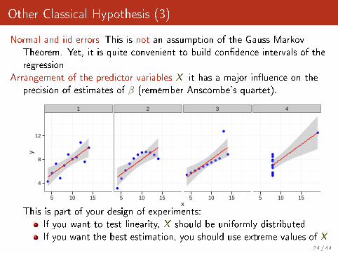
Other Classical Hypothesis (3)
Normal and iid errors This is not an assumption of the Gauss MarkovTheorem. Yet, it is quite convenient to build con�dence intervals of theregression
Arrangement of the predictor variables X it has a major in�uence on theprecision of estimates of β (remember Anscombe's quartet).
●
●●
●●
●
●
●
●
●
●
●
●●●
●
●
●
●
●
●
●
●
●
●
●
●
●
●
●
●
●
●
●
●
●
●●
●
●
●
●
●
●
1 2 3 4
4
8
12
5 10 15 5 10 15 5 10 15 5 10 15x
y
This is part of your design of experiments:If you want to test linearity, X should be uniformly distributedIf you want the best estimation, you should use extreme values of X
24 / 44
Outline
1 Simple Linear RegressionGeneral IntroductionFitting a Line to a Set of Points
2 Linear ModelLinear RegressionUnderlying HypothesisChecking hypothesisDecomposing the VarianceMaking PredictionsCon�dence interval
3 Conclusion
25 / 44
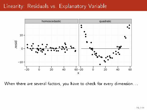
Linearity: Residuals vs. Explanatory Variable
●●
●
● ●
●
●●
●
●
●
●
●
●●●
●
●●
●●
●
●
●●
● ● ● ●●
●
●●
●
●●
●
●●
●
●●●
●
●
●
●●
●●
●
●●
●
●
●
●
●
●●
●●
●●
●
●
●
●
●●
●
●
●
●
●
●
●
●
●
●
●
●
●
●
●
●
●
●
●
●
●●
●
●
●
●
●
●
●
●
homoscedastic quadratic
−10
0
10
−20 0 20 40 60 −20 0 20 40 60x
.res
id
When there are several factors, you have to check for every dimension. . .
26 / 44
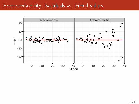
Homoscedasticity: Residuals vs. Fitted values
●●
●
● ●●
●●
●●
●
●●
●●●
●● ●
● ●
●●
● ●● ● ● ●●
●
●●●
●●
●
●●●
●●●
●●
●
●●
●●
●●● ●
●
●
●
●
●
●
●
●
●
●
●
●
●
●
●
●
●
●
●
●
●●
●
●
●
●
●
●
●
●
●
●
●
●
●●
●
●●
●
●
●
●
●
●
●
homoscedastic heteroscedastic
−20
−10
0
10
20
0 10 20 30 40 0 10 20 30 40.fitted
.res
id
27 / 44
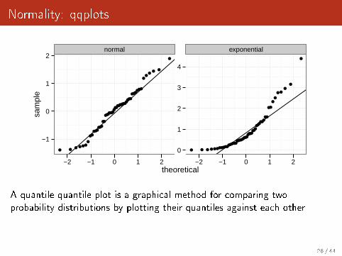
Normality: qqplots
● ● ● ●●●●
●●●●●
●●●●●
●●●●●●●
●●●
●●●●●●●●
●●●●●●
●●●
●●
●● ●
●
● ● ● ●●●●●●●●●●●●●●
●●●●●●●●●
●●●●●●
●●●
●●●●●●
●●
●●
●●●
●
●
normal exponential
−1
0
1
2
0
1
2
3
4
−2 −1 0 1 2 −2 −1 0 1 2theoretical
sam
ple
A quantile-quantile plot is a graphical method for comparing twoprobability distributions by plotting their quantiles against each other
28 / 44
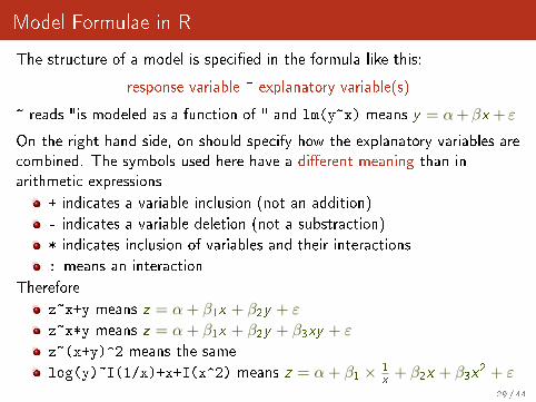
Model Formulae in R
The structure of a model is speci�ed in the formula like this:
response variable ~ explanatory variable(s)
~ reads "is modeled as a function of " and lm(y~x) means y = α+βx + ε
On the right-hand side, on should specify how the explanatory variables arecombined. The symbols used here have a di�erent meaning than inarithmetic expressions
+ indicates a variable inclusion (not an addition)
- indicates a variable deletion (not a substraction)
* indicates inclusion of variables and their interactions
: means an interaction
Therefore
z~x+y means z = α + β1x + β2y + ε
z~x*y means z = α + β1x + β2y + β3xy + ε
z~(x+y)^2 means the same
log(y)~I(1/x)+x+I(x^2) means z = α + β1 × 1x
+ β2x + β3x2 + ε
29 / 44
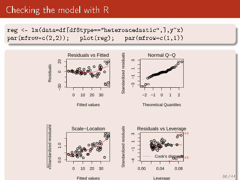
Checking the model with R
reg <- lm(data=df[df$type=="heteroscedastic",],y~x)
par(mfrow=c(2,2)); plot(reg); par(mfrow=c(1,1))
0 10 20 30
−30
020
Fitted values
Res
idua
ls
●●● ●
●
●
●
●●
●
●●
●●
●
●
●
●
●●
●●
●
●
●● ●
●
●
●●
●
●
●●
●
●
●
●●●
● ●●
●
●
●
●
●
●
Residuals vs Fitted
8265
66
●●●●
●
●
●
●●
●
●●
●●
●
●
●
●
●●
●●
●
●
●●●
●
●
●●
●
●
●●
●
●
●
●●●
●●●
●
●
●
●
●
●
−2 −1 0 1 2
−3
−1
13
Theoretical Quantiles
Sta
ndar
dize
d re
sidu
als Normal Q−Q
8265
66
0 10 20 30
0.0
1.0
Fitted values
Sta
ndar
dize
d re
sidu
als
●●● ●
●
●
●
●
●
●
●
●
●●
●●
●
●
●
●
●
●
●●●
●
●
●●
●
●
●
●
●
●
●
●
●
●●
●
●●
●
●●
●
●
●●
Scale−Location82
6566
0.00 0.04 0.08
−4
−1
13
Leverage
Sta
ndar
dize
d re
sidu
als
● ● ●●
●
●
●
●●
●
●●
●●
●
●
●
●
●●
●●
●
●
● ●●
●
●
●●
●
●
●●
●
●
●
● ●●
●●●
●
●
●
●
●
●
Cook's distance 0.5
0.5Residuals vs Leverage
8265
66
30 / 44
Outline
1 Simple Linear RegressionGeneral IntroductionFitting a Line to a Set of Points
2 Linear ModelLinear RegressionUnderlying HypothesisChecking hypothesisDecomposing the VarianceMaking PredictionsCon�dence interval
3 Conclusion
31 / 44
Decomposing the Variance
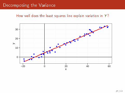
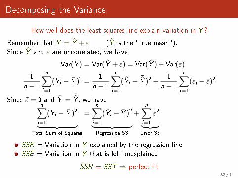
How well does the least squares line explain variation in Y ?
●
●●
●
●
●
●
●
●
●
●
●
● ●
●●
●
●
●
●
●
●
●
●
●
●
●
●
●
●
●
●
●
●
●
●
●
●
●
●
●
●
●
●
●
●
●
●
●
●
0
10
20
30
−20 0 20 40 60x
y
Remember that Y = Y + ε (Y is the "true mean").Since Y and ε are uncorrelated, we have
Var(Y ) = Var(Y + ε) = Var(Y ) + Var(ε)
1
n − 1
n∑i=1
(Yi − Y )2 =1
n − 1
n∑i=1
(Yi − ¯Y )2 +
1
n − 1
n∑i=1
(εi − ε)2
Since ε = 0 and Y = ¯Y , we have
n∑i=1
(Yi − Y )2︸ ︷︷ ︸Total Sum of Squares
=n∑
i=1
(Yi − Y )2︸ ︷︷ ︸Regression SS
+n∑
i=1
ε2︸ ︷︷ ︸Error SS
SSR = Variation in Y explained by the regression lineSSE = Variation in Y that is left unexplained
SSR = SST ⇒ perfect �t
32 / 44
Decomposing the Variance
How well does the least squares line explain variation in Y ?
Remember that Y = Y + ε (Y is the "true mean").Since Y and ε are uncorrelated, we have
Var(Y ) = Var(Y + ε) = Var(Y ) + Var(ε)
1
n − 1
n∑i=1
(Yi − Y )2 =1
n − 1
n∑i=1
(Yi − ¯Y )2 +
1
n − 1
n∑i=1
(εi − ε)2
Since ε = 0 and Y = ¯Y , we have
n∑i=1
(Yi − Y )2︸ ︷︷ ︸Total Sum of Squares
=n∑
i=1
(Yi − Y )2︸ ︷︷ ︸Regression SS
+n∑
i=1
ε2︸ ︷︷ ︸Error SS
SSR = Variation in Y explained by the regression lineSSE = Variation in Y that is left unexplained
SSR = SST ⇒ perfect �t32 / 44
A Goodness of Fit Measure: R2
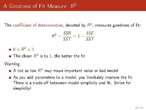
The coe�cient of determination, denoted by R2, measures goodness of �t:
R2 =SSR
SST= 1− SSE
SST
0 6 R2 6 1
The closer R2 is to 1, the better the �t
Warning:
A not so low R2 may mean important noise or bad model
As you add parameters to a model, you inevitably improve the �t.There is a trade-o� beteween model simplicity and �t. Strive forsimplicity!
33 / 44
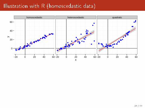
Illustration with R (homoscedastic data)
●
●●
●
●
●
●●
●●
●
●
● ●
●●
●
●
●
●
●
●
●
●
●
●
●
●
●
●
●
●
●
●
●
●
●●
●
●
●
●
●
●
●
●
●
●
●●
●
●●
●
●
●
●
●
●
●
●●
● ● ●
●
●
●
●
●
●
●
●
●●
●
●
●●
● ●
●
●
●
●
●
●
●
●
●
●
●
●
●
●
●●
●
●
●
●●
●
●
●
●
●
●
●
●
● ●
●●
●●
●
●
●
●
●●
●
● ●● ●
●
●
●●
●
●
●
●●
●
●
●
●
●
●
●●
●●
●
●
●
●
homoscedastic heteroscedastic quadratic
0
20
40
60
−20 0 20 40 60−20 0 20 40 60−20 0 20 40 60x
y
reg <- lm(data=df[df$type=="homoscedastic",],y~x)
summary(reg)
Call:
lm(formula = y ~ x, data = df[df$type == "homoscedastic", ])
Residuals:
Min 1Q Median 3Q Max
-4.1248 -1.3059 -0.0366 1.0588 3.9965
Coefficients:
Estimate Std. Error t value Pr(>|t|)
(Intercept) 4.56481 0.33165 13.76 <2e-16 ***
x 0.50645 0.01154 43.89 <2e-16 ***
---
Signif. codes: 0 `***' 0.001 `**' 0.01 `*' 0.05 `.' 0.1 ` ' 1
Residual standard error: 1.816 on 48 degrees of freedom
Multiple R-squared: 0.9757, Adjusted R-squared: 0.9752
F-statistic: 1926 on 1 and 48 DF, p-value: < 2.2e-16
34 / 44
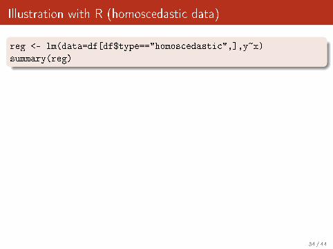
Illustration with R (homoscedastic data)
reg <- lm(data=df[df$type=="homoscedastic",],y~x)
summary(reg)
Call:
lm(formula = y ~ x, data = df[df$type == "homoscedastic", ])
Residuals:
Min 1Q Median 3Q Max
-4.1248 -1.3059 -0.0366 1.0588 3.9965
Coefficients:
Estimate Std. Error t value Pr(>|t|)
(Intercept) 4.56481 0.33165 13.76 <2e-16 ***
x 0.50645 0.01154 43.89 <2e-16 ***
---
Signif. codes: 0 `***' 0.001 `**' 0.01 `*' 0.05 `.' 0.1 ` ' 1
Residual standard error: 1.816 on 48 degrees of freedom
Multiple R-squared: 0.9757, Adjusted R-squared: 0.9752
F-statistic: 1926 on 1 and 48 DF, p-value: < 2.2e-16
34 / 44
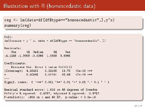
Illustration with R (homoscedastic data)
reg <- lm(data=df[df$type=="homoscedastic",],y~x)
summary(reg)
Call:
lm(formula = y ~ x, data = df[df$type == "homoscedastic", ])
Residuals:
Min 1Q Median 3Q Max
-4.1248 -1.3059 -0.0366 1.0588 3.9965
Coefficients:
Estimate Std. Error t value Pr(>|t|)
(Intercept) 4.56481 0.33165 13.76 <2e-16 ***
x 0.50645 0.01154 43.89 <2e-16 ***
---
Signif. codes: 0 `***' 0.001 `**' 0.01 `*' 0.05 `.' 0.1 ` ' 1
Residual standard error: 1.816 on 48 degrees of freedom
Multiple R-squared: 0.9757, Adjusted R-squared: 0.9752
F-statistic: 1926 on 1 and 48 DF, p-value: < 2.2e-16
34 / 44

Illustration with R (heteroscedastic data)
●
●●
●
●
●
●●
●●
●
●
● ●
●●
●
●
●
●
●
●
●
●
●
●
●
●
●
●
●
●
●
●
●
●
●●
●
●
●
●
●
●
●
●
●
●
●●
●
●●
●
●
●
●
●
●
●
●●
● ● ●
●
●
●
●
●
●
●
●
●●
●
●
●●
● ●
●
●
●
●
●
●
●
●
●
●
●
●
●
●
●●
●
●
●
●●
●
●
●
●
●
●
●
●
● ●
●●
●●
●
●
●
●
●●
●
● ●● ●
●
●
●●
●
●
●
●●
●
●
●
●
●
●
●●
●●
●
●
●
●
homoscedastic heteroscedastic quadratic
0
20
40
60
−20 0 20 40 60−20 0 20 40 60−20 0 20 40 60x
y
reg <- lm(data=df[df$type=="heteroscedastic",],y~x)
summary(reg)
Call:
lm(formula = y ~ x, data = df[df$type == "heteroscedastic", ])
Residuals:
Min 1Q Median 3Q Max
-25.063 -3.472 0.663 3.707 19.327
Coefficients:
Estimate Std. Error t value Pr(>|t|)
(Intercept) 4.98800 1.41061 3.536 0.000911 ***
x 0.56002 0.04908 11.411 2.83e-15 ***
---
Signif. codes: 0 `***' 0.001 `**' 0.01 `*' 0.05 `.' 0.1 ` ' 1
Residual standard error: 7.722 on 48 degrees of freedom
Multiple R-squared: 0.7306, Adjusted R-squared: 0.725
F-statistic: 130.2 on 1 and 48 DF, p-value: 2.83e-15
35 / 44
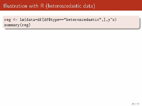
Illustration with R (heteroscedastic data)
reg <- lm(data=df[df$type=="heteroscedastic",],y~x)
summary(reg)
Call:
lm(formula = y ~ x, data = df[df$type == "heteroscedastic", ])
Residuals:
Min 1Q Median 3Q Max
-25.063 -3.472 0.663 3.707 19.327
Coefficients:
Estimate Std. Error t value Pr(>|t|)
(Intercept) 4.98800 1.41061 3.536 0.000911 ***
x 0.56002 0.04908 11.411 2.83e-15 ***
---
Signif. codes: 0 `***' 0.001 `**' 0.01 `*' 0.05 `.' 0.1 ` ' 1
Residual standard error: 7.722 on 48 degrees of freedom
Multiple R-squared: 0.7306, Adjusted R-squared: 0.725
F-statistic: 130.2 on 1 and 48 DF, p-value: 2.83e-15
35 / 44
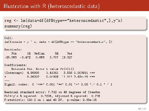
Illustration with R (heteroscedastic data)
reg <- lm(data=df[df$type=="heteroscedastic",],y~x)
summary(reg)
Call:
lm(formula = y ~ x, data = df[df$type == "heteroscedastic", ])
Residuals:
Min 1Q Median 3Q Max
-25.063 -3.472 0.663 3.707 19.327
Coefficients:
Estimate Std. Error t value Pr(>|t|)
(Intercept) 4.98800 1.41061 3.536 0.000911 ***
x 0.56002 0.04908 11.411 2.83e-15 ***
---
Signif. codes: 0 `***' 0.001 `**' 0.01 `*' 0.05 `.' 0.1 ` ' 1
Residual standard error: 7.722 on 48 degrees of freedom
Multiple R-squared: 0.7306, Adjusted R-squared: 0.725
F-statistic: 130.2 on 1 and 48 DF, p-value: 2.83e-15
35 / 44
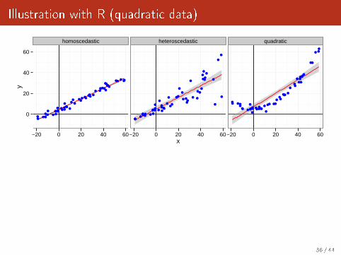
Illustration with R (quadratic data)
●
●●
●
●
●
●●
●●
●
●
● ●
●●
●
●
●
●
●
●
●
●
●
●
●
●
●
●
●
●
●
●
●
●
●●
●
●
●
●
●
●
●
●
●
●
●●
●
●●
●
●
●
●
●
●
●
●●
● ● ●
●
●
●
●
●
●
●
●
●●
●
●
●●
● ●
●
●
●
●
●
●
●
●
●
●
●
●
●
●
●●
●
●
●
●●
●
●
●
●
●
●
●
●
● ●
●●
●●
●
●
●
●
●●
●
● ●● ●
●
●
●●
●
●
●
●●
●
●
●
●
●
●
●●
●●
●
●
●
●
homoscedastic heteroscedastic quadratic
0
20
40
60
−20 0 20 40 60−20 0 20 40 60−20 0 20 40 60x
y
reg <- lm(data=df[df$type=="quadratic",],y~x)
summary(reg)
Call:
lm(formula = y ~ x, data = df[df$type == "quadratic", ])
Residuals:
Min 1Q Median 3Q Max
-11.759 -5.847 -2.227 3.746 17.346
Coefficients:
Estimate Std. Error t value Pr(>|t|)
(Intercept) 7.05330 1.41238 4.994 8.23e-06 ***
x 0.65517 0.04914 13.333 < 2e-16 ***
---
Signif. codes: 0 `***' 0.001 `**' 0.01 `*' 0.05 `.' 0.1 ` ' 1
Residual standard error: 7.732 on 48 degrees of freedom
Multiple R-squared: 0.7874, Adjusted R-squared: 0.783
F-statistic: 177.8 on 1 and 48 DF, p-value: < 2.2e-16
36 / 44
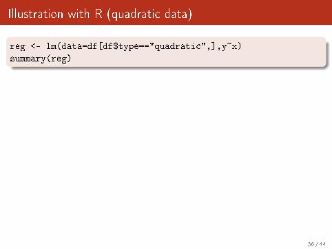
Illustration with R (quadratic data)
reg <- lm(data=df[df$type=="quadratic",],y~x)
summary(reg)
Call:
lm(formula = y ~ x, data = df[df$type == "quadratic", ])
Residuals:
Min 1Q Median 3Q Max
-11.759 -5.847 -2.227 3.746 17.346
Coefficients:
Estimate Std. Error t value Pr(>|t|)
(Intercept) 7.05330 1.41238 4.994 8.23e-06 ***
x 0.65517 0.04914 13.333 < 2e-16 ***
---
Signif. codes: 0 `***' 0.001 `**' 0.01 `*' 0.05 `.' 0.1 ` ' 1
Residual standard error: 7.732 on 48 degrees of freedom
Multiple R-squared: 0.7874, Adjusted R-squared: 0.783
F-statistic: 177.8 on 1 and 48 DF, p-value: < 2.2e-16
36 / 44
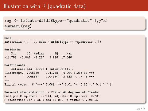
Illustration with R (quadratic data)
reg <- lm(data=df[df$type=="quadratic",],y~x)
summary(reg)
Call:
lm(formula = y ~ x, data = df[df$type == "quadratic", ])
Residuals:
Min 1Q Median 3Q Max
-11.759 -5.847 -2.227 3.746 17.346
Coefficients:
Estimate Std. Error t value Pr(>|t|)
(Intercept) 7.05330 1.41238 4.994 8.23e-06 ***
x 0.65517 0.04914 13.333 < 2e-16 ***
---
Signif. codes: 0 `***' 0.001 `**' 0.01 `*' 0.05 `.' 0.1 ` ' 1
Residual standard error: 7.732 on 48 degrees of freedom
Multiple R-squared: 0.7874, Adjusted R-squared: 0.783
F-statistic: 177.8 on 1 and 48 DF, p-value: < 2.2e-16
36 / 44
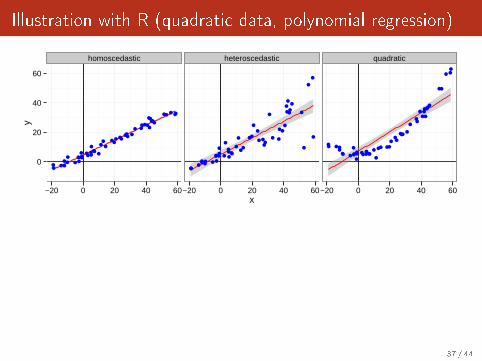
Illustration with R (quadratic data, polynomial regression)
●
●●
●
●
●
●●
●●
●
●
● ●
●●
●
●
●
●
●
●
●
●
●
●
●
●
●
●
●
●
●
●
●
●
●●
●
●
●
●
●
●
●
●
●
●
●●
●
●●
●
●
●
●
●
●
●
●●
● ● ●
●
●
●
●
●
●
●
●
●●
●
●
●●
● ●
●
●
●
●
●
●
●
●
●
●
●
●
●
●
●●
●
●
●
●●
●
●
●
●
●
●
●
●
● ●
●●
●●
●
●
●
●
●●
●
● ●● ●
●
●
●●
●
●
●
●●
●
●
●
●
●
●
●●
●●
●
●
●
●
homoscedastic heteroscedastic quadratic
0
20
40
60
−20 0 20 40 60−20 0 20 40 60−20 0 20 40 60x
y
df$x2=df$x^2
reg_quad <- lm(data=df[df$type=="quadratic",],y~x+x2)
summary(reg_quad)
Call:
lm(formula = y ~ x + x2, data = df[df$type == "quadratic", ])
Residuals:
Min 1Q Median 3Q Max
-4.7834 -0.8638 -0.0480 1.1312 3.9913
Coefficients:
Estimate Std. Error t value Pr(>|t|)
(Intercept) 5.3065389 0.3348067 15.850 <2e-16 ***
x 0.0036098 0.0252807 0.143 0.887
x2 0.0164635 0.0005694 28.913 <2e-16 ***
---
Signif. codes: 0 `***' 0.001 `**' 0.01 `*' 0.05 `.' 0.1 ` ' 1
Residual standard error: 1.803 on 47 degrees of freedom
Multiple R-squared: 0.9887, Adjusted R-squared: 0.9882
F-statistic: 2053 on 2 and 47 DF, p-value: < 2.2e-16
37 / 44
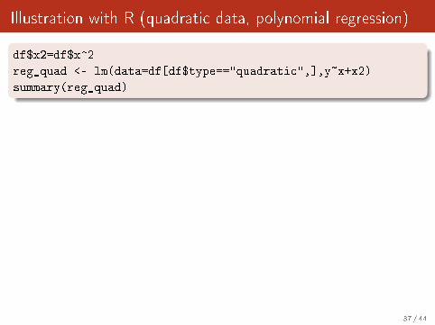
Illustration with R (quadratic data, polynomial regression)
df$x2=df$x^2
reg_quad <- lm(data=df[df$type=="quadratic",],y~x+x2)
summary(reg_quad)
Call:
lm(formula = y ~ x + x2, data = df[df$type == "quadratic", ])
Residuals:
Min 1Q Median 3Q Max
-4.7834 -0.8638 -0.0480 1.1312 3.9913
Coefficients:
Estimate Std. Error t value Pr(>|t|)
(Intercept) 5.3065389 0.3348067 15.850 <2e-16 ***
x 0.0036098 0.0252807 0.143 0.887
x2 0.0164635 0.0005694 28.913 <2e-16 ***
---
Signif. codes: 0 `***' 0.001 `**' 0.01 `*' 0.05 `.' 0.1 ` ' 1
Residual standard error: 1.803 on 47 degrees of freedom
Multiple R-squared: 0.9887, Adjusted R-squared: 0.9882
F-statistic: 2053 on 2 and 47 DF, p-value: < 2.2e-16
37 / 44
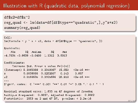
Illustration with R (quadratic data, polynomial regression)
df$x2=df$x^2
reg_quad <- lm(data=df[df$type=="quadratic",],y~x+x2)
summary(reg_quad)
Call:
lm(formula = y ~ x + x2, data = df[df$type == "quadratic", ])
Residuals:
Min 1Q Median 3Q Max
-4.7834 -0.8638 -0.0480 1.1312 3.9913
Coefficients:
Estimate Std. Error t value Pr(>|t|)
(Intercept) 5.3065389 0.3348067 15.850 <2e-16 ***
x 0.0036098 0.0252807 0.143 0.887
x2 0.0164635 0.0005694 28.913 <2e-16 ***
---
Signif. codes: 0 `***' 0.001 `**' 0.01 `*' 0.05 `.' 0.1 ` ' 1
Residual standard error: 1.803 on 47 degrees of freedom
Multiple R-squared: 0.9887, Adjusted R-squared: 0.9882
F-statistic: 2053 on 2 and 47 DF, p-value: < 2.2e-1637 / 44
Outline
1 Simple Linear RegressionGeneral IntroductionFitting a Line to a Set of Points
2 Linear ModelLinear RegressionUnderlying HypothesisChecking hypothesisDecomposing the VarianceMaking PredictionsCon�dence interval
3 Conclusion
38 / 44
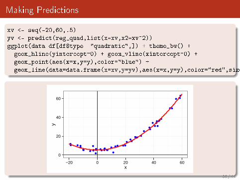
Making Predictions
xv <- seq(-20,60,.5)
yv <- predict(reg_quad,list(x=xv,x2=xv^2))
ggplot(data=df[df$type=="quadratic",]) + theme_bw() +
geom_hline(yintercept=0) + geom_vline(xintercept=0) +
geom_point(aes(x=x,y=y),color="blue") +
geom_line(data=data.frame(x=xv,y=yv),aes(x=x,y=y),color="red",size=1)
●●
●
●
●
●
●
●
●
●
● ●
●
●
●●
●
●
●
●
●●
●
● ●● ●
●
●
●●
●
●
●
●
●
●
●
●
●
●
●
●●
●●
●
●
●
●
0
20
40
60
−20 0 20 40 60x
y
39 / 44
Outline
1 Simple Linear RegressionGeneral IntroductionFitting a Line to a Set of Points
2 Linear ModelLinear RegressionUnderlying HypothesisChecking hypothesisDecomposing the VarianceMaking PredictionsCon�dence interval
3 Conclusion
40 / 44
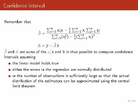
Con�dence interval
Remember that
β =
∑ni=1 xiyi −
1n
∑ni=1 xi
∑nj=1 yj∑n
i=1(x2i )− 1n
(∑n
i=1 xi )2
α = y − β xβ and α are sums of the εi 's and it is thus possible to compute con�denceintervals assuming:
the linear model holds true
either the errors in the regression are normally distributed
or the number of observations is su�ciently large so that the actualdistribution of the estimators can be approximated using the centrallimit theorem
41 / 44
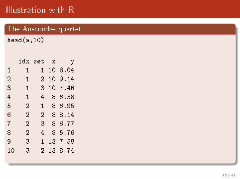
Illustration with R
The Anscombe quartet
head(a,10)
idx set x y
1 1 1 10 8.04
2 1 2 10 9.14
3 1 3 10 7.46
4 1 4 8 6.58
5 2 1 8 6.95
6 2 2 8 8.14
7 2 3 8 6.77
8 2 4 8 5.76
9 3 1 13 7.58
10 3 2 13 8.74
Con�dence intervals with ggplot
ggplot(data=a,aes(x=x,y=y)) + theme_bw() +
facet_wrap(~set,nrow=1) + geom_point(color="blue") +
geom_smooth(method='lm',color="red")
●
●●
●●
●
●
●
●
●
●
●
●●●
●
●
●
●
●
●
●
●
●
●
●
●
●
●
●
●
●
●
●
●
●
●●
●
●
●
●
●
●
1 2 3 4
4
8
12
5 10 15 5 10 15 5 10 15 5 10 15x
y
●
●●
●●
●
●
●
●
●
●
●
●●●
●
●
●
●
●
●
●
●
●
●
●
●
●
●
●
●
●
●
●
●
●
●●
●
●
●
●
●
●
1 2 3 4
4
8
12
5 10 15 5 10 15 5 10 15 5 10 15x
y
42 / 44
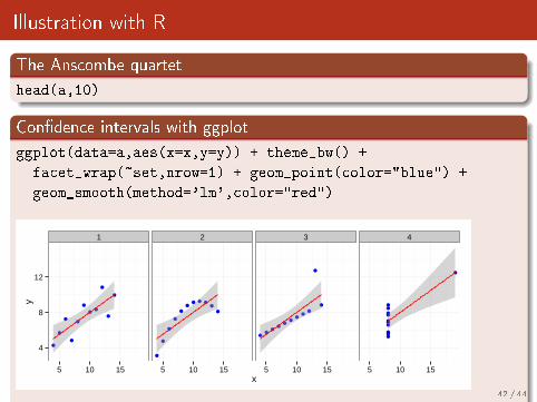
Illustration with R
The Anscombe quartet
head(a,10)
Con�dence intervals with ggplot
ggplot(data=a,aes(x=x,y=y)) + theme_bw() +
facet_wrap(~set,nrow=1) + geom_point(color="blue") +
geom_smooth(method='lm',color="red")
●
●●
●●
●
●
●
●
●
●
●
●●●
●
●
●
●
●
●
●
●
●
●
●
●
●
●
●
●
●
●
●
●
●
●●
●
●
●
●
●
●
1 2 3 4
4
8
12
5 10 15 5 10 15 5 10 15 5 10 15x
y
●
●●
●●
●
●
●
●
●
●
●
●●●
●
●
●
●
●
●
●
●
●
●
●
●
●
●
●
●
●
●
●
●
●
●●
●
●
●
●
●
●
1 2 3 4
4
8
12
5 10 15 5 10 15 5 10 15 5 10 15x
y
42 / 44
Outline
1 Simple Linear RegressionGeneral IntroductionFitting a Line to a Set of Points
2 Linear ModelLinear RegressionUnderlying HypothesisChecking hypothesisDecomposing the VarianceMaking PredictionsCon�dence interval
3 Conclusion
43 / 44
Conclusion
1 You need a model to perform your regression
2 You need to check whether the underlying hypothesis of this model arereasonable or not
This model will allow you to:
1 Assess and quantify the e�ect of parameters on the response
2 Extrapolate within the range of parameters you tried
3 Detect outstanding points (those with a high residual and/or with ahigh lever)
This model will guide on how to design your experiments:
e.g., the linear model assumes some uniformity of interest over theparameter space range
if your system is heteroscedastic, you will have to perform moremeasurements for parameters that lead to higher variance
44 / 44
Recommended


