Introduction to Kohn–Sham density-functional theory
Introduction to Kohn–Sham density-functional theory
Emmanuel Fromager
Institut de Chimie de Strasbourg - Laboratoire de Chimie Quantique -Université de Strasbourg /CNRS
EUR: Theory of extended systems
Institut de Chimie, Strasbourg, France Page 1
Introduction to Kohn–Sham density-functional theory
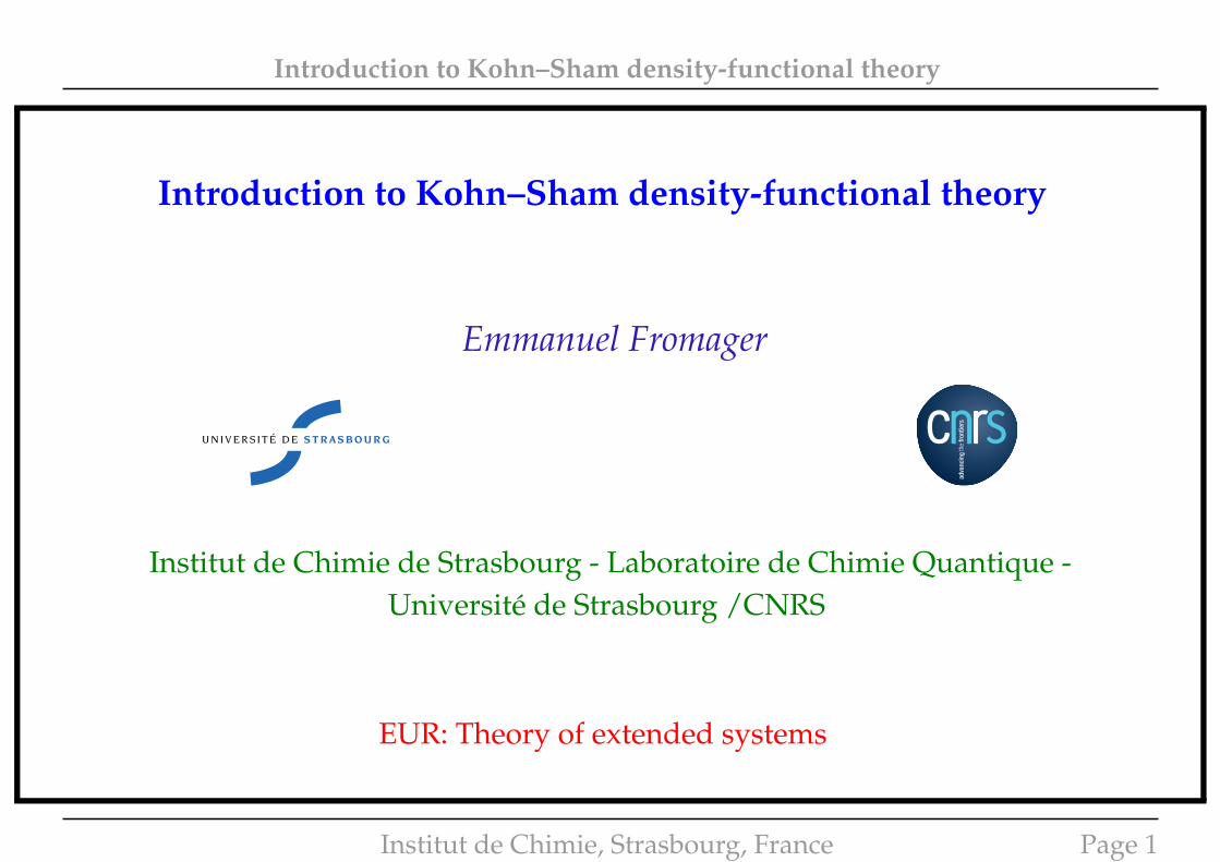
N -electron Schrödinger equation for the ground state
HΨ0 = E0Ψ0
where Ψ0 ≡ Ψ0(x1,x2, . . . ,xN ), xi ≡ (ri, σi) ≡ (xi, yi, zi, σi = ± 12
) for i = 1, 2, . . . , N,
and H = T + Wee + V .
T ≡ −1
2
N∑i=1
∇2ri
= −1
2
N∑i=1
(∂2
∂x2i
+∂2
∂y2i
+∂2
∂z2i
)−→ universal kinetic energy operator
Wee ≡N∑i<j
1
|ri − rj |× −→ universal two-electron repulsion operator
V ≡N∑i=1
v(ri)× where v(r) = −nuclei∑A
ZA
|r−RA|−→ local nuclear potential operator
Institut de Chimie, Strasbourg, France Page 2
Introduction to Kohn–Sham density-functional theory
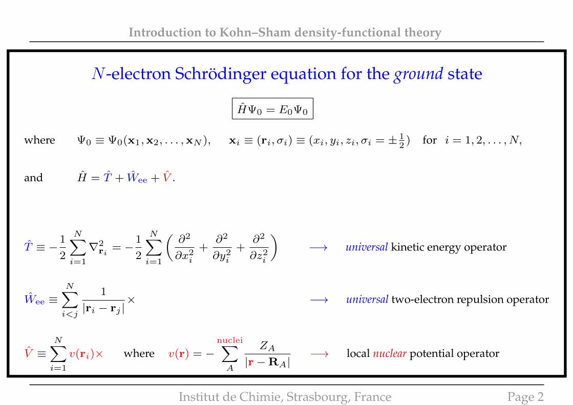
(Fictitious) non-interacting electrons• Solving the Schrödinger equation for non-interacting electrons is easy.
• You “just" have to solve the Schrödinger equation for a single electron.
(T +
N∑i=1
v(ri)×)
Φ0 = E0Φ0 ⇔[−
1
2∇2
r + v(r)×]ϕi(x) = εiϕi(x), i = 1, 2, . . . , N.
Proof: a simple solution to the N -electron non-interacting Schrödinger equation is
Φ0 ≡ ϕ1(x1)× ϕ2(x2)× . . .× ϕN (xN ) =
N∏j=1
ϕj(xj) ← Hartree product!
since(T +
N∑i=1
v(ri)×)
Φ0 =N∑i=1
N∏j 6=i
ϕj(xj)×[−
1
2∇2
ri+ v(ri)×
]ϕi(xi) =
(N∑i=1
εi
)Φ0.
Institut de Chimie, Strasbourg, France Page 3
Introduction to Kohn–Sham density-functional theory
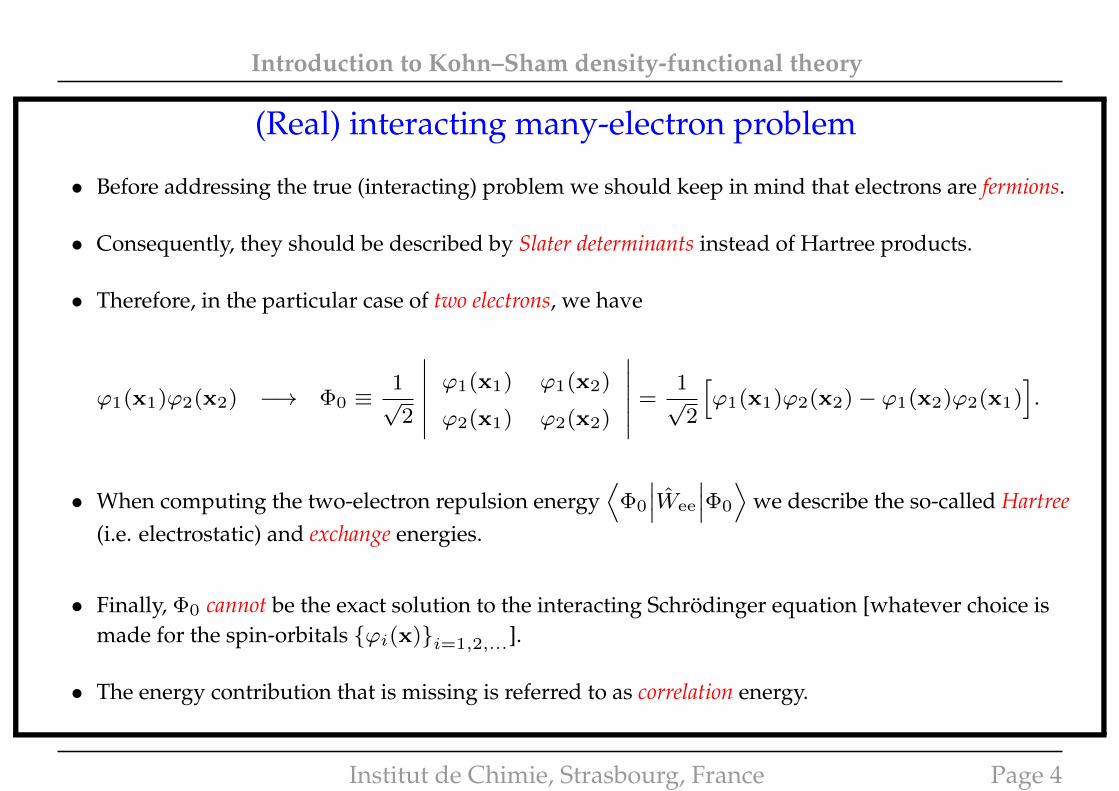
(Real) interacting many-electron problem
• Before addressing the true (interacting) problem we should keep in mind that electrons are fermions.
• Consequently, they should be described by Slater determinants instead of Hartree products.
• Therefore, in the particular case of two electrons, we have
ϕ1(x1)ϕ2(x2) −→ Φ0 ≡1√
2
∣∣∣∣∣∣ ϕ1(x1) ϕ1(x2)
ϕ2(x1) ϕ2(x2)
∣∣∣∣∣∣ =1√
2
[ϕ1(x1)ϕ2(x2)− ϕ1(x2)ϕ2(x1)
].
• When computing the two-electron repulsion energy⟨
Φ0
∣∣∣Wee
∣∣∣Φ0
⟩we describe the so-called Hartree
(i.e. electrostatic) and exchange energies.
• Finally, Φ0 cannot be the exact solution to the interacting Schrödinger equation [whatever choice ismade for the spin-orbitals {ϕi(x)}i=1,2,...].
• The energy contribution that is missing is referred to as correlation energy.
Institut de Chimie, Strasbourg, France Page 4
Introduction to Kohn–Sham density-functional theory
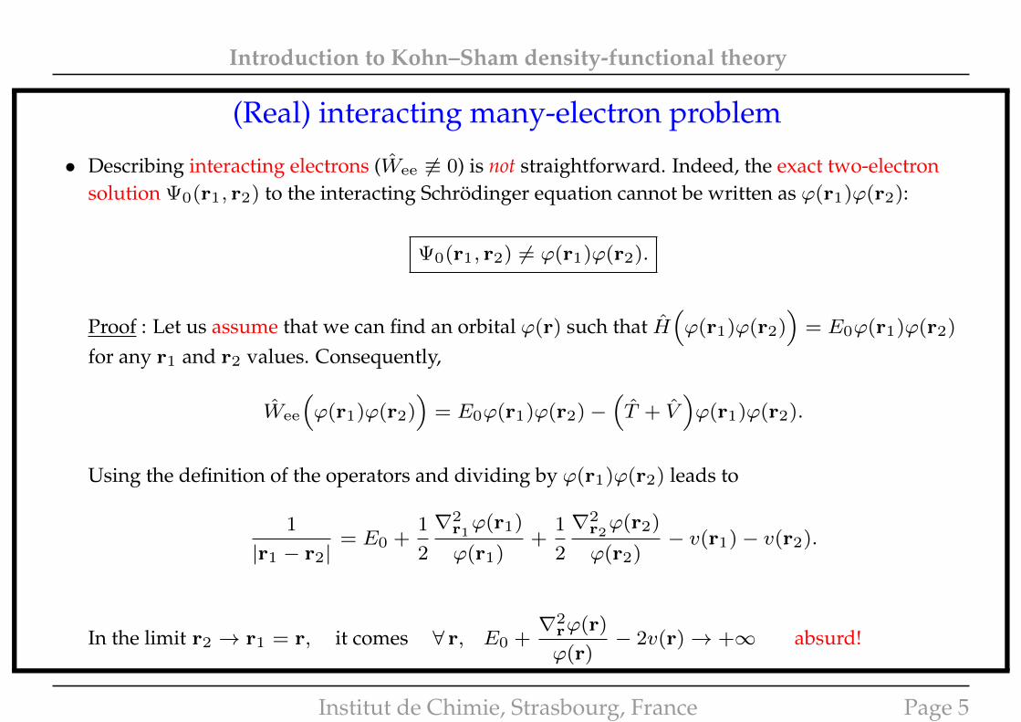
(Real) interacting many-electron problem
• Describing interacting electrons (Wee 6≡ 0) is not straightforward. Indeed, the exact two-electronsolution Ψ0(r1, r2) to the interacting Schrödinger equation cannot be written as ϕ(r1)ϕ(r2):
Ψ0(r1, r2) 6= ϕ(r1)ϕ(r2).
Proof : Let us assume that we can find an orbital ϕ(r) such that H(ϕ(r1)ϕ(r2)
)= E0ϕ(r1)ϕ(r2)
for any r1 and r2 values. Consequently,
Wee
(ϕ(r1)ϕ(r2)
)= E0ϕ(r1)ϕ(r2)−
(T + V
)ϕ(r1)ϕ(r2).
Using the definition of the operators and dividing by ϕ(r1)ϕ(r2) leads to
1
|r1 − r2|= E0 +
1
2
∇2r1ϕ(r1)
ϕ(r1)+
1
2
∇2r2ϕ(r2)
ϕ(r2)− v(r1)− v(r2).
In the limit r2 → r1 = r, it comes ∀ r, E0 +∇2
rϕ(r)
ϕ(r)− 2v(r)→ +∞ absurd!
Institut de Chimie, Strasbourg, France Page 5
Introduction to Kohn–Sham density-functional theory
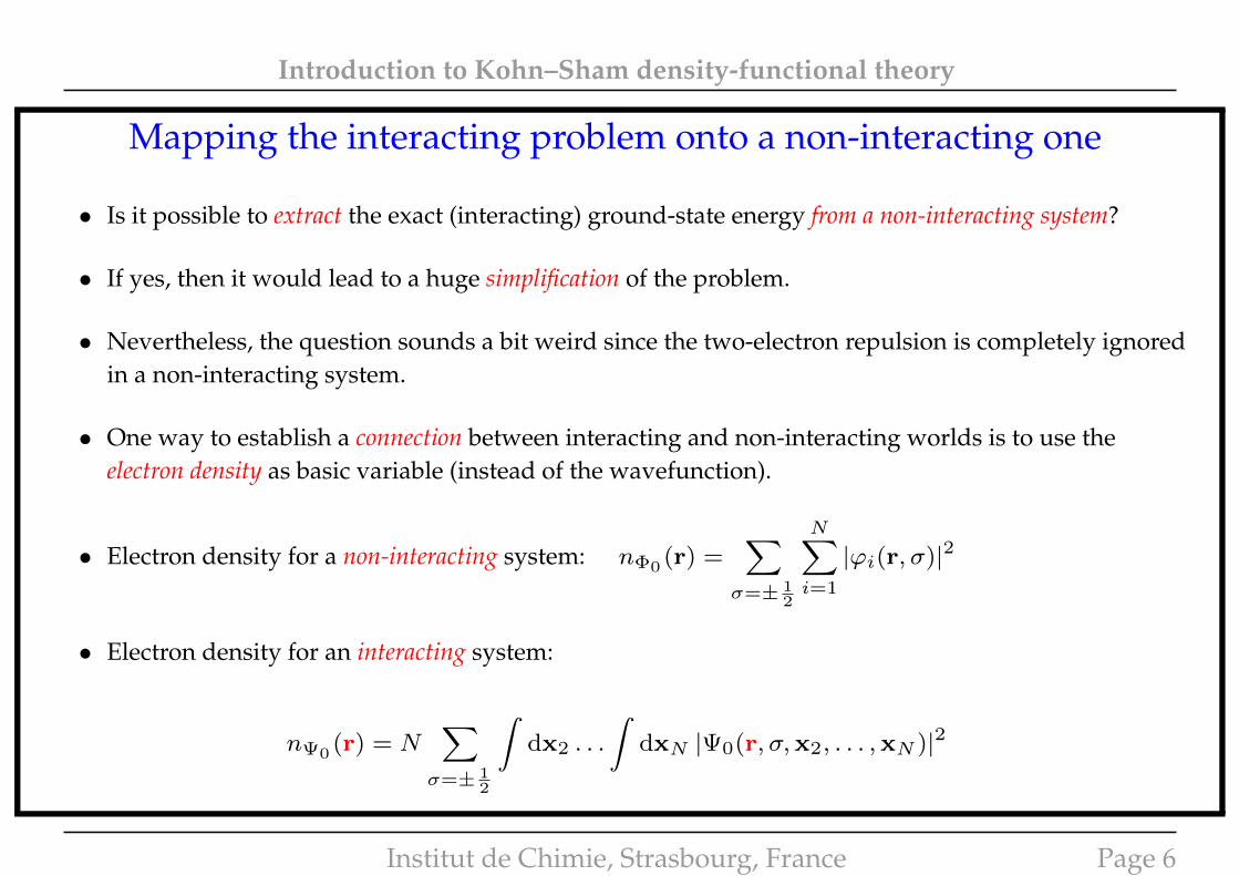
Mapping the interacting problem onto a non-interacting one
• Is it possible to extract the exact (interacting) ground-state energy from a non-interacting system?
• If yes, then it would lead to a huge simplification of the problem.
• Nevertheless, the question sounds a bit weird since the two-electron repulsion is completely ignoredin a non-interacting system.
• One way to establish a connection between interacting and non-interacting worlds is to use theelectron density as basic variable (instead of the wavefunction).
• Electron density for a non-interacting system: nΦ0(r) =
∑σ=± 1
2
N∑i=1
|ϕi(r, σ)|2
• Electron density for an interacting system:
nΨ0(r) = N
∑σ=± 1
2
∫dx2 . . .
∫dxN |Ψ0(r, σ,x2, . . . ,xN )|2
Institut de Chimie, Strasbourg, France Page 6
Introduction to Kohn–Sham density-functional theory
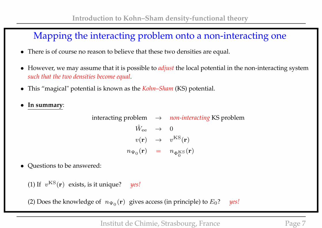
Mapping the interacting problem onto a non-interacting one
• There is of course no reason to believe that these two densities are equal.
• However, we may assume that it is possible to adjust the local potential in the non-interacting systemsuch that the two densities become equal.
• This “magical" potential is known as the Kohn–Sham (KS) potential.
• In summary:
interacting problem → non-interacting KS problem
Wee → 0
v(r) → vKS(r)
nΨ0 (r) = nΦKS0
(r)
• Questions to be answered:
(1) If vKS(r) exists, is it unique? yes!
(2) Does the knowledge of nΨ0(r) gives access (in principle) to E0? yes!
Institut de Chimie, Strasbourg, France Page 7
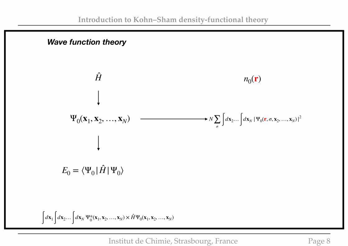
Introduction to Kohn–Sham density-functional theory
E0 = ⟨Ψ0 | H |Ψ0⟩
n0(r)
Ψ0(x1, x2, …, xN) N∑σ
∫ dx2…∫ dxN |Ψ0(r, σ, x2, …, xN) |2
=
∫ dx1 ∫ dx2…∫ dxN Ψ*0 (x1, x2, …, xN) × HΨ0(x1, x2, …, xN)
=
H
Wave function theory
Institut de Chimie, Strasbourg, France Page 8
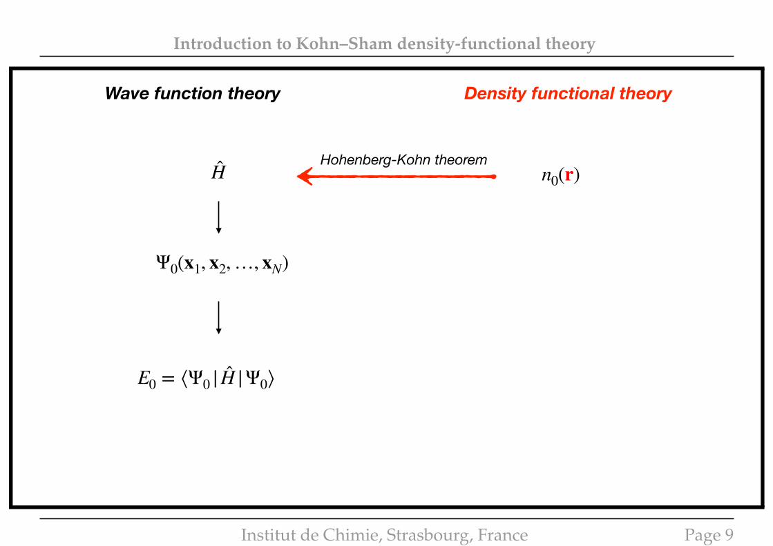
Introduction to Kohn–Sham density-functional theory
E0 = ⟨Ψ0 | H |Ψ0⟩
n0(r)
Ψ0(x1, x2, …, xN)
H
Wave function theory Density functional theory
Hohenberg-Kohn theorem
Institut de Chimie, Strasbourg, France Page 9
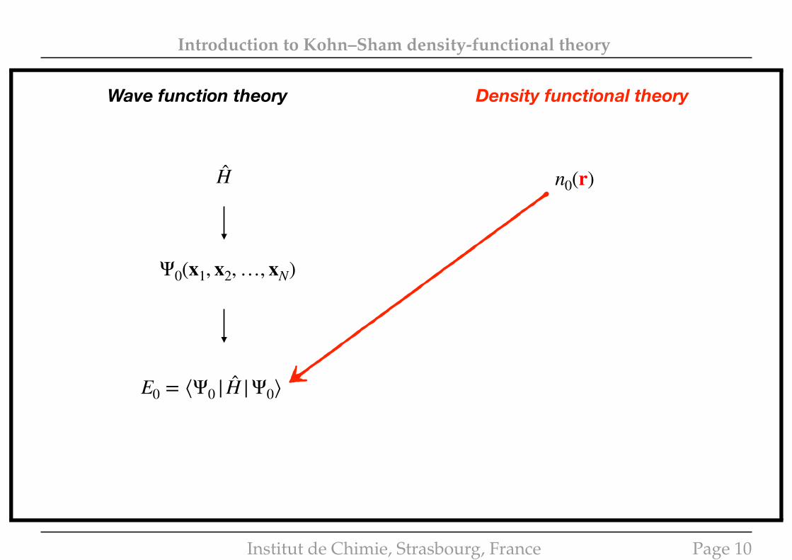
Introduction to Kohn–Sham density-functional theory
E0 = ⟨Ψ0 | H |Ψ0⟩
n0(r)
Ψ0(x1, x2, …, xN)
H
Wave function theory Density functional theory
Institut de Chimie, Strasbourg, France Page 10
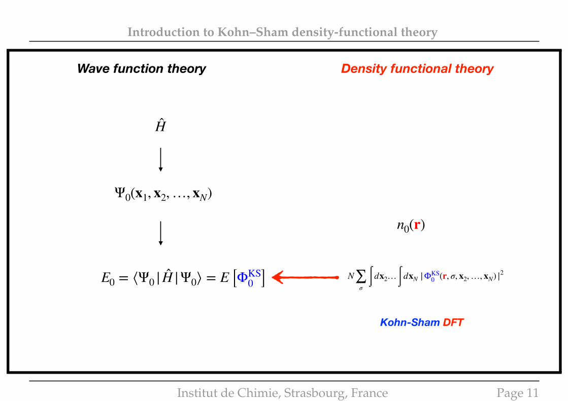
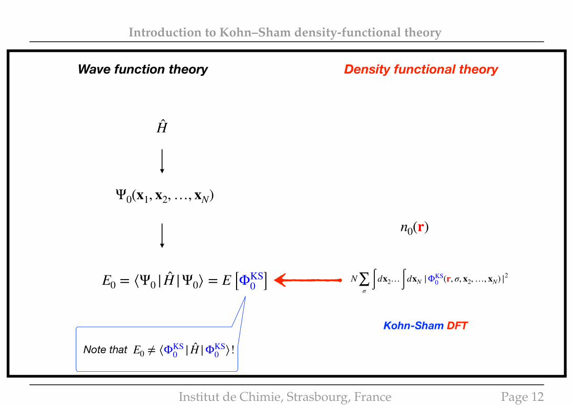
Introduction to Kohn–Sham density-functional theory
E0 = ⟨Ψ0 | H |Ψ0⟩ = E [ΦKS0 ]
n0(r)Ψ0(x1, x2, …, xN)
H
Wave function theory Density functional theory
N∑σ
∫ dx2…∫ dxN |ΦKS0 (r, σ, x2, …, xN) |2
=
Kohn-Sham DFT
Institut de Chimie, Strasbourg, France Page 11
Introduction to Kohn–Sham density-functional theory
E0 = ⟨Ψ0 | H |Ψ0⟩ = E [ΦKS0 ]
n0(r)Ψ0(x1, x2, …, xN)
H
Wave function theory Density functional theory
N∑σ
∫ dx2…∫ dxN |ΦKS0 (r, σ, x2, …, xN) |2
=
Kohn-Sham DFT
Note that E0 ≠ ⟨ΦKS0 | H |ΦKS0 ⟩!
Institut de Chimie, Strasbourg, France Page 12
Introduction to Kohn–Sham density-functional theory
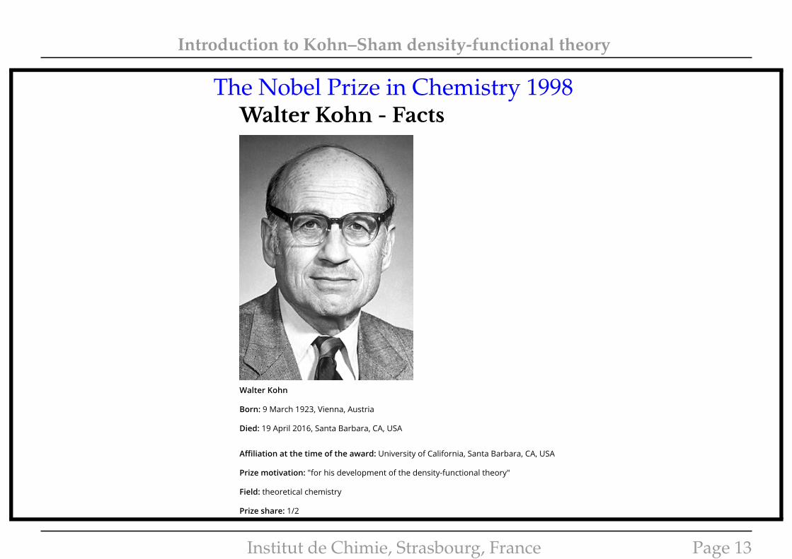
The Nobel Prize in Chemistry 1998
This website uses cookies to improve user experience. By using our website you consent to all cookies inaccordance with our Cookie Policy.
I UNDERSTAND
Share this: 6
The Nobel Prize in Chemistry 1998
Walter Kohn, John Pople
Walter Kohn - Facts
WorkThe structures of molecules and the way they react with one another depends on the movement of electrons and their
distribution in space, which is determined by the laws of quantum mechanics. However, quantum mechanics requires
very complicated calculations for complex systems such as molecules. In 1964 Walter Kohn laid the foundation for a
theory that stated it was not necessary to account for every electron's movement. Instead, one could look at the
average density of electrons in the space. This presented new opportunities for calculations involving chemical
structures and reactions.
Walter Kohn
Born: 9 March 1923, Vienna, Austria
Died: 19 April 2016, Santa Barbara, CA, USA
Affiliation at the time of the award: University of California, Santa Barbara, CA, USA
Prize motivation: "for his development of the density-functional theory"
Field: theoretical chemistry
Prize share: 1/2
Walter Kohn - Facts https://www.nobelprize.org/nobel_prizes/chemistry/laureates/...
1 of 2 23/02/2017, 10:24
Institut de Chimie, Strasbourg, France Page 13
Introduction to Kohn–Sham density-functional theory
Three things to remember before we start ...
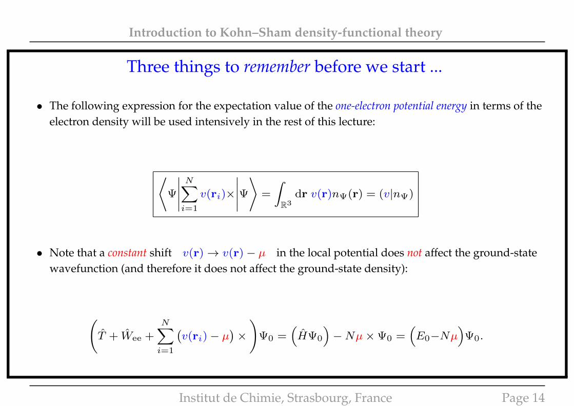
• The following expression for the expectation value of the one-electron potential energy in terms of theelectron density will be used intensively in the rest of this lecture:
⟨Ψ
∣∣∣∣∣N∑i=1
v(ri)×
∣∣∣∣∣Ψ⟩
=
∫R3
dr v(r)nΨ(r) = (v|nΨ)
• Note that a constant shift v(r)→ v(r)− µ in the local potential does not affect the ground-statewavefunction (and therefore it does not affect the ground-state density):
(T + Wee +
N∑i=1
(v(ri)− µ
)×)
Ψ0 =(HΨ0
)−Nµ×Ψ0 =
(E0−Nµ
)Ψ0.
Institut de Chimie, Strasbourg, France Page 14
Introduction to Kohn–Sham density-functional theory
Three things to remember before we start ...
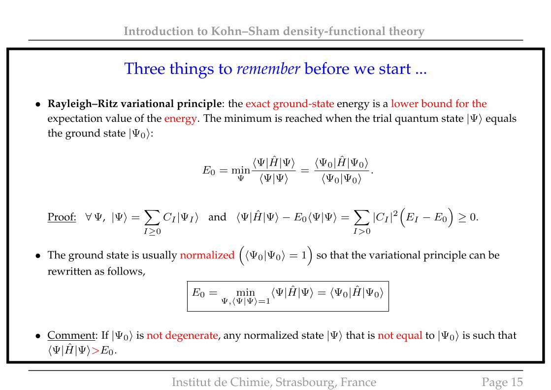
• Rayleigh–Ritz variational principle: the exact ground-state energy is a lower bound for theexpectation value of the energy. The minimum is reached when the trial quantum state |Ψ〉 equalsthe ground state |Ψ0〉:
E0 = minΨ
〈Ψ|H|Ψ〉〈Ψ|Ψ〉
=〈Ψ0|H|Ψ0〉〈Ψ0|Ψ0〉
.
Proof: ∀Ψ, |Ψ〉 =∑I≥0
CI |ΨI〉 and 〈Ψ|H|Ψ〉 − E0〈Ψ|Ψ〉 =∑I>0
|CI |2(EI − E0
)≥ 0.
• The ground state is usually normalized(〈Ψ0|Ψ0〉 = 1
)so that the variational principle can be
rewritten as follows,
E0 = minΨ,〈Ψ|Ψ〉=1
〈Ψ|H|Ψ〉 = 〈Ψ0|H|Ψ0〉
• Comment: If |Ψ0〉 is not degenerate, any normalized state |Ψ〉 that is not equal to |Ψ0〉 is such that〈Ψ|H|Ψ〉>E0.
Institut de Chimie, Strasbourg, France Page 15
Introduction to Kohn–Sham density-functional theory
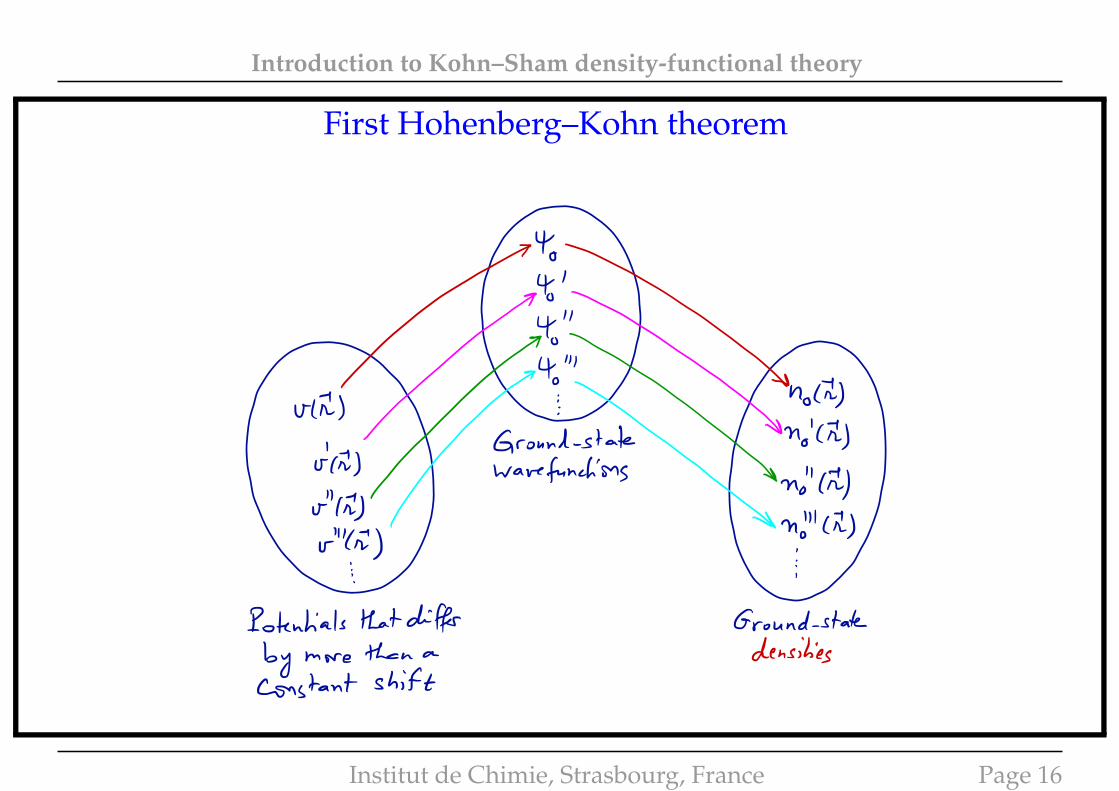
First Hohenberg–Kohn theorem
4
¥
.run ,i "
jet ) wavefunctionsno
"C I )
v"
cryno "ci ,r' " Ci ) .
'
i.
i
Potentials that differ Ground -state
by more than a densitiesConstant shift
Institut de Chimie, Strasbourg, France Page 16
Introduction to Kohn–Sham density-functional theory
First Hohenberg–Kohn theorem
• Note that v → Ψ0 → E0
→ n0 = nΨ0
• HK1: Hohenberg and Kohn∗ have shown that, in fact, the ground-state electron density fullydetermines (up to a constant) the local potential v. Therefore
n0 → v → Ψ0 → E0
• In other words, the ground-state energy is a functional of the ground-state density: E0 = E[n0].
Proof (part 1):
Let us consider two potentials v and v′ that differ by more than a constant, which means that v(r)− v′(r)
varies with r. In the following, we denote Ψ0 and Ψ′0 the associated ground-state wavefunctions withenergies E0 and E′0, respectively.
∗P. Hohenberg and W. Kohn, Phys. Rev. 136, B864 (1964).
Institut de Chimie, Strasbourg, France Page 17
Introduction to Kohn–Sham density-functional theory
First Hohenberg–Kohn theorem
If Ψ0 = Ψ′0 then
N∑i=1
(v(ri)− v′(ri)
)×Ψ0 =
N∑i=1
v(ri)×Ψ0 − v′(ri)×Ψ′0
=
(T + Wee +
N∑i=1
v(ri)×)
Ψ0 −(T + Wee +
N∑i=1
v′(ri)×)
Ψ′0
= E0Ψ0 − E′0Ψ′0
=(E0 − E′0
)×Ψ0
so that, in the particular case r1 = r2 = . . . = rN = r, we obtain
v(r)− v′(r) =(E0 − E′0
)/N −→ constant (absurd !)
Therefore Ψ0 and Ψ′0 cannot be equal.
Institut de Chimie, Strasbourg, France Page 18
Introduction to Kohn–Sham density-functional theory
First Hohenberg–Kohn theorem
Proof (part 2): Let us now assume that Ψ0 and Ψ′0 have the same electron density n0.
According to the Rayleigh–Ritz variational principle
E0 <
⟨Ψ′0
∣∣∣∣∣T + Wee +
N∑i=1
v(ri)×
∣∣∣∣∣Ψ′0⟩
︸ ︷︷ ︸ and E′0 <
⟨Ψ0
∣∣∣∣∣T + Wee +
N∑i=1
v′(ri)×
∣∣∣∣∣Ψ0
⟩︸ ︷︷ ︸
E′0 + (v − v′|n0) E0 − (v − v′|n0)
thus leading to
0 < E0 − E′0 − (v − v′|n0) < 0 absurd !
∗P. Hohenberg and W. Kohn, Phys. Rev. 136, B864 (1964).
Institut de Chimie, Strasbourg, France Page 19
Introduction to Kohn–Sham density-functional theory
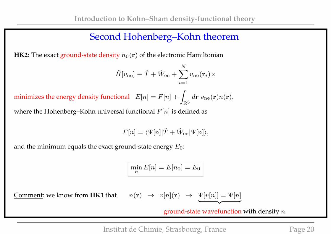
Second Hohenberg–Kohn theorem
HK2: The exact ground-state density n0(r) of the electronic Hamiltonian
H[vne] ≡ T + Wee +N∑i=1
vne(ri)×
minimizes the energy density functional E[n] = F [n] +
∫R3dr vne(r)n(r),
where the Hohenberg–Kohn universal functional F [n] is defined as
F [n] = 〈Ψ[n]|T + Wee|Ψ[n]〉,
and the minimum equals the exact ground-state energy E0:
minnE[n] = E[n0] = E0
Comment: we know from HK1 that n(r) → v[n](r) → Ψ[v[n]] = Ψ[n]︸ ︷︷ ︸ground-state wavefunction with density n.
Institut de Chimie, Strasbourg, France Page 20
Introduction to Kohn–Sham density-functional theory
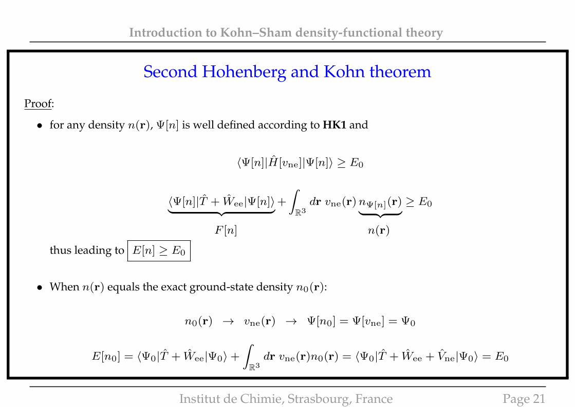
Second Hohenberg and Kohn theorem
Proof:
• for any density n(r), Ψ[n] is well defined according to HK1 and
〈Ψ[n]|H[vne]|Ψ[n]〉 ≥ E0
〈Ψ[n]|T + Wee|Ψ[n]〉︸ ︷︷ ︸+
∫R3dr vne(r)nΨ[n](r)︸ ︷︷ ︸ ≥ E0
F [n] n(r)
thus leading to E[n] ≥ E0
• When n(r) equals the exact ground-state density n0(r):
n0(r) → vne(r) → Ψ[n0] = Ψ[vne] = Ψ0
E[n0] = 〈Ψ0|T + Wee|Ψ0〉+
∫R3dr vne(r)n0(r) = 〈Ψ0|T + Wee + Vne|Ψ0〉 = E0
Institut de Chimie, Strasbourg, France Page 21
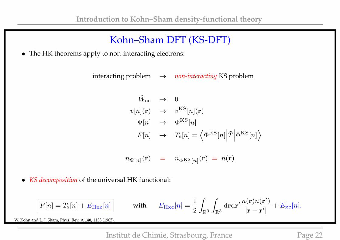
Introduction to Kohn–Sham density-functional theory
Kohn–Sham DFT (KS-DFT)• The HK theorems apply to non-interacting electrons:
interacting problem → non-interacting KS problem
Wee → 0
v[n](r) → vKS[n](r)
Ψ[n] → ΦKS[n]
F [n] → Ts[n] =⟨
ΦKS[n]∣∣∣T ∣∣∣ΦKS[n]
⟩nΨ[n](r) = nΦKS[n](r) = n(r)
• KS decomposition of the universal HK functional:
F [n] = Ts[n] + EHxc[n] with EHxc[n] =1
2
∫R3
∫R3
drdr′n(r)n(r′)
|r− r′|+ Exc[n].
W. Kohn and L. J. Sham, Phys. Rev. A 140, 1133 (1965).
Institut de Chimie, Strasbourg, France Page 22
Introduction to Kohn–Sham density-functional theory
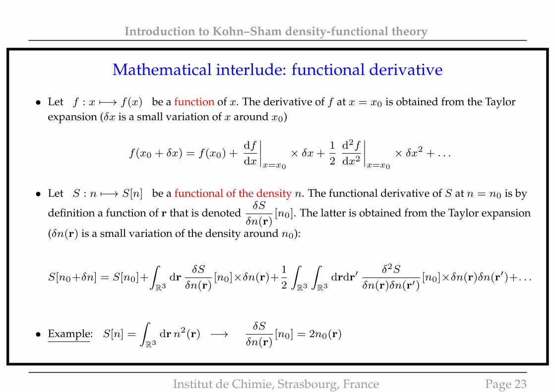
Mathematical interlude: functional derivative
• Let f : x 7−→ f(x) be a function of x. The derivative of f at x = x0 is obtained from the Taylorexpansion (δx is a small variation of x around x0)
f(x0 + δx) = f(x0) +df
dx
∣∣∣∣x=x0
× δx+1
2
d2f
dx2
∣∣∣∣x=x0
× δx2 + . . .
• Let S : n 7−→ S[n] be a functional of the density n. The functional derivative of S at n = n0 is by
definition a function of r that is denotedδS
δn(r)[n0]. The latter is obtained from the Taylor expansion
(δn(r) is a small variation of the density around n0):
S[n0+δn] = S[n0]+
∫R3
drδS
δn(r)[n0]×δn(r)+
1
2
∫R3
∫R3
drdr′δ2S
δn(r)δn(r′)[n0]×δn(r)δn(r′)+. . .
• Example: S[n] =
∫R3
drn2(r) −→δS
δn(r)[n0] = 2n0(r)
Institut de Chimie, Strasbourg, France Page 23
Introduction to Kohn–Sham density-functional theory
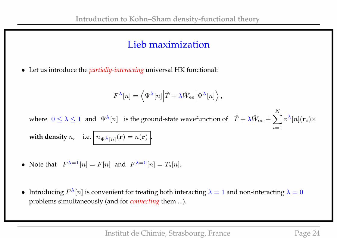
Lieb maximization
• Let us introduce the partially-interacting universal HK functional:
Fλ[n] =⟨
Ψλ[n]∣∣∣T + λWee
∣∣∣Ψλ[n]⟩,
where 0 ≤ λ ≤ 1 and Ψλ[n] is the ground-state wavefunction of T + λWee +N∑i=1
vλ[n](ri)×
with density n, i.e. nΨλ[n](r) = n(r) .
• Note that Fλ=1[n] = F [n] and Fλ=0[n] = Ts[n].
• Introducing Fλ[n] is convenient for treating both interacting λ = 1 and non-interacting λ = 0
problems simultaneously (and for connecting them ...).
Institut de Chimie, Strasbourg, France Page 24
Introduction to Kohn–Sham density-functional theory
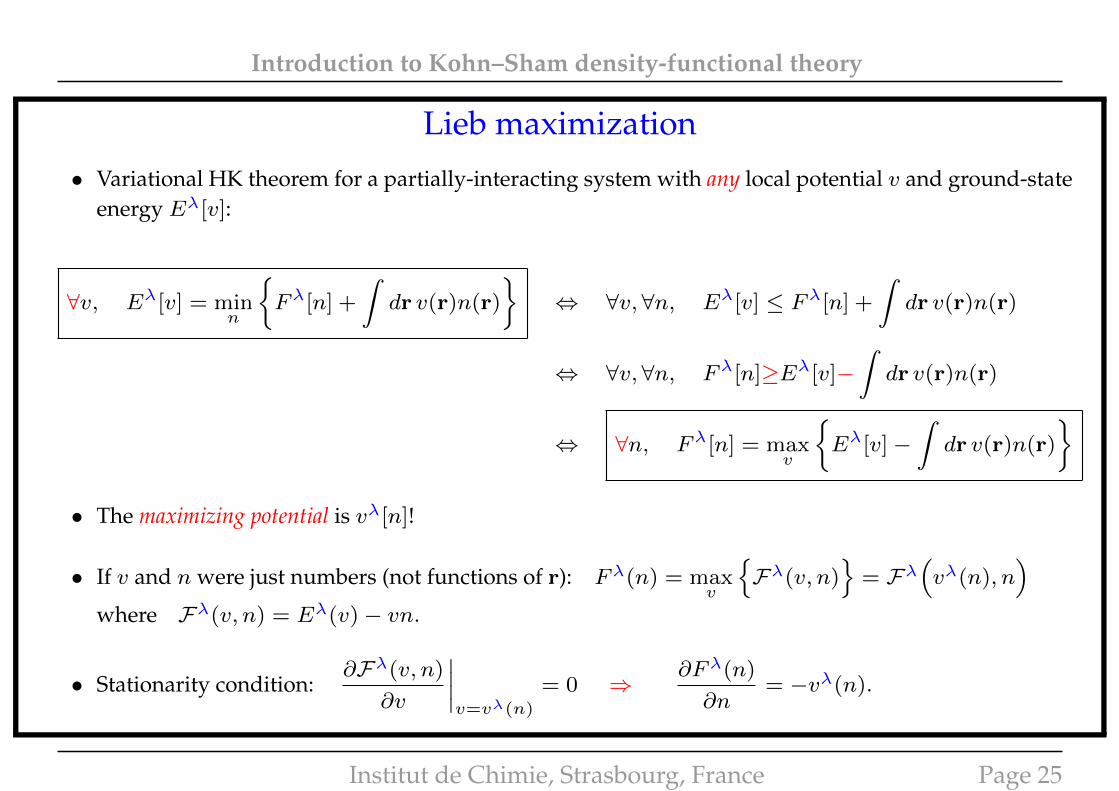
Lieb maximization
• Variational HK theorem for a partially-interacting system with any local potential v and ground-stateenergy Eλ[v]:
∀v, Eλ[v] = minn
{Fλ[n] +
∫dr v(r)n(r)
}⇔ ∀v,∀n, Eλ[v] ≤ Fλ[n] +
∫dr v(r)n(r)
⇔ ∀v,∀n, Fλ[n]≥Eλ[v]−∫dr v(r)n(r)
⇔ ∀n, Fλ[n] = maxv
{Eλ[v]−
∫dr v(r)n(r)
}
• The maximizing potential is vλ[n]!
• If v and n were just numbers (not functions of r): Fλ(n) = maxv
{Fλ(v, n)
}= Fλ
(vλ(n), n
)where Fλ(v, n) = Eλ(v)− vn.
• Stationarity condition:∂Fλ(v, n)
∂v
∣∣∣∣v=vλ(n)
= 0 ⇒∂Fλ(n)
∂n= −vλ(n).
Institut de Chimie, Strasbourg, France Page 25
Introduction to Kohn–Sham density-functional theory
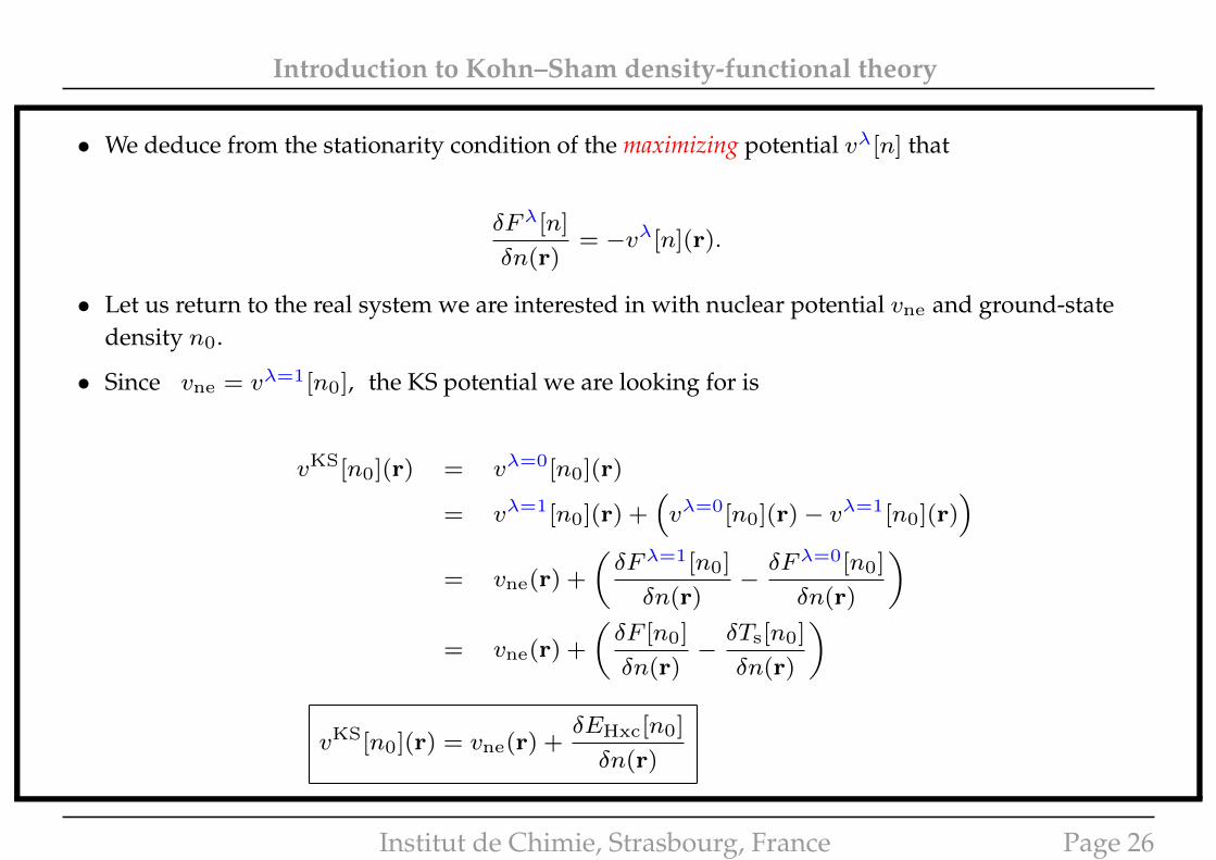
• We deduce from the stationarity condition of the maximizing potential vλ[n] that
δFλ[n]
δn(r)= −vλ[n](r).
• Let us return to the real system we are interested in with nuclear potential vne and ground-statedensity n0.
• Since vne = vλ=1[n0], the KS potential we are looking for is
vKS[n0](r) = vλ=0[n0](r)
= vλ=1[n0](r) +(vλ=0[n0](r)− vλ=1[n0](r)
)= vne(r) +
(δFλ=1[n0]
δn(r)−δFλ=0[n0]
δn(r)
)= vne(r) +
(δF [n0]
δn(r)−δTs[n0]
δn(r)
)
vKS[n0](r) = vne(r) +δEHxc[n0]
δn(r)
Institut de Chimie, Strasbourg, France Page 26
Introduction to Kohn–Sham density-functional theory
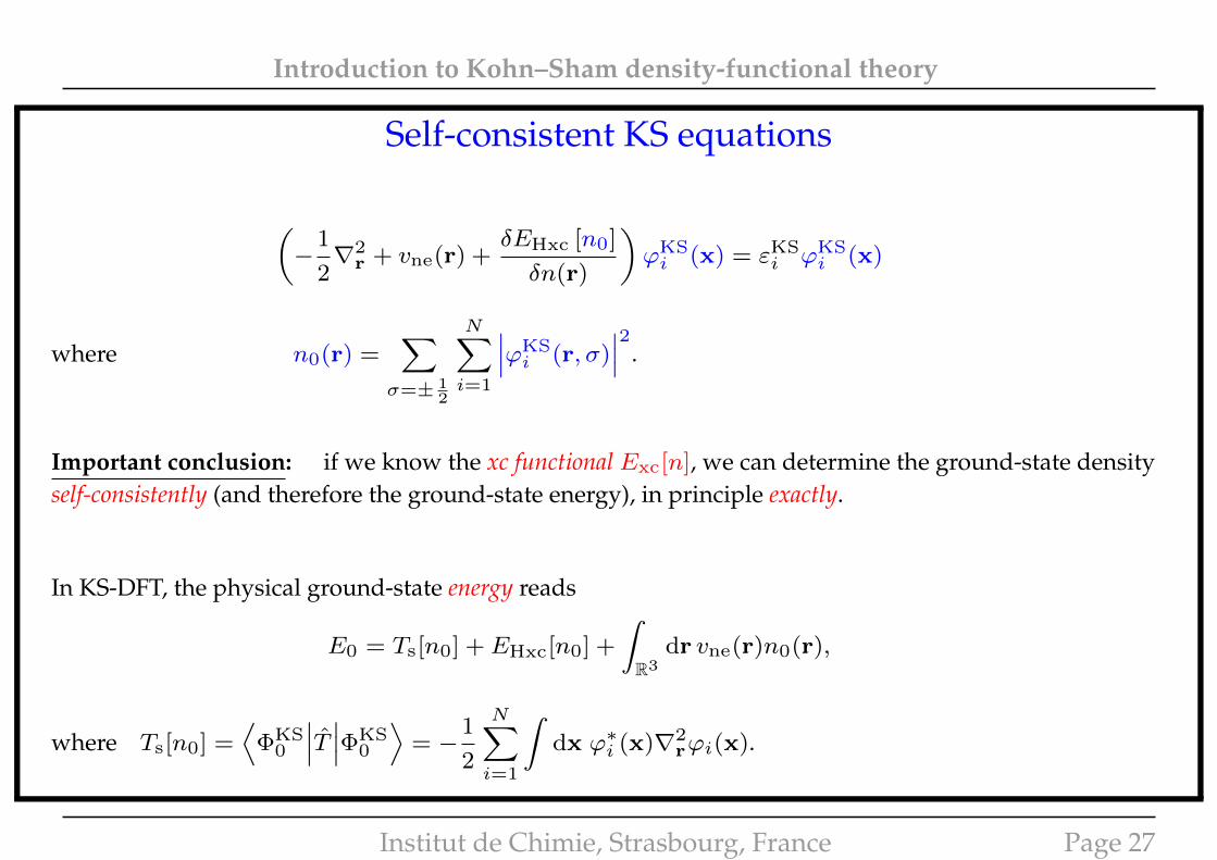
Self-consistent KS equations
(−
1
2∇2
r + vne(r) +δEHxc [n0]
δn(r)
)ϕKSi (x) = εKS
i ϕKSi (x)
where n0(r) =∑σ=± 1
2
N∑i=1
∣∣∣ϕKSi (r, σ)
∣∣∣2.
Important conclusion: if we know the xc functional Exc[n], we can determine the ground-state densityself-consistently (and therefore the ground-state energy), in principle exactly.
In KS-DFT, the physical ground-state energy reads
E0 = Ts[n0] + EHxc[n0] +
∫R3
dr vne(r)n0(r),
where Ts[n0] =⟨
ΦKS0
∣∣∣T ∣∣∣ΦKS0
⟩= −
1
2
N∑i=1
∫dx ϕ∗i (x)∇2
rϕi(x).
Institut de Chimie, Strasbourg, France Page 27
Recommended


![Constrained DFT (CDFT) in CP2K2018_user_meeting:cp2...• Approximate electronic coupling withCDFT Kohn-Sham determinants after orthogonalization [5] tij≈ ´CDFT i * KS ´CDFT j](https://img.pdfslide.us/doc/110x75/5f714beffac757466d5f289b/constrained-dft-cdft-in-cp2k-2018usermeetingcp2-a-approximate-electronic.jpg)