Practical course using the software
—————Introduction to genetic data analysis in
Thibaut Jombart
—————
Abstract
This practical course is meant as a short introduction to genetic dataanalysis using [10]. After describing the main types of data, we illus-trate how to perform some basic population genetics analyses, and then gothrough constructing trees from genetic distances and performing standardmultivariate analyses. The practical uses mostly the packages adegenet [6],ape [9] and ade4 [1, 3, 2], but others like genetics [11] and hierfstat [5] arealso required.
1
Contents
1 Let’s start 31.1 Loading the packages . . . . . . . . . . . . . . . . . . . . . . . 31.2 How to get information? . . . . . . . . . . . . . . . . . . . . . 3
2 Handling the data 52.1 Data formats . . . . . . . . . . . . . . . . . . . . . . . . . . . 52.2 Importing / exporting data . . . . . . . . . . . . . . . . . . . 72.3 Manipulating data . . . . . . . . . . . . . . . . . . . . . . . . 8
3 Basic population genetics 9
4 Making trees 114.1 Hierarchical clustering . . . . . . . . . . . . . . . . . . . . . . 114.2 ape and phylogenies . . . . . . . . . . . . . . . . . . . . . . . 13
5 Multivariate Analysis 155.1 ade4 . . . . . . . . . . . . . . . . . . . . . . . . . . . . . . . . 155.2 Principal Component Analysis (PCA) . . . . . . . . . . . . . 165.3 Principal Coordinates Analysis (PCoA) . . . . . . . . . . . . 19
2
1 Let’s start
1.1 Loading the packages
Before going further, we shall make sure that all we need is installed on thecomputer. Launch , and make sure that the version being used is at least2.12.0 by typing:
> R.version.string
[1] "R version 2.12.0 (2010-10-15)"
The next thing to do is check that relevant packages are installed. To loadan installed package, use the library instruction; for instance:
> library(adegenet)
loads adegenet if it is installed (and issues an error otherwise). To get theversion of a package, use:
> packageDescription("adegenet", fields = "Version")
[1] "1.2-9"
adegenet version should read 1.2-8 or greater.In case a package would not be installed, you can install it using in-
stall.packages. To install all the required dependencies, specify dep=TRUE.For instance, the following instruction should install adegenet with all its de-pendencies (it can take up to a few minutes, so don’t run it unless adegenetis not installed):
> install.packages("adegenet", dep = TRUE)
Using the previous instructions, load (and install if required) the pack-ages adegenet, ade4, ape, genetics, and hierfstat.
1.2 How to get information?
There are several ways of getting information about R in general, or aboutadegenet in particular. The function help.search is used to look for helpon a given topic. For instance:
> help.search("Hardy-Weinberg")
replies that there is a function HWE.test.genind in the adegenet package,other similar functions in genetics and pegas. To get help for a given func-tion, use ?foo where ‘foo’ is the function of interest. For instance (quotescan be removed):
> `?`(spca)
3
will open the manpage of the spatial principal component analysis [7]. Atthe end of a manpage, an ‘example’ section often shows how to use a func-tion. This can be copied and pasted to the console, or directly executedfrom the console using example. For further questions concerning R, thefunction RSiteSearch is a powerful tool to make an online research usingkeywords in R’s archives (mailing lists and manpages).
adegenet has a few extra documentation sources. Information can befound from the website (http://adegenet.r-forge.r-project.org/), inthe ‘documents’ section, including two tutorials, a manual which includesall manpages of the package, and a dedicated mailing list with searchablearchives. To open the website from , use:
> adegenetWeb()
The same can be done for tutorials, using adegenetTutorial (see manpageto choose the tutorial to open).
You will also find a listing of the main functions of the package typing:
> `?`(adegenet)
Note that you can also browse help pages as html pages, using:
> help.start()
To go to the adegenet page, click ‘packages’, ‘adegenet’, and ‘adegenet-package’.
Lastly, several mailing lists are available to find different kinds of infor-mation on R; to name a few:
R-help (https://stat.ethz.ch/mailman/listinfo/r-help): general ques-tions about R
R-sig-genetics (https://stat.ethz.ch/mailman/listinfo/r-sig-genetics):genetics in R
adegenet forum (https://lists.r-forge.r-project.org/cgi-bin/mailman/listinfo/adegenet-forum): adegenet and multivariate analysis ofgenetic markers
4
2 Handling the data
2.1 Data formats
Two principal types of genetic data can be handled in R. The first one is(preferably aligned) DNA sequences, and the second one is genetic markers.
DNA sequences can be used to calibrate models of evolution and computegenetic distances, which can in turn be used for phylogenetic reconstructionor in multivariate analyses. In , DNA sequences are best handled asDNAbin objects, in the ape package. See ?DNAbin for more details about thisclass. After loading ape, we load the dataset woodmouse:
> library(ape)> data(woodmouse)> woodmouse
15 DNA sequences in binary format stored in a matrix.
All sequences of same length: 965
Labels: No305 No304 No306 No0906S No0908S No0909S ...
Base composition:a c g t
0.307 0.261 0.126 0.306
Use str, unclass and attributes to explore the content of the DNAbin
object. Convert the dataset to a matrix of characters using as.character.What is the size of this new object (use object.size)? Compare it to theoriginal DNAbin object. Why is this class optimal for handling DNA se-quences?
Genetic markers are features of DNA sequences that vary between indi-viduals. There is not a single type of genetic marker: some are codominant(all alleles are visible), some are dominant (some alleles hide the presence ofothers); some have many alleles (like microsatellites), and others are most of-ten binary (like SNPs). In general, codominant (more informative) markersare the rule, and dominant markers become more and more rare.
Both types of markers can be handled in using the class genind
implemented in adegenet. This class uses the S4 system of class definitionand methods, with which users are generally not familiar. Load thedataset nancycats:
> library(adegenet)> data(nancycats)> nancycats
######################## Genind object ########################
- genotypes of individuals -
5
S4 class: genind@call: genind(tab = truenames(nancycats)$tab, pop = truenames(nancycats)$pop)
@tab: 237 x 108 matrix of genotypes
@ind.names: vector of 237 individual [email protected]: vector of 9 locus [email protected]: number of alleles per [email protected]: locus factor for the 108 columns of @[email protected]: list of 9 components yielding allele names for each locus@ploidy: 2@type: codom
Optionnal contents:@pop: factor giving the population of each [email protected]: factor giving the population of each individual
@other: a list containing: xy
Usually, the slots of S4 objects can be accessed by ’@’, which replaces the$ operator used in S3 classes (e.g. in lists). For genind objects, both canbe used. Documentation of the class can be accessed by typing ?’genind-
class’. Using names and @ (or $), browse the content of nancycats; whatinformation is contained in this object?
A more simple dataset can be used to understand how information iscoded. Here, we create a simple dataset with two diploid individuals (inrows), and two markers (columns).
> dat <- data.frame(locus1 = c("A/T", "T/T"), locus2 = c("G/G",+ "C/G"))> dat
locus1 locus21 A/T G/G2 T/T C/G
> x <- df2genind(dat, sep = "/")> x
######################## Genind object ########################
- genotypes of individuals -
S4 class: genind@call: df2genind(X = dat, sep = "/")
@tab: 2 x 4 matrix of genotypes
@ind.names: vector of 2 individual [email protected]: vector of 2 locus [email protected]: number of alleles per [email protected]: locus factor for the 4 columns of @[email protected]: list of 2 components yielding allele names for each locus@ploidy: 2@type: codom
Optionnal contents:@pop: - empty -
6
@pop.names: - empty -
@other: - empty -
Look at the @tab component of the genind object. To extract this tablewith original labels, use truenames. How is information stored? Does theEuclidean distance between the rows of this matrix make some biologicalsense? This is a canonical way of storing information for any dominantmarkers, irrespective of the degree of ploidy.
It sometimes happens that analyses are performed at a population level,rather than at an individual level. In such cases, genpop objects are used.These objects contain allele numbers per populations rather than relativefrequencies, but are otherwise similar to genind objects. genpop can beobtained from genind objects using genind2genpop. Use this function tocompute allele counts for the cat colonies of Nancy (data nancycats), andcompare the the structure of the obtained object to the genind object.
2.2 Importing / exporting data
DNA sequences with usual formats are read using read.dna from the apepackage.
Genetic markers come in a wider variety of formats. import2genind
can be used to import some of the most frequent, and less twisted formats.However, it is also possible to convert data from a data.frame to a genindusing df2genind. Using the example above, create a data.frame with twotetraploid (i.e. 4 alleles) individuals and two loci. Note that alleles can begiven any name, and do not need to be letters. Then, used df2genind toconvert it to a genind object. Use truenames and genind2df to check thatthe data conversion has worked.
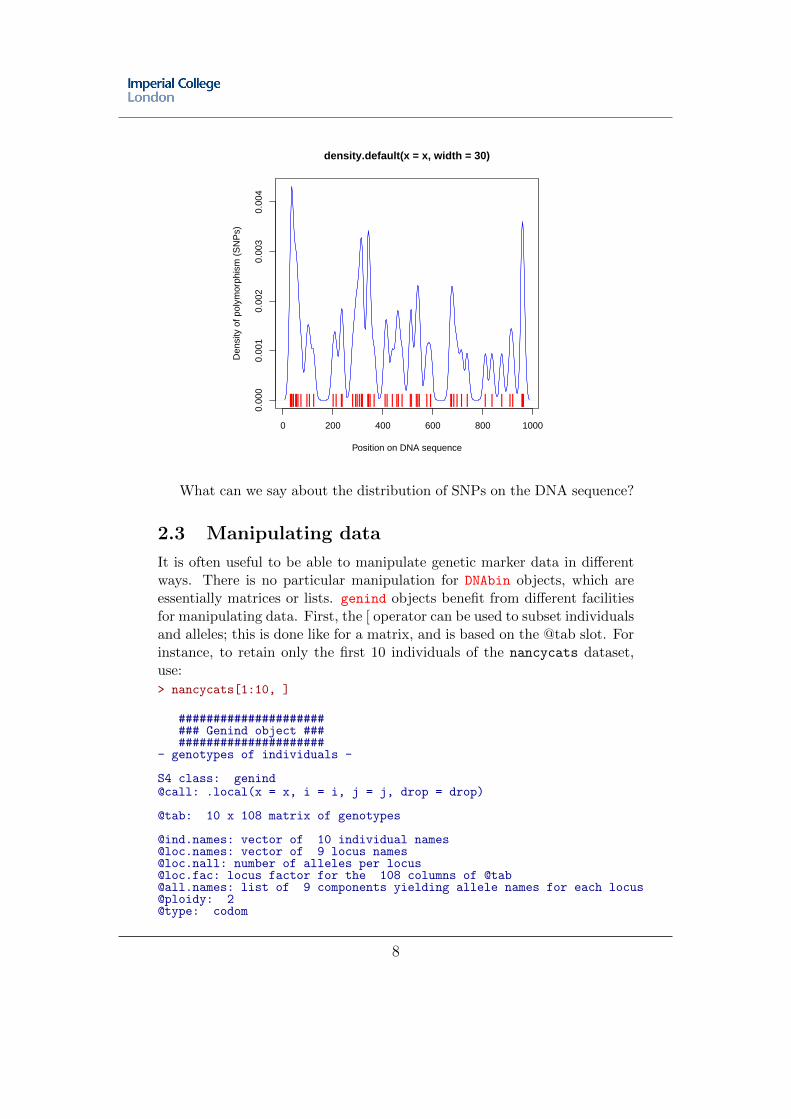
It also happens that genetic markers are derived from DNA sequences.In such a case, only sites that vary between individuals are retained; theseare called Single Nucleotide Polymorphism (SNPs). They can be extractedfrom DNAbin objects using DNAbin2genind. Use this function to extract thepolymorphic sites from the woodmouse dataset. The locus names correspondto the position of the polymorphic site. Use this information to plot thedistribution of polymorphism along the DNA sequence; you should arrive atsomething along the lines of (using density with a width of 30):
7
0 200 400 600 800 1000
0.00
00.
001
0.00
20.
003
0.00
4
density.default(x = x, width = 30)
Position on DNA sequence
Den
sity
of p
olym
orph
ism
(S
NP
s)
||||||||| ||| || || ||||||| ||||| || |||| || ||| || ||||| | | | | || ||||
What can we say about the distribution of SNPs on the DNA sequence?
2.3 Manipulating data
It is often useful to be able to manipulate genetic marker data in differentways. There is no particular manipulation for DNAbin objects, which areessentially matrices or lists. genind objects benefit from different facilitiesfor manipulating data. First, the [ operator can be used to subset individualsand alleles; this is done like for a matrix, and is based on the @tab slot. Forinstance, to retain only the first 10 individuals of the nancycats dataset,use:
> nancycats[1:10, ]
######################## Genind object ########################
- genotypes of individuals -
S4 class: genind@call: .local(x = x, i = i, j = j, drop = drop)
@tab: 10 x 108 matrix of genotypes
@ind.names: vector of 10 individual [email protected]: vector of 9 locus [email protected]: number of alleles per [email protected]: locus factor for the 108 columns of @[email protected]: list of 9 components yielding allele names for each locus@ploidy: 2@type: codom
8

Optionnal contents:@pop: factor giving the population of each [email protected]: factor giving the population of each individual
@other: a list containing: xy
Data can be split by population using seppop, and by locus using seploc.Indication of the population is obtained or set using pop. repool can beused to gather the genotypes stored in different genind objects into a singlegenind. Reading the documentation, interprete the following command line:
> temp <- seppop(nancycats)> x <- repool(lapply(temp, function(e) e[sample(1:nrow(e$tab),+ 5, replace = FALSE)]))
What does the produced object contain? How can this be useful whenanalysing genetic data?
3 Basic population genetics
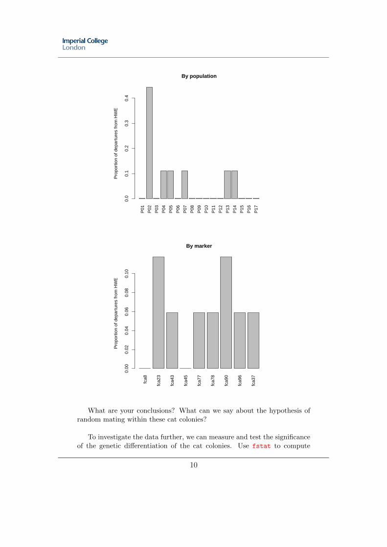
This section aims at introducing some basic population genetics tools. Thefirst one consists in testing random mating within groups by testing Hardy-Weinberg equilibirum (HWE). Using HWE.test.genind, test HWE in thecat colonies of the dataset nancycats. Since this corresponds to a lot of tests(1 per group and locus), as a first approximation, ask for returning only thep-values. Compute the number of significant departures from HWE (p.value< 0.001) per locus, and then per population (use apply), and representgraphically the results. You should arrive at (in less than 3 command lines):
9
P01
P02
P03
P04
P05
P06
P07
P08
P09
P10
P11
P12
P13
P14
P15
P16
P17
By population
Pro
port
ion
of d
epar
ture
s fr
om H
WE
0.0
0.1
0.2
0.3
0.4
fca8
fca2
3
fca4
3
fca4
5
fca7
7
fca7
8
fca9
0
fca9
6
fca3
7By marker
Pro
port
ion
of d
epar
ture
s fr
om H
WE
0.00
0.02
0.04
0.06
0.08
0.10
What are your conclusions? What can we say about the hypothesis ofrandom mating within these cat colonies?
To investigate the data further, we can measure and test the significanceof the genetic differentiation of the cat colonies. Use fstat to compute
10
the Fst of these populations. This is a measure of population differentia-tion, which can be roughly interpreted as the proportion of genetic varianceexplained by differences between groups. Values less than 0.05 are oftenconsidered as negligible.
Then, test the significance of the overall group differentiation usinggstat.randtest, and plot the results; are there differences between groups?
4 Making trees
Genetic data are often represented using trees. In this section, we won’ttackle phylogenetic reconstruction based on maximum likelihood or parsi-mony, which should be covered in a practical of its own. For this, see thewell-documented package phangorn. In the following, we illustrate brieflyhow to contruct tree representations of genetic distances.
4.1 Hierarchical clustering
Several algorithm of hierarchical clustering are implemented in the functionhclust. This function requires a distance matrix produced by the functiondist, or similar function (e.g. dist.dna, dist.genpop).
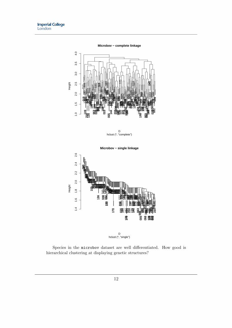
We will try to describe the genetic variability in the cat colonies of Nancyusing clustering methods. First, we need to compute a distance matrix. Re-place missing data in nancycats using na.replace, and then compute theEuclidean distances between individuals using dist on the table of relativeallele frequencies ($tab of the object in which NAs have been replaced). Usehclust to compute a clustering with complete linkage, and one with singlelinkage. How do they compare? How would you interprete these graphs?Can you assess the number of actual genetic clusters in these data?
As a comparison, repeat these analyses with the dataset microbov, whichcontains genotypes of various cattle breeds in France and Africa.
11
017
018
019
191
180
125
119
123
035
061
205
218
220
048
143
223
137
118
121
186
193
188
156
235
207
208 13
213
916
210
919
5 067 21
005
307
006
311
300
600
811
520
918
502
202
5 012
028
026
032
068
141
072
145
003
093
127
203
204
126
198
200
124
177
183
165
158
190
014
016 01
101
302
308
308
614
805
405
516
106
522
421
121
521
708
900
700
509
102
001
503
010
119
214
214
404
214
615
919
404
903
303
4 029 13
303
110
8 027
232
233 1
99 236
128
225
120
122
187
074
140
189
136
147
004
229
230
171
078
079
076
085
009
155
231
237
087
116
212
213
216
206
043
075
099
100
094
098
105
160
164
066
051
069
057
221
222
024
021
226 11
414
916
604
613
809
509
611
215
204
410
711
009
713
413
503
703
8 179
181 084
154
157
058
104
153
150
151
060
178
172
175
173
167
169
176
050
117
010
202
196
197 12
913
013
103
604
1 228
234
102
219
001
002
047
040
056
062
081
184
227
064
201
059
092
045
090
174
071
080
103
111
052
088
082
039
073
168
170
214
077
182
106
163
1.0
1.5
2.0
2.5
3.0
3.5
4.0
Microbov − complete linkage
hclust (*, "complete")D
Hei
ght
093
090
191
112
110
171
148
067
185
168
057
017
011
003
161
024
180
127
183
224
223
215
209
194
181
179
159
103
111
086
070
192
037
038
035
031
018
054
055 2
0210
117
421
421
020
619
518
616
613
613
413
512
410
809
709
609
508
908
408
306
005
305
004
904
804
504
613
803
402
901
901
011
414
9 033
152
154
153
150
151
066
109
027
193
081
042
146 17
722
110
215
712
621
721
120
820
019
818
818
717
217
514
713
313
208
711
611
506
109
207
108
007
907
605
104
404
303
604
101
503
001
603
201
202
802
602
202
502
122
601
416
016
410
420
515
616
313
916
2 235
085
170
167
173
169
176
013
023
107
069
222
212
207
213
216
204
203
196
197
165
129
128
125
119
123
088
075
142
144
068
141
072
145
074
065
059
058
052
047
008
117
006
063
113
094
106
099
100
098
105
007
005
091
143
020
232
233
236
199
064
201
228
078
077
182 0
4005
606
214
018
9 082
039
073
155
004
158
137
190
122
120
118
121
009
178
229
230
219
225
220
218
001
002
184
227 2
34 131
130
231
2371.4
1.6
1.8
2.0
2.2
2.4
2.6
Microbov − single linkage
hclust (*, "single")D
Hei
ght
Species in the microbov dataset are well differentiated. How good ishierarchical clustering at displaying genetic structures?
12
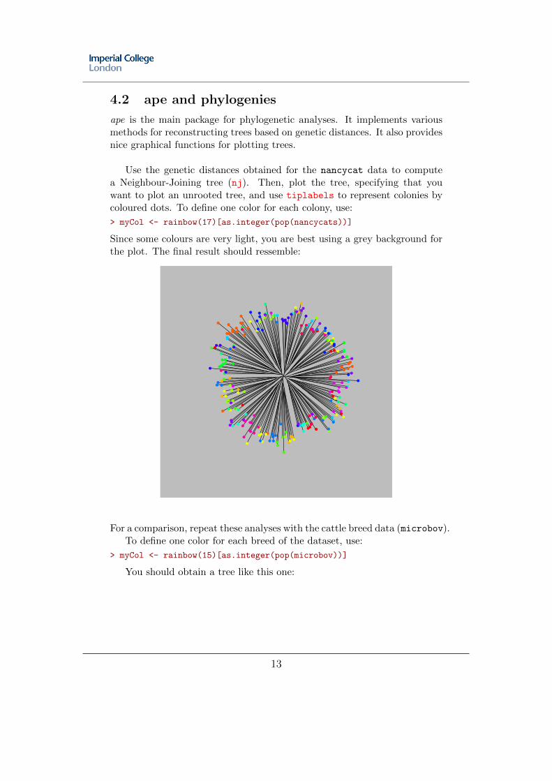
4.2 ape and phylogenies
ape is the main package for phylogenetic analyses. It implements variousmethods for reconstructing trees based on genetic distances. It also providesnice graphical functions for plotting trees.
Use the genetic distances obtained for the nancycat data to computea Neighbour-Joining tree (nj). Then, plot the tree, specifying that youwant to plot an unrooted tree, and use tiplabels to represent colonies bycoloured dots. To define one color for each colony, use:
> myCol <- rainbow(17)[as.integer(pop(nancycats))]
Since some colours are very light, you are best using a grey background forthe plot. The final result should ressemble:
●●
●
●●
●
●
●
●
●
●
●
●
●
●
●●
●●
●
●
●
●
●●
●
●
●
●
●
●
●
●●
●
●
●
●
●
●
●
●●
●
●
●
●
●
●
●
●
●
●
●●
●
●
●●
●
●
●●
●●
●
●
●
●
● ●
●
●
●
●
●
●●●
● ●
●
●
●
●
●
●
●
●
●
●
●
●
●●●
●
●
● ●
●
●
●
●
●
●
●
●
●
●
●
●
●
●
●
●
●
●
●●
●●
●
●
●
●
●
●
●
●●
●
●
●●
●
●
●
●
●●
●
●
●
●
●
●
●
●
●
●
●
● ●
●
●
●●
●
●
●
●
●
●
●●
●
●
●
●
●
●●
●●
●
●
●
●
●
●
●
●
●
●
●●
●
●
●●
●
●
●
●
●●
●
●
●
● ●
● ●
●
●
●
●
●
●●
●
●
●
●
●
●
●
●●
●
●
●
●
●
● ●
●
●●
●
●●
●●
●
●
For a comparison, repeat these analyses with the cattle breed data (microbov).To define one color for each breed of the dataset, use:
> myCol <- rainbow(15)[as.integer(pop(microbov))]
You should obtain a tree like this one:
13

●
●
●●
●
●
●
●●
●
●
●●
●
●
●●
●
●
●●
●●
●● ●
●
●
●●
●
●
●
●
●●
●
●
●●
●● ●●
●
●
●
●
●●
●●●
●
●
●●
●
●
●
●
● ●
●
●
●
●
● ●
●
●
●
●●●
●●
● ●
●
●
● ●
●
●
●
●
●
●
●
●
●
●
●
●
●●
●
●
●
●
●
●
●
●●●
●
●
●●
●
●● ●●●●
●
●
●
●
●
●●●●
●● ●
●
●●●●●
●
●
●●
●
●
●
●
●
●
●●
●●
●
●●
●
●
●
●
●
●
●●
●●
●●●
●
●
●
●
●
●●●
●●
●●● ●
●●
●●
●
●
●●
●
●
●
●
●
●
● ●
●
●
●
●
●
● ●●
●
●
●
●●
●
●
●
●
●
●
●
●
●●
●
●
●
●
●
●
●
●
●
●
●
●
● ●
●
●
●
●
●
●
●
●
●
●
●
●●
●
●
●
●
● ●
●
●●
●
●
●
●
●
●
●
●
●
●
●
●
●
●
●
●
●
●
●
●
●
●
●
●
●●
●
●●●
● ●
●
●
●
●●
●●●
●
●●●●●
●
●
●
●
●
●
●●●
●●
●●
● ●
●●
●●
●
●
●
●
●●●
●
●●
●
●
●
●
●●
●
●
●
●
●
● ●
●
●
●
●
●
●
●
●
●
●
●
●●
●
●
●
●
●
●
●
●
●
●
●
●
●●
●
●
●
●
●
●
●
●
●
●
●
●
●
●
●
●
●
●
●
●
●
● ●
●●
●
●
●
●
●
●●
●
●
●
●
●
●
●●
●
●●
●
●
●
●
● ●●
●
●
●
●●
●
●
●●
●●
●
●●● ●●
●
●
●
●●● ●
●● ●
●
●
●
●
●
●
●
●●
●
●
●●
●
●●
●
●
●
●
●●
●
●●
●
●
●
● ●
●
●
●●
●
●
●
●● ●
●
●●
●
●
●
●
●
●
●
●
●
●
●
●
●
●
●
●
●
●
●
●
● ●
●
●
●
●
●
●
●
●
●
●
●
●
●●
●
●
●
●
●
●
●
●
●
●
●●
●
●
●
●●
●
●
●●
●
●
●●
●
●
●
●
●
●
●
●
●
●
●
●
●
●●
●●
●●
●
●
●
●
● ●●●
●
●
●
●
●
●
●
●
●
●
● ●●●
●●
●
●●
●
●● ●
●
●
●
●
●
●
●●
●●
●
●
●●
●●●
●●
●●●
●
●
●
●
●●
●
●●●
●●
●
● ●
●
●●
●
●
●
●●
●
●
●
●●
●
●
●
●
●●
●
●
● ●
●●●
●
●
●
●
●
●
●
●
●
●
●
●
●●
●
●
●
●
●
●
●
●
●
●
●
●
●
●●
●●
●
●
●
● ●
●
●●
●
There are two species, Bos taurus and Bos indicus, in these cattle breeds;the species information is stored in microbov$other$spe. Use the same ap-proach to represent the species information on the tips of the tree. Is thisclassification reflected by a clear-cut structure on the tree?
The quality of a tree is unfortunately rarely questioned in terms of howwell the real distances are represented by the tree. The literature is evenfull of examples of analyses based on distances computed from trees, whilethe original distances that had generated the tree could have been used. Asimple way of assessing how good a tree is at representing a set of distancesis simply comparing the original distances to the reconstructed distances(sum of branch lengths between tips). The latter can be computed usingcophenetic. Use this function to plot both distances (microbov data), afterconverting the distances into vectors using as.vector; you should obtainthe following figure:
14
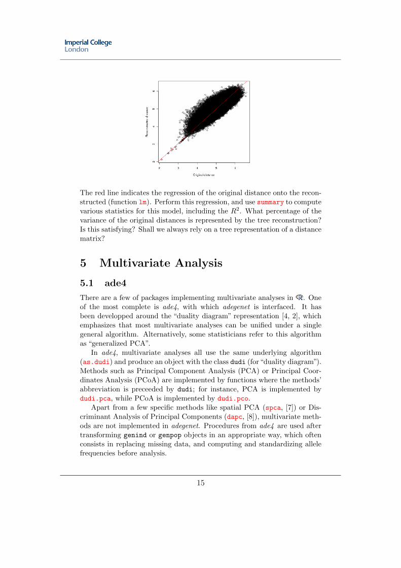
The red line indicates the regression of the original distance onto the recon-structed (function lm). Perform this regression, and use summary to computevarious statistics for this model, including the R2. What percentage of thevariance of the original distances is represented by the tree reconstruction?Is this satisfying? Shall we always rely on a tree representation of a distancematrix?
5 Multivariate Analysis
5.1 ade4
There are a few of packages implementing multivariate analyses in . Oneof the most complete is ade4, with which adegenet is interfaced. It hasbeen developped around the “duality diagram” representation [4, 2], whichemphasizes that most multivariate analyses can be unified under a singlegeneral algorithm. Alternatively, some statisticians refer to this algorithmas “generalized PCA”.
In ade4, multivariate analyses all use the same underlying algorithm(as.dudi) and produce an object with the class dudi (for“duality diagram”).Methods such as Principal Component Analysis (PCA) or Principal Coor-dinates Analysis (PCoA) are implemented by functions where the methods’abbreviation is preceeded by dudi; for instance, PCA is implemented bydudi.pca, while PCoA is implemented by dudi.pco.
Apart from a few specific methods like spatial PCA (spca, [7]) or Dis-criminant Analysis of Principal Components (dapc, [8]), multivariate meth-ods are not implemented in adegenet. Procedures from ade4 are used aftertransforming genind or genpop objects in an appropriate way, which oftenconsists in replacing missing data, and computing and standardizing allelefrequencies before analysis.
15
5.2 Principal Component Analysis (PCA)
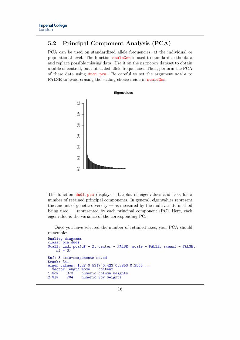
PCA can be used on standardized allele frequencies, at the individual orpopulational level. The function scaleGen is used to standardize the dataand replace possible missing data. Use it on the microbov dataset to obtaina table of centred, but not scaled allele frequencies. Then, perform the PCAof these data using dudi.pca. Be careful to set the argument scale toFALSE to avoid erasing the scaling choice made in scaleGen.
Eigenvalues
0.0
0.2
0.4
0.6
0.8
1.0
1.2
The function dudi.pca displays a barplot of eigenvalues and asks for anumber of retained principal components. In general, eigenvalues representthe amount of genetic diversity — as measured by the multivariate methodbeing used — represented by each principal component (PC). Here, eacheigenvalue is the variance of the corresponding PC.
Once you have selected the number of retained axes, your PCA shouldressemble:
Duality diagrammclass: pca dudi$call: dudi.pca(df = X, center = FALSE, scale = FALSE, scannf = FALSE,
nf = 3)
$nf: 3 axis-components saved$rank: 341eigen values: 1.27 0.5317 0.423 0.2853 0.2565 ...vector length mode content
1 $cw 373 numeric column weights2 $lw 704 numeric row weights
16
3 $eig 341 numeric eigen values
data.frame nrow ncol content1 $tab 704 373 modified array2 $li 704 3 row coordinates3 $l1 704 3 row normed scores4 $co 373 3 column coordinates5 $c1 373 3 column normed scoresother elements: cent norm
The printing of dudi object is not always explicit. The essential itemsfor the analyses we will use are:
? $eig: eigenvalues of the analysis
? $c1: principal axes, containing the loadings of the variables (alleles)
? $li: principal components, containing the scores of the individuals
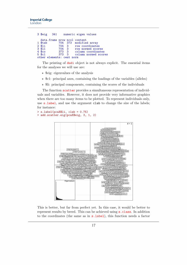
The function scatter provides a simultaneous representation of individ-uals and variables. However, it does not provide very informative graphicswhen there are too many items to be plotted. To represent individuals only,use s.label, and use the argument clab to change the size of the labels;for instance:
> s.label(pcaX$li, clab = 0.75)> add.scatter.eig(pcaX$eig, 3, 1, 2)
d = 1
AFBIBOR9503
AFBIBOR9504
AFBIBOR9505
AFBIBOR9506
AFBIBOR9507
AFBIBOR9508
AFBIBOR9509
AFBIBOR9510 AFBIBOR9511
AFBIBOR9512
AFBIBOR9513 AFBIBOR9514 AFBIBOR9515
AFBIBOR9516 AFBIBOR9517
AFBIBOR9518
AFBIBOR9519
AFBIBOR9520
AFBIBOR9521
AFBIBOR9522
AFBIBOR9523
AFBIBOR9524 AFBIBOR9525 AFBIBOR9526
AFBIBOR9527 AFBIBOR9528
AFBIBOR9529 AFBIBOR9530 AFBIBOR9531 AFBIBOR9532
AFBIBOR9533
AFBIBOR9534
AFBIBOR9535 AFBIBOR9536
AFBIBOR9537
AFBIBOR9538 AFBIBOR9539 AFBIBOR9540
AFBIBOR9541
AFBIBOR9542 AFBIBOR9543
AFBIBOR9544
AFBIBOR9545
AFBIBOR9546
AFBIBOR9547
AFBIBOR9548
AFBIBOR9549
AFBIBOR9550
AFBIBOR9551 AFBIBOR9552
AFBIZEB9453 AFBIZEB9454
AFBIZEB9455 AFBIZEB9456
AFBIZEB9457
AFBIZEB9458
AFBIZEB9459
AFBIZEB9460
AFBIZEB9461
AFBIZEB9462
AFBIZEB9463
AFBIZEB9464
AFBIZEB9465
AFBIZEB9466 AFBIZEB9467 AFBIZEB9468
AFBIZEB9469
AFBIZEB9470
AFBIZEB9471 AFBIZEB9472
AFBIZEB9473
AFBIZEB9474
AFBIZEB9475
AFBIZEB9476
AFBIZEB9477
AFBIZEB9478
AFBIZEB9479
AFBIZEB9480
AFBIZEB9481 AFBIZEB9482 AFBIZEB9483
AFBIZEB9484
AFBIZEB9485
AFBIZEB9486 AFBIZEB9487
AFBIZEB9488
AFBIZEB9489
AFBIZEB9490
AFBIZEB9491
AFBIZEB9492
AFBIZEB9493 AFBIZEB9494
AFBIZEB9495
AFBIZEB9496
AFBIZEB9497
AFBIZEB9498
AFBIZEB9499
AFBIZEB9500
AFBIZEB9501 AFBIZEB9502
AFBTLAG9402
AFBTLAG9403 AFBTLAG9404
AFBTLAG9405
AFBTLAG9406
AFBTLAG9407 AFBTLAG9408
AFBTLAG9409
AFBTLAG9410
AFBTLAG9411
AFBTLAG9412
AFBTLAG9413 AFBTLAG9414
AFBTLAG9415
AFBTLAG9416
AFBTLAG9417
AFBTLAG9418 AFBTLAG9419 AFBTLAG9420
AFBTLAG9421
AFBTLAG9422
AFBTLAG9423 AFBTLAG9424
AFBTLAG9425
AFBTLAG9426 AFBTLAG9427 AFBTLAG9428 AFBTLAG9429
AFBTLAG9430 AFBTLAG9431
AFBTLAG9432 AFBTLAG9433 AFBTLAG9434
AFBTLAG9435
AFBTLAG9436 AFBTLAG9437
AFBTLAG9438
AFBTLAG9439
AFBTLAG9440
AFBTLAG9441
AFBTLAG9442
AFBTLAG9443
AFBTLAG9444
AFBTLAG9445
AFBTLAG9446
AFBTLAG9447
AFBTLAG9448
AFBTLAG9449
AFBTLAG9450
AFBTLAG9451
AFBTLAG9452
AFBTND202 AFBTND205
AFBTND206 AFBTND207
AFBTND208
AFBTND209
AFBTND211
AFBTND212
AFBTND213 AFBTND214
AFBTND215
AFBTND216
AFBTND217
AFBTND221 AFBTND222
AFBTND223
AFBTND233
AFBTND241
AFBTND242
AFBTND244 AFBTND248 AFBTND253
AFBTND254
AFBTND255 AFBTND257
AFBTND258
AFBTND259 AFBTND284
AFBTND285
AFBTND292
AFBTSOM9352 AFBTSOM9353
AFBTSOM9354
AFBTSOM9355 AFBTSOM9356
AFBTSOM9357
AFBTSOM9358
AFBTSOM9359
AFBTSOM9360
AFBTSOM9361 AFBTSOM9362
AFBTSOM9363 AFBTSOM9364 AFBTSOM9365
AFBTSOM9366
AFBTSOM9367
AFBTSOM9368 AFBTSOM9369
AFBTSOM9370
AFBTSOM9371
AFBTSOM9372
AFBTSOM9373
AFBTSOM9374
AFBTSOM9375
AFBTSOM9376 AFBTSOM9377
AFBTSOM9378
AFBTSOM9379
AFBTSOM9380 AFBTSOM9381
AFBTSOM9382
AFBTSOM9383
AFBTSOM9384
AFBTSOM9385
AFBTSOM9386
AFBTSOM9387
AFBTSOM9388 AFBTSOM9389
AFBTSOM9390 AFBTSOM9391
AFBTSOM9392
AFBTSOM9393
AFBTSOM9394
AFBTSOM9395
AFBTSOM9396
AFBTSOM9397 AFBTSOM9398
AFBTSOM9399 AFBTSOM9400
AFBTSOM9401
FRBTAUB9061 FRBTAUB9062 FRBTAUB9063
FRBTAUB9064
FRBTAUB9065
FRBTAUB9066
FRBTAUB9067 FRBTAUB9068
FRBTAUB9069 FRBTAUB9070
FRBTAUB9071
FRBTAUB9072
FRBTAUB9073 FRBTAUB9074 FRBTAUB9075
FRBTAUB9076
FRBTAUB9077
FRBTAUB9078 FRBTAUB9079
FRBTAUB9081
FRBTAUB9208
FRBTAUB9210
FRBTAUB9211 FRBTAUB9212
FRBTAUB9213
FRBTAUB9216
FRBTAUB9218
FRBTAUB9219 FRBTAUB9220
FRBTAUB9221
FRBTAUB9222
FRBTAUB9223 FRBTAUB9224 FRBTAUB9225
FRBTAUB9226 FRBTAUB9227 FRBTAUB9228
FRBTAUB9229 FRBTAUB9230 FRBTAUB9231 FRBTAUB9232
FRBTAUB9234
FRBTAUB9235
FRBTAUB9237 FRBTAUB9238
FRBTAUB9286
FRBTAUB9287 FRBTAUB9288
FRBTAUB9289
FRBTAUB9290
FRBTBAZ15654
FRBTBAZ15655
FRBTBAZ25576
FRBTBAZ25578 FRBTBAZ25950 FRBTBAZ25954
FRBTBAZ25956
FRBTBAZ25957 FRBTBAZ26078 FRBTBAZ26092
FRBTBAZ26097 FRBTBAZ26110 FRBTBAZ26112
FRBTBAZ26352 FRBTBAZ26354
FRBTBAZ26375 FRBTBAZ26386
FRBTBAZ26388
FRBTBAZ26396
FRBTBAZ26400
FRBTBAZ26401
FRBTBAZ26403
FRBTBAZ26439
FRBTBAZ26457 FRBTBAZ26463
FRBTBAZ26469
FRBTBAZ29244
FRBTBAZ29246
FRBTBAZ29247
FRBTBAZ29253
FRBTBAZ29254
FRBTBAZ29259
FRBTBAZ29261
FRBTBAZ29262 FRBTBAZ29272
FRBTBAZ29281 FRBTBAZ29598
FRBTBAZ30418 FRBTBAZ30420
FRBTBAZ30421
FRBTBAZ30429
FRBTBAZ30436
FRBTBAZ30440
FRBTBAZ30531 FRBTBAZ30533
FRBTBAZ30539
FRBTBAZ30540
FRBTBDA29851
FRBTBDA29852
FRBTBDA29853 FRBTBDA29854 FRBTBDA29855
FRBTBDA29856 FRBTBDA29857
FRBTBDA29858 FRBTBDA29859
FRBTBDA29860
FRBTBDA29861
FRBTBDA29862 FRBTBDA29863
FRBTBDA29864 FRBTBDA29865
FRBTBDA29866
FRBTBDA29868 FRBTBDA29869
FRBTBDA29870
FRBTBDA29872
FRBTBDA29873
FRBTBDA29874 FRBTBDA29875
FRBTBDA29877
FRBTBDA29878
FRBTBDA29879 FRBTBDA29880
FRBTBDA29881 FRBTBDA29882 FRBTBDA35243
FRBTBDA35244
FRBTBDA35245
FRBTBDA35248 FRBTBDA35255
FRBTBDA35256
FRBTBDA35258
FRBTBDA35259
FRBTBDA35260
FRBTBDA35262
FRBTBDA35267 FRBTBDA35268 FRBTBDA35269
FRBTBDA35274
FRBTBDA35278
FRBTBDA35280
FRBTBDA35281
FRBTBDA35283
FRBTBDA35284 FRBTBDA35286 FRBTBDA35379 FRBTBDA35446
FRBTBDA35485 FRBTBDA35864
FRBTBDA35877
FRBTBDA35899
FRBTBDA35916
FRBTBDA35931
FRBTBDA35941 FRBTBDA35955
FRBTBDA36120
FRBTBDA36124
FRBTBPN1870
FRBTBPN1872 FRBTBPN1873
FRBTBPN1875
FRBTBPN1876
FRBTBPN1877
FRBTBPN1894
FRBTBPN1895 FRBTBPN1896
FRBTBPN1897
FRBTBPN1898
FRBTBPN1899
FRBTBPN1901 FRBTBPN1902
FRBTBPN1904
FRBTBPN1906
FRBTBPN1907
FRBTBPN1910 FRBTBPN1911
FRBTBPN1913 FRBTBPN1914 FRBTBPN1915
FRBTBPN1927
FRBTBPN1928
FRBTBPN1930
FRBTBPN1932
FRBTBPN1934
FRBTBPN1935
FRBTBPN1937 FRBTBPN25810
FRBTBPN25811
FRBTCHA15946
FRBTCHA15957 FRBTCHA15985
FRBTCHA15994
FRBTCHA25009
FRBTCHA25015
FRBTCHA25018 FRBTCHA25024
FRBTCHA25069
FRBTCHA25295
FRBTCHA25322 FRBTCHA25326
FRBTCHA25390 FRBTCHA25513
FRBTCHA25543 FRBTCHA25654 FRBTCHA25995 FRBTCHA26011
FRBTCHA26014 FRBTCHA26040
FRBTCHA26054
FRBTCHA26074
FRBTCHA26193 FRBTCHA26196
FRBTCHA26199
FRBTCHA26202
FRBTCHA26205
FRBTCHA26246
FRBTCHA26274
FRBTCHA26285
FRBTCHA26783
FRBTCHA26784
FRBTCHA26785 FRBTCHA26786 FRBTCHA26789 FRBTCHA26790 FRBTCHA26792 FRBTCHA26793
FRBTCHA26797
FRBTCHA26798
FRBTCHA26800
FRBTCHA30335
FRBTCHA30341
FRBTCHA30344 FRBTCHA30353 FRBTCHA30356
FRBTCHA30373
FRBTCHA30382 FRBTCHA30391
FRBTCHA30878
FRBTCHA30879
FRBTCHA30884 FRBTCHA30886
FRBTCHA30893
FRBTCHA30896 FRBTGAS14180
FRBTGAS14183
FRBTGAS14184
FRBTGAS14185
FRBTGAS14186
FRBTGAS14187
FRBTGAS14188 FRBTGAS9049
FRBTGAS9050 FRBTGAS9051
FRBTGAS9052 FRBTGAS9053
FRBTGAS9054
FRBTGAS9055 FRBTGAS9056
FRBTGAS9057
FRBTGAS9058
FRBTGAS9059
FRBTGAS9060
FRBTGAS9170
FRBTGAS9171
FRBTGAS9172
FRBTGAS9173
FRBTGAS9174
FRBTGAS9175
FRBTGAS9176
FRBTGAS9177
FRBTGAS9178
FRBTGAS9179 FRBTGAS9180
FRBTGAS9181 FRBTGAS9182
FRBTGAS9183
FRBTGAS9184
FRBTGAS9185 FRBTGAS9186
FRBTGAS9188
FRBTGAS9189
FRBTGAS9190
FRBTGAS9193
FRBTGAS9195
FRBTGAS9197
FRBTGAS9198
FRBTGAS9199 FRBTGAS9200 FRBTGAS9201 FRBTGAS9202 FRBTGAS9203
FRBTGAS9204
FRBTGAS9205 FRBTLIM3001
FRBTLIM30816 FRBTLIM30817
FRBTLIM30818
FRBTLIM30819 FRBTLIM30820
FRBTLIM30821
FRBTLIM30822
FRBTLIM30823
FRBTLIM30824 FRBTLIM30825
FRBTLIM30826 FRBTLIM30827 FRBTLIM30828 FRBTLIM30829 FRBTLIM30830
FRBTLIM30831
FRBTLIM30832 FRBTLIM30833
FRBTLIM30834
FRBTLIM30835
FRBTLIM30836
FRBTLIM30837 FRBTLIM30838 FRBTLIM30839
FRBTLIM30840
FRBTLIM30841 FRBTLIM30842
FRBTLIM30843 FRBTLIM30844 FRBTLIM30845
FRBTLIM30846
FRBTLIM30847
FRBTLIM30848 FRBTLIM30849
FRBTLIM30850
FRBTLIM30851
FRBTLIM30852
FRBTLIM30853
FRBTLIM30854
FRBTLIM30855
FRBTLIM30856
FRBTLIM30857
FRBTLIM30858 FRBTLIM30859 FRBTLIM30860
FRBTLIM5133
FRBTLIM5135
FRBTLIM5136
FRBTLIM5137
FRBTMA25273 FRBTMA25278
FRBTMA25282
FRBTMA25298
FRBTMA25382
FRBTMA25387
FRBTMA25409
FRBTMA25412
FRBTMA25418
FRBTMA25423
FRBTMA25428
FRBTMA25433
FRBTMA25436 FRBTMA25439 FRBTMA25488
FRBTMA25522 FRBTMA25530
FRBTMA25588
FRBTMA25594 FRBTMA25612
FRBTMA25614 FRBTMA25684
FRBTMA25820
FRBTMA25896
FRBTMA25902
FRBTMA25917 FRBTMA25922 FRBTMA25978 FRBTMA25982
FRBTMA26019 FRBTMA26022 FRBTMA26035
FRBTMA26168
FRBTMA26232
FRBTMA26280
FRBTMA26321 FRBTMA26491 FRBTMA29561
FRBTMA29571
FRBTMA29572 FRBTMA29806
FRBTMA29809
FRBTMA29812 FRBTMA29819 FRBTMA29943
FRBTMA29945
FRBTMA29948
FRBTMA29950 FRBTMA29952
FRBTMBE1496 FRBTMBE1497 FRBTMBE1502
FRBTMBE1503
FRBTMBE1505 FRBTMBE1506
FRBTMBE1507
FRBTMBE1508 FRBTMBE1510
FRBTMBE1511 FRBTMBE1513
FRBTMBE1514
FRBTMBE1516
FRBTMBE1517 FRBTMBE1519
FRBTMBE1520
FRBTMBE1523
FRBTMBE1529 FRBTMBE1531
FRBTMBE1532
FRBTMBE1534
FRBTMBE1535
FRBTMBE1536
FRBTMBE1538
FRBTMBE1540 FRBTMBE1541
FRBTMBE1544
FRBTMBE1547 FRBTMBE1548
FRBTMBE1549
FRBTSAL9087 FRBTSAL9088
FRBTSAL9089
FRBTSAL9090
FRBTSAL9091
FRBTSAL9093 FRBTSAL9094 FRBTSAL9095
FRBTSAL9096
FRBTSAL9097 FRBTSAL9099
FRBTSAL9100
FRBTSAL9101
FRBTSAL9102
FRBTSAL9103
FRBTSAL9241
FRBTSAL9242
FRBTSAL9243
FRBTSAL9245
FRBTSAL9246 FRBTSAL9247
FRBTSAL9248 FRBTSAL9249
FRBTSAL9250
FRBTSAL9251
FRBTSAL9252
FRBTSAL9253
FRBTSAL9255
FRBTSAL9256
FRBTSAL9257
FRBTSAL9258
FRBTSAL9259
FRBTSAL9260 FRBTSAL9261
FRBTSAL9262
FRBTSAL9265
FRBTSAL9266
FRBTSAL9267
FRBTSAL9268
FRBTSAL9270 FRBTSAL9271
FRBTSAL9272 FRBTSAL9273
FRBTSAL9275 FRBTSAL9276 FRBTSAL9277
FRBTSAL9280
FRBTSAL9283
FRBTSAL9284 FRBTSAL9285
Eigenvalues
This is better, but far from perfect yet. In this case, it would be better torepresent results by breed. This can be achieved using s.class. In additionto the coordinates (the same as in s.label), this function needs a factor
17
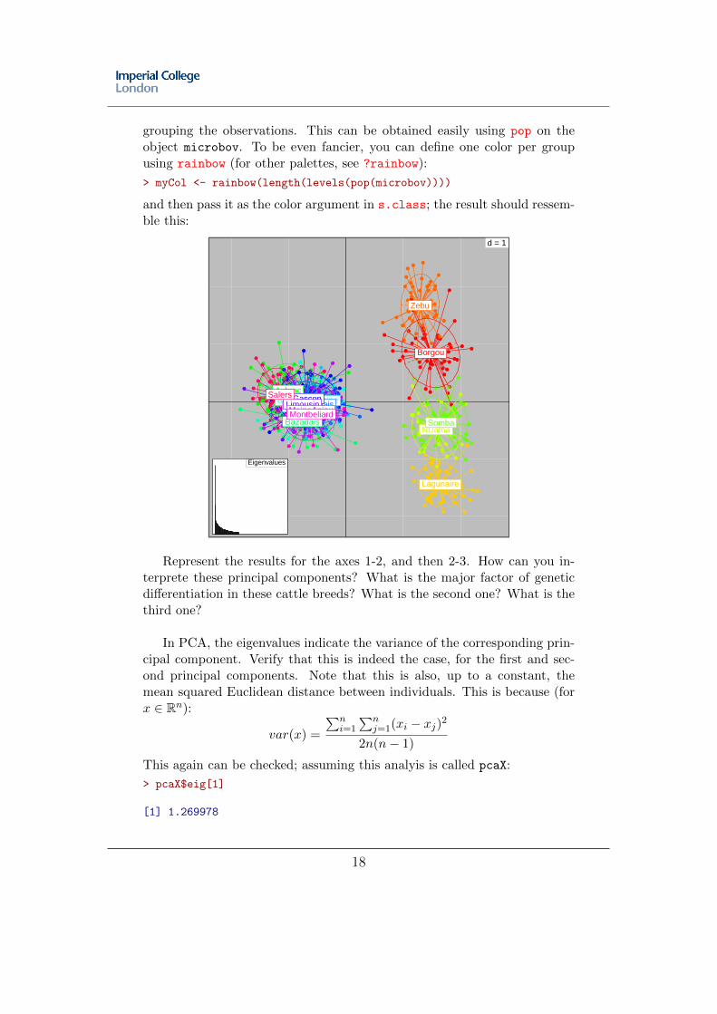
grouping the observations. This can be obtained easily using pop on theobject microbov. To be even fancier, you can define one color per groupusing rainbow (for other palettes, see ?rainbow):
> myCol <- rainbow(length(levels(pop(microbov))))
and then pass it as the color argument in s.class; the result should ressem-ble this:
d = 1
●
●
●
●
●
●
●
●
●
●
●● ●
●
●
●
●
●
●
●
●
●● ●
●
●
●●●
●
●
●
●●
●
●
●
●
●
●
●
●
●
●
●
●
●
●
●
●
●
●
●
●
●
●
●
●
●
●
●
●
●
●
●●
●
●
●
●
●
●
●
●
●
●
●
●
●
● ●
●
●
●
●
●
●
●
●
●
●
●
●
●
●
●
●
●
●
●
●
●
●
●
●
●
●
●
●
●
●
●●
●
●
●
●
●●
●
●
●
●
●
●●
●●
●●
● ●●
●
●●
●
●
●
●
●
●
●
●
●
●
●
●
●
●
●
●
●
●
●
●
●
●
●
●
●
●
●
●
●
●
●
●
●
●
●
● ●
●
●
●
●
●●
●
●
●
●
●
●
●
●
●
●
●
●
●
● ●●
●
●
●●
●
●
●
●
●
●
● ●
●
●
●
●
●
●
●
●
●
●
●
●
●
●
●
●
●
●
●
●
●
●●
●
●
●●
●
●
●
●
●
●
●
●
●
●
●●
●
●
●
●
●
●
●
●
●
●
●
●
●
●
●
●
●●
●
●
●●
●
● ●●
●
●
●●
●
●●
●
●
●
●
●
●●
●
●
●
●●
●
●●
●●
●●
●
●
●
●
●
●
●
●
●
●
●
●
●
●
●
●
●
●
●●
●●
●
●
●
●
●
●
●
●
●
●
●●
●
●
●
● ●
●
●
●
●
●
●
●
●●
●
●
●
●
●
●
●
●
●
●
●●
●
●
● ●
●
●
●
●
●
●
●●
●
●
●
●
●
●●
●●
●
●●
●
●
●
●
●
●
●
●
●●
●
●
●
●
● ●
●
●
●
●
●
●
●
●
●
●
●●●
●
●
●
●
●
●
●
●
●
●
●
●
●
●
●
● ●
●
●
●
●
●
●
●●
●
●
●
●
●
●
●●
●
●
●
●
●
●
●
●
●
●●●●●
●
●
●
●
●
●●
●
●
●
●
●
●
●
●
●
●
●
●
●
●
●
●
●●
●
●
●
●
●
●
●
●
●
●
●
●
●
●
●
●
●
●
●
●
●
●
● ●
●
●
●
●
●
●
●
●
●
●
●
●●● ●
●
●
●
●
●
●
●
● ●
●
●
●
●●
●●
●
● ●
●
●●
●
●
●
●
●●
●
●
●
●
●●
●
●
●●
●
●
●
●
●
●
●
●
● ●
●
●
●
●
●
●
●
●
●
●
●
●
●
●
●
●
●
●
●●
●
●
●
●
●
●
●
●
●
●
●●
●
●
● ●
●
●
●
●
●●
●
●
●●
●
●●
●
●
●
●
●
●
●●
●
●
●
●
●●
●
●
●
●
●
●
●
●
●●
●
●
●
●
●
●
●
●
●●
●
●●
●
●
●
●●
●
●
●●
●
●
●
●
●
●
●
●
●
●
●
●
●
●
●
●
●
●
●
●
●
●●
●
●
●
●
●
●
●
●
●
●●
●
●
●
●
●
Borgou
Zebu
Lagunaire
NDama Somba
Aubrac
Bazadais
BlondeAquitaine BretPieNoire Charolais
Gascon Limousin MaineAnjou Montbeliard
Salers
Eigenvalues
Represent the results for the axes 1-2, and then 2-3. How can you in-terprete these principal components? What is the major factor of geneticdifferentiation in these cattle breeds? What is the second one? What is thethird one?
In PCA, the eigenvalues indicate the variance of the corresponding prin-cipal component. Verify that this is indeed the case, for the first and sec-ond principal components. Note that this is also, up to a constant, themean squared Euclidean distance between individuals. This is because (forx ∈ Rn):
var(x) =
∑ni=1
∑nj=1(xi − xj)
2
2n(n− 1)
This again can be checked; assuming this analyis is called pcaX:
> pcaX$eig[1]
[1] 1.269978
18
> pc1 <- pcaX$li[, 1]> n <- length(pc1)> 0.5 * mean(dist(pc1)^2) * ((n - 1)/n)
[1] 1.269978
We sometimes want to express eigenvalues as a percentage of the totalvariation in the data. What is the percentage of variance explained by thefirst three eigenvalues?
Allele contributions can sometimes be informative. The basic graphicsfor representing allele loadings is s.arrow. Use it to represent the resultsof the PCA; is this informative? An alternative is offered by loadingplot,which represents one axis at a time. Use it to represent the squared loadingsof the analysis; how does it compare to previous representation? The func-tion returns invisibly some information; adapting the arguments and savingthe returned value, identify the 2% alleles contributing most to showing thediversity within African breeds. You should find:
[1] "ETH152.197" "INRA32.178" "HEL13.182" "MM12.119" "CSRM60.093"[6] "TGLA227.079" "TGLA126.119" "TGLA122.150"
5.3 Principal Coordinates Analysis (PCoA)
We have just seen that the variance is, up to a constant, equal to the meansquared distance between all pairs of observations. Therefore, maximizingthe variance along an axis should be exactly the same as maximizing thesum of all squared Euclidean distances. This latter maximization is theobjective of Principal Coordinates Analysis (PCoA), also known as Met-ric Multidimensional Scaling (MDS). This method is implemented in ade4by dudi.pco. After scaling the relative allele frequencies of the microbov
dataset, perform this analysis.Represent the principal components ($li) of this analysis and compare
them to the PCs of the previous PCA. What is the correlation betweenthem? Compare the scatter plots of both analyses; are there any differ-ences? In practice, in which cases should we prefer PCA over PCoA, or thecontrary?
As an exercise, compute genetic similarities based on the proportion ofshared alleles (propShared) on the microbov data. Transform the similar-ities into a distance (no dedicated function for this), and perform a PCoAof the resulting distance. Is this distance Euclidean? If not, it needs tobe. Transform it into an Euclidean distance (using cailliez) and redo thePCoA. How do the results compare to the previous analyses?
19
References
[1] D. Chessel, A-B. Dufour, and J. Thioulouse. The ade4 package-I- one-table methods. R News, 4:5–10, 2004.
[2] S. Dray and A.-B. Dufour. The ade4 package: implementing the dualitydiagram for ecologists. Journal of Statistical Software, 22(4):1–20, 2007.
[3] S. Dray, A.-B. Dufour, and D. Chessel. The ade4 package - II: Two-table and K-table methods. R News, 7:47–54, 2007.
[4] Y. Escoufier. The duality diagramm : a means of better practicalapplications. In P. Legendre and L. Legendre, editors, Development innumerical ecology, pages 139–156. NATO advanced Institute , Serie G.Springer Verlag, Berlin, 1987.
[5] J. Goudet. HIERFSTAT, a package for R to compute and test hierar-chical F-statistics. Molecular Ecology Notes, 5:184–186, 2005.
[6] T. Jombart. adegenet: a R package for the multivariate analysis ofgenetic markers. Bioinformatics, 24:1403–1405, 2008.
[7] T. Jombart, S. Devillard, A.-B. Dufour, and D. Pontier. Revealingcryptic spatial patterns in genetic variability by a new multivariatemethod. Heredity, 101:92–103, 2008.
[8] Thibaut Jombart, Sebastien Devillard, and Francois Balloux. Discrim-inant analysis of principal components: a new method for the analysisof genetically structured populations. BMC Genetics, 11(1):94, 2010.
[9] E. Paradis, J. Claude, and K. Strimmer. APE: analyses of phylogeneticsand evolution in R language. Bioinformatics, 20:289–290, 2004.
[10] R Development Core Team. R: A Language and Environment for Sta-tistical Computing. R Foundation for Statistical Computing, Vienna,Austria, 2009. ISBN 3-900051-07-0.
[11] G. R. Warnes. The genetics package. R News, 3(1):9–13, 2003.
20
Recommended