1
INTRODUCTION TO CLINICAL RESEARCH
Introduction to Linear Regression
Gayane Yenokyan, MD, MPH, PhD
Associate Director, Biostatistics Center
Department of Biostatistics, JHSPH
1
Outline
1. Studying association between (health) outcomes and (health) determinants
2. Correlation
3. Goals of Linear regression: – Estimation: Characterizing relationships
– Prediction: Predicting average Y from X(s)
4. Future topics: multiple linear regression, assumptions, complex relationships
2
Introduction
• A statistical method for describing a “response”or “outcome” variable (usually denoted by Y) as a simple function of “explanatory” or “predictor”variables (X)
• Continuously measured outcomes (“linear”)
– No gaps
– Total lung capacity (l) and height (m)
– Birthweight (g) and gestational age (mos)
– Systolic BP (mm Hg) and salt intake (g)
– Systolic BP (mm Hg) and drug (trt, placebo)
33
2
Introduction
• The term “regression” was first used by Francis Galton in 19th
century
• Described biological phenomenon that heights of descendants of tall parents tend to be lower on average or to regress towards the mean
• In this case, interest is to predict son’s height based on father’s height
44
Heights of Fathers and Sons I
5
Heights of Fathers and Sons II
6
3
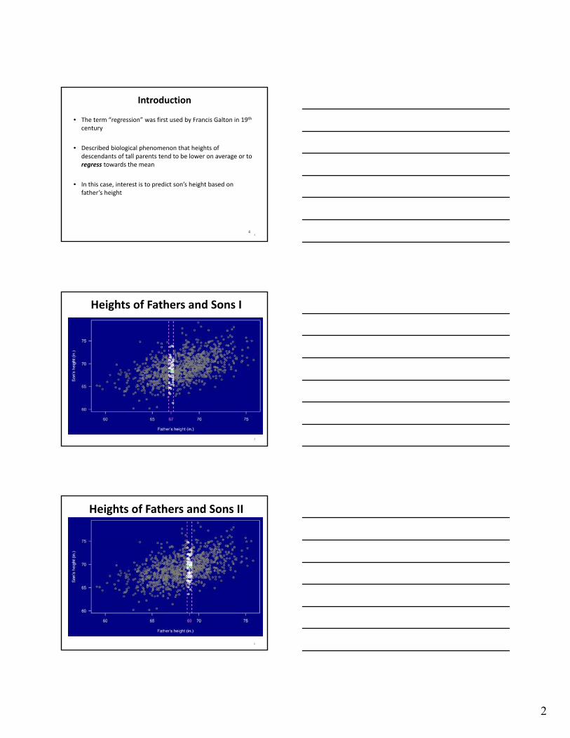
Heights of Fathers and Sons III
7
Heights of Sons vs. Fathers: Regression Line I
8
Heights of Fathers vs. Sons: Regression Line II
9

4
Concept of Regression
• Regression concerns predicting Y from X.
• There are two regression lines.
• The regression effect: – Tall fathers, on average, have sons who are not so tall.
– Short fathers, on average, have sons who are not so short.
• The regression fallacy: assigning some deeper (causal) meaning to the regression effect.
10
Example: Association of total lung capacity with height
Study: 32 heart lung transplant recipients aged 11‐59 years
. list tlc height age in 1/10 +---------------------+ | tlc height age | |---------------------| 1. | 3.41 138 11 | 2. | 3.4 149 35 | 3. | 8.05 162 20 | 4. | 5.73 160 23 | 5. | 4.1 157 16 | |---------------------| 6. | 5.44 166 40 | 7. | 7.2 177 39 | 8. | 6 173 29 | 9. | 4.55 152 16 | 10. | 4.83 177 35 | +---------------------+
11
Correlation vs. Regression
• Two analyses to study association of continuously measured health outcomes and health determinants
– Correlation analysis: Concerned with measuring the strength and direction of the association betweenvariables. The correlation of X and Y (Y and X).
– Linear regression: Concerned with predicting the value of one variable based on (given) the value of the othervariable. The regression of Y on X.
1212
5
13
Some specific names for “correlation” in one’s data:
• r
• Sample correlation coefficient
• Pearson correlation coefficient
• Product moment correlation coefficient
Correlation Coefficient
13
14
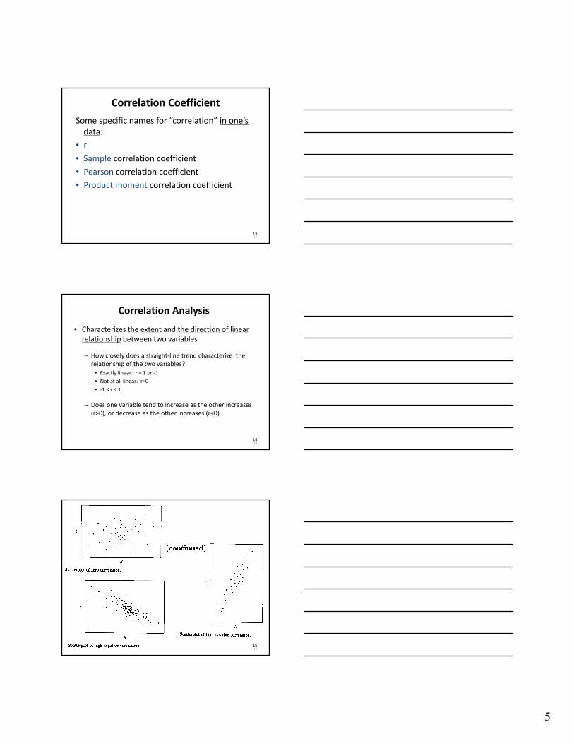
Correlation Analysis
• Characterizes the extent and the direction of linear relationship between two variables
– How closely does a straight‐line trend characterize the relationship of the two variables?
• Exactly linear: r = 1 or ‐1
• Not at all linear: r=0
• ‐1 ≤ r ≤ 1
– Does one variable tend to increase as the other increases (r>0), or decrease as the other increases (r<0)
14
1515
6
16
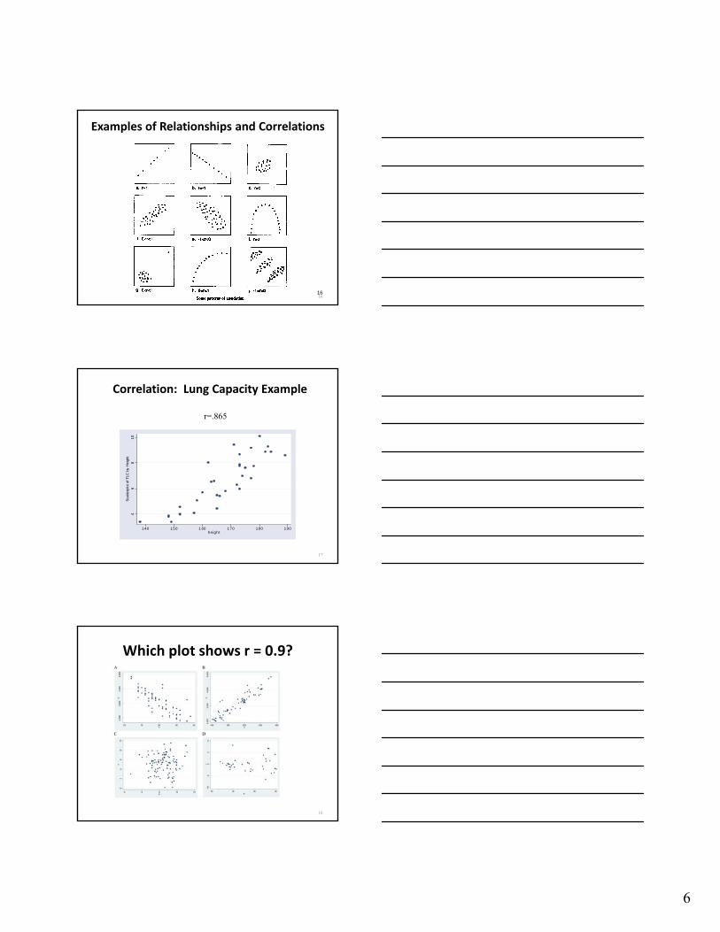
Examples of Relationships and Correlations
16
46
810
Sca
tterp
lot o
f TLC
by
Hei
ght
140 150 1 60 170 180 190height
Correlation: Lung Capacity Example
r=.865
17
Which plot shows r = 0.9?
18
7
19
FYI: Sample Correlation Formula
Heuristic: If I draw a straight line through the vertical middle of scatter of points created by plotting y versus x, r divides the SD of the heights of points on the line by the SD of the heights of the original points
19
20
Correlation – Closing Remarks
• The value of r is independent of the units used to measure the variables
• The value of r can be substantially influenced bya small fraction of outliers
• The value of r considered “large” varies over science disciplines– Physics : r=0.9
– Biology : r=0.5
– Sociology : r=0.2
• r is a “guess” at a population analog
20
21
What Is Regression Analysis?
A statistical method for describing a “response” or “outcome” variable (usually denoted by Y) as a simple function of “explanatory” or “predictor” variables (X)
Goals of regression analysis:
1. Prediction: predict average response (Y) for a given X (or Xs)Example research question: How precisely can we predict a given person’s Y
with his/her X
2. Estimation: describe the relationship between average Y and X. Parameters: slope and interceptExample research question: What is the relationship between average Y and
X?
• We care about “slope”—size, direction
• Slope=0 corresponds to “no association”
8
22
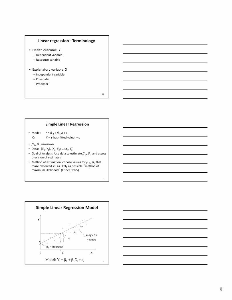
Linear regression –Terminology
• Health outcome, Y
– Dependent variable
– Response variable
• Explanatory variable, X
– Independent variable
– Covariate
– Predictor
22
23
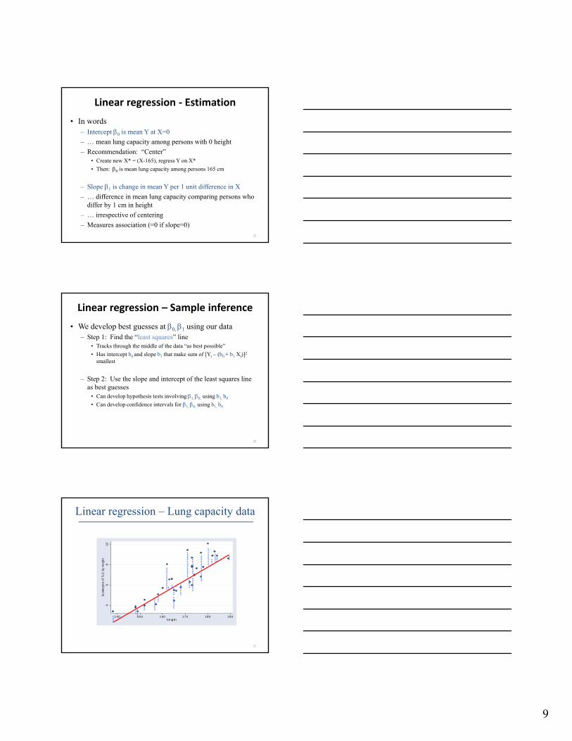
Simple Linear Regression
• Model: Y = 0 + 1 X + Or Y = Y‐hat (fitted value) +
• 0, 1 unknown
• Data: (X1, Y1), (X2, Y2) … (Xn, Yn)
• Goal of Analysis: Use data to estimate 0, 1 and assess precision of estimates
• Method of estimation: choose values for 0 , 1 that make observed Ys as likely as possible “method of maximum likelihood” (Fisher, 1925)
y
xi
yi
i
0 = Intercept
1 = y / x
= slope
X
Y
x
0
Simple Linear Regression Model
Model: Yi = 0 + 1Xi + i 24
9
Linear regression ‐ Estimation
• In words – Intercept 0 is mean Y at X=0
– … mean lung capacity among persons with 0 height
– Recommendation: “Center”• Create new X* = (X-165), regress Y on X*
• Then: 0 is mean lung capacity among persons 165 cm
– Slope 1 is change in mean Y per 1 unit difference in X
– … difference in mean lung capacity comparing persons who differ by 1 cm in height
– … irrespective of centering
– Measures association (=0 if slope=0)
25
Linear regression – Sample inference
• We develop best guesses at 0, 1 using our data – Step 1: Find the “least squares” line
• Tracks through the middle of the data “as best possible”
• Has intercept b0 and slope b1 that make sum of [Yi – (b0 + b1 Xi)]2
smallest
– Step 2: Use the slope and intercept of the least squares line as best guesses
• Can develop hypothesis tests involving 1, 0, using b1, b0
• Can develop confidence intervals for 1, 0, using b1, b0
26
46
81
0S
catte
rplo
t o
f T
LC
by
He
igh
t
140 150 1 60 170 180 190he ight
Linear regression – Lung capacity data
27
10
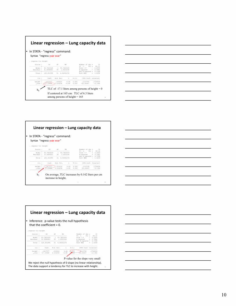
Linear regression – Lung capacity data
• In STATA ‐ “regress” command:
Syntax “regress yvar xvar”
. regress tlc height Source | SS df MS Number of obs = 32 -------------+------------------------------ F( 1, 30) = 89.12 Model | 93.7825029 1 93.7825029 Prob > F = 0.0000 Residual | 31.5694921 30 1.0523164 R-squared = 0.7482 -------------+------------------------------ Adj R-squared = 0.7398 Total | 125.351995 31 4.04361274 Root MSE = 1.0258 ------------------------------------------------------------------------------ tlc | Coef. Std. Err. t P>|t| [95% Conf. Interval] -------------+---------------------------------------------------------------- height | .1417377 .015014 9.44 0.000 .1110749 .1724004 _cons | -17.10484 2.516234 -6.80 0.000 -22.24367 -11.966 ------------------------------------------------------------------------------
TLC of -17.1 liters among persons of height = 0
If centered at 165 cm: TLC of 6.3 liters among persons of height = 165
b0
28
Linear regression – Lung capacity data
• In STATA ‐ “regress” command:
Syntax “regress yvar xvar”
. regress tlc height Source | SS df MS Number of obs = 32 -------------+------------------------------ F( 1, 30) = 89.12 Model | 93.7825029 1 93.7825029 Prob > F = 0.0000 Residual | 31.5694921 30 1.0523164 R-squared = 0.7482 -------------+------------------------------ Adj R-squared = 0.7398 Total | 125.351995 31 4.04361274 Root MSE = 1.0258 ------------------------------------------------------------------------------ tlc | Coef. Std. Err. t P>|t| [95% Conf. Interval] -------------+---------------------------------------------------------------- height | .1417377 .015014 9.44 0.000 .1110749 .1724004 _cons | -17.10484 2.516234 -6.80 0.000 -22.24367 -11.966 ------------------------------------------------------------------------------
On average, TLC increases by 0.142 liters per cm increase in height, or equivalently, by 1.42 liters per 10 cm increase in height.
b1
29
Linear regression – Lung capacity data
• Inference: p‐value tests the null hypothesis that the coefficient = 0.
. regress tlc height Source | SS df MS Number of obs = 32 -------------+------------------------------ F( 1, 30) = 89.12 Model | 93.7825029 1 93.7825029 Prob > F = 0.0000 Residual | 31.5694921 30 1.0523164 R-squared = 0.7482 -------------+------------------------------ Adj R-squared = 0.7398 Total | 125.351995 31 4.04361274 Root MSE = 1.0258 ------------------------------------------------------------------------------ tlc | Coef. Std. Err. t P>|t| [95% Conf. Interval] -------------+---------------------------------------------------------------- height | .1417377 .015014 9.44 0.000 .1110749 .1724004 _cons | -17.10484 2.516234 -6.80 0.000 -22.24367 -11.966 ------------------------------------------------------------------------------
We reject the null hypothesis of 0 slope (no linear relationship). The data support a tendency for TLC to increase with height.
P-value for the slope very small
30
11
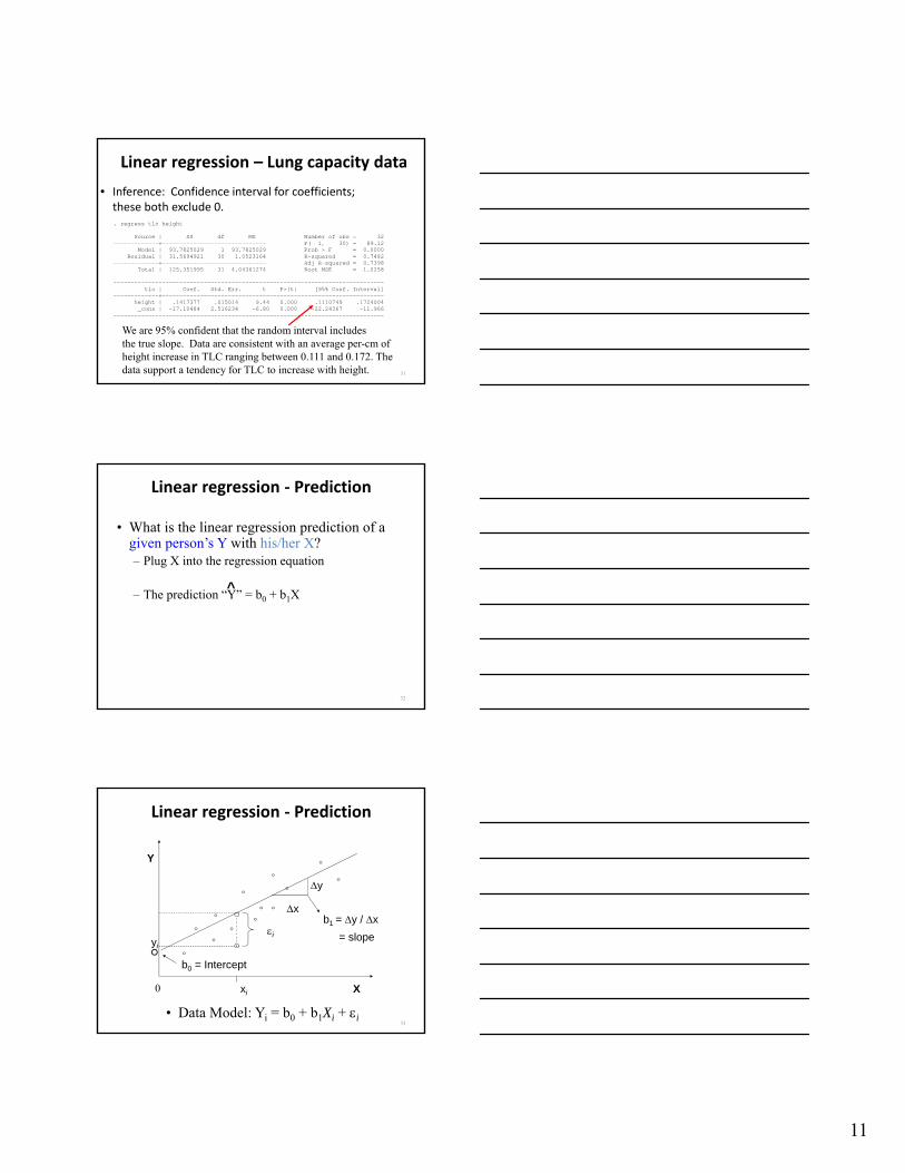
Linear regression – Lung capacity data
• Inference: Confidence interval for coefficients; these both exclude 0.. regress tlc height Source | SS df MS Number of obs = 32 -------------+------------------------------ F( 1, 30) = 89.12 Model | 93.7825029 1 93.7825029 Prob > F = 0.0000 Residual | 31.5694921 30 1.0523164 R-squared = 0.7482 -------------+------------------------------ Adj R-squared = 0.7398 Total | 125.351995 31 4.04361274 Root MSE = 1.0258 ------------------------------------------------------------------------------ tlc | Coef. Std. Err. t P>|t| [95% Conf. Interval] -------------+---------------------------------------------------------------- height | .1417377 .015014 9.44 0.000 .1110749 .1724004 _cons | -17.10484 2.516234 -6.80 0.000 -22.24367 -11.966 ------------------------------------------------------------------------------
We are 95% confident that the random interval includes the true slope. Data are consistent with an average per-cm of height increase in TLC ranging between 0.111 and 0.172. The data support a tendency for TLC to increase with height. 31
Linear regression ‐ Prediction
• What is the linear regression prediction of a given person’s Y with his/her X?– Plug X into the regression equation
– The prediction “Y” = b0 + b1X^
32
y
xi
yi
i
b0 = Intercept
b1 = y / x
= slope
X
Y
x
0
Linear regression ‐ Prediction
• Data Model: Yi = b0 + b1Xi + i33
12
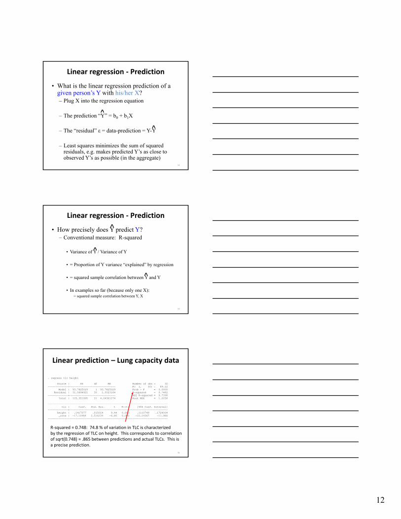
Linear regression ‐ Prediction
• What is the linear regression prediction of a given person’s Y with his/her X?– Plug X into the regression equation
– The prediction “Y” = b0 + b1X
– The “residual” ε = data-prediction = Y-Y
– Least squares minimizes the sum of squared residuals, e.g. makes predicted Y’s as close to observed Y’s as possible (in the aggregate)
^
^
34
Linear regression ‐ Prediction
• How precisely does Y predict Y?– Conventional measure: R-squared
• Variance of Y / Variance of Y
• = Proportion of Y variance “explained” by regression
• = squared sample correlation between Y and Y
• In examples so far (because only one X): = squared sample correlation between Y, X
^
^
^
35
Linear prediction – Lung capacity data
. regress tlc height Source | SS df MS Number of obs = 32 -------------+------------------------------ F( 1, 30) = 89.12 Model | 93.7825029 1 93.7825029 Prob > F = 0.0000 Residual | 31.5694921 30 1.0523164 R-squared = 0.7482 -------------+------------------------------ Adj R-squared = 0.7398 Total | 125.351995 31 4.04361274 Root MSE = 1.0258 ------------------------------------------------------------------------------ tlc | Coef. Std. Err. t P>|t| [95% Conf. Interval] -------------+---------------------------------------------------------------- height | .1417377 .015014 9.44 0.000 .1110749 .1724004 _cons | -17.10484 2.516234 -6.80 0.000 -22.24367 -11.966 ------------------------------------------------------------------------------
R‐squared = 0.748: 74.8 % of variation in TLC is characterized by the regression of TLC on height. This corresponds to correlationof sqrt(0.748) = .865 between predictions and actual TLCs. This isa precise prediction.
36
13
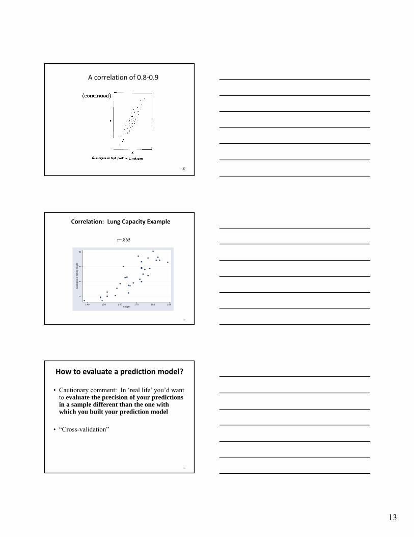
37
A correlation of 0.8‐0.9
37
46
810
Sca
tterp
lot o
f TLC
by
Hei
ght
140 150 1 60 170 180 190he ight
Correlation: Lung Capacity Example
r=.865
38
How to evaluate a prediction model?
• Cautionary comment: In ‘real life’ you’d want to evaluate the precision of your predictions in a sample different than the one with which you built your prediction model
• “Cross-validation”
39
14
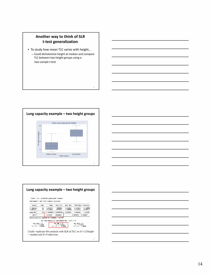
• To study how mean TLC varies with height…
– Could dichotomize height at median and compare TLC between two height groups using a
two‐sample t‐test
Another way to think of SLRt‐test generalization
40
46
810
TLC
(To
tal L
ung
Cap
acity
)
Median or Below Above MedianHeight Category
Total Lung Capacity By Height
Lung capacity example – two height groups
41
Lung capacity example – two height groups
Could ~replicate this analysis with SLR of TLC on X=1 if height > median and X=0 otherwise
42

15
More advanced topicsRegression with more than one predictor
• “Multiple” linear regression– More than one X variable (ex.: height, age)
– With only 1 X we have “simple” linear regression
• Yi = 0 + 1Xi1 + 2Xi2 + … + pXip + i
• Intercept 0 is mean Y for persons with all Xs=0
• Slope k is change in mean Y per 1 unit difference in Xk among persons identical on all other Xs
43
More advanced topicsRegression with more than one predictor
• Slope k is change in mean Y per 1 unit difference in Xk among persons identical on all other Xs– i.e. holding all other Xs constant
– i.e. “controlling for” all other Xs
• Fitted slopes for a given predictor in a simple linear regression and a multiple linear regression controlling for other predictors do NOT have to be the same
– We’ll learn why in the lecture on confounding
44
Model Checking
• Most published regression analyses make statistical assumptions
• Why this matters: p‐values and confidence intervals may be wrong, and coefficient interpretation may be obscure, if assumptions aren’t approximately true
• Good research reports on analyses to check whether assumptions are met (“diagnostics”, “residual analysis”, “model checking/fit”, etc.)
45

16
Linear Regression Assumptions
• Units are sampled independently (no connections such as familial relationship, residential clustering, etc.)
• Posited model for average Y‐X relationship is correct
• Normally (Gaussian; bell‐shaped) distributed responses for each X
• Variability of responses (Ys) the same for all X46
Linear Regression Assumptions
02
04
06
08
01
00
20 30 40 50 60 70age
y Fitted values
-40
-20
02
04
0R
esid
ua
ls
20 30 40 50 60 70age
Assumptions well met:
47
Linear Regression Assumptions
Non‐normal responses per X
-10
010
20
30R
esid
ual
s
20 30 40 50 60 70age
204
060
80
100
20 30 40 50 60 70age
y2 Fitted values
48

17
Linear Regression Assumptions
Non‐constant variability of responses per X
20
40
608
01
001
20
20 30 40 50 60 70age
y3 Fitted values
-40
-20
02
04
06
0R
esid
ual
s
20 30 40 50 60 70age
49
Linear Regression Assumptions
50
Linear Regression Assumptions – Lung Capacity Example
-2-1
01
2R
esid
ual
s
140 150 160 170 180 190height
24
68
10
140 150 160 170 180 190height
tlc Fitted values
51

18
More advanced topicsTypes of relationships that can be studied
• ANOVA (multiple group differences)
• ANCOVA (different slopes per groups)– Effect modification: lecture to come
• Curves (polynomials, broken arrows, more)
• Etc.
52
What we talked about today
1. Studying association between (health) outcomes and (health) determinants
2. Correlation
3. Goals of Linear regression: – Estimation: Characterizing relationships
– Prediction: Predicting average Y from X
4. Future topics: multiple linear regression, assumptions, complex relationships
53
Acknowledgements
• Karen Bandeen‐Roche
• Marie Diener‐West
• Rick Thompson
• ICTR Leadership / Team
54
Recommended