Introduction to (Bayesian) Isotope Mixing Models
Eric Ward
Northwest Fisheries Science Center Seattle WA, USA
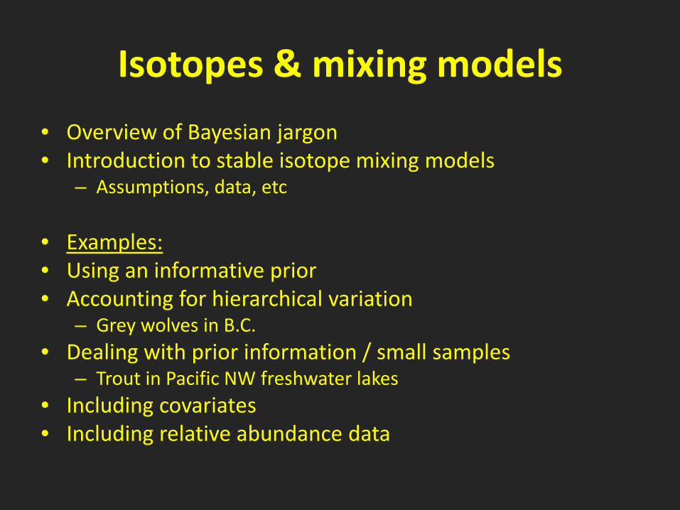
Isotopes & mixing models
• Overview of Bayesian jargon • Introduction to stable isotope mixing models
– Assumptions, data, etc
• Examples: • Using an informative prior • Accounting for hierarchical variation
– Grey wolves in B.C. • Dealing with prior information / small samples
– Trout in Pacific NW freshwater lakes • Including covariates • Including relative abundance data
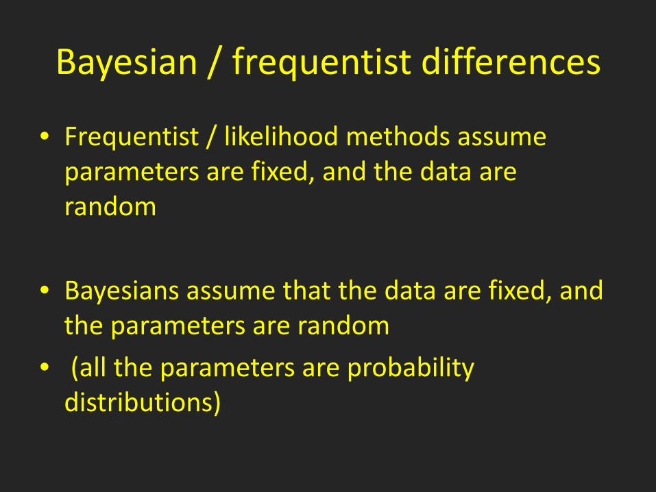
Bayesian / frequentist differences
• Frequentist / likelihood methods assume parameters are fixed, and the data are random
• Bayesians assume that the data are fixed, and the parameters are random
• (all the parameters are probability distributions)

Bayesian Jargon
• Prior: π(θ) – this is a probability distribution representing prior knowledge
• Likelihood: L(x|θ) – this is the likelihood of your data given the parameter
• Posterior = Pr(θ|x) ≈ π(θ)×L(x|θ)
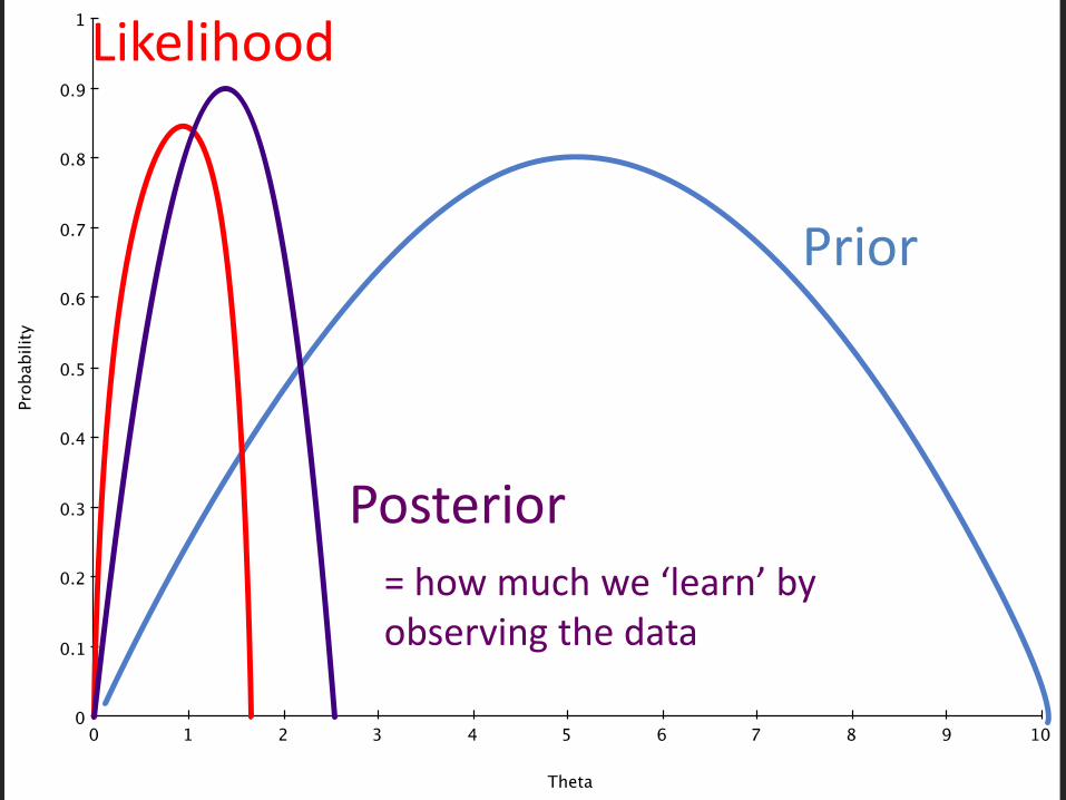
Prior
Posterior
Likelihood
= how much we ‘learn’ by observing the data
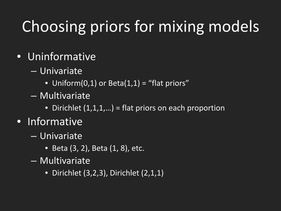
Choosing priors for mixing models
• Uninformative – Univariate
• Uniform(0,1) or Beta(1,1) = “flat priors”
– Multivariate • Dirichlet (1,1,1,…) = flat priors on each proportion
• Informative – Univariate
• Beta (3, 2), Beta (1, 8), etc.
– Multivariate • Dirichlet (3,2,3), Dirichlet (2,1,1)
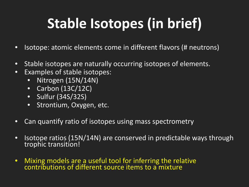
Stable Isotopes (in brief) • Isotope: atomic elements come in different flavors (# neutrons)
• Stable isotopes are naturally occurring isotopes of elements. • Examples of stable isotopes:
• Nitrogen (15N/14N) • Carbon (13C/12C) • Sulfur (34S/32S) • Strontium, Oxygen, etc.
• Can quantify ratio of isotopes using mass spectrometry
• Isotope ratios (15N/14N) are conserved in predictable ways through
trophic transition!
• Mixing models are a useful tool for inferring the relative contributions of different source items to a mixture
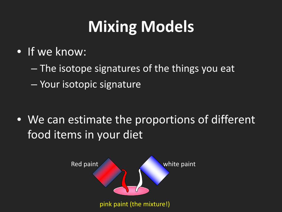
Mixing Models • If we know:
– The isotope signatures of the things you eat
– Your isotopic signature
• We can estimate the proportions of different food items in your diet
Red paint white paint
pink paint (the mixture!)
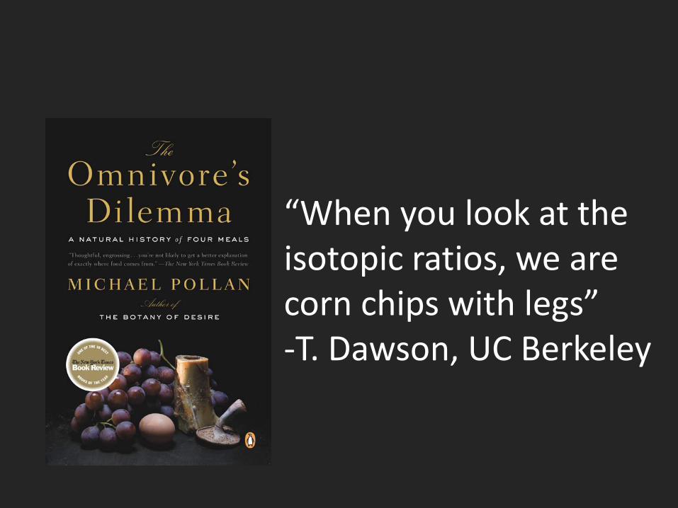
“When you look at the isotopic ratios, we are corn chips with legs” -T. Dawson, UC Berkeley
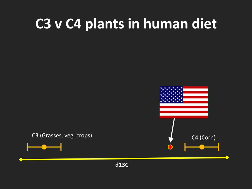
C3 v C4 plants in human diet
d13C
C4 (Corn) C3 (Grasses, veg. crops)
USA
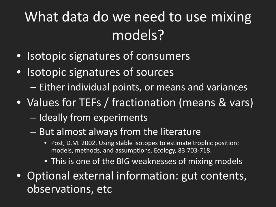
What data do we need to use mixing models?
• Isotopic signatures of consumers • Isotopic signatures of sources
– Either individual points, or means and variances
• Values for TEFs / fractionation (means & vars) – Ideally from experiments – But almost always from the literature
• Post, D.M. 2002. Using stable isotopes to estimate trophic position: models, methods, and assumptions. Ecology, 83:703-718.
• This is one of the BIG weaknesses of mixing models
• Optional external information: gut contents, observations, etc
C
Isot
ope
1 (e
.g. N
)
Isotope 2 (e.g. C)
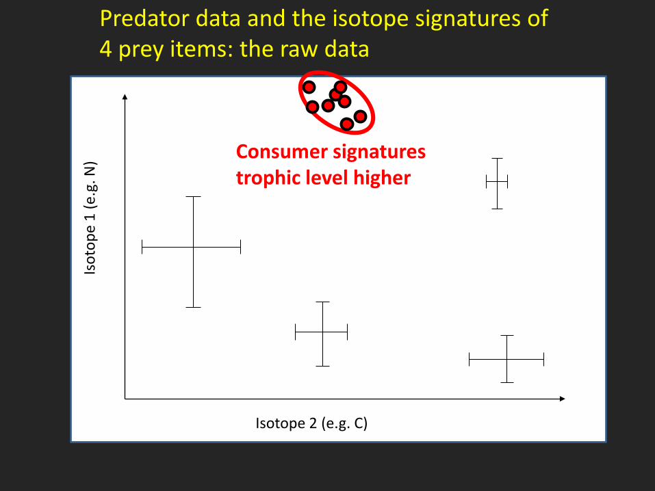
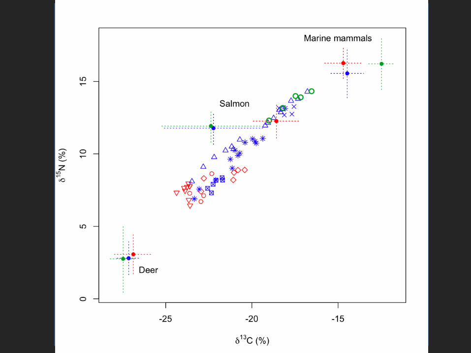
Predator data and the isotope signatures of 4 prey items: the raw data
Consumer signatures trophic level higher
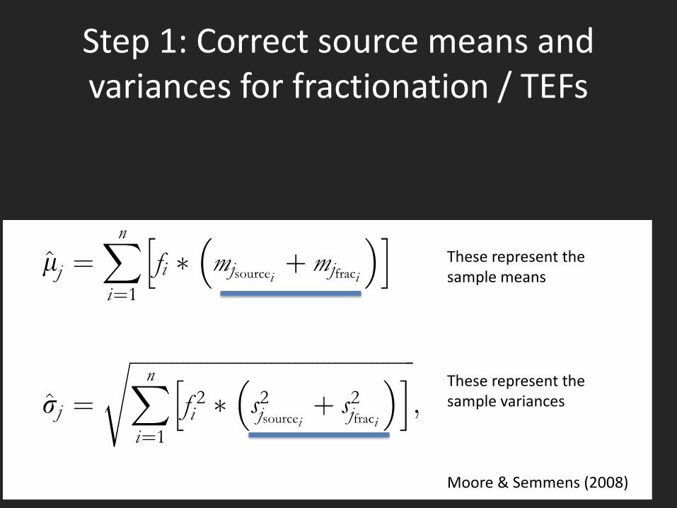
Step 1: Correct source means and variances for fractionation / TEFs
Moore & Semmens (2008)
These represent the sample variances
These represent the sample means
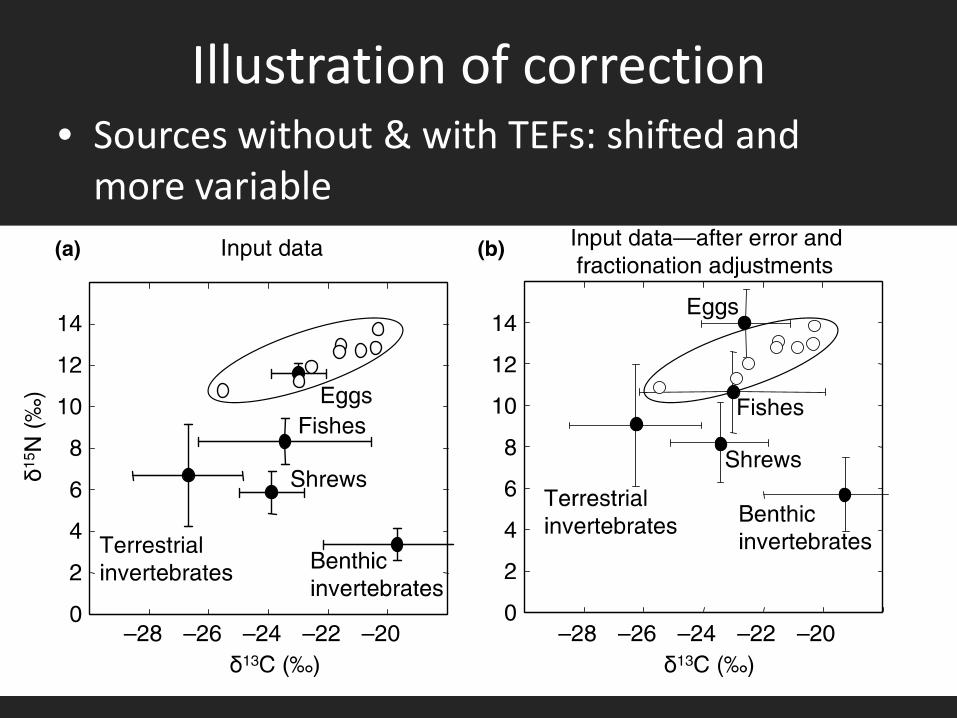
Illustration of correction • Sources without & with TEFs: shifted and
more variable
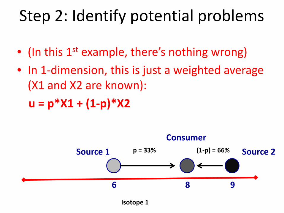
Step 2: Identify potential problems
Isotope 1
(1-p) = 66% p = 33%
• (In this 1st example, there’s nothing wrong)
• In 1-dimension, this is just a weighted average (X1 and X2 are known):
u = p*X1 + (1-p)*X2
Source 1 Source 2
Consumer
6 9 8
• Q: What is the value of mixing proportion p?
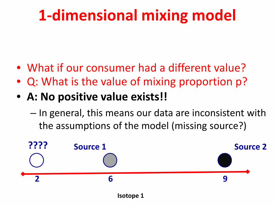
1-dimensional mixing model
• What if our consumer had a different value?
???? Source 2 Source 1
6 9 2
Isotope 1
• A: No positive value exists!! – In general, this means our data are inconsistent with
the assumptions of the model (missing source?)
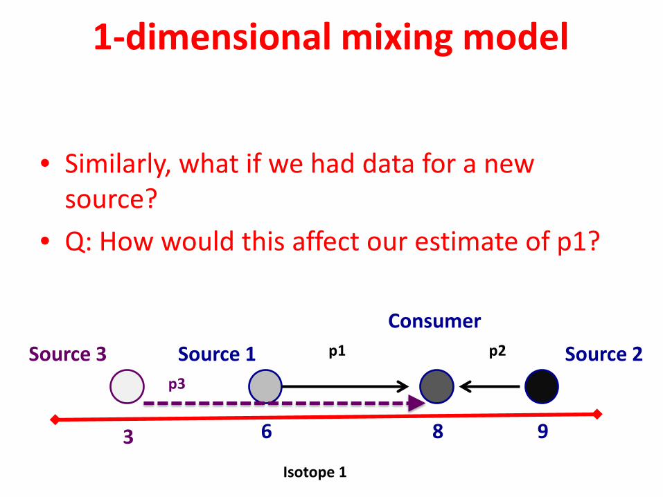
1-dimensional mixing model
Isotope 1
p2 p1
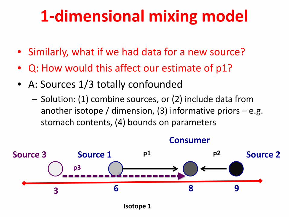
• Similarly, what if we had data for a new source?
• Q: How would this affect our estimate of p1?
Source 1 Source 2
Consumer
6 9 8
Source 3
3
p3
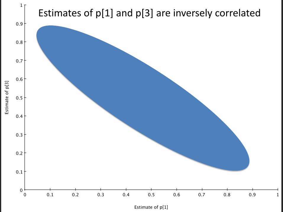
Estimates of p[1] and p[3] are inversely correlated
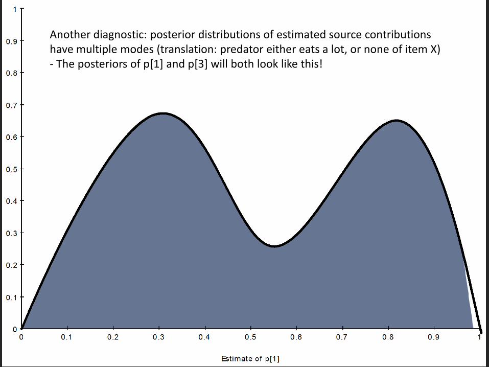
Another diagnostic: posterior distributions of estimated source contributions have multiple modes (translation: predator either eats a lot, or none of item X) - The posteriors of p[1] and p[3] will both look like this!
1-dimensional mixing model
Isotope 1
p2 p1
• Similarly, what if we had data for a new source?
• Q: How would this affect our estimate of p1?
• A: Sources 1/3 totally confounded – Solution: (1) combine sources, or (2) include data from
another isotope / dimension, (3) informative priors – e.g. stomach contents, (4) bounds on parameters
Source 1 Source 2
Consumer
6 9 8
Source 3
3
p3
Geometry in 2D can also be a problem
• Phillips and Gregg (2003)
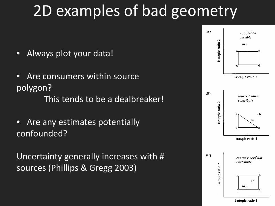
2D examples of bad geometry
• Always plot your data!
• Are consumers within source polygon? This tends to be a dealbreaker!
• Are any estimates potentially confounded? Uncertainty generally increases with # sources (Phillips & Gregg 2003)
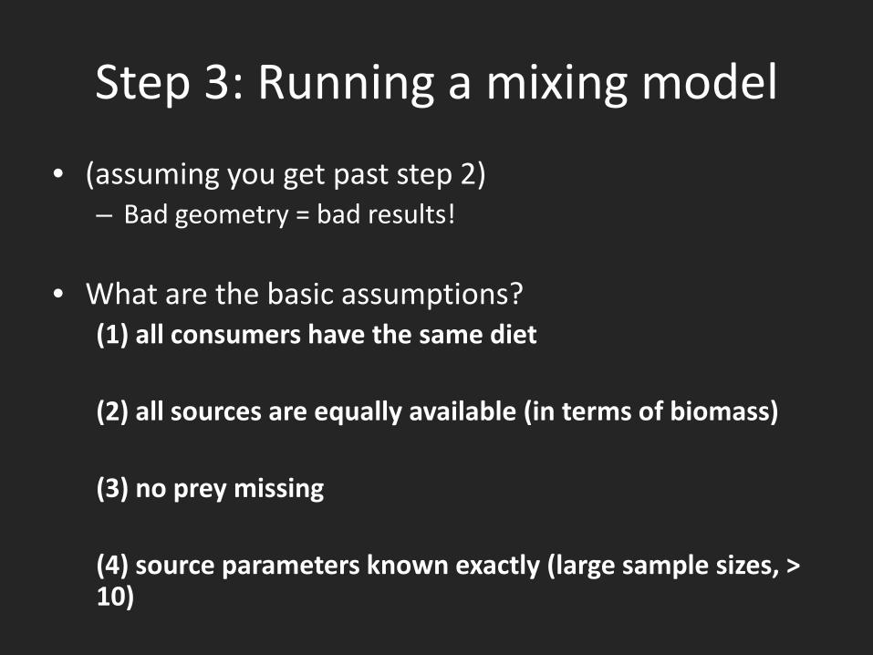
Step 3: Running a mixing model
• (assuming you get past step 2) – Bad geometry = bad results!
• What are the basic assumptions? (1) all consumers have the same diet (2) all sources are equally available (in terms of biomass) (3) no prey missing (4) source parameters known exactly (large sample sizes, > 10)
Isot
ope
1
Isotope 2
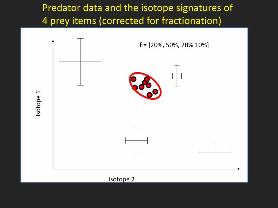
Predator data and the isotope signatures of 4 prey items (corrected for fractionation)
f = [20%, 50%, 20% 10%]
Isot
ope
1
Isotope 2
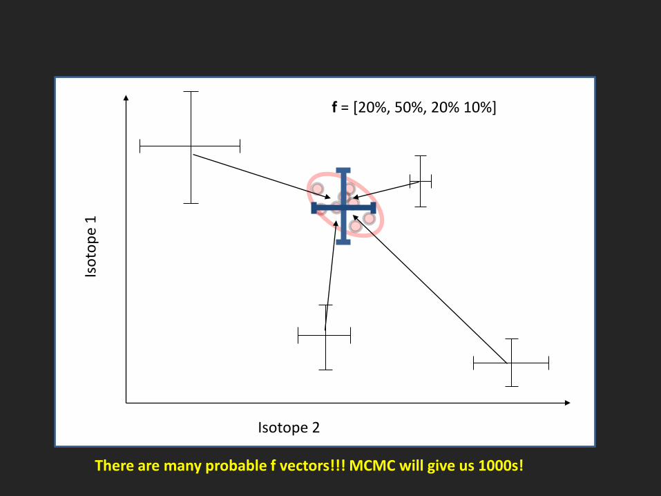
f = [20%, 50%, 20% 10%]
There are many probable f vectors!!! MCMC will give us 1000s!
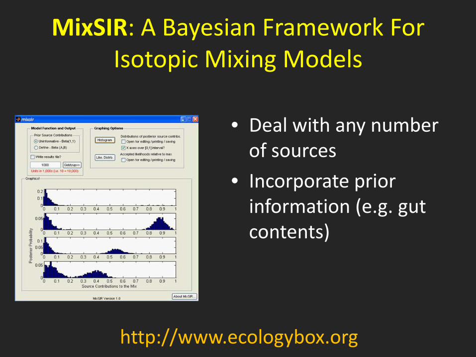
MixSIR: A Bayesian Framework For Isotopic Mixing Models
• Deal with any number of sources
• Incorporate prior information (e.g. gut contents)
http://www.ecologybox.org

Source: MixSIR manual, ecologybox.org

All the data together
What does MixSIR do?
• Implements the SIR algorithm – Sampling Importance Resampling
• Generates 1000s of independent samples from the posterior distribution of estimated source contributions (you specify # of samples)
• All vectors have to sum to 1!
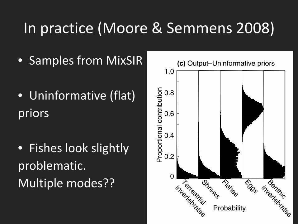
In practice (Moore & Semmens 2008)
• Samples from MixSIR
• Uninformative (flat) priors
• Fishes look slightly problematic. Multiple modes??
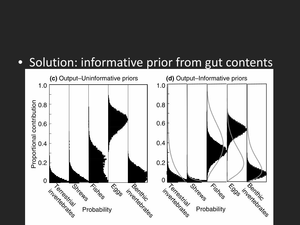
• Solution: informative prior from gut contents
Other examples
• Individual and group variation
• Uncertainty in sources
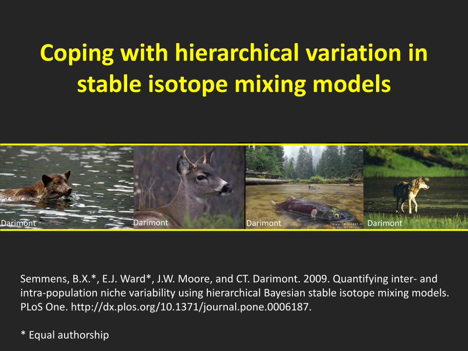
Coping with hierarchical variation in stable isotope mixing models
Semmens, B.X.*, E.J. Ward*, J.W. Moore, and CT. Darimont. 2009. Quantifying inter- and intra-population niche variability using hierarchical Bayesian stable isotope mixing models. PLoS One. http://dx.plos.org/10.1371/journal.pone.0006187. * Equal authorship
Darimont Darimont Darimont Darimont Darimont
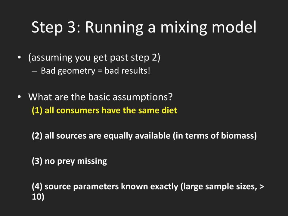
Step 3: Running a mixing model
• (assuming you get past step 2) – Bad geometry = bad results!
• What are the basic assumptions? (1) all consumers have the same diet (2) all sources are equally available (in terms of biomass) (3) no prey missing (4) source parameters known exactly (large sample sizes, > 10)
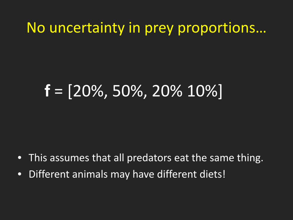
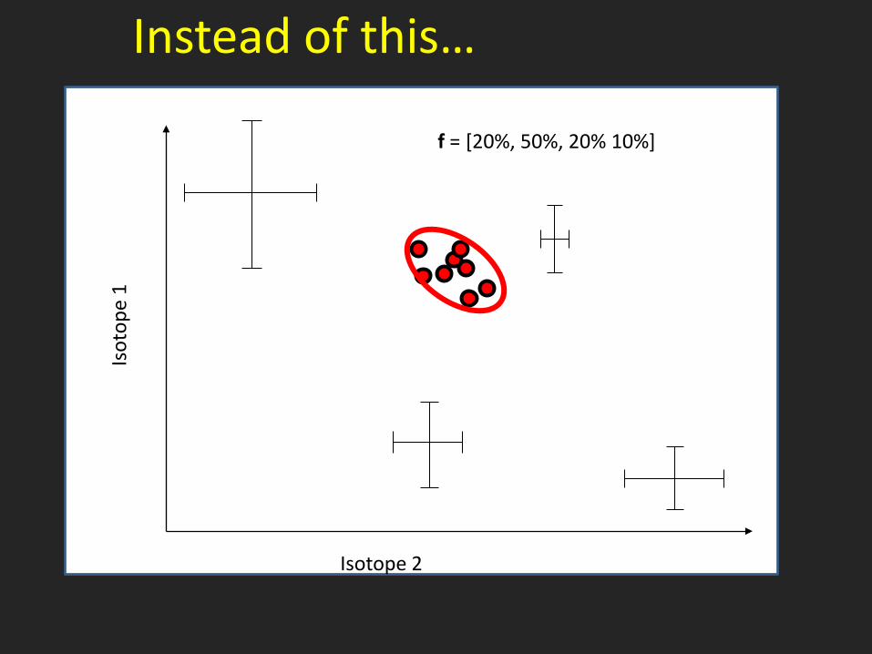
No uncertainty in prey proportions…
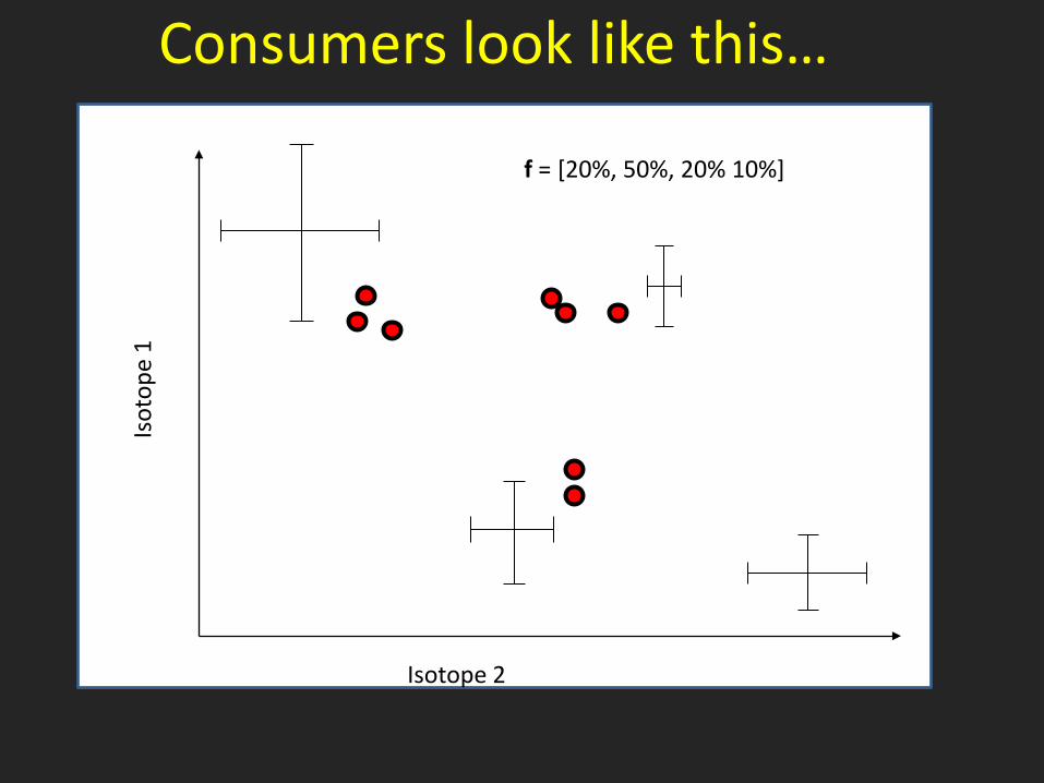
• This assumes that all predators eat the same thing.
• Different animals may have different diets!
f = [20%, 50%, 20% 10%]
Isot
ope
1
Isotope 2
Instead of this…
f = [20%, 50%, 20% 10%]
Isot
ope
1
Isotope 2
Consumers look like this…
f = [20%, 50%, 20% 10%]
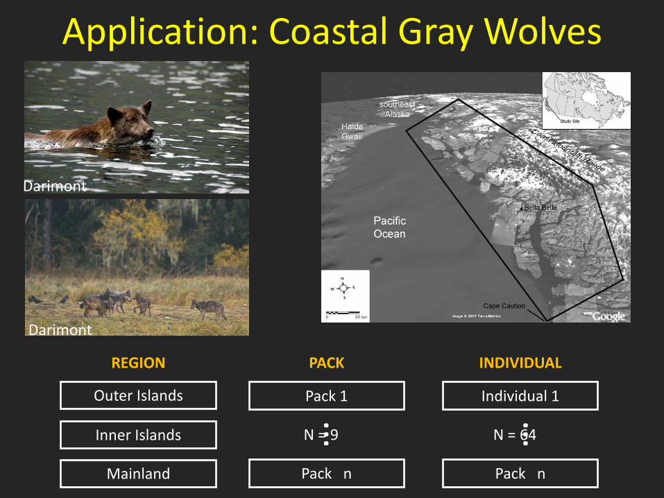
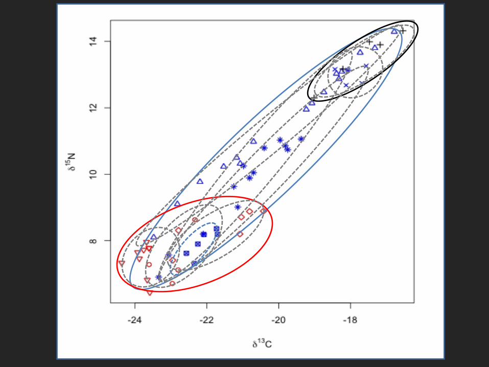
Application: Coastal Gray Wolves
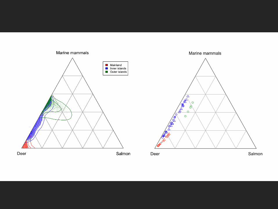
Outer Islands
Inner Islands
Mainland
Pack 1
Pack n
…
Individual 1
Pack n
… N = 9 N = 64
REGION PACK INDIVIDUAL
Darimont
Darimont
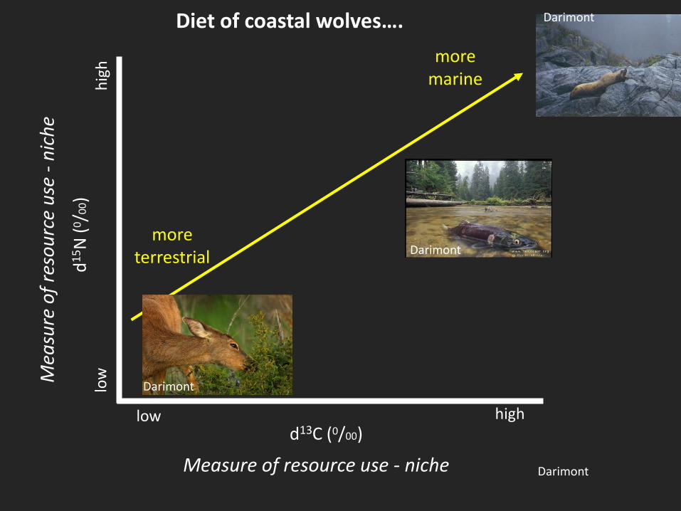
more terrestrial
more marine
d13C (0/00)
d15N
(0 /00
)
low high
low
hi
gh
Measure of resource use - niche
Mea
sure
of r
esou
rce
use
- nic
he
Diet of coastal wolves….
Darimont
Darimont
Darimont
Darimont
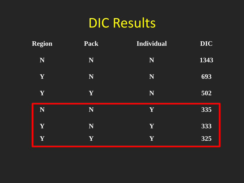
DIC Results Region Pack Individual DIC
N N N 1343
Y N N 693
Y Y N 502
N N Y 335
Y N Y 333
Y Y Y 325

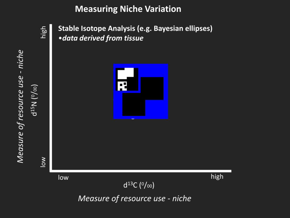
How to quantify niche?
• How variable is your isotopic signature?
• How variable are the resources you consume? – Dietary niche, we can output of the hierarchical
mixing model to get this
d13C (0/00)
d15N
(0 /00
)
low high
low
hi
gh
Measure of resource use - niche
Mea
sure
of r
esou
rce
use
- nic
he
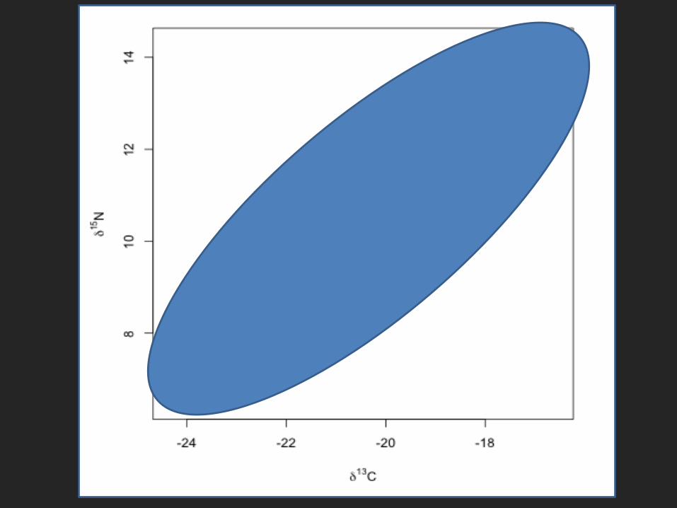
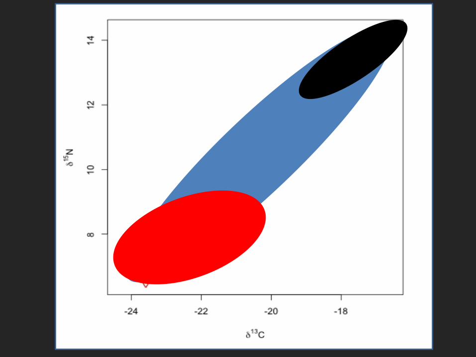
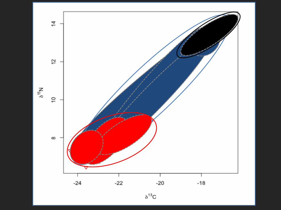
Stable Isotope Analysis (e.g. Bayesian ellipses) •data derived from tissue
Measuring Niche Variation
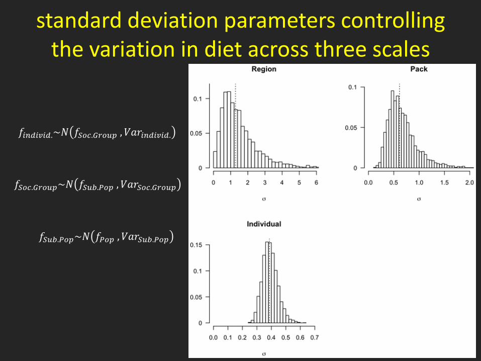
standard deviation parameters controlling the variation in diet across three scales
Other extensions to MixSIR
• Improving uncertainty in sources – Source signatures may be based on a small
number of samples
– We may have data from other systems to inform these
– In addition to treating the proportional contributions as parameters, the source means and variances also become parameters

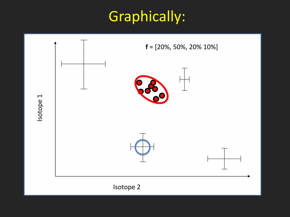
Dealing with source uncertainty
Ward, E.J., Semmens, B.X., and D.E. Schindler. 2010. Including source uncertainty and prior information in the analysis of stable isotope mixing models. Environmental Science & Technology, 44(12): 4645-4650
Figure 5: Map of Urban Lakes Gradient locations.
I Isot
ope
1
Isotope 2
Graphically:
f = [20%, 50%, 20% 10%]
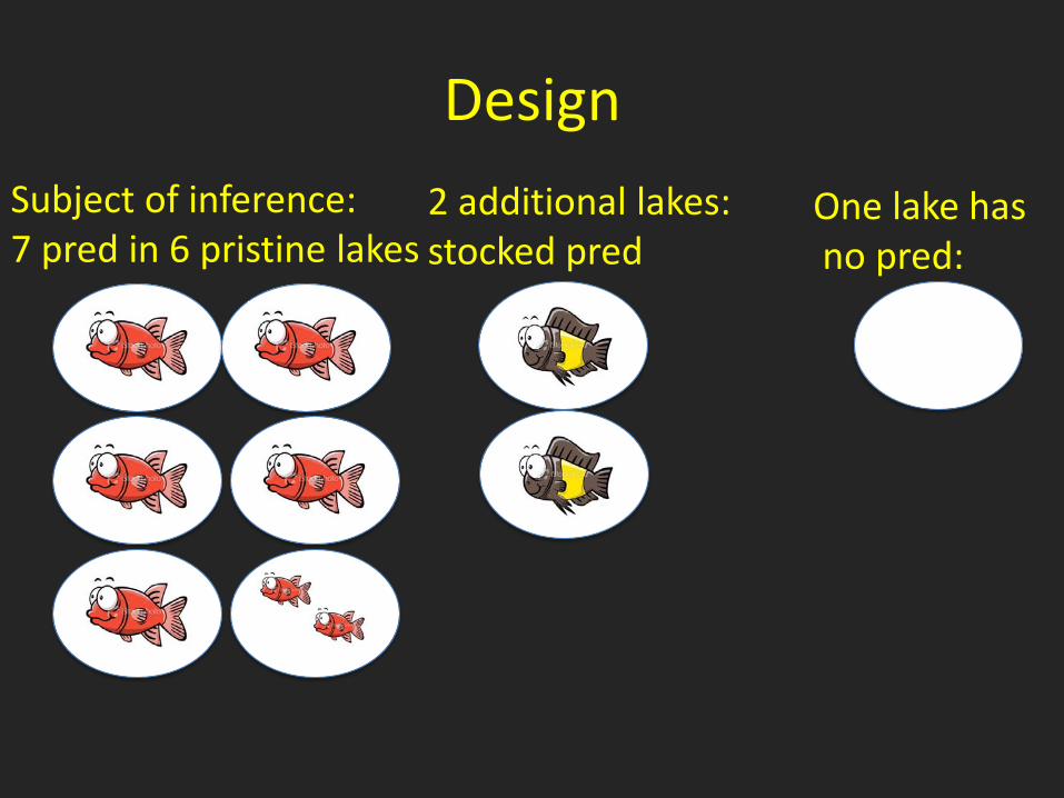
Design Subject of inference: 7 pred in 6 pristine lakes
One lake has no pred:
2 additional lakes: stocked pred
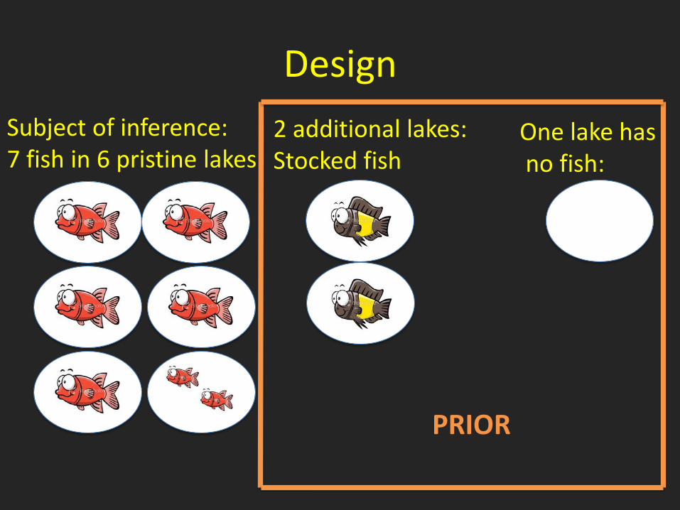
Design Subject of inference: 7 fish in 6 pristine lakes
One lake has no fish:
2 additional lakes: Stocked fish
PRIOR
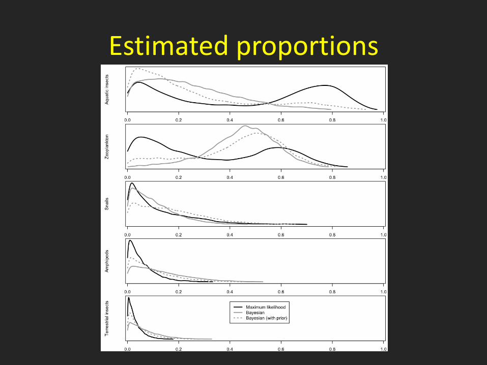
Estimated proportions
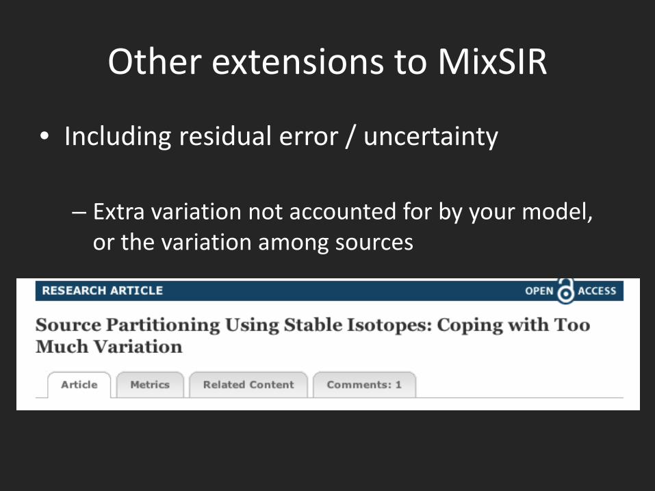
Other extensions to MixSIR
• Including residual error / uncertainty
– Extra variation not accounted for by your model, or the variation among sources
SIAR package in R
• Good if you don’t have identifying information about individuals (groups, etc)
• May help estimation if you’re missing a minor source
• Being fused with MixSIR = MixSIAR
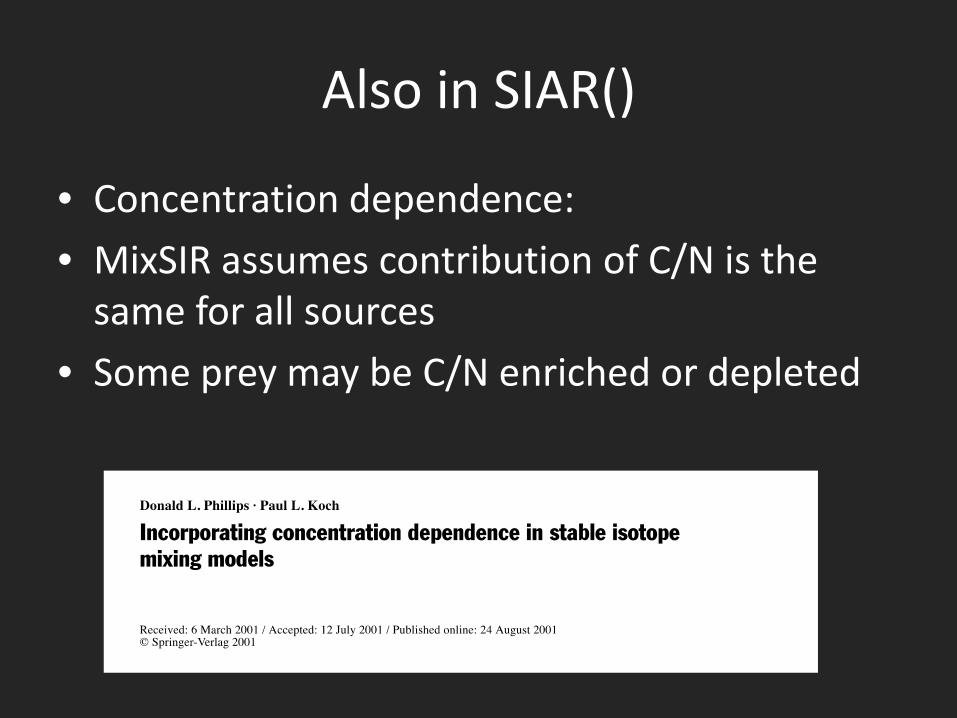
Also in SIAR()
• Concentration dependence:
• MixSIR assumes contribution of C/N is the same for all sources
• Some prey may be C/N enriched or depleted
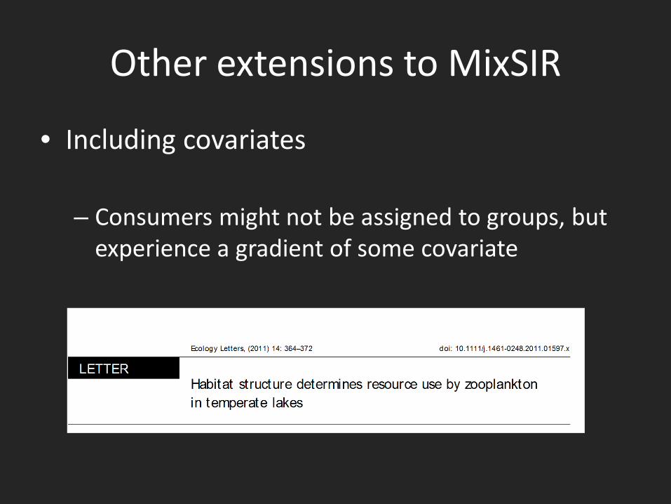
Other extensions to MixSIR
• Including covariates
– Consumers might not be assigned to groups, but experience a gradient of some covariate
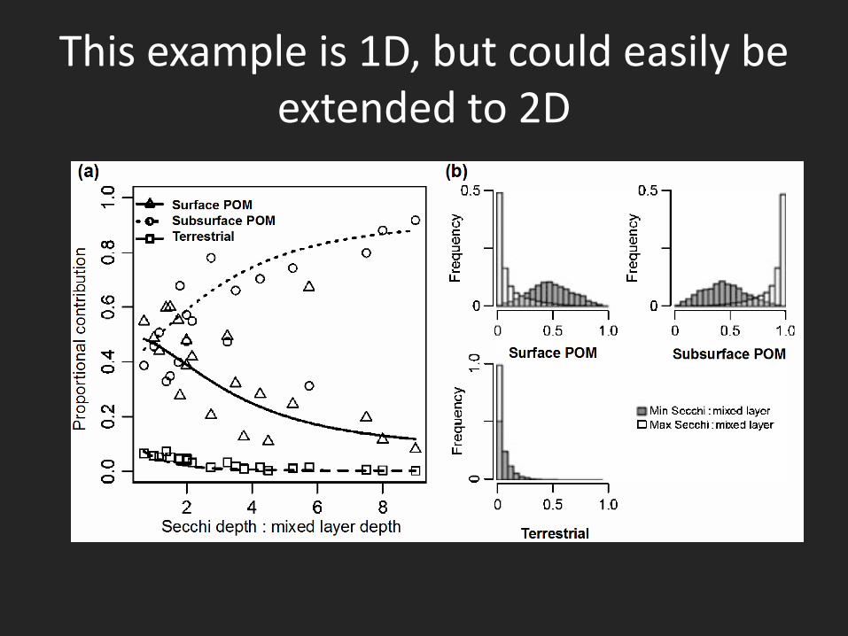
This example is 1D, but could easily be extended to 2D
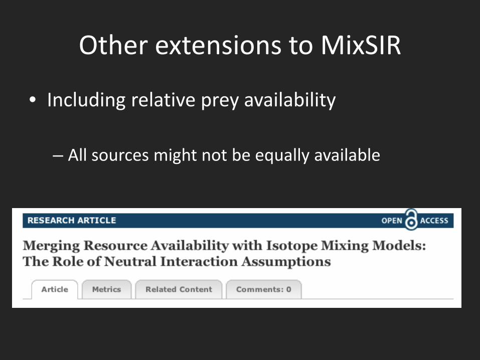
Other extensions to MixSIR
• Including relative prey availability
– All sources might not be equally available
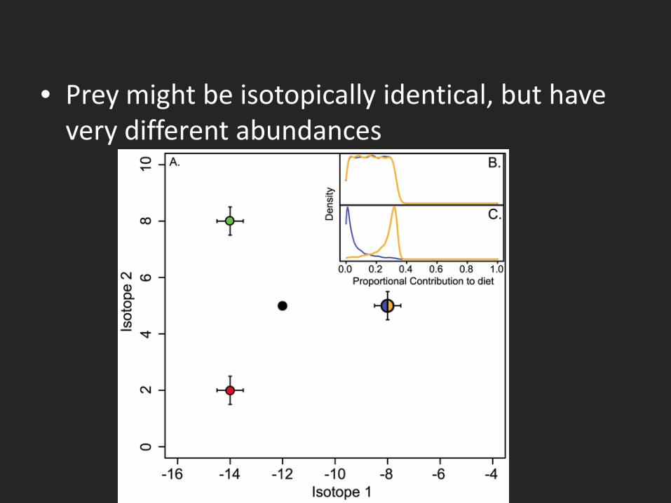
• Prey might be isotopically identical, but have very different abundances
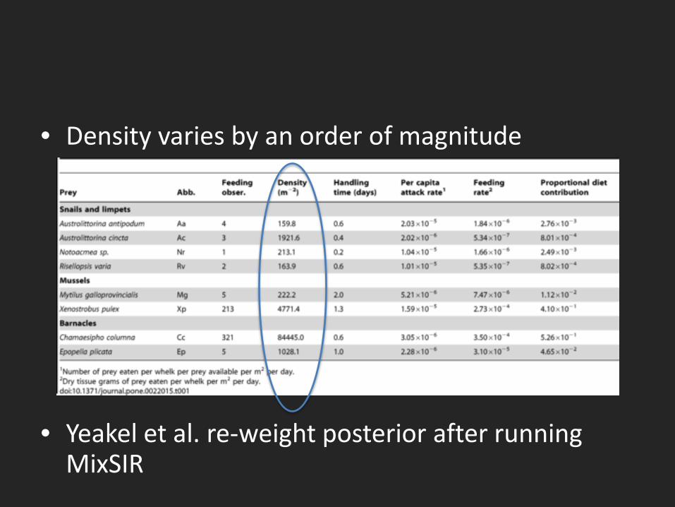
• Density varies by an order of magnitude
• Yeakel et al. re-weight posterior after running MixSIR
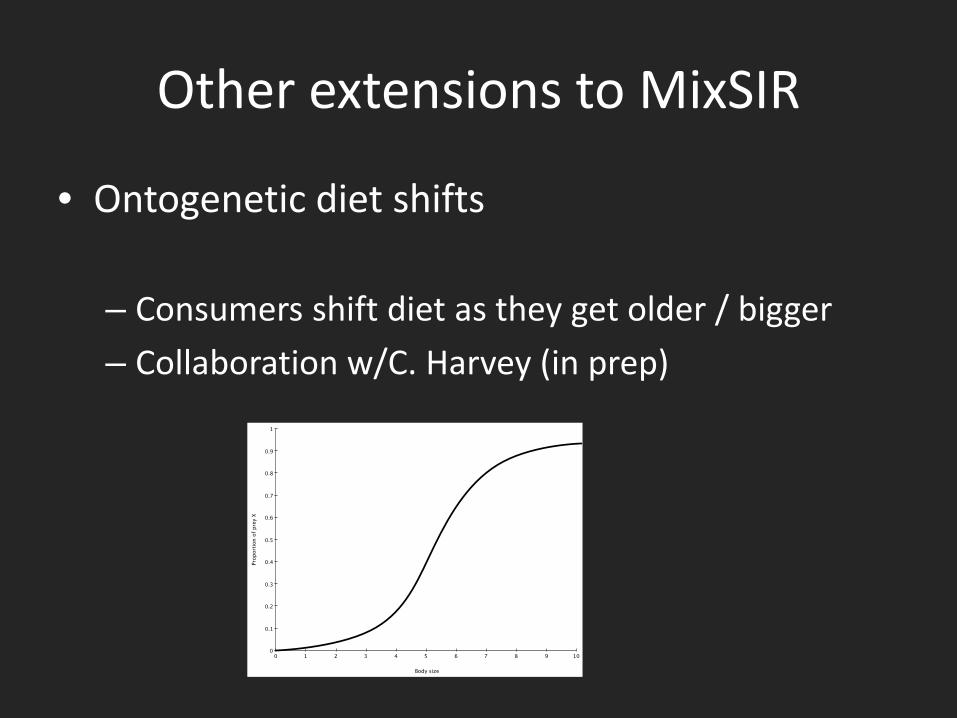
Other extensions to MixSIR
• Ontogenetic diet shifts
– Consumers shift diet as they get older / bigger
– Collaboration w/C. Harvey (in prep)
Other extensions to MixSIR
• Incorporating movement and the Isoscape
– Isotopic signatures of consumers reflect environment they inhabit
– We can infer where animals have been based on signatures
– Collaboration w/ J. Moore & C. Phillis
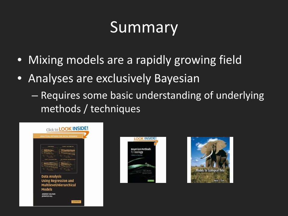
Summary
• Mixing models are a rapidly growing field
• Analyses are exclusively Bayesian – Requires some basic understanding of underlying
methods / techniques

Where Can I Get These Glorious Tools?
• http://www.ecologybox.org
• Tools include: – R code to run
– Worked examples
– Step-by-step code explanations

isoecol.blogspot.com
Acknowledgements
NOAA Seattle • Brice Semmens • Eli Holmes • Mark Scheuerell • Eric Buhle • Tessa Francis UC Santa Cruz • Jon Moore • Chris Darimont UW • Daniel Schindler • Gordon Holtgrieve • Tessa Francis
• Additional collaborators • Andrew Jackson • Stu Bearhop • Andrew Parnell • Rich Inger • Don Phillips
Recommended


![Medical Isotope Production and Use [March 2009] - National Isotope](https://img.pdfslide.us/doc/110x75/62038cd4da24ad121e4ab7b4/medical-isotope-production-and-use-march-2009-national-isotope.jpg)