Introduction to Algorithms6.046J/18.401J/SMA5503
Lecture 1Prof. Charles E. Leiserson
Day 1 Introduction to Algorithms L1.2
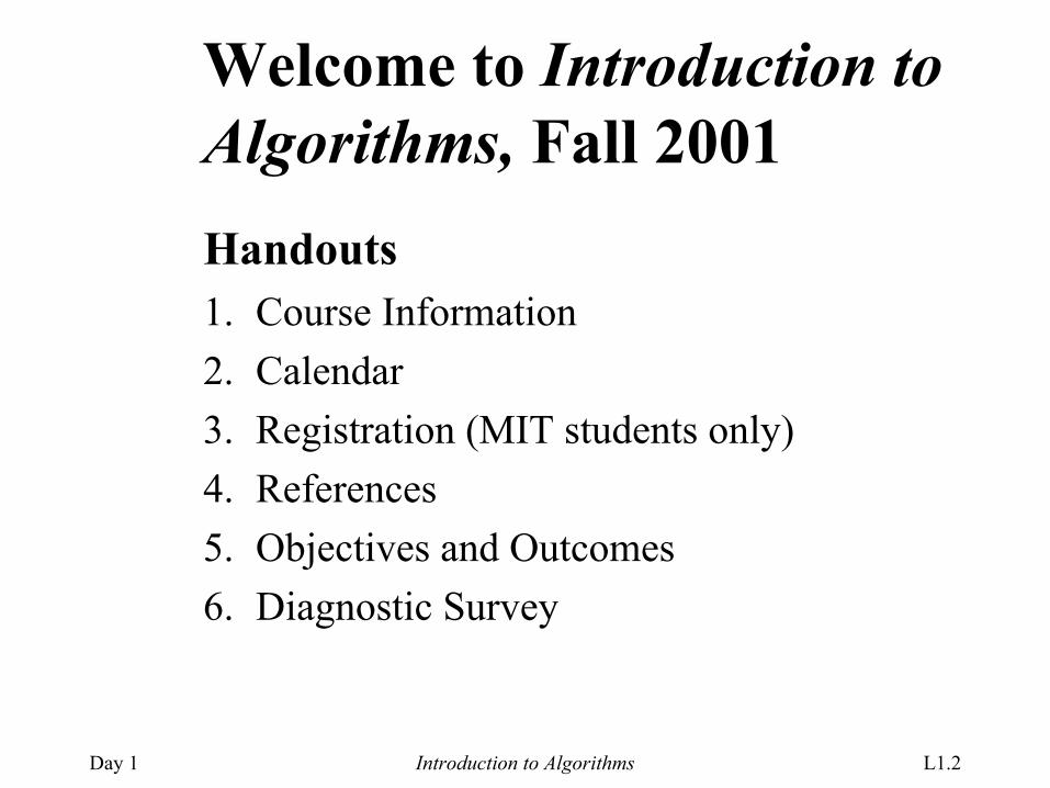
Welcome to Introduction to Algorithms, Fall 2001Handouts1. Course Information2. Calendar3. Registration (MIT students only)4. References5. Objectives and Outcomes6. Diagnostic Survey
Day 1 Introduction to Algorithms L1.3
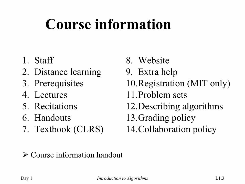
Course information
1. Staff2. Distance learning3. Prerequisites4. Lectures5. Recitations6. Handouts7. Textbook (CLRS)
8. Website9. Extra help10.Registration (MIT only)11.Problem sets12.Describing algorithms13.Grading policy14.Collaboration policy
Course information handout
Day 1 Introduction to Algorithms L1.4
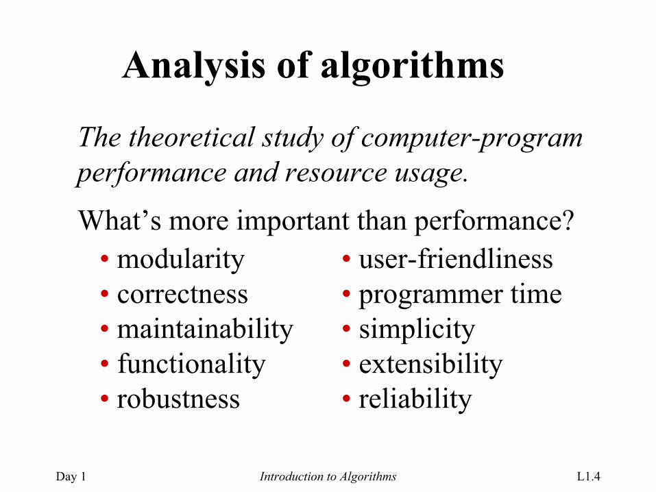
Analysis of algorithms
The theoretical study of computer-program performance and resource usage.
What’s more important than performance?• modularity• correctness• maintainability• functionality• robustness
• user-friendliness• programmer time• simplicity• extensibility• reliability

Day 1 Introduction to Algorithms L1.5
Why study algorithms and performance?
• Algorithms help us to understand scalability.• Performance often draws the line between what
is feasible and what is impossible.• Algorithmic mathematics provides a language
for talking about program behavior.• The lessons of program performance generalize
to other computing resources. • Speed is fun!
Day 1 Introduction to Algorithms L1.6
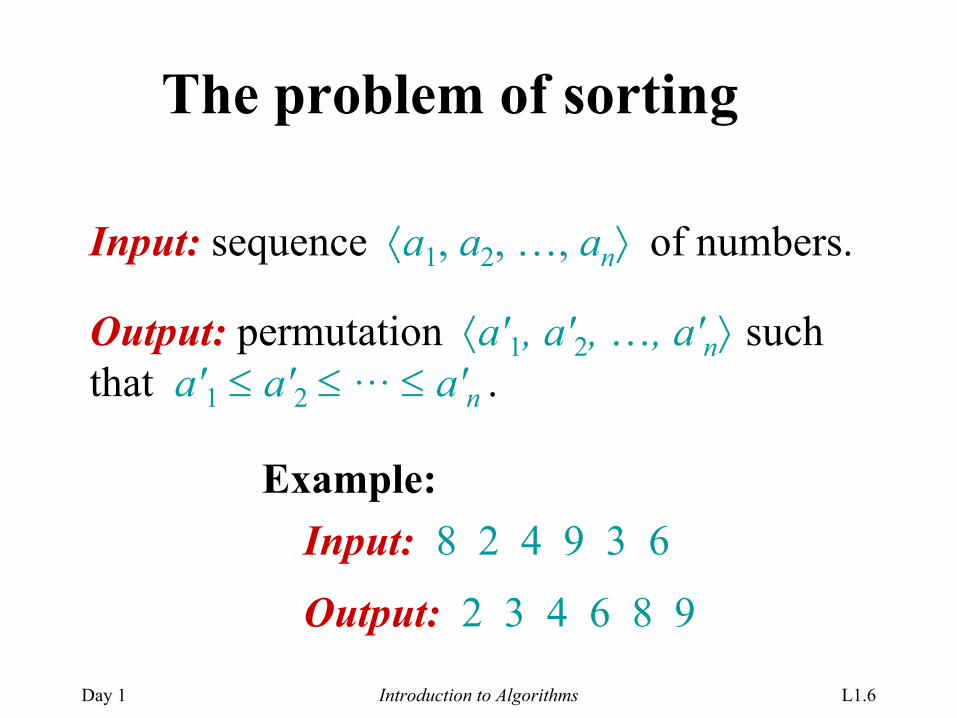
The problem of sorting
Input: sequence ⟨a1, a2, …, an⟩ of numbers.
Example:Input: 8 2 4 9 3 6
Output: 2 3 4 6 8 9
Output: permutation ⟨a'1, a'2, …, a'n⟩ suchthat a'1 ≤ a'2 ≤ … ≤ a'n .
Day 1 Introduction to Algorithms L1.7
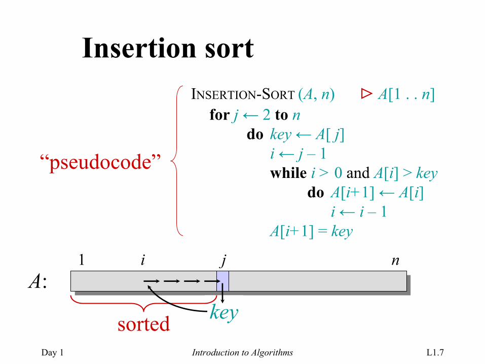
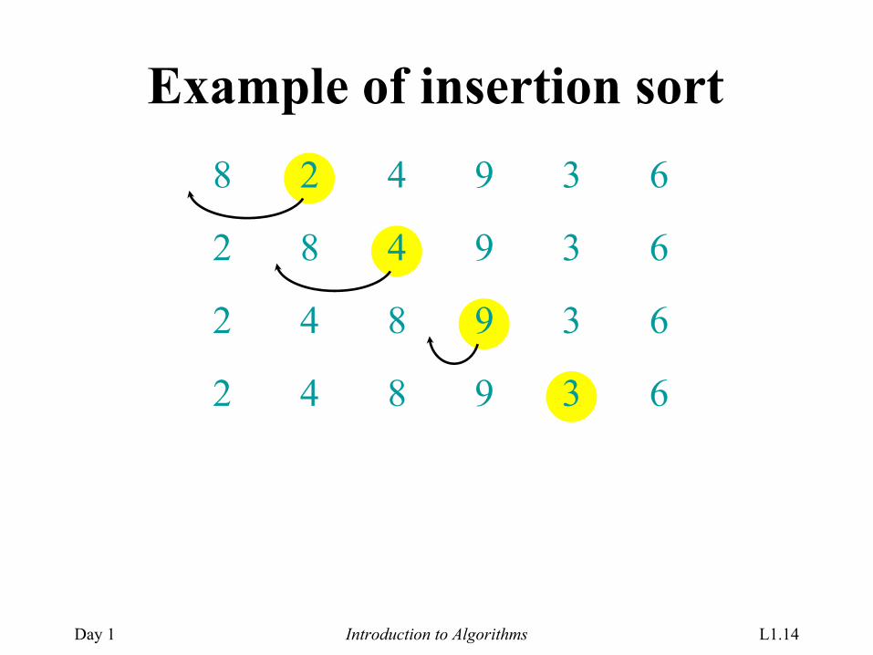
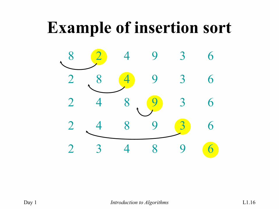
Insertion sortINSERTION-SORT (A, n) ⊳ A[1 . . n]
for j ← 2 to ndo key ← A[ j]
i ← j – 1while i > 0 and A[i] > key
do A[i+1] ← A[i]i ← i – 1
A[i+1] = key
“pseudocode”
i j
keysorted
A:1 n
Day 1 Introduction to Algorithms L1.8
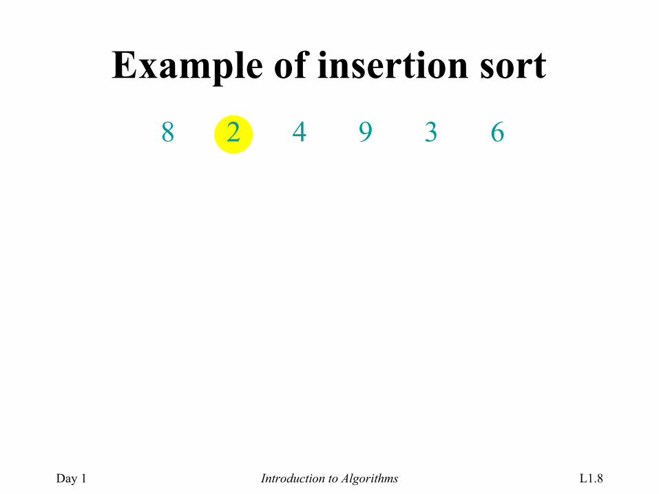
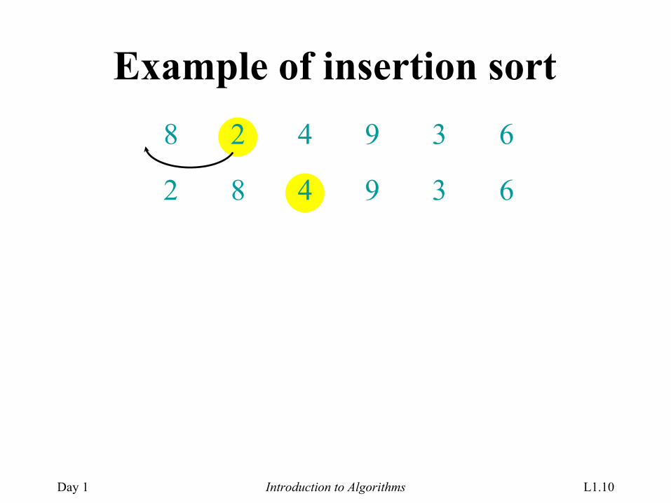
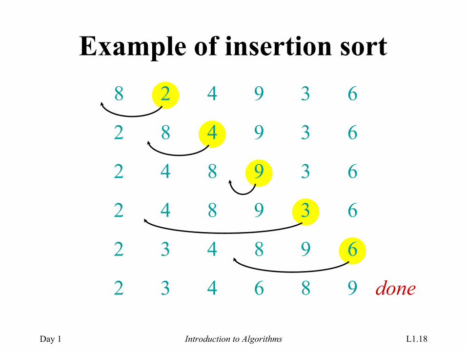
Example of insertion sort8 2 4 9 3 6
Day 1 Introduction to Algorithms L1.9
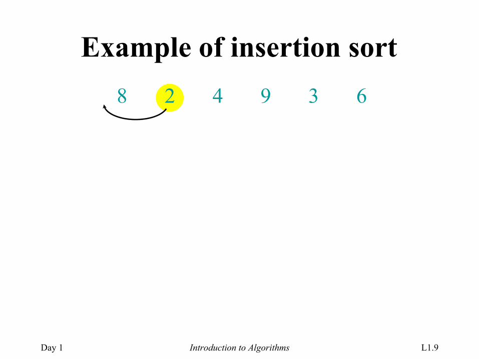
Example of insertion sort8 2 4 9 3 6
Day 1 Introduction to Algorithms L1.10
Example of insertion sort8 2 4 9 3 6
2 8 4 9 3 6
Day 1 Introduction to Algorithms L1.11
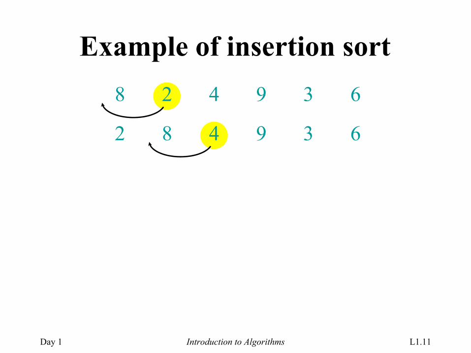
Example of insertion sort8 2 4 9 3 6
2 8 4 9 3 6
Day 1 Introduction to Algorithms L1.12
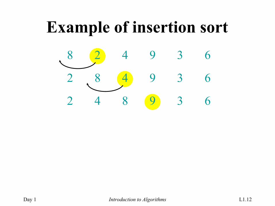
Example of insertion sort8 2 4 9 3 6
2 8 4 9 3 6
2 4 8 9 3 6
Day 1 Introduction to Algorithms L1.13
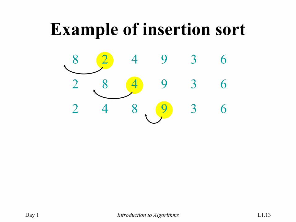
Example of insertion sort8 2 4 9 3 6
2 8 4 9 3 6
2 4 8 9 3 6
Day 1 Introduction to Algorithms L1.14
Example of insertion sort8 2 4 9 3 6
2 8 4 9 3 6
2 4 8 9 3 6
2 4 8 9 3 6
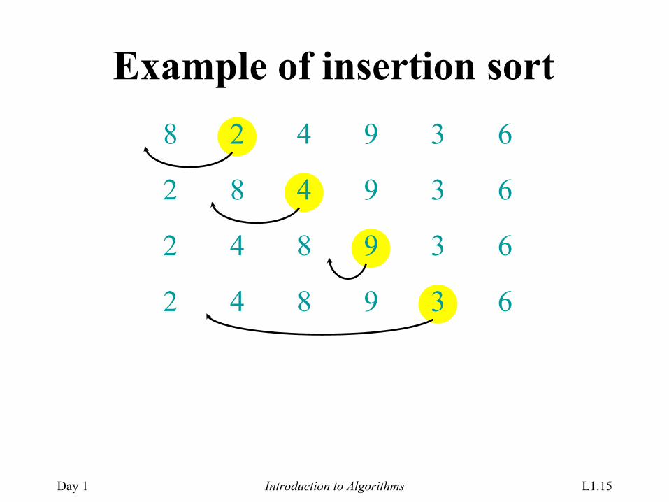
Day 1 Introduction to Algorithms L1.15
Example of insertion sort8 2 4 9 3 6
2 8 4 9 3 6
2 4 8 9 3 6
2 4 8 9 3 6
Day 1 Introduction to Algorithms L1.16
Example of insertion sort8 2 4 9 3 6
2 8 4 9 3 6
2 4 8 9 3 6
2 4 8 9 3 6
2 3 4 8 9 6
Day 1 Introduction to Algorithms L1.17
Example of insertion sort8 2 4 9 3 6
2 8 4 9 3 6
2 4 8 9 3 6
2 4 8 9 3 6
2 3 4 8 9 6
Day 1 Introduction to Algorithms L1.18
Example of insertion sort8 2 4 9 3 6
2 8 4 9 3 6
2 4 8 9 3 6
2 4 8 9 3 6
2 3 4 8 9 6
2 3 4 6 8 9 done
Day 1 Introduction to Algorithms L1.19
Running time
• The running time depends on the input: an already sorted sequence is easier to sort.
• Parameterize the running time by the size of the input, since short sequences are easier to sort than long ones.
• Generally, we seek upper bounds on the running time, because everybody likes a guarantee.
Day 1 Introduction to Algorithms L1.20
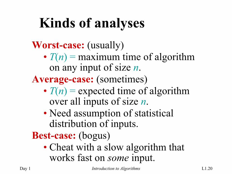
Kinds of analysesWorst-case: (usually)
• T(n) = maximum time of algorithm on any input of size n.
Average-case: (sometimes)• T(n) = expected time of algorithm
over all inputs of size n.• Need assumption of statistical
distribution of inputs.Best-case: (bogus)
• Cheat with a slow algorithm that works fast on some input.
Day 1 Introduction to Algorithms L1.21
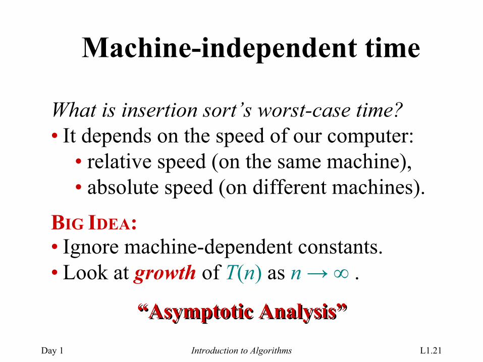
Machine-independent time
What is insertion sort’s worst-case time?• It depends on the speed of our computer:
• relative speed (on the same machine),• absolute speed (on different machines).
BIG IDEA:• Ignore machine-dependent constants.• Look at growth of T(n) as n →∞ .
“Asymptotic Analysis”“Asymptotic Analysis”
Day 1 Introduction to Algorithms L1.22
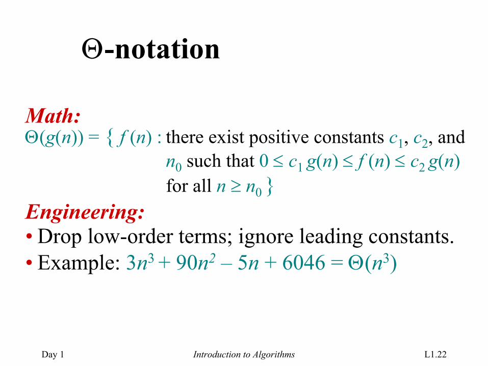
Θ-notation
• Drop low-order terms; ignore leading constants.• Example: 3n3 + 90n2 – 5n + 6046 = Θ(n3)
Math:Θ(g(n)) = { f (n) : there exist positive constants c1, c2, and
n0 such that 0 ≤ c1 g(n) ≤ f (n) ≤ c2 g(n)for all n ≥ n0 }
Engineering:
Day 1 Introduction to Algorithms L1.23
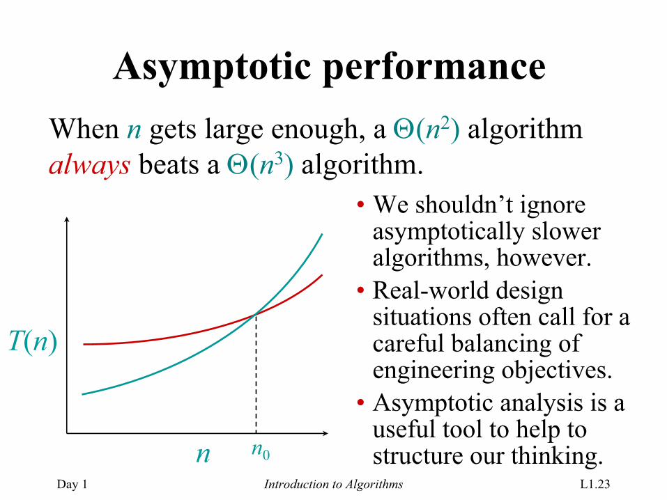
Asymptotic performance
n
T(n)
n0
• We shouldn’t ignore asymptotically slower algorithms, however.
• Real-world design situations often call for a careful balancing of engineering objectives.
• Asymptotic analysis is a useful tool to help to structure our thinking.
When n gets large enough, a Θ(n2) algorithm always beats a Θ(n3) algorithm.
Day 1 Introduction to Algorithms L1.24
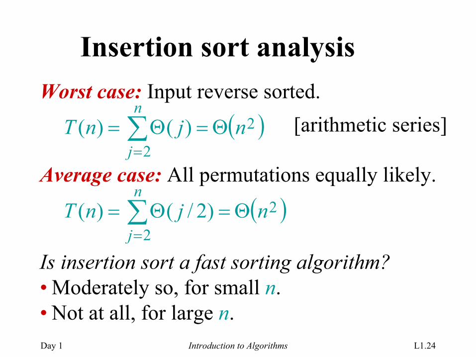
Insertion sort analysisWorst case: Input reverse sorted.
( )∑=
Θ=Θ=n
jnjnT
2
2)()(
Average case: All permutations equally likely.
( )∑=
Θ=Θ=n
jnjnT
2
2)2/()(
Is insertion sort a fast sorting algorithm?• Moderately so, for small n.• Not at all, for large n.
[arithmetic series]
Day 1 Introduction to Algorithms L1.25
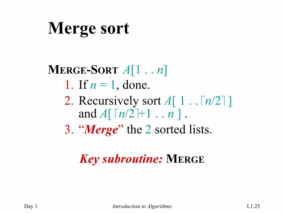
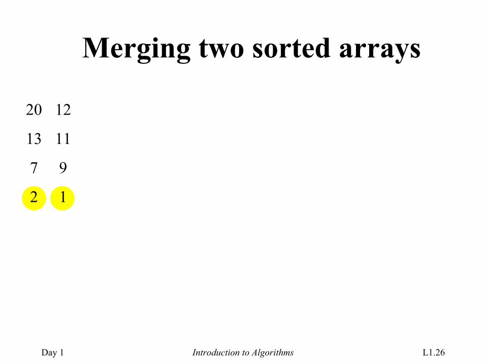
Merge sort
MERGE-SORT A[1 . . n]1. If n = 1, done.2. Recursively sort A[ 1 . . n/2 ]
and A[ n/2+1 . . n ] .3. “Merge” the 2 sorted lists.
Key subroutine: MERGE
Day 1 Introduction to Algorithms L1.26
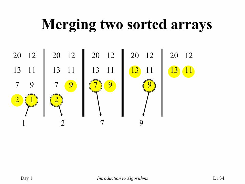
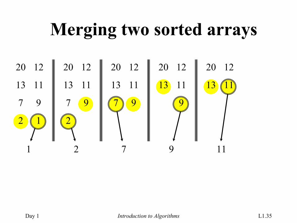
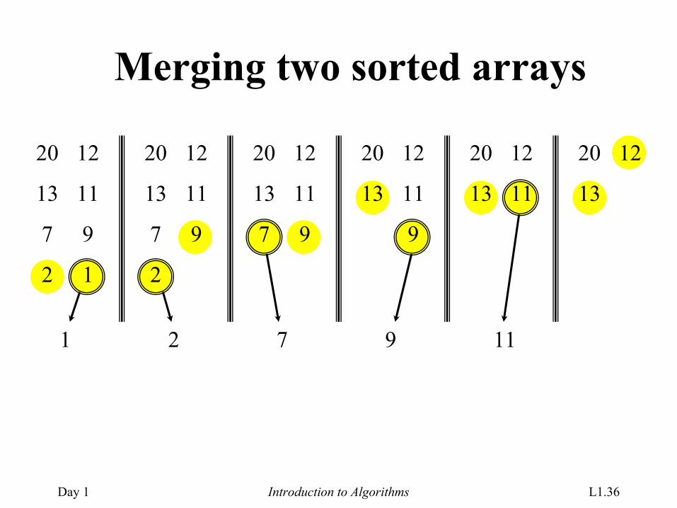
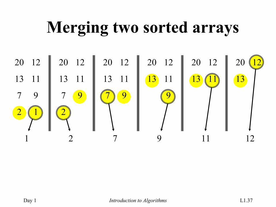
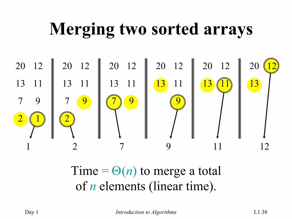
Merging two sorted arrays
20
13
7
2
12
11
9
1
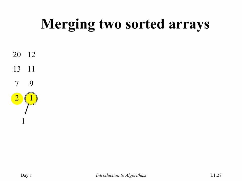
Day 1 Introduction to Algorithms L1.27
Merging two sorted arrays
20
13
7
2
12
11
9
1
1
Day 1 Introduction to Algorithms L1.28
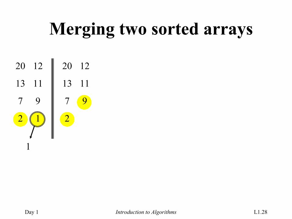
Merging two sorted arrays
20
13
7
2
12
11
9
1
1
20
13
7
2
12
11
9
Day 1 Introduction to Algorithms L1.29
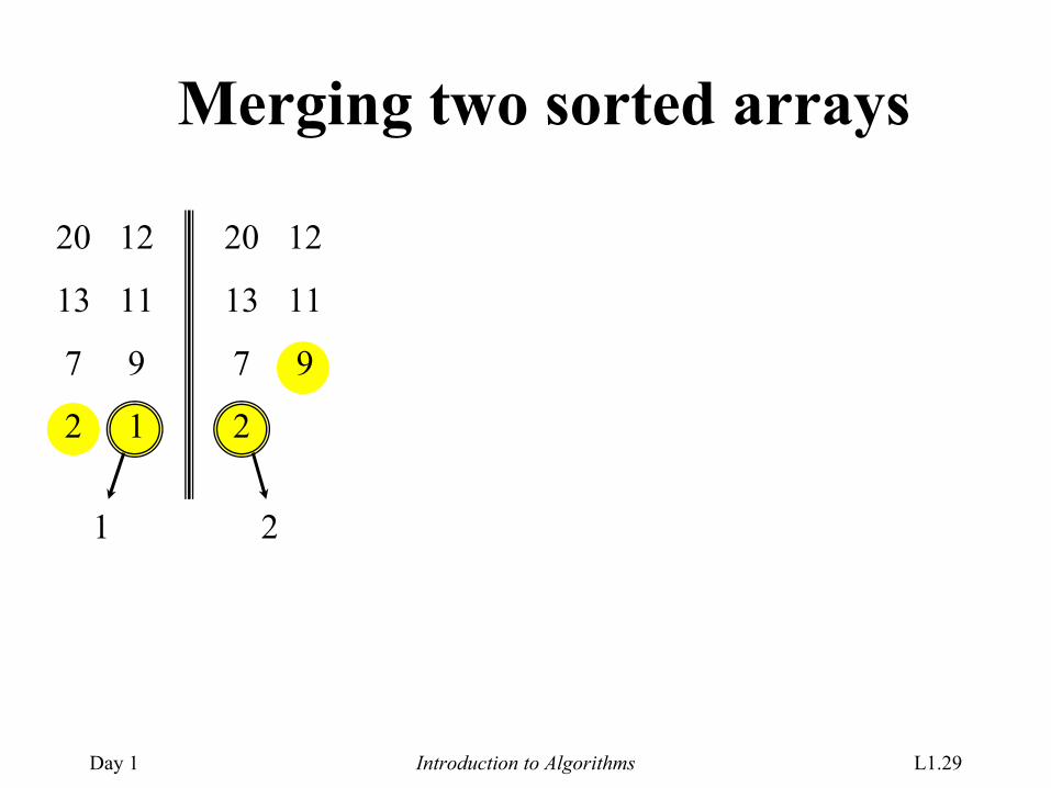
Merging two sorted arrays
20
13
7
2
12
11
9
1
1
20
13
7
2
12
11
9
2
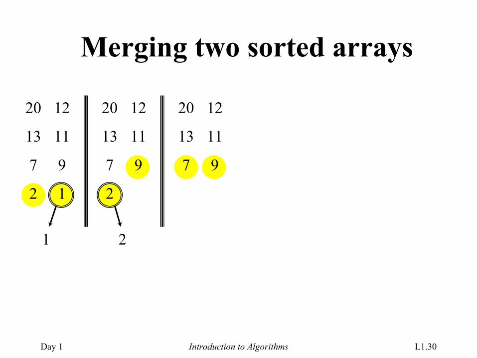
Day 1 Introduction to Algorithms L1.30
Merging two sorted arrays
20
13
7
2
12
11
9
1
1
20
13
7
2
12
11
9
2
20
13
7
12
11
9
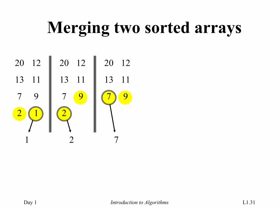
Day 1 Introduction to Algorithms L1.31
Merging two sorted arrays
20
13
7
2
12
11
9
1
1
20
13
7
2
12
11
9
2
20
13
7
12
11
9
7
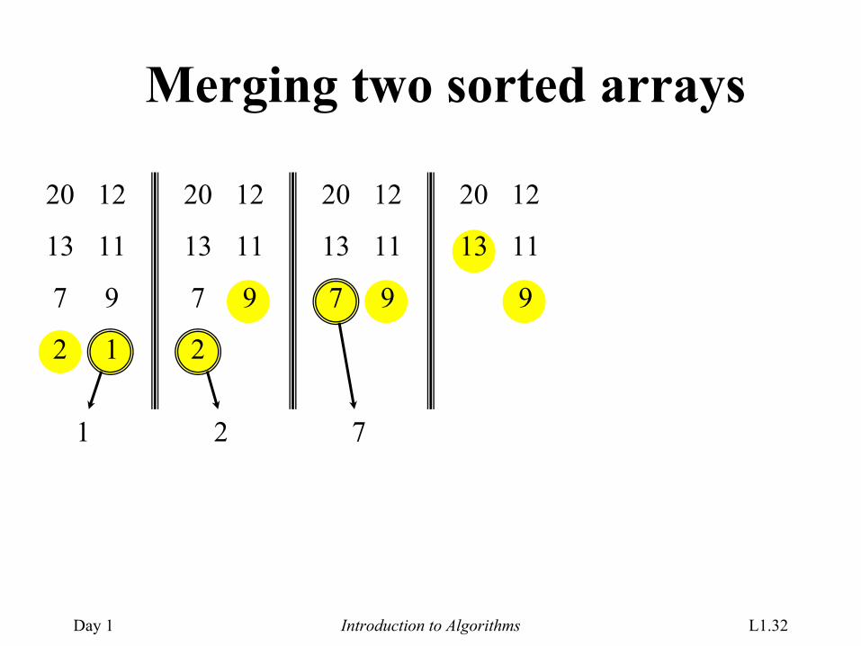
Day 1 Introduction to Algorithms L1.32
Merging two sorted arrays
20
13
7
2
12
11
9
1
1
20
13
7
2
12
11
9
2
20
13
7
12
11
9
7
20
13
12
11
9
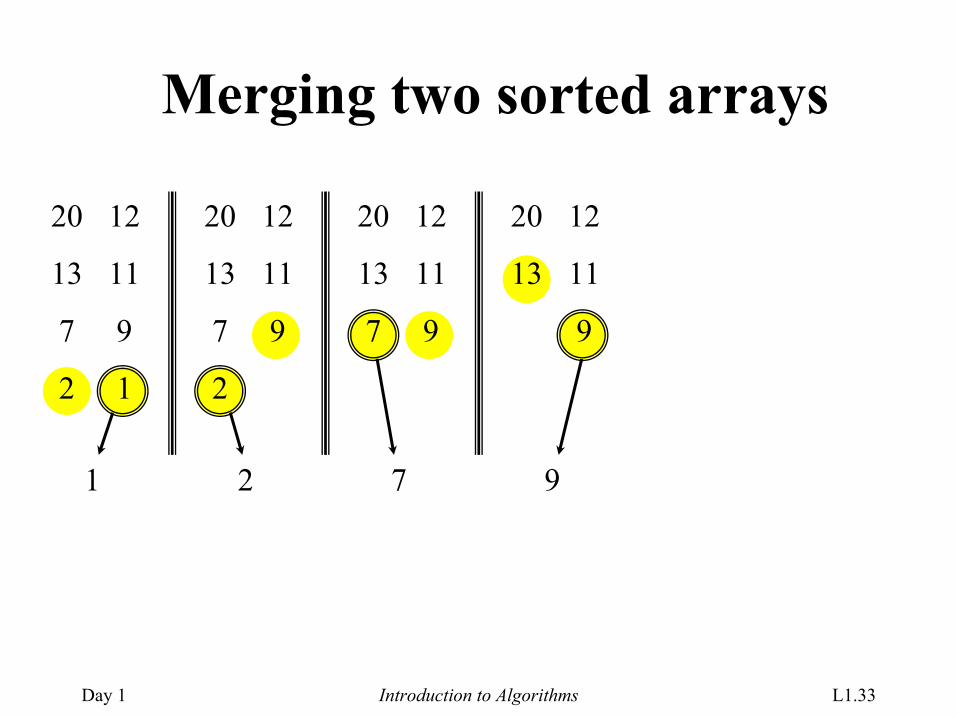
Day 1 Introduction to Algorithms L1.33
Merging two sorted arrays
20
13
7
2
12
11
9
1
1
20
13
7
2
12
11
9
2
20
13
7
12
11
9
7
20
13
12
11
9
9
Day 1 Introduction to Algorithms L1.34
Merging two sorted arrays
20
13
7
2
12
11
9
1
1
20
13
7
2
12
11
9
2
20
13
7
12
11
9
7
20
13
12
11
9
9
20
13
12
11
Day 1 Introduction to Algorithms L1.35
Merging two sorted arrays
20
13
7
2
12
11
9
1
1
20
13
7
2
12
11
9
2
20
13
7
12
11
9
7
20
13
12
11
9
9
20
13
12
11
11
Day 1 Introduction to Algorithms L1.36
Merging two sorted arrays
20
13
7
2
12
11
9
1
1
20
13
7
2
12
11
9
2
20
13
7
12
11
9
7
20
13
12
11
9
9
20
13
12
11
11
20
13
12
Day 1 Introduction to Algorithms L1.37
Merging two sorted arrays
20
13
7
2
12
11
9
1
1
20
13
7
2
12
11
9
2
20
13
7
12
11
9
7
20
13
12
11
9
9
20
13
12
11
11
20
13
12
12
Day 1 Introduction to Algorithms L1.38
Merging two sorted arrays
20
13
7
2
12
11
9
1
1
20
13
7
2
12
11
9
2
20
13
7
12
11
9
7
20
13
12
11
9
9
20
13
12
11
11
20
13
12
12
Time = Θ(n) to merge a total of n elements (linear time).
Day 1 Introduction to Algorithms L1.39
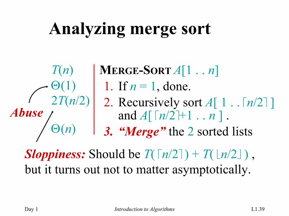
Analyzing merge sort
MERGE-SORT A[1 . . n]1. If n = 1, done.2. Recursively sort A[ 1 . . n/2 ]
and A[ n/2+1 . . n ] .3. “Merge” the 2 sorted lists
T(n)Θ(1)2T(n/2)
Θ(n)Abuse
Sloppiness: Should be T( n/2 ) + T( n/2 ) , but it turns out not to matter asymptotically.
Day 1 Introduction to Algorithms L1.40
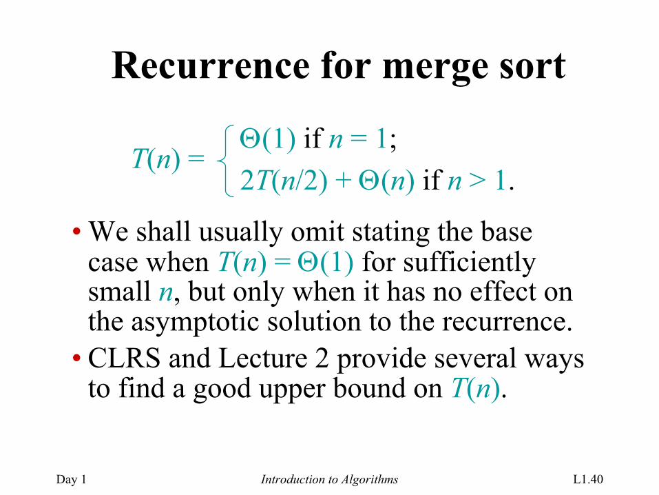
Recurrence for merge sort
T(n) =Θ(1) if n = 1;2T(n/2) + Θ(n) if n > 1.
• We shall usually omit stating the base case when T(n) = Θ(1) for sufficiently small n, but only when it has no effect on the asymptotic solution to the recurrence.
• CLRS and Lecture 2 provide several ways to find a good upper bound on T(n).
Day 1 Introduction to Algorithms L1.41
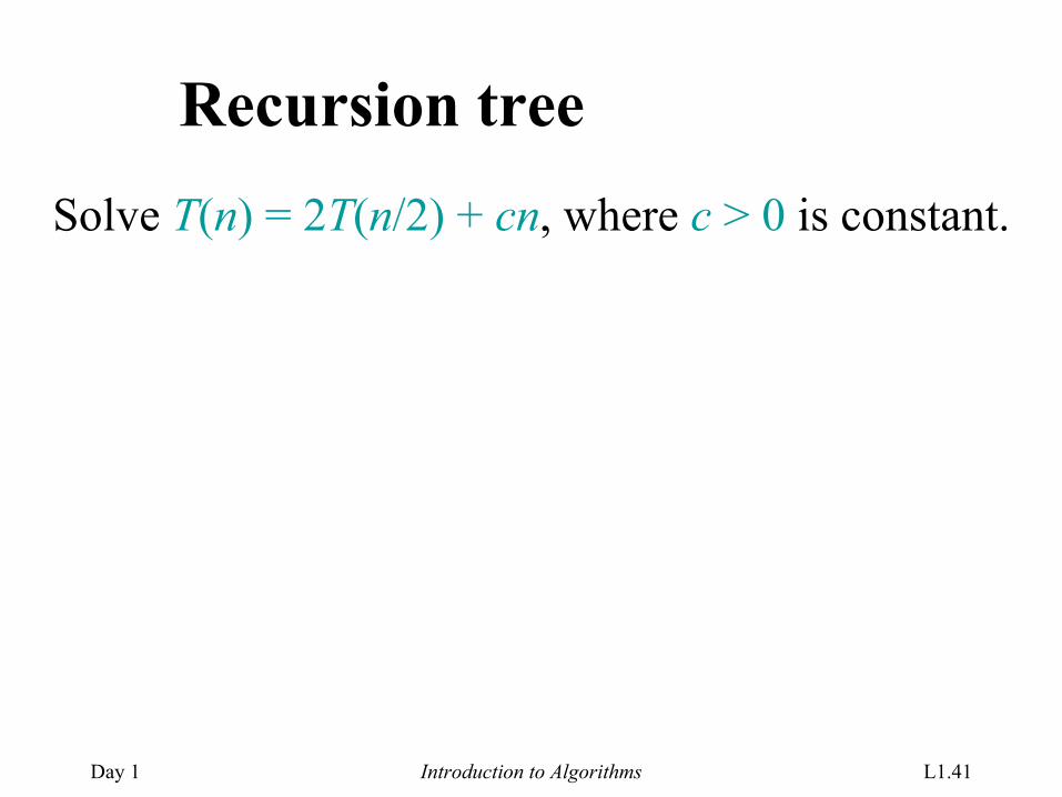
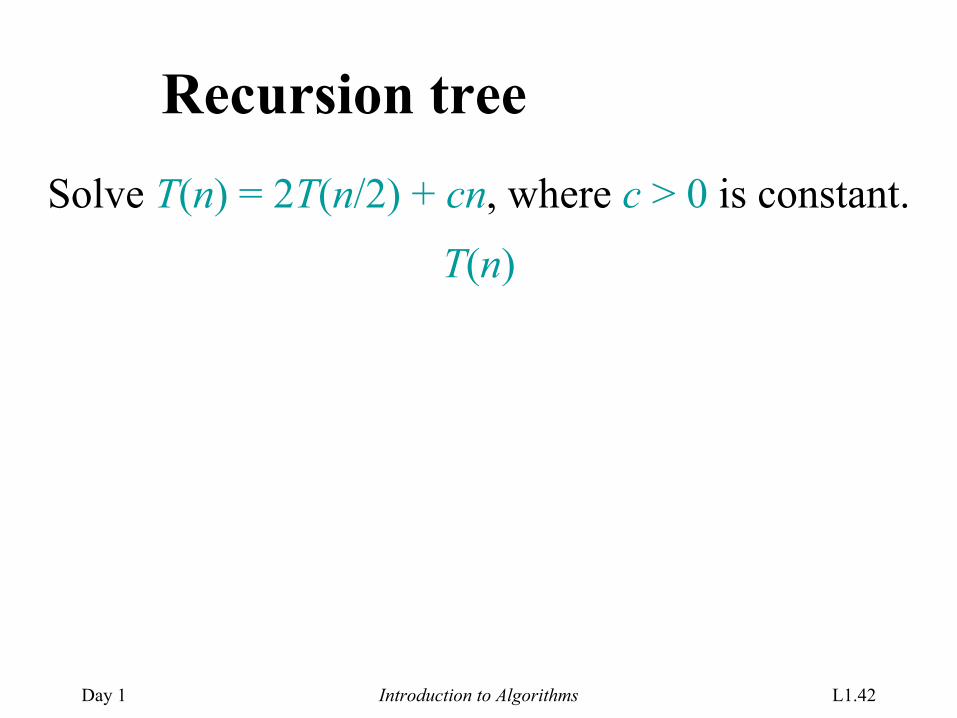
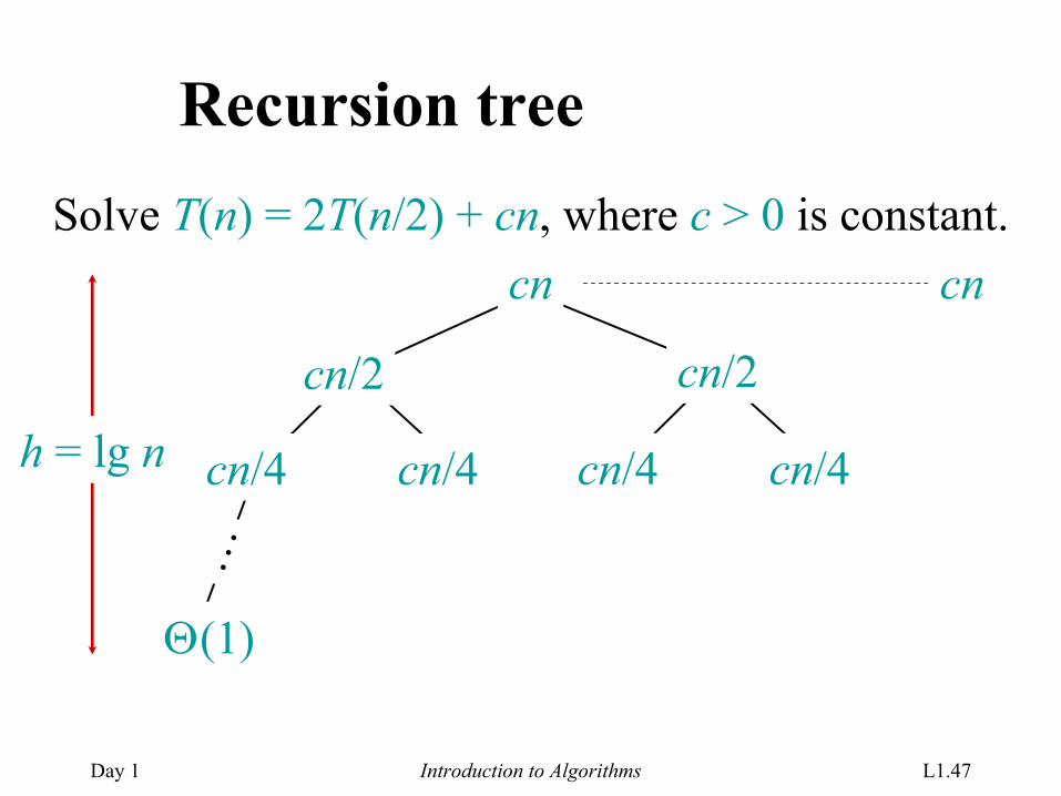
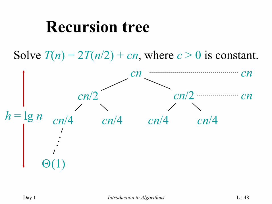
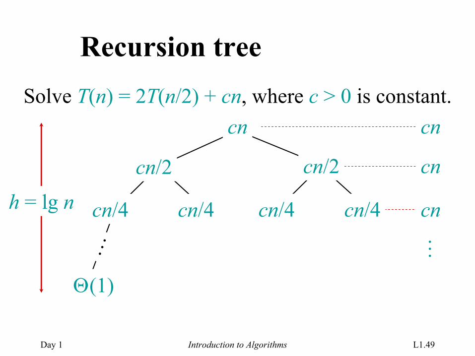
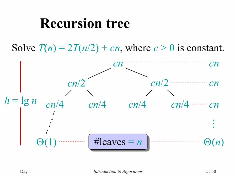
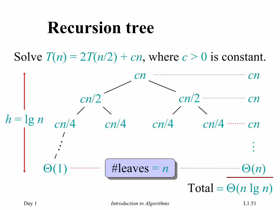
Recursion treeSolve T(n) = 2T(n/2) + cn, where c > 0 is constant.
Day 1 Introduction to Algorithms L1.42
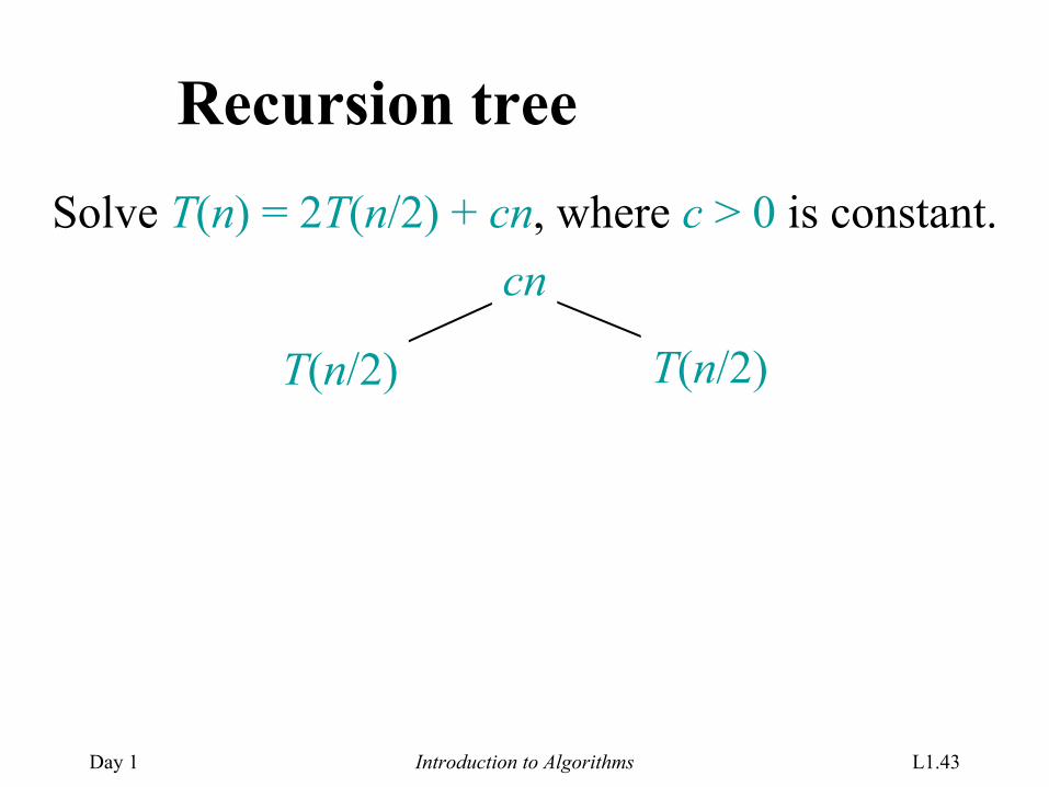
Recursion treeSolve T(n) = 2T(n/2) + cn, where c > 0 is constant.
T(n)
Day 1 Introduction to Algorithms L1.43
Recursion treeSolve T(n) = 2T(n/2) + cn, where c > 0 is constant.
T(n/2) T(n/2)
cn
Day 1 Introduction to Algorithms L1.44
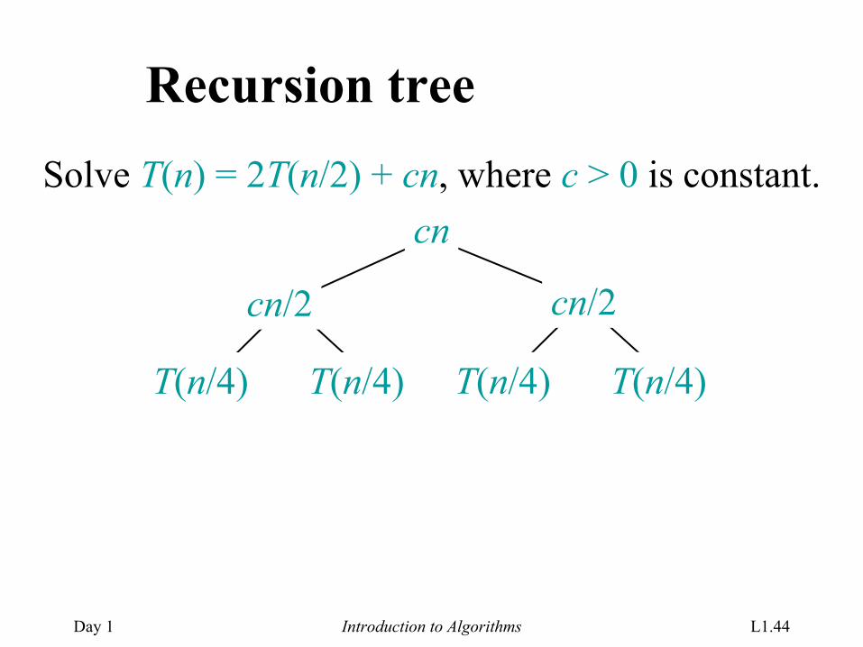
Recursion treeSolve T(n) = 2T(n/2) + cn, where c > 0 is constant.
cn
T(n/4) T(n/4) T(n/4) T(n/4)
cn/2 cn/2
Day 1 Introduction to Algorithms L1.45
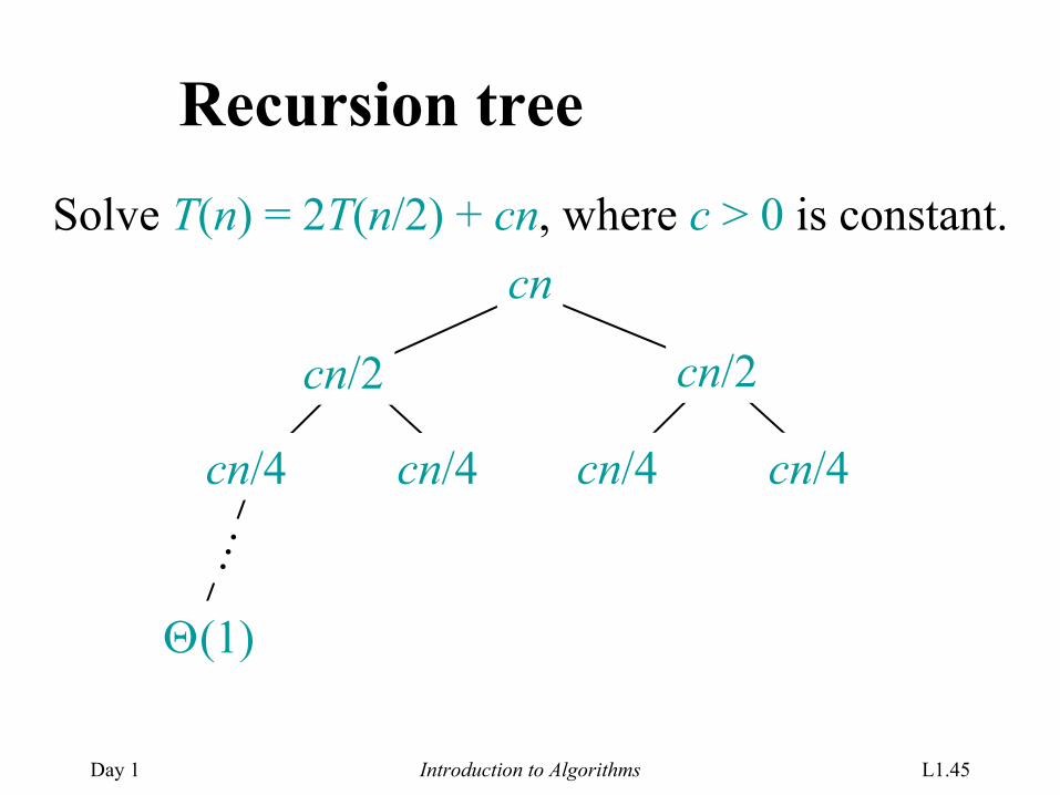
Recursion treeSolve T(n) = 2T(n/2) + cn, where c > 0 is constant.
cn
cn/4 cn/4 cn/4 cn/4
cn/2 cn/2
Θ(1)
…
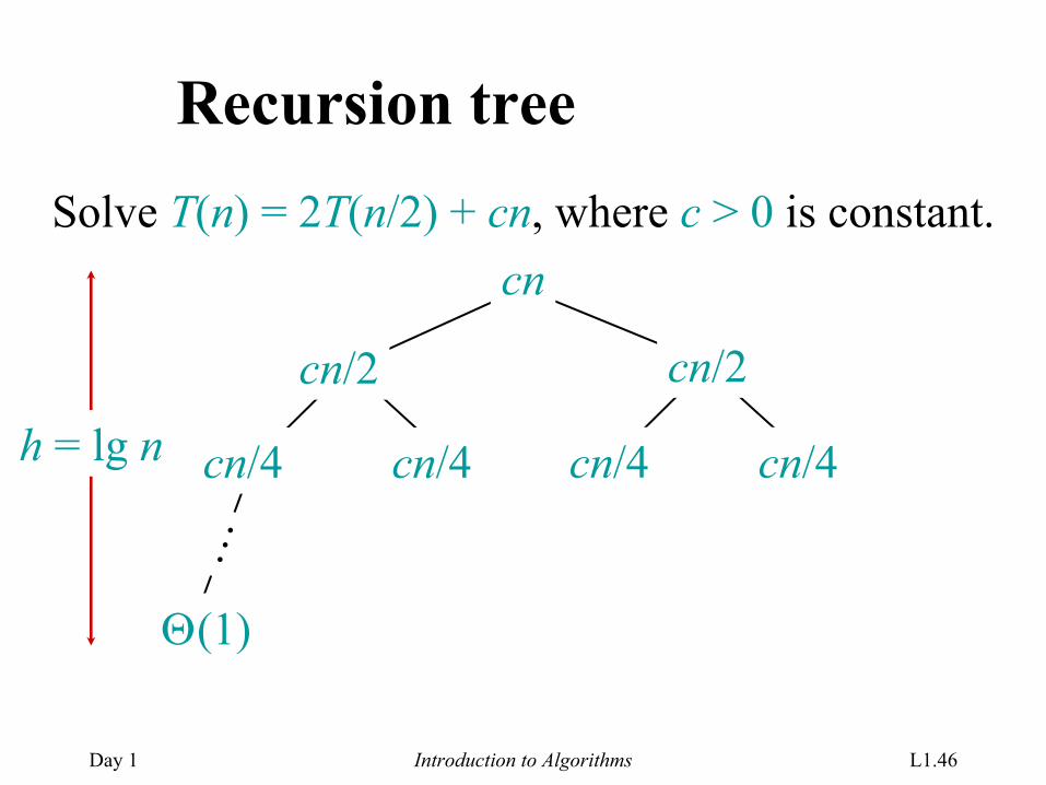
Day 1 Introduction to Algorithms L1.46
Recursion treeSolve T(n) = 2T(n/2) + cn, where c > 0 is constant.
cn
cn/4 cn/4 cn/4 cn/4
cn/2 cn/2
Θ(1)
…
h = lg n
Day 1 Introduction to Algorithms L1.47
Recursion treeSolve T(n) = 2T(n/2) + cn, where c > 0 is constant.
cn
cn/4 cn/4 cn/4 cn/4
cn/2 cn/2
Θ(1)
…
h = lg n
cn
Day 1 Introduction to Algorithms L1.48
Recursion treeSolve T(n) = 2T(n/2) + cn, where c > 0 is constant.
cn
cn/4 cn/4 cn/4 cn/4
cn/2 cn/2
Θ(1)
…
h = lg n
cn
cn
Day 1 Introduction to Algorithms L1.49
Recursion treeSolve T(n) = 2T(n/2) + cn, where c > 0 is constant.
cn
cn/4 cn/4 cn/4 cn/4
cn/2 cn/2
Θ(1)
…
h = lg n
cn
cn
cn
…
Day 1 Introduction to Algorithms L1.50
Recursion treeSolve T(n) = 2T(n/2) + cn, where c > 0 is constant.
cn
cn/4 cn/4 cn/4 cn/4
cn/2 cn/2
Θ(1)
…
h = lg n
cn
cn
cn
#leaves = n Θ(n)
…
Day 1 Introduction to Algorithms L1.51
Recursion treeSolve T(n) = 2T(n/2) + cn, where c > 0 is constant.
cn
cn/4 cn/4 cn/4 cn/4
cn/2 cn/2
Θ(1)
…
h = lg n
cn
cn
cn
#leaves = n Θ(n)Total = Θ(n lg n)
…
Day 1 Introduction to Algorithms L1.52
Conclusions
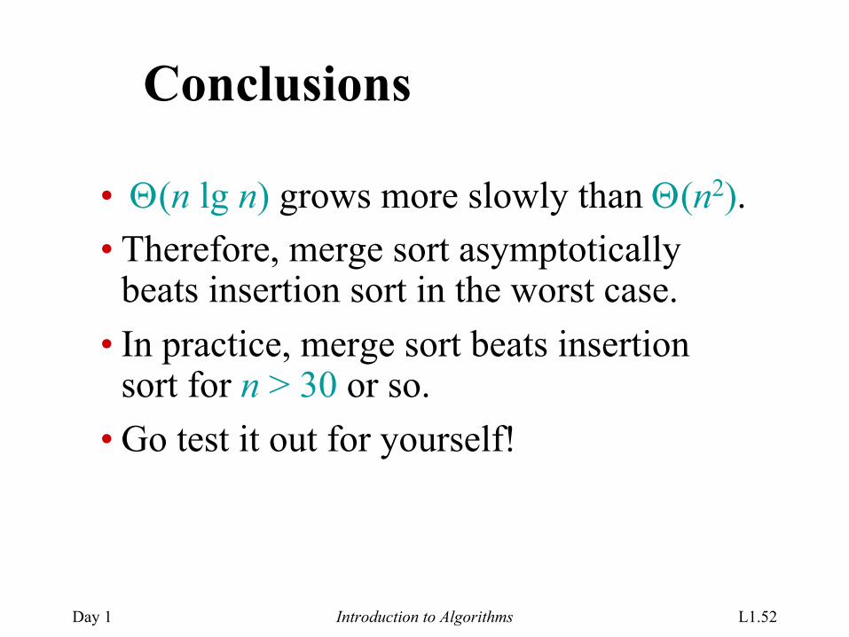
• Θ(n lg n) grows more slowly than Θ(n2).• Therefore, merge sort asymptotically
beats insertion sort in the worst case.• In practice, merge sort beats insertion
sort for n > 30 or so.• Go test it out for yourself!
Recommended