Intraday Liquidity Dynamics and Price Movements
Paolo Mazzaa
January 27, 2012
Working Paper
Abstract1
This study aims at analyzing whether intraday price movements help better characterize
liquidity in real time. We generate 15-minute price movement configurations based on2
Japanese candlesticks and measure liquidity in terms of spread, depth, order imbalance,3
dispersion and slope. We also consider trading activity and volatility measures. We find4
that Dojis and some Hammer-like configurations are associated with higher liquidity in5
the limit order book. The effects are short-lived but could enable traders to benefit from6
temporary higher liquidity. These results are robust to changes in the interval lengths.7
Our results suggest that the execution of trades could be improved when these particular8
structures appear on a price chart.9
JEL Classification: G1410
Keywords: Liquidity, Microstructure, Price Dynamics, Japanese Candlesticks11
a Paolo Mazza, Louvain School of Management & Catholic University of Louvain - UCL Mons, e-mail:
[email protected], 151 Chaussee de Binche - 7000 Mons (Belgium). We are grateful to NYSE12
Euronext in Paris for providing the data. We also thank Catherine D’Hondt, Rudy DeWinne, Jean-Yves Filbien,13
Christophe Majois, Mikael Petitjean and Gunther Wuyts for providing useful comments and suggestions. Any14
remaining errors are the responsibility of the author. The author gratefully acknowledges the support from the15
ARC grant 09/14-025.16

1 Introduction1
Liquidity has become of paramount importance in finance. The recent emergence of liquidity2
dark pools, algorithmic trading and, more generally, high frequency trading has drawn the3
attention of an increasing number of researchers and practitioners. The flash crash of May4
6th, 2010 is the best example of the implications of algorithmic trading, on the one hand,5
and the absence of liquidity, on the other hand. In such a trading environment and given6
the multidimensionality of liquidity, finding and estimating intraday liquidity in a fast and7
accurate way is a tough challenge.8
One solution to overcome this hurdle has been proposed by Kavajecz and Odders-White
(2004) who reveal some unexpected features of technical analysis. These authors examine9
similarities between support and resistance levels and the daily prices for which they observed10
high depth in the limit order book. They also study moving average indicators and check their11
information content in the order book. Based on NYSE stocks, their results show that signals12
in price charts are significantly related to the state of liquidity in the order book. They find13
that support and resistance levels and moving averages are strongly correlated with liquidity14
measured with customized indicators. The authors also conduct Granger causality tests, which15
reveal that technical analysis helps discover depth already present in the book.16
In this paper, we extend their analysis to High-Low-Open-Close price dynamics that prac-
titioners typically represent by drawing Japanese candlesticks. This method is an Eastern17
charting technique that is in essence very similar to bar charts. When looking at candlestick18
charts, traders have a quick snapshot of buying and selling pressures, as well as turning points.19
Using market data on a sample of European stocks of three national indexes, we study the re-20
lationship between liquidity and price movements by applying an event study methodology on21
15-minute time intervals for the best-known candlesticks structures. As outlined by Kavajecz22
and Odders-White (2004), price dynamics are expected to be linked with modifications in the23
state of the limit order book and with the supply of liquidity. For this purpose, we analyze24
different liquidity proxies: the relative spread, one-sided displayed and hidden depth measures25
(at the best bid and offer, at the five best limits, and for the whole book), order imbalances,26
dispersion measures, and the slope of the book. We also analyze the following trading activity27
measures: number and size of buyer and seller-initiated trades, as well as trade imbalances for28
number of trades and volumes. We first focus our analysis on the Doji structures which are29
the most influential single lines of the literature on Japanese candlesticks. The Dojis are also30
1

expected to have a direct impact on liquidity given the succession of price pressures that drive1
these signals. We then extent our analysis to other types of configurations.2
When a Doji appears on screen, our results suggest that liquidity is higher for all proxies
although there is less trading activity at that particular moment. The duration of the liquidity3
changes depends on the proxy but the patterns are always short-lived. This reinforces the4
hypothesis of an agreement on a price for the security, as exposed in the literature on Japanese5
candlesticks. This consensus implies a narrower spread, higher depth and less dispersion due6
to higher competition that liquidity suppliers face. The position of opening and closing prices7
on the candle is also related to different changes on bid and ask sides: bodies near the highest8
price of the interval are linked to changes at the ask while bodies near the lowest are related9
to changes at the bid. Using these dynamics might improve the execution of buy and sell10
decisions. Liquidity seems also to be higher when a Hammer or a Hanging Man occurs. In this11
respect, Japanese candlesticks may be used to have a quick idea on the state of liquidity in the12
limit order book. In a typical asset management firm, the decision to trade comes from the13
portfolio management team which then ask a broker to get the order executed in the best way.14
Japanese candlesticks may be used to have a quick idea on the state of liquidity in the limit15
order book. Trade execution could be improved by looking at these candlestick structures at16
the trade execution time. The magnitude of the potential gains on transaction costs is beyond17
the scope of this analysis and is left for further research.18
The remainder of the paper is organized as follows. Section 2 provides a brief review of the
literature on price dynamics, technical analysis and liquidity. Section 3 describes the dataset19
and the different liquidity measures that are used. Section 4 presents the methodology that we20
apply. Section 5 reports the findings of the event study and section 6 contains the robustness21
checks that are performed. The final section concludes.22
2 Literature review23
2.1 Liquidity and price dynamics24
Liquidity and order book dynamics have been at the core of several researches during the last25
decade. It is nevertheless still difficult to find a unique definition of liquidity in the literature.26
Demsetz (1968) first outlines the immediacy characteristic of liquidity, i.e. the immediate27
conversion of an asset into cash at the best available price. Campbell et al. (1997) define28
2

liquidity as ”the ability to buy or sell significant quantities of a security quickly, anonymously,1
and with relatively little price impact”. They also attribute four dimensions to liquidity:2
trading time (time between trades), depth (volume), tightness (spread) and resiliency (recovery3
from a liquidity shock).4
Blume et al. (1989) study the interactions between liquidity and price dynamics by in-5
vestigating the impact of order imbalances on stock price movements during the stock market6
crisis of October 19 and 20, 1987. The authors identify strong and positive correlation between7
order imbalances and price movements. The paper also enlightens a cascade effect of order8
imbalance on stock prices. The authors conclude that their results are consistent with the9
hypothesis that the stock decline was due to the incapacity of the market structure to absorb10
large selling orders. Using data from the Paris Bourse, Biais et al. (1995) investigate the supply11
and demand of liquidity as well as traders’ aggressiveness. They find that traders place orders12
inside the quotes when the spread or the depth (at the best quotes) is large. Chordia et al.13
(2001) empirically find that liquidity and trading activity are influenced by market returns and14
volatility. They also find that effective and quoted spreads increase dramatically in down mar-15
kets. This effect is asymmetric because spreads do not decrease much in up markets. Chordia16
et al. (2002) reach the same results and identify a significant impact of daily order imbalance17
on both market returns and volatility. They also state that it is unwise to trade when the order18
book is highly imbalanced if waiting costs are low. Chordia and Subrahmanyam (2004) present19
a theoretical framework for Chordia et al. (2001) and obtain the same results at the individual20
stock level. Harris and Panchapagesan (2005) also outline a relationship between the limit21
order book and future price movements using the TORQ database. Chan (2005) find evidence22
that order placement strategies depend on previous returns, i.e. traders are more aggressive23
in buying and place fewer sell orders after positive returns and conversely, a decrease in price24
cause sellers to be more aggressive by placing more orders at the best quotes, larger orders,25
or by reducing the spread. More recently, Chordia et al. (2008) find that short-term return26
predictability is lower when liquidity (as measured by the bid-ask spread) is higher. They also27
pointed out that prices have been more efficient after the change to decimal tick size, support-28
ing the positive relationship between liquidity and market efficiency. Cao et al. (2009) analyze29
the predictive power of limit order book information for 100 stocks quoted on the Australian30
Stock Exchange. They find evidence that it facilitates price discovery and is associated with31
future short-term returns. Boudt et al. (2012) also consider the dynamics of liquidity around32
price jumps and the information content of window formation in intraday price charts with an33
3
event study. They find that liquidity drops sharply and is particularly low at the time and in1
the following thirty minutes of a price jump.2
2.2 Market efficiency, price dynamics and Japanese candlesticks3
Papers on price dynamics abound in the literature. They are mainly related to the efficient-4
market hypothesis (EMH) developed in Fama (1970). There exists no consensus on efficiency:5
some argue that markets are sufficiently efficient while others find that there are punctual6
inefficiencies that allow traders to generate abnormal returns using information contained in7
past prices. Grossman and Stiglitz (1980) also argue that markets can be efficient if both8
informed and uninformed traders exist and if information is costly. So, the lack of consensus9
between proponents and opponents of efficiency contributes to market efficiency.10
The debates on the efficiency of financial markets have led to empirical research on stock
return predictability. One of the fields investigated is the so-called technical analysis, i.e.11
the study of past prices and their potential predictive power of future prices and returns.12
This concept is in contradiction with the weak-form efficiency of Fama (1970). Even here,13
the studies provide conflicting results. For instance, Brock et al. (1992) (henceforth BLL)14
find that moving averages and trading-range breaks generate statistically significant abnormal15
returns compared to four benchmark models, using a bootstrap methodology with the Dow16
Jones Industrial Average index. Bessembinder and Chan (1995), who test the profitability of17
technical analysis in Asian markets, also find evidence that their rules lead to abnormal returns18
and make the distinction between emerging and developed Asian markets, pointing out that19
returns are higher in emerging markets than in developed countries. Nevertheless, higher20
returns do not compensate for higher transaction costs incurred in both studies. Bessembinder21
and Chan (1998) also confirm the results of BLL but argue that market efficiency cannot be22
rejected due to return measurement errors arising from nonsynchronous trading, among other23
things. Sullivan et al. (1999) go beyond the analysis of BLL by testing 7846 trading rules with24
White’s Reality Check bootstrap methodology1 which offers a better control for data-snooping25
biases. The authors find that some of their trading rules perform even better than those of26
BLL. These studies are the best examples of stock return predictability research on technical27
analysis.28
During the last decade, the attention of some researchers has been drawn to Japanese
1White (2000).
4

candlesticks, another technical analysis charting method.2 Japanese candlesticks are a technical1
analysis charting technique based on High-Low-Open-Close prices. In that sense, they are2
similar to bar charts but they are easier to interpret. Indeed, the body is black for negative days3
(yin day) and white for positive days (yang day). Bar charts do not contain this information.4
The formation process of candlesticks appears in figure 1. There exist plenty of structures,5
formed by one to five candles, depending on the length of the shadows and the size and color6
of the bodies. These candlesticks emphasize what happened in the market at that particular7
moment. Each configuration can be translated into traders’ behaviors through price dynamics8
implied by buying and selling pressures.9
Figure 1: Candlestick formation process
Japanese candlesticks are interesting because they summarize a lot of information in one
single chart: the closing price, the opening price as well as the lowest and highest prices.10
With the raising interest in high frequency trading and the narrowing of trading intervals,11
they have been increasingly used by practitioners to capture short term price dynamics. As12
for technical analysis, papers addressing candlesticks enter in the ”stock return predictability”13
2Even if they have been used for centuries in eastern countries, Steve Nison was the first to bring this methodto the west in the nineties. Japanese candlesticks have been first used by Munehisa Homma who traded in therice market during the seventieth century. The original names of the candlestick structures come from the waratmosphere reigning in Japan at that time. At the beginning, there were only basic structures from one tothree candles but more complex configurations have been identified since then. The predictive power of theseconfigurations is still discussed. Nison (1991), Nison (1994), Morris (1995) and Bigalow (2001) are the bestknown and used handbooks of candlestick charting.
5

category. Marshall et al. (2006) and Marshall et al. (2008) find no evidence that candlesticks1
have predictive value for the Dow Jones Industrial Average stocks and for the Japanese equity2
market, respectively. They replicate daily data with a bootstrap methodology similar to the3
one used in Brock et al. (1992). However, intraday data is more relevant as traders do not4
typically wait for the closing of the day to place an order. Using intraday candlesticks charts on5
two future contracts (the DAX stock index contract and the Bund interest rate future), Fock6
et al. (2005) still find no evidence which suggests that candlesticks, alone or in combination7
with other methods, have a predictive ability. However, none of these papers looks at the8
relationships between candlestick configurations and order book dynamics.9
Previous research has outlined strong relationships between price movements and trade
measures (e.g. Blume et al. (1989)). As candlesticks are good proxies for representing High-10
Low-Open-Close prices dynamics, we also expect a relationship between the occurrence of11
particular structures and trading activity measures. Fiess and MacDonald (2002) also argue12
in favor of that point. A relation between candlestick configurations and liquidity measures is13
also expected as trading activity measures are linked to the state of the order book, i.e. a trade14
occurs when supply meets demand and this matching is realized through the limit order book.15
The occurrence of some particular single lines should also be related to direct modifications in16
the book. This is the case of the Doji structures.17
The Doji is one of the core structures of Japanese candlesticks. A Doji appears when the
closing price is (almost) equal to the opening price. Candlestick books3 refer to it as the magic18
Doji. We observe different types of Dojis.4 The most frequent Doji is a ”plus”, i.e. no real19
body and almost equal shadows. If both closing and opening prices are also the highest price20
of the interval, the Doji becomes a Dragonfly Doji. By contrast, it becomes a Gravestone Doji21
when both closing and opening prices are equal to the lowest price of the interval. Another22
characteristic of the Doji is the position. A Doji may appear in a star position which means23
that a gap exists between the Doji and the previous candle. These Dojis are mostly part of24
the abandoned babies structures. A Doji may also occur in a Harami position when it appears25
within the previous body.26
The Doji denotes moments where markets are on a rest and where there exists an agreement
on the price of the stock. In this situation, traders are likely to situate the price of the stock27
inside the spread, leading to competition among traders which reduces the spread and the28
3Nison (1991), Nison (1994) and Morris (1995).4A description of the presented structures is available in appendix.
6

dispersion while increasing the slope and best quotes quantities. As a consequence, we expect1
liquidity to be higher and trading activity to be lower. We expect our results to be short-lived2
and the dynamics to appear in the window [-1;+1]. We also expect different outcomes between3
Gravestone and Dragonfly Dojis as they come from different succession of price pressures: the4
Gravestone (Dragonfly) is made with a previous bullish (bearish) rally and ends up with a5
strong selling (buying) pressure.6
3 Data7
3.1 Data and Sample8
We use Euronext market data on 81 stocks belonging to three national indexes: BEL20, AEX9
or CAC40. We have tick-by-tick data for 61 trading days from February 1, 2006 to April 30,10
2006. This database enables us to compute different measures from the order book and from11
trades. We also dispose on undisclosed data on hidden orders.512
We have rebuilt High-Low-Open-Close prices from this database for the 81 stocks over
the whole sample period. As tick data are not adapted for candlesticks analysis, we built13
15-minute-intervals which leads to 34 intervals a day. This interval length is the best trade-14
off which allows to include intraday trends and to avoid noisy candlesticks patterns resulting15
from non-trading intervals. We use the HLOC prices calculated above in order to identify16
candlestick configurations with the help of the TA-Lib.6 We have a total of 167068 records (8117
firms, 61 days, 34 intervals/day) in our dataset.18
We filter the sample as follows. First, we remove Four Prices Dojis because they are
associated with non-trading patterns.7 Second, we only keep the events for which we do not19
5Hidden orders are orders that gradually display part of their total amount. For instance, a hidden orderof 500 may appear on the book with a quantity of 100 and will automatically be refilled when 100 shares havebeen consumed.
6The TA-lib library is compatible with the MATLAB Software and returns, for each type of configurationand for each record, ”1” if the bullish part of the structure is identified, ”-1” for the bearish part and ”0”otherwise. As the structures are bullish, bearish or both, for each event type, the values that may appearare [0 ; 1], [-1 ; 0] or [-1 ; 0 ; 1]. The TA-lib allows some flexibility in the recognition of the configurations.As it is an open source library, we have been able to check the parametrization of the structures. Events arerecognized according to the flexibility rules presented in Nison (1991) and Morris (1995). The TA-lib contains61 pre-programmed structures. We however dropped 17 of them due to a lack of intraday significance. The listof these configurations is available upon request.
7A Four Prices Doji occurs when all the prices are equal. When they occur in daily, weekly or monthly charts,they are a strong clue of a potential reversal. However, in intraday price charts, they represent non-tradingintervals.
7

observe any other structure in the previous and next three intervals in order to avoid any1
contagion effect in our measures. Therefore, there is only one event by analyzed window.8 As2
we study a moving window of [-3;+3], we do not consider events in the first and last three3
intervals for each day. Finally, we only keep events types for which we have at least 30 event4
occurrences.5
After the removal of all the possible contagious data, we have a total of 2959 Dojis, among
which 653 are Dragonfly Dojis and 614 are Gravestone Dojis. Table 1 shows event occurrences.6
Table 1: Events Count
Name Bull/Bear Count
Doji 1 2959Bearish Dojistar -1 111Bullish Dojistar 1 121Dragonfly Doji 1 653Gravestone Doji 1 614
We look at the occurrences of the identified structures and check whether some configura-
tions appear at a particular moment during the day. Figure 2 displays the intraday pattern7
of our events. The distribution seems to peak at both the first and last moments of the day.8
Figure 3 shows that these results come from many Dojis occurring at these particular moments.9
Figure 2: Events by Interval
This figure displays the number of events in each time interval.
8We keep the 44 configurations from the TA-lib for this filter.
8

Figure 3: Dojis by Interval
This figure displays the number of Dojis in each time interval.
3.2 Liquidity Measures1
We measure liquidity at the end of each trading interval which enables us to measure the direct2
impact of the event on liquidity. We first calculate the traditional liquidity proxies such as3
relative spread, depths (displayed and hidden, in number of shares) and order imbalances (at4
different order book levels). We also use dispersion and slope measures which are respectively5
presented in Kang and Yeo (2008) and Næs and Skjeltorp (2006). Then, we compute trading6
activity measures as buyer and seller-initiated volumes and imbalances, in number of trades7
and quantities.9 Finally, we evaluate volatility using the High-Low measure for each time8
interval.10 Table 2 presents the different measures.9
9These measures are computed with the sum over each interval.10We also study the squared return as a volatility measure but the results are very similar.
9

Tab
le2:
Liquidityproxiesandtradingactivitymeasures
Name
Med
ian
Name
Med
ian
Quantities
attheBestBid
1978.00
5BestLim
itsHidden
Imbalance
0.04
Quantities
attheBestAsk
1953.00
Imbalance
Total
0.11
Quantities
attheBestBid
(Hidden
)0.00
Imbalance
Displayed
0.16
Quantities
attheBestAsk
(Hidden
)0.00
Imbalance
Hidden
0.02
Displayed
Dep
th5BestBid
13409.00
Number
ofbuyer-initiatedtrades
28.00
Displayed
Dep
th5BestAsk
13612.00
Quantities
ofbuyer-initiatedtrades
12785.00
Hidden
Dep
th5BestBid
1559.00
Number
ofseller-initiatedtrades
31.00
Hidden
Dep
th5BestAsk
1800.00
Quantities
ofseller-initiatedtrades
13508.00
Displayed
Dep
thBid
312453.50
Imbalance
Number
ofTrades
-0.05
Displayed
Dep
thAsk
361465.00
Imbalance
Traded
Quantities
-0.03
Hidden
Dep
thBid
130558.50
High-Low
0.00
Hidden
Dep
thAsk
143938.00
SquaredReturn
0.00
TotalDep
thBid
169410.00
DispersionBid
0.02
TotalDep
thAsk
212337.00
DispersionAsk
0.02
Dep
thFirst
Lim
its(B
id+ask)
4541.50
Dispersion
0.02
Hidden
Dep
thFirst
Lim
its(B
id+ask)
453.00
Imbalance
Dispersion
0.00
Dep
th5First
Lim
its(B
id+ask)
27908.00
Bid
Slope
4245.62
Hidden
Dep
th5First
Lim
its(B
id+ask)
8410.50
Ask
Slope
4269.39
Totaldep
th(B
id+ask)
387121.50
Slope
4302.42
Hidden
Totaldep
th(B
id+ask)
280698.00
RelativeSpread
0.07
First
Lim
itsIm
balance
0.00
Buy-sideAggressiven
ess
-0.42
First
limitsHidden
Imbalance
-0.04
Sell-sideAggressiven
ess
-0.37
5BestLim
itsIm
balance
0.01
Quantities
atth
ebestbid
(ask)den
otesth
eamountofsh
aresdisplayed
atth
ebestbid
(ask)limit.Hidden
indicatesth
equantities
thatare
notdisplayed
.Displayed
Dep
th5BestBid
(Ask)represents
thetotalamountdisplayed
atth
efivebestbid
(ask)limits.
Hidden
Dep
th5BestBid
den
otesth
etotalhidden
amountatth
efivebestbid
(ask)limits.
Displayed
Dep
thBid
(ask)standsforth
etotalamountofsh
aresth
atis
displayed
onth
ebid
(ask)sideofth
eord
erbook.Hidden
Dep
thBid
(ask)only
includes
hidden
quantities
atth
ebid
(ask)whileTotalDep
thBid
(ask)is
thesu
mofboth
displayed
andhidden
totaldep
thsatth
ebid
(ask).
Dep
thFirst
Lim
its(B
id+ask)is
thesu
mofdisplayed
bestbid
andoffer
quantities.Hidden
Dep
thFirst
Lim
its(B
id+ask)only
takes
into
accounthidden
quantities.Dep
th5First
Lim
its(B
id+ask)andHidden
Dep
th5First
Lim
its(B
id+ask)are
computedacross
thefivebestprice
limitswhileTotaldep
th(B
id+ask)andHidden
Total
dep
th(B
id+ask)co
nsider
thewhole
book.First
limitsIm
balance
isth
ebestlimitsdisplayed
imbalance
(Imba
lance
i,t=
Depth
Bid
i,t−D
epth
Aski,t
Depth
Bid
i,t+D
epth
Aski,t,whereiden
otesa
given
secu
rity
andtagiven
interval.).
First
limitsHidden
Imbalance
only
considershidden
quantities.Thesamemea
suresare
computedforth
efivebestlimits(5
BestLim
itsIm
balance
and5BestLim
itsHidden
Imbalance)aswellasforth
ewhole
book(Imbalance
Displayed
andIm
balance
Hidden
).Im
balance
Totalis
thetotal
imbalance,su
mmingdisplayed
andhidden
quantities.
10
Dispersion Kang and Yeo (2008) present two measures to quantify the density of the limit1
order book, i.e. how limits are far from each other or from the quoted midpoint. One of these2
two measures is the dispersion:3
Dispersioni,t =1
2
(∑nj=1w
Bidi,j,tDstBid
i,j,t∑nj=1w
Bidi,j,t
+
∑nj=1w
Aski,j,tDstAsk
i,j,t∑nj=1w
Aski,j,t
), (3.1)
where, for security i and interval t, wi,j,t are the weights which are equal to quantities,
offer and bid sizes, at the jth price limit normalized by the total depth of the five best limits,4
DstBidi,j,t = (PBi,j−1,t − PBi,j,t) and, DstAsk
i,j,t = (PAi,j,t − PAi,j−1,t). The midquote is used for5
the distance of the first best limits.6
As Kang and Yeo (2008) outline, dispersion is small under fierce competition as each trader
wants to gain price priority.7
Slope The slope is computed by averaging the price elasticity of quantities over the five best8
quotes. We calculate the slope of the book following Næs and Skjeltorp (2006), that is:9
SLOPEi,t =DEi,t + SEi,t
2, (3.2)
where DEi,t and SEi,t are the slope of the bid and ask side respectively and are computed as:10
DEi,t =1
5
(vB1
|pB1 /p0 − 1|+
NB∑τ=1
vBτ+1/vBτ − 1
|pBτ+1/pBτ − 1|
), (3.3)
SEi,t =1
5
(vA1
pA1 /p0 − 1+
NA∑τ=1
vAτ+1/vAτ − 1
pAτ+1/pAτ − 1
). (3.4)
pBτ and pAτ are the prices, respectively at the bid and at the ask, appearing at the quote τ .11
p0 denotes the quoted midpoint. Finally, vBτ and vAτ are the natural logarithm of accumulated12
total share volume at the limit τ respectively for the bid and the ask11.13
A steep slope represents an order book where volumes are concentrated at a given limit
(low elasticity) while a gentle slope denotes an order book where volumes are not aggregated14
11By accumulated, we mean the sum of the quantities outstanding at that limit and the sum of all quantitiesoutstanding at each better quote.
11

at a given limit (high elasticity). A steep slope also means that traders agree about the value1
of the security while a more gentle slope indicates that traders have different estimations of2
the fair price of the security.3
Trade Imbalance In order to calculate trade imbalance, we first have to sign transactions.4
Most empirical studies use Lee and Ready (1991)’s algorithm, which categorizes buyer and5
seller-initiated trades based on the position of the transaction price relative to the bid-ask6
spread. With our database, we are able to match for each transaction the orders that generate7
a given trade. Then, the sign of the transaction is found by comparing the submission time8
of the orders, i.e. the last order being the determinant of the transaction. After that, we9
compute the total number of trades and quantities respectively for buyer and seller-initiated10
trades. With these variables, we compute two trade imbalance measures:11
ImbalanceNi,t =NTradesBuy
i,t −NTradesSelli,t
NTradesBuyi,t +NTradesSelli,t
(3.5)
where NTradesBuyi,t is the number of buyer-initiated trades occurring at the tth interval for12
stock i and NTradesSelli,t is the number of seller-initiated trades occurring at the tth interval13
for stock i.14
ImbalanceQi,t =QBuy
i,t −QSelli,t
QBuyi,t +QSell
i,t
(3.6)
where QBuyi,t is the sum of the volume of all buyer-initiated trades occurring at the tth interval15
for stock i and QSelli,t is the sum of the volume of all seller-initiated trades occurring at the tth16
interval for stock i.17
These measures are computed separately for each interval and for each security. As we also
dispose on the buyer and seller-initiated quantities and number of trades, we also include them18
in the analysis.19
Aggressiveness We compute our aggressiveness measure separately for bid and ask sides.20
Our measure captures the number of aggressive orders, i.e. orders that consume liquidity and21
generate a trade, compared to the total of orders that occurs during a given time interval:22
12

AggressivenessBi,t =NbAggressiveBuy
i,t −NbPassiveBuyi,t
NbAggressiveBuyi,t +NbPassiveBuy
i,t
(3.7)
where NbAggressiveBuyi,t is the total number of marketable buy orders occurring at the tth1
interval for stock i and NbPassiveBuyi,t is the total number of non-marketable buy orders2
occurring at the tth interval for stock i. A similar process is applied to sell orders.3
4 Methodology4
With our extended dataset containing HLOC prices, candlestick identification variables and5
liquidity measures, we conduct an event study of liquidity behavior around candlestick struc-6
tures. We focus on a time window of [-3,+3] containing seven observations: three observations7
before the signal, the time of the signal and three observations after the signal. This leads us8
to consider liquidity behavior 45 minutes before and after our events. As we have different9
types of measures, we compute our abnormal liquidity measures depending upon the nature10
of the variables, as suggested by Boudt et al. (2012).11
For spreads, imbalances and aggressiveness measures, we compute the abnormal measure
as follows:12
Abnormali,t,m = Measurei,t,m −MedianNEi,t,m, (4.1)
where Measurei,t,m is the analyzed liquidity measure m for stock i for the time interval t and
MedianNEi,t,m is the median of the measure m for stock i across all non-events12 occurring during13
the time interval t.14
For the other measures, the calculation method is:15
Abnormali,t,m =Measurei,t,m −MedianNE
i,t,m
MedianNEi,t,m
, (4.2)
where Measurei,t,m is the analyzed liquidity measure for stock i for the time interval t and
MedianNEi,t,m is the median of the measure m for stock i across all non-events occurring during16
the time interval t.17
12The 17 dropped pre-programmed structures have been included in the non-event sample as they are toofrequent on intraday data and are not linked to any particular signal.
13

We apply these processes separately for each liquidity measure. We then aggregate the
results obtained on a stock basis to form median patterns of liquidity behavior around each1
event and for each measure. We analyze these patterns to check whether the abnormal measures2
are significantly different from zero. For this purpose, we use a standard non parametric3
sign test on the controlled measures. Our null hypothesis postulates that the median of the4
abnormal measure equals zero. The statistic M is computed as follows:5
M =N+ −N−
2, (4.3)
where M follows a binomial distribution, N+ is the number of positive values and N− is the
number of negative values. Values equal to zero are discarded.6
We then analyze the p-values of each time interval of the window and check whether
the differences are significant or not. If the p-value at the signal interval is significant, the7
structure is associated to a particular state of (il)liquidity. This signal may thus lead to a8
given configuration of the limit order book. If p-values are significant before the signal, the9
signal may be a response to a particular state of liquidity. If p-values are significant after the10
signal, a change of liquidity may correspond to a response to the signal.11
5 Results12
5.1 Doji13
5.1.1 Overall picture14
In a nutshell, the results show that liquidity is higher when a Doji appears, confirming our15
hypotheses. A higher liquidity and fewer trades mean that a consensus exists on the price of16
the stock and that buyers and sellers are not willing to trade at a different price. They do17
not want to hit the best opposite quote. A Doji is an indication of the presence of liquidity18
on each side of the book. Placing liquidity-taking orders at that moment will thus cost less19
in terms of implicit costs. Liquidity providers are also numerous and, as a consequence, face20
more competition to supply liquidity.21
However, these results are valid only without the presence of jumps. Boudt et al. (2012)
argue that jumps are linked to illiquid states of the book. We may thus consider that candles in22
14

Harami position are linked to liquidity while star positions, i.e. jumps, are linked to illiquidity.1
We tested this hypothesis by comparing Harami Dojis and Doji Stars.13 We confirm that the2
Doji in star position are linked to less liquid states of the book than for Harami Dojis.143
Furthermore, identifying the type of Doji also brings interesting information about the
heaviness of one side of the book. The Dragonfly Doji seems to be associated to more changes4
at the ask and the Gravestone Doji seems to be linked to changes at the bid. These movements5
occur about 15 minutes before the occurrence of these Dojis, implying that the Doji itself is6
the consequence of depth dynamics. This result is confirmed by imbalances which show that7
the order book is imbalanced before these Dojis and returns to more normal values after the8
occurrence of the Dojis. We also observe disparities regarding trades. While buyer-initiated9
trades are less frequent and smaller in size when there is a Gravestone Doji, seller-initiated10
trades are less frequent and smaller in size when a Dragonfly Doji occurs. Buy orders are also11
more aggressive after a Dragonfly Doji and sell orders are more aggressive when a Gravestone12
Doji appears.13
Our analysis finally shows that liquidity is negatively correlated with volatility as the High-
Low is significantly lower while liquidity seems to be higher when a Doji appears. This result14
contributes to the literature on the liquidity-volatility relationship.15
13We disentangle Bullish and Bearish parts of the configurations as they may have a totally different impact.14The drop in liquidity is effective in terms of spread, depth, dispersion and slope. These results are not
reported here but are available upon request.
15

5.1.2 Details1
Figure 4: Abnormal spread around Doji
Full, doted and dashed lines represent the intra-window median pattern for the abnormal spread respectively for the Doji,
the Dragonfly Doji and the Gravestone Doji. Triangles (△), squares (�), and circles (◦) indicate a rejection of the null
hypothesis respectively at the 99%, 95% and 90% confidence levels.
The spread significantly drops when a Doji appears. The recovery is fast after the trough in all cases. This is perfectly
in line with what we expected as a Doji occurs when there is a consensus on the price. Traders seem to agree on a price
for the stock and situate it inside the spread. A reduction of the spread confirms this consensus.
16

Figure 5: Abnormal depth around Doji
(a) Best bid (b) Best Ask
(c) First quote (Both sides) (d) Five quotes (Both sides)
Full, doted and dashed lines represent the intra-window median pattern for each of the abnormal depth measures mentioned
respectively for the Doji, the Dragonfly Doji and the Gravestone Doji. Triangles (△), squares (�), and circles (◦) indicatea rejection of the null hypothesis respectively at the 99%, 95% and 90% confidence levels.
The quantities at the best bid are significantly higher, at a 1% confidence level, at the time of the signal. Quantities
at the best bid are also significantly higher just before the apparition of a Gravestone Doji. The pattern at the ask is
more noisy but indicates that the Dragonfly Doji presents a significantly higher best ask depth just before its occurrence.
These Dojis seem to be the consequences of a particular state of liquidity in the limit order book as the pattern starts
in t-1. The Gravestone Doji is likely to occur just after an accumulation of depth at the bid that does not translate into
more trades. The Dragonfly Doji seems to appear when depth at the ask is higher and when there are less trades. The
results of the bid side are confirmed if we consider the five best quotes. However it is not the case for the ask side. If we
look at the sum of both sides, we also observe a peaking depth for the first quote and for the five best quotes. This is
interesting as the reduction of the spread does not take place at the cost of a lower depth. Liquidity is higher over these
two dimensions.
17

Figure 6: Abnormal Hidden Depth (Sum)
(a) Five best bid limits (b) Five best ask limits
Full, doted and dashed lines represent the intra-window median pattern for each of the abnormal hidden depth measures
mentioned respectively for the Doji, the Dragonfly Doji and the Gravestone Doji. Triangles (△), squares (�), and circles
(◦) indicate a rejection of the null hypothesis respectively at the 99%, 95% and 90% confidence levels.
The Gravestone Doji presents a peak in hidden depth at the bid just before its apparition while depth at the ask peaks
just before the Dragonfly Doji. These findings indicate that the position of the real body (near the highest or lowest price
of the time interval) on the candle has a one-sided impact on depth, hidden or not.
18

Figure 7: Abnormal imbalance around Doji
(a) Displayed best bid and offer (b) Hidden best bid and offer
(c) Displayed five best limits (d) Hidden five best limits
Full, doted and dashed lines represent the intra-window median pattern for each of the abnormal imbalances respectively
for the Doji, the Dragonfly Doji and the Gravestone Doji. Triangles (△), squares (�), and circles (◦) indicate a rejection
of the null hypothesis respectively at the 99%, 95% and 90% confidence levels.
We observe opposite patterns for the Dragonfly and Gravestone Dojis. Order book imbalance is significantly higher just
before and when a Gravestone Doji appears while it is significantly lower before and when a Dragonfly Doji occurs. The
simple Doji does not exhibit any particular pattern.
19

Figure 8: Abnormal dispersion around Doji
(a) Dispersion : Bid side (b) Dispersion : Ask side
(c) Dispersion
Full, doted and dashed lines represent the intra-window median pattern for each of the abnormal dispersion respectively
for the Doji, the Dragonfly Doji and the Gravestone Doji. Triangles (△), squares (�), and circles (◦) indicate a rejection
of the null hypothesis respectively at the 99%, 95% and 90% confidence levels.
The dispersion drops when a Doji appears, meaning that the competition in the book is higher at that particular moment
and that the limits are closer from each other. This is consistent with the idea of consensus. Traders are also competing
to gain price priority implying a narrower spread. If we disentangle ask and bid sides, we observe that dispersion is
significantly lower at the bid for the Dragonfly Doji and at the ask for the Gravestone Doji while it remains unchanged
on the other side. These findings are also coherent with the philosophy behind these two Dojis: a strong buying pressure
creates the Dragonfly Doji while the Gravestone Doji appears after a selling rally. This is also in line with the one-sided
impact that occurs for depth.
20

Figure 9: Abnormal slope around Doji
(a) Supply (b) Demand
(c) Slope
Full, doted and dashed lines represent the intra-window median pattern for each of the abnormal slope respectively for
the Doji, the Dragonfly Doji and the Gravestone Doji. Triangles (△), squares (�), and circles (◦) indicate a rejection of
the null hypothesis respectively at the 99%, 95% and 90% confidence levels.
The slope significantly peaks at the moment of the Doji, on both supply and demand sides. These outcomes are consistent
with the agreement on the price and with dispersion measures which show an increase in order book density when these
signals appear.
21

Figure 10: Abnormal Number of trades around Doji
(a) Number of buy trades (b) Number of sell trades
(c) Imbalance
Full, doted and dashed lines represent the intra-window median pattern for this trading activity measure respectively for
the Doji, the Dragonfly Doji and the Gravestone Doji. Triangles (△), squares (�), and circles (◦) indicate a rejection of
the null hypothesis respectively at the 99%, 95% and 90% confidence levels.
The number of trades is lower when the signal appears, whatever the direction of the trade. After the signal, there is a
quicker return to normal values for buy trades than for sell trades which remain low 15 minutes after the signal. Traders
seem to delay buying and selling activities when these signals occur, even if liquidity is higher. As depth does not fall
and even increase, there are more pending orders in the book. If we investigate the pattern for the Gravestone and the
Dragonfly Doji and keeping in mind the philosophy behind these structures, we observe that buy trades are less numerous
and less big for the Gravestone Doji compared to sell trades while we observe the opposite pattern for the Dragonfly Doji.
Since, the Gravestone Doji appears when a selling rally follows a strong buying pressure, our results suggest that the
selling rally does not come from an increased sell volume but from a decrease in buy volume. The opposite interpretation
may be done for the Dragonfly Doji. Trade imbalances confirm these findings with a sharp drop for the Gravestone Doji
and a significant peak for the Dragonfly Doji.
22

Figure 11: Abnormal aggressiveness around Doji
(a) Buyers (b) Sellers
Full, doted and dashed lines represent the intra-window median pattern for these aggressiveness measures respectively for
the Doji, the Dragonfly Doji and the Gravestone Doji. Triangles (△), squares (�), and circles (◦) indicate a rejection of
the null hypothesis respectively at the 99%, 95% and 90% confidence levels.
Sell orders are more aggressive when a Doji appears while buy orders are more aggressive only 15 minutes after the
apparition of the Doji. Traders seem to place more marketable orders than they usually do, even if trading activity
is lower. This suggest that buy traders become aggressive after the apparition of the Doji. Sellers react quicker than
buyers do. The results also suggest that sellers are even more aggressive when the Doji is a Gravestone Doji and buyers
seem to be even more aggressive in the case of a Dragonfly Doji. These results are at first sight not consistent with the
lower trading activity around these structures. Yet, even if traders are less numerous, they are more aggressive but their
aggressiveness does not erode depth at the opposite side.
23

Figure 12: Abnormal High-Low around Doji
Full, doted and dashed lines represent the intra-window median pattern for the volatility measured with the high-low
range respectively for the Doji, the Dragonfly Doji and the Gravestone Doji. Triangles (△), squares (�), and circles (◦)indicate a rejection of the null hypothesis respectively at the 99%, 95% and 90% confidence levels.
Whatever the Doji structure, the High-Low volatility measure sharply falls when the signal appears. The level is significant
at 1%. A Doji is thus linked to lower volatility, which is consistent with the consensus on the price implied by the Doji.
This also indicates that high volatility Dojis, Doji with very long shadows, are very rare in our dataset.
6 Robustness checks1
In this section, we first investigate other types of dynamics by looking at Hammer-like con-2
figurations. Among Hammer-like structures, there are four structures that are characterized3
by a long shadow and a small real body.15 The Hammer appears at the end of a downtrend4
and is made of a very small real body with (almost) no upper shadow and a very long lower5
shadow. The same structure may appear at the end of an uptrend but, in that case, it is called6
a Hanging Man. Inverting the shadows, i.e. the upper shadow becomes the lower shadow and7
vice-versa, we obtain an Inverted Hammer at the end of a downtrend or a Shooting Star at the8
end of an uptrend. This group of figures is interesting for many purposes. First, as these figures9
are said to be strong reversal structures, we expect a high correlation between changes in trade10
imbalances and the occurrence of these structures. Regarding liquidity, the results should be11
linked to previous findings on the Gravestone and Dragonfly Dojis if the size of the real body12
has little impact. Indeed, a Dragonfly Doji may be a particular Hammer or Hanging Man13
while a Gravestone Doji may be a particular Inverted Hammer or Shooting Star, depending on14
their position on the price chart. If we observe differences between these structures, the size15
15A description of the presented structures is available in appendix.
24

of the real body has an influence on liquidity behavior. We also expect a difference between1
bullish and bearish signals. Hammers and Inverted Hammers should present some similarities2
in their results as well as Hanging Men and Shooting Stars.3
Then, we conduct the same analysis on candlesticks generated from 30-minutes and 60-
minutes price series. By doing this, we create two new sets of events. This enables us to check4
whether our findings are the consequence of the choice of the time interval.165
6.1 The Hammer, the Hanging Man, the Inverted Hammer and the Shoot-
ing Star6
In a nutshell, our results confirm the literature on Japanese candlesticks which states that7
Hammer-like configurations are strong reversal structures as they really break the intra-window8
pattern. We observe a higher liquidity just before the formation of the Hammer but this9
liquidity is not provided by more depth: the book is more dense and the spread is lower. The10
Hanging Man also shows similar outcomes but only after it has fully appeared on the chart.11
The results we discuss here may come from the configuration type, i.e. the size of the shadows.12
This is confirmed by the order imbalance results which show that the order imbalance is more13
in favor of the ask when the lower shadow is longer. Trading activity and aggressiveness14
measures are totally in line with the bearish or bullish reversal potential of the structure. We15
also observe lower volatility when these structures appear. The results are summarized in16
Table 3.17
16All the graphs of this analysis are not presented here but are available upon request.
25

Table
3:LiquiditydynamicsaroundHammer-likeconfigu
rations
Hammer
(625)
InvertedHammer
(175)
HangingMan(469)
ShootingStar(91)
-10
1-1
01
-10
1-1
01
Spread
–3
-2
+++
3-
2--
1-
2+++
2
Bid
dep
th-
3--
3-1
+++
3++
--
Ask
dep
th+++
3+++
3
Imbalance
---
3+++
2---
3
Dispersion-Bid
+++
1--
2---
3-
2+
1
Dispersion-Ask
---
3+++
3+++
3
Slope-Bid
+++
3---
3++
3+++
3--
2
Slope-Ask
+++
3---
3+++
3+++
3++
2--
2
This
table
presents
theresu
ltsobtained
forth
efourHammer-likestru
cturesforea
chliquiditymea
sure.
Each
panel
represents
a[-1;+
1]timewindow
around
the
occurren
ceofth
eev
ent.
”+”and”-”
signsden
ote
positiveandneg
ativevalues
forth
eabnorm
almea
sure.”++”and”–”signsden
ote
bigger
positiveandneg
ative
variations.
”+++”and”—
”signsden
ote
pea
ksandtroughover
thetimewindow.Theex
ponen
tsden
ote
thesignifica
nce:1for10%
significa
nce,2for5%
significa
nce
and3for1%
significa
nce.
Theresu
ltsclea
rlyindicate
thatliquidityis
higher
before
theapparition
ofth
eHammer
and
when
theHangingMan
occurs.Liquidityseem
salsoto
belower
for
theInvertedHammer
andth
eShootingStar.
Dep
thresu
ltssu
ggestth
atch
anges
inliquidityaroundth
esestru
cturesare
only
one-sided
.Theseoutcomes
are
similar
toth
ose
ofth
eDoji
stru
cturesforwhich
bid
and
ask
quantities
evolvedifferen
tlydep
endingon
theposition
ofth
eprice
on
theca
ndle
(nea
rth
ehighestorlowest
ofth
einterval).Theim
balance
significa
ntlydropsjust
before
aHammer
oraHangingMan.Thebookseem
sto
beim
balancedin
favorofth
eask
sidewhen
these
configurationsappea
r,co
nfirm
ingpreviousresu
lts.
Reg
ard
ingdispersion,weobserveth
atth
eHammer
presentash
arp
dropin
dispersionatth
eask
just
before
its
occurren
ce.This
maysu
ggestth
atth
elength
ofth
esh
adowshasalsoanim
pact
ondispersion.A
Hammer
islikelyto
occurwhen
theden
sity
ofth
eask
sideincrea
ses,
i.e.
price
limitsare
closerfrom
each
oth
er.This
isco
nsisten
twithanagreem
entonth
eminim
um
price
andth
een
dofth
ebea
rish
rally.
Asex
pected,th
esestru
ctures
exhibitch
anges
indispersiongiven
theirhighreversalpotential.
Sloperesu
ltsare
totaly
inlinewithdispersionresu
lts.
Number
ofbuyandselltrades,tradeim
balance,
agressiven
essandvolatility
mea
suresare
consisten
twithth
eliteratu
reonJapaneseca
ndlesticksandwithth
eprice
pressuresth
atdriveth
esesignals.Thereare
thus
notreported
here.
26
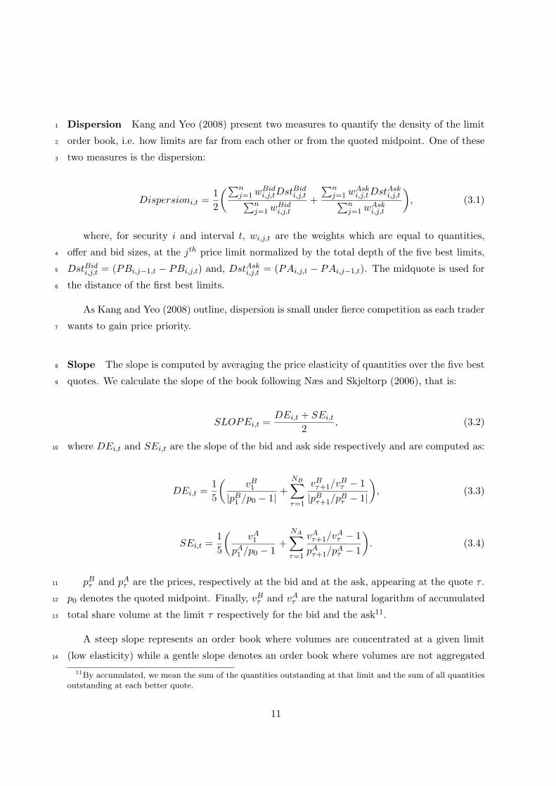
6.2 Changing the time interval1
Table 4 presents the number of occurrences for each structure for both 30-minutes and 60-2
minutes price series.3
Table 4: Events count for 30 and 60-minutes price series
Name Bull/Bear Count 30 minutes Count 60 minutes
Doji 1 1511 1103Bearish Dojistar -1 34 34Bullish Dojistar 1 43 36Dragonfly Doji 1 254 198Gravestone Doji 1 283 197Hammer 1 268 225Hanging Man -1 209 159Inverted Hammer 1 73 47Shooting Star -1 42 27
If we consider 30-minutes intervals, Doji structures display very similar liquidity, trading
activity and volatility patterns over the whole window. The conclusions of 15-minutes price4
series are also applicable. This is also true for 60-minutes intervals even if the patterns are5
more noisy. The results support all our findings. This indicates that the relationships between6
price dynamics and liquidity are still significant for longer periods.7
While looking at Hammer-like configurations, the conclusions of 30-minutes and 60-minutes
intervals are very similar. Liquidity measures outcomes are much less significant for all mea-8
sures, except for the dispersion and the slope whose conclusions remain unchanged. The spread9
still drops in case of a Hammer or a Hanging Man. We however observe fluctuations in the10
time window but without significance. Trading activity, aggressiveness and volatility measures11
display similar patterns as for 15-minutes price series but with much more noisy results. When12
intervals are longer, buying and selling pressures are always struggling, leading to more noise13
in the results.14
To sum up, robustness checks results confirm the outcomes of our core study. The rela-
tionships between liquidity and price movements outlined in our study are thus applicable to15
time intervals up to 60 minutes. The Doji structures do not present different results. This16
confirms that the consensus on the price that appears on the chart also appears in the order17
book whatever the time interval from 15 to 60 minutes. These checks also confirms the ”one-18
27

sided” impact that has been previously outlined. However, we also observe that Hammer-like1
configurations patterns are not as significant for longer intervals as for smaller ones.2
7 Conclusion3
In this paper, we investigate the relationships between some well-characterized price movements4
and liquidity in order to check whether it is possible to improve transaction cost monitoring,5
order placing and execution by extracting information out of price dynamics. We focus on6
HLOC prices and the best known Japanese candlesticks charting method to characterize price7
dynamics. We use an event study methodology on 15-minute intervals in order to check8
how liquidity is affected by the occurrence of a given candlestick structure. After filtering for9
contagious effects and non-relevant events, we focus the core analysis on traditionnal, Dragonfly10
and Gravestone Dojis which are the most influential single lines of the literature on Japanese11
candlesticks. These structures imply a consensus between buyers and sellers on the price of12
the security.13
We look at several liquidity and trading activity measures: spread, depth, order imbalance,
dispersion, slope, trade imbalance, aggressiveness and volatility. We disentangle bid and ask14
sides as we expect the book to be affected differently on each side. Liquidity seems to be higher15
over all dimensions when a Doji appears. We also find that there is less trading activity at that16
moment. Traders seem to agree on the price of the security and only a few of them is willing17
to hit the best opposite quote. A liquidity-taking order placed at that particular moment may18
thus incur a lower market impact, implying lower implicit costs.19
We also outline that the position of the real body on the candle seems to have an impact
on the behavior of liquidity. A Dragonfly Doji is likely to be linked to a bigger depth variation20
on the ask side and a Gravestone Doji to a bigger depth variation on the bid side just before21
their occurrences. This also enables us to argue on causality, as in Kavajecz and Odders-22
White (2004). These Dojis seem to be the answer to particular liquidity and trading activity23
dynamics. These results have to be further discussed as these structure may appear at the24
end of either an uptrend or a downtrend. It would be interesting to analyze how valid is this25
pattern if we disentangle bullish signals from bearish signals. Our results also show that Dojis26
appearing in star positions are linked to less liquid states of the order book than for traditional27
Dojis.28
28

We perform two types of robustness checks. We first look at other influential candlesticks
configurations among the Hammer-like family. We observe interesting results on Hammers and1
Hanging Men which indicates that liquidity is higher before the occurrence of a Hammer and2
when a Hanging Man appears. However this increase in liquidity is not provided by more depth.3
Placing a large liquidity-taking order at the time of the Hammer may thus not necessarily cost4
less as a higher density does not provide lower market impact, if quantities do not increase.5
The Hanging Man, which looks like to the Hammer, i.e. small real body, no upper shadow and6
a very long lower shadow, presents similar outcomes but it only displays higher liquidity at the7
time of occurrence. Moreover, the Hanging Man appears after an uptrend, in opposition to the8
Hammer. This may suggest that the trend has little impact on liquidity. We do not investigate9
further trading activity and aggressiveness measures as they are totaly in line with the buying10
and selling price pressures that drive the signals. Finally, our results confirm previous findings11
on Doji structures which suggest that the position of the real body in comparison to the highest12
and lowest price of the interval has a one-sided influence on liquidity. When the body is near13
the highest, there seem to be more liquidity at the ask and conversely, liquidity is higher at14
the bid when the real body is near the lowest price of the time interval. This is even more true15
when the real body is short, i.e. in case of Dojis.16
We then change our interval length in order to validate our results for longer time intervals.
With 30-minutes and 60-minutes price series, the results are very similar for Doji structures.17
Hammer-like configurations do not present very different patterns but display much less sig-18
nificance, except for dispersion and slope measures. The patterns are not as significant for19
this second category. As expected, all the patterns contain more noise, given the longer pe-20
riod taken into consideration, but still outline a relationship between price dynamics and our21
measures.22
All our results suggest that traders might benefit from candlesticks analysis as a way to
better time their order submissions in order to improve their transaction costs management.23
All things being equal, placing a marketable order when a Doji appears involves a better24
execution than at another moment.25
References26
Bessembinder, H. and K. Chan (1995). The profitability of technical trading rules in the asian27
stock markets. Pacific-Basin Finance Journal 3 (2-3), 257–284.28
29

Bessembinder, H. and K. Chan (1998). Market efficiency and the returns to technical analysis.
Financial Management 27 (2), 5–17.1
Biais, B., P. Hillion, and C. Spatt (1995). An empirical analysis of the limit order book and
the order flow in the paris bourse. The Journal of Finance 50 (5), 1655–1689.2
Bigalow, S. (2001). Profitable Candlestick Trading: Pinpointing Market Opportunities to Max-
imize Profits. Wiley Trading.3
Blume, M. E., A. C. Mackinlay, and B. Terker (1989). Order imbalances and stock price
movements on october 19 and 20, 1987. Journal of Finance 44 (4), 827–848.4
Boudt, K., H. Ghys, and M. Petitjean (2012). Intraday liquidity dynamics of DJIA stocks
around price jumps. Working Paper .5
Brock, W., J. Lakonishok, and B. LeBaron (1992). Simple technical trading rules and the
stochastic properties of stock returns. Journal of Finance 47 (5), 1731–64.6
Campbell, J., A. Lo, and A. MacKinlay (1997). The Econometrics of Financial Markets.
Princeton University Press.7
Cao, C., O. Hansch, and X. Wang (2009). The Information Content of an open Limit-Order
Book. Journal of Futures Markets 29 (1), 16–41.8
Chan, Y.-C. (2005). Price Movements Effects on the State of the Electronic Limit-Order Book.
The Financial Review 40, 195–221.9
Chordia, T., R. Roll, and A. Subrahmanyam (2001). Market Liquidity and Trading Activity.
Journal of Finance 56 (2), 501–530.10
Chordia, T., R. Roll, and A. Subrahmanyam (2002). Order Imbalance, Liquidity and Market
Returns. Journal of Financial Economics 65, 111–130.11
Chordia, T., R. Roll, and A. Subrahmanyam (2008). Liquidity and Market Efficiency. Journal
of Financial Economics 87, 249–268.12
Chordia, T. and A. Subrahmanyam (2004). Order Imbalance and Individual Stock Returns:
Theory and Evidence. Journal of Financial Economics 72, 485–518.13
Demsetz, H. (1968). The Cost of Transacting. Quarterly Journal of Economics 82, 33–53.14
30

Fama, E. (1970). Efficient Capital Markets: A Review of Theory and Empirical Work. Journal
of Finance 25, 383–417.1
Fiess, N. and R. MacDonald (2002). Towards the fundamentals of technical analysis: analysing
the information content of High, Low and Close prices. Economic Modelling 19 (3), 353–374.2
Fock, J., C. Klein, and B. Zwergel (2005). Performance of Candlestick Analysis on Intraday
Futures Data. The Journal of Derivatives 13 (1), 28–40.3
Grossman, S. and J. Stiglitz (1980). On the Impossibility of Informationally Efficient Markets.
American Economic Review 70, 408–573.4
Harris, L. and V. Panchapagesan (2005). The information content of the limit order book :
evidence from NYSE specialist trading decisions. Journal of Financial Markets 8, 25–67.5
Kang, W. and W. Y. Yeo (2008). Liquidity beyond the best quote: A study of the nyse limit
order book. Working Paper Series.6
Kavajecz, K. A. and E. R. Odders-White (2004). Technical analysis and liquidity provision.
Review of Financial Studies 17 (4), 1043–1071.7
Lee, C. M. C. and M. J. Ready (1991). Inferring trade direction from intraday data. Journal
of Finance 46 (2), 733–746.8
Marshall, B., M. Young, and R. Cahan (2008). Are candlestick technical trading strategies
profitable in the japanese equity market? Review of Quantitative Finance and Accounting 31,9
191–207.10
Marshall, B., M. Young, and L. Rose (2006). Candlestick technical trading strategies: Can
they create value for investors? Journal of Banking & Finance 30 (8), 2303–2323.11
Morris, G. (1995). Candlestick Charting Explained: Timeless Techniques for Trading Stocks
and Futures. McGraw-Hill Trade.12
Nison, S. (1991). Japanese Candlestick Charting Techniques: A Contemporary Guide to the
Ancient Investment Technique of the Far East. New York Institute of Finance.13
Nison, S. (1994). Beyond Candlesticks: New Japanese Charting Techniques Revealed. John
Wiley and Sons.14
31

Næs, R. and J. A. Skjeltorp (2006). Order book characteristics and the volume-volatility
relation: Empirical evidence from a limit order market. Journal of Financial Markets 9 (4),1
408 – 432.2
Sullivan, R., A. Timmermann, and H. White (1999). Data-Snooping, Technical Trading Rule
Performance, and the Bootstrap. Journal of Finance 5, 1647–1691.3
White, H. (2000). A reality check for data snooping. Econometrica 68 (5), 1097–1126.4
32

8 Appendix1
Figure 13: Dojis and Hammer-like structures
The Doji presents a closing price (almost) equal to the opening price. It occurs when there is an agreement on the
fair value of the asset and where markets are ’on a rest’. The Doji indicates the end of the previous trend. The most
traditional Doji is a ’plus’ sign but Dragonfly and Gravestone Dojis are also frequent. A Dragonfly Doji appears when
a strong selling pressure directly follows a strong buying pressure implying an upper shadow almost equal to zero. The
Gravestone Doji occurs when the buyers have dominated the first part of the session and the sellers, the second one. The
Hammer and the Hanging Man appear when sellers dominate the first part of the session and buyers, the second part.
By construction, they present a long lower shadow and almost no upper shadow. The Hammer occurs at the end of a
downtrend while the Hanging Man puts an end to an uptrend. The Inverted Hammer and the Shooting Star are made
with a small real body, a very long upper shadow and almost no lower shadow. The Inverted Hammer appears at the end
of a downtrend and the Shooting Star occurs at the end of an uptrend. These structures are said to be strong reversal
ones.
33
Recommended