INTERNAL FORCED CONVECTION
• Hydrodynamic Considerations
• Thermal Considerations
• Overall Energy Balance
• Convection Correlations: Circular & Non-Circular TubesConcentric Tube Annulus
• Heat Transfer Enhancement

hydrodynamic entrance region
hydrodynamic entrance regionflow acceleration
u
x
r
fully developed region
Hydrodynamic Considerations
inertia force ~ pressure force~ viscous force
ro

hydrodynamically fully developed region
fully developed condition : constant pressure gradient
fully developed region
hydrodynamic entrance region
u
x
rorro
no acceleration (inertia force = 0)pressure force ~ viscous force
0, 0uvx∂
= =∂
0,dudt
→ = ( )u u r=

Characteristic Velocity
rro
x
2 0
2 ( , )or
mo
u u r x rdrr
= ⋅∫ 2
4mDπρ
=
( , )c
cAm u r x dAρ= ∫ 0
( , ) 2or u r x rdrρ π= ⋅∫2
m ou rρ π≡ ⋅ 2
4m c mu A u Dπρ ρ= =
mean velocity over the cross-sectional area
drr
u(r,x)

Reynolds number :
critical Reynolds number :
hydrodynamic entry length:
4Re mD
u D mD
ρμ π μ
= =
,Re 2,300D c ≈
fd,h fd,h
lam turb
0.05Re , 10 60D
x xD D
⎛ ⎞ ⎛ ⎞≈ ≤ ≤⎜ ⎟ ⎜ ⎟
⎝ ⎠ ⎝ ⎠

Velocity Profile in Fully Developed Regionmomentum eq:
boundary conditions:
0 dp d durdx r dr dr
μ ⎛ ⎞= − + ⎜ ⎟⎝ ⎠
or constantdp d durdx r dr dr
μ ⎛ ⎞= =⎜ ⎟⎝ ⎠
0
( ) 0, 0or
duu rdr =
= =2
11
2du dp rr Cdr dxμ
⎛ ⎞= +⎜ ⎟⎝ ⎠
2
1 21( ) ln
4dp ru r C r Cdxμ
⎛ ⎞= + +⎜ ⎟⎝ ⎠
rro

2
1 210,
4ordpC C
dxμ⎛ ⎞= = − ⎜ ⎟⎝ ⎠
221( ) 14o
o
rdp ru rdx rμ
⎡ ⎤⎛ ⎞⎛ ⎞= − −⎢ ⎥⎜ ⎟⎜ ⎟⎝ ⎠ ⎢ ⎥⎝ ⎠⎣ ⎦
2 0
2 ( , )or
mo
u u r x rdrr
= ⋅∫2
8or dp
dxμ= −
2
2( ) 2 1mo
ru r ur
⎛ ⎞= −⎜ ⎟
⎝ ⎠
(0) 2 ,m cu u u= ≡2
2( ) 1co
ru r ur
⎛ ⎞= −⎜ ⎟
⎝ ⎠

Moody friction factor
friction coefficient
Friction Coefficient
o
sr r
ur
τ μ=
∂= −
∂422 m
mo o
uur r
μμ⎛ ⎞
= − ⋅ − =⎜ ⎟⎝ ⎠
2 / 2s
fm
Cuτ
ρ= 2
4 2m
o m
ur uμ
ρ= ⋅
2 2 2
8( / ) 64 64 4/ 2 / 2 Re
mf
m o m m D
u Ddp dx Df Cu r u D u
μ μρ ρ ρ
−≡ = = = =
16ReD
=


Ti
fully developed region
Thermal entry length : fd,t
lam
0.05Re PrD
xD
⎛ ⎞≈⎜ ⎟
⎝ ⎠
Thermal Considerations
fully developed region
hydrodynamic entrance region
u
x
rorro
rro
thermal entrance regionx
Ts

Mixed Mean Temperature
heat transfer coefficient :
dr
rro
x
u(r,x), T(r,x)
(bulk fluid temperature, mixing-cup temperature)
02or u cT rdrρ π⋅∫ 0
2or
mT u c rdrρ π≡ ⋅∫2
m m ocT u rρ π=
2 0
2 ( , )or
mo
u u r x rdrr
⎛ ⎞= ⋅⎜ ⎟
⎝ ⎠∫2 0
2( ) or
mm o
T x uTrdru r
= ∫
( )o
s s mr r
Tq k h T Tr =
∂′′ = = −∂
sq′′

Thermally Fully Developed Conditionexperimental observation: in the far downstream region, h =const. for a given fluid and tube diameter
= constant (not function of x)
= constant
Suppose alone( ) ( , ) ( )( ) ( )
s
s m
T x T r x rT x T x
φ−=
−
( ) ( , )( ) ( )
o
s
s m r r
T x T r xr T x T x
=
⎡ ⎤⎛ ⎞−∂⎢ ⎥⎜ ⎟∂ −⎝ ⎠⎣ ⎦
( )o
s s mr r
Tq h T T kr =
∂′′ = − =∂
)/
( ) ( )or r
s m
T rhk T x T x
=∂ ∂
→ = −−
)/
( ) ( )or r
s m
T r
T x T x=
∂ ∂= −
−

thermally fully developed condition( ) ( , ) 0( ) ( )
s
s m
T x T r xx T x T x⎡ ⎤−∂
=⎢ ⎥∂ −⎣ ⎦
( ) ( ) 0s s ms m s
dT dT dTT T T T Tdx x dx dx
∂⎛ ⎞ ⎛ ⎞− − − − − =⎜ ⎟ ⎜ ⎟∂⎝ ⎠ ⎝ ⎠
s s s s m
s m s m
dT T T dT T T dTTx dx T T dx T T dx
− −∂= − +
∂ − −

Constant surface heat flux condition
Constant surface temperature condition
s s s s m
s m s m
dT T T dT T T dTTx dx T T dx T T dx
− −∂= − +
∂ − −
const. ( )s s mq h T T′′ = − = const.s mT T→ − =
0s mdT dTdx dx
− = s mdT dTdx dx
→ =
s m
s m
T T dTTx T T dx
−∂=
∂→
−const. sT =
s mdT dTTx dx dx
∂=→ =
∂

Example 8.1
Find: Nusselt number at the prescribed locationAssumptions:Incompressible, constant property flow
Flow
Ts
ro
slug flow: liquid metal, Pr << 1
rro
Velocity profile
1( )u r C=
Temperature profile
rro
( )22( ) 1 /s oT r T C r r⎡ ⎤− = −⎣ ⎦

( )21 2( ) , ( ) 1 /s ou r C T r T C r r⎡ ⎤= − = −⎣ ⎦
, ,NuDs
s m
qh hDTk T
= =−′′
2 0
2 o
m
r
m o
uTrdrTu r
= ∫ ( ){ }21 22 0
2 1 /or
s om o
C T C r r rdru r
⎡ ⎤= + −⎣ ⎦∫( ){ }2
22 0
2 1 /or
s oo
T C r r rdrr
⎡ ⎤= + −⎣ ⎦∫2
2 22 2 22
22 2 4 2o
s o o so
r C C CT r r Tr⎛ ⎞
= + − = +⎜ ⎟⎝ ⎠
or rs
Tkr
q=
′ ∂=
∂′ 2 22
oo r r
rkCr
=
= − 22o
kCr
= −
2
2
2 / 4/ 2
s o
s m o
h q C k r kT T C r
′′ −= = =
− −Thus Nu 8D
hDk
= =
or rs
Tkr
q=
′ ∂=
∂′

x dx
perimeter: P = πD
Overall Energy Balance
Dinq
, mm Toutq
sq′′
p mmc T ( )p m p mdmc T mc T dxdx
= +
( ) convs p m
dqdq P mc Tdx dx
′′ = ≡
sq Pdx′′+
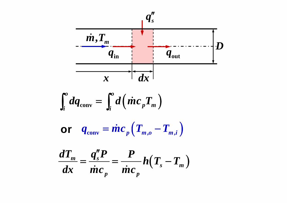
( )m ss m
p p
dT q P P h T Tdx mc mc
′′= = −
( )conv
o o
p mi idq d mc T=∫ ∫
or ( )conv , ,p m o m iq mc T T= −
x dx
Dinq
, mm Toutq
sq′′
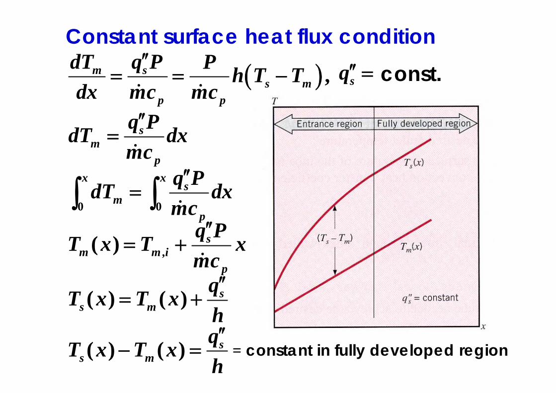
Constant surface heat flux condition
= constant in fully developed region
( ) ,m ss m
p p
dT q P P h T Tdx mc mc
′′= = − const.sq′′ =
sm
p
q PdT dxmc′′
=
0 0
x xs
mp
q PdT dxmc′′
=∫ ∫,( ) s
m m ip
q PT x T xmc′′
= +
( ) ( ) ss m
qT x T xh′′
= +
( ) ( ) ss m
qT x T xh′′
− =

Constant surface temperature condition
( )ms m
p
dT P h T Tdx mc
= − or m
m s p
dT P hdxT T mc
= −−
0 0
x xm
m s p
dT P hdxT T mc
= −−∫ ∫
( )0 0
lnxx
m sp
PT T hdxmc
⎡ ⎤− = −⎣ ⎦ ∫
0
1 x
xp p
Px Pxhdx hmc x mc
= − = −∫

,
( ) exps mx
s m i i p
T T x T Px hT T T mc
⎛ ⎞− Δ= = −⎜ ⎟⎜ ⎟− Δ ⎝ ⎠
For a tube of length L
,
,
s m o o
s m i i
T T TT T T− Δ
=− Δ
exp Lp
PL hmc
⎛ ⎞= −⎜ ⎟⎜ ⎟
⎝ ⎠

Log Mean Temperature Difference (LMTD)
Let , ,, ,i s m i o s m oT T T T T TΔ = − Δ = −
then ( )conv p i oq mc T T= Δ − Δ
,
,
exps m o oL
s m i i p
T T T PL hT T T mc
⎛ ⎞− Δ= = −⎜ ⎟⎜ ⎟− Δ ⎝ ⎠
lnln( / )
o LL p
p i i o
TPL PLhh mcmc T T T
Δ− = → =
Δ Δ Δ
( )conv , ,p m o m iq mc T T= −
( ) ( ), ,p s m i s m omc T T T T⎡ ⎤= − − −⎣ ⎦

( )conv p i oq mc T T= Δ − Δ
ln( / )L
pi o
PLhmcT T
=Δ Δ
( ) ( )conv ln /L
i oi o
PLhq T TT T
= Δ − ΔΔ Δ
( ) lmln /o i
L L so i
T TPLh h A TT T
Δ − Δ= ≡ Δ
Δ Δ
lm ln( / )o i
o i
T TTT T
Δ − ΔΔ =
Δ Δ
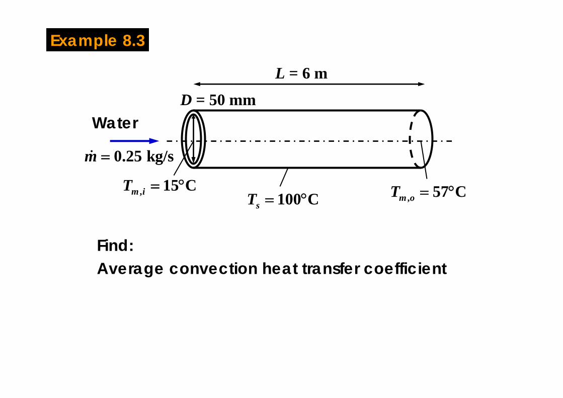
WaterD = 50 mm
L = 6 m
Example 8.3
Find: Average convection heat transfer coefficient
0.25 kg/sm =
, 15 Cm iT = °100 CsT = ° , 57 Cm oT = °

WaterD = 50 mm
L = 6 m
0.25 kg/sm =
, 15 Cm iT = °100 CsT = ° , 57 Cm oT = °
( )conv , ,p m o m iq mc T T= − lmshA T= Δ( ), ,
lm
p m o m i
s Tmc T
hT
A−
Δ→ =
( ) ( )( ) ( )
, ,
, ,lm 61.6 C
ln /s m o s m i
s m o s m i
T T T T
T T T TT
− − −= = °
⎡ ⎤− −⎣ ⎦Δ
( ) 20.25 4178 57 15756 W/m K
0.05 6 61.6h
π× × −
= =× × ×

in the cylindrical coordinate system (r,x)
for fully developed flow
Laminar Flow in Fully Developed RegionConvection Correlations
2
2
1T T T Tu v rx r r r r x
α⎡ ⎤∂ ∂ ∂ ∂ ∂⎛ ⎞+ = +⎜ ⎟⎢ ⎥∂ ∂ ∂ ∂ ∂⎝ ⎠⎣ ⎦
2
2
10 T T Tv u rx r r r x
α⎡ ⎤∂ ∂ ∂ ∂⎛ ⎞= → = +⎜ ⎟⎢ ⎥∂ ∂ ∂ ∂⎝ ⎠⎣ ⎦2
2( ) 2 1mo
ru r ur
⎛ ⎞= −⎜ ⎟
⎝ ⎠

Scaling , , ,u T r x2
2~ , ~ , ~ m om
o
u rT T T Tu r u xx r r r x r
α αα
∂ ∂ ∂ Δ Δ⎛ ⎞⎜ ⎟∂ ∂ ∂⎝ ⎠
2
/ ,Re Pr
o
o
m o o m o r
x rx x vxu r r v u rα α∗ = = =
,
, ,s
s m i m o
T T u ru rT T u r
θ ∗ ∗−= = =
−
Then,2 2
2 2 2 2
1 12 Re Pr
or
ux x r r rθ θ θ θ∗
∗ ∗ ∗ ∗ ∗
∂ ∂ ∂ ∂= + +
∂ ∂ ∂ ∂
When Re Pr Pe 100,or
= >T Tu rx r r r
α∂ ∂ ∂⎛ ⎞= ⎜ ⎟∂ ∂ ∂⎝ ⎠
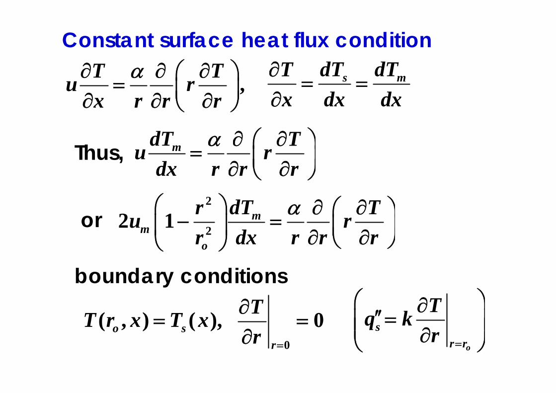
Constant surface heat flux condition
boundary conditions
s mdT dTTx dx dx
∂= =
∂
Thus, mdT Tu rdx r r r
α ∂ ∂⎛ ⎞= ⎜ ⎟∂ ∂⎝ ⎠
or 2
22 1 mm
o
dTr Tu rr dx r r r
α⎛ ⎞ ∂ ∂⎛ ⎞− =⎜ ⎟ ⎜ ⎟∂ ∂⎝ ⎠⎝ ⎠
( , ) ( ),o sT r x T x=0
0r
Tr =
∂=
∂o
sr r
Tq kr =
⎛ ⎞∂′′=⎜ ⎟⎜ ⎟∂⎝ ⎠
,T Tu rx r r r
α∂ ∂ ∂⎛ ⎞= ⎜ ⎟∂ ∂ ∂⎝ ⎠

from overall energy balance :
Integrating energy equation with boundary conditions
4m s s
p m p
dT q P qdx mc u Dcρ
′′ ′′= = = const.
4 22
2
2 3 1( , ) ( )16 16 4
m ms s
s
u dT r rT r x T x rdx rα
⎛ ⎞= − + −⎜ ⎟
⎝ ⎠
22 0
22 11( ) ( )96
or m mm s o
o m
u dTT x uTrdr T x rr u dxα
= = −∫11( )24
s os
q rT xk′′
= −

( ) 1124
s os s m
q rq h T T hk′′
′′ = − = ⋅
24 4811 11o
k khr D
= =
4811
Nu 4.364DhDk
= = =

Constant surface temperature condition
,s m
s m
T T dTTx T T dx
−∂=
∂ −s m
s m
T T dT Tu rT T dx r r r
α− ∂ ∂⎛ ⎞= ⎜ ⎟− ∂ ∂⎝ ⎠2
22 1 s mm
o s m
T T dTr Tu rr T T dx r r r
α⎛ ⎞ − ∂ ∂⎛ ⎞− =⎜ ⎟ ⎜ ⎟− ∂ ∂⎝ ⎠⎝ ⎠
Assume2
20
n
sn
ns m o
T T rCT T r
∞
=
⎛ ⎞−= ⎜ ⎟− ⎝ ⎠∑
( )2 20 0
0 2 2 2 4 2 221, 1.828397,4 (2 )n n nC C C C C
nλ λ
− −= = − = − = −
0 2.704364λ =
20Nu
23.657D
hDk
λ= = =

Example 8.4
absorber tube
concentrator
Conditions:
Find: 1) Length of tube L to achieve required heating2) Surface temperature Ts,o at the outlet section, x = L
Assumptions:1) Incompressible flow with constant properties2) Fully developed conditions at tube outlet
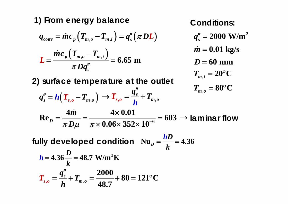
water22000 W/msq′′ =
0.01 kg/sm =
60 mmD =
, 20 Cm iT = °
, 80 Cm oT = °
( )s Lq Dπ′′=
1) From energy balance
2) surface temperature at the outlet
→ laminar flow
Nu 4.36DDk
h= =fully developed condition
24.36 48.7 W/m KDk
h = =
Conditions:22000 W/msq′′ =
0.01 kg/sm =60 mmD =
, 20 Cm iT = °
, 80 Cm oT = °
( )conv , ,p m o m iq mc T T= −
( ), , 6.65 mp m o m i
s
mc T TDq
Lπ
−= =
′′
( ), ,s os m oTq Th′′ = − ,,s
os o mqT Th′′
→ = +
6
4 4 0.01Re 6030.06 352 10D
mDπ μ π −
×= = =
× × ×
, ,2000 80 121 C48.7s o
sm oT
hT q′′
= + = + = °

Laminar Flow in the Entry RegionThermal entry length
Ts = constant,
properties at
( )( ) 2 / 3
0.0668 / Re PrNu 3.66
1 0.04 / Re PrD
D
D
D L
D L= +
⎡ ⎤+ ⎣ ⎦
lmNu ,D shD q hA Tk
= = Δ
( ), , / 2m m i m oT T T= +

Combined entry length(hydrodynamic + thermal)
properties at
Ts = constant
0.141/ 3Re PrNu 1.86/D
DsL Dμμ
⎛ ⎞⎛ ⎞= ⎜ ⎟⎜ ⎟⎝ ⎠ ⎝ ⎠
0.48 Pr 16,700
0.0044 9.75s
μμ
< <⎡ ⎤⎢ ⎥⎛ ⎞⎢ ⎥< <⎜ ⎟⎢ ⎥⎝ ⎠⎣ ⎦
( ), , / 2m m i m oT T T= +
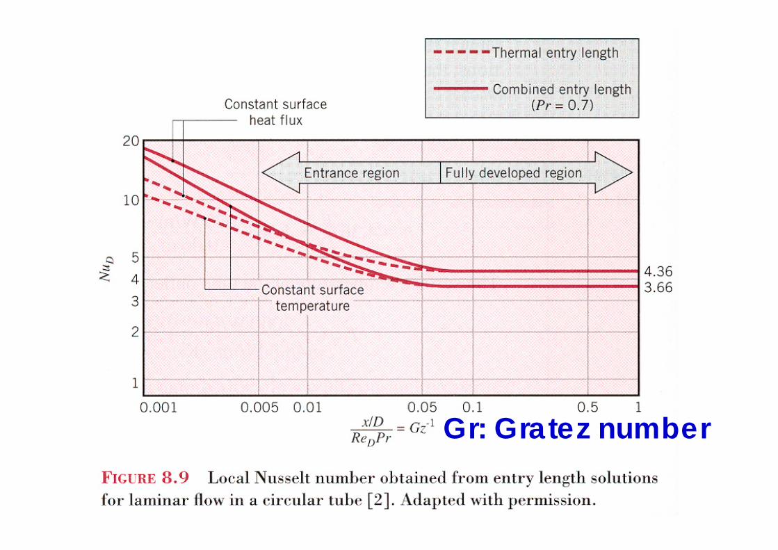
Gr: Gratez number
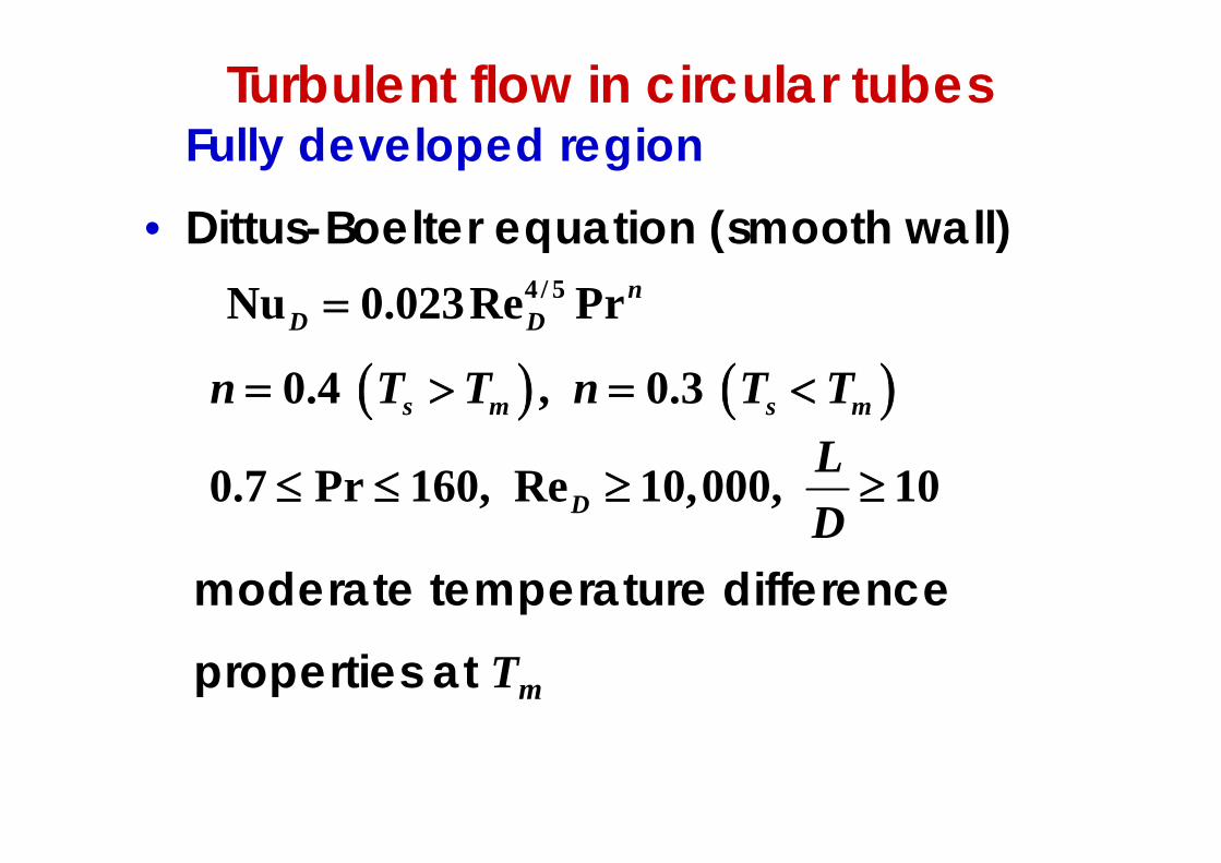
Turbulent flow in circular tubesFully developed region
• Dittus-Boelter equation (smooth wall)
moderate temperature differenceproperties at Tm
4 / 5Nu 0.023Re PrnD D=
( ) ( )0.4 , 0.3 s m s mn T T n T T= > = <
0.7 Pr 160, Re 10,000, 10DLD
≤ ≤ ≥ ≥
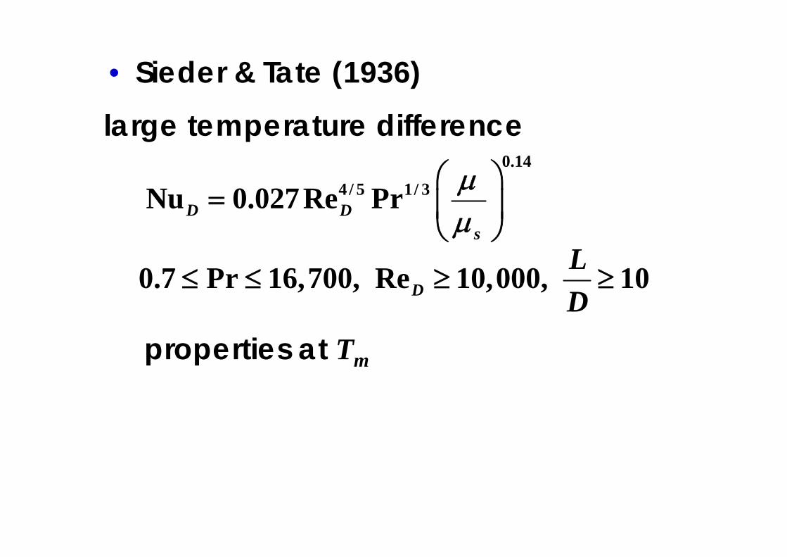
• Sieder & Tate (1936)
properties at Tm
large temperature difference0.14
4 / 5 1/ 3Nu 0.027Re PrD Ds
μμ
⎛ ⎞= ⎜ ⎟
⎝ ⎠
0.7 Pr 16,700, Re 10,000, 10DLD
≤ ≤ ≥ ≥
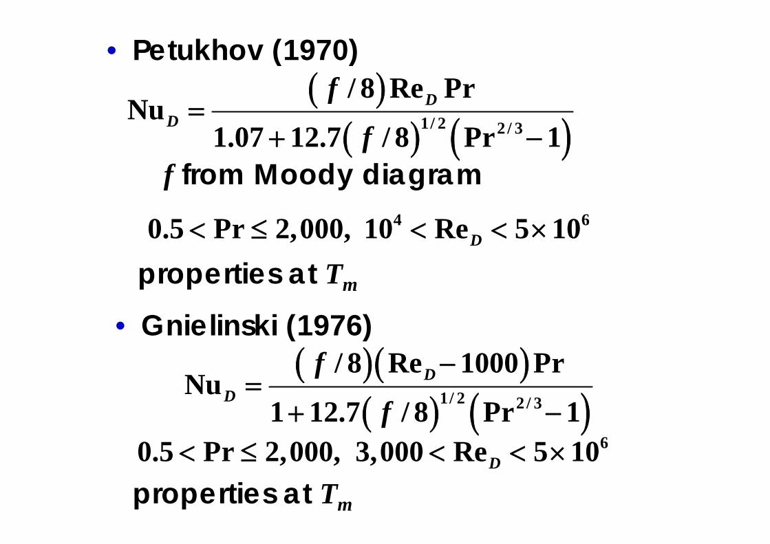
• Petukhov (1970)
f from Moody diagram
properties at Tm
( )( ) ( )1/ 2 2 / 3
/ 8 Re PrNu
1.07 12.7 / 8 Pr 1D
D
f
f=
+ −
4 60.5 Pr 2,000, 10 Re 5 10D< ≤ < < ×
• Gnielinski (1976)
properties at Tm
( )( )( ) ( )1/ 2 2 / 3
/ 8 Re 1000 PrNu
1 12.7 / 8 Pr 1D
D
f
f
−=
+ −60.5 Pr 2,000, 3,000 Re 5 10D< ≤ < < ×

Entry regionsince
For short tubes :
,fdNu NuD D= ( )fd10 / 60x D≤ ≤
,fd
Nu 1Nu ( / )
Dm
D
Cx D
= +
Liquid metals
constant
Ts = constant
fully developed turbulent flow0.827Nu 4.82 0.0185Pe ,D D= + sq′′ =
3 5
2 4
3.6 10 Re 9.05 1010 Pe 10
D
D
⎡ ⎤× < < ×⎢ ⎥< <⎣ ⎦
0.8Nu 5.0 0.025Pe ,D D= +

Hot air D = 0.15 m
L = 5 m
Cold ambient airx
Assumptions:1) Steady-state, constant properties, ideal gas behavior2) Uniform convection coefficient at outer surface of duct
Example 8.6
0.05 kg/sm =
,0 103 CmT = °
20 C, 6 W/m KoT h∞ = ° =
, 77 Cm LT = °
Find: 1) Heat loss from the duct over the length L, q[W]2) Heat flux and surface temperature Ts,L at x = L( )sq L′′
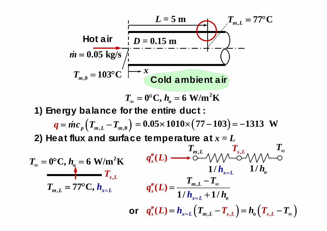
1) Energy balance for the entire duct :
2) Heat flux and surface temperature at x = L
Hot air D = 0.15 m
L = 5 m
Cold ambient airx
0.05 kg/sm =
,0 103 CmT = °
20 C, 6 W/m KoT h∞ = ° =
, 77 Cm LT = °
( ), ,0p m L mTq mc T= − ( )0.05 1010 77 103 1313 W= × × − = −
( )sq L′′,m LT ,s LT T∞
1/ x Lh = 1/ oh,
1 / /(
1)
x L
m L
os
T TL
hhq
=
∞−=
+′′
20 C, 6 W/m KoT h∞ = ° =
, 77 C, m L x LT h == °,s LT
( ) ( ), , ,( ) m L s Lx sL os Lq TL T Th h T= ∞′ =′ − = −or

turbulent flow
fully developed region
7
4 4 0.05Re 20,4040.15 208 10D
mDπ μ π −
×= = =
× × ×
/ 5 / 0.15 33.3 10L D = = >
4/ 5 0.3Nu 0.023Re Prx LD D
h Dk== = 57.9=
20.03Nu 57.9 11.6 W/m K0.15x L D D
h k= = = × =
Hence, , 277 0 304.5 W/m1/ 1/ 1 / 11.6 1/ 6.0
( ) m L
x L os
T Th
qh
L ∞
=
− −=
+′ = =
+′
( ) ( ), , ,( )s x L m L s L s LoT Tq L h T h T= ∞′′ = − = −
,,( ) 304.577 50.7 C
11.6s
m Lx L
s L TT q Lh =
′′= − = − = °

Convection Correlations: Noncircular Tube
hydraulic diameter :
Ac : flow cross-sectional area
P : wetted perimeter
4 ch
ADP
≡

Nusselt numbers and friction factors for fully developed laminar flow in tubes of different cross section

Concentric Tube Annulusinner wall :
outer wall :
Nusselt numbers
( ),i i s i mq h T T′′ = −
( ),o o s o mq h T T′′ = −
Nu , Nui h o hi o
h D h Dk k
≡ ≡
( )( )2 24 / 44 o ich o i
o i
D DAD D DP D D
π
π π
−= = = −
+
( ) ( )Nu NuNu , Nu
1 / 1 /ii oo
i oo i i i o oq q q qθ θ∗ ∗= =′′ ′′ ′′ ′′− −

For fully developed laminar flow1) One surface insulated and the
other at constant temperature

2) Uniform heat flux maintained at both surfaces
( ) ( )Nu NuNu , Nu
1 / 1 /ii oo
i oo i i i o oq q q qθ θ∗ ∗= =′′ ′′ ′′ ′′− −

Heat Transfer EnhancementInternal flow heat transfer enhancement schemes
Coil-spring wire insert Twisted tape insert
Longitudinal fins Helical ribs

Helically coiled tube and secondary flow
Recommended