HAL Id: tel-01127356https://tel.archives-ouvertes.fr/tel-01127356
Submitted on 7 Mar 2015
HAL is a multi-disciplinary open accessarchive for the deposit and dissemination of sci-entific research documents, whether they are pub-lished or not. The documents may come fromteaching and research institutions in France orabroad, or from public or private research centers.
L’archive ouverte pluridisciplinaire HAL, estdestinée au dépôt et à la diffusion de documentsscientifiques de niveau recherche, publiés ou non,émanant des établissements d’enseignement et derecherche français ou étrangers, des laboratoirespublics ou privés.
Interactions between rank and sparsity in penalizedestimation, and detection of structured objects
Pierre-André Savalle
To cite this version:Pierre-André Savalle. Interactions between rank and sparsity in penalized estimation, and detectionof structured objects. Other. Ecole Centrale Paris, 2014. English. NNT : 2014ECAP0051. tel-01127356

Ecole Centrale Paris
Thèse de Doctorat
Spécialité: Mathématiqes
Présentée par
Pierre-André Savalle
Interactions entre Rang et Parcimonie en
Estimation Pénalisée, et Détection
d’Objets Structurés
Soutenue le 21/10/2014 devant le jury composé de:
M. Alexandre D’ASPREMONT Ecole Normale Supérieure Rapporteur
M. Arnak DALALYAN CREST, ENSAE, Uni. Paris-Est Rapporteur
M. Gilles FAY Ecole Centrale Paris Directeur
M. Charles-Albert LEHALLE Capital Fund Management Examinateur
M. Guillaume OBOZINSKI Uni. Paris-Est, Ecole des Ponts Examinateur
M. Nicolas VAYATIS ENS Cachan Directeur
Thèse #: 2014ECAP0051


Contents
1 Introduction 15
1.1 Contributions: Interactions Between Rank and Sparsity . . . . . . . . . . . 17
1.1.1 Estimation of Sparse and Low Rank Matrices . . . . . . . . . . . . 17
1.1.2 Convex Localized Multiple Kernel Learning . . . . . . . . . . . . . 19
1.2 Contributions: Detection of Structured Objects . . . . . . . . . . . . . . . . 20
1.2.1 Detection of Correlations with Adaptive Sensing . . . . . . . . . . 21
1.2.2 Detection of Objects with High-dimensional CNN Features . . . . 23
I Interactions Between Rank and Sparsity in Penalized Estimation 27
2 Penalized Matrix Estimation 29
2.1 Introduction . . . . . . . . . . . . . . . . . . . . . . . . . . . . . . . . . . . 30
2.1.1 Linear Models: Generalization and Estimation . . . . . . . . . . . . 30
2.1.2 Occam’s Razor and Minimum Description Length . . . . . . . . . . 33
2.1.3 Priors and Penalized Estimation . . . . . . . . . . . . . . . . . . . . 34
2.1.4 Penalized Matrix Estimation . . . . . . . . . . . . . . . . . . . . . . 35
2.1.5 Penalized or Constrained? . . . . . . . . . . . . . . . . . . . . . . . 37
2.2 Sparsity . . . . . . . . . . . . . . . . . . . . . . . . . . . . . . . . . . . . . . 38
2.2.1 The ℓ0-norm . . . . . . . . . . . . . . . . . . . . . . . . . . . . . . 38
2.2.2 The ℓ1-norm . . . . . . . . . . . . . . . . . . . . . . . . . . . . . . 39
2.2.3 Elastic-net and Variations . . . . . . . . . . . . . . . . . . . . . . . 41
2.2.4 Other Regularizers . . . . . . . . . . . . . . . . . . . . . . . . . . . 42
2.3 Rank and Latent Factor Models . . . . . . . . . . . . . . . . . . . . . . . . . 43
2.3.1 The Rank . . . . . . . . . . . . . . . . . . . . . . . . . . . . . . . . 44
2.3.2 The Trace Norm . . . . . . . . . . . . . . . . . . . . . . . . . . . . 44
2.3.3 Nuclear and Atomic Norms . . . . . . . . . . . . . . . . . . . . . . 47
2.3.4 The Max Norm . . . . . . . . . . . . . . . . . . . . . . . . . . . . . 49
2.3.5 Other Heuristics and Open Problems . . . . . . . . . . . . . . . . . 50
2.4 Measuring Quality of Regularizers and Theoretical Results . . . . . . . . . 51
2.4.1 Estimation: Exact and Robust Recovery . . . . . . . . . . . . . . . 52
2.4.2 High-Dimensional Convex Sets and Gaussian Width . . . . . . . . 53
2.4.3 Optimality Conditions for Penalized Estimation . . . . . . . . . . . 54
2.4.4 Kinematic Formula and Statistical Dimension . . . . . . . . . . . . 57
2.4.5 Examples . . . . . . . . . . . . . . . . . . . . . . . . . . . . . . . . 58
2.4.6 Estimation with Non-gaussian Designs . . . . . . . . . . . . . . . . 60
3 Estimation of Sparse and Low Rank Matrices 63
3.1 Introduction . . . . . . . . . . . . . . . . . . . . . . . . . . . . . . . . . . . 64
3.1.1 Model . . . . . . . . . . . . . . . . . . . . . . . . . . . . . . . . . . 65
3.1.2 Main Examples . . . . . . . . . . . . . . . . . . . . . . . . . . . . . 65

4 CONTENTS
3.1.3 Outline . . . . . . . . . . . . . . . . . . . . . . . . . . . . . . . . . . 65
3.1.4 Notation . . . . . . . . . . . . . . . . . . . . . . . . . . . . . . . . . 66
3.2 Oracle Inequality . . . . . . . . . . . . . . . . . . . . . . . . . . . . . . . . 66
3.3 Generalization Error in Link Prediction . . . . . . . . . . . . . . . . . . . . 67
3.4 Algorithms . . . . . . . . . . . . . . . . . . . . . . . . . . . . . . . . . . . . 68
3.4.1 Proximal Operators . . . . . . . . . . . . . . . . . . . . . . . . . . . 68
3.4.2 Generalized Forward-backward Splitting . . . . . . . . . . . . . . . 69
3.4.3 Incremental Proximal Descent . . . . . . . . . . . . . . . . . . . . . 69
3.4.4 Positive Semi-denite Constraint . . . . . . . . . . . . . . . . . . . 70
3.5 Recovering Clusters . . . . . . . . . . . . . . . . . . . . . . . . . . . . . . . 70
3.6 Numerical Experiments . . . . . . . . . . . . . . . . . . . . . . . . . . . . . 71
3.6.1 Synthetic Data . . . . . . . . . . . . . . . . . . . . . . . . . . . . . 71
3.6.2 Real Data Sets . . . . . . . . . . . . . . . . . . . . . . . . . . . . . . 71
3.7 Discussion . . . . . . . . . . . . . . . . . . . . . . . . . . . . . . . . . . . . 73
3.7.1 Other Loss Functions . . . . . . . . . . . . . . . . . . . . . . . . . . 73
3.7.2 Optimization . . . . . . . . . . . . . . . . . . . . . . . . . . . . . . 74
3.7.3 Geometry . . . . . . . . . . . . . . . . . . . . . . . . . . . . . . . . 74
3.7.4 Factorization Methods . . . . . . . . . . . . . . . . . . . . . . . . . 75
3.8 Proofs . . . . . . . . . . . . . . . . . . . . . . . . . . . . . . . . . . . . . . . 78
3.8.1 Sketch of Proof of Proposition 13 . . . . . . . . . . . . . . . . . . . 78
3.8.2 Proof of Proposition 16 . . . . . . . . . . . . . . . . . . . . . . . . . 79
4 Convex Localized Multiple Kernel Learning 81
4.1 Introduction . . . . . . . . . . . . . . . . . . . . . . . . . . . . . . . . . . . 82
4.1.1 Linear MKL . . . . . . . . . . . . . . . . . . . . . . . . . . . . . . . 82
4.1.2 Hinge Loss Aggregation . . . . . . . . . . . . . . . . . . . . . . . . 83
4.1.3 Related Work . . . . . . . . . . . . . . . . . . . . . . . . . . . . . . 84
4.1.4 Outline . . . . . . . . . . . . . . . . . . . . . . . . . . . . . . . . . . 86
4.1.5 Notation . . . . . . . . . . . . . . . . . . . . . . . . . . . . . . . . . 86
4.2 Generalized Hinge Losses . . . . . . . . . . . . . . . . . . . . . . . . . . . . 86
4.2.1 Representer Theorem . . . . . . . . . . . . . . . . . . . . . . . . . . 88
4.2.2 Universal Consistency . . . . . . . . . . . . . . . . . . . . . . . . . 89
4.3 ℓp-norm Aggregation of Hinge Losses . . . . . . . . . . . . . . . . . . . . . 91
4.3.1 Dual Problem . . . . . . . . . . . . . . . . . . . . . . . . . . . . . . 91
4.3.2 Regularization . . . . . . . . . . . . . . . . . . . . . . . . . . . . . . 93
4.3.3 Link Functions . . . . . . . . . . . . . . . . . . . . . . . . . . . . . 94
4.4 Experiments . . . . . . . . . . . . . . . . . . . . . . . . . . . . . . . . . . . 94
4.4.1 UCI Datasets . . . . . . . . . . . . . . . . . . . . . . . . . . . . . . 95
4.4.2 Image Classication . . . . . . . . . . . . . . . . . . . . . . . . . . 96
4.5 Discussion . . . . . . . . . . . . . . . . . . . . . . . . . . . . . . . . . . . . 97
4.6 Proofs . . . . . . . . . . . . . . . . . . . . . . . . . . . . . . . . . . . . . . . 98
4.6.1 Proof of Lemma 2 . . . . . . . . . . . . . . . . . . . . . . . . . . . . 98
4.6.2 Proof of Lemma 3 . . . . . . . . . . . . . . . . . . . . . . . . . . . . 98
4.6.3 Proof of Lemma 4 . . . . . . . . . . . . . . . . . . . . . . . . . . . . 99
4.6.4 Proof of Lemma 5 . . . . . . . . . . . . . . . . . . . . . . . . . . . . 99
4.6.5 Proof of Theorem 3 . . . . . . . . . . . . . . . . . . . . . . . . . . . 100

CONTENTS 5
II Detection of Structured Objects 101
5 Detection of Correlations with Adaptive Sensing 103
5.1 Introduction . . . . . . . . . . . . . . . . . . . . . . . . . . . . . . . . . . . 104
5.1.1 Model . . . . . . . . . . . . . . . . . . . . . . . . . . . . . . . . . . 104
5.1.2 Adaptive vs. Non-adaptive Sensing and Testing . . . . . . . . . . . 105
5.1.3 Uniform Sensing and Testing . . . . . . . . . . . . . . . . . . . . . 107
5.1.4 Related Work . . . . . . . . . . . . . . . . . . . . . . . . . . . . . . 108
5.1.5 Outline . . . . . . . . . . . . . . . . . . . . . . . . . . . . . . . . . . 109
5.1.6 Notation . . . . . . . . . . . . . . . . . . . . . . . . . . . . . . . . . 109
5.2 Lower Bounds . . . . . . . . . . . . . . . . . . . . . . . . . . . . . . . . . . 110
5.3 Adaptive Tests . . . . . . . . . . . . . . . . . . . . . . . . . . . . . . . . . . 113
5.3.1 Sequential Thresholding . . . . . . . . . . . . . . . . . . . . . . . . 113
5.3.2 The Case of k-intervals . . . . . . . . . . . . . . . . . . . . . . . . . 115
5.3.3 The Case of k-sets: Randomized Subsampling . . . . . . . . . . . . 118
5.4 Unnormalized Correlation Model . . . . . . . . . . . . . . . . . . . . . . . 120
5.4.1 Model and Extensions of Previous Results . . . . . . . . . . . . . . 120
5.4.2 The Case of k-sets . . . . . . . . . . . . . . . . . . . . . . . . . . . 120
5.5 Discussion . . . . . . . . . . . . . . . . . . . . . . . . . . . . . . . . . . . . 122
5.6 Proofs . . . . . . . . . . . . . . . . . . . . . . . . . . . . . . . . . . . . . . . 124
5.6.1 Inequalities and KL Divergences . . . . . . . . . . . . . . . . . . . 124
5.6.2 Proof of Bound on KL Divergence . . . . . . . . . . . . . . . . . . . 125
5.6.3 Proof of Proposition 18 . . . . . . . . . . . . . . . . . . . . . . . . . 125
5.6.4 Proof of Proposition 19 . . . . . . . . . . . . . . . . . . . . . . . . . 126
5.7 Appendix: Extensions to Unnormalized Model . . . . . . . . . . . . . . . . 127
5.7.1 Uniform (non-adaptive) Lower Bound . . . . . . . . . . . . . . . . 127
5.7.2 Uniform (non-adaptive) Upper Bound . . . . . . . . . . . . . . . . 127
5.7.3 KL Divergences . . . . . . . . . . . . . . . . . . . . . . . . . . . . . 127
6 Detection of Objects with CNN Features 131
6.1 Introduction . . . . . . . . . . . . . . . . . . . . . . . . . . . . . . . . . . . 132
6.2 Detection with DPMs . . . . . . . . . . . . . . . . . . . . . . . . . . . . . . 133
6.2.1 Detection Task . . . . . . . . . . . . . . . . . . . . . . . . . . . . . 133
6.2.2 Deformable Part Models . . . . . . . . . . . . . . . . . . . . . . . . 133
6.3 Integrating Convolutional Features into DPMs . . . . . . . . . . . . . . . . 135
6.3.1 The Alexnet Network Structure . . . . . . . . . . . . . . . . . . . . 135
6.3.2 Prior Work . . . . . . . . . . . . . . . . . . . . . . . . . . . . . . . 136
6.3.3 Using CNN Layer 5 Features in DPMs . . . . . . . . . . . . . . . . 137
6.4 Results on Pascal VOC 2007 . . . . . . . . . . . . . . . . . . . . . . . . . . 138
Bibliography 141


Résumé
Cette thèse est organisée en deux parties indépendantes. La première partie s’intéresse à
l’estimation convexe de matrice en prenant en compte à la fois la parcimonie et le rang.
Dans le contexte de graphes avec une structure de communautés, on suppose souvent
que la matrice d’adjacence sous-jacente est diagonale par blocs dans une base appropriée.
Cependant, de tels graphes possèdent généralement une matrice d’adjacente qui est aussi
parcimonieuse, ce qui suggère que combiner parcimonie et rang puisse permettre de mod-
éliser ce type d’objet de manière plus ne. Nous proposons et étudions ainsi une pénalité
convexe pour promouvoir parcimonie et rang faible simultanément. Même si l’hypothèse
de rang faible permet de diminuer le sur-apprentissage en diminuant la capacité d’un mod-
èle matriciel, il peut être souhaitable lorsque susamment de données sont disponibles
de ne pas introduire une telle hypothèse. Nous étudions un exemple dans le contexte
multiple kernel learning localisé, où nous proposons une famille de méthodes á vaste-
marge convexes et accompagnées d’une analyse théorique. La deuxième partie de cette
thèse s’intéresse à des problèmes de détection d’objets ou de signaux structurés. Dans un
premier temps, nous considérons un problème de test statistique, pour des modèles où
l’alternative correspond à des capteurs émettant des signaux corrélés. Contrairement à la
littérature traditionnelle, nous considérons des procédures de test séquentielles, et nous
établissons que de telles procédures permettent de détecter des corrélations signicative-
ment plus faibles que les méthodes traditionnelles. Dans un second temps, nous consid-
érons le problème de localiser des objets dans des images. En s’appuyant sur de récents
résultats en apprentissage de représentation pour des problèmes similaires, nous intégrons
des features de grande dimension issues de réseaux de neurones convolutionnels dans les
modèles déformables traditionnellement utilisés pour ce type de problème. Nous démon-
trons expérimentalement que ce type d’approche permet de diminuer signicativement le
taux d’erreur de ces modèles.


Abstract
This thesis is organized in two independent parts. The rst part focused on convex matrix
estimation problems, where both rank and sparsity are taken into account simultaneously.
In the context of graphs with community structures, a common assumption is that the
underlying adjacency matrices are block-diagonal in an appropriate basis. However, these
types of graphs are usually far from complete, and their adjacency representations are thus
also inherently sparse. This suggests that combining the sparse hypothesis and the low
rank hypothesis may allow tomore accurately model such objects. To this end, we propose
and analyze a convex penalty to promote low rank and high sparsity simultaneously. Al-
though the low rank hypothesis allows to reduce over-tting by decreasing the modeling
capacity of a matrix model, the opposite may be desirable when enough data is available.
We study such an example in the context of localized multiple kernel learning, which ex-
tends multiple kernel learning by allowing each of the kernels to select dierent support
vectors. In this framework, multiple kernel learning corresponds to a rank one estimator,
while higher-rank estimators have been observed to increase generalization performance.
We propose a novel family of large-margin methods for this problem that, unlike previ-
ous methods, are both convex and theoretically grounded. The second part of the thesis
is about detection of objects or signals which exhibit combinatorial structures, and we
present two such problems. First, we consider detection in the statistical hypothesis test-
ing sense, in models where anomalous signals correspond to correlated values at dierent
sensors. In most existing work, detection procedures are provided with a full sample of
all the sensors. However, the experimenter may have the capacity to make targeted mea-
surements in an on-line and adaptive manner, and we investigate such adaptive sensing
procedures. Finally, we consider the task of identifying and localizing objects in images.
This is an important problem in computer vision, where hand-crafted features are usually
used. Following recent successes in learning ad-hoc representations for similar problems,
we integrate the method of deformable part models with high-dimensional features from
convolutional neural networks, and shows that this signicantly decreases the error rates
of existing part-based models.


Acknowledgements
First, I would like to thank Gilles and Nicolas, for never loosing faith that this thesis
would lead somewhere, providing me with a much coveted mix of safety and freedom. I
hope that this is only the beginning of manymore adventures together. My deepest thanks
to Alexandre d’Aspremont and Arnak Dalalyan for doing me the honor of agreeing to
review this thesis. I am also grateful to Charles-Albert Lehalle and Guillaume Obozinski,
for participating in my thesis committee, and for taking interest in my work. I am more
than humbled to have you all on my committee.
I also would like to thank everyone I have had the opportunity to work with these last
three years: all my thanks to Emile, for so many heated discussions and good moments;
to Gábor, for welcoming me so warmly in Barcelona, and showing me how blissful riding
the roller coaster of research can be; to Iasonas, who swore never again to stay up late
on deadlines, and yet is still trying out the next idea around the clock; to Rui, who knows
more about parisian rooftops than I might ever do. My thoughts and my gratitude also
go to everyone that has supported me in these last years; to everyone I’ve crossed path
with at CMLA; to Rémy, who never backs away from a ght with a taco or a mathematical
conjecture; to everyone at MAS for scores of unforgettable moments, and most particu-
larly to Alex, Benjamin, Benoit, Blandine, Charlotte, Marion, Ludovic, Gautier; to Annie,
Micheline, Sylvie and Virginie; to Nikos, for consistently reminding me of upcoming dead-
lines, and consistently believing in me; to Benoit, who has more ideas by the minute than
any reasonable person has by the day, and who has been a constant support throughout
these three years; to Jérémy, my sparing partner, who is feared by wavelet-sparse signals
and bacon toppings across the entire universe; to all my friends and my family, and, most
importantly, to Hélène and my parents.
Finally, I want to dedicate this work to Ben Taskar, who is missed by all more than my
words can clumsily express.


Notation
General
[d] 1, . . . ,ddiam(X) Diameter of set X in Euclidean norm p. 54
ΠC Projection operator onto the convex set C p. 57
diag(M) Vector of diagonal elements of matrixMX Y Hadamard product of X and Y p. 36
M+ Componentwise positive part of matrixMTr(M) Trace of matrixM p. 45
M 0 MatrixM is positive semi-denite p. 45
kerM Kernel of matrixM p. 52
1 All ones vector p. 30
1[C] Zero-one indicator function of condition C p. 32
δX Barrier indicator function of set X p. 40
convX Convex hull of set X p. 42
coneX Conical hull of set X p. 54
f ⋆ Convex conjugate of function f p. 40
f ⋆⋆ Convex biconjugate of function f p. 40
KL Kullback-Leibler divergence p. 110
Matrix Norms and Balls
‖ · ‖⋆ Dual norm to ‖ · ‖ p. 47
‖M‖0 = cardMi,j , 0| ℓ0-norm of matrixM
‖M‖p =[∑
i,j |Mi,j |p]1/p
ℓp-norm of matrixM
‖M‖1 =∑i,j |Mi,j | ℓ1-norm of matrixM
‖M‖F =√∑
i,jM2i,j Frobenius norm of matrixM
‖M‖∞ =max |Mi,j | ℓ∞-norm of matrixM‖M‖op = supx : ‖x‖2=1 ‖Mx‖2 Operator norm of matrixM
‖M‖∗ Trace norm of matrixM p. 45
‖M‖max Max norm of matrixM p. 49
BΩ Unit ball of norm Ω p. 34
SΩ Unit sphere of norm Ω p. 34
w(C) Gaussian width of set C p. 53
∆(C) Statistical dimension of set C p. 57
N (X,‖.‖,ε) ε-covering number of X with respect to norm ‖.‖ p. 89
H(X,‖.‖,ε) Metric entropy (logarithm of covering number) p. 89


1Introduction
“The most exciting phrase to hear inscience, the one that heralds newdiscoveries, is not ’Eureka!’ (I found it!) but’That’s funny ...’
— Isaac Asimov
The cognitive process in the brain can be simplied down to two processes around
which thinking is structured: induction and deduction. In induction, we build new mental
models from observations, while in deduction, we use these mental models to make pre-
dictions and take actions. These two phases are continuously alternating, and although
deduction is easy, induction is fundamentally harder and ill-dened. At a high-level, many
methods in machine learning can be understood as such continuously alternating phases
of induction and deduction. This is particularly visible in methods which aim at learning a
feature representation from the data, such as in dictionary learning, where induction cor-
responds to the estimation of codewords, and deduction to the coding problem. Convex
methods correspond to a rather simplied modeling environment where induction and
deduction are actually done jointly through some well-grounded optimization algorithm.
Although the cognitive process is a highly non-convex process, simple mental models can
be useful to get some initial insight on a problem or a concept at a moderate cost. Similarly,
convex methods have proven dramatically useful to approach many statistical modeling
and learning problems, and we believe that advancing the state of knowledge in what can
be eectively handled with this type of methods is of utmost interest. This does not mean,
however, that non-convex methods should be avoided, and many such methods have re-
cently proven very eective at achieving state of the art results in a variety of problems.
Instead, we believe that the classical debate of which of convex or non-convex methods
are best is actually moot, and that these two classes correspond to largely dierent trade-
os. If one were to draw a cartoon picture, convex methods are usually associated with
lower computational and modeling eorts, and can often be used to quickly gain signi-
cant insight on a given problem. Non-convex methods are generally signicantly heavier
to deploy and require an arguably more hands-on expertise, but have repeatedly proven
eective at going further than convex methods in many learning and pattern recognition
tasks.
This thesis is organized in two independent parts. This chapter summarizes our results
and contributions. The rst part of the thesis is on convex estimation problems, with
an emphasis on combining classical hypotheses usually handled in isolation for matrix

16 CHAPTER 1. INTRODUCTION
estimation. We consider how objects such as graphswith community structure, covariance
matrices or mixtures of kernel machines can be modeled in a convex framework, and we
focus in particular on models involving rank and sparsity hypotheses. The second part of
the thesis is on two examples of detection problems, where objects or signals to be detected
have some type of combinatorial structure. This departs largely from convex models, as
we consider both information-theoretically optimal procedures and numerically successful
methods which are highly non-convex.
1.1. CONTRIBUTIONS: INTERACTIONS BETWEEN RANK AND SPARSITY 17
1.1 Contributions: Interactions Between Rank and Sparsity
The rst part of this thesis is focused on penalized estimation problems for regression and
classication. More specically, we consider convex problems for estimating matrices.
A key element which dierentiate this problem from standard high dimensional vector
estimation is that dierent structural assumptions can be formulated in this context: al-
though sparsity hypotheses can be transposed from the vector case, genuinely dierent
hypotheses can be formulated, such as the low rank hypothesis.
The concepts of sparsity and of low rank have been central in statistics and machine
learning in the last decade, and have been at the source of numerous successes. At the
core of the sparsity hypothesis lies the idea that the data may be well modeled by a limited
number of features or variables, and that performing variable selection may increase the
predictive performance (Mallat, 1999; Bühlmann and Van De Geer, 2011). The low rank
hypothesis is at the source of a variety of models usually referred to as latent factor models,
which are also widely recognized as eective in practice, such as in clustering (Shahnaz
et al., 2006), recommender systems (Koren, 2008), or blind source separation (Cichocki
et al., 2009).
Chapter 2 is dedicated to reviewing the ideas underlying sparsity and of low rank
models. We also briey retrace the history of penalized estimation, and present general
geometric tools which can be used to study the estimation performance of a large array
of convex penalties from a theoretical point of view. In Chapter 3 and Chapter 4, we
consider two matrix estimation problems, where both rank and sparsity are taken into
account simultaneously, albeit in dierent ways. In the following, we present a preview
of the results from these two works.
1.1.1 Estimation of Sparse and Low Rank Matrices
In recent years, the notion of sparsity for vectors has been transposed into the concept of
low rank matrices, and this latter hypothesis has opened up the way to numerous achieve-
ments (Srebro, 2004; Cai et al., 2008). In Chapter 3, we argue that being low rank is not
only an equivalent of sparsity for matrices but also that low rank and sparsity can actually
be seen as two orthogonal concepts. The underlying structure we have in mind is that of a
block diagonal matrix. This situation occurs for instance in covariance matrix estimation
in the case of groups of highly correlated variables or when clustering social graphs.
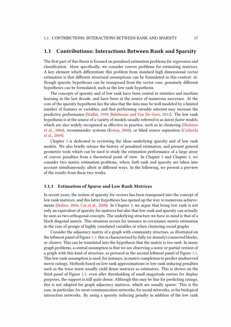
Consider the adjacency matrix of a graph with community structure, as illustrated on
the leftmost panel of Figure 1.1: this is characterized by fully (or densely) connected blocks,
or clusters. This can be translated into the hypothesis that the matrix is low rank. In many
graph problems, a central assumption is that we are observing a noisy or partial version of
a graph with this kind of structure, as pictured in the second leftmost panel of Figure 1.1.
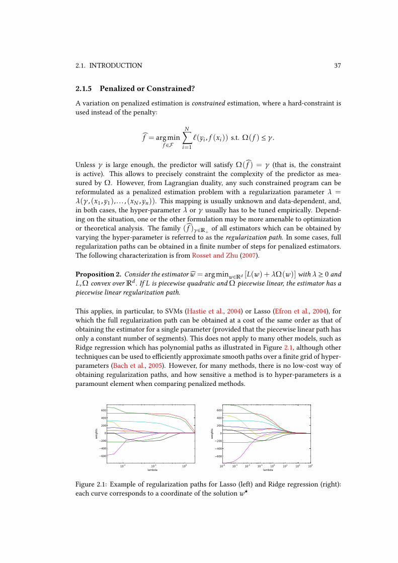
This low rank assumption is used, for instance, in matrix completion to predict unobserved
movie ratings. Methods based on low rank approximations or low rank inducing penalties
such as the trace norm usually yield dense matrices as estimators. This is shown on the
third panel of Figure 1.1: even after thresholding of small magnitude entries for display
purposes, the support is still quite dense. Although this may be ne for predicting ratings,
this is not adapted for graph adjacency matrices, which are usually sparse. This is the
case, in particular, for most communication networks, for social networks, or for biological
interaction networks. By using a sparsity inducing penalty in addition of the low rank

18 CHAPTER 1. INTRODUCTION
Figure 1.1: Adjacency matrix with community structure, sparse regularization, low rank
regularization, and sparse low rank regularization
inducing penalty, we obtain the support shown on the rightmost panel of Figure 1.1, which
is a much better recovery of the original graph structure.
The problem of leveraging both types of structures at the same time is largely dierent
from demixing or decomposition problems (Amelunxen et al., 2013) such as Robust PCA
(Candès et al., 2011; Chandrasekaran et al., 2011), where the objective is to recover a sparse
matrix S ∈ Rd1×d2 and a low rank matrix L ∈ Rd1×d2 from the knowledge of their sum
X = L+ S only. For this type of problem, objective functions usually take the form of
an inmal convolution (Rockafellar, 1997) of penalties (Agarwal et al., 2012). On the other
hand, we consider here a single matrix that is simultaneously sparse and low rank.
Contributions. We propose a novel convex penalty to encourage solutions that achieve
a tradeo between low rank and high sparsity. The penalty is based on a linear combina-
tion of the classical surrogates, the matrix ℓ1-norm, and the trace norm : for a matrix
W ∈Rd×d , the penalty is
γ‖W ‖1+ (1−γ)‖W ‖∗.We derive oracle inequalities for penalized estimation using this penalty.
Proposition 1. LetW ⋆ ∈Rd×d and A =W ⋆ + ǫ with ǫ ∈Rd×d having i.i.d. entries withzero mean. Assume for some α ∈ [0,1] that τ ≥ 2α‖ǫ‖op and γ ≥ 2(1−α)‖ǫ‖∞. Let
W = argminW∈Rd×d
[‖W −A‖2F + γ‖W ‖1+ τ‖W ‖∗
].
Then,
‖W −W ⋆‖2F ≤ infW∈Rd×d
[‖W −W ⋆‖2F + 2γ‖W ‖1+ 2τ‖W ‖∗
],
‖W −W ⋆‖2F ≤[2γ‖W ⋆‖1+ 2τ‖W ⋆‖∗
]∧
[γ√‖W ⋆‖0+ τ
√rank(W ⋆)
√2+ 1
2
]2.
This is extended in Proposition 13 to constrained optimization (for instance over the cone
of semi-denite positive matrices), and generalizes previous sharp bounds for Lasso or
trace norm regression (Koltchinskii et al., 2011a). Combined with proper choices of reg-
ularization parameters that we discuss, this allows to control the prediction error. Using
proximal methods, we demonstrate the benets of combining these two hypotheses both
on synthetic data, and on real data such as protein interaction data and social networks.
This chapter is an extended version of a paper with Emile Richard and Nicolas Vayatis
which has appeared in the proceedings of ICML (Richard et al., 2012).

1.1. CONTRIBUTIONS: INTERACTIONS BETWEEN RANK AND SPARSITY 19
Future directions. We propose a convex relaxation to the intersection of the two classi-
cal manifolds that are sparse matrices and low rank matrices. However, it may well be that
there are some more interesting joint measure of rank and sparsity to relax when model-
ing the type of data we are interested in. We discuss possible directions based on matrix
factorizations and atomic norms in Section 3.7. More generally, the following problem
appears of interest: how can multiple priors on a model be combined to estimate the model
with fewer observations, and for what prior structures is this a signicant improvement over
using a single prior? For instance, Kamal and Vandergheynst (2013) consider combining
rank and sparsity, but in dierent bases. An interesting direction to tackle this problem
could be learning to combine such priors, as done with kernels and Hilbert space metrics
in multiple kernel learning.
1.1.2 Convex Localized Multiple Kernel Learning
The low rank hypothesis allows to decrease the modeling capacity of a matrix model,
which may be helpful in a high-dimensional setting to avoid over-tting. In other set-
tings, however, the opposite may be desirable: more complex models may allow to obtain
better generalization performance if enough data is available. We consider in Chapter 4
such an examples, in the context of localized multiple kernel learning. Kernel-based meth-
ods such as SVMs are very eective tools for classication and regression. In addition to
good empirical performance in a wide range of situations, these method and backed by a
strong theoretical background (Steinwart and Christmann, 2008), as well as mature algo-
rithms (Platt, 1999) and implementations (Chang and Lin, 2011). The kernel is traditionally
either selected from generic parametric o-the-shelf kernels (e.g., Gaussian or polynomial)
using some sort of cross-validation, or hand-crafted by domain specic experts through an
expensive empirical process. Multiple kernel learning (MKL) has been proposed to allevi-
ate part of this expensive model selection problem (Lanckriet et al., 2002; Bach et al., 2004;
Gönen and Alpaydın, 2011). In MKL, the SVM formulation is modied to jointly learn a
classier and linear combination weights for a set K1, . . . ,KM of kernels. This results in
classiers of the form
f (x) =N∑
i=1
yiαi
M∑
m=1
smKm(xi ,x)
︸ ︷︷ ︸kernel is a mixture of kernels
,
where α ∈ RN and s1, . . . ,sM ∈ R+ are to be both learned at the same time. In the wake
of the success of MKL, there has been recent interest in combining kernels in a localized
or data-dependent way (Bi et al., 2004; Gönen and Alpaydin, 2008; Cao et al., 2009; Gehler
and Nowozin, 2009), as opposed to more traditional linear combinations where all the
kernels must agree on a common set of support vectors. By allowing each kernel to select
separate and possibly dierent support vectors, these may be more relevant with respect
to the information encoded by the kernels. These approaches are referred to as either
localized, or data-dependent multiple kernel learning.
In the chapter, we focus on fully nonparametric localized MKL classiers of the form
f (x) =N∑
i=1
M∑
m=1
yiαi,mKm(xi ,x),
20 CHAPTER 1. INTRODUCTION
where α ∈RN×M is a matrix. While the solution to the linear MKL problem can be written
in this form with rank(α) = 1, we are interested in higher rank solutions which exhibit
localization, in the sense that the relative weights of the kernels vary depending on the
support vectors. Informally, this corresponds to a kernel combination that is dierent in
dierent regions of the feature space. Previous methods are either non-convex, are not
large margin methods, or consider only parametric models for α.
Contributions. We propose a family of large-margin methods that are both convex and
theoretically grounded for combining kernels in a data-dependent manner, based on ag-
gregating hinge losses over each of the kernels. For p ∈ [1,∞], we consider large margin
programs of the form
minω=(ω1,...,ωM )∈H
1
2
M∑
m=1
‖ωm‖22+CN∑
i=1
M∑
m=1
(1− yi〈ω1,φm(xi)〉)p+
1/p,
where φ1, . . . ,φM are the feature mappings associated to the kernels. This allows through
p to adjust the amount of coupling between the kernels. When p = ∞, kernels are the
most tightly coupled, while when p = 1, the method amounts to averaging the decisions
of independently trained SVMs. We show that classiers dened from these programs
(and actually more general aggregations) are universally consistent, and we consider the
question of whether intermediate levels of coupling can be benecial in practice.
We evaluate these methods on real data, including both UCI datasets, and image classi-
cation tasks from computer vision. Our experimental validation includes multiple meth-
ods which have not been previously compared, although they address a similar question.
Our experimental validation shows that p = 1 (i.e., averaging the decisions of independent
SVMs) is superior to any other value of p, but also to standard MKL and previously intro-
duced methods for localized MKL. In addition of being by far the simplest and cheapest to
implement and run, this yields the best (or close to the best) classication accuracy in all of
our benchmarks. Similarly to how the simple average kernel often achieves performances
comparable to that of MKL (Gehler and Nowozin, 2009), this suggests that straightforward
methods may achieve close to state-of-the-art accuracies for localized MKL as well. This
chapter is joint work with Antoine Poliakov, and has been submitted.
1.2 Contributions: Detection of Structured Objects
Detection problems are a wide and pervasive class of problem, where the high-level goal
is to detect expected or unexpected patterns from observations and data. This type of
problem diers signicantly from matrix estimation problems as presented in the rst
part of this thesis, in that themodels and structures involved are usually radically dierent.
In the second part of this thesis, we consider two types of detection problems involving
structured target objects, from statistical hypothesis testing and computer vision.
In the rst problem, we consider detection in the statistical hypothesis testing sense:
we want to known whether there is some anomalous signal, but we do not seek to identify
precisely where. We characterize the minimax risk in dierent models where anomalous
signals correspond to correlated values at dierent sensors. In the second problem, we
consider the more applied task of identifying dierent types of real-world objects in im-
ages. The detection terminology has a dierent meaning here than in statistical testing:

1.2. CONTRIBUTIONS: DETECTION OF STRUCTURED OBJECTS 21
the objective is to precisely localizing where in the image these object are. We integrate
the method of deformable part models with high-dimensional features from convolutional
neural networks, and shows that this signicantly decreases the error rate of DPMs.
1.2.1 Detection of Correlations with Adaptive Sensing
The rst detection problem that we consider is a statistical hypothesis testing problem.
Given multiple observations from a Gaussian multivariate distribution, we want to test
whether the corresponding covariance matrix is diagonal against non-diagonal alterna-
tives. More precisely, we consider a testing problem over a Gaussian vectorU ∈Rn, where
under the alternative hypothesis, there exists an unknown subset S of 1, . . . ,n such that
the corresponding components are positively correlated with strength ρ ∈]0,1[, while theothers are independent.
This can be interpreted as an anomaly detection problem: picture a spatially arranged
array of sensors. In the normal regime, signals at each of the sensors consists only of
zero-mean uncorrelated Gaussian noise. In the anomalous regime, some of the sensors
instead have correlated signals. This has to be distinguished from many classical anomaly
detection problems where one assume that the anomaly is characterized by an elevated
signal mean at some of the sensors. In the model that we consider, anomalies cannot
be detected by looking at sensors in isolation, but only when considering correlations
between multiple sensors.
The models that we consider are very similar to the rank one spiked covariance model,
which has been associated in recent years to sparse PCA (Johnstone and Lu, 2009; Berthet
and Rigollet, 2013; Cai et al., 2013). We focus on detection of positive correlations (Arias-
Castro et al., 2012, 2014), and we consider the sparse regime where only a relatively small
number of the n components are correlated, if any. The subset S can be any subset of size
of a known size k (which we refer to as the k-sets problem), or may have additional struc-
ture known to the experimenter. For instance, it can consists of k contiguous coordinatesin 1, . . . ,n, in which case one expects that detection will be easier due to this extra infor-
mation. This last setting is referred to as the k-intervals problem, and can be generalized
for instance to rectangles i0, . . . , i0 + k1 − 1 × j0, . . . , j0 + k2 − 1 with k1k2 = k, whenthe n coordinates are arranged spatially on a two dimensional grid 1, . . . ,n1 × 1, . . . ,n2with n1n2 = n.
In the litterature (Hero and Rajaratnam, 2012; Arias-Castro et al., 2014, 2012; Berthet
and Rigollet, 2013; Cai et al., 2013), this problem or related problems have been analyzed
under uniform sensing, where i.i.d. draws U1, . . . ,Um ∈ Rn of the Gaussian vector are
available. Our approach deviates from this in that we consider an adaptive sensing or se-
quential experimental design setting. More precisely, data is collected in a sequential and
adaptive way, where data collected at earlier stages informs the collection of data in future
stages. In particular, the experimenter may choose to acquire only a subset of the coor-
dinates from the Gaussian vector. In the previous sensor array illustration, a cost may be
associated to obtaining a measurement from a sensor, and the experimenter may choose
to activate only specic subsets of sensors. This is illustrated in Figure 1.2. Here, coor-
dinates 1, . . . ,n are laid out according to a grid. The set of correlated coordinates is a
convex shape, and these are shown in red. These coordinates form a clique in the graph
of correlations, and this is shown through light red edges. At every step, the experimenter
selects coordinates to be sensed, and these are shown circled. At the rst step, the exper-

22 CHAPTER 1. INTRODUCTION
imenter samples all the coordinates, while at the two subsequent steps, the experimenter
reduced the amount of coordinates sampled. This illustrates an important point: we only
Figure 1.2: Adaptive sensing over a two dimensional grid of sensors
consider the testing problem of nding out whether there are correlated coordinates, not
the problem of estimating which. As a consequence, it may be ne for the experimenter to
discard some coordinates from S . Indeed, all that is needed is that, under the alternative
hypothesis, we may detect at least two correlated components with some certainty, as this
is sucient to reject the null hypothesis.
Adaptive sensing has been studied in the context of other detection and estimation
problems, such as in detection of a shift in the mean of a Gaussian vector (Castro, 2012;
Haupt et al., 2009), in compressed sensing (Arias-Castro et al., 2013; Haupt et al., 2012;
Castro, 2012), in experimental design, optimizationwithGaussian processes (Srinivas et al.,
2010), and in active learning (Chen and Krause, 2013). Adaptive sensing procedures are
quite exible, as the data collection procedure can be “steered” to ensure most collected
data provides important information. As a consequence, procedures based on adaptive
sensing are often associated with better detection or estimation performances than those
based on non-adaptive sensing with a similar measurement budget.
In non-adaptive sensing, all the decisions regarding the collection of data must be
taken before any observations are made, which generalizes slightly the setting of uniform
sensing. As already mentioned, uniform sensing corresponds to the case where m full
vectors are observed, corresponding to a total of M = mn coordinate measures. This
problem has been thoroughly studied in (Arias-Castro et al., 2014). To allow for easier
comparison with the special case of uniform sensing, we will use adaptive sensing with a
budget ofM coordinate measurements, and we ultimately express our results in terms of
m, the equivalent number of full vector measurements.
We are interested in the high-dimensional setting, where the ambient dimension n is
high. All quantities such as the correlation coecient ρ, the correlated set size k = o(n),and the number of vector measurements m will thus be allowed to depend on n, and to
go to innity simultaneously, albeit possibly at dierent rates. We seek to identify the
range of parameters in which it is possible to construct adaptive tests whose minimax
risks converge to zero.
Contributions. We show in Chapter 5 that adaptive sensing procedures can signi-
cantly outperform the best non-adaptive tests both for k-intervals and k-sets. In the fol-
lowing, we provide a preview of our results for the case where ρk → 0 (that is, the total
amount of correlation is asymptotically vanishing), although we also provide results for
the case where ρk→∞. The constants are omitted.
For k-intervals, our necessary and sucient conditions for asymptotic detection are
almost matching. In particular, the number of measurementsm necessary and sucient to

1.2. CONTRIBUTIONS: DETECTION OF STRUCTURED OBJECTS 23
ensure that the risk approaches zero has essentially no dependence on the signal dimension
n:
Necessary: ρk√m→∞, Sucient: ρk
√m ≥
√loglog
n
k.
This is in stark contrast with the non-adaptive sensing results, where it is sucient (and
almost necessary) for m to grow logarithmically with n according to
ρk√m ≥
√log
n
k.
This type of dependence that is almost independent of the dimension has been observed
before in the context of adaptive sensing: due to the ability to sequentially adapt the exper-
imental design, the experimenter may abstract himself almost completely from the original
problem dimension.
For k-sets, we obtain a sucient condition that still depend logarithmically in n, butwhich improves nonetheless upon uniform sensing in some regimes:
Sucient: ρ√km ≥
√log
n
kand ρkm ≥ log
n
k.
This should be compared to uniform sensing, where it is sucient (and, again, almost
necessary) when k = o(√n) that
ρ√km ≥
√logn and ρm ≥ logn.
In addition to this, in a slightly dierent model (a rank-one spiked covariance model), we
obtain a tighter sucient condition for detection of k-sets, that is nearly independent of
the dimension n, and also improves signicantly over non-adaptive sensing:
Sucient: ρ√km ≥ loglog
n
k.
This chapter is joint work with Rui Castro and Gábor Lugosi (Castro et al., 2013).
Future directions. For k-sets, we obtain the same lower bound as for k-intervals: fordetection to be possible, it must hold that ρk
√m goes to innity. While this lower bound
is tight for k-intervals, we do not know if this is the case for k-sets, as the dependence
in k does not match that of our sucient condition. This leaves open an important ques-
tion: does the structure of the correlated set help when using adaptive sensing? This is the
case for uniform sensing, and may appear reasonable for adaptive sensing as well. How-
ever, in a similar study on adaptive testing for elevated means (as opposed to correlations),
many symmetric classes of correlated sets such as k-sets or k-intervals have been shown
to all have minimax risk which converge to zero under the same necessary and sucient
conditions (Castro, 2012), such that structure does not help in this setting.
1.2.2 Detection of Objects with High-dimensional CNN Features
The second detection problem that we consider is a computer vision problem, where one
is given images, and should detect and precisely localize objects of dierent types. This

24 CHAPTER 1. INTRODUCTION
is an important problem in computer vision, and has been the subject of a large body of
work. Although signicant progress has been made in recent years (Sermanet et al., 2014;
Girshick et al., 2014), error rates are still signicant, ranging from 30% to 60% depending
on the object type, and averaging at 40% for the state of the art methods on the 20-classes
PASCAL VOC 2007 dataset (Everingham et al., 2007, 2010b). The problem diers from the
classication task of nding the class of a single dominant object in the image. Instead, in
the task that we consider, multiples objects of identical or dierent types may be present,
and their location must be predicted accurately.
Challenges for detection are multiple. The detection of a given object type requires to
correctly learn to separate this object from other similar looking objects (and from back-
ground), but also to precisely pinpoint the position of the object in the image. Driven partly
by the availability of larger datasets and partly by increasing industrial demand, the inter-
est for detection of a large number of classes of objects has raised recently. Computational
considerations pose additional challenges when working with such datasets.
A general approach for object detection is that of sliding windows: for all possible
patches of a predened size, we run a classier to predict whether or not this corresponds
to a given type of object. A natural approach consists in transforming each window into
a feature vector, and training a binary black-box classier to detect whether the window
correspond to the object. However, objects in natural images are usually subject to a large
variability in terms of orientation, scale, structure, illumination, or general appearance,
and such monolithic classiers over the window may not lead to the best performance.
Instead, Bag-of-Words (BOW) models represent an image or object as the unstructured
collection of all its patches of a given size. This simplifying representation was originally
used in natural language processing and information retrieval, but has been the subject
of signicative interest in the vision community. In this context, BoW models are also
referred to as bags of visual words (Yang et al., 2007). Unlike with approaches based on
monolithic classiers, BOW models may allow to independently detect small distinctive
features of objects, and can hence be more robust to variabilities in natural images. How-
ever, these models do not allow to model any kind of structure.
Part-based models have received a lot of interest due to their ability to handle vari-
abilities similarly as with BOW, while allowing to model the spatial structure of the visual
words. Consider the task of learning to detect persons: this can be broken up into the
arguably easier tasks of learning to detect heads, feet, legs, torsos, and of learning in what
spatial arrangement these parts usually appear in images. This is the main idea behind de-
formable part models (DPMs), and has been largely successful (Everingham et al., 2010b).
DPMs are sliding window detectors that are structured. In practice, models do not enforce
any kind of interpretability of the parts, unlike what we mentioned. Formally, part posi-
tions are treated as latent variables, and detections correspond to windows for which one
can nd a highly-scoring latent part conguration, as illustrated in Figure 1.3. On the 20-
classes PASCAL VOC 2007 dataset, Felzenszwalb et al. (2010b) have achieved error rates
of 70% using DPMs.
Like numerous methods in computer vision, DPMs are based on hand-crafted image
features: in (Felzenszwalb et al., 2010b), Histograms of Gradient features (also referred to
as HOG) are used. Numerous other features have been proposed, including SIFT (Lowe,
1999), Haar wavelet coecients (Viola and Jones, 2001), Shape Contexts (Belongie et al.,
2002) or Local Binary Patterns (Ojala et al., 2002). Recently, techniques aiming at learning
the feature representation directly from the data have proved extremely eective in various

1.2. CONTRIBUTIONS: DETECTION OF STRUCTURED OBJECTS 25
Figure 1.3: Part basedmodels, sample detections from Felzenszwalb et al. (2010b): detection
bounding box (red), latent parts (blue)
domains including computer vision. In particular, convolutional neural networks (CNNs)
have achieved state of the art error rates on image classication tasks (Krizhevsky et al.,
2012), which suggested that such techniques could be of interest for detection as well.
This was recently conrmed by the R-CNN (Girshick et al., 2014) method for detection,
where promising regions are obtained from segmentation considerations and warped to
a xed size window, which is then used as input to a CNN as in classication tasks. R-
CNN achieves a dramatic improvement with respect to the state of art (Fidler et al., 2013),
with a mean error rate of about 40% over the 20 classes of the PASCAL VOC 2007 dataset.
However, this type of method based on training monolithic classiers must be contrasted
with structured detectors such as DPMs. Indeed, reducing the problem to a classication
problem for xed size windows does not allow for as much modeling exibility as in part-
based models. For instance, part-based method are inherently structured, which render
them extendable to much more general problems such as human pose estimation (Yang
and Ramanan, 2011), facial expression recognition (Zhu and Ramanan, 2012b), or three-
dimensional structure estimation (Kakadiaris et al., 2007). However, none of this is possible
with the type of approach used in R-CNN.
Contributions. In Chapter 6, we show how to integrate features from CNNs in the
framework of DPMs. This constitutes a challenge: compared to HOG features, this cor-
responds to an eight fold increase in the dimension (from 32 to 256), within a framework
which is already quite computationally expensive. Due to computational eciency con-
sideration, we use features computed from convolutional layers only. This is unlike the
features used in classication or in R-CNN, for which features are computed using extra
fully-connected layers on top of the convolutional layers. We demonstrate an increase of
up to +9.7% in mean average precision (mean AP) with respect to DPMs on the PASCAL
VOC 2007 dataset. This chapter is joint work with Iasonas Kokkinos and Stavros Tsogkas.
Future directions. Although we are able to signicantly improve with respect to HOG-
based DPMs, themean AP that we achieve is still below the performance of recent methods
such as R-CNNwhen using features from fully-connected layers. However, using only fea-
tures from convolutional layers, we still achieve a mean AP close to what R-CNN achieves
based only on these same layers. This suggests that adding further nonlinearities on top
of our framework may help.


Part I
Interactions Between Rank and
Sparsity in Penalized Estimation
27


2Penalized Matrix Estimation
Contents
2.1 Introduction . . . . . . . . . . . . . . . . . . . . . . . . . . . . . . . . . . . 30
2.1.1 Linear Models: Generalization and Estimation . . . . . . . . . . . . 30
2.1.2 Occam’s Razor and Minimum Description Length . . . . . . . . . . 33
2.1.3 Priors and Penalized Estimation . . . . . . . . . . . . . . . . . . . . 34
2.1.4 Penalized Matrix Estimation . . . . . . . . . . . . . . . . . . . . . . 35
2.1.5 Penalized or Constrained? . . . . . . . . . . . . . . . . . . . . . . . 37
2.2 Sparsity . . . . . . . . . . . . . . . . . . . . . . . . . . . . . . . . . . . . . . 38
2.2.1 The ℓ0-norm . . . . . . . . . . . . . . . . . . . . . . . . . . . . . . 38
2.2.2 The ℓ1-norm . . . . . . . . . . . . . . . . . . . . . . . . . . . . . . 39
2.2.3 Elastic-net and Variations . . . . . . . . . . . . . . . . . . . . . . . 41
2.2.4 Other Regularizers . . . . . . . . . . . . . . . . . . . . . . . . . . . 42
2.3 Rank and Latent Factor Models . . . . . . . . . . . . . . . . . . . . . . . . . 43
2.3.1 The Rank . . . . . . . . . . . . . . . . . . . . . . . . . . . . . . . . 44
2.3.2 The Trace Norm . . . . . . . . . . . . . . . . . . . . . . . . . . . . 44
2.3.3 Nuclear and Atomic Norms . . . . . . . . . . . . . . . . . . . . . . 47
2.3.4 The Max Norm . . . . . . . . . . . . . . . . . . . . . . . . . . . . . 49
2.3.5 Other Heuristics and Open Problems . . . . . . . . . . . . . . . . . 50
2.4 Measuring Quality of Regularizers and Theoretical Results . . . . . . . . . 51
2.4.1 Estimation: Exact and Robust Recovery . . . . . . . . . . . . . . . 52
2.4.2 High-Dimensional Convex Sets and Gaussian Width . . . . . . . . 53
2.4.3 Optimality Conditions for Penalized Estimation . . . . . . . . . . . 54
2.4.4 Kinematic Formula and Statistical Dimension . . . . . . . . . . . . 57
2.4.5 Examples . . . . . . . . . . . . . . . . . . . . . . . . . . . . . . . . 58
2.4.6 Estimation with Non-gaussian Designs . . . . . . . . . . . . . . . . 60

30 CHAPTER 2. PENALIZED MATRIX ESTIMATION
2.1 Introduction
In this thesis, we consider two ubiquitous problems of statistical learning: classication
and regression. In both settings, one is given points x1, . . . ,xN ∈ Rd as well as associated
target values (or labels) that we denote by y1, . . . ,yN ∈ Y . The target values are to be
predicted from the points. The points are also referred to as examples, as they constitute
the input data to be learned from, and individual variables (coordinates of the examples)
are referred to as features.
In classication, the label set Y is a nite set of categories. The most common example
is that of binary classication, where Y = −1,1. More recently, there has been a large
body of work on multi class classication (Bengio et al., 2010), where Y = 1, . . . ,K is apossibly large set of categories, and on structured prediction (Bakir et al., 2007), where Yis a nite set usually induced by some combinatorial structure (such as a set of spanning
trees or perfect matchings of a given tree). At the intersection between multi class and
structure, multi label classication consists in Y = P (1, . . . ,K), where P is the power
set. In this last setting, each example may be associated with any number of the K la-
bels. In regression, Y is a continuous space, such as the real line. Although classication
is concerned with predicting binary values, it is usually more practical and more inter-
esting to associate this prediction with a real-valued condence score. We will focus on
regression and on binary classication, and we will consider in both cases predictors of
the form f : Rd → R. For classication, the predictor provides a label through its sign,
and a condence score through its magnitude. For regression, the predictor directly esti-
mates the real-valued target. Although providing condence intervals for regression is an
interesting problem, we do not consider it here.
2.1.1 Linear Models: Generalization and Estimation
A common choice is to use linear predictors of the form f (x) = 〈x,w〉+ b, for w,x ∈Rd ,
and a bias term b ∈ R. For binary classication, this consists in assuming that labels are
generated according to the model
yi = εi sign(〈xi ,w⋆〉+ b), with w⋆ ∈Rd , b ∈R, ε ∈ −1,1N , (2.1)
for i ∈ [N ], where ε is the label noise, which may ip some labels randomly. For regression,
this corresponds to assuming targets following the model
yi = 〈xi ,w⋆〉+ b+ εi , with w⋆ ∈Rd , b ∈R, ε ∈RN , (2.2)
for i ∈ [N ], where ε is the noise. We refer to the case where ε = 1 for classication (resp.
where ε = 0 for regression) as the noiseless setting. Here, 1 denotes the all-ones vector.
In the following and when more convenient for presentation, we will omit the bias term
b, and state models for regression, although similar models for binary classication can
be obtained. In the statistics literature, the set x1, . . .xN of feature vectors we are testingagainst is referred to as the design. We will often use the matrix notation
X =
xT1...
xTN
∈RN×d .
The following are classical designs:

2.1. INTRODUCTION 31
• Fixed design. This is the case where x1, . . . ,xN is assumed xed and known. This
case is common in practice when one has limited control over the acquisition of the
data.
• Fixed orthogonal design. A special case of xed design is the case where XTX =Id , where Id is the identity of Rd . When the elements x1, . . . ,xN of the design are
unit-Euclidean length, they are also referred to as a tight frame of Rd . In particular,
forN = d and X = Id , observations are simply a noisy version of the parameters of
the model: for i ∈ [N ],
yi = w⋆i + εi .
The corresponding regression problem is also referred to as denoising.
• Random design. This is the case where the design is randomly chosen according
to some distribution. This random choice may or may not be in the control of the
experimenter. In any case, the experimenter will almost always have budget restric-
tions on the number of observations that can be acquired.
The linear framework is actually quite general and powerful, as higher dimensional vec-
tor representations (xi) can be devised from the initial vector representations (xi) of theexamples. This can be used to introduce nonlinearities.
A central problem in statistics and machine learning is to devise and analyze proce-
dures which can learn with the smallest amount of examples, possibly in the presence
of noise. This minimal number of examples needed to learn within a particular model is
called the sample complexity. What should learn mean here? We distinguish two types of
objectives:
• Generalization. In many cases, the objective is to be able to predict targets (labels
or continuous values) on new unseen data. In this context, one does not necessarily
seeks to estimate w⋆ directly, but pursues the potentially easier objective of making
accurate predictions. For this problem, a method needs to produce a predictor of the
form f : Rd →R.
• Estimation. A harder task consists in estimating the original parameters w⋆ of
the model. This estimate can in turn be used to make predictions, but may also be
interesting in its own right to gain insight on the data. For arbitrary designs, thismay
not be possible, while for orthogonal designs, this is equivalent to the generalization
problem. For this task, a method is required to produce an estimator w ∈Rd .
These two problems are of course closely related, and although we will mostly use the
estimation terminology, both objectives should be kept in mind. The following problem is
a classical example of estimation problem.
Exemple 1 (Compressed sensing). In compressed sensing, the model is of the form
y = Xw⋆ , i : w⋆i , 0= k.
This can be extended to a noisy model. The distinctive feature of this model is that it is sparse:
only k coecients of the model are nonzero.

32 CHAPTER 2. PENALIZED MATRIX ESTIMATION
As was already hinted at, how well one can succeed in these two types of problems is
highly dependent on the true model dimension (if any) and on the amount of observations
available. A general method to handle such problems is empirical risk minimization (ERM),
wherein one denes a risk criterion directly from the observations. The traditional way to
approach regression problems is through through least-squares, where one selects
w = argminw∈Rd
N∑
i=1
(yi − 〈xi ,w〉)2.
This coincides with the maximum likelihood estimator of w given (yi) when the noise
vector ε is a standard Gaussian vector. We distinguish dierent regimes:
• When N ≥ d , there may exist a unique solution with loss zero, which can then be
obtained in closed form. When this is not the case (the linear system is overdeter-
mined), there still exists a solution to the least-squares problem that can be obtained
in closed form, although the loss is not zero.
• When N < d (the associated linear system is underdetermined), there is an innity
of solution. Among these solutions, the pseudo-inverse allows to construct the one
with the minimum Euclidean norm.
For classication, the situation is already nontrivial even if N ≥ d . The most natural
estimator consists in minimizing the classication loss (or, zero-one loss):
w = argminw∈Rd
N∑
i=1
1[yi , sign〈xi ,w〉],
where 1[C] is the indicator function that is one when condition C is true, and zero other-
wise. Although this is arguably a good estimator at least in the noiseless case whenN ≥ d ,the computation of the estimator reduces to a highly non-convex optimization problem in
w that cannot usually be solved. In addition, such hard zero-one costs for misclassication
can deteriorate the predictor in the presence of label noise. For these reasons, one almost
always work with dierent real-input and real-output loss functions ℓ : Y ×Rd → R+
instead of the classication loss: here, ℓ(y, t) measures the cost of predicting a target (or,
in classication, a condence level) t ∈ R while the true target is y. Such loss functions
are often referred to as surrogates, as they are to be minimized in place of some original
loss.
In the regime where N ≥ d , the generalization and estimation problems are well un-
derstood for both regression and classication. Diculties there mostly arise when con-
sidering how to eciently obtain the estimators, possibly in the presence of a lot of data.
The challenges in this case are hence mostly about optimization and systems engineering.
The regime where N < d is usually referred to as the high-dimensional setting. This
regime diers from classical statistics in that when considering asymptotics, the dimension
of the model is usually assumed to diverge at the same time that the number of observa-
tions (i.e., N →∞ and d →∞), such that the problem does not automatically get easier
with more observations. In this case, even what is a good predictor is not necessarily clear.
In general, recovering a high-dimensional model with very few observations is of course
doomed in advance, and one has to come up with ways to select predictors amongst the
many which may reasonably t to the data.
2.1. INTRODUCTION 33
2.1.2 Occam’s Razor and Minimum Description Length
A general principle is Occam’s razor, wherein the simplest predictor or estimator which
allows to approximate the data should be preferred. According to this principle, the sim-
plest model is deemed the most able to generalize to new unseen examples, while very
complex models are deemed to have over tted to the training data. This informal princi-
ple leaves unspecied how to measure simplicity (or complexity) of a predictor, and how
to balance this with the t to the data. This has been formalized in the minimum descrip-
tion length principle (Grünwald, 2007), where models which can be best compressed should
be preferred. This principle is at the root of most penalized methods, which vary in how
compressibility is measured.
A very early measure of compressibility is the Kolmogorov complexity (Li and Vitányi,
2009). Consider a programming language in which any universal Turing machine can be
implemented, such as the C programming language, and the binary sequence
S = [01010101 . . .01010101] ∈ 0,11000.
The Kolmogorov complexity of S is the length of the shortest program that prints the
sequence and halts. A trivial program just prints the full sequence:
printf("01010101...01010101");
However, this can be compressed much more through:
for (i = 0; i < 500; ++i) printf("01");
This allows to dene complexity for predictors as well. In spite of its important histori-
cal role, Kolmogorov complexity can seldom ever be computed in practice, and has to be
replaced by other measures of compressibility.
Another information theoretical notion of complexity is Shannon’s mutual informa-
tion (Cover and Thomas, 2012). Unlike the Kolmogorov complexity, this is a measure of
complexity over random objects. Consider a discrete input random variable X ∈ X , and a
discrete output random variable Y ∈ Y , with joint distribution PX,Y and marginal distri-
butions PX and PY . The mutual information between X and Y is
I(X;Y ) =∑
x∈X
∑
y∈YPX,Y (x,y) log
(PX,Y (x,y)
PX(x)PY (y)
).
In particular, I(X;Y ) is zero when X and Y are independent, and is maximal when X =Y , where it is equal to the Shannon entropy of X . The mutual information has many
interesting properties, and is in particular invariant with respect to relabelings ofX andY .Informally, I(X;Y ) measures how predictable Y is, given that X is known, or vice-versa.
Equipped with mutual information, one may seek to construct a proxy random variable Tto be used for predicting Y as follows: pick T such that it compresses the information in
X , while retaining the maximum amount of information about Y . The complexity of the
proxy predictor T is measured here using I(X;T ): when the mutual information between
X and T is low, the predictor T only encode a small subset of the information of X , andcan thus be deemed to be compression of X . This measure of complexity is notably used

34 CHAPTER 2. PENALIZED MATRIX ESTIMATION
in the Information Bottleneck (IB) method (Tishby et al., 1999), where, for some parameter
β, one seeks to minimize
CIB(T ) = I(X;T )− βI(Y ;T ),
with respect to the distribution of the random variable T . This objective is the Lagragianassociated to a problem of the form
minT−I(Y ;T ) s.t. I(X;T ) ≤ γ ,
where ones aims to compress information in the example X under a constraint on how
well the target Y can be predicted. In penalized estimation terminology, −I(Y ;T ) is a lossfunction, while I(X;T ) is a penalty. This type of tradeo will be central to all penalized
estimation methods that we will cover. In principle, the optimization is over all distribu-
tions pT |X and pT . Although this provides an interesting unifying framework for learning
and coding, this is usually not practical, unless in special cases such as with the Gaussian
Information Bottleneck (Chechik et al., 2005).
2.1.3 Priors and Penalized Estimation
We focus in this thesis on measuring complexity of predictors or estimators through con-
vex functions. Formally, this corresponds to selecting a predictor using a rule of the form
f = argminf ∈F
N∑
i=1
ℓ(yi , f (xi)) +λΩ(f )
,
where ℓ : Y × F → R+ is the loss function, λ is the regularization parameter, and Ω :
F →R+ ∪ ∞ is the penalty (or, regularizer). Linear predictors correspond to F ⊂ x 7→〈x,w〉 : w ∈ Rd, and one can directly dene the regularizer as a function of the hyper-
plane through Ω(f ) = Ω(w) for some Ω : Rd → R+ ∪ ∞. In the following, we will
almost always consider regularizers which are norms, and we will denote the correspond-
ing unit ball (resp. unit sphere) by BΩ (resp. by SΩ ). WhenΩ is a ℓp-norm for some p, wewill write for simplicity Bp and Sp , such that B2 is the unit-ball for the Euclidean norm. A
simple example of penalized estimation is ℓ2-penalized classication or regression, which
considers linear predictors of the form
f (x) = 〈x,w〉, with w = argminw∈Rd
C
N∑
i=1
ℓ(yi ,〈xi ,w〉) +‖w‖222
. (2.3)
As already mentioned, the pseudo-inverse allows to construct the least squares solution
to a linear system with the minimum Euclidean norm. This can be interpreted as a sort
of ℓ2-regularization of the least squares loss, although with C =∞, such that there is no
way to balance the t to the data and the ℓ2-norm complexity. The following is a classical
example of method based on a ℓ2-norm penalty for regression.
Exemple 2 (Regression: Ridge regression). Ridge regression corresponds to the case of the
squared loss in Equation (2.3):
ℓ2(y, t) = (y − t)2.

2.1. INTRODUCTION 35
This is equivalent to standard least squares on a regularized Gram matrix (Tibshirani et al.,
2009), and is usually more used for regression, although this can in principle be used for
classication.
The following are examples for classication, where the primary objective is usually to
obtain good generalization performance.
Exemple 3 (Classication: SVMs). The case where the loss in Equation (2.3) is the so-called
hinge loss
ℓhinge(y, t) = (1− yt)+is referred to as a Support Vector Machines (SVMs) (Boser et al., 1992; Steinwart and Christ-
mann, 2008).
Exemple 4 (Classication: Penalized logistic regression). Penalized logistic regression is
another method for classication with the ℓ2-norm penalty, which uses the logistic loss in
Equation (2.3):
ℓlogit(y, t) = log(1+ exp(−yt)).With ℓ2-norm penalization, the resulting objective function is twice dierentiable everywhere,
which allows to leverage second-order optimization methods.
A common way to view penalized estimation is that of priors as in Bayesian statis-
tics. Assume that you have some prior information on the object to estimate (e.g., on its
support, sign, sparsity, maximum magnitudes, etc.). In this case, one may use penalized
estimation to try to nd a predictor with the desired properties, by designing a regularizer
Ω which favors such predictors. In many situations, a probabilistic model can be dened
from a penalized objective. Informally, this consists in making additional hypotheses on
the model, thus making it easier to estimate. For instance, even if N < d , a linear model
may actually be straightforward to estimate if you know in advance that only a single or
a small number of features are useful. Two main types of such additional hypotheses on
models have both had an immense inuence in the past years in machine learning: spar-
sity, and latent factors. Section 2.2 and Section 2.3 are devoted to exploring in depth these
two hypotheses, and associated regularizers. However, before going in detail into these
ideas, we generalize slightly the linear models that we consider.
2.1.4 Penalized Matrix Estimation
In this part of the thesis, we are mostly interested in the estimation of matrices, and we
actually consider more general matrix linear models of the form
yi = 〈Xi ,W ⋆〉+ εi , withW⋆ ∈Rd1×d2 , (2.4)
for design matrices Xi ∈ Rd1×d2 , and i ∈ [N ]. As previously, we refer to the collection
X1, . . . ,XN as the design. Most priors on vectors can be extended in straightforward
ways to priors on matrices. For instance, consider the problem of learning to classify
with K classes (i.e., a multi class problem). This can be reduced to K binary classiers
(each of them classifying a given class against the rest of the classes), in the form of a
matrix W ∈ RK×d . However, viewing coecients as a rectangular array opens up new
possibilities to take into account more structure.

36 CHAPTER 2. PENALIZED MATRIX ESTIMATION
Exemple 5 (Covariance matrix estimation). Consider the task of estimating the covari-
ance matrix of a d-dimensional vector (Karoui, 2008; Cai et al., 2010), from observations
x1, . . . ,xN ∈Rd . The usual estimator is the sample covariance matrix
Σ =1
N
N∑
i=1
xixTi ∈Rd×d .
When N < d , this estimator is singular, and further hypotheses may allow to obtain a better
estimator. For instance, there may only be a small number of variables (features) interacting
with each other, and penalized estimation may allow to dene an estimator that takes this
into account. The estimator Σ needs to be a valid covariance matrix, and hence must be a
positive semi-denite matrix.
Exemple 6 (Dynamic link prediction). Consider a graph G with a xed vertex set V , but
with a dynamically changing edge set Et , where t denotes the time. The adjacency matrix Atof the graph at time t is observed at subsequent time instants t1, . . . , tN , leading to a series
of snapshots At1 , . . . ,AtN of the graph. In the simplest model, edges can only be added to the
graph, although one may in principle consider a fully general evolution where edges can be
both added or removed. In link prediction (Taskar et al., 2003; Liben-Nowell and Kleinberg,
2007), the objective is to predict from the snapshots what the next state of the graph will be:
produce an estimator AtN+1of the next adjacency matrix AtN+1
. This can be formulated as a
regression/classication problem over a symmetric binary (or weighted) matrix.
This last example can actually be expressed in the more general framework ofmatrix com-
pletion.
Exemple 7 (Matrix completion). In matrix completion (Candès and Recht, 2009), the obser-
vation is an incomplete version of a matrixW ⋆ ∈Rd1×d2 . The model is of the form
Y =Ω W ⋆
whereΩ ∈ 0,1d1×d2 is a known observation mask, and the Hadamard product is dened for
two matrices X and Y as (X Y )i,j = Xi,jYi,j . This can be extended to include noise in the
observations, and more complicated observation masks or designs (Koltchinskii et al., 2011b).
These three problems will be discussed further in Chapter 3. We will consider a matrix
estimation problem related tomultiple kernel learning in Chapter 4. Many other problems,
such as multi-task learning (Evgeniou and Pontil, 2004), can be cast as matrix problems.
Similarly as in the vector case, matrix predictors can be obtained through penalized prob-
lems of the form
f (X) = 〈X,W 〉, with W = argminW∈Rd1×d2
N∑
i=1
ℓ(yi ,〈Xi ,W 〉) +λΩ(W )
,
where Ω : Rd1×d2 →R+ ∪ ∞ is a matrix regularizer.
2.1. INTRODUCTION 37
2.1.5 Penalized or Constrained?
A variation on penalized estimation is constrained estimation, where a hard-constraint is
used instead of the penalty:
f = argminf ∈F
N∑
i=1
ℓ(yi , f (xi)) s.t. Ω(f ) ≤ γ .
Unless γ is large enough, the predictor will satisfy Ω(f ) = γ (that is, the constraint
is active). This allows to precisely constraint the complexity of the predictor as mea-
sured by Ω. However, from Lagrangian duality, any such constrained program can be
reformulated as a penalized estimation problem with a regularization parameter λ =λ(γ , (x1,y1), . . . , (xN ,yn)). This mapping is usually unknown and data-dependent, and,
in both cases, the hyper-parameter λ or γ usually has to be tuned empirically. Depend-
ing on the situation, one or the other formulation may be more amenable to optimization
or theoretical analysis. The family (f )γ∈R+of all estimators which can be obtained by
varying the hyper-parameter is referred to as the regularization path. In some cases, full
regularization paths can be obtained in a nite number of steps for penalized estimators.
The following characterization is from Rosset and Zhu (2007).
Proposition 2. Consider the estimator w = argminw∈Rd [L(w) +λΩ(w)] with λ ≥ 0 and
L,Ω convex over Rd . If L is piecewise quadratic and Ω piecewise linear, the estimator has a
piecewise linear regularization path.
This applies, in particular, to SVMs (Hastie et al., 2004) or Lasso (Efron et al., 2004), for
which the full regularization path can be obtained at a cost of the same order as that of
obtaining the estimator for a single parameter (provided that the piecewise linear path has
only a constant number of segments). This does not apply to many other models, such as
Ridge regression which has polynomial paths as illustrated in Figure 2.1, although other
techniques can be used to eciently approximate smooth paths over a nite grid of hyper-
parameters (Bach et al., 2005). However, for many methods, there is no low-cost way of
obtaining regularization paths, and how sensitive a method is to hyper-parameters is a
paramount element when comparing penalized methods.
10-2 10-1 100
lambda
600
400
200
0
200
400
600
weights
10-4 10-3 10-2 10-1 100 101 102 103
lambda
600
400
200
0
200
400
600
weights
Figure 2.1: Example of regularization paths for Lasso (left) and Ridge regression (right):
each curve corresponds to a coordinate of the solution w⋆

38 CHAPTER 2. PENALIZED MATRIX ESTIMATION
2.2 Sparsity
The notion of sparsity has played a paramount role in machine learning and statistics over
the last decades, andwe study the associated concepts and ideas in this section. For a linear
predictor f (x) = 〈x,w〉, sparsity ofw can be interpreted as a variable selection, where only
a small subset of all available variables are deemed useful for prediction. Performing fea-
ture selection has many advantage: corresponding predictors are usually associated with
lower generalization errors than full models, are amenable to theoretical analysis, and can
be more computationally ecient both at training and testing. The sparsity terminology
is often used with dierent meanings. A matrix (or vector) is considered sparse if it has
few nonzero elements. On the other hand, it is common to refer to the number of nonzero
elements of a matrix as its sparsity, in a slight abuse of language. In the context of sparse
methods, the sparsity pattern refers to the support.
2.2.1 The ℓ0-norm
The problem of selecting variables (in a binary fashion) can be cast as constraints or regu-
larizers based upon the size of the support of the vector to estimate, which we refer to as
the ℓ0-norm:
‖w‖0 = card i : wi , 0 .Although we use the norm terminology, ‖.‖0 is not actually a norm, as it does not sepa-
rate points and it is not positively homogeneous. The use of the ℓ0-norm traces back to
greedy methods (Mallows, 1973; Akaike, 1974; Mallat and Zhang, 1993; Efron et al., 2004)
which at every step add (or, possibly, remove) a single coordinate to or from the model ,
until reaching the desired sparsity. This includes forward stage wise selection and related
methods which can produce full regularization paths.
The Iterative Hard Thresholding (IHT) method is geared towards optimization prob-
lems of the form
minw∈Rd
L(w) s.t. ‖w‖0 ≤ k
for a loss L : Rd →R. IHT corresponds to projected gradient descent with respect to the
loss L, and the non-convex constraint set B0 = w : ‖w‖0 ≤ k. In particular, for sparse
least-squares regression with L(w) = ‖Xw−y‖22 and ‖X‖op ≤ 1, this is theoretically guar-
anteed to converge to a local minimum (Blumensath and Davies, 2009), and IHT consists
in this case in the iteration
wn+1 =HTk(wn+XT (y −Xwn)),
where HTk is the hard thresholding operator that keeps only the largest k elements (in
magnitude) of a vector, and set the remaining coordinates to zero. Unlike greedy methods,
IHT does not build up a sparse vector by iteratively adding new nonzero coordinates, but
maintains a k-sparse vector throughout.In general, however, optimization problems involving the size of the support often are
combinatorial and NP-hard to solve to a global optimum. In addition, it may not always
be desirable to measure complexity through the size of the support. In practice and when
computing with oating-point numbers, a threshold needs to be set to control when a coef-
cient is deemed small enough to be zero. In all cases, this measure of complexity is highly
unstable under arbitrarily small energy perturbations. These reasons have prompted the

2.2. SPARSITY 39
development of other means for measuring to what extent a vector is concentrated over a
few coordinates only.
2.2.2 The ℓ1-norm
A popular approximation (Chen and Donoho, 1994; Tibshirani, 1996b; Chen et al., 1998)
consists in substituting the size of the support with the ℓ1-norm, dened for w ∈Rd as
‖w‖1 =d∑
i=1
|wi |.
In addition to leading to usually tractable convex optimization problems, the ℓ1-normas a measure of complexity alleviates the unstability of the size of the support. The ℓ1-norm penalty is not dierentiable at any point where ‖w‖0 , d , which prevents the use
of second-order methods out of the box. However, it does admit a sub dierential every-
where, which is for any i ∈ [d]
[∂‖.‖1]i (w) =sign(wi) if wi , 0,
[−1,1] if wi = 0.
This allows to perform optimization with the ℓ1-norm, as we will show in Chapter 3.
The ℓ1-norm admits various variational expressions. Duality between norms provide the
following:
‖w‖1 = sup 〈z,w〉 : ‖z‖∞ ≤ 1 ,
where the supremum is attained at z = (signw1, . . . , signwd). Another variational ex-
pression can be derived from the Cauchy-Schwarz inequality, leading to
‖w‖1 =1
2min
d∑
i=1
w2i
zi+ zi
: z ∈Rd
+
.
A simple everywhere dierentiable approximation to the ℓ1-norm is
‖w‖1,ε =d∑
i=1
√|wi |2+ ε2.
This penalty retains the linear rate of increase away from zero, and also allows to avoid
non-dierentiability issues. In practice, this later penalty is rarely used, probably due
to the availability of ecient non-dierentiable optimization methods (such as proximal
methods), due to good performance of everywhere dierentiable regularizers such as the
ℓ2-norm, or because this introduces the extra parameter ε.
Exemple 8 (Lasso). The Lasso (Tibshirani, 1996b) is the estimator
w = argminw∈Rd
[‖Xw− y‖22+λ‖w‖1
].

40 CHAPTER 2. PENALIZED MATRIX ESTIMATION
Figure 2.2: Illustration of convex conjugacy on a convex quadratic (left), non-convex func-
tion (right): original function (red), supporting hyperplanes to epigraph (blue)
The choice of the ℓ1-norm for measuring sparsity can be derived from a geometrical
perspective. In words, the ℓ1-norm is the largest convex lower bound to the ℓ0-norm over
the ℓ∞-norm unit ball. Indeed, notice that ‖w‖1 ≤ ‖w‖∞‖w‖0 for w ∈ Rd . The ℓ1-normcan be shown to be the largest such lower bound. This can be formalized through convex
duality.
Denition 1. Consider f : Rd →R∪∞. The convex conjugate of f is dened for z ∈Rd
as
f ⋆(z) = supx∈Rd
[〈x,z〉 − f (x)] .
The conjugate of a function is a description of the function not in terms of function values
in the original space, but in terms of all the supporting hyperplanes to the epigraph. For
convex lower semi-continuous functions, these two descriptions are equivalent (Rockafel-
lar, 1997).
Proposition 3. Let f : Rd → R be convex and lower semi-continuous, and denote by f ⋆⋆
the biconjugate of f dened as (f ⋆)⋆ . Then, f = f ⋆⋆ .
This property is not true for non-convex functions, as illustrated in Figure 2.2. However,
for non-convex functions, it holds that f ⋆⋆ ≤ f , and the convex biconjugate is always
a lower bound of f . In fact, by Proposition 3, the biconjugate is necessarily the largest
convex lower bound to f . This can be used to nd a convex surrogate or convex envelope to
the ℓ0-norm. To simplify notation, dene the barrier indicator function of a set X ⊂ Rd
by
δX(w) =
0 if w ∈ X,∞ otherwise.
Consider the following restriction of the ℓ0-norm: f (w) = ‖w‖0 δ‖.‖∞≤1(w). Then,
f ⋆(z) =d∑
i=1
sup|wi |≤1
[wizi − 1(wi , 0)] =d∑
i=1
(zi − 1)+.

2.2. SPARSITY 41
The biconjugate is thus
f ⋆⋆(w) =d∑
i=1
supzi
[wizi − (zi − 1)+] =‖w‖1 if ‖w‖∞ ≤ 1,
∞ otherwise.
Hence, over bounded vectors, the ℓ1-norm is the tightest convex relaxation to the ℓ0-norm.
Note that it is necessary here to x the scale by looking at the unit ball for the ℓ∞-norm:
the convex envelope to the ℓ0-norm over Rd is the uniformly zero function.
2.2.3 Elastic-net and Variations
This rationale for using the ℓ1-norm has been criticized in various ways, and one of them
is related to how it behaves in terms of correlated variables. Consider the case where
some relevant variables are very much correlated. The ℓ1-norm penalty may only select
a single of these variables, and which variable is selected might be numerically unsta-
ble. In particular, consider the case where features 1 and 2 are always equal: for any
given C , any ℓ1-norm penalized objective in dimension two has the same value over all ofw ∈R2 : w1+w2 = C
. The elastic net penalty (Zou and Hastie, 2005b) was introduced
in part to remedy this problem, and consists in
‖w‖elastic = ‖w‖1+ γ‖w‖22.
The strict convexity of the ℓ2-norm part encourages joint selection of correlated features.
In the previous examples of equal features,
‖(C,0)‖elastic = C + γC2 > ‖(C/2,C/2)‖elastic = C +γ
2C2,
such that the elastic net encourages congurations where both features are equally used.
The ℓ2-norm penalty shrinks the estimator, and the resultingw is usually rescaled by 1+γto make up for this. The Trace Lasso penalty (Grave et al., 2011) induces a similar eect in
a data dependent matter, through a spectral technique:
‖w‖TL = ‖X diag(w)‖∗,
where ‖.‖∗ is the trace norm, which is the sum of the singular values. Informally, this mea-
sures the dimension of the linear subspace spanned by the selected features. In particular,
the penalty does not increasewhen selecting additional features verymuch correlatedwith
a feature that was already selected. Unlike most regularizers, the Trace Lasso penalty mea-
sures complexity of the predictor w based on the knowledge of the data. This is similar in
principle to the mutual information regularizer I(X,T ) from the Information Bottleneck.
The k-support norm ‖ · ‖spk (Argyriou et al., 2012) corresponds to the tightest convex
surrogate of the ℓ0-norm, but over the Euclidean unit ball instead of the ℓ∞-norm unit
ball. This can be formulated in a slightly dierent framework than before. Instead of
taking the point of view of convex functions, where one looks for the largest convex lower
bound, consider that of convex sets, where one looks on the opposite for the smallest convex
superset of a non-convex subset (also referred to as the convex hull), as illustrated in Figure
2.3. For the k-support norm, this can be stated as
conv w : ‖w‖0 ≤ k, ‖w‖2 ≤ 1=w : ‖w‖spk ≤ 1
,

42 CHAPTER 2. PENALIZED MATRIX ESTIMATION
Figure 2.3: Convex set view of ℓ1-norm relaxation: ℓ∞-norm unit ball (dashed black), 1-
sparse vectors (red), intersection of both (red points), convex hull of intersection (light
red)
where conv is the convex hull operator . There is a noteworthy dierence with the ℓ1-norm relaxation, which in similar terms can be written
conv w : ‖w‖0 ≤ k, ‖w‖∞ ≤ 1=w :
1
k‖w‖1 ≤ 1
.
In the ℓ1-norm case, the convex relaxation depends in an homogeneous fashion in the
number k of nonzero elements, while with the k-support norm, this dependence is more
intricate. Although the relaxation result for the ℓ1-norm can be equally easily formulated
in terms of convex biconjugate or convex hulls, the k-support norm comes up most natu-
rally with convex hull. The k-support norm is closely related to the following constraint
reformulation of the elastic net
‖w‖elastick =max
‖w‖2,
‖w‖1√k
,
which is such that ‖w‖elastick ≤ ‖w‖spk ≤√2‖w‖elastick for w ∈ Rd . In spite of this, the k-
support norm has been shown to outperform the elastic net in a variety of settings.
2.2.4 Other Regularizers
Many other notions of sparsity have been proposed, and we only mention a few. Non-
uniform weightings over the features can be used, and some interesting such weightings
are adaptive: they are chosen directly from the data. A simple example is the adaptive
Lasso (Zou, 2006): given an initial estimate w, consider the penalty
‖w‖1,w =N∑
i=1
|wi ||wi |γ
for some γ . This procedure was shown to have theoretical guarantees superior to that of
Lasso in terms of estimation and recovery of the support of w⋆ . This type of reweightingcan also be iterated multiple times: the estimator obtained using an adaptive Lasso-like
penalty can be used to dene a weighting for a new penalty, and so on.

2.3. RANK AND LATENT FACTOR MODELS 43
The previous regularizers are mostly convex, but non-convex regularizers have been
studied as well. The sparseness measure (Hoyer, 2004b) consists in an ane transforma-
tion of
‖w‖1,e =‖w‖1‖w‖2
,
which is referred to as the eective sparsity (Plan and Vershynin, 2013a). Others regular-
izers have been dened to limit the increase of the ℓ1-norm away from zero. The simplest
example is the capped ℓ1-norm:
‖w‖1,capped =min[‖w‖1,
1
2
].
This introduces more singularities though, andmany variants have been proposed, such as
SCAD (Fan and Li, 2001) and MCP (Zhang, 2010). Finally, note that all of these regularizers
can be extended in a straightforward manner to matrices by viewing them as vectors in
Rd2 .
2.3 Rank and Latent Factor Models
Latent factormodels are awide class ofmodels, based on a very dierent type of hypothesis
than sparse models. They apply to problems with relational or high-order structures, such
as in the following example.
Exemple 9 (Recommender systems). In recommender systems (Koren, 2008), one seeks to
recommend products to customers. These systems are ubiquitous in e-commerce and social
websites, but extend well beyond these. In the simplest setting, one has data corresponding
to past purchases. When the only information available is whether a purchase was made
for each user/product combination, this is link prediction as in Example 6. However, in many
cases, ratings are collected to quantify how happy each user was with each product purchased.
This allows to cast the problem as a matrix completion problem as in Example 7: consider the
ratings matrixW ⋆ of size (number of users) × (number of products), where for a user u and
a product p,
W ⋆u,p =
rating given by u to p if u purchased p,
otherwise.
Here, the symbol indicates that the information is unavailable and must be inferred. The
objective is, for each user u, to provide a shortlist of products. In general, the problem is very
much ill-posed from a mathematical standpoint (due to the absence of clear statistical model
in practice), and evaluation metrics are thus an important part of a recommender system.
In Example 9, there aremultiple types of entities, which interact according to someweight-
ing W to be estimated. In latent factor models, the hypothesis is that there are a small
number of latent factors, which regulate how entities interact. The latent factors are new
kinds of entities (ui) and (vj) in some common vector space Rr and such that
Wi,j ≃ 〈ui ,vj〉.
Formally, this means thatA ∈Rd1×d2 can decompose as a product of matrices, or factorizes,
as
A ≃UV T

44 CHAPTER 2. PENALIZED MATRIX ESTIMATION
whereU ∈Rd1×r ,V ∈Rd2×r for some r which is the number of latent factors. In Example
9, this means that every user i has a representation ui in Rr , and every product j has arepresentation vj in Rr , such that the rating given by user i to product j can be modeled
by the norms and angle in this common vector space. This is illustrated on the left panel
of Figure 2.4. Equivalently, this can be seen as in the right panel of Figure 2.4, where the
the rating given by user i to product j is modeled by the sum of all the products of values
across paths of length two from i to j . The assumption that there are only a small number
uivji
ji
j(ui)1
(ui)2
(vj)1
(vj)2×
×
Figure 2.4: Pictorial representation of latent factor models in the context of recommender
systems: users (blue), products (green), latent factors (red)
of latent factors (i.e., r is small) can greatly reduce the dimension of the problem. The usual
reformulation of this hypothesis is that A should have approximately low rank. This has
received a large amount of attention in the last decade, and we review in the following
some of the main concepts related to it.
2.3.1 The Rank
The rank is the minimal number of elementary matrices of the form abT for a ∈ Rd1 ,b ∈Rd2 which can be used to additively decompose a linear operator from Rd2 to Rd1 . For-
mally, the rank ofW ∈Rd1×d2 is
rank(W ) = inf
‖σ‖0 : W =∑
i
σibiaTi , ‖bi‖2 = ‖ai‖2 = 1
,
with ai ∈ Rd2 and bi ∈ Rd1 . Decompositions which achieve the inmum are given by
the Singular Value Decomposition (SVD) of W , and the corresponding (ai) (resp. the
corresponding (bi)) are mutually orthogonal. The rank is a non-convex matrix functional:
in dimension two, and as illustrated in Figure 2.5, the manifold of symmetric 2×2matrices
with rank at most one is [a bb c
]: ac = b2
,
which is simply the union of two cones. In higher dimensions, more polynomial equations
are required to describe the corresponding manifolds, and the actual geometry becomes
intricate very quickly.
2.3.2 The Trace Norm
Denote by σ(W ) =(σ1(W ), . . . ,σrank(W )(W )
)the singular values of W ∈ Rd1×d2 . The
trace norm is the spectral analogue of the ℓ1-norm.

2.3. RANK AND LATENT FACTOR MODELS 45
Figure 2.5: Manifold of symmetric 2× 2 matrices with rank at most one
Denition 2. The trace norm ofW ∈Rd1×d2 is
‖W ‖∗ =rank(W )∑
i=1
σi(W ).
In particular, ‖W ‖∗ = ‖σ(W )‖1 andwhenW is positive semi-denite (which wewill write
W 0 ), the trace norm is simply the trace: ‖W ‖∗ = Tr(W ) . This norm is a special case,
corresponding to p = 1 in the Schatten p-norms family, dened as
‖W ‖∗,p =d∑
i=1
σi(W )p
1/p
.
These norms are invariantwith respect to unitary transformations, and are sub-multiplicative.
As with classical ℓp-norms, the dual norm to ‖ · ‖∗,p is ‖ · ‖∗,q , where 1/p+1/q = 1. In the
case of the trace norm, the dual norm is the operator norm
‖W ‖op =maxiσi(W ).
As shown by Fazel (2002), the trace norm is the tightest convex relaxation to the rank over
the operator norm ball. This is illustrated in Figure 2.6. Here, we show unit balls for the
Figure 2.6: Operator norm ball (left), Trace norm ball (right)
operator norm (which is diamond-shaped) and the trace norm (which is cylinder-shaped)
relaxation in the space of 2×2 symmetric matrices, with the manifold of rank 1matrices in

46 CHAPTER 2. PENALIZED MATRIX ESTIMATION
overlay. In particular, the unit ball of the trace norm is the convex hull of the intersection
between the rank one manifold and the operator unit ball. Formally, the fact that this is the
tightest relaxation can be shown similarly as with the ℓ1-norm relaxation of the ℓ0-norm.
Consider
f (W ) = rank(W ) δ‖·‖op≤1(W ).
Using the equality case in the von Neumann trace theorem allows to transport the problem
into the space of singular values, where the calculation is identical as for the ℓ0-norm:
f ⋆(Z) = supX∈Rd1×d2
[〈X,Z〉 − f (X)] =min(d1,d2)∑
i=1
(σi(Z)− 1)+.
As a consequence,
f ⋆⋆(W ) = ‖W ‖∗ δ‖·‖op≤1(W ).
As previously, one may consider the point of view of convex sets instead of convex func-
tions. In this framework,
convW : rank(W ) ≤ r, ‖W ‖op ≤ 1
=
W :
1
r‖W ‖∗ ≤ 1
.
As with ℓ1-norm, this is homogeneous in the rank r . From a geometric point of view, the
associated unit ball B∗ is generated by unit-norm rank one matrices:
B∗ = convuvT : ‖u‖2 = ‖v‖2 = 1
.
As a consequence,B∗ has an innite number of extremal points. In spite of this and perhaps
remarkably, projection onto B∗ can be achieved in time O(d3) through a singular value
decomposition. The trace norm can also be formulated as
‖W ‖∗ = infUV T=W
‖U‖F‖V ‖F =1
2inf
UV T=W
[‖U‖2F + ‖V ‖2F
].
In this formulation, the dimensions of U and V may be left unconstrained, although the
inmum will be attained at elements corresponding to the SVD of W . Through this for-
mulation, it appears that the trace norm measures the average row norm of factorizations
of the matrix.
Exemple 10 (ConvexMatrix Completion). Thematrix completion problem can be addressed
whenW ⋆ is low rank using an estimator of the form
W = argminW∈Rd1×d2
‖W ‖∗ s.t. W Ω = Y .
The theoretical performances of this estimator have been analyzed by Candès and Recht
(2009).
In a matrix completion context, the trace norm regularizer can be very sensitive to
the sampling distribution of the observed entries. A common theoretical model for matrix
completion assumes that observed entries are sampled according to the uniform distribu-
tion (with or without replacement), but this is rarely the case in practice. Consider that
one observesN entries of a matrix A ∈Rd1×d2 , where these entries are selected i.i.d. from

2.3. RANK AND LATENT FACTOR MODELS 47
a distribution P over [d1] × [d2]. A meaningful metric in this case is the generalization
error under the sampling distribution, for instance in ℓ2-norm. As shown by Srebro and
Salakhutdinov (2010), even with respect to this metric, the trace norm regularizer may
yield poor performance (formally, the sample complexity is unnecessarily high) when P
deviates from uniform. In order to remedy this, they propose when the marginals of the
sampling distribution are known to use a weighted variant of the trace norm. Denote by
Prow (resp. by Pcol) the row marginal (resp. the column marginal), such that Prow can be
viewed as a d1-dimensional vector, and similarly for Pcol. The weighted trace-norm is
‖W ‖tr(Prow,Pcol) =∥∥∥∥diag
(√Prow
)X diag
(√Pcol
)∥∥∥∥∗ .
In practice, these marginal distributions have to be estimated empirically. A generalization
is the local max norm (Foygel et al., 2012): consider a set R (resp. a set C) of marginal
distributions over rows (resp. over columns), and dene
‖W ‖(R,C) = maxProw∈R,Pcol∈C
‖W ‖tr(Prow,Pcol).
Note that R and C are then extra parameters, which need to be chosen properly.
2.3.3 Nuclear and Atomic Norms
In machine learning and statistics, the trace norm is also often referred to as the nuclear
norm, although we will avoid this terminology, as this is a term from functional analysis
which goes much further beyond the trace norm, which is merely a nuclear norm. In
the following, we give some background on 1-nuclear norms for operators between nite
dimensional spaces, as they provide inspiration for some interesting generalizations. More
information can be found in the book by Jameson (1987).
Consider a matrixW ∈Rd1×d2 . This can be viewed as an operator from Rd2 into Rd1 .
We will consider that the input space Rd2 is equipped with a norm ‖ · ‖A. The dual normis dened as
‖z‖⋆A = sup 〈w,z〉 : ‖w‖A ≤ 1 .Similarly, the output space Rd1 is equipped with a norm ‖ · ‖B. The 1-nuclear norm is a
norm from (Rd2 ,‖ · ‖A) into (Rd1 ,‖ · ‖B).
Denition 3. The 1-nuclear norm from (Rd2 ,‖ · ‖A) into (Rd1 ,‖ · ‖B) ofW is
‖W ‖nuc = inf
(maxi‖bi‖B
)·∑
i
‖ai‖⋆A : W =∑
i
biaTi
,
with ai ∈Rd2 ,bi ∈Rd1 .
The 1-nuclear norm is actually the dual matrix norm to the operator norm from (Rd1 ,‖·‖B)into (Rd2 ,‖ · ‖A), given for Z ∈Rd2×d1 by
‖Z‖B→A = sup‖b‖B≤1
‖Zb‖A.
Formally, we have the following characterization.

48 CHAPTER 2. PENALIZED MATRIX ESTIMATION
Proposition 4. For Z ∈Rd2×d1 ,
‖Z‖⋆nuc = supaTZb : ‖a‖A ≤ 1,‖b‖B ≤ 1
= ‖Z‖B→A.
In practice, other denitions for the 1-nuclear norms can be used equivalently. For any
decompositionW =∑i bia
Ti , a decomposition with equal cost is given by
W =∑
i
bi‖bi‖B
(‖bi‖Bai)T .
As a consequence, the norm can be equivalently expressed as
‖W ‖nuc = inf
∑
i
‖bi‖B‖ai‖⋆A : W =∑
i
biaTi
.
= inf
∑
i
σi : W =∑
i
σibiaTi , ‖bi‖B = ‖ai‖⋆A = 1, σi ≥ 0
.
It can be seen from this representation that the unit ball of a nuclear norm is of the form
Bnuc = convbaT : ‖b‖B = ‖a‖⋆A = 1
.
We recover the following familiar example of 1-nuclear norm.
Exemple 11 (Trace norm). The case where ‖.‖⋆A = ‖.‖B = ‖.‖2 (the Euclidean norm, which
satises ‖.‖2 = ‖.‖⋆2) leads to the trace norm:
‖W ‖∗ = inf
∑
i
σi : W =∑
i
σibiaTi , ‖bi‖2 = ‖ai‖2 = 1, σi ≥ 0
.
The 1-nuclear normsmeasure costs of decompositionwith respect to rank one elemen-
tary elements. This can be generalized to arbitrary elementary elements through atomic
norms (Chandrasekaran et al., 2012). Consider a centrally symmetric setA ⊂Rd , the atom
set.
Denition 4. The atomic norm (with atom set A) ofW is
‖W ‖A = inf
∑
i
σi : W =∑
i
σiai , ai ∈ A, σi ≥ 0
.
When convA contains an open set that contains 0, this is indeed a norm over Rd . Unlike
nuclear norms, atomic norms include norms over vectors.
Exemple 12 (ℓ1-norm). The ℓ1-norm on Rd is an atomic norm, with atom set
A = ±ei : i ∈ [d],
where ei is the i-th vector from the canonical basis of Rd .

2.3. RANK AND LATENT FACTOR MODELS 49
2.3.4 The Max Norm
Recall that the trace norm can be obtained as the nuclear norm for ‖ · ‖⋆A = ‖ · ‖B = ‖.‖2.Hence, the trace norm measures the cost of decomposing a linear operator into rank one
elementary elements of unit-Euclidean length. An interesting variation consists in using
rank one elements with bounded coecients. This can be obtained with ‖ · ‖⋆A = ‖ · ‖B =‖.‖∞. The corresponding nuclear norm is
‖W ‖⋆∞→1 = inf
∑
i
σi : W =∑
i
σibiaTi , ‖bi‖∞ = ‖ai‖∞ = 1, σi ≥ 0
.
For d1 = d2 = 2, one simply has ‖W ‖⋆∞→1 = ‖W ‖∞. The associated unit ball is
B⋆∞→1 = conv
yf T : ‖y‖∞ = ‖f ‖∞ = 1
= conv
yf T : yi , fi ∈ −1,1
.
This norm can be seen to provide a convex relaxation to the rank over the ℓ∞-norm unit
ball (Lee et al., 2008): [‖W ‖⋆∞→1
]2 ≤ rank(W )‖W ‖∞.Is this a practical choice of penalty? This norm is actually a constant factor approximation
to the so-called CUT norm, and both can be shown to be NP-hard. Indeed, they both can
be used to compute maximum cut values in graphs (Alon and Naor, 2006) by computing
the norm of a well-chosen matrix. However, ‖.‖⋆∞→1 is closely approximated by the max
norm (or γ2-norm) (Srebro, 2004).
Denition 5. The max norm ofW ∈Rd1×d2 is dened equivalently as
‖W ‖max = infUV T=W
‖U‖2→∞‖V ‖2→∞ =1
2inf
UV T=W
[‖U‖22→∞+ ‖V ‖22→∞
].
In this expression, the number of columns of U and V are left unbounded. This is similar
to the expression given for the trace norm, and is an example of a factorization constant.
Here, instead of the average ℓ2-norm of the rows of the factors, the maximum ℓ2-norm of
the rows of the factor are used:
‖U‖2→∞ =maxi∈[d1]
‖Ui,·‖2.
This norm has also be referred to as the Hadmard product operator norm (Lee et al., 2008),
due to the alternative expression
‖W ‖max =maxQ
‖Q W ‖op‖Q‖op
= max‖u‖2=‖v‖2=1
‖uvT W ‖∗.
This latter expression has been used to derive sub dierentials related to the max norm by
Jalali and Srebro (2012). The max norm is not a spectral norm: unlike the trace norm, it
cannot be expressed as a function of singular values only. However, unlike the previous
cut-related norms, the max norm can be expressed as the optimal value of a semi-denite
program, and thus can lead to tractable optimization problems:
‖W ‖max = inf
t :‖diag(A)‖∞‖diag(B)‖∞
≤ t and
(A XXT B
) 0
,

50 CHAPTER 2. PENALIZED MATRIX ESTIMATION
over A ∈ Rd1×d1 ,B ∈ Rd2×d2 , t ∈ R. This property is called semi-denite representabil-
ity. The max norm has numerous more properties, see previous references and references
therein.
The aforementioned relation to ‖ · ‖⋆∞→1 can be seen as follows. Duality and Grothen-
dick’s inequality imply with 1.67 < KG < 1.79 that
KG‖A‖⋆∞→1 ≤ ‖A‖max ≤ ‖A‖⋆∞→1.
Aswith ‖·‖⋆∞→1, the max norm provides a convex relaxation to the rank over the ℓ∞-norm,
albeit less tight:
[‖W ‖max]2 ≤
[‖W ‖⋆∞→1
]2 ≤ rank(W )‖W ‖∞.The theoretical performances of the max norm have been analyzed in various settings,
such as in clustering (Jalali and Srebro, 2012), or in matrix completion. In this last setting,
Foygel and Srebro (2011) showed that the max norm is much less sensitive than the trace
norm to the marginals of the sampling distributions: while the trace norm can be inter-
preted as penalizing the average row-norm of factorizations, the max norm penalizes the
maximum row-norm. The local max norm ‖ ·‖(R,C) can be used to interpolate between the
trace norm and the max norm through a proper choice of R and C (Foygel et al., 2012).
2.3.5 Other Heuristics and Open Problems
The experimenter may be faced with the problem of estimating not matrices, but higher
dimensional objects such as tensors. Unlike with matrices, even symmetric tensors do
not necessarily admit an orthogonal decomposition in terms of rank one atoms. Rank
and equivalent of the trace norm have still be proposed, although these denitions are
less canonical than in the matrix case. A standard idea consists in generalizing concepts
from the matrix case, such as power iterations and Rayleigh quotients (Anandkumar et al.,
2012). Another path to dene convex relaxations consists in unfolding: given an order
three tensor T ∈ Rd1×d2×d3 , the unfolding along the k-th mode for k ∈ [3] is a matrix
rearrangement of the coecients T(k) ∈ Rdk×∏i,k di . Tensor trace norm equivalents have
been studied, where trace norms of the unfoldings are combined in various ways (Liu
et al., 2013). Recently, other relaxations have been proposed by Romera-Paredes and Pontil
(2013).
Finally, there are also some open problems. The trace norm is the convex envelope
of the rank over the operator norm unit ball. However, in many settings (e.g., matrix
completionwith bounded ratings), imposing such a constraint on themaximumeigenvalue
of matrices may not be relevant. As we have seen, the max norm and its nuclear norm
approximation are convex relaxations to the rank over the ℓ∞-norm ball. However, we do
not know whether this nuclear norm is the tightest convex relaxation. This prompts the
following question.
Open Problem 1. What is the convex envelope of the rank over the ℓ∞-norm unit ball?
Formally, this amounts to determining
convW ∈Rd1×d2 : rank(W ) ≤ r, ‖W ‖∞ ≤ 1
.
In addition, is this homogeneous in r as with the trace norm?

2.4. MEASURING QUALITY OF REGULARIZERS AND THEORETICAL RESULTS 51
This requires to understand relationships between a spectral-oriented quantity, and a coecient-
oriented quantity, which appears dicult. This motivates to consider dierent concepts
of rank, or of complexity based on atoms.
Denition 6. Let A be an atom set, and let ΣA(W ) denote the set of all optimal cost rep-
resentations (σi ,ai) ofW with respect to the corresponding atomic norm. The atomic repre-
sentation length ofW is
µA(W ) = inf‖σ‖0 : σ ∈ ΣA(W )
.
The atomic sup norm of w is
MA(w) = sup‖σ‖∞ : σ ∈ ΣA(W )
.
For A = ±ei : i ∈ [d], the atomic norm is the ℓ1-norm, while µA is the ℓ0-norm, and
MA is the ℓ∞-norm. Similarly, for A = uvT : ‖u‖2 = ‖v‖2 = 1, the atomic norm is the
trace norm, while µA is the rank, andMA is the operator norm. In both examples above,
optimal representations for µA and MA are obtained with atoms that are orthogonal to
each others. An interesting question lies in how this can be generalized to non-orthogonal
settings.
Proposition 5. Let A be a centrally symmetric atom set. Then, µA is sub-additive, and
µA(λ·) = µA(·) for any λ , 0. We also have
MA(w) ≤ ‖w‖A ≤ µA(w)MA(w).
In addition,MA(λ·) = |λ|MA(·) for any λ ∈R, andMA(w) = 0 if and only if w = 0.
Hence, ‖ · ‖A is a convex relaxation to µA over w : MA(w) ≤ 1. This suggests the
following problems.
Open Problem 2. Under what conditions on A is MA convex, and hence, a norm? Under
what conditions is the atomic norm ‖ · ‖A the tightest convex relaxation to µA over w :
MA(w) ≤ 1?
2.4 Measuring Quality of Regularizers and Theoretical
Results
In the previous sections, we have presented many interesting regularizers to enforce vari-
ations of the notion of sparsity or low rank. A given penalty will be useful if it allows
to guarantee a good generalization performance, or estimate the model with a minimum
amount of training data, while remaining computationally tractable (so that the estima-
tor can actually be computed in practice). There is a very large literature on theoretical
analysis of the generalization performance of various penalized ERM programs (Bartlett
and Mendelson, 2003; Shorack and Wellner, 2009), and we do not review this question in
depth here. We will provide such an analysis in Chapter 4 in the context of multiple kernel
learning. Instead, we focus in this section on theoretical results for the estimation problem.
52 CHAPTER 2. PENALIZED MATRIX ESTIMATION
2.4.1 Estimation: Exact and Robust Recovery
We will assume that there is a true linear model of the form (2.2) (vector form) or (2.4) (ma-
trix form) to estimate. The usefulness of a given penalty in recovering a model of course
depends a lot on how simple the true model is in the view of this penalty. Results that
involve the complexity of the true object according to the penalty, e.g., Ω(ω⋆) or similar
geometric characterizations usually fall within the realm of oracle inequalities, and we give
such an example in Chapter 3. On the other hand, results may involve the complexity of
the true object according to a hard notion to which the penalty is a relaxation, e.g., ‖ω⋆‖0.This is usually the ultimate objective, and we focus on such a type of results in this section.
In the absence of noise, the problem is exact recovery: can we perfectly estimate ω⋆ in the
absence of noise? Formally, this consists in determining when
w⋆ = argminw∈Rd
Ω(w) s.t. 〈xi ,w〉= yi for i ∈ [N ]. (2.5)
When there is noise, the problem is robust recovery: how well can we estimate in the
presence of noise? Formally, this consists in determining upper bounds on ‖w − w⋆‖,where
w = argminw∈Rd
Ω(w) s.t. ‖Xw− y‖ ≤ ε (2.6)
or variations on this, where ‖ · ‖ is usually the Euclidean norm. Note that these two for-
mulations dier slightly from our penalized estimation problem, but this allows for more
exibility in order to describe common theoretical results.
The types of results that can be obtained depends greatly on the design. We consider
Gaussian designs, and use the notation A ∈RN×d for such designs: in this case, all entries
ofA are independent standard normals. The choice of Gaussian designs has a longstanding
history. In particular, random Gaussian vectors are isotropic, and thus have an important
connection to uniformly random directions. Most importantly, random projections onto
Gaussian direction have been known for long to approximately preserve the Euclidean
length, and pairwise Euclidean distances of points (Bourgain, 1985; Dasgupta and Gupta,
2003).
Proposition 6. Let x ∈ Rd , 0 < ε < 1, and consider a random Gaussian design A ∈ RN×d .Then, with probability at least 1− 2e−(ε2−ε3)N4 ,
(1− ε)‖x‖22 ≤∥∥∥∥∥∥
1√NAx
∥∥∥∥∥∥
2
2
≤ (1+ ε)‖x‖22.
A major advance in recent years was to show that much more structure (such as the sup-
port of sparse vectors, or the singular spaces of low rank matrices) could also be recovered
from Gaussian random projections, and most of the results we will discuss in the rest of
this chapter are of this sort.
In problems of the form (2.5) or (2.6), the recovery is dictated by the geometry of the
kernel of the design, that we refer to by kerA. Due to rotational invariance of the Gaus-
sian distribution, the subspace kerA is actually a random subspace of codimension Ndistributed uniformly at random.

2.4. MEASURING QUALITY OF REGULARIZERS AND THEORETICAL RESULTS 53
2.4.2 High-Dimensional Convex Sets and Gaussian Width
Millman has proposed a pictorial representation of high-dimensional convex sets (Milman,
1998) that we reproduce in Figure 2.7: a convex set is made of a bulkwhich containsmost of
the mass, and of tentacles. Due to the fact that the representation is only two-dimensional,
this includes hyperbolic boundaries. Before we consider the case of penalized estimation,
H
maxz∈C〈z,u〉
minz∈C〈z,u〉
Figure 2.7: Pictorial representation of convex sets in high-dimension: intersection with a
random subspace H (left), Gaussian width (right)
consider the following simple feasibility problem, where we simply take as estimator any
point consistent with the data, and in the unit-ball of the regularizer:
nd w s.t. Ω(w) ≤ 1, Aw = y.
How accurately can we hope to estimate w⋆ using this type of program? This is fully
characterized by the size of the intersection of the kernel ofA and ofw⋆+BΩ . In particular,
when this intersection is reduced to zero, exact recovery succeeds. The following notion
of average width of a set will be useful to characterize when this is the case.
Denition 7. The Gaussian width of C ⊂Rd is
w(C) = E
[supz∈C〈z,g〉
],
where g is a standard Gaussian vector in Rd .
This is a classical quantity in Gaussian process theory, and a treatment of Gaussian widths
in our context can be found in (Chandrasekaran et al., 2012). The following are easy
but useful properties of the Gaussian width. Here, the mean Euclidean length of a k-dimensional standard Gaussian vector is denoted by λk ∈ [k/
√k+ 1,
√k].
Proposition 7. The Gaussian width has the following properties: for any C ⊂Rd ,
• Mean width formula.
w(C) =λd2
∫
S2
[maxz∈C〈z,u〉 −min
z∈C〈z,u〉
]du.

54 CHAPTER 2. PENALIZED MATRIX ESTIMATION
• Convex hull. w(conv(C)) = w(C),
• Symmetrization. w(C) ≤ w(C −C) ≤ 2w(C) ,
• w is invariant by orthogonal transformations or translations of C ,
• w(C) =√k if C is a linear subspace with dimension k,
• when C is the unit-ball of a norm ‖ · ‖, then w(C) = E[‖g‖⋆ ].
The rst property shows that the Gaussian width can be interpreted as the mean width
in uniformly random directions, as illustrated in Figure 2.7. A central intuition here is
that a random subspace H will tend to miss the tentacles of the convex set. We have the
following result (Milman, 1985; Pajor and Tomczak-Jaegermann, 1986).
Proposition 8. Let H be a random subspace of codimension N , and C a symmetric convex
set, then, with probability at least 1− e−N , for some constant c0,
diam(C ∩H) ≤ c0w(C)√N
,
where diam(X) is the diameter of set X in Euclidean norm.
Although a bit longer to state formally, there exists similar matching lower bounds for the
diameter of the intersection: see, for instance, (Giannopoulos et al., 2005), where such a
lower bound is actually shown to hold for all subspaces of codimension N . As a conse-
quence, setting H = kerA, recovery up to ε-accuracy (in ℓ2-norm) is possible for
N ≥ w(C)2
ε2.
This approach allows to characterize whenwe can obtain ε-approximation using feasibility
problems. To consider penalized estimation instead of simply feasibility, we need to look at
slightly dierent geometrical objects, although similar results and intuitions will remain
valid.
2.4.3 Optimality Conditions for Penalized Estimation
Consider
TΩ(w) = conez −w : Ω(z) ≤Ω(w)
,
the tangent cone at w to the corresponding scaled unit ballΩ(w)BΩ = x ∈Rd : Ω(x) ≤Ω(w). Here, cone denotes the conical hull operator. The success of a noiseless penalizedprogram is characterized by whether the nullspace of A intersects with the tangent cone.
The following result can be found in (Chandrasekaran et al., 2012).
Proposition 9. Let Ω : Rd → R+ be a norm. In the noiseless setting, w⋆ is the unique
optimal point of (2.5) if and only if
ker(A)∩TΩ(w⋆) = 0.

2.4. MEASURING QUALITY OF REGULARIZERS AND THEORETICAL RESULTS 55
In the noisy setting, assume that noise is bounded as ‖ε‖2 ≤ δ, and that for ν ∈]0,1[, it holdsthat
∀w ∈ TΩ(w⋆), ‖Aw‖2 ≥ ν‖w‖2.Then, all solutions to (2.6) satisfy
‖w−w⋆‖2 ≤2δ
ν.
For robust recovery, the error bound on w is always larger than 2δ, which can be inter-
preted as the total standard deviation of the noise. The condition for exact recovery is
illustrated in Figure 2.8.
The following result is a variation on Proposition 8 due to Gordon (1988), that is ex-
pressed directly in terms of the kernel of A, instead of an abstract random subspace H .
Proposition 10 (Escape Through a Mesh Phenomenon). Let C be a closed set in Rd . Then,
for A ∈RN×d a random Gaussian design,
E
[min
w∈C∩S2
‖Aw‖2]≥ λN −w (C ∩S2) .
In addition, A 7→minw∈C∩S2‖Aw‖2 is Lipschitz with constant one with respect to the Frobe-
nius norm.
Intuitively, if the number N of measures is large enough compared to the squared Gaus-
sian width, the lower bound is bounded away from zero such that elements in C ∩ S2
cannot be in the kernel with high probability. Equipped with the conditions for recovery
of Proposition 9, we can apply Proposition 10 to TΩ(w⋆)∩S2. This can be used to deduce
sucient condition for exact or robust recovery with penalized estimation.
Proposition 11. In the noiseless setting, exact recovery succeeds with high probability if
N ≥ w(TΩ(w⋆)∩S2)2+ 1.
This result can actually be recovered using dierent tools from integral convex geometry,
as we will see in the next section. The previous result emphasizes the importance of the
BΩ −w⋆
TΩ(w⋆)
kerA
w⋆•
Figure 2.8: Illustration of optimality conditions for exact recovery for the ℓ1-norm

56 CHAPTER 2. PENALIZED MATRIX ESTIMATION
geometry of the unit ball, and an interesting analysis for a given regularizer consists in
identifying and classifying special points on the unit ball. In the following, we give a few
examples of such points.
An extremal point of a convex set C is any point of C which cannot be decomposed as
a convex combination of other points in C . Formally, a point x on the boundary of C is
an extremal point of C if and only if C \x is still convex. The set of extremal points can
be understood in the framework of atomic norms as an atom set of minimal size, but does
not directly allow to characterize the smoothness of convex sets.
Denition 8. Let C be a full-dimensional convex set. A boundary point x of C is said of
order (x) if the intersection of all the supporting hyperplanes to C at x is an ane subspace
of dimension (x).
For a convex set in Rd , a point x ∈ C such that (x) = d − 1 is said smooth. On the other
hand, a point such that (x) = 0 is referred to as a vertex (Gallier, 2008). The extremal
points and the vertices do not necessarily coincide: a vertex is extremal, but the converse
is not necessarily true (e.g., consider the Euclidean ball B2 for which the set of extremal
points is the Euclidean sphere S2, but has no vertices). WhenC = BΩ , points xwhereΩ is
non-dierentiable are such that (x) < d−1 (i.e., they are not smooth), but not necessarily
such that (x) = 0 (i.e., they are not necessarily vertices).
Figure 2.9: A boundary point of order 1 on a cylinder (red dot), and supporting hyperplanes
(blue, green)
The points such that 0 < (x) < d−1 correspond to intermediate levels of smoothness.
This is illustrated in Figure 2.9: we consider a convex set that is a cylinder (similarly to the
unit ball for the trace norm over 2×2 symmetric matrices), and a point x on the boundary,
indicated by a red dot. Unlike points in the interior of the top disk, this point is not smooth.
However, this point is not a vertex either, as (x) = 1. Indeed, there are two supporting
hyperplanes to the cylinder at x, shown in blue and green, and their intersection is a line,
shown in red. From similar considerations, one can show that the unit ball for the trace
norm has no vertices, although any rank-decient matrix is not a smooth point.
We note that even two norms related up to a constant factor can have dierent perfor-
mances for recovery, as the geometry of their unit balls can be signicantly dierent. This
is, for instance, the case with the k-support norm and the elastic net: any point x such that

2.4. MEASURING QUALITY OF REGULARIZERS AND THEORETICAL RESULTS 57
‖x‖0 < k is smooth for the ball of the k-support norm, but not for the ball of the elastic
net. Similarly, the extremal points of the ‖ · ‖⋆∞→1-unit ball are all extremal points of the
max norm unit ball, but the latter actually has strictly more (as otherwise, the two norms
would coincide, contradicting lower bounds on Grothendick’s constant KG).
2.4.4 Kinematic Formula and Statistical Dimension
When working with convex programs and their optimality conditions, the main objects
involved are convex cones. The kinematic formula for cones allows to quantify the prob-
ability that a convex cone C and another random rotated cone K intersect. Denote byΠC
the projection operator onto the convex set C . For a k-dimensional linear subspace L of
Rd , we also denote the probability that a random point on the sphere has a nontrivial pro-
jection on L by Idk (ε) = P(‖ΠL(θ)‖22 ≥ ε). In order to generalize this to cones, consider
the following quantities.
Proposition 12 (Conic Instrinsic Volumes). Let C be a closed convex cone in Rd , then for
any ε ∈ [0,1] and θ uniformly distributed on the Euclidean unit sphere S2, there exists d+1
scalars
(v0(C), . . . ,vd(C))
such that
P(‖ΠC(θ)‖22 ≥ ε) =d∑
k=0
vk(C)Idk (ε).
The elements v0(C), . . . ,vd(C) are the intrinsic volumes of C .
The Kinematic Formula shows that the intrinsic volumes characterize the probability of
intersection of two cones when one of them is rotated uniformly at random.
Theorem 1 (Cone Kinematic Formula). Assume that C and K are closed convex cones in
Rd , one of which is not a linear subspace, and denote by R a rotation uniformly at random.
Then,
P (C ∩RK , 0) = 2hd+1(C ×K)where
hd+1(C ×K) = vd+1(C ×K) + vd+3(C ×K) + . . .
is the (d + 1)-th half-tail functional.
In practice, the intrinsic volumes may be dicult to compute. Remarkably, Amelunxen
et al. (2013) show that viewed as a discrete distribution, the sequence of intrinsic volumes
concentrates around its mean, and that this can be used to provide an approximate version
of the Kinematic formula. Although less precise, this approximation still allows to show a
sharp threshold eect on the number of observations in terms of only a single dimension-
like quantity of each of the cones. The mean intrinsic volume of a cone C is referred to as
the statistical dimension, and can be expressed as
∆(C) =d∑
k=0
kvk(C) = E[‖ΠC(g)‖22
]

58 CHAPTER 2. PENALIZED MATRIX ESTIMATION
for a closed convex cone C in Rd , and g ∈Rd a standard Gaussian vector. The characteri-
zation of the statistical dimension in terms of average norm of the projection of Gaussian
vectors is paramount in allowing for practical calculations of the dimension. Notably, this
is quite similar to the Gaussian width, and Amelunxen et al. (2013) actually show that,
albeit arising from dierent considerations, these quantities are vey closely related, as for
a cone C ,
w2(C ∩S2) ≤ ∆(C) ≤ w2(C ∩S2) + 1.
This leads to the following result (Amelunxen et al., 2013).
Theorem 1 (Approximate Kinematic Formuma for Inverse Problems). Let η ∈]0,1[ andΩ be a norm on Rd . For A ∈RN×d with independent standard Gaussian entries, it holds that
N ≤ ∆(TΩ(w⋆))−αη
√d⇒ exact recovery with probability less than η,
N ≥ ∆(TΩ(w⋆)) +αη
√d⇒ exact recovery with probability at least 1− η,
with αη =√8log(4/η).
This completes many previous results which provided either only upper or lower bounds.
This is a remarkable result, which shows the existence of a sharp threshold on the number
of observations for exact recovery. Although the rst results of this type were in the
setting of ℓ1-norm penalized estimation, this result shows that this threshold phenomenon
actually applies to a wide class of random convex programs.
2.4.5 Examples
We now give examples of regularizers, together with their geometric characteristics and
statistical dimensions. The unit balls corresponding to some of these norms are shown in
Figure 2.10. We indicate asymptotic orders of magnitude without constants using the tilde
symbol ∼.
Figure 2.10: Unit balls for ℓ∞-norm, ℓ2-norm, ℓ1-norm, elastic-net norm (γ = 1), 2-support
norm
Unit balls. Although not directly useful in characterizing sample complexity, we give
the widths of a few classical unit balls. Using the characterization of the Gaussian width
as the expected dual norm of a standard Gaussian vector, we easily obtain the following
(Vershynin, 2011):
w(B1)2 ∼ logd, w(B2)
2 ∼ d, w(B∞) ∼ d2.
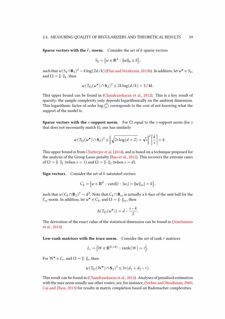
2.4. MEASURING QUALITY OF REGULARIZERS AND THEORETICAL RESULTS 59
Sparse vectors with the ℓ1-norm. Consider the set of k-sparse vectors
Sk =w ∈Rd : ‖w‖0 ≤ k
,
such thatw(Sk∩B2)2 ∼ k log(2d/k) (Plan and Vershynin, 2013b). In addition, letw⋆ ∈ Sk ,
and Ω = ‖ · ‖1, then
w(TΩ(w⋆)∩S2)2 ≤ 2k log(d/k) + 5/4k.
This upper bound can be found in (Chandrasekaran et al., 2012). This is a key result of
sparsity: the sample complexity only depends logarithmically on the ambient dimension.
This logarithmic factor of order log (dk) corresponds to the cost of not knowing what the
support of the model is.
Sparse vectors with the s-support norm. For Ω equal to the s-support norm (for sthat does not necessarily match k), one has similarly
w(TΩ(w⋆)∩S2)2 ≤
[√2s log(d + 2) +
√s]2 ⌈k
s
⌉+ k.
This upper bound is from Chatterjee et al. (2014), and is based on a technique proposed for
the analysis of the Group Lasso penalty (Rao et al., 2012). This recovers the extreme cases
of Ω = ‖ · ‖1 (when s = 1) and Ω = ‖ · ‖2 (when s = d).
Sign vectors. Consider the set of k-saturated vectors
Ck =w ∈Rd : cardi : |wi |= ‖w‖∞= k
,
such that w(Ck∩B2)2 = d2. Note that Ck∩B∞ is actually a k-face of the unit ball for the
ℓ∞-norm. In addition, let w⋆ ∈ Ck , and Ω = ‖ · ‖∞, then
∆(TΩ(w⋆)) = d − s − k
2.
The derivation of the exact value of the statistical dimension can be found in (Amelunxen
et al., 2013).
Low-rank matrices with the trace norm. Consider the set of rank r matrices
Lr =W ∈Rd1×d2 : rank(W ) = r
.
ForW ⋆ ∈ Lr , and Ω = ‖ · ‖∗, then
w(TΩ(W⋆)∩S2)2 ≤ 3r(d1+ d2 − r).
This result can be found in (Chandrasekaran et al., 2012). Analyses of penalized estimation
with themax norm usually use other routes, see, for instance, (Srebro and Shraibman, 2005;
Cai and Zhou, 2013) for results in matrix completion based on Rademacher complexities.

60 CHAPTER 2. PENALIZED MATRIX ESTIMATION
Nonnegative entries. In most of the previous cases, one may additionally incorporate
the knowledge that the model only has nonnegative entries, such that the ambient space
becomes Rd+ (Donoho and Tanner, 2010). In some particular settings (e.g., using non-
Gaussian designs), this has been shown to lead to a surprising sample complexity of order
k for exact recovery of k-sparse nonnegative vectors (Donoho and Tanner, 2005; Wang
and Tang, 2009) using a simple feasibility problem as in Section 2.4.2. This corresponds to
strictlymore than a constant factor improvement over sample complexities of order k logd ,as this is completely dimension-independent. In other settings, however, it is frequent to
observe only constant factor improvements.
2.4.6 Estimation with Non-gaussian Designs
Drawing inspiration from the domain of random projections at large, various conditions
have been proposed (usually in specic cases) to ensure that a non-Gaussian (but possibly
still random) design may lead to exact recovery. This includes the Random Fourier en-
semble, the Bernoulli ensemble or Count-Min matrices (Berinde et al., 2008). Many of the
associated analyses are specic to ℓ1-norm minimization (and ℓ0-sparse models), and rely
on properties such as Restricted Isometry Property (Berinde et al., 2008), or the Null Space
Property (Cohen et al., 2009). Testing whether these properties hold on xed matrices is
usually NP-hard, although relaxations have been proposed (d’Aspremont and El Ghaoui,
2011). Recently, an imposed real world design has been shown to exhibit a phase transition
(Vattikuti et al., 2014), but such examples remain scarce.
The use of nonlinear models and designs is of course an interesting area (Plan and Ver-
shynin, 2013b). An interesting such example consists in using quantized measurements.
Indeed, in all the previous designs, measurements are assumed to be a vector in RN , where
components are encoded with innite precision. In practice, this is rarely the case as most
measurement systems have a limited dynamic and can handle a limited number of bits per
measurement. In addition to this, the oating point arithmetic used in the computers has
also a limited bit resolution. Hence, the bit resolution is potentially limited at many stages.
Consider a quantization operator Q : R→ 1, . . . ,K over an alphabet (c1, . . . ,cK ) ∈ RK
of length K . A quantized linear model can be obtained as
yi = Q(〈ai ,w〉), i ∈ [N ].
In the extreme case, the alphabet can reduce to (−1,1) only: that is, only the sign of the
projection is measured:
yi = sign(〈ai ,w〉), i ∈ [N ].
This model is referred to as one-bit compressed sensing. This also corresponds to random
hyperplane hashing, which is a hashing scheme for approximating the angular similarity
θ(w1,w2) = 1− 1
πcos−1
( 〈w1,w2〉‖w1‖2‖w2‖2
)
between vectorsw1,w2 ∈Rd . Consider the Hamming distance dH(x,y) =∑Ni=1 xiyi over
the boolean hypercube 0,1N . An estimation of the angle between any two pair of vectors
can be obtained through the Hamming distance between the one-bit observations in the
corresponding models: with N observations, and A a random Gaussian design,
E
[1
NdH(sign(Aw1), sign(Aw2))
]=θ(w1,w2)
π.

2.4. MEASURING QUALITY OF REGULARIZERS AND THEORETICAL RESULTS 61
a1
a2
a3
a4
a5a6
a7
a8
a9
w⋆
Figure 2.11: Illustration of random hyperplane hashing
This is natural, as illustrated in Figure 2.11, as the Hamming distance counts the number of
circular sectors where both vectors get projected, and averaging over many hyperplanes
provides an estimation of the angle. A similar intuition carries over to the estimation
problem, and recently, many works have considered the question of characterizing when
exact or robust recovery is possible with this type of measurements (Gupta et al., 2010).
As shown by Plan and Vershynin (2013a), in the one-bit setting, robust recovery up to
precision ε can be achieved with about the same number of measurements based on the
squared Gaussian width, albeit with a worse dependence on ε.


3Estimation of Sparse and Low Rank
MatricesContents
3.1 Introduction . . . . . . . . . . . . . . . . . . . . . . . . . . . . . . . . . . . 64
3.1.1 Model . . . . . . . . . . . . . . . . . . . . . . . . . . . . . . . . . . 65
3.1.2 Main Examples . . . . . . . . . . . . . . . . . . . . . . . . . . . . . 65
3.1.3 Outline . . . . . . . . . . . . . . . . . . . . . . . . . . . . . . . . . . 65
3.1.4 Notation . . . . . . . . . . . . . . . . . . . . . . . . . . . . . . . . . 66
3.2 Oracle Inequality . . . . . . . . . . . . . . . . . . . . . . . . . . . . . . . . 66
3.3 Generalization Error in Link Prediction . . . . . . . . . . . . . . . . . . . . 67
3.4 Algorithms . . . . . . . . . . . . . . . . . . . . . . . . . . . . . . . . . . . . 68
3.4.1 Proximal Operators . . . . . . . . . . . . . . . . . . . . . . . . . . . 68
3.4.2 Generalized Forward-backward Splitting . . . . . . . . . . . . . . . 69
3.4.3 Incremental Proximal Descent . . . . . . . . . . . . . . . . . . . . . 69
3.4.4 Positive Semi-denite Constraint . . . . . . . . . . . . . . . . . . . 70
3.5 Recovering Clusters . . . . . . . . . . . . . . . . . . . . . . . . . . . . . . . 70
3.6 Numerical Experiments . . . . . . . . . . . . . . . . . . . . . . . . . . . . . 71
3.6.1 Synthetic Data . . . . . . . . . . . . . . . . . . . . . . . . . . . . . 71
3.6.2 Real Data Sets . . . . . . . . . . . . . . . . . . . . . . . . . . . . . . 71
3.7 Discussion . . . . . . . . . . . . . . . . . . . . . . . . . . . . . . . . . . . . 73
3.7.1 Other Loss Functions . . . . . . . . . . . . . . . . . . . . . . . . . . 73
3.7.2 Optimization . . . . . . . . . . . . . . . . . . . . . . . . . . . . . . 74
3.7.3 Geometry . . . . . . . . . . . . . . . . . . . . . . . . . . . . . . . . 74
3.7.4 Factorization Methods . . . . . . . . . . . . . . . . . . . . . . . . . 75
3.8 Proofs . . . . . . . . . . . . . . . . . . . . . . . . . . . . . . . . . . . . . . . 78
3.8.1 Sketch of Proof of Proposition 13 . . . . . . . . . . . . . . . . . . . 78
3.8.2 Proof of Proposition 16 . . . . . . . . . . . . . . . . . . . . . . . . . 79

64 CHAPTER 3. ESTIMATION OF SPARSE AND LOW RANK MATRICES
3.1 Introduction
Matrix estimation is at the center of many modern applications and theoretical advances
in the eld of high dimensional statistics. The key element which dierentiates this prob-
lem from standard high dimensional vector estimation lies in the structural assumptions
that can be formulated in this context. Indeed, the notion of sparsity assumption has been
transposed into the concept of low rank matrices and opened up the way to numerous
achievements (Srebro, 2004; Cai et al., 2008). In this chapter, we argue that being low rank
is not only an equivalent of sparsity for matrices but that being low rank and sparse can
actually be seen as two orthogonal concepts. The underlying structure we have in mind is
that of a block diagonal matrix. This situation occurs for instance in covariance matrix es-
timation in the case of groups of highly correlated variables or when denoising/clustering
social graphs.
Ecient procedures developed in the context of sparse model estimation mostly rely
on the use of ℓ1-norm regularization (Tibshirani, 1996a). Natural extensions include cases
where subsets of related variables are known to be active simultaneously (Yuan and Lin,
2006). These methods are readily adapted to matrix valued data and have been applied
to covariance estimation (El Karoui, 2009; Bien and Tibshirani, 2010) and graphical model
structure learning (Banerjee et al., 2008; Friedman et al., 2008). In the low rank matrix
completion problem, the standard relaxation approach leads to the use of the trace norm
as themain regularizer within the optimization procedures (Srebro et al., 2005; Koltchinskii
et al., 2011a) and their resolution can either be obtained in closed form (loss measured in
terms of Frobenius norm) or through iterative proximal solutions (Combettes and Pesquet,
2011; Beck and Teboulle, 2009) (for general classes of losses). However, solutions of low
rank estimation problems are in general not sparse at all, while denoising and variable
selection on matrix-valued data are blind to the global structure of the matrix and process
each variable independently. In this chapter, we study the benets of using the sum of
ℓ1 and trace-norms as regularizer. This sum of regularizers on the same object allows to
benet from the virtues of both of them, in the sameway as the elastic-net (Zou andHastie,
2005a) combines the sparsity-inducing property of the ℓ1 normwith the smoothness of the
quadratic regularizer.
The trace norm and the ℓ1 regularizers have already been combined in a dierent con-
text. In Robust PCA (Candès et al., 2011) and related literature, the signal W is assumed
to have an additive decompositionW = X + Y where X is sparse and Y low rank. Note
that W is not in general sparse nor low rank and that this decomposition is subject to
identiability issues, as analyzed, e.g., in (Chandrasekaran et al., 2011). The decomposi-
tion is recovered by using ℓ1-norm regularization over X and trace norm regularization
over Y . This technique has been successfully applied to background substraction in image
sequences, to graph clustering (Jalali et al., 2011) and covariance estimation (Luo, 2011).
We would like to emphasize that this type of demixing problems are largely dierent from
what we consider here.
Here, we consider the dierent situation where a single matrixW is both sparse and
low rank at the same time. We demonstrate the applicability of ourmixed penalty on dier-
ent problems. We develop proximal methods to solve these convex optimization problems
and we provide numerical evidence as well as theoretical arguments which illustrate the
trade-o which can be achieved with the suggested method.

3.1. INTRODUCTION 65
3.1.1 Model
For amatrixW = (Wi,j)i,j , wewill consider the followingmatrix norms: ‖W ‖1 =∑i,j |Wi,j |
and ‖W ‖∗ =∑rank(W )i=1 σi(W ). We consider the following setup. Let Y ∈ Rd×d be an ob-
served matrix and ℓ : Rd×d ×Rd×d →R+ a loss function over matrices. We introduce the
following optimization problem:
argminW∈W
[ℓ(W ,Y ) + γ‖W ‖1+ τ‖W ‖∗]
for some convex admissible setW ⊂ Rd×d and nonnegative regularization parameters γand τ.
3.1.2 Main Examples
The underlying assumption in this work is that the unknown matrix to be recovered has
a block-diagonal structure. We now describe the main modeling choices through the fol-
lowing motivating examples:
• Example 5: Covariance matrix estimation - the matrix Y represents a noisy estimate
of the true covariance matrix obtained for instance with very few observations; the
search space isW = S+ the class of positive semi-denite matrices; for the loss, we
consider the squared norm ℓ(W ,Y ) = ‖W −Y‖2F .
• Graph denoising - the matrix Y is the adjacency matrix of a noisy graph with both ir-
relevant and missing edges; the search space is all ofW = Rd×d and the coecients
of a candidatematrix estimate S are interpreted as signed scores for adding/removing
edges from the original matrix Y ; again, we use ℓ(W ,Y ) = ‖W −Y‖2F .
• Example 6: Link prediction - the matrix Y is the adjacency matrix of a partially
observed graph: entries are 0 for both not-existing and undiscovered links. The
search space is unrestricted as before and the matrixW contains the scores for link
prediction; the ideal loss function is the empirical average of the zero-one loss for
each coecient
ℓE(W ,Y ) =1
|E|∑
(i,j)∈E1(Yi,j − 1/2) ·Wi,j ≤ 0,
where E is the set of edges in Y . However, as in classication theory, practical
algorithms should use a convex surrogate (e.g., the hinge loss).
3.1.3 Outline
The remainder of this chapter is organized as follows. Sections 3.2 and 3.3 are devoted
to theoretical results on the interplay between sparse and low rank eects. Section 3.4
presents algorithms used for resolution of the optimization problem. Section 3.5 discusses
how clusters can be recovered from matrix estimates and Section 3.6 is devoted to numer-
ical experiments. We close this chapter by giving some perspectives in Sections 3.7. This
chapter is an extended version of a paper with Emile Richard and Nicolas Vayatis which
has appeared in the proceedings of ICML (Richard et al., 2012).

66 CHAPTER 3. ESTIMATION OF SPARSE AND LOW RANK MATRICES
3.1.4 Notation
In the sequel, the projection of a matrix M onto a convex setW is denoted by ΠW (M).The matrix M+ is the componentwise positive part of the matrix M, and sgn(M) is thesign matrix associated to M with the convention sgn(0) = 0. The componentwise or
Hadamard product of matrices is denoted by . The class S+ of matrices is the convex cone
of positive semi-denite matrices inRd×d . The sparsity index ofM is ‖M‖0 = cardMi,j ,
0 and the Frobenius norm of a matrix M is dened by ‖M‖2F =∑i,jM
2i,j . The operator
norm ofM is ‖M‖op = supx : ‖x‖2=1 ‖Mx‖2, while ‖M‖∞ =max |Mi,j |
3.2 Oracle Inequality
The next result shows how matrix recovery is governed by the trade-o between the rank
and the sparsity index of the unknown target matrix, or by their convex surrogates: the
trace norm and the ℓ1-norm.
Proposition 13. LetW ⋆ ∈Rd×d and Y =W ⋆+ǫ with ǫ ∈Rd×d having i.i.d. entries withzero mean. Assume for some α ∈ [0,1] that τ ≥ 2α‖ǫ‖op and γ ≥ 2(1−α)‖ǫ‖∞. Let
W = argminW∈W
[‖W −Y‖2F + γ‖W ‖1+ τ‖W ‖∗
].
Then,
‖W −W ⋆‖2F ≤ infW∈W
[‖W −W ⋆‖2F + 2γ‖W ‖1+ 2τ‖W ‖∗
],
‖W −W ⋆‖2F ≤[2γ‖W ⋆‖1+ 2τ‖W ⋆‖∗
]∧
[γ√‖W ⋆‖0+ τ
√rank(W ⋆)
√2+ 1
2
]2.
The techniques used in the proof, that we defer to Section 3.8.1, are similar to those in-
troduced in (Koltchinskii et al., 2011a). Note that the upper bound interpolates between
the results known for trace-norm penalization and Lasso. In fact, for α = 0, τ can be set
to zero, and we get a sharp bound for Lasso, while the trace-norm regression bounds of
(Koltchinskii et al., 2011a) are obtained for α = 1.
From a theoretical point of view, Proposition 13 provides us with performance guar-
antees when the regularization parameters are large enough. From random matrix theory,
the operator norm of a randomGaussianmatrix is known to concentrate around√d , which
enforces a stringent constraint on τ for τ ≥ 2α‖ǫ‖op to hold with high probability. Sim-
ilarly, the ∞-norm ‖ǫ‖∞ can be bounded by ‖ǫ‖op or using the multivariate Tchebyche
inequality of Olkin and Pratt (1958) which implies that the condition γ ≥ 2(1 − α)‖ǫ‖∞is satised with probability 1 − δ when γ = Ω
((1−α)2dσδ
). In practice, γ should not
exceed the order of magnitude of the entries of the matrix, as this leads to a trivial zero
solution. Asymptotically, to keep the sparsity regularization parameter γ of the order of
magnitude of elements of the observation matrix Y , the free parameter α must be chosen
so that 1 − αd ∼d 1d . This gives the same asymptotic behavior in O(
√d) for the lower
bound on τ as in matrix completion.
The proof can also easily be extended to more general xed matrix designs where
observations are of the form yi = 〈Xi ,W ⋆〉+ εi for i ∈ [N ]. In this case, the bound is in

3.3. GENERALIZATION ERROR IN LINK PREDICTION 67
terms of the design-dependant norm given by
‖W −W ⋆‖=
√√√N∑
i=1
〈Xi ,W −W ⋆〉2.
Proposition 13 corresponds to a design X1, . . . ,Xd2 which is the canonical basis of Rd×d .
3.3 Generalization Error in Link Prediction
We dwell for a moment on the task of link prediction in order to illustrate how rank and
sparsity constraints can help in this setting. Consider a graph over d vertices with adja-
cency matrix Y ∈ 0,1d×d , and a subset E of coordinates (i, j) ∈ [d] × [d] of this matrix
that have been observed: for (i, j) ∈ E, the value Yi,j ∈ 0,1 is known to the experimenter.
We set out to predict the values of the remaining entries of Y by nding a sparse rank rpredictorW ∈Rd×d with small zero-one loss
ℓ(W ,Y ) =1
d2
∑
(i,j)∈[d]×[d]1(Yi,j − 1/2) ·Wi,j ≤ 0
by minimizing the empirical zero-one loss
ℓE(W ,Y ) =1
|E|∑
(i,j)∈E1(Yi,j − 1/2) ·Wi,j ≤ 0.
The objective of a generalization bound is to relate ℓ(W ,Y ) with ℓE(W ,Y ). In the case
of the sole rank constraint, Srebro (2004) remarked that all low rank matrices with the
same sign pattern are equivalent in terms of loss and applied a standard argument for
generalization in classes of nite cardinality. In the work of Srebro, a beautiful argument
is used to upper bound the number of distinct sign congurations for predictors of rank r
slr(d,r) = cardsgn(W ) |W ∈Rd×d ,rank(W ) ≤ r|
leading to the following generalization performance: for δ > 0, Y ∈ 0,1d×d and with
probability 1 − δ over choosing a subset E of entries in 1, . . . ,d2 uniformly among all
subsets of |E| entries, we have for any matrixW of rank at most r and ∆(d,r) =(8edr
)2dr
that
ℓ(W ,Y ) < ℓE(W ,Y ) +
√log∆(d,r)− logδ
2|E| . (3.1)
We consider the class of sparse rank r predictors
M(d,r,s) = UV T |U ,V ∈ Rd×r , ||U ||0+ ||V ||0 ≤ s
and let ssplr(d,r,s) be the number of sign congurations for the setM(d,r,s). By upper
bounding the number of sign congurations for a xed sparsity pattern in (U ,V ) usingan argument similar to (Srebro, 2004), a union bound gives
ssplr(d,r,s) ≤ Γ(d,r,s) =
(16ed2
s
)s (2dr
s
).

68 CHAPTER 3. ESTIMATION OF SPARSE AND LOW RANK MATRICES
Using the same notations as previously, we deduce from this result the following general-
ization bound: with probability 1− δ and for allW ∈M(d,r,s),
ℓ(W ,Y ) < ℓE(W ,Y ) +
√logΓ(d,r,s)− logδ
2|E| . (3.2)
In general, the square-root deviation term in bound (3.2) is smaller than the one in (3.1) for
suciently large values of d as shown in the next proposition. The two bounds coincide
when s = 2dr , that is, when (U ,V ) is dense and there is no sparsity constraint.
Proposition 14. For rd = dβ with β ∈]0,1] and sd = dα with α ≤ 2β,
∆(d,rd)
Γ(d,rd ,sd)=Ω
[8ed(βd −α)
(βd)2
]2d2β ,
which diverges when d goes to innity.
Proof. The result follows from the application of Stirling’s formula.
By considering a predictor class of lower complexity than low rank matrices, we can thus
achieve better generalization performances. Although this illustrates that combining rank
and sparsity allows to improve generalization performance, minimizing the classication
error overM(d,r,s) does not lead to a practical procedure.
3.4 Algorithms
We now present how to solve the optimization problem with the proposed regularizer.
We consider a loss function ℓ(W ,Y ) convex and dierentiable inW , and assume that its
gradient is Lipschitz with constant L and can be eciently computed. This is, in particular,
the case for the previously mentioned squared Frobenius norm, and for other classical
choices such as the logistic loss.
3.4.1 Proximal Operators
We encode the presence of a constraint setW using the indicator function δW (W ) that iszero whenW ∈W and∞ otherwise, leading to
W = argminW∈Rd×d
[ℓ(W ,Y ) + τ‖W ‖1+ γ‖W ‖∗+ δW (W )] .
This formulation involves a sumof a convex dierentiable loss and of convex non-dierentiable
regularizers which renders the problem non trivial. A string of algorithms have been de-
veloped for the case where the optimal solution is easy to compute when each regularizer
is considered in isolation. Formally, this corresponds to cases where the proximal operator
dened for a convex regularizer Ω : Rd×d →R at a point Z by
proxΩ
(Z) = argminW∈Rd×d
[1
2‖W −Z‖2F +Ω(W )
]

3.4. ALGORITHMS 69
is easy to compute for each regularizer taken separately. See (Combettes and Pesquet,
2011; Parikh and Boyd, 2013) for a broad overview of proximal methods.
The proximal operator of the indicator function is simply the projection ontoW , which
justies the alternate denomination of generalized projection operator for proxΩ . The
proximal operator for the trace norm is given by the shrinkage operation as follows (Beck
and Teboulle, 2009). If Z = U diag(σ1, · · · ,σd)V T is the singular value decomposition of
Z ,SHRτ(Z) = prox
τ‖·‖∗(Z) = U diag((σi − τ)+)iV T .
Similarly, the proximal operator for the ℓ1-norm is the soft thresholding operator
STγ (Z) = proxγ‖·‖1
= sgn(Z) (|Z | −γ)+.
3.4.2 Generalized Forward-backward Splitting
The family of Forward-Backward splitting methods are iterative algorithms applicable
when there is only one non-dierentiable regularizer. These methods alternate a gradi-
ent step and a proximal step, leading to updates of the form
Wk+1 = proxθΩ
(Wk −θ gradW ℓ(Wk ,Y )),
for a stepsize θ. In particular, this corresponds to projected gradient descent when Ω
is the indicator function of a convex set. On the other hand, Douglas-Rachford splitting
tackles the case of q ≥ 2 terms but does not benet from dierentiability. A generalization
of these two setups has been recently proposed in (Raguet et al., 2013) under the name of
Generalized Forward-Backward, which we specialize to our problem in Algorithm 1. The
proximal operators are applied in parallel, and the resulting (Z1,Z2,Z3) is projected ontothe constraint that Z1 = Z2 = Z3 which is given by the mean. The auxiliary variable
Z3 can be simply dropped when W = Rd×d . The algorithm converges under very mild
conditions when the step size θ is smaller than 2L .
Algorithm 1 Generalized Forward-Backward
InitializeW ,Z1,Z2,Z3 = Y , q = 3
repeat
Compute G = ∇W ℓ(W ,Y ).Compute Z1 = proxqθτ‖·‖∗(2W −Z1 −θG)Compute Z2 = proxqθγ‖·‖1(2W −Z2 −θG)Compute Z3 =ΠW (2W −Z3 −θG)SetW = 1
q
∑qk=1Zk
until convergence
return W
3.4.3 Incremental Proximal Descent
Although Algorithm 1 performs well in practice, theO(d2)memory footprint with a large
leading constant due to the parallel updates can be a drawback in some cases. As a conse-
quence, we mention a matching serial algorithm (Algorithm 2) introduced in (Bertsekas,

70 CHAPTER 3. ESTIMATION OF SPARSE AND LOW RANK MATRICES
2011) that has a avor similar to multi-pass stochastic gradient descent. We present here
a version where updates are performed according to a cyclic order, although random se-
lection of the order of the updates is also possible.
Algorithm 2 Incremental Proximal Descent
InitializeW = Yrepeat
SetW =W −θ∇W ℓ(W ,Y )SetW = proxθτ‖·‖∗(W )SetW = proxθγ‖·‖1(W )
SetW =ΠW (W )until convergence
return W
3.4.4 Positive Semi-denite Constraint
For any positive semi-denite matrix, we have ‖Z‖∗ = Tr(Z). The simple form of the trace
norm allows to take into account the positive semi-denite constraint at no additional
cost, as the shrinkage operation and the projection onto the convex cone of positive semi-
denite matrices can be combined into a single operation.
Lemma 1. For τ ≥ 0 andW ∈Rd×d ,
proxτ‖·‖∗+δS+
(W ) = argminZ0
[1
2‖Z −W ‖2F + τ‖Z‖∗
]=ΠS+ (W − τI) .
3.5 Recovering Clusters
The estimators described previously may allow to estimate a covariance or adjacency ma-
trix, but not to directly recover clusters or groups. Although outside of the scope of this
work, we mention here a few methods which could be used.
Consider a symmetric and sparse square matrixW ∈Rd×d . This can be viewed as the
adjacency matrix of a graph G = (V ,E), where V = [d], and E = (i, j) : Wi,j > 0. Thegraph bandwidth allow to measure to what extent a graph corresponds to a chain of some
order.
Denition 9 (Graph Bandwidth). The graph bandwidth of matrixW (or graph G) is
GBW(W ) =minf ∈Sd
max|f (i)− f (j)| : Wi,j > 0
,
where Sd is the set of all permutations f : [d]→ [d].
For instance,
GBW
1 1. . .
1 1
= GBW
1 1
1 1. . .
1
= 2.

3.6. NUMERICAL EXPERIMENTS 71
The path graph on d vertices has bandwidth 1, while a star over k+ 1 vertices has band-
width ⌊(k − 1)/2⌋+ 1. The Cuthil-McKee algorithm (Cuthill and McKee, 1969) seeks to
simultaneously permute the lines and rows ofW such that the resulting matrix is banded
with the smallest bandwidth. This is done in a Breadth-First Search (BFS) manner: x
a vertex, and visit each of its neighbor in the reverse order of their degrees. This is an
heuristic, as both the optimal ordering and the associated cost are NP-hard to nd, but
that can still be used to reorder estimators. More elaborate methods have been proposed
to estimate the bandwidth (Blum et al., 1998; Dunagan and Vempala, 2001), although these
cannot usually be used on large scale data. Alternate notions of bandwidths have been
proposed, such as the 2-SUM, where the squared dierence is used in place of the abso-
lute dierence. In this case as well, various relaxations have been proposed by Fogel et al.
(2013).
Although this may allow for easier visual inspection and representation, this still does
not output clusters. The literature on clustering weighted or unweighted graphs (also
often referred to as community detection, by analogy with social networks) is ample, and
we refer the reader on this topic to surveys by Fortunato (2010) and Von Luxburg (2007),
and to Section 3.7 on factorization-based methods.
3.6 Numerical Experiments
We present numerical experiments to highlight the benets of our method. For eciency
reasons, we use the serial proximal descent algorithm (Algorithm 2).
3.6.1 Synthetic Data
Covariance matrix estimation. We draw N vectors xi ∼ N (0,Σ) for a block diagonal co-
variance matrix Σ ∈Rn×n. We use r blocks of random sizes and of the form vv⊤ where theentries of v are drawn i.i.d. from the uniform distribution on [−1,1]. Finally, we add Gaus-sian noiseN (0,σ2) on each entry. In our experiments r = 5,N = 20, d = 100, σ = 0.6.
We apply our method (SPLR), as well as trace norm regularization (LR) and ℓ1 norm regu-
larization (SP) to the empirical covariance matrix, and report average results over ten runs.
Figure 3.1 shows the RMSE normalized by the norm of Σ for dierent values of τ and γ .Note that the eect of the mixed penalty is visible as the minimum RMSE is reached in-
side the (τ,γ) region. We perform, on the same data, separate cross-validations on (τ,γ)for SPLR, on τ for LR and on γ for SP. We show in Figure 3.2 the supports recovered by
each algorithm, the output matrix of LR being thresholded in absolute value. The support
recovery demonstrates how our approach discovers the underlying patterns despite the
noise and the small number of observations.
3.6.2 Real Data Sets
Protein Interactions. We use data from Hu et al. (2009), in which protein interactions in
Escherichia coli bacteria are scored by strength in [0,2]. The data is, by nature, sparse. In
addition to this, it is often suggested that interactions between two proteins are governed
by a small set of factors, such as surface accessible amino acid side chains Bock and Gough
(2001), which motivates the estimation of a low rank representation. Representing the
data as a weighted graph, we lter to retain only the 10% of all 4394 proteins that exhibit

72 CHAPTER 3. ESTIMATION OF SPARSE AND LOW RANK MATRICES
Figure 3.1: Covariance estimation. Cross-validation: normalized RMSE scores (SPLR)
True cov. n =20 ,N =100 ,σ = 0.6 Sparse RMSE=0.6
Low−Rank RMSE=0.685 SP&LR RMSE=0.549
Figure 3.2: Covariance estimation. Support of Σ (top left), and of the estimates given by
SP (top right), LR (bottom left), and SPLR (bottom right)
the most interactions as measured by weighted degree. We corrupt 10% of entries of the
adjacency matrix selected uniformly at random by uniform noise in [0,η]. Parameters
are selected by cross-validation and algorithms are evaluated using mean RMSE between
estimated and original adjacency matrices over 25 runs. RMSE scores are shown in Table
3.1 and show the empirical superiority of our approach (SPLR).
η SPLR LR SP
0.1 0.0854 ±0.012 0.1487 ±0.02 0.1023 ±0.020.2 0.2073 ± 0.03 0.2673 ± 0.3 0.2484 ± 0.030.3 0.3105 ± 0.03 0.3728 ± 0.03 0.3104 ± 0.02
Table 3.1: Prediction of interactions in Escherichia coli. Mean normalized RMSE and stan-
dard deviations.
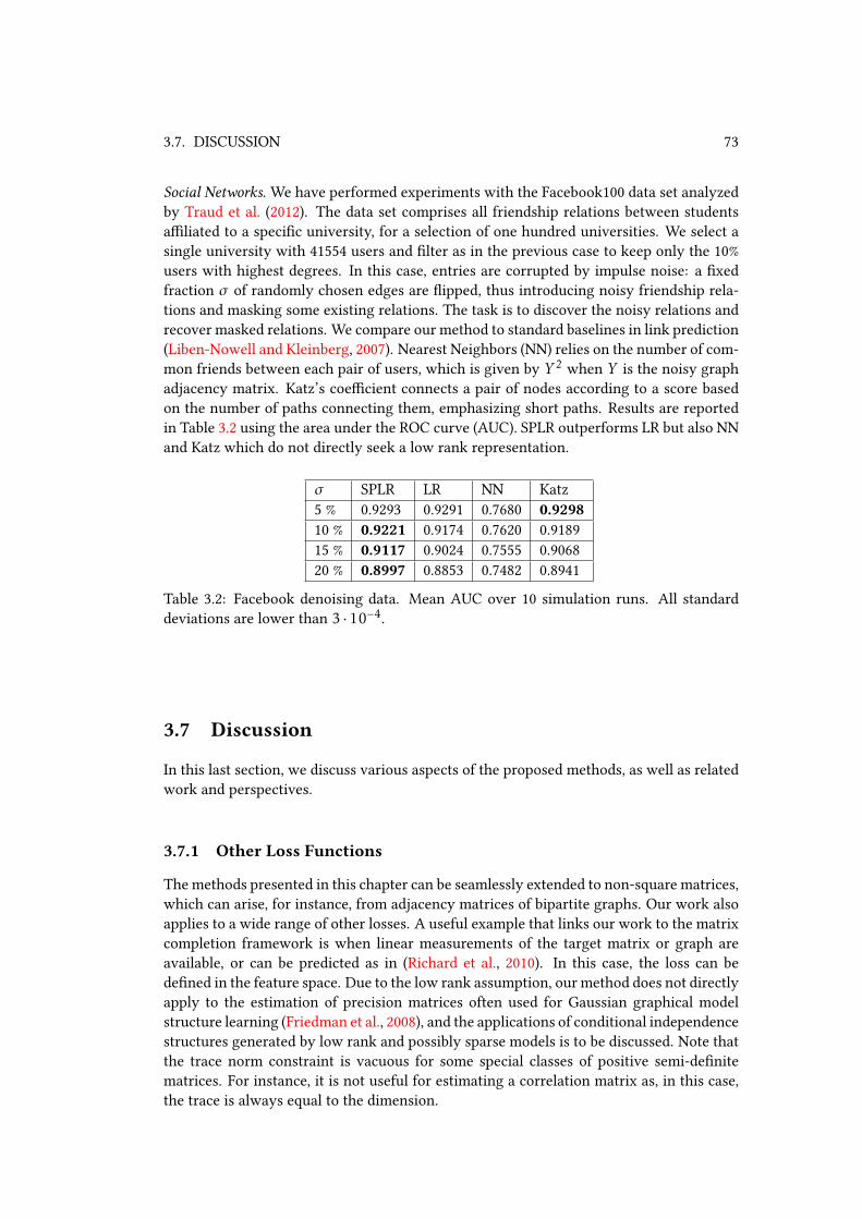
3.7. DISCUSSION 73
Social Networks. We have performed experiments with the Facebook100 data set analyzed
by Traud et al. (2012). The data set comprises all friendship relations between students
aliated to a specic university, for a selection of one hundred universities. We select a
single university with 41554 users and lter as in the previous case to keep only the 10%
users with highest degrees. In this case, entries are corrupted by impulse noise: a xed
fraction σ of randomly chosen edges are ipped, thus introducing noisy friendship rela-
tions and masking some existing relations. The task is to discover the noisy relations and
recover masked relations. We compare our method to standard baselines in link prediction
(Liben-Nowell and Kleinberg, 2007). Nearest Neighbors (NN) relies on the number of com-
mon friends between each pair of users, which is given by Y 2 when Y is the noisy graph
adjacency matrix. Katz’s coecient connects a pair of nodes according to a score based
on the number of paths connecting them, emphasizing short paths. Results are reported
in Table 3.2 using the area under the ROC curve (AUC). SPLR outperforms LR but also NN
and Katz which do not directly seek a low rank representation.
σ SPLR LR NN Katz
5 % 0.9293 0.9291 0.7680 0.9298
10 % 0.9221 0.9174 0.7620 0.9189
15 % 0.9117 0.9024 0.7555 0.9068
20 % 0.8997 0.8853 0.7482 0.8941
Table 3.2: Facebook denoising data. Mean AUC over 10 simulation runs. All standard
deviations are lower than 3 · 10−4.
3.7 Discussion
In this last section, we discuss various aspects of the proposed methods, as well as related
work and perspectives.
3.7.1 Other Loss Functions
The methods presented in this chapter can be seamlessly extended to non-square matrices,
which can arise, for instance, from adjacency matrices of bipartite graphs. Our work also
applies to a wide range of other losses. A useful example that links our work to the matrix
completion framework is when linear measurements of the target matrix or graph are
available, or can be predicted as in (Richard et al., 2010). In this case, the loss can be
dened in the feature space. Due to the low rank assumption, our method does not directly
apply to the estimation of precision matrices often used for Gaussian graphical model
structure learning (Friedman et al., 2008), and the applications of conditional independence
structures generated by low rank and possibly sparse models is to be discussed. Note that
the trace norm constraint is vacuous for some special classes of positive semi-denite
matrices. For instance, it is not useful for estimating a correlation matrix as, in this case,
the trace is always equal to the dimension.

74 CHAPTER 3. ESTIMATION OF SPARSE AND LOW RANK MATRICES
3.7.2 Optimization
Other optimization techniques can be considered for future work. A trace norm constraint
alone can be taken into account without projection or relaxation into a penalized form by
casting the problem as a semi-denite program as proposed by Jaggi (2013). The special
form of this semi-denite program can be leveraged to use the ecient resolution tech-
nique from (Hazan, 2008)., based on the Frank-Wolfe algorithm. This method applies to
a dierentiable objective whose curvature determines the performances. Extending these
methods with projection onto the ℓ1 ball or a sparsity-inducing penalty could lead to in-
teresting developments.
3.7.3 Geometry
A major drawback of the proposed method is that the unit ball of the proposed penalty
has extreme points that are either sparse or low rank, but that are not usually both. In
a recent analysis (Drusvyatskiy et al., 2014) focused on the geometry of the unit ball of
the combined penalty, a more precise characterization of the extremal points is given: any
extremal pointW has to satisfy
r(r + 1)
2≤ k+ 1,
where r and k are the rank and the ℓ0-norm of W , respectively. In addition, they show
that the unit ball of the combined penalty does not have more vertices than the ℓ1-normunit ball. This is not surprising: as we have mentioned in Section 2.4.3, the unit ball for
the trace norm has no vertices, although it has higher-order non-smooth points. However,
it is not clear how relevant the number of vertices (i.e., of maximally non smooth points)
is for recovery. A further analysis of higher-order points of the unit ball of the combined
norm could be fruitful.
We have provided an analysis for recovery of fully-observed but noisy matrices. An
interesting alternate problem consists in characterizing the sample complexity, both with
or without noise, as shown in Chapter 2. As was shown recently based on Gaussian width
arguments (Oymak et al., 2012), the sample complexity is not reduced when combining ℓ1-norm and trace norm for exact or robust recovery with Gaussian designs. This suggests
that the experimental design matters signicantly when designing regularizers.
Another interesting question consists in determining tighter convex relaxations to the
rank and the sparsity. In particular, one may ask what is the convex hull of
W ∈Rd1×d2 : rank(W ) ≤ r, ‖W ‖0 ≤ k
intersected with the ℓ∞-norm ball, or over other balls. However, it may also be that there
are somemore interesting joint measures of rank and sparsity to relax than the intersection
of these two classical manifolds. The ranksity index (Richard et al., 2013) provides such
an alternative measure, along with a convex relaxation based on the trace norm. This
convex penalty has the benet of being non-dierentiable at points which are both low
rank and sparse. Although such a modeling work can also be done through atomic norms
in principle (e.g., considering rank one atoms with limited sparsity), it remains unclear
how the resulting norms can be used in practice.

3.7. DISCUSSION 75
3.7.4 Factorization Methods
A related task is nding low rank factorizations of matrices of the form UV T (Srebro,
2004; Srebro et al., 2005), thus jointly optimizing in U ,V ∈ Rd×r loss functions of theform ℓ((U ,V ),Y ) = ‖UV T −Y‖2F for some target maximum rank r . This implicitly en-
codes the low rank constraint which leads to ecient optimization schemes, and allows
for interpretability as estimated (U ,V ) pairs can be considered as latent factors. Althoughoptimization with the trace norm or the max norm implicitly assumes such a factorization,
factorization-based method work with the factorization directly. Although formulations
are usually convex in U or V, they are not in general jointly convex and optimization pro-
cedures can get stuck in local minima. However, these methods have been associated with
good empirical performances (Xu et al., 2003; Koren, 2008). Factorization methods param-
eterized inU and V are not very practical to control the sparsity ofW = UV T . However,
one may alternatively seek to control the sparsity of the factors U and V , which can lead
to sensible models. In the following, we give more background on these methods, which
could potentially be of interest to dene regularizers based on factorizations.
Sparse Factors
Nonnegative Matrix Factorization (NMF) (Lee et al., 1999) imposes nonnegativity con-
straints on the coecients of U and V to enhance interpretability by allowing only for
additive eects and tends to produce sparse factor matrices U ,V , although this a rather
indirect eect. There is no strong guarantee on the sparsity achieved by NMF nor is it easy
to set the target sparsity. Dierent methods for sparse NMF have been proposed (Hoyer,
2004a; Kim and Park, 2008), where sparsity inducing regularizers are applied on the coef-
cients of the factors. Sparse matrix factorizations have also been proposed without the
positivity constraint, such as for sparse coding (Hoyer, 2002), or for extending the classi-
cal PCA and nding sparse directions that maximize the variance of the projection. This
last problem is often referred to as sparse principal component analysis. SPCA (Zou et al.,
2004) penalizes the ℓ1 norm of the principal components and can be reduced to solving
independent elastic-nets. A dierent formulation using SDP programming is introduced
by d’Aspremont et al. (2007) with good empirical results. In addition, some methods give
up up orthogonality between the components (Mackey, 2009).
An important special case of matrix factorizations is that of rank one factorizations.
The detection of cliqueswithin adjacencymatrices correspond to factorizations of the form
1S1TS where S ⊂ [d] is a set of coordinates. A penalty similar to the one we proposed
has been used in (Ames and Vavasis, 2011) to detect cliques, although with a dierent
loss, which can be shown to lead to exact recovery of the support of the clique in some
circumstances. These types of models are discussed more in the second part of this thesis,
in Chapter 5.
Interpolation of Nuclear Norms
The combined penalty γ‖.‖1 + (1−γ)‖.‖∗ that we propose interpolates between two nu-
clear norms: the trace norm, and the ℓ1-norm. Indeed, from duality with operator norms,

76 CHAPTER 3. ESTIMATION OF SPARSE AND LOW RANK MATRICES
the ℓ1-norm can be expressed in nuclear form as well:
‖W ‖1 = ‖W ‖1→∞ = inf
∑
i
|σi | : W =∑
i
σibiaTi , ‖bi‖1 = ‖ai‖1 = 1
.
The linear combination that we propose is surely not the only way to interpolate between
the ℓ1-norm and the trace norm, and this suggests the following question: what are in-
teresting alternative interpolation methods? A potential choice consists in using semi-
denite programming relaxations: consider
F(X) = γ‖X‖1+ (1−γ)Tr(X),
such that for any u ∈Rn,
F(uuT ) = γ‖u‖21+ (1−γ)‖u‖22.
This allows to dene the following norms.
Denition 10.
‖X‖uv =1
2min
UV T=X
∑
i≥1
F(uiu
Ti ) + F(viv
Ti )
,
‖X‖SDP =1
2min
[Z1X;XTZ2]0F(Z1) + F(Z2)
.
As usual, the dimensions of U and V are not restricted. Although ‖ · ‖uv interpolates
between the trace norm and the ℓ1-norm when γ ∈ [0,1], this norm cannot usually be
computed. However, both the SDP norm and the sum of ℓ1-norm and trace norm are
lower bounds on ‖ · ‖uv, and are thus convex relaxation which can be used in practice.
As it turns out, ‖ · ‖SDP does not interpolate correctly at γ = 1: although for γ = 0,
‖X‖SDP = ‖X‖uv = ‖X‖∗, there exists matrices W such that ‖W ‖SDP < ‖W ‖uv = ‖W ‖1for γ = 1 (consider, for instance, W = [11;1 − 1] ∈ R2×2, which has ‖W ‖1 = 4, but
‖W ‖SDP < 3 < ‖W ‖1.) As a consequence, this does not provide an acceptable interpolation.However, we believe that investigating other interpolations and relaxations along these
lines could be of interest.
Factorization Constants
Straying away from the idea of interpolation between rank and sparsity, one may seek
to dene a penalty directly, using factorizations. Like the trace norm and the max norm,
many more norms can be dened through factorizations.
Proposition 15. Consider normed vector spaces (Rd2 ,‖ · ‖X), (Z ,‖ · ‖Z) and (Rd1 ,‖ · ‖Y ).Then,
γZ(W ) = inf ‖V ‖X→Z‖U‖Z→Y : W = UV is a norm over Rd1×d2 .
Again, the number of columns of U and V in the factorizations is left unbounded. This
type of norm is referred to as a factorization constant, as it measures how well a linear
operator W can be factorized through some latent space Z . This suggests the followingtype of norm.

3.7. DISCUSSION 77
Proposition 16. Consider forW ∈Rd×d the functionals
q(W ) = minUV T=W
‖U‖1‖V ‖1, cr(W ) = minU∈Rd×rV∈Rd×rUV T=W
‖U‖1‖V ‖1.
Then, q is a norm over Rd×d , but c2 is not a norm over R2×2.
The proof is deferred to Section 3.8.2. Although leaving the number of factors unbounded
yields a normwhich can measure sparsity of factorizations, this norm cannot be computed
in practice. On this other hand, capping the number of factors even at the ambient dimen-
sion does not necessarily leads to a convex function. Again, we believe that variations on
this type of approach could be developed and yield interesting results.

78 CHAPTER 3. ESTIMATION OF SPARSE AND LOW RANK MATRICES
3.8 Proofs
3.8.1 Sketch of Proof of Proposition 13
Proof. For any W inW and by optimality of W ,
−2〈W −W ,W ⋆〉 ≤ 2α‖W −W ‖∗‖ǫ‖op+ 2(1−α)‖W −W ‖1‖ǫ‖∞+ τ(‖W ‖∗ − ‖W ‖∗) + γ(‖W ‖1 − ‖W ‖1) + ‖W ‖2F − ‖W ‖2F
for any α ∈ [0;1]. The assumptions on τ,γ and triangular inequality lead to the rst
bound.
Let r = rank(W ), k = ‖W ‖0,W =∑rj=1σjujv
⊤j the SVD ofW ,W = Θ |W |, where
Θ = sgn(W ), and Θ⊥ ∈ 0,1d×d the complementary sparsity pattern. We use PW⊥1 (resp.
PW⊥2 ) to denote the projection operator onto the orthogonal of the left (resp. right) singularspace ofW . We also note PW (X) = X −PW⊥1 XPW⊥2 such that X = PW (X) + PW⊥1 XW
⊥2.
Any element V of the subgradient of the convex functionW 7→ τ‖W ‖∗+γ‖W ‖1 canbe decomposed as
V = τ
( r∑
j=1
ujv⊤j + PW1⊥Q∗PW2⊥
)+ γ
(Θ+Q1 Θ⊥
)
for Q1,Q∗ with ‖Q∗‖op ≤ 1, ‖Q1‖∞ ≤ 1, which can be chosen such that
⟨V ,W −W
⟩= τ
⟨ r∑
j=1
ujv⊤j ,W −W
⟩+ τ‖PW1⊥WPW2⊥‖∗+ γ〈Θ,W −W 〉+ γ‖Θ⊥ W ‖1 .
By monotonicity of the subdierential and optimality conditions,
2〈W −W ⋆ ,W −W 〉 ≤ 2〈ǫ,W −W 〉 − τ⟨ r∑
j=1
ujv⊤j ,W −W
⟩
− τ‖PW⊥1 WPW⊥2 ‖∗ −γ〈Θ,W −W 〉 −γ‖Θ⊥ W ‖1 .
Decompose
ǫ = α
(PW (ǫ) + PW⊥1 ǫPW
⊥2
)+ (1−α)
(|Θ| ǫ+Θ
⊥ ǫ).
Using results on dual norms, we have
|〈M1,M2〉| ≤ ‖M1‖∗‖M2‖op|〈M1,M2〉| ≤ ‖M1‖1‖M2‖∞
for allM1,M2 ∈Rn×n and hence,
〈ǫ,W −W 〉 ≤ α‖PW (ǫ)‖F‖PW1(W −W )PW2
‖F+α‖PW⊥1 ǫPW⊥2 ‖op‖PW⊥1 SPW⊥2 ‖∗+ (1−α)‖Θ ǫ‖F‖Θ
(W −W
)‖F
+ (1−α)‖Θ⊥ ǫ‖∞‖Θ⊥ W ‖1 .

3.8. PROOFS 79
Using
‖PW (ǫ)‖F ≤√2 r‖ǫ‖op, ‖Θ ǫ‖F ≤
√k‖ǫ‖∞
leads for τ ≥ 2α ‖ǫ‖op and γ ≥ 2(1−α)‖ǫ‖∞ to
‖W −W ⋆‖2F + ‖W − S‖2F≤ ‖W −W ⋆‖2F +
(τ√r(√2+ 1) + 2γ
√k
)‖W −W ‖F .
Using βx − x2 ≤(β2
)2, we obtain
‖W −W ⋆‖2F ≤ ‖W −W ⋆‖2F +1
4
(√rτ(√2+ 1) + 2
√kγ
)2
and settingW =W ⋆ gives the result.
3.8.2 Proof of Proposition 16
Proof. q is a norm from the previous proposition, as the ℓ1-norm is an operator norm. Let
X = uvT ∈Rd×d a rank one matrix, then for any r ≥ 1,
cr(X) = ‖u‖1‖v‖1.Let d = 2, E1,1 = diag(1,0),E2,2 = diag(0,1) ∈ R2×2, and I2 be the identity matrix
of size 2. We will begin by showing that c2(I2) = 4. Then, this will imply c2(E1,1) +c2(E2,2) < c2(E1,1+E2,2) and as a consequence, c2 does not satisfy the triangle inequality.For any decomposition such that UV T = I2, it must hold that V T = U−1. Since ‖X‖1 =‖XT ‖1, we have
c2(I2) = minU∈R2×2det(U),0
‖U‖1‖U−1‖1.
Consider
d2(I2) = minU=diag(d1,d2)
det(U),0
‖U‖1‖U−1‖1.
Assume without loss of generality that di > 0 for i ∈ 1,2. We have
‖U‖1‖U−1‖1 = (d1+ d2) (1/d1+ 1/d2) = 2+d1d2
+d2d1
.
Since (d1 − d2)2 ≥ 0, we have d1d2
+ d2d1≥ 2 and hence, ‖U‖1‖U−1‖1 ≥ 4. This implies
d2(I2) = 4, achived at U = I2. Now, let
U =
[a cd b
].
We have ‖U‖1‖U−1‖1 = ‖U‖21/|det(U)|, which is minimum either when U is diagonal
(c = d = 0) or anti-diagonal (a = b = 0). Without of loss generality, we can exclude this
last case as ‖.‖1 is invariant to permutations. This implies that d2(I2) = c2(I2), and thus
c2(I2) = 4.


4Convex Localized Multiple Kernel
LearningContents
4.1 Introduction . . . . . . . . . . . . . . . . . . . . . . . . . . . . . . . . . . . 82
4.1.1 Linear MKL . . . . . . . . . . . . . . . . . . . . . . . . . . . . . . . 82
4.1.2 Hinge Loss Aggregation . . . . . . . . . . . . . . . . . . . . . . . . 83
4.1.3 Related Work . . . . . . . . . . . . . . . . . . . . . . . . . . . . . . 84
4.1.4 Outline . . . . . . . . . . . . . . . . . . . . . . . . . . . . . . . . . . 86
4.1.5 Notation . . . . . . . . . . . . . . . . . . . . . . . . . . . . . . . . . 86
4.2 Generalized Hinge Losses . . . . . . . . . . . . . . . . . . . . . . . . . . . . 86
4.2.1 Representer Theorem . . . . . . . . . . . . . . . . . . . . . . . . . . 88
4.2.2 Universal Consistency . . . . . . . . . . . . . . . . . . . . . . . . . 89
4.3 ℓp-norm Aggregation of Hinge Losses . . . . . . . . . . . . . . . . . . . . . 91
4.3.1 Dual Problem . . . . . . . . . . . . . . . . . . . . . . . . . . . . . . 91
4.3.2 Regularization . . . . . . . . . . . . . . . . . . . . . . . . . . . . . . 93
4.3.3 Link Functions . . . . . . . . . . . . . . . . . . . . . . . . . . . . . 94
4.4 Experiments . . . . . . . . . . . . . . . . . . . . . . . . . . . . . . . . . . . 94
4.4.1 UCI Datasets . . . . . . . . . . . . . . . . . . . . . . . . . . . . . . 95
4.4.2 Image Classication . . . . . . . . . . . . . . . . . . . . . . . . . . 96
4.5 Discussion . . . . . . . . . . . . . . . . . . . . . . . . . . . . . . . . . . . . 97
4.6 Proofs . . . . . . . . . . . . . . . . . . . . . . . . . . . . . . . . . . . . . . . 98
4.6.1 Proof of Lemma 2 . . . . . . . . . . . . . . . . . . . . . . . . . . . . 98
4.6.2 Proof of Lemma 3 . . . . . . . . . . . . . . . . . . . . . . . . . . . . 98
4.6.3 Proof of Lemma 4 . . . . . . . . . . . . . . . . . . . . . . . . . . . . 99
4.6.4 Proof of Lemma 5 . . . . . . . . . . . . . . . . . . . . . . . . . . . . 99
4.6.5 Proof of Theorem 3 . . . . . . . . . . . . . . . . . . . . . . . . . . . 100
82 CHAPTER 4. CONVEX LOCALIZED MULTIPLE KERNEL LEARNING
4.1 Introduction
Kernel-based methods have become a classical tool of the trade in machine learning. In
addition to good empirical performance in a wide range of situations, there is a strong the-
oretical background behind some kernel machines such as SVMs (Steinwart and Christ-
mann, 2008), as well as mature algorithms (Platt, 1999) and implementations (Chang and
Lin, 2011). The kernel is traditionally either selected from generic parametric o-the-shelf
kernels (e.g., Gaussian or polynomial) using some sort of cross-validation, or hand-crafted
by domain specic experts through an expensive empirical process. Recently, metric learn-
ing has become an increasingly active research eld (Kulis, 2013), with the goal of learning
a kernel suitable for a given task. Multiple kernel learning (MKL) has appeared as an al-
ternative, in between manual kernel selection and metric learning, where a weighting of
dierent representations of the data points is learnt at the same time as a large margin
classier (Lanckriet et al., 2002; Bach et al., 2004; Gönen and Alpaydın, 2011). Representa-
tions may correspond to multiple scales, or to more orthogonal types of information (e.g.,
in images, dierent types of geometric or color information).
Although this has been successful, the linear kernel mixture in MKL is global in the
sense that the weighting of the kernels is independent of training data points. Recently,
alternatives have been proposed where the kernel mixture is local Gönen and Alpaydın
(2013), in the sense that the weighting of each kernel depends on where it is evaluated.
These approaches are referred to as either localized, or data-dependent multiple kernel
learning. Indeed, in many problems, noise levels and discrimination ability in dierent
views may vary across the input feature space, and this observation is a strong incentive
for further exploration of localization with MKL methods. This has been approached in
dierent ways. Parametric forms of data-dependent kernel weighting have been proposed
by Gönen and Alpaydin (2008). Nonparametric data-dependent kernel weighting methods
have also been proposed, including large-margin approaches (Yang et al., 2010), other types
of losses and penalizations (Bi et al., 2004; Cao et al., 2009), and ensemble methods (Gehler
and Nowozin, 2009).
These methods are either non-convex, lack theoretical guarantees, or do not corre-
spond to large margin approaches. In this chapter, we propose a family of large-margin
methods that are both convex and theoretically grounded for combining kernels in a data-
dependent manner.
4.1.1 Linear MKL
Consider the setting of binary supervised classication in Rd , withN training data points
(x1,y1), . . . , (xN ,yN ) independently drawn from a distribution P over Rd × −1,1. We
consider a family (Km)1≤m≤M of kernels, with associated feature mappings φm : Rd →Hm for 1 ≤ m ≤ M , where Hm is the corresponding RKHS. For kernel mixing weights
s = (s1, . . . ,sM) ∈ RM+ , the global mixture kernel K =
∑Mm=1 smKm corresponds to the
feature mapping
Φ(x) = [√s1φ1(x), . . . ,
√sM φM(x)]
T,

4.1. INTRODUCTION 83
and is associated with the product RKHSH = H1× . . .×HM . Plugging K into the standard
SVM optimization problem yields
minω=(ω1,...,ωM )∈H ,
s≥0
1
2
M∑
m=1
‖ωm‖22+CN∑
i=1
1− yi
M∑
m=1
√sm
⟨ωm,φm(xi)
⟩+
, (4.1)
where s ≥ 0 denotes a componentwise nonnegativity constraint (which ensures that the
mixture is a valid kernel), and (·)+ denotes the positive part. Although this objective is
non-convex, the change of variable√smωm = wm leads to an objective that is jointly
convex in (w,s). In addition, a regularizerΩ : RM →R+∪∞ can be used to control the
mixture coecients - classical choices include ℓp-norms for p ≥ 1, indicator functions of
the corresponding unit balls, or Bregman divergences. In particular, an ℓ1-norm constraint
can force the weights associated to the kernels to sum to unity. The resulting problem is
then
minw=(w1,...,wM )∈H ,
s≥0
1
2
M∑
m=1
‖wm‖22sm
+CN∑
i=1
1− yi
M∑
m=1
⟨wm,φm(xi)
⟩+
+Ω(s)
.
The partial convex dual to this problem (with respect to w only) is of the form
mins≥0
maxα∈[0,C]N
1Tα − 1
2αT
M∑
m=1
smHm
α+Ω(s)
with Hm = diag(y)Kmdiag(y), where diag(y) is the diagonal matrix with diagonal el-
ements y ∈ RN , and 1 is the all ones vector. This saddle point problem has been solved
using various methods, and many optimization methods have been developed in order to
address certain choices of regularizers on s. This variant of MKL is usually referred to as
linear MKL, and results in decision functions of the form
f (x) =N∑
i=1
yiαi
M∑
m=1
smKm(xi ,x)
,
which can be augmented by a constant bias term. This form of decision function is not
localized, as the relative weights of the kernels are the same at all the support vectors,
meaning that the same kernel combination is used everywhere in the feature space.
4.1.2 Hinge Loss Aggregation
In this work, we set out to learn decision functions of the more general form
f (x) =N∑
i=1
M∑
m=1
yiαi,mKm(xi ,x) (4.2)
with α ∈RN×M . While the solution to the linear MKL problem can be written in this form
with rank(α) = 1, we are interested in higher rank solutions which exhibit localization,
in the sense that the relative weights of the kernels vary depending on the support vectors.
Informally, this corresponds to a kernel combination that is dierent in dierent regions

84 CHAPTER 4. CONVEX LOCALIZED MULTIPLE KERNEL LEARNING
of the feature space. In order to induce such a structure on the solution while maintaining
the large-margin interpretation, we consider optimization problems of the form
minω=(ω1,...,ωM )∈H
1
2
M∑
m=1
‖ωm‖22+CN∑
i=1
ℓ (yi ,〈ω1,φ1(xi)〉, . . . ,〈ωM ,φM(xi)〉) , (4.3)
where ℓ(y, t1, . . . , tM) is a generalization of the hinge loss to a collection of classiers
(t1, . . . , tM) with ti = 〈ωi ,φi(x)〉 for a data point x. For certain classes of losses ℓ, prob-lems of the form (4.3) can be shown to lead to universally consistent estimators. Among
these estimators, some choices of ℓ may result in a localized solution of the form (4.2), and
we study examples of such choices in this chapter.
More precisely, with z = (z1, . . . ,zM) the vector of hinge losses such that zm = (1 −ytm)+, we propose to use ℓ(y, t1, . . . , tM) = ‖z‖p , the ℓp-norm of z. With q such that
1/p+ 1/q = 1, this leads to a dual problem of the form
maxα≥0
1Tα1− 1
2
M∑
m=1
αT·,mHmα·,m
s.t. ‖αi,·‖q ≤ C for i ∈ [N ],
where for any matrix α ∈RN×M , we denote by αi,· the i-th row ofX , and by α·,m them-th
column of X . Hence, this choice of loss results in a coupling of the SVMs associated to the
dierent kernels to be combined, which can be adjusted through the choice of p.In case where p = 1, the problem consists in trainingM independent SVMs and aver-
aging their decision functions, while a coupling constraint between the weights associated
to dierent kernels is present in the case p =∞. Intermediate values of p correspond to
intermediate amounts of couplings between the kernels. The following question is at the
core of this work: what is the best amount of coupling between the kernels? From a the-
oretical perspective, we show that all couplings lead to universally consistent classiers.
From a practical perspective, we show on various experimental benchmarks that low or no
coupling between the kernels seems to be best, and allow to outperform existing methods
for localized MKL.
4.1.3 Related Work
A localized MKL (LMKL) was proposed by Gönen and Alpaydin (2008), with localized
weighting of the kernels according to the data-dependent parametric form
f (x) =N∑
i=1
yiαi
M∑
m=1
ηm(x)Km(xi ,x)
with ηm(x) =
eam+〈b·,m,x〉
∑Mn=1 e
an+〈b·,n,x〉 ,
and a ∈ RM ,b ∈ Rd×M to be learned from the data in addition to α. The gating functions(ηm) allow to activate dierent kernels depending on the input point. Although a general
kernel can in principle be used instead of an explicit feature representation to dene the
gating functions, the original training procedure is based on gradient descent with respect
to the gating parameters, which precludes the use of kernelized gating functions. This form
of decision function is dierent from what we consider in this work: in LMKL, although
the weighting of the individual kernels depends on the input point, the support vectors
are identical for all the kernels. In particular, at a xed input point, this corresponds as in

4.1. INTRODUCTION 85
MKL to a rank one weighting. Indeed, when the original vector representation used for
gating has dimension d , LMKL estimates amodel of dimensionN+M(d+1), which can bemuch less thanNM . In addition, although the decision functions of LMKL can be obtained
by iteratively resorting to a black-box SVM solver, the problem of jointly estimating the
gating weights and SVM weights is non-convex, and the resulting estimator may result
from high variance due to the eect of initialization.
The CG-Boost method (Bi et al., 2004) consists in plugging a classier of the form (4.2)
into the hinge loss, together with ℓ2-norm regularization, leading to
minα∈RN×M
+
1
2
M∑
m=1
‖α·,m‖22+CN∑
i=1
1− yi
M∑
m=1
N∑
j=1
αj ,mKm(xi ,xj)
+
.
This can be interpreted as a linear SVMwithNM features that correspond to kernel evalu-
ations with all elements of the training set. In particular, the regularization is independent
of the original geometry of the kernels, and there is no direct large margin interpretation.
The per-sample MKL (PS-MKL) (Yang et al., 2010, 2009) is another localized ("per-
sample") MKL approach with decision functions of the form
f (x) =N∑
i=1
yi
M∑
m=1
αi βm(xi ,x)Km(xi ,x)
forα ∈RN+ . In order to obtain a tractable problem, theweighting is assumed for learning to
be of the form βm(xi ,xj) =12
(βi,m+ βj ,m
), while for testing, the authors consider either
βm(xi ,x) = βi,m/M or βm(xi ,x) =12 (βi,m+ 1/M), which is to say that the weighting is
uniformly aected by unseen examples. With β ∈ RN×M+ , this form of the decision func-
tion is plugged into the classical SVM formulation, as when deriving the classical linear
MKL formulation in (4.1). Unlike CG-Boost, this leads to a regularization that is depen-
dent on the kernels. However, the change of variable trick used with MKL to transform
the problem into a convex optimization problem does not apply here, and this leads to a
saddle-point problem, to be solved using alternating optimization over β and α. This cor-responds to the same class of decision functions that we consider, albeit with a dierent
parameterization which does not lead to a convex formulation.
Outside of the realm of SVMs, Cao et al. (2009) have introduced the Heterogeneous
Feature Machine (HFM), where localized decision functions of the form (4.2) are trained
using a group-lasso regularized logistic loss with groups correspond to training samples,
resulting in a problem of the form
minα∈RN×M
N∑
i=1
log(1+ e−yi f (xi )
)+λ
N∑
i=1
‖αi,·‖2, (4.4)
with f as in (4.2). Although this is also similar to our approach in terms of the class of
decision functions, this is not a large margin approach. In addition, as for all the previous
methods, no theoretical guarantees are provided.
MKL is also related to multi-view learning (Blum and Mitchell, 1998), which is tradi-
tionally interested in problems where features can be divided into subsets (views), each of
which is sucient to learn a good predictor (such that there is redundancy between the

86 CHAPTER 4. CONVEX LOCALIZED MULTIPLE KERNEL LEARNING
views). On the opposite, MKL can also be seen as an ensemble method, which are usually
concerned with aggregating estimators, which may be potentially loosely or not corre-
lated. This dual view is well reected in the two methods that we propose. For p = ∞,
we penalize the models associated to each kernel according to by how much they disagree
on the data points, as is common in multi-view learning. On the other hand, for p = 1,
the solution consists in averaging decision functions of independent SVMs, which can be
seen as an ensemble method with base classiers corresponding to SVMs with dierent
kernels. Ensemble methods of similar sorts have been previously proposed, such as LP-β(Gehler and Nowozin, 2009) which consists in using independently trained SVMs as base
learners, and nding a weighting of these through a LPboost-like penalized linear program
(Demiriz et al., 2002). This has been shown to yield good results, but requires to tune both
penalization in the base learners, and when combining these.
Finally, the problem of localizedMKL has close ties to metric learning, where one seeks
to learn a fullN×N kernel matrix over the training set, and, possibly, to extrapolate to new
data points (see, for instance, (Yang and Jin, 2006; Ong et al., 2005) and references therein).
MKL appears as a special case of metric learning, over a parametric class of kernels, while
localized MKL corresponds to a larger class of kernels. Using a localized MKL, we only
need to learnNM parameters, as opposed toN2 for learning a full kernel. Although there
has been some interest in using MKLwith a large number of kernels (Gehler and Nowozin,
2008), the numberM of kernels remains small for a wide variety of applications in which
metric learning is thus a more dicult task.
4.1.4 Outline
In Section 4.2, we study some properties of optimization problems of the form (4.3) for
dierent families of losses. We give examples, along with a representer theorem. In addi-
tion, we give conditions under which these losses lead to universally consistent classiers.
In Section 4.3, we look into more detail at the ℓp-norm loss aggregation, and show that
this leads to a localized MKL solution which can be computed using a convex program.
Experimental results are presented in Section 4.4, and a discussion is provided in Section
4.5. This chapter is joint work with Antoine Poliakov.
4.1.5 Notation
Throughout the chapter, we denote 1, . . . ,N by [N ], and, similarly, 1, . . . ,M by [M ].For a vector x ∈Rd for some d , we usually denote by (x1, . . . ,xd) the corresponding com-
ponents. The classical hinge loss is ℓhinge(y,x) = (1−yx)+. The all ones vector is denotedby 1, while 1(A) designates the indicator vector that is one when condition A is true, and
zero otherwise.
4.2 Generalized Hinge Losses
In this section, our objective is to study some properties of the minimizer of the following
optimization problem where we aggregate hinge losses associated to allM kernels:
minω=(ω1,...,ωM )∈H
1
2
M∑
m=1
‖ωm‖22+CN∑
i=1
ℓ (yi ,〈ω1,φ1(xi)〉, . . . ,〈ωM ,φM(xi)〉) . (4.5)

4.2. GENERALIZED HINGE LOSSES 87
Althoughwe use the aggregation terminology, this diers from approaches which consider
aggregation of estimators (Freund et al., 1999; Dalalyan and Tsybakov, 2007), while (4.5)
consists in aggregating loss functions. We impose the following conditions on the loss
function.
Denition 11. A loss function ℓ : −1,1 ×RM →R+ is a generalized hinge loss (GHL) if,
for y ∈ −1,1,
• ℓ(y, ·) is Lipschitz with constant Lℓ with respect to the sup norm ‖t‖∞ =maxi∈[M ] |ti |:for any t, t′ ∈RM ,
|ℓ(y, t)− ℓ(y, t′)| ≤ Lℓ‖t − t′‖∞.
• ℓ(y, t1) = (1− yt)+, and there exists θ : RM →R such that for any t ∈Rd ,
ℓ(y, t1, . . . , tM) ≥ (1− yθ(t1, . . . , tM))+.
Following classical terminology in generalized linear models, we refer to θ as the link
function, and the probabilistic classier associated to the optimization problem is dened
as
fℓ(x) = θ (〈ω1,φ1(x)〉, . . . ,〈ωM ,φM(x)〉) .where ω = (ω1, . . . ,ωM) ∈ H is the minimizer of (4.5). Note that this is slightly more
general than (4.2), which corresponds to a link function that is simply the sum. This allows
for more exibility, and still can be considered a localized classier. In practice, we shall
further require that ℓ(y, ·) be convex for any y. In this chapter, we consider two classes
of GHLs, that are built either by combining hinge losses with scalar inputs, or feeding a
combination of scalar inputs into the hinge loss.
Denition 12. A GHL ℓ is of outer combination type if there exists A : RM → R+ such
that
ℓ(y, t1, . . . , tM) =A((1− yt1)+, . . . , (1− ytM)+).
Similarly, a GHL ℓ is of inner combination type if there exists A : RM →R such that
ℓ(y, t1, . . . , tM) = (1− yA(t1, . . . , tM))+.
In both cases, we refer toA as the corresponding aggregation function. Note that the aggre-
gation function must satisfy the scaling condition A(t, . . . , t) = t for t ∈ R. In particular,
GHLs of outer combination type can be interpreted as generalizations of the classical arith-
metic average. By denition, any GHL ℓ is lower bounded by a GHL of inner combination
type, and the corresponding aggregation function is a link function for ℓ. Although it may
appear from this fact that inner combinations should always be preferred, general GHLs or
GHLs of outer combination type may lead to more tractable optimization problems, as is
already the case with the hinge loss relaxation to the classication loss. WhenA is linear,
we recover the two extreme cases that are averaging the decisions of individual SVMs, and
training a SVM on the average kernel.
Lemma 1. Let ℓ be of outer combination type withA = [a1, . . . ,aM ] linear, then the solutionof (4.5) is w = (a1w1, . . . ,aMwM) where wm is the solution of the SVM trained with kernel
Km only. Similarly, if ℓ is of inner combination type with the same A, then the solution of
(4.5) is the solution of the SVM trained with K =∑Mm=1 amKm.

88 CHAPTER 4. CONVEX LOCALIZED MULTIPLE KERNEL LEARNING
Choosing an interesting combination type and aggregation function is not simple because
the resulting problem easily becomes either oversimplied or untractable, especially with
nonlinearA. One of the most natural examples of nonlinear outer combination type GHL
corresponds to A =max, leading to
ℓmax(y, t1, . . . , tM) = maxm∈1,...,M
(1− ytm)+.
In Section 4.3, we will see that ℓmax has the advantage of being convex and of leading
to a localized MKL solution at the same time. The signed maximum on RM dened as
smax(v) = vargmax|v|, or, equivalently,
smax (v) =
minv if minv < −|maxv| ,maxv if maxv ≥ |minv| ,
(4.6)
is an example of aggregation function that can used to dene an inner combination loss.
A dierence between the losses based on smax and ℓmax lies in that using the outer com-
bination loss with ℓmax, we penalize each training sample according to the worse kernel,
while in the inner combination loss with smax, the predictions of the kernels are aggre-
gated independently of the target sample label, and thus independently of what the worse
kernel is.
4.2.1 Representer Theorem
We extend the classical representer theorem from the single kernel case to the minimizer
of (4.5). Recall that the product RKHS isH = H1× . . .×HM . In addition, we dene for any
kernel Km the sample space as
Hm = spanφm(xi) : 1 ≤ i ≤N ,
and the joint sample space as H = H1 × . . .× HM .
Theorem 2. The solution of (4.5) belongs to H , which is isomorphic to a subset of RMN .
Proof. For 1 ≤ m ≤M , let H⊥m be the subspace of Hm orthogonal to Hm. We also denote
the product orthogonal by H⊥ = H⊥1 × . . . × H⊥M . Let ω = (ω1, . . . ,ωM) be a minimizer
of (4.5). For any m, we can decompose ωm ∈ Hm as ωm = ωm+ω⊥m, with ωm ∈ Hm and
ω⊥m ∈ H⊥m . For 1 ≤ i ≤N ,
⟨ωm,φm (xi)
⟩=
⟨ωm,φm (xi)
⟩+
⟨ω⊥m,φm (xi)
⟩=
⟨ωm,φm (xi)
⟩.
Assume that ω < H . Then, there exists m such that
‖ωm‖22 = ‖ωm‖22+ ‖ω⊥m‖22 > ‖ωm‖22.
As a consequence, ω = (ω1, . . . , ωm) has a strictly smaller cost, which contradicts the
optimality of ω. As a consequence, ω ∈ H .
This theorem generalizes the classical representer theorem for SVMs, for which H will be
a strict subset of RMN of dimensionN . The main dierence with the classical representer
theorem for SVMs lies in the fact that the loss is allowed to depend on an additional block

4.2. GENERALIZED HINGE LOSSES 89
structure on the Hilbert spaceH . Note that this theorem does not guarantee that the solu-
tion will be localized (that is, that the solution subspace has dimension strictly greater than
N). A study of representer theorems for similar losses and general regularizer functions
can be found in (Argyriou et al., 2009). In this context, the block structure is derived from
multi-task learning problems.
4.2.2 Universal Consistency
We now state the main result of this section, which requires the following notation. We
consider here a distribution P over X × −1,1, where X ⊂ Rd is a compact space. The
classication and Hinge risks of a classier g : X→R are
R0-1P (g) = E(x,y)∼P [1(signg(x) , y)] , R
HingeP (g) = E(x,y)∼P
[ℓhinge(y,g(x))
].
Let ℓ be a GHL, and Q be a distribution on X × −1,1, then the risk of h : X→RM is
RQ(h) = E(x,y)∼Q [ℓ (y,h1(x), . . . ,hM(x))] .
For simplicity, for ω ∈ H , we write RQ(ω) = RQ(〈ω1,φ1(·)〉, . . . ,〈ωM ,φM(·)〉). The
regularized risk is dened for ω ∈H as
RQ,λ(ω) = RQ(ω) +λ‖ω‖2H .Let ωQ,λ be the minimizer of RQ,λ, and fQ,λ : X→R the corresponding classier dened
from ωQ,λ through the link function. In this section, we analyze the regularized empirical
risk minimization program
minω∈H
RPN ,λ(ω),
where PN is the empirical measure based on N observations from P , which corresponds
to C = 12Nλ in (4.5). The regularization parameter is allowed to depend on N , and when
required, we explicitly write λN = λ. In addition, let
δλ =
√2
λ, LK = sup
x∈Xmax
m∈1,...,M
√Km(x,x).
We denote by C(X,Z) the set of continuous functions from X into some space Z . A
continuous kernel over X is universal if the corresponding RKHS is dense in C(X,R). We
say that a classier fN depending on N data points is universally consistent if R0-1P (fN )→
infR0-1P holds in probability for all distributions P over the data, where the inmum is over
all classiers. Let BH = ω ∈ H : ‖ω‖H ≤ 1 be the unit ball of H . In order to measure
the complexity of δλBH , we will use covering numbers. We denote by N (X,‖.‖,ε) theε-covering number of X with respect to norm ‖.‖, and by H(X,‖.‖,ε) = lnN (X,‖.‖,ε)the corresponding metric entropy.
Theorem 3. Let ℓ be a GHL, (K1, . . . ,KM) be universal kernels, and for any ε > 0, assume
that when N →∞,
λN → 0, and(Lℓ LK )
2
NλN
M∑
m=1
H
(√2
λNBHm ,‖.‖Hm ,
ε
LℓLK
)→ 0,
then, fPN ,λN (the classier associated to the minimizer of RPN ,λN through the link function)
is universally consistent.

90 CHAPTER 4. CONVEX LOCALIZED MULTIPLE KERNEL LEARNING
In particular, if all kernels have metric entropy H(Bm,‖.‖Hm ,ε) ≤ ε−ρ for some ρ, and LKand Lℓ are constant, then the sucient condition is
λN = o(1), λN =Ω
(M
N
) 11+ρ/2
,
which requires that λN converges to zero at a limited rate. The result is dierent from
consistency results for multi-class SVMs (Tewari and Bartlett, 2007; Glasmachers, 2010),
as we consider multiple representations for each point and a single label, as opposed to a
single representation and multiple labels. The proof proceeds in four steps, and is inspired
by that of Steinwart (2005) for SVMs. We present an outline of the proof, while the details
are deferred to Section 4.6. First, we show that RPN ,λ and RP,λ both attain their minimum
over H in a ball of radius δλ.
Lemma 2 (Optimal risk is attained in a ball). Let ℓ be a GHL, then for any Borel probabilitymeasure Q on X × −1,1 and λ > 0, there exists ωQ,λ ∈H such that ‖ωQ,λ‖H ≤ δλ and
RQ,λ(ωQ,λ) = infω∈H
RQ,λ(ω).
Then, we show that over this ball, the unregularized risk RPN concentrates around RP at
a rate that we make explicit.
Lemma 3 (Concentration of RPN (fPN ,λ)). Let ℓ be a GHL, then
PPN
(∣∣∣RPN (ωPN ,λ)−RP(ωPN ,λ)∣∣∣ ≥ ε
)≤ 2e
− 2ε2N(Lℓ δλ LK )2
M∏
m=1
N(δλBHm ,‖.‖Hm ,
ε
LℓLK
).
Note that RPN ,λ also concentrates around RP,λ. Then, we check that asymptotically and
as the regularization vanishes, the minimum of RP,λ over H is close to that of RP .
Lemma 4 (Minimum of RP,λ is close to that of RP ). If K1, . . . , Km are universal and ℓ is aGHL, then
limλ→0
[infω∈H
RP,λ(ω)]= inf
hRP(h)
where the second inmum is over all measurable functions h : X→RM .
Finally, we use the fact thatminimizing the surrogate riskRP over all classiers is sucient
for minimizing the classication risk. This is implied by the classical analysis of SVMswith
hinge loss, and the following lemma.
Lemma 5 (RP and RHingeP have same minimum). For any GHL ℓ,
infhRP(h) = inf
gRHingeP (g).
In addition, for any δ > 0, h : X→RM such that
RP(h) ≤ infhRP(h) + δ,
then for θ a link function for ℓ, it holds that
RHingeP (θ h) ≤ inf
gRHingeP (g) + δ.

4.3. ℓp-NORM AGGREGATION OF HINGE LOSSES 91
The theorem then follows from these lemmas. Remark that we show that all GHLs have
the same minimum risk over all possible classiers. In light of this, and in the situation
where one would be able to compute (and represent in a machine) the optimal classier
associated to, say, RHingeP , there would be no interest in using GHLs. However, this is not
the case, and as we will see in the next section, the advantage of using (tractable) GHLs is
that it may allow to optimize the risk over a wider class of decision functions than with
SVMs or linear MKL.
4.3 ℓp-norm Aggregation of Hinge Losses
So far, we have shown that GHLs can lead to universal consistency, and benet from a
representer theorem in RMN , but they do not in general lead to a localized solution, that
is, α can be of low rank. In this section, we propose a family of losses which lead to a
localized solution, based on outer aggregation with ℓp-norms for p ∈ [1,∞], also referred
to as power-means. More precisely, we consider
ℓagg,p(y, t1, . . . , tM) = M−1/p
M∑
m=1
(1− ytm)p+
1/p
=M−1/p∥∥∥∥((1− ytm)+)m∈[M ]
∥∥∥∥p
for p ∈ [1,∞], which is a convex GHL.
4.3.1 Dual Problem
Wenow go intomore detail into the optimization problem associatedwith these losses, and
derive the corresponding dual problem. Due to strong duality, optimizing the dual problem
will be equivalent. Although we have not included a bias term so far for convenience of
the theoretical analysis (see also (Steinwart et al., 2011)), our formulation will include one
oset per kernel, such that the classier is
f (x) = θ (〈ω1,φ1(x)〉+ b1, . . . ,〈ωM ,φM(x)〉+ bM) .
The methods that we propose correspond to the primal problem
minω=(ω1,...,ωM )∈H
b∈RM
1
2
M∑
m=1
‖ωm‖22+CN∑
i=1
ℓagg,p (yi ,〈ω1,φ1(xi)〉+ b1, . . . ,〈ωM ,φM(xi)〉+ bM)
.
The osets are not regularized, as is common for SVMs. We omit in the following the
scaling factorM1/p as this can be integrated into C . Using slack variables, the problem is
infω∈H
ξ∈RN×M
b∈RM
‖ω‖2H2
+CN∑
i=1
‖ξi,·‖ps.t.
ξi,m ≥ 0 for i ∈ [N ],m ∈ [M ]ξi,m ≥ 1− yi [
⟨ωm,φm(xi)
⟩+ bm] for i ∈ [N ],m ∈ [M ].
Introducing Lagrange multipliers α,β ∈RN×M+ , the Lagrangian is
L =‖ω‖2H2
+N∑
i=1
[C ‖ξi,·‖p − 〈ξi,·,αi,·+ βi,·〉
]+
N∑
i=1
M∑
m=1
αi,m (1− yi [⟨ωm,φm(xi)
⟩+ bm]) .
92 CHAPTER 4. CONVEX LOCALIZED MULTIPLE KERNEL LEARNING
Hence,
infω∈H
ξ∈RN×M
b∈RM
L(α,β,ω,ξ ,b)
=N∑
i=1
infξi,·∈RN
[C ‖ξi,·‖p − 〈ξi,·,αi,·+ βi,·〉
]
+ infω∈Hb∈RM
‖ω‖2H2
+N∑
i=1
M∑
m=1
αi,m (1− yi [⟨ωm,φm(xi)
⟩+ bm])
= −CN∑
i=1
supξi,·∈RM
[⟨ξi,·,
αi,·+ βi,·C
⟩− ‖ξi,·‖p
]
+ infω∈Hb∈RM
‖ω‖2H2
+N∑
i=1
M∑
m=1
αi,m (1− yi [⟨ωm,φm(xi)
⟩+ bm])
.
Denote by f ∗ the convex conjugate of a function f : RM →R, such that
f ∗(z) = supx∈RM
[〈x,z〉 − f (x)] .
For any i ∈ [N ], the value of the maximization problem over ξi,· is precisely the convex
conjugate of the ℓp-norm as a function of RM . As is classical, the convex conjugate of a
norm ‖ ·‖ over RM is the indicator function of the unit ball of the so-called dual norm ‖ ·‖∗dened for z ∈RM as ‖z‖∗ = supx∈RM 〈x,z〉 : ‖x‖ ≤ 1. Formally,
(‖ · ‖)∗ = δ‖·‖∗≤1,
where δA is such that δA(x) = 0 if x ∈ A, and δA(x) =∞ otherwise. The dual norm of the
ℓp-norm is well known to be the ℓq-norm, for q such that 1p +
1q = 1. As a consequence,
for C ≥ 0,
−CN∑
i=1
supξi,·∈RM
[⟨ξi,·,
αi,·+ βi,·C
⟩− ‖ξi,·‖p
]=
0 if
∥∥∥αi,·+ βi,·∥∥∥q≤ C for i ∈ [N ],
−∞ otherwise.
As β has no inuence on the second term, the condition can be equivalently written
‖αi,·‖q ≤ C for i ∈ [N ]. In the second term, minimizing with respect to b = (b1, . . . ,bM)
leads to the condition∑Ni=1 yiαi,m = 0 for all m ∈ [M ] (which we abbreviate in the fol-
lowing by α ∈ B), while minimizing with respect to ω gives ωm =∑Ni=1αi,myiφm(xi).
This leads to the dual problem
supα≥0β≥0
infω∈H
ξ∈RN×M
b∈RM
L = supα≥0
1Tα 1− 1
2
M∑
m=1
αT·,mHmα·,m
s.t. ‖αi,·‖q ≤ C for i ∈ [N ], α ∈ B,
with, as previously, Hm = diag(y)Kmdiag(y). The quadratic part can be rewritten as
vec(α)T Qvec(α) with vec the concatenation operator, and
Q =
H1 0 0
0. . . 0
0 0 HM
.

4.3. ℓp-NORM AGGREGATION OF HINGE LOSSES 93
In particular, this is a convex quadratic program. From this dual problem, it follows that
the decision function is localized, and of the form
f (x) = θ
N∑
i=1
yiαi,1K1(xi ,x) + b1, . . . ,N∑
i=1
yiαi,MKM(xi ,x) + bM ,
.
As already mentioned, this corresponds to a slight generalization to (4.2). The biases can
be recovered as follows: let D denote the previous dual objective, such that the KKT opti-
mality conditions at an optimal dual estimate α∗ imply that, for any m ∈ [M ],
maxi∈Iu(m)
yi∇D(α∗) ≤ bm ≤ mini∈Id (m)
yi∇D(α∗), (4.7)
where for m ∈ [M ],
Iu(m) =i : yi = 1, ‖α∗i,·‖q < C
∪
i : yi = −1, α∗i,m > 0
,
Id(m) =i : yi = 1, α∗i,m > 0
∪
i : yi = −1, ‖α∗i,·‖q < C
.
As is common, we use for numerical stability the average over all i ∈ Iu(m) ∩ Id(m).When this set is empty, bm may not be unique, and we set bm to the midpoint of the
interval dened by Equation (4.7).
In the presence of the ℓq-norm constraints, the dual problem can be formulated as a
second-order cone programming (SOCP) problem, which consists in minimizing a linear
function over the intersection of second order cones of the form
‖Aix+ bi‖2 ≤ 〈ci ,x〉+ di .
As shown in Alizadeh and Goldfarb (2003), ℓq-norm constraints with 1 < q < ∞ can be
reformulated using such second order cone constraints, although this transformation re-
sults in a very signicant increase in the dimensionality of the problem. This simplies
to a QP when p ∈ 1,∞, or a quadratically-constrained quadratic program (QCQP) for
p = 2. When N andM are moderate, the estimator can hence be obtained using o-the-
shelf optimization packages. Naturally, the case where p = 1 is readily solved using any
SVM solver.
4.3.2 Regularization
The dual is regularized through a ‖ · ‖∞,q-norm constraint, where for α ∈RN×M ,
‖α‖∞,q =maxi∈[N ]‖αi,·‖q,
which is dual to the ‖ · ‖1,p-norm that we use to aggregate the losses corresponding to
dierent kernels. This latter norm is often used to induce group sparsity - see, e.g., (Sra,
2011) and references therein. We do not require any additional regularization, which has to
be contrasted with classical method for even non-localized MKL. In the early days of MKL,
the interest was focused on ℓ1 regularization of the kernel weights, i.e., Ω(s) = λ‖s‖1,or on constrained versions of this, such as in SimpleMKL (Rakotomamonjy et al., 2008).
However, this type of regularization leads to a non-dierentiable dual problem, which

94 CHAPTER 4. CONVEX LOCALIZED MULTIPLE KERNEL LEARNING
precludes coordinate descent methods such as SMO that have been most inuential in
terms of accessibility and scalability of SVMs. More recently, there has been interest in ℓpregularization for p > 1, i.e., Ω(s) = λ‖s‖pp , or constrained versions of this (Kloft et al.,
2009). Although this produces non-sparsemixtures of kernels, this has been shown to yield
at least comparable classication performance as ℓ1 regularization in a variety of settings.
In many penalized variants of non-localized MKL, the amount of regularization has to be
adjusted in addition to the C parameter, which can be quite expensive. For p > 1, this was
alleviated by Kloft et al. (2009), who have studied the constrained version where ‖s‖p ≤ 1,
and shown that there exists choices of C such that the problem is equivalent to the (C,λ)-penalized problem. Along the lines of these successive developments for MKL, our method
based on ℓp-norm aggregation of hinge losses can be generalized to arbitrary aggregation
functions A, which we believe could lead to some other interesting formulations. For a
GHL of outer combination type with aggregation function A, one similarly obtains the
dual problem
supα≥0
1Tα 1− 1
2
M∑
m=1
αT·,mHmα·,m −CN∑
i=1
A∗(αi,·) s.t. α ∈ B,
where A∗ : RM → R is the convex conjugate of A, such that aggregation functions may
be designed to enforce certain penalizations, while retaining a single regularization pa-
rameter.
4.3.3 Link Functions
In order to dene classiers, we need to specify link functions. As ‖x‖∞ ≤ ‖x‖p ≤ ‖x‖1for p ∈ [1,∞] and x ∈ RM , any link function for p = ∞ can be rescaled to obtain a link
function for any other value of p. Note that ultimately, only the sign of the link function
is used for testing. The mean of the kernel scores provides such a valid link function.
Lemma 6. avg(t1, . . . , tM) = 1M
∑Mm=1 tm is a link function for ℓagg,∞, i.e., for any y and
t ∈RM ,
ℓagg,∞(y, t1, . . . , tM) ≥ (1− yavg(t1, . . . , tM))+ .
4.4 Experiments
In this section, we assess on real data the performance of the two proposed methods,
together with that of alternative methods for localized MKL. We consider the following
baselines in our experiments:
• ℓp-MKL.We used linear MKL, both with ℓ1 and ℓ2 regularization, using the SHOGUNlibrary. For ℓ1 regularization, we used the SILP formulation and chunking-based al-
gorithm from Sonnenburg et al. (2006), where the nonnegativeweights of the kernels
are constrained to sum to one, while the ℓp-constrained formulation and algorithm
from Kloft et al. (2009) was used for ℓ2 regularization.
• HFM. We implemented Heterogeneous Feature Machines from Cao et al. (2009)
which uses a logistic loss with a ℓ1,2 regularization, as described in (4.4).

4.4. EXPERIMENTS 95
• LMKL.We used the localized MKL formulation and implementation introduced by
Gönen and Alpaydin (2008). The gating functions are based on the original vector
data representation when available, and the method was omitted from the compar-
isons when unavailable.
• PS-MKL.We implemented PS-MKL as described in (Yang et al., 2010) using alternate
optimization. When (βi,m) is xed, (αi) is optimized using LIBSVM. When (αi) isxed, (βi,m) is optimized using a linear programming solver. Note that with respect
to (βi,m), the problem is actually a semi-innite linear program (SILP), which can
be solved by constraint generation. As described in the original paper, we add a
constraint at every iteration, such that the cost of solving the corresponding linear
program (in dimensionMN ) increases with the iteration number.
To the best of our knowledge, there was no previous experimental comparison of any two
of HFM, LMKL, and PS-MKL, although they address a similar question. In addition, we
consider the following algorithms based on ℓp-norm hinge loss aggregation:
• ℓagg,1 - average of SVMs. This corresponds to p = 1, and amounts to aggregating
the decision of independent SVMs.
• ℓagg,∞ - maximum of hinge losses. This corresponds to p =∞, and amounts to
aggregation of the hinge losses using themax, or, alternatively, to a ‖.‖∞,1 constraint
in the dual.
For each of these two methods that we propose, we use avg as link function.
4.4.1 UCI Datasets
We conducted experiments on wpbc, ionosphere, sonar, liver and pima (see Table
4.1). In each case, we used 25 Gaussian kernels with bandwidths regularly distributed in
logarithmic space. The SVM parameter C is selected using 10-fold cross validation. The
average testing accuracy (in percentage) over 10 train/test splits is shown in Figure 4.1.
Dataset Num. training examples Num. testing examples Num. features
wpbc 136 58 33
ionosphere 246 105 34
sonar 146 62 60
liver 140 201 6
pima 538 230 8
Table 4.1: Characteristics of UCI datasets used
We rst note that in pima and sonar, MKL performed as well or nearly as well as
the localized MKL methods. This has also been observed in (Gönen and Alpaydın, 2011)
when comparing LMKL to various MKL variants, and is likely a consequence of the im-
portant expressive power of the Gaussian kernels. No method for localized MKL seem to
exhibit uniformly better results. Among localized methods, LMKL, HFM, and ℓagg,1 tend
to perform best.

96 CHAPTER 4. CONVEX LOCALIZED MULTIPLE KERNEL LEARNING
Wpbc Ionosphere Sonar Liver Pima 50
55
60
65
70
75
80
85
90
95
100
agg, p=1, avg
agg, p=inf, avg
MKL, p=1
MKL, p=2
PSMKL
HFM
LMKL
Figure 4.1: Testing accuracy (in percent) on UCI datasets
4.4.2 Image Classication
In addition, we performed experiments on classical image classication tasks:
• Caltech101. This dataset (Fei-Fei et al., 2007) comprises images from 101 classes,
with about 40 to 800 images per category. We used exponential kernels based on
χ2 divergences over PHOW gray/color and SSIM features at three dierent scales,
following Vedaldi et al. (2009), and amounting to a total of 9 kernels.
• Oxford Flowers. This dataset consists in images from 102 classes of owers (Nils-
back and Zisserman, 2008), with about 40 to 250 images per category, and signicant
pose, scale and illumination variations. We used kernels from Nilsback and Zisser-
man (2008), which consists in exponential kernels based on χ2 divergences over
color histograms, SIFT features both on pre-segmented foreground region and on
the corresponding boundary, and histogram of gradients (HOG) features, resulting
in a total of 4 kernels.
In each case, we used three training/testing splits, with 15 positive examples per class. One-
vs-rest (OVR) classication was used, and all algorithms were modied to include dierent
weightsC+ andC− in their loss for positive and negative examples, respectively. Although
oversampling positive examples can sometimes be benecial (Perronnin et al., 2012), we
used unbiased weights C+ = C/N+,C− = C/N−, where N+ and N− are the number of
positive and negative examples in the training set, respectively. The same parameter Cwas used for all classes. The results are summarized in Figure 4.2.
The methods that we propose achieve the highest testing accuracies in both bench-
marks. We obtain similar accuracies both for p = 1 and p =∞. This is discussed further
in Section 4.5. On the other hand, we obtained the lowest test accuracy using PS-MKL.
This is surprising, as particularly good results compared to various MKLs are provided
on this dataset in (Yang et al., 2010). First note that we use dierent and somewhat sim-
pler kernels here, such that we do not expect to necessarily match or exceed accuracies
provided in the original paper. More importantly, PS-MKL sometimes failed to converge
within our maximum time window of two hours for some combinations of parameters
and classes, which can have a large impact on OVR classication. Although this could be

4.5. DISCUSSION 97
Caltech101 Oxford flowers35
40
45
50
55
60
65
70
agg, p=1, avg
agg, p=inf, avg
MKL, p=1
MKL, p=2
PSMKL
HFM
Figure 4.2: Testing accuracy (in percent) on Caltech101 and Oxford owers datasets
xed in principle (e.g., using multiple initializations), we believe that this is an inherent
drawback of alternate optimization.
In the previous experiments, we do not provide formal timings for training, as there are
no publicly available implementations of either HFM and PS-MKL, and not all algorithms
have a computational cost that can be easily summarized in terms of number of calls to a
SVM solver or gradient evaluations as is often done. Informally, the two variants of MKL,
as well as LMKL and our method with ℓagg,1 were the fastest, followed by HFM and our
method with ℓagg,∞, while PS-MKL was the slowest.
4.5 Discussion
The rst method that we propose based on averaging decision functions from indepen-
dent SVMs clearly achieves the best tradeo between accuracy and training time (as well
as ease of implementation). The good performance of this simple method may be infor-
mally explained in the following way: averaging decisions associated to dierent kernels
amounts to a weighted voting. Due to the large margin property of SVMs, kernels that are
unsure are likely to abstain by producing low magnitude decisions, while kernels that are
condent are likely to sway the nal decision.
In all our results, p = 1 is always at least as good as p = ∞. Although we have
not reported such results here, the methods corresponding to aggregation with p ∈]1,∞[are also outperformed by p = 1 on our experiments. Hence, coupling the kernels does
not in general seem to improve accuracy. This can be explained through the idea that by
forcing kernels to agree through the coupling, the classiers associated to each kernel are
individually not as good as without coupling. The previous observations reects a result
fromMKL (Gehler and Nowozin, 2009), that under reasonable scalings of the kernels, using
a SVMswith the average kernel K = 1M
∑Mm=1Km leads inmany situation to a performance
close to that of full-edgedMKL, which is very similar to the phenomenon that we observe
here.

98 CHAPTER 4. CONVEX LOCALIZED MULTIPLE KERNEL LEARNING
4.6 Proofs
4.6.1 Proof of Lemma 2
Proof. Let ε ∈ (0,1), and ωε ∈H that is ε-optimal for the risk RQ,λ, such that
RQ,λ(ωε) ≤ infω∈H
RQ,λ(ω) + ε.
Since
λ‖ωε‖2H ≤ RQ,λ(ωε) ≤ RQ,λ(0) + ε ≤ 1+ ε ≤ 2,
such that ‖ωε‖H ≤ δλ. The rest of the proof proceeds as in (Steinwart, 2005, Lemma 3.1)
for SVMs.
4.6.2 Proof of Lemma 3
Proof. We will consider covering numbers with respect to
‖ω‖H ,∞ = maxm∈[M ]
‖ωm‖Hm .
Let (ω(1), . . . ,ω(n)) ∈Hn be an ε-cover of δλBH with respect to ‖.‖H ,∞, and for any i ≤ n,decomposeω(i) = (ω
(i)1 , . . . ,ω
(i)M ). In particular, for anyω = (ω1, . . . ,ωM) ∈ δλBH , there
exists i ≤ n such that ‖ω −ω(i)‖H ,∞ < ε. Let x ∈ X , and y ∈ −1,1 be xed. For any m,
∣∣∣∣〈ωm −ω(i)m ,φm(x)〉
∣∣∣∣ ≤ ‖ωm −ω(i)m ‖Hm ‖φm(x)‖Hm ≤ ε
√Km(x,x).
As ℓ is a GHL,∣∣∣∣∣ℓ (y,〈ω1,φ1(x)〉, . . . ,〈ωM ,φM(x)〉)− ℓ
(y,〈ω(i)
1 ,φ1(x)〉, . . . ,〈ω(i)M ,φM(x)〉
)∣∣∣∣∣
≤ Lℓ maxm∈[M ]
∣∣∣∣〈ωm −ω(i)m ,φm(x)〉
∣∣∣∣
≤ εLℓ maxm∈[M ]
√Km(x,x).
Hence,
supx∈X,
y∈−1,1
∣∣∣∣∣ℓ (y,〈ω1,φ1(x)〉, . . . ,〈ωM ,φM(x)〉)− ℓ(y,〈ω(i)
1 ,φ1(x)〉, . . . ,〈ω(i)M ,φM(x)〉
)∣∣∣∣∣
≤ εLℓ[supx∈X
maxm∈1,...,M
√Km(x,x)
].
As a consequence, the functions fi = ℓ(·, (〈ω(i)
m ,φm(·)〉)m∈[M ]
), 1 ≤ i ≤ n form an (εLℓ LK )-
covering of F =ℓ(·, (〈ωm,φm(·)〉)m∈[M ]
): ω ∈ δλBH
,which is a subset of the space of
continuous functions from X×−1,1 to R+ (endowed with the supremum norm). Hence,
N (F ,‖.‖∞,ε) ≤N(δλBH ,‖.‖H ,∞,
ε
LℓLK.
)

4.6. PROOFS 99
For any f ∈ F , we have ‖f ‖∞ ≤ 1+ Lℓ δλLK . Hence, using Hoeding’s inequality,
PPN
supω∈δλBH
∣∣∣RPN (ω)−RP(ω)∣∣∣ ≥ ε
≤ 2N
(δλBH ,‖.‖H ,∞,
ε
LℓLK
)e− 2ε2N
(Lℓ δλ LK )2 .
Finally, for any ε > 0,
N (δλBH ,‖.‖H ,∞, ε) ≤M∏
m=1
N (δλBHm ,‖.‖Hm , ε).
The result follows.
4.6.3 Proof of Lemma 4
Proof. Let ε > 0 and ωε ∈H such that RP(ωε) ≤ infω∈H RP(ω) + ε2 . For all λ ≤ ε
2‖ωε‖2H,
infω∈H
RP,λ(ω) ≤ RP,λ(ωε) ≤ RP(ωε) +ε
2≤ infω∈H
RP(ω) + ε.
Hence,
limλ→0
[infω∈H
RP,λ(ω)]= inf
ω∈HRP(ω).
We sketch the rest of the proof, which consists in showing that one can approximate the
optimal risk over all measurable functions from X to RM using bounded functions, and
in turn that bounded functions from X to RM can be approximated by elements from
the RKHS. Let g = (g1, . . . ,gM) with ‖gm‖∞ < ∞ for m ∈ [M ]. From classical argu-
ments, there exists (gn) such that gn = (gn1 , . . . ,gnM) ∈ C(X,RM), with supm∈[M ] ‖gnm‖∞ ≤
supm∈[M ] ‖gm‖∞, and supm∈[M ] ‖gnm − gm‖1→ 0. For any m, since Km is universal, Hm is
dense inC(X,R). As the closure of a cartesian product of sets coincides with the cartesianproduct of the closures, H is dense in C(X,R)× . . .×C(X,R) = C(X,RM). As a conse-quence, there exists (hn) such that hn = (hn1, . . . ,h
nM) ∈H , and supm∈[M ] ‖hnm−gnm‖∞→ 0.
Hence, for n large enough, hn is bounded and the sequence converges point wise PX -almost everywhere to g . The results follows from the fact the a generalized hinge loss
is a Lipschitz function, and Lebesgue’s theorem, as in (Steinwart and Christmann, 2008,
Proposition 5.27).
4.6.4 Proof of Lemma 5
Proof. Let g0 : X → R such that RHingeP (g0) = infg R
HingeP (g). Consider h0 : X → RM ,
such that h0(x) = (g0(x), . . . ,g0(x)). Then,
RP(h0) = RHingeP (g0) ≤ inf
gRHingeP (g).
As a consequence, infhRP(h) ≤ infg RHingeP (g). Conversely, let h0 : X → RM , such that
h0 = (h10, . . . ,hM0 ), and let ψ(x) = θ(h10(x), . . . ,h
M0 (x)), such that
RP(h0) ≥ RHingeP (ψ) ≥ inf
gRHingeP (g).

100 CHAPTER 4. CONVEX LOCALIZED MULTIPLE KERNEL LEARNING
As a consequence, infhRP(h) ≥ infg RHingeP (g). This shows that
infhRP(h) = inf
gRHingeP (g).
4.6.5 Proof of Theorem 3
Proof. Let ǫ > 0. From (Steinwart, 2005, Proposition 3.3), there exist δ > 0, such that for
all measurable g0 : X × −1,1 →R,
RHingeP (g0) ≤ infR
HingeP + δ ⇒ R0-1
P (g0) ≤ R0-1P + ǫ.
Let us pick such a δ > 0. Since λ→ 0, by Lemma 4, we have limN→∞
[infω∈H RT ,λN (ω)
]=
infhRP(h), and as a consequence, there exists N1 such that for N ≥N1,
∣∣∣∣∣ infω∈HRT ,λN (ω)− infh RP(h)
∣∣∣∣∣ ≤δ
3. (4.8)
Since λ→ 0, there exists ρ > 0 and N2 ∈N such that for N ≥ N2 we have by Lemma 3
and using the condition on (λN ),
∣∣∣RPN (ωPN ,λ)−RP(ωPN ,λ)∣∣∣ < δ
3(4.9)
occurs with probability less than ε/2. Similarly, using Hoeding’s inequality,
∣∣∣RPN (ωP,λ)−RP(ωP,λ)∣∣∣ < δ
3(4.10)
occurs with probability less than ε/2. Hence, the probability that both of these two hold
is at least 1− ε. For N ≥max (N1,N2), with probability 1− ǫ,
RP(ωPN ,λN ) ≤ RP,λN (ωPN ,λN )
≤ RPN ,λN (ωPN ,λN ) +δ
3by (4.9)
≤ RPN ,λN (ωP,λN ) +δ
3by denition of ωT ,λN
≤ RP,λN (ωP,λN ) +2δ
3by (4.10)
≤ infhRP(h) + δ by (4.8) .
Finally, using Lemma 5, with h : X→RM associated toωPN ,λN and g = θh, it holds that
RHingeP (g) ≤ inf
gRHingeP (g) + δ.
Then, RHingeP (g) ≤ infR
HingeP + δ, and as a consequence, R0-1
P (signg) ≤ R0-1P + ǫ.

Part II
Detection of Structured Objects
101


5Detection of Correlations with Adaptive
Sensing“Half the money I spend on advertising iswasted; the trouble is, I don’t know whichhalf."
— John Wanamaker (attributed)
Contents
5.1 Introduction . . . . . . . . . . . . . . . . . . . . . . . . . . . . . . . . . . . 104
5.1.1 Model . . . . . . . . . . . . . . . . . . . . . . . . . . . . . . . . . . 104
5.1.2 Adaptive vs. Non-adaptive Sensing and Testing . . . . . . . . . . . 105
5.1.3 Uniform Sensing and Testing . . . . . . . . . . . . . . . . . . . . . 107
5.1.4 Related Work . . . . . . . . . . . . . . . . . . . . . . . . . . . . . . 108
5.1.5 Outline . . . . . . . . . . . . . . . . . . . . . . . . . . . . . . . . . . 109
5.1.6 Notation . . . . . . . . . . . . . . . . . . . . . . . . . . . . . . . . . 109
5.2 Lower Bounds . . . . . . . . . . . . . . . . . . . . . . . . . . . . . . . . . . 110
5.3 Adaptive Tests . . . . . . . . . . . . . . . . . . . . . . . . . . . . . . . . . . 113
5.3.1 Sequential Thresholding . . . . . . . . . . . . . . . . . . . . . . . . 113
5.3.2 The Case of k-intervals . . . . . . . . . . . . . . . . . . . . . . . . . 115
5.3.3 The Case of k-sets: Randomized Subsampling . . . . . . . . . . . . 118
5.4 Unnormalized Correlation Model . . . . . . . . . . . . . . . . . . . . . . . 120
5.4.1 Model and Extensions of Previous Results . . . . . . . . . . . . . . 120
5.4.2 The Case of k-sets . . . . . . . . . . . . . . . . . . . . . . . . . . . 120
5.5 Discussion . . . . . . . . . . . . . . . . . . . . . . . . . . . . . . . . . . . . 122
5.6 Proofs . . . . . . . . . . . . . . . . . . . . . . . . . . . . . . . . . . . . . . . 124
5.6.1 Inequalities and KL Divergences . . . . . . . . . . . . . . . . . . . 124
5.6.2 Proof of Bound on KL Divergence . . . . . . . . . . . . . . . . . . . 125
5.6.3 Proof of Proposition 18 . . . . . . . . . . . . . . . . . . . . . . . . . 125
5.6.4 Proof of Proposition 19 . . . . . . . . . . . . . . . . . . . . . . . . . 126
5.7 Appendix: Extensions to Unnormalized Model . . . . . . . . . . . . . . . . 127
5.7.1 Uniform (non-adaptive) Lower Bound . . . . . . . . . . . . . . . . 127
5.7.2 Uniform (non-adaptive) Upper Bound . . . . . . . . . . . . . . . . 127
5.7.3 KL Divergences . . . . . . . . . . . . . . . . . . . . . . . . . . . . . 127

104 CHAPTER 5. DETECTION OF CORRELATIONS WITH ADAPTIVE SENSING
5.1 Introduction
In this chapter, we are interested in the following statistical problem: given multiple ob-
servations from a Gaussian multivariate distribution we want to test whether the corre-
sponding covariance matrix is diagonal against non-diagonal alternatives. This type of
problem has recently received a lot of attention in the literature, where dierent models
and choices of non-diagonal covariance alternatives were considered (Hero and Rajarat-
nam, 2012; Arias-Castro et al., 2014, 2012; Berthet and Rigollet, 2013; Cai et al., 2013). In
this work, we consider the detection of sparse positive correlations, which has been treated
in the case of a unique multivariate sample (Arias-Castro et al., 2014), or of multiple sam-
ples (Arias-Castro et al., 2012). However, our work deviates from the existing literature
in that we consider an adaptive sensing or sequential experimental design setting. More
precisely, data is collected in a sequential and adaptive way, where data collected at earlier
stages informs the collection of data in future stages. Adaptive sensing has been stud-
ied in the context of other detection and estimation problems, such as in detection of a
shift in the mean of a Gaussian vector (Castro, 2012; Haupt et al., 2009), in compressed
sensing (Arias-Castro et al., 2013; Haupt et al., 2012; Castro, 2012), in experimental design,
optimization with Gaussian processes (Srinivas et al., 2010), and in active learning (Chen
and Krause, 2013). Adaptive sensing procedures are quite exible, as the data collection
procedure can be “steered” to ensure most collected data provides important information.
As a consequence, procedures based on adaptive sensing are often associated with better
detection or estimation performances than those based on non-adaptive sensing with a
similar measurement budget. In this work, our objective is to determine whether this is
also the case for detection of sparse positive correlations, and if so, to quantify how much
can be gained.
5.1.1 Model
LetU t ∈Rn, t = 1,2, . . . be independent and identically distributed (i.i.d.) normal random
vectors with zero mean and covariance matrix ΣS , where S is a subset of 1, . . . ,n. Letρ > 0 and dene the covariance matrix as
(ΣS)i,j =
1, i = jρ, i , j , with i, j ∈ S0, otherwise
.
Our main goal is to solve the hypothesis testing problem
H0 :S = ∅H1 :S ∈ C ,
where C is some class of non-empty subsets of 1, . . . ,n, each of size k. In other words,
under the alternative hypothesis, there exists an unknown subset S ∈ C such that corre-
sponding components are positively correlated with strength ρ > 0. We will often denote
the elements of S as the subset of contaminated coordinates. In all cases we assume that
the cardinality of each S ∈ C is the same: card(S) = k. We consider the following types
of classes C for the contaminated coordinates:
• k-intervals: all sets of k contiguous coordinates, of the form z,z+1, . . . ,z+ k −1for some 1 ≤ z ≤ n− k+ 1; this class has size linear in n, and we denote it by C[k].

5.1. INTRODUCTION 105
• disjoint k-intervals: the class D[k] dened as
D[k] = I1, . . . , I⌊n/k⌋, Ij = (j − 1)k+ 1, . . . , jk, j ∈ 1, . . . ,⌊n/k⌋ .
• k-sets: all subsets of 1, . . . ,n of cardinality k. We denote this class by Ck .
For any t = 1,2, . . . denote by P∅ the distribution of U t under the null, and by PS the
distribution under the alternative with contaminated set S ∈ C. In addition, for a positive
integer N , we denote by P⊗N the product measure P⊗ . . .⊗P with N factors, and we let
as previously [N ] = 1, . . . ,N .
5.1.2 Adaptive vs. Non-adaptive Sensing and Testing
Clearly, the above hypothesis testing problem would be trivial if one has access to an in-
nite number of i.i.d. samples (U t)t∈1,...,∞. Therefore, one must include some further re-
strictions on the data that is made available for testing. In particular, we will only consider
testing procedures that make use of at mostM entries of the matrix (U ti )t∈1,...,∞,i∈[n]. It
is useful to regard this as a matrix with n columns and an innite number of rows.
The key idea of adaptive sensing is that information gleaned from previous observa-
tions can be used to guide the collection of future observations. To formalize this idea
consider the following notational choices: for any subset A ⊆ [n], we write |A|= card(A)the cardinality ofA. WhenA is nonempty wewriteUA = (Ui)i∈A ∈R|A| for the subvectorof a vector U ∈Rn indexed by coordinates in A. Finally, if U is a random variable taking
values in Rn denote by P|A the distribution of UA.Let S ∈ C∪∅ be the set of contaminated coordinates, andM ≥ 2 be an integer. In our
model we are allowed to collect information as follows. We consider successive rounds.
At round t ∈N, one chooses a non-empty query subset At ⊆ [n] of the components, and
observes U tAt . To avoid technical diculties later on, we dene the observation made at
time t asXt , so thatXtAt = UAt andXt[n]\At = 0. In words, one observes theAt coordinates
of U t , while the remaining coordinates are completely uninformative. Each successive
round proceeds in the same fashion, under the requirement that the budget constraint
∞∑
t=1
|At | ≤M (5.1)
is satised. Note that clearly, the number rounds is no larger than M . Again, to avoid
technical diculties we assume the total number of rounds to beM in what follows, even
if this means At = ∅ for some values of t. Figure 5.1 illustrates how information can
be obtained within the sensing model for n = 60, under the alternative hypothesis with
S = [10] (i.e., the leftmost 10 components are contaminated). The query sequence is
A1 = [60], A2 = [30], A3 = 6, . . . ,15 ∪ 25, . . . ,30, corresponding to a budgetM of at
least |A1|+ |A2|+ |A3|= 106 coordinate measurements.
In our setting, one can select the query sequence randomly and sequentially, and hence,
we write the query sequence (a1, . . . ,aM) as a realization of a sequence (A1, . . . ,AM) ofM random subsets of [n], some of which may be empty, and such that
∑Mt=1 |At | ≤M .
A key aspect of adaptive sensing is that the query at round T may depend on all the
information available up to that point. We assume At can depend on the history at time

106 CHAPTER 5. DETECTION OF CORRELATIONS WITH ADAPTIVE SENSING
Figure 5.1: Illustration of a query sequence: samples from X1 (top), X2 (middle), X3 (bot-
tom)
t−1, which we denote byH t−1 = (Aj ,Xj)j∈[t−1]. More precisely, we assume At is a mea-
surable function of H t−1, and possibly of additional randomization. We call the collection
of all the conditional distributions of At given H t−1 for t ∈ [M ] the sensing strategy. In
particular, if there is no additional randomization, At is a deterministic function of H t−1.We denote the set of all possible adaptive sensing strategies with sensing budget M as
AS(M).At this point it important to formally also clarify what is meant by non-adaptive sens-
ing. This is simply the scenario where (At)t∈[M ] is independent of (U ti )t∈[M ], i ∈ [n].
In other words, all the decisions regarding the collection of data must be taken before
any observations are made. The collection (At)t∈[M ] is known as a non-adaptive sensing
strategy, and the collection all such strategies satisfying the sensing budget (5.1) is de-
noted by NAS(M). A natural and important choice is uniform sensing, where At = [n]for t = 1, . . . ,M/n (assume M is divisible by n). In words, one collects m = M/n i.i.d.
samples from PS . This problem has been thoroughly studied in (Arias-Castro et al., 2014);
we summarize some of the main results of (Arias-Castro et al., 2014) in Section 5.1.3.
Now that we have formalized how data is collected, we can perform statistical tests.
Formally, a test is a measurable binary function φ : HM 7→ φ(HM) ∈ 0,1, that is, abinary function of all the information obtained by the (adaptive or non-adaptive) sensing
strategy. The result of the test is φ(HM), and if this is one we declare the rejection of the
null hypothesis. Finally, an adaptive testing procedure is a pair (A,φ)whereA is a sensing
strategy and φ is a test.
For any sensing strategy A and S ∈ C, dene PA∅ (resp. PAS ) as the distribution un-
der the null (resp. under the alternative with contaminated set S) of the joint sequence
(A1,X1, . . . ,AM ,XM) of queries and observations. The performance of an adaptive test-
ing procedure (A,φ) is evaluated by comparing the worst-case risk
R(A,φ) = PA∅ (φ , 0) +maxS∈C
PAS (φ , 1)
to the corresponding minimax risk R∗AS = infA∈AS(M),φR(A,φ), where the inmum is
over all adaptive testing procedures (A,φ) with a budget ofM coordinate measurements.
The minimax risk R∗AS depends onM , although we do not write this dependence explicitly

5.1. INTRODUCTION 107
for notational ease. Likewise, the non-adaptive minimax risk R∗NAS can be dened in an
analogous way.
Letm =M/n be the equivalent number of full vector measurements. In the following,
we will just say m measurements for simplicity. This change of parameters allows for
easier comparison with the special case of uniform sensing, where a full vector of length
n is measured m times. In particular, when m = M/n is an integer, uniform sensing
corresponds to the deterministic sensing procedure with At = [n] for t ∈ [m], At = ∅ fort > m, and PAS = P⊗mS for S ∈ C ∪ ∅.
We are interested in the high-dimensional setting, where the ambient dimension n is
high. All quantities such as the correlation coecient ρ, the contaminated set size k, andthe number of vector measurements m will thus be allowed to depend on n. In particular,
we always assume that n, k and m all go to innity simultaneously, albeit possibly at
dierent rates, and our main concern is to identify the range of parameters in which it is
possible to construct adaptive tests whose risks converge to zero. We consider the sparse
regime where k = o(n). Although the case of xed ρ is of interest, most of our results will
be concerned with the case where ρ converges to zero with n. When ρ = 1, the problem is
trivial as detecting duplicate entries in a single sample vector from the distribution allows
one to perform detection perfectly, while for xed ρ < 1, the problem essentially becomes
easier as the measurement budget m increases.
5.1.3 Uniform Sensing and Testing
The simplest and most-natural type of non-adaptive sensing strategy we can consider is
uniform sensing. As stated before, this corresponds to the choice At = [n] for t = 1, . . . ,m(recall that m = M/n), that is one collects m i.i.d. samples from PS . The minimax risk
and the performance of several uniform sensing testing procedures have been analyzed
in (Arias-Castro et al., 2014). The authors of that work analyzed the performance of tests
based on the localized squared sum statistic
Tloc =maxS∈C
m∑
t=1
∑
i∈SXti
2
,
which was shown to be near-optimal in a variety of scenarios. The localized squared sum
test that rejects the null hypothesis when Tloc exceeds a properly chosen threshold was
shown to have an asymptotically vanishing risk when, for some positive constant c,
ρk ≥ cmax
√log |C|m
,log |C|m
. (5.2)
This condition was shown to be near-optimal in most regimes for the classes of k-setsand k-intervals, unless k exceeds
√n. In this latter and rather easier case, the simple non-
localized squared sum statistic Ts =∑mt=1
(∑ni=1X
ti
)2is near optimal. From (5.2), it is
easy to see that the size of the class plays an important role, as a smaller class C leads to aweaker sucient condition for detection. In particular, the localized squared sum test has
asymptotically vanishing risk when
k-sets: ρ ≥ cmax
√logn
km,logn
m
, k-intervals: ρ ≥ cmax
1
k
√logn
m,logn
km
.
108 CHAPTER 5. DETECTION OF CORRELATIONS WITH ADAPTIVE SENSING
Necessary conditions for detection almost matching the previous sucient conditions
have been derived in (Arias-Castro et al., 2014). Although the dependence on the am-
bient dimension n is only logarithmic, this can still be signicant in regimes where n is
large but m is small.
5.1.4 Related Work
A closely related problem is that of detecting non zero mean components of a Gaussian
vector X , referred to as the detection-of-means problem. This problem has received ample
attention in the literature, see, for instance, (Ingster, 1997; Baraud, 2002; Donoho and Jin,
2004; Arias-Castro et al., 2008; Addario-Berry et al., 2010; Hall and Jin, 2010) and references
therein. The detection-of-means problem can be formulated as the multiple hypothesis
testing problem
H0 : X ∼N (0, In),
H1 : X ∼N (µ1S , In), for some S ∈ C .
where 1S is the indicator vector of S , In is the identity matrix, and µ , 0. In other words,
one needs to decide whether the components of X are independent standard normal ran-
dom variables or they are independent normals with unit variance, and there is a (un-
known) subset S of k components that have non-zero mean. The set of contaminated
components S is assumed to belong to a class C of subsets of [n]. The behavior of the
minimax risk has been analyzed for various class choices C (Ingster, 1997; Butucea et al.,2013; Arias-Castro et al., 2008; Addario-Berry et al., 2010). Detection and estimation in this
model has been analyzed under adaptive sensing in (Castro, 2012; Haupt et al., 2009), where
it is shown that, perhaps surprisingly, all suciently symmetric classes C lead to the same
almost matching necessary and sucient conditions for detection. This is quite dierent
from the non-adaptive version of the problem where size and structure of C inuence, ina signicant way, possibilities of detection (see (Addario-Berry et al., 2010)).
Observe that the correlation model of Section 5.1.1 can be rewritten as
H0 : U ti = Y ti , i ∈ 1, . . . ,n,
H1 : U ti =
Y ti , i < S ,√1− ρY ti +
√ρN t , i ∈ S for some S ∈ C .
with (Y ti ),Nt independent standard normals, and that, as a consequence, the correlation
model can be seen as a random mean shift model, with a slightly dierent normalization.
However, most results on adaptive sensing for detection-of-means heavily hinge on the
independence assumption between coordinates, which is not applicable for the detection
of correlations. In particular, we shall see that the picture is more subtle in the presence
of correlations.
A second problem, perhaps even more related, is that of detection in sparse principal
component analysis (sparse PCA) within the rank one spiked covariance model, dened as
the testing problem
H0 : X ∼N (0, In),
H1 : X ∼N (0, In+ θuuT ), for some u ∈Rn with ‖u‖0 = k , ‖u‖2 = 1 ,

5.1. INTRODUCTION 109
where ‖u‖0 is the number of nonzero elements of u, and ‖u‖2 is the Euclidean norm of u.There is, also for this problem, a growing literature, see (Johnstone and Lu, 2009; Berthet
and Rigollet, 2013; Cai et al., 2013). Note that when the coordinates of u are constrained in
0,1/√k, we recover a problem akin to that of detection of positive correlations, but with
unnormalized variances over the contaminated set. The related problem of support estima-
tion has been considered in (Amini and Wainwright, 2008) under the similar assumption
that coordinates of u are constrained in0,±1/
√k.
5.1.5 Outline
The main contribution of this work is to show that adaptive sensing procedures can sig-
nicantly outperform the best non-adaptive tests for the model in Section 5.1.1. We tackle
the classes of k-intervals and k-sets. For k-intervals, necessary and sucient conditions
are almost matching. In particular, the number of measurements m necessary and su-
cient to ensure that the risk approaches zero has essentially no dependence on the signal
dimension n. This is in stark contrast with the non-adaptive sensing results, where it is
necessary for m to grow logarithmically with n.For k-sets, we obtain sucient conditions that still depend logarithmically in n, but
which improve nonetheless upon uniform sensing in some regimes. Although not uniform,
the proposed sensing strategy is still non-adaptive. In addition to this, in a slightly dierent
model akin to that of sparse PCA mentioned above, we show that all previous results
(both non-adaptive and adaptive) carry on, and we obtain a tighter sucient condition
for detection of k-sets, that is nearly independent of the dimension n, and also improves
signicantly over non-adaptive sensing. Our results are summarized in Table 5.1. The
chapter is structured as follows. We obtain a general lower bound in Section 5.2, and
study various classes of contaminated sets. In Section 5.3, we propose procedures for k-sets and k-intervals. In Section 5.4, we prove a tighter sucient condition under a slightly
dierent model, for k-sets. Finally, we conclude with a discussion in Section 5.5. This
chapter is joint work with Rui Castro and Gábor Lugosi (Castro et al., 2013).
reference ρk→ 0 ρk→∞
k-sets
necessary cdt. Thm. 2 ρk√m→∞ -
sucient cdt. Prop. 20 ρ√km ≥
√log nk , and ρkm ≥ log nk same
su. cdt. (unnormalized model) Prop. 22 ρ√km ≥ loglog nk same
su. cdt. (uniform, k = o(√n)) (Arias-Castro et al., 2012) ρ
√km ≥
√logn, and ρm ≥ logn same
necessary cdt. (uniform) (Arias-Castro et al., 2012) ρ√km ≥
√log n
k2, and ρm ≥ log n
k2same
k-int.
necessary cdt. Thm. 2 ρk√m→∞ -
sucient cdt. Prop. 19 ρk√m ≥
√loglog nk ρkm ≥ loglog nk
sucient cdt. (uniform) (Arias-Castro et al., 2012) ρk√m ≥
√log nk ρkm ≥ log nk
necessary cdt. (uniform) (Arias-Castro et al., 2012) ρk√m ≥
√log nk , ρkm ≥ log nk
Table 5.1: Summary of results (constants omitted).
5.1.6 Notation
We denote by EP the expectation with respect to a distribution P. The Kullback-Leibler
(KL) divergence between two probability distributions P and Q such that P is absolutely
110 CHAPTER 5. DETECTION OF CORRELATIONS WITH ADAPTIVE SENSING
continuouswith respect toQ isKL(P ||Q) = EP [log (dP/dQ)], withdP/dQ the Radon-
Nikodymderivative ofP with respect toQ. WhenP andQ admit densities f and g , respec-tively, with respect to the same dominatingmeasure, wewriteKL(P ||Q) = KL(f ||g). We
denote by 1A the indicator function of an event or condition A.
5.2 Lower Bounds
We say that a sequence z = (a1,x1, . . . ,aM ,xM) ∈(2[n] ×Rn
)MisM-admissible if
∑Mt=1 |at | ≤
M . Consider an adaptive testing procedure (A,φ), with query sequence (A1, . . . ,AM) ∈(2[n]
)M, and (X1, . . . ,XM) ∈ (Rn)M the corresponding sequence of observations. Let
S ∈ C∪∅ be the set of contaminated coordinates. For t ∈ [M ], we denote by fAt |H t (· |ht)the probability mass function of At given H t = ht , and by fX t |At ;S(·|at) the density of
Xt |At = at over Rn with respect to a suitable dominating measure over Rn (e.g., the
product of Lebesgue measure and a point mass at 0). Therefore, the joint sequence Z =(A1,X1, . . . ,AM ,XM) admits a density fS with respect to some appropriate dominating
measure. For anyM-admissible sequence (a1,x1, . . . ,aM ,xM), this density factorizes as
fS(a1,x1, . . . ,aM ,xM) =
M∏
t=1
fAt |H t (at |a1,x1, . . . ,at−1,xt−1) fX t |At ;S(xt |at) .
For concreteness, let the density fS be zero on any joint subsequence that is not M-
admissible. It is crucial to note that all the terms in the factorization corresponding the
sensing strategy do not depend on S . This is central to our arguments, as likelihood ratios
simplify. More precisely, for anyM-admissible sequence (a1,x1, . . . ,aM ,xM),
f∅(a1,x1, . . . ,aM ,xM)
fS(a1,x1, . . . ,aM ,xM)=
M∏
t=1
fX t |At ;∅(xt |at)fX t |At ;S(xt |at)
=M∏
t=1
fX tAt|At ;∅(x
tat |at)
fX tAt|At ;S(x
tat |at)
,
where the second equality follows from the sensing model.
Likelihood ratios play a crucial role in the characterization of testing performance. In
particular, a classical argument (see, e.g., (Tsybakov, 2009, Lemma 2.6)) shows that, for
any distributions P,Q over a common measurable space Ω and any measurable function
φ : Ω→ 0,1,P(φ , 0) +Q(φ , 1) ≥ 1
4exp (−KL(P ||Q)) .
Therefore
R∗ = inf(A,φ)
[PA0 (φ , 0) +max
S∈CPAS (φ , 1)
]= inf
(A,φ)maxS∈C
[PA0 (φ , 0) +PAS (φ , 1)
]
≥ inf(A,φ)
maxS∈C
[1
4exp(−KL(PA0 ||PAS ))
]
=1
4exp(−sup
AminS∈C
KL(PA0 ||PAS )).
This entails that the minimax risk under adaptive sensing can be lower bounded by upper
bounding the maximin KL divergence. Here, in order to bound the maximum KL diver-
gence, we will take an approach similar to (Castro, 2012) for detection-of-means under
5.2. LOWER BOUNDS 111
adaptive sensing, although our setup diers slightly. In (Castro, 2012), the testing proce-
dures measure a single coordinate at a time, while we need multiple measures per step in
order to capture correlations. We have the following necessary condition.
Theorem 2. Let C be either the class of k-sets or k-intervals or disjoint k-intervals, and dene
D(ρ,k) =min
[ρ
2(1− ρ) ,ρ2(k+ 1)
].
Then the minimax risk R∗AS
of adaptive testing procedures with a measurement budget of
M =mn coordinates is lower bounded as
R∗AS≥ exp (−mkD(ρ,k))
4.
Proof. First remark the following: for ρ ≤ 1/2, and for any A ⊆ [n],
KL(P0|A ||PS |A) ≤D(ρ,k) |A∩ S | .
The proof is given in Appendix 5.6.2. The KL divergence between the joint probability
models can we written as
KL(PA0 |PAS ) =M∑
t=1
EPA0
EPA0
log
fX tAt|At ;∅(x
tAt |At)
fX tAt|At ;S(x
tAt |At)
∣∣∣∣∣∣At
=M∑
t=1
EPA0
[KL(fX t
At|At ;∅(·|At) || fX t
At|At ;S(·|At))
]
=M∑
t=1
EPA0[KL(P0|At ||PS |At )]
≤D(ρ,k)M∑
t=1
EPA0
[|At ∩ S |
]
= D(ρ,k)∑
i∈Sbi
using the shorthand bi =∑Mt=1EPA0
[1i∈At ]. Hence,
supA
minS∈C
KL(PA0 |PAS ) ≤D(ρ,k) supA
minS∈C
∑
i∈Sbi .
Dene the class complexity
C(C,M) = sup
minS∈C
∑
i∈Sbi : b ∈Rn
+,
n∑
i=1
bi ≤M .
For any sensing strategy A, it holds that ∑ni=1 bi =
∑Mt=1EPA0
[|At ∩ S |] ≤M , such that
supA
minS∈C
KL(PA0 |PAS ) ≤D(ρ,k) C(C,M) .
112 CHAPTER 5. DETECTION OF CORRELATIONS WITH ADAPTIVE SENSING
From (Castro, 2012, Lemma 3.1), we conclude that, for the both classes Ck and D[k], re-
spectively k-sets and disjoint k-intervals we have C(Ck ,M) = C(D[k],M) = Mkn = mk
(assuming without loss of generality that n/k is an integer1). As C(·,M) is decreasingwith respect to set inclusion for any xed M , C(C[k],M) = mk as well, and the result
follows.
The lower bound argument in Theorem 2 yields the same lower bound for detection
using any of the three classes of interest. This phenomenon is akin towhat was observed in
the context of detection-of-means under adaptive sensing, where the lower bounds are the
same provided the classes of contaminated components are symmetric. In this setting, it
was shown in addition in (Castro, 2012) that the condition in the lower bound is essentially
sucient and therefore, unlike in the non-adaptive counterpart of the problem, knowledge
of the structure of C does notmake the detection problem any easier. However, the problem
of detection of correlations considered here seems to be more subtle in that one lacks
matching upper bounds for all cases. Namely, we do not know whether: (a) for detection-
of-correlations structure does not help; or (b) the lower bound is loose for some classes, in
particular the class of k-sets.Recall that we are interested in the characterization of the regimes for which the risk
R∗AS converges to zero as m,k,n→∞. Clearly, if ρ decays at a rate no faster than 1/k,the previous necessary condition for the risk to vanish asymptotically is always satised.
Nevertheless, the lower bound gives an indication about the rate at which the risk con-
verges to zero. However, when ρ = o (1/k) the situation is dierent, and Theorem 2 leads
to the following necessary condition.
Corollary 1. Let C denote either the class of k-sets, k-intervals or disjoint k-intervals, andsuppose ρ = o (1/k). For R∗
ASto converge to zero it is necessary that ρk
√m→∞.
Proof. From the previous results, it is necessary that
mk min
[ρ
2(1− ρ) ,ρ2(k+ 1)
]
goes to innity for the risk to converge to zero. This quantity is bounded bymρ2k2 asymp-
totically, and mρ2k2→∞ if and only if ρk√m→∞.
Recall that a sucient condition for non-adaptive detection of k-intervals with the local-
ized squared sum test is
ρk√m > c
√log(n) and ρkm > c log(n) .
When ρ = o(1/k) one has, asymptotically, ρk < 1 and the rst condition is stronger than
the second. Non-adaptive detection with k-intervals is thus possible asymptotically for
ρk√m > c
√log(n). This corresponds to the condition of Corollary 1 up to a logarithmic
factor in n, which implies that in the case of k-intervals, one can improve at most by a
factor logarithmic in n with adaptive sensing. This can be still quite signicant, however,
and we show in Section 5.3 that this can indeed be achieved.
1If n/k is not an integer, one can directly show that C(D[k],M) ≤ 2mk and the result of the theorem
follows with mk replaced by 2mk.

5.3. ADAPTIVE TESTS 113
5.3 Adaptive Tests
5.3.1 Sequential Thresholding
In the context of support recovery from signals with independent entries using adaptive
sensing, (Malloy and Nowak, 2011b,a) have proposed the sequential thresholding (ST) pro-
cedure, which is based on an intuitive bisection idea. Although initially introduced for
support estimation, ST can be easily adapted to detection, and we present such results
here. In addition, we present a slight generalization to signals with independent vector
entries.
Let Q0 and Q1 be two probability distributions over Rd , and let Z ∈ Rn×d be a ran-
dom matrix. Consider the multiple testing problem dened as follows. Under the null, Zhas rows identically distributed according to Q0 Under the alternative, a small unknown
subset of k rows of Z are distributed according to Q1, while the remaining rows are dis-
tributed according to Q0. In both cases, all rows are independent. More formally, denote
by Z1, . . . ,Zn the rows of Z , such that the testing problem is
H0 :Zi ∼Q⊗n0 ,
H1 :Zi ∼Q0 for i < S , Zi ∼Q1 for i ∈ S , for some S ∈ C with |S |= k,
where, as already mentioned, all rows are independent in both cases. We refer to this
testing problem as that of detection from signals with independent (vector) entries. The
framework of adaptive sensing introduced in Section 5.1.2 can be easily adapted to this
model. In this case, in order to allow for vector entries, we consider that the experimenter
is allowed to obtain samples from rows of Z , and that he can select which rows to query
in a sequential manner as previously, under the constraint that the total number of rows
measured be less than M . We also refer to this straightforward extension as adaptive
sensing, andwe say that m =M/n is the number ofmeasurements (i.e., m is the equivalent
number of times the full matrix Z was observed).
Sequential thresholding is a procedure for testing with adaptive sensing within the
type of model just mentioned. Assume that Q0 and Q1 admit densities f0 and f1, respec-tively, with respect to some common dominating measure, and for i ∈ [n] , denote by
LR(f1|f0;z1i , . . . ,zmi ) =∏mt=1 f0(z
ti )∏m
t=1 f1(zti )
the likelihood ratio associated to i.i.d. observations z1i , . . . ,zmi ∈Rd ofZi , the i-th row ofZ .
ST proceeds as outlined in Figure 5.3. Initially, ST measures all n rows m times, and throws
away a fraction (of about half under the null) of the n rows based on the values of the
likelihood ratios. This is repeated with the remaining rows a number of times logarithmic
in n, at which point ST calls detection if some coordinates have not been thrown away.
This is illustrated in Figure 5.2.
The following result is easily deduced from the analysis of ST for support estimation.
Proposition 17 (Sucient condition for ST). Assume k/n→ 0, and
liminfn→∞
mKL(f0 || f1)loglog2 n
> 1,

114 CHAPTER 5. DETECTION OF CORRELATIONS WITH ADAPTIVE SENSING
Figure 5.2: Illustration of sequential thresholding with k = 10, n = 60: contaminated
coordinates are the rst ten on the left. Bars depict likelihood ratios associated with each
coordinate: at each step, coordinates with likelihood ratio below a threshold are thrown
away.
Input: K ≃ log2(n) (number of steps),
γ =medianz11 ,...,zm1 ∼f0(LR(f1|f0;z
11, . . . ,z
m1 )) (threshold)
Initialization: S0 = 1, . . . , nfor all r = 1, . . . ,K do
for all i ∈ Sr−1 domeasure z1i , . . . ,z
mi ∼ Zi
compute LRi = LR(f1|f0;z1i , . . . ,zmi )end for
Sr = i ∈ Sr−1 : LRi > γif
∑Kr=0 |Sr | > 4n then
return no detection
end if
end for
return detection if SK , ∅
Figure 5.3: Sequential thresholding procedure
then the sequential thresholding procedure with a budget of 4m measurements has risk tend-
ing to zero as n goes to innity.
Proof. We begin by showing that the event of termination upon∑Kr=0 |Sr | > 4n has an
asymptotically vanishing probability. Assume the alternative hypothesis with contami-
nated set S . Then, similarly as in (Castro, 2012, Proposition 4.1), using Bernstein’s in-
equality for sums of truncated hypergeometric variables,
P
K∑
r=0
|Sr | > 4n
≤ exp
−
n− k4+ 2K
3
,
which converges to zero. The application of Cherno-Stein’s lemma as in (Malloy and

5.3. ADAPTIVE TESTS 115
Nowak, 2011a) allows us to bound the probability of error as follows. The type I error of
the procedure is bounded byn− k2K
.
Let Ei,t denote the event that the likelihood ratio is below γ for coordinate i at step t (inwhich case, coordinate i will not be included in St). Without loss of generality, assume
that 1 ∈ S . The type II error is
Q1
(∩i∈S
(∪Kt=1Ei,t
))≤ (KQ1 (E1,1))
k .
We write a = e−mD for limm→∞logam = D. From the Cherno-Stein lemma,
Q1 (E1,1) = e−mKL(f0 || f1).
Hence, for K = (1+ ε1) log2n and ε2 > 0, there exists m0 such that for m ≥ m0, the type
II error is bounded by
(Ke−m(KL(f0 || f1)−ε2)
)k= exp
(k log [(1+ ε1) log2n]− mk(KL(f0 || f1)− ε2)
).
Hence, the risk goes to zero if for some ε1,ε2 > 0, it holds that
liminfn→∞
m(KL(f0 || f1)− ε2)log [(1+ ε1) log2n]
> 1.
As a consequence, for the risk to go to zero, it is sucient that
liminfn→∞
mKL(f0 || f1)loglog2n
> 1.
Note that the ST procedure does not require knowledge of k. ST can be applied to the case
of k-intervals, as we demonstrate in the next section.
5.3.2 The Case of k-intervals
In this section, we look at the case of the class C[k] of intervals of length k. It is sucient
to work with the class D[k] of disjoint intervals for the following reason: assume that
one has a procedure for detection of disjoint k-intervals. Then, for detection of general
k-intervals, this procedure can be applied as if the objective was detection of disjoint k/2-
intervals. Indeed, if S is any k-interval, there exist at most two sets inD[k/2] that intersect
S , and at least one of them, say S ′ , has a full intersection with S , i.e., |S ∩S ′ |= k/2. As a
consequence, under mild conditions on the procedure, this leads to a sucient condition
for detection of k-intervals identical up to constants to that associated with the original
procedure for disjoint k-intervals. In the following, we show how to perform detection in
the case of disjoint k-intervals.Recall that D[k] = I1, . . . , I⌊n/k⌋, where Ij = (j −1)k+ 1, . . . , jk for j ∈ [⌊n/k⌋]. For
simplicity, we will assume that n/k is an integer. In order to apply ST, we will treat in-
tervals as n/k independent k-dimensional observations. Dene n = n/k, k = 1, m = m,
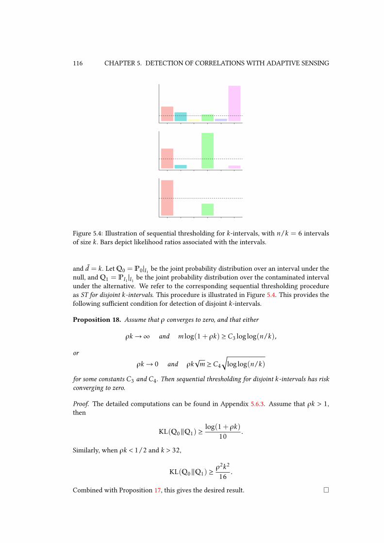
116 CHAPTER 5. DETECTION OF CORRELATIONS WITH ADAPTIVE SENSING
Figure 5.4: Illustration of sequential thresholding for k-intervals, with n/k = 6 intervals
of size k. Bars depict likelihood ratios associated with the intervals.
and d = k. Let Q0 = P0|I1 be the joint probability distribution over an interval under the
null, and Q1 = PI1 |I1 be the joint probability distribution over the contaminated interval
under the alternative. We refer to the corresponding sequential thresholding procedure
as ST for disjoint k-intervals. This procedure is illustrated in Figure 5.4. This provides the
following sucient condition for detection of disjoint k-intervals.
Proposition 18. Assume that ρ converges to zero, and that either
ρk→∞ and m log(1+ ρk) ≥ C3 loglog(n/k),
or
ρk→ 0 and ρk√m ≥ C4
√loglog(n/k)
for some constants C3 and C4. Then sequential thresholding for disjoint k-intervals has riskconverging to zero.
Proof. The detailed computations can be found in Appendix 5.6.3. Assume that ρk > 1,
then
KL(Q0 ||Q1) ≥log(1+ ρk)
10.
Similarly, when ρk < 1/2 and k > 32,
KL(Q0 ||Q1) ≥ρ2k2
16.
Combined with Proposition 17, this gives the desired result.
5.3. ADAPTIVE TESTS 117
Consider the case where ρk →∞. In that case, omitting constant factors, sequential
thresholding would succeed for m ≥ loglog(n)log(1+ρk)
. Recall that uniform non-adaptive testing
is possible for m ≥ c lognρk . When ρk > log(n) asymptotically, both conditions are trivially
satised form constant, while when ρk < log(n), we already improve upon non-adaptive
tests. In spite of this, the dependence on ρk of our sucient condition when ρk → ∞is logarithmic, while it is only linear for ρk → 0. This may appear surprising, as one
may argue the former case corresponds to a regime where the signal is stronger (and so
the problem should be easier). However, this surprising fact is solely an artifact from the
sequential thresholding procedure, and can be xed through a small modication of the
sensing methodology.
In order to recover the same linear dependence in both cases, we propose to add a
subsampling stage prior to sequential thresholding. This subsampling can be decided be-
fore any data is collected, and thus can be viewed as a non-adaptive aspect of the entire
procedure. Consider the simple subsampling scheme wherein one keeps p coordinates per
interval, for some p ∈ 2, . . . ,k, and measures each p-tuple⌊mnpn/k
⌋=
⌊mkp
⌋times. This
prompts the following question: is there a value of p that allows one to detect more eas-
ily? Dene the p-truncated intervals as Ipj = (j −1)k+1, . . . , (j −1)k+ p for j ∈ [n/k].
Formally, we consider the deterministic sensing strategy Ap = (At) where for t ∈[⌊mkp
⌋],
At =⋃
j∈[n/k]
Ipj .
As this involves one simple testing problem per interval, the diculty of testing is essen-
tially characterized by the KL divergence KL(PAp0 ||P
ApS ) between the distributions under
the null and the alternative. In this section, we make explicit the dependence of PS and pby using the notation P
pS . Consider any xed S ∈ D[k], then the best KL divergence that
can be obtained is
maxp∈2,...,k
KL(PAp0 ||P
ApS
)= max
p∈2,...,k
⌊mkp
⌋∑
t=1
KL(Pp0 ||P
pS)
=
⌊mk
p
⌋max
p∈2,...,kKL(P
p0 ||P
pS),
which is independent of S . Due to nonlinearity in the KL divergence the optimal value of
p is generally dierent than k, as illustrated in Figure 5.5. The optimal p and correspondingoptimal value seem hard to compute analytically, but numerical evidence shows that, for
ρ away from zero, the optimal p is of the order of ρ−1. This observation is sucient for
our purposes, and is formalized below. Remark that when ρk < 1, the optimal value of pis clamped to k.
Equipped with this subsampling stage when ρk→∞, we can now modify the ST for
k-intervals procedure as follows: when ρk → ∞, set m =⌊mkp
⌋, d =
⌈1ρ
⌉, and use only
observations corresponding to d coordinates per interval. We refer to this new procedure
as the modied sequential thresholding for disjoint k-intervals.
Proposition 19. Assume that ρ converges to zero, and that either
ρk→∞ and ρkm ≥ C5 loglog(n/k),

118 CHAPTER 5. DETECTION OF CORRELATIONS WITH ADAPTIVE SENSING
0 0.02 0.04 0.06 0.08 0.1 0.12 0.14 0.16 0.18 0.210
20
30
40
50
60
70
80
90
100
Figure 5.5: Optimal p as a function of ρ, for k = 100
or
ρk→ 0 and ρk√m ≥ C6
√loglog(n/k)
for some constants C5,C6. Then the modied sequential thresholding for disjoint k-intervalshas risk converging to zero.
Proof. We have the following straightforward new lower bound, proved in Appendix 5.6.4.
Although the lower bound appears weaker than previously, this corresponds to a setting
where more measurements can be carried out. When ρk > 1, then, using subsampling
with p =⌈1ρ
⌉,
KL(Pp0 ||P
pS) ≥
1
11.
The sucient condition for ST leads to the result.
The adaptive procedure allows us to obtain a mild dependence on the original dimension
n of the problem. When ρ = o(1/k), this sucient condition almost matches the lower
bound of Corollary 1, while when ρk→∞, the sucient condition is already satised for
m = loglog(n/k).
5.3.3 The Case of k-sets: Randomized Subsampling
In this section, we consider the class Ck of k-sets. In this case, we do not currently know
whether a procedure along the lines of ST can be successfully applied. However, the idea of
subsampling the coordinates can still be used to yield modest but important performance
gains. While for disjoint k-intervals a deterministic subsampling was sucient, this is not
the case for k-sets, where any deterministic subsampling that selects less than about n−kcoordinates cannot have risk converging to zero. For this reason, we consider a randomized
subsampling of the coordinates.
Consider a sample B of⌊2npk
⌋elements drawn without replacement from [n] for some
p ≥ 2. Let θ : R⌊np/k⌋ → 0,1 be the localized squared sum test with ambient dimen-
sion⌊2npk
⌋, and contaminated sets C = C⌊p⌋ of size ⌊p⌋, and consider the sensing strategy
dened by
A1 = . . .= A⌊mk2p
⌋= B.

5.3. ADAPTIVE TESTS 119
We refer to the adaptive sensing procedure ((At),θ) as the randomized testing procedure.
Dene Y = |B ∩ S | (resp. Y = 0) under the alternative with contaminated S ∈ Ck (resp.under the null), which is the number of contaminated elements in the subsample. ClearlyY
is a hypergeometric random variable with expectation kn
⌊2nk p
⌋∈ [2p−k/n,2p]. In words,
we consider a subsample of the coordinates, with about 2p contaminated coordinates (in
expectation) under the alternative, and we apply the (non-adaptive) localized squared sum
test.
Note that the procedure is strictly non-adaptive, as the subsampling can be decided in
advance. However, this sensing strategy is a bit dierent than uniform sensing, as not all
coordinates are measured. Nonetheless, this allows one to detect under weaker conditions
than with uniform non-adaptive sensing when k is large enough.
Proposition 20. Let 2 ≤ p ≤ k such that p goes to innity. Assume that ρ converges to zero
and that
ρmk ≥ C1[1− 1
m − 1k
] log 2pn
k, and ρ
√mk ≥ C1√
(p − 1)[1− 1
m − 1k
]
√log
2pn
k,
for some constant C1, then the randomized testing procedure has risk converging to zero.
Proof. Let ηI (resp. ηII ) be the risk of type I (resp. of type II) for θ. The type I error of
the randomized testing procedure is pI = ηI . Let p+ = P(Y ≥ ⌊p⌋) the probability of the
sample containing at least ⌊p⌋ contaminated elements, and p− = 1 − p+. Note that since2npk
kn = 2p goes to innity, we can assume that Y is distributed according to a Poisson
distribution with parameter 2p, as this is asymptotically equivalent to the hypergeomet-
ric distribution. Hence, we have p− = P(Y < ⌊p⌋) ≤(1+
p(2p)p
p!
)exp(−2p). Using p! ≥
√2πp
(pe
)p, we have that p− ≤ exp(−2p)+√p exp(−p/4), which converges to zero. The
type II error of the randomized testing procedure is pII = p+ηII + p−(1−ηI ) ≤ ηII + p−.It remains to show that ηI and ηII both go to zero. This follows from the sucient con-
ditions for the localized squared sum test, and from ⌊p⌋⌊mk2p
⌋≥ mk
2
[1− 1/p+
2(1−p)mk
]≥
mk2 [1− 1/p − 1/m]. Hence, the sucient conditions for the localized squared sum test θprovides the result.
In particular, for p = loglogn, it is sucient that, omitting constants,
ρmk ≥ logn
k, ρ√mk ≥
√log
n
k,
to ensure the detection risk converges to zero. This does not match the adaptive lower
bound, and the dependence on n is still logarithmic. However, this already improves upon
the setting of uniform non-adaptive sensing when k ≥ mlogn . Indeed, recall that using
uniform sensing, the sucient condition is
ρ√mk ≥
√logn, ρm ≥ logn.
The rst condition is insensitive to subsampling, due to the dependence inmk, and we donot improve with respect to it. The second condition, however, only depends on m, and
120 CHAPTER 5. DETECTION OF CORRELATIONS WITH ADAPTIVE SENSING
does not get easier to satisfy when k is large. Hence, our result shows that it is more e-
cient when k is large enough to reduce to a problemwith an almost constant contaminated
set size, but with an increased budget of full vector measurements.
5.4 Unnormalized Correlation Model
5.4.1 Model and Extensions of Previous Results
An alternative choice to the previous correlation model is the following unnormalized
model with covariance matrix
(ΣS)i,j =
1, i = j , i < S ,
1+ ρ, i = j , i ∈ S ,ρ, i , j , and i, j ∈ S ,0 otherwise.
under the alternative with contaminated set S ∈ C. This model is a special case of the rank
one spiked covariance model introduced in (Johnstone, 2001). Observe that this correlation
model can also be rewritten as
H0 : Xti = Y ti , i ∈ 1, . . . ,n,
H1 : Xti =
Y ti , i < S ,
Y ti +√ρN t , i ∈ S for some S ∈ C.
with (Y ti ),Nt independent standard normals. This can thus be interpreted as a random ad-
ditive noise model, as for the model of Section 5.1.1. Observe that our original correlation
detection model is obtained by normalizing each component such that the components
have unit variance. This is a minor dierence that does not essentially change the di-
culty of detection in the non-adaptive setting (indeed all upper and lower bounds proved
in (Arias-Castro et al., 2014) can be reproved for this model with minor modications).
Interestingly, however, under adaptive sensing the information provided by the higher
variance in the contaminated components can be exploited to give a major improvement
over the normalized model. This may be done by applying the sequential thresholding
algorithm to the squares of the components as described below.
In the following, for any quantity X relative to the normalized model of Section 5.1.1,
we denote by X the corresponding quantity related to the unnormalized model. All of
previous results can be shown to hold for this model as well. As already mentioned, this
includes the necessary and sucient conditions of (Arias-Castro et al., 2014) (Proposition
26 in Appendix), but also the lower bound of Theorem 2 (Proposition 27 in Appendix), and
sucient conditions for k-sets and k-intervals of Propositions 20 and 19 (Proposition 29
in Appendix). In particular, the procedures associated to the sucient conditions can be
used with little modications.
5.4.2 The Case of k-sets
The procedure proposed below combines randomized subsamplingwith sequential thresh-
olding, in order to capitalize on the unnormalized model. Consider the second moments
5.4. UNNORMALIZED CORRELATION MODEL 121
Yi = X2i . Under the alternative with contaminated set S ∈ C, Yi is distributed as follows:
(a) for i < S , Yi is distributed according to a chi-squared distribution with one degree of
freedom (that we denote by χ21), (b) for i ∈ S , Yi is distributed as (1+ρ)χ2
1. Note that un-
der our sensing model, it is perfectly legitimate to sampleA1 = 1, . . . ,An = n, and thusobtain independent samples of each of the coordinates of the random vector. In particular,
this allows us to obtain independent samples from the coordinates of Y . As a consequence,we can directly apply ST to detect increased variance over a subset of the coordinates.
As alreadymentioned, ST does not require knowledge of k, which results in a sucient
condition that is independent of k. In particular, it does not become easier to satisfy as
k increases. This condition can, however, be signicantly weakened using the random
subsampling used in last section. As in Proposition 20, this is due to the fact that by
subsampling, one can increase the budget of full vector measurements, while the decrease
in the contaminated set size does not impact the sucient condition for detection. This is
summarized in the following result, which can be proved similarly as Proposition 20.
Proposition 21 (Sucient condition for ST+randomized subsampling). Assume k/n→ 0,
and
liminfn→∞
mkKL(f0 || f1)(loglog2 n)
2> 1,
then the sequential thresholding procedure with randomized subsampling (p = loglog2 n)and a budget of 4m full vector measurements has risk tending to zero as n goes to innity.
Let n = n, k = k, and m =m. Let Q0 be the χ21 distribution, and Q1 be the (1+ρ)χ
21
distribution, both with respect to Lebesgue’s measure. We consider the associated sequen-
tial thresholding procedure (with randomized subsampling), with the previous modica-
tion of sampling independent single coordinates. We refer to this procedure as variance
thresholding. This leads to the following sucient condition for detection.
Proposition 22. Assume that ρ converges to zero and that
ρ√km ≥ C2 loglog2n
for some constant C2. Then, the risk of the variance thresholding procedure converges to zero.
Proof. Let g be the density of a χ21-distributed random variable, such that the density of
a (1 + ρ)χ21-distributed random variable is given by 1
1+ρg( ·1+ρ
). Then, using g(x) ∝
x−1/2e−x/2,
KL(χ21 || (1+ ρ)χ2
1) =
∫
R
log
g(x)1
1+ρg(
x1+ρ
)
g(x)dx
= log(1+ ρ) +
∫
R
log
x−1/2e−x/2
(x
1+ρ
)−1/2e
−x2(1+ρ)
g(x)dx
= log(1+ ρ) +
∫
R
log
e−ρx
2(1+ρ)
(1+ ρ)1/2
g(x)dx
=log(1+ ρ)
2− ρ
2(1+ ρ)
∫
R
xg(x)dx.

122 CHAPTER 5. DETECTION OF CORRELATIONS WITH ADAPTIVE SENSING
As the expectation of a χ21-distributed random variable is one, this leads to
KL(χ21 || (1+ ρ)χ2
1) =1
2
[log(1+ ρ)− ρ
1+ ρ
]=ρ2
4+ o(ρ2).
Plugging this expression into the sucient condition of Proposition 21 provides the result.
Assume for the following discussion that ρk→ 0. The necessary condition that we have
established previously is that ρk√m goes to innity. Neglecting the double log factor,
the sucient condition that we have just obtained is that ρkm goes to innity, which is
stronger. Hence, there is a gap between the sucient and necessary condition. In par-
ticular, that ρk√m goes to innity was shown to be near-sucient for detection with
k-intervals, and the gap that we observe for k-sets does not allow us to conclude as to
whether structure helps for detection (as is the case under non-adaptive sensing).
Recall that the unnormalized model is similar to that of detection in the problem of
sparse PCA. The method of diagonal thresholding (also referred to as Johnstone’s diagonal
method) is a simple and tractable method for detection (and support estimation) in sparse
PCA (with uniform non-adaptive sensing), which consists in testing based on the diag-
onal entries of empirical covariance matrix - that is, the empirical variances. Hence, it
is similar to the method that we consider here, except that we estimate variances based
on independent samples for each coordinate. Note that this last point is essential to our
method. Indeed, consider the opposite case where we do not use independent samples for
each coordinates. For the sake of illustration, assume ρ = 1, such that the contaminated
components are exactly equal. In this case, the probability of throwing away one com-
ponent is equal to that of throwing away all contaminated components, and failure will
occur with xed non small probability due to the use of dependent samples.
Finally, it is noteworthy that a naïve implementation of the optimal test in the non-
adaptive setting has complexityO(nk), whilewith adaptive sensing, we obtain a procedurethat can be carried out in time and space linear in n, and still improves signicantly with
respect to the non-adaptive setting.
5.5 Discussion
We showed that for k-intervals, adaptive sensing allows one to reduce the logarithmic
dependence in n of sucient conditions for non-adaptive detection to a mild loglogn,and that this is near-optimal in a minimax sense.
For k-sets, the story is less complete. The sucient condition obtained in the unnor-
malized model is still stronger than the sucient condition obtained for k-intervals, anddoes not match our common lower bounds, which leaves open the question of whether
structure helps under adaptive sensing for detection of correlations? The analogous question
for detection-of-means has a negative answer, meaning structure does not provide addi-
tional information for detection. However, for detection-of-correlations a denite answer
is still elusive. Another open question is to what extent adaptive sensing allows one to
overcome the exponential computational complexity barrier that one can encounter in the
non-adaptive setting.
Aside from the normalized and unnormalized correlation models, other types of mod-
els can be considered. A more general version of our normalized model has been analyzed

5.5. DISCUSSION 123
in (Arias-Castro et al., 2014), where the correlations need not be all the same, leading to
results that involve the mean correlation coecient ρavg =(∑
i,j∈S : i,j(ΣS)i,j)
/k(k −1).In addition, we assume in most procedures that ρ and/or k are known, and it would be of
interest to have procedures that do not require such knowledge.

124 CHAPTER 5. DETECTION OF CORRELATIONS WITH ADAPTIVE SENSING
5.6 Proofs
5.6.1 Inequalities and KL Divergences
In this section, we collect elementary inequalities that we use repeatedly in the computa-
tions.
For x > −1, log(1+ x) ≤ x, (5.3)
For x > 0, log(1+ x) +1
1+ x− 1 ≤ x2, (5.4)
For 0 < x < 1/2, log(1− x) + 1
1− x − 1 ≤ 2x2, (5.5)
For x < 1, − log(1− x)− 1
1− x + 1 ≤ x2, (5.6)
For x ∈]− 1,1], log(1+ x) +1
1+ x− 1 ≥ x
2
8, (5.7)
For x ≥ 1, log(1+ x) +1
1+ x− 1 ≥ log(1+ x)
5. (5.8)
The following expression of the KL divergence is used throughout the chapter.
Proposition 23. We have
KL(P0 ||PS) =1k≥22
[k
(−1+ 1
1− ρ + log(1− ρ))−(
1
1− ρ + log(1− ρ))
(5.9)
+
(1
1+ ρ(k − 1) + log(1+ ρ(k − 1)))].
Proof. The KL divergence betweenP0 andPS can be computed using the standard formula
for KL divergence between two centered Gaussian vectors, with covariance matrices
Σ0 = In, Σ1 = ΣS .
When k < 2, the divergence is zero, and we will thus assume k ≥ 2. Up to a simultaneous
permutation of rows and columns,
ΣS =
[In−k
Jρ(k)
]
where Jρ(k) ∈ Rk×k has unit diagonal and coecients equal to ρ everywhere else. Jρ(k)is a symmetric matrix, hence diagonalizable, and has eigenvalues 1 − ρ with multiplicity
k − 1 and 1+ (k − 1)ρ with multiplicity one. As a consequence, we have, for k ≥ 2,
logdetΣS = (k − 1) log(1− ρ) + log(1+ ρ(k − 1))
TrΣ−1S = (n− k) + k − 11− ρ +
1
1+ ρ(k − 1) .

5.6. PROOFS 125
The KL divergence is thus
KL(P0 ||PS)
=1
2
[Tr(Σ−11 Σ0)−n− log(detΣ0/detΣ1)
]
=1
2
[(n− k) + k − 1
1− ρ +1
1+ ρ(k − 1) −n+ (k − 1) log(1− ρ) + log(1+ ρ(k − 1))]
=1
2
[k
(−1+ 1
1− ρ + log(1− ρ))−(
1
1− ρ + log(1− ρ))
+
(1
1+ ρ(k − 1) + log(1+ ρ(k − 1)))].
5.6.2 Proof of Bound on KL Divergence
Proof. First note since the KL divergences are independent of n, it is sucient to use the
expressions of Proposition 23with a contaminated set of size s = |A∩S | ≤ k. As previously,we assume s ≥ 2, as the result is trivial otherwise. Consider the expression for the KL
divergence given in (5.9). Using (5.3), we obtain
KL(P0|A ||PS |A)= KL(P0 ||PS∩A)
≤ 1
2
[s
(−1+ 1
1− ρ + log(1− ρ) + ρ
)−(
1
1− ρ + log(1− ρ))+
(1
1+ ρ− ρ
)]
=1
2
[s
(ρ+
ρ
1− ρ + log(1− ρ))+−2ρ1− ρ2 − log(1− ρ)− ρ
]
≤ ρs
2(1− ρ) .
Using (5.4) and (5.6), we obtain
KL(P0 ||PS) ≤1
2
[(s − 1)2ρ2+ 2sρ2+ ρ2
]=ρ2
2
[(s − 1)2+ 2s+ 1
]≤ ρ
2s(k+ 1)
2.
5.6.3 Proof of Proposition 18
Proof. We have KL(Q0 ||Q1) = kf (ρ) + h(ρ) with
f (ρ) =1
2
[(1− ρ)−1+ log(1− ρ)− 1
],
h(ρ) =1
2
[−(
1
1− ρ + log(1− ρ))+
(1
1+ (p − 1)ρ + log(1+ (p − 1)ρ))].

126 CHAPTER 5. DETECTION OF CORRELATIONS WITH ADAPTIVE SENSING
As previously, using (5.7), f (ρ) ≥ ρ2
16 . Assume that ρk < 1 and k > 7, then using (5.5) and
(5.7),
KL(Q0 ||Q1) ≥ρ2k
16+ h(ρ)
≥ ρ2k
16− 1
2
[1+ 2ρ2
]+
1
2
[1+
ρ2(k − 1)28
]
= ρ2[k(k − 1)2
16− 1
]
≥ (ρk)2
32.
Now assume that ρk > 1, then for k > 32,
KL(Q0 ||Q1) ≥ρ2k
16− 1
2
[1+ 2ρ2
]+
1
2
[1
1+ (k − 1)ρ + log(1+ (k − 1)ρ)]
≥ ρ2[k
16− 1
]+
1
2
[1
1+ (k − 1)ρ + log(1+ (k − 1)ρ)− 1]
≥ ρ2k
32+
log(1+ (k − 1)ρ)− 12
.
5.6.4 Proof of Proposition 19
Proof. With p =⌈1ρ
⌉, when ρk > 1, we have
⌈1ρ
⌉< k+ 1, and as a consequence,
KL(Pp0 ||P
pS) ≥
log2− 1/2
2≥ 1
11.

5.7. APPENDIX: EXTENSIONS TO UNNORMALIZED MODEL 127
5.7 Appendix: Extensions to Unnormalized Model
5.7.1 Uniform (non-adaptive) Lower Bound
Proposition 24. For any class C, any ρ ∈ [0,0.9), the minimum risk in the normalized
model (resp. the unnormalized model) under uniform (non-adaptive) sensing is bounded as
R∗ ≥ 1
2− 1
4
√
E
[coshm
(8ρZ
1− ρ
)]− 1
R∗ ≥ 1
2− 1
4
√E [coshm (8ρZ)]− 1
whereZ is the size of the intersection of two elements of C drawn independently and uniformly
at random.
Proof. This is essentially a reproduction of the proof of (Arias-Castro et al., 2014) with
minor modications. The details are omitted.
5.7.2 Uniform (non-adaptive) Upper Bound
Let H(b) = b − 1− logb for b > 1.
Proposition 25. Under uniform (non-adaptive) sensing, the localized square-sum test that
rejects when
Yscan =maxS∈C
m∑
t=1
∑
i∈SXti
2
exceeds1
2
(ρk2m+H−1(3log |C|/m)− 1)km
)
is asymptotically powerful when
ρk ≥ c1max
√log |C|m
,log |C|m
both for the normalized and unnormalized models.
Proof. This is proved in (Arias-Castro et al., 2014) for the normalized model. In the case
of the unnormalized model, the test statistic is distributed as kχ2m under the null, and as
(k(1+ρ)+ρk(k−1))χ2m under the alternative, which changes only mildly the proof with
respect to the normalized model.
5.7.3 KL Divergences
Proposition 26. We have
KL(P0 || PS) =1k≥22
[−1+ 1
1+ ρk+ log(1+ ρk)
]. (5.10)
128 CHAPTER 5. DETECTION OF CORRELATIONS WITH ADAPTIVE SENSING
Proof. The KL divergence between P0 and PS can be computed using the standard formula
for KL divergence between two centered Gaussian vectors, with covariances matrices
Σ0 = In, Σ1 = ΣS .
When k = 0, the divergence is zero, and we will thus assume k ≥ 1. Up to a simultaneous
permutation of rows and columns,
ΣS =
[In−k
Ik +Kρ(k)
]
where Kρ(k) ∈ Rk×k has coecients equal to ρ everywhere. Like previously, Ik +Kρ(k)is diagonalizable, and has eigenvalue 1with multiplicity k−1, and eigenvalue 1+ρk withmultiplicity one. As a consequence, for k ≥ 1, we have
logdet ΣS = log(1+ ρk)
Tr Σ−1S = (n− 1) + 1
1+ ρk.
This leads to
KL(P0 || PS) =1
2
[Tr(Σ−11 Σ0)−n− log(detΣ0/detΣ1)
]
=1
2
[(n− 1)−n+ 1
1+ ρk+ log(1+ ρk)
].
Proposition 27. For any A ⊂ [n],
KL(P0|A || PS |A) ≤min
[ρ
2,ρ2k
2
]|A∩ S |.
Proof. First note since the KL divergences are independent of n, it is sucient to use the
expressions of Proposition 23 with a contaminated set of size s = |A∩ S |. As previously,we assume s ≥ 1, as the result is trivial otherwise. Consider the unnormalized model, with
KL divergence given in (5.10). Using (5.3), we obtain
KL(P0|A || PS |A) = KL(P0 || PA∩S) ≤ρs
2.
Using (5.4) we obtain
KL(P0|A || PS |A) = KL(P0 || PA∩S) ≤ρ2s2
2≤ ρ
2sk
2.
Combining these last two inequalities yields the desired result.
Proposition 28. Assume that ρ converges to zero, and that either
ρk→∞ and m log(1+ ρk) ≥ C3 loglog(n/k),
or
ρk→ 0 and ρk√m ≥ C4
√loglog(n/k)
for some constants C3 and C4. Then sequential thresholding for disjoint k-intervals has riskconverging to zero.

5.7. APPENDIX: EXTENSIONS TO UNNORMALIZED MODEL 129
Proof. For the unnormalized model, when ρk > 1, using (5.8),
KL(Q0 ||Q1) ≥log(1+ ρk)
10.
When ρk < 1, using (5.7),
KL(Q0 ||Q1) ≥(ρk)2
16.
Proposition 29. Assume that ρ converges to zero, and that either
ρk→∞ and ρkm ≥ C5 loglog(n/k),
or
ρk→ 0 and ρk√m ≥ C6
√loglog(n/k)
for some constants C5,C6. Then the modied sequential thresholding for disjoint k-intervalshas risk converging to zero.
Proof. For the unnormalized model with p =⌈1ρ
⌉, when ρk > 1, we have
⌈1ρ
⌉< k+ 1, and
as a consequence,
KL(Pp0 || P
pS) ≥
log2− 1/2
2≥ 1
11.


6Detection of Objects with
High-dimensional CNN Features“I well recall a group of us, after a sessionon the IBM 701 at a meeting where theytalked about the proposed 18 machines, allbelieved this would saturate the market formany years!"
— Richard Hamming
Contents
6.1 Introduction . . . . . . . . . . . . . . . . . . . . . . . . . . . . . . . . . . . 132
6.2 Detection with DPMs . . . . . . . . . . . . . . . . . . . . . . . . . . . . . . 133
6.2.1 Detection Task . . . . . . . . . . . . . . . . . . . . . . . . . . . . . 133
6.2.2 Deformable Part Models . . . . . . . . . . . . . . . . . . . . . . . . 133
6.3 Integrating Convolutional Features into DPMs . . . . . . . . . . . . . . . . 135
6.3.1 The Alexnet Network Structure . . . . . . . . . . . . . . . . . . . . 135
6.3.2 Prior Work . . . . . . . . . . . . . . . . . . . . . . . . . . . . . . . 136
6.3.3 Using CNN Layer 5 Features in DPMs . . . . . . . . . . . . . . . . 137
6.4 Results on Pascal VOC 2007 . . . . . . . . . . . . . . . . . . . . . . . . . . 138
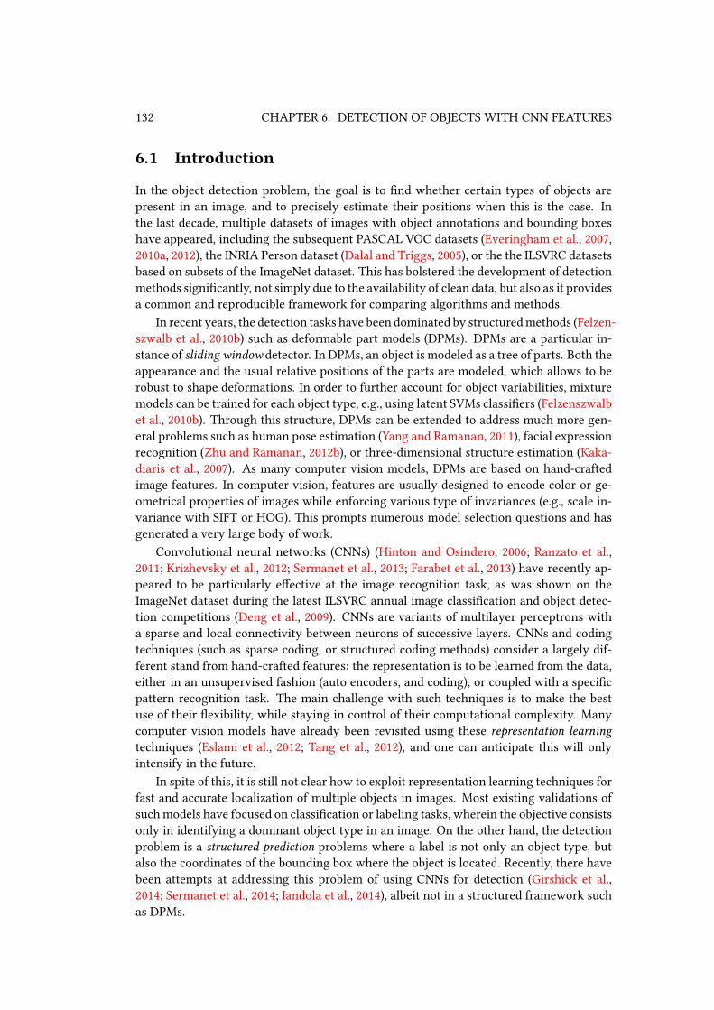
132 CHAPTER 6. DETECTION OF OBJECTS WITH CNN FEATURES
6.1 Introduction
In the object detection problem, the goal is to nd whether certain types of objects are
present in an image, and to precisely estimate their positions when this is the case. In
the last decade, multiple datasets of images with object annotations and bounding boxes
have appeared, including the subsequent PASCAL VOC datasets (Everingham et al., 2007,
2010a, 2012), the INRIA Person dataset (Dalal and Triggs, 2005), or the the ILSVRC datasets
based on subsets of the ImageNet dataset. This has bolstered the development of detection
methods signicantly, not simply due to the availability of clean data, but also as it provides
a common and reproducible framework for comparing algorithms and methods.
In recent years, the detection tasks have been dominated by structuredmethods (Felzen-
szwalb et al., 2010b) such as deformable part models (DPMs). DPMs are a particular in-
stance of sliding window detector. In DPMs, an object is modeled as a tree of parts. Both the
appearance and the usual relative positions of the parts are modeled, which allows to be
robust to shape deformations. In order to further account for object variabilities, mixture
models can be trained for each object type, e.g., using latent SVMs classiers (Felzenszwalb
et al., 2010b). Through this structure, DPMs can be extended to address much more gen-
eral problems such as human pose estimation (Yang and Ramanan, 2011), facial expression
recognition (Zhu and Ramanan, 2012b), or three-dimensional structure estimation (Kaka-
diaris et al., 2007). As many computer vision models, DPMs are based on hand-crafted
image features. In computer vision, features are usually designed to encode color or ge-
ometrical properties of images while enforcing various type of invariances (e.g., scale in-
variance with SIFT or HOG). This prompts numerous model selection questions and has
generated a very large body of work.
Convolutional neural networks (CNNs) (Hinton and Osindero, 2006; Ranzato et al.,
2011; Krizhevsky et al., 2012; Sermanet et al., 2013; Farabet et al., 2013) have recently ap-
peared to be particularly eective at the image recognition task, as was shown on the
ImageNet dataset during the latest ILSVRC annual image classication and object detec-
tion competitions (Deng et al., 2009). CNNs are variants of multilayer perceptrons with
a sparse and local connectivity between neurons of successive layers. CNNs and coding
techniques (such as sparse coding, or structured coding methods) consider a largely dif-
ferent stand from hand-crafted features: the representation is to be learned from the data,
either in an unsupervised fashion (auto encoders, and coding), or coupled with a specic
pattern recognition task. The main challenge with such techniques is to make the best
use of their exibility, while staying in control of their computational complexity. Many
computer vision models have already been revisited using these representation learning
techniques (Eslami et al., 2012; Tang et al., 2012), and one can anticipate this will only
intensify in the future.
In spite of this, it is still not clear how to exploit representation learning techniques for
fast and accurate localization of multiple objects in images. Most existing validations of
suchmodels have focused on classication or labeling tasks, wherein the objective consists
only in identifying a dominant object type in an image. On the other hand, the detection
problem is a structured prediction problems where a label is not only an object type, but
also the coordinates of the bounding box where the object is located. Recently, there have
been attempts at addressing this problem of using CNNs for detection (Girshick et al.,
2014; Sermanet et al., 2014; Iandola et al., 2014), albeit not in a structured framework such
as DPMs.

6.2. DETECTION WITH DPMS 133
In this work, we demonstrate that using CNN feature pyramids within DPMs allows
to obtain a signicant boost in DPM performance on VOC2007. In Section 6.2, we review
the object detection problem and the DPM framework. In Section 6.3, we look at CNNs,
and describe how such feature representations can be integrated with DPMs. Finally, we
present experimental results on VOC2007 in Section 6.4, and we close this chapter with a
discussion of the results in Section ??. This chapter is joint work with Iasonas Kokkinos
and Stavros Tsogkas.
6.2 Detection with DPMs
In this section, we review the detection task, and give a high-level overview of DPMs.
6.2.1 Detection Task
In computer vision, the detection task consists in both identifying the types of the objects
in an image, and precisely localizing them. Detection results are usually evaluated based
on the following measure of overlap between a predicted bounding box, and an annotated
bounding box. The Intersection over Union (IoU, also referred to as Jaccard’s coecient) of
two bounding boxes B1 = xmin1 , . . . ,xmax
1 × ymin1 , . . . ,ymax
1 and B2 = xmin2 , . . . ,xmax
2 ×ymin
2 , . . . ,ymax2 is
IoU(B1,B2) =|B1 ∩B2||B1 ∪B2|
.
In the PASCAL VOC detection challenges (Everingham et al., 2007), a predicted bounding
box for a given class is considered a true positive if the best IoU with a ground truth
bounding box for this class exceeds 0.5. A given ground truth bounding box can only be
used for a single predicted bounding box, such that predicting many close bounding boxes
leads to many false positives. Predictions are required to be accompanied by a condence
score, such that a varying threshold can be used to explore dierent detection regimes. The
nal evaluation is in terms of precision/recall curve, which is usually summarized with the
average precision (AP, the area under the precision/recall curve). The high recall regime
corresponds to many bounding box predictions thus capturing all the objects, while the
high precision regime corresponds to a small number of relevant bound box predictions.
Understanding failures of detectors is paramount to improve their performance. In
detection, errors can be of dierent types. Localization errors correspond to where an
object was correctly detected, but poorly localized so that the IoU does not exceed the
threshold (this includes duplicate detections). False positives can be classied (Hoiem et al.,
2012) into confusion with similar objects, confusion with dissimilar objects, or confusion
with background. This is illustrated in Figure 6.1.
6.2.2 Deformable Part Models
In this section, we review star-shaped deformable part models. These models are dened
by a root node which models the global appearance of the object, and part nodes which
are allowed to oat around the position of the root node to model certain specic features
of the object. As a simple example, the problem of human pose estimation can be cast as
such a star-shaped DPM, with parts for the head, the torso, the arms, and the legs. A given
bounding box is scored in DPMs according to the score of the root model, of the parts

134 CHAPTER 6. DETECTION OF OBJECTS WITH CNN FEATURES
bottle (loc): ov=0.30 1−r=0.98 bottle (bg): ov=0.00 1−r=0.98
Figure 6.1: Localization error (left), confusion with background (right)
models, and of the value of interaction terms between the root and the parts. When train-
ing in the absence of precise annotation for the parts, their positions are treated as latent
variables, and are estimated. When doing detection, the score of a bounding box corre-
sponds to the highest scoring conguration over all possible parts locations. Examples of
detections along with the latent part locations are shown in Figure 6.2.
Figure 6.2: Part basedmodels, sample detections from Felzenszwalb et al. (2010b): detection
bounding box (red), latent parts (blue)
Formally, DPMs associate linear lters with the root and the part nodes. The part
lters are usually square lters of xed size, while the root lters are larger. Consider a
root-part conguration z = (z0,z1, . . . zP) , where z0 is the image location of the center of
the root lter, while, z1, . . . ,zP are the image locations of the centers of each of the part
lters. Denote by I(z) a feature representation of the image patch around image location
z, of size corresponding to that of the root lter or of the part lters, depending on context.A conguration is scored using a model of the form
M(z) = 〈w0, I(z0)〉+P∑
p=1
[〈wp, I(zp)〉+Bp(zp,z0)
].
Here, w0,w1, . . . ,wP are the lters (in feature space), and the dot product describes how
well the patch at this position matches the part model. The terms Bp are the second orderpotentials, and depend only on the relative position dierence zp − z0. For instance, in
the case of human pose estimation, one may want to penalize when the head part is not

6.3. INTEGRATING CONVOLUTIONAL FEATURES INTO DPMS 135
strictly above the torso, or when the left arm is not to the left of the torso. These terms
are usually simple quadratic forms. At training time, both the lters w1, . . . ,wP and the
second order potentials B1, . . . ,BP must be learned.
Using this model, bounding box predictions can be produced as follows. First, we
decide on an aspect ratio and a putative root lter location z0, that leads to a candidate
bounding box. The best score over all compatible part congurations is
S(z0) = maxz :z0=z0
M(z).
This provides a condence score. Finally, this procedure is actually used for all possible
root positions z0, which justies that DPMs are referred to as dense detectors. For this rea-
son, DPMs may be slow both to train and to evaluate. However, DPMs can be accelerated
signicantly at test time using cascades (Felzenszwalb et al., 2010a), branch and bound
(Kokkinos, 2011), or score approximations (Kokkinos, 2013).
The procedure that we have described can be used to detect objects at a xed scale
that depends on the size of the part and of the root lters. In order to detect objects at all
scales, a feature pyramid is used instead of a simple single-scale feature representation of
the image. At an elementary level, this is equivalent to performing detection on rescaled
version of a single image. This is illustrated on Figure 6.3: down-sampled versions of
the image may allow to detect the head of the horse, while higher resolutions may allow
to detect ner details such as the ears of the horse. In addition, a mixture of such models
can be considered, leading to an additional latent variable which is the mixture component
identier. Thesemixture components allow to account for dierent viewpoints or subtypes
of objects within a given class. In particular, root lters with dierent aspect ratios are
traditionally used.
6.3 Integrating Convolutional Features into DPMs
In this chapter, we consider the core problem of this chapter: how canwe use features from
CNNs for detection with DPMs, instead of using HOG features or similar hand-crafted
representations? In the remainder of this section, we go into detail into the structure of
the CNN that we consider, as well as into practical details for integrating deep features
into DPMs.
6.3.1 The Alexnet Network Structure
Most of recent works with CNNs for image classication or object detection are focused on
the Alexnet network (Krizhevsky et al., 2012), which has won recent ImageNet object clas-
sication challenges. The Alexnet name is used both to refer to the network structure (i.e.,
the number, shapes and types of layers), and to refer to already-trained networks based on
this structure. The rst ve layers are convolutional, and consist only of convolutions and
pooling layers. Hence, the rst ve layers are intrinsically translation equivariant. The
last two layers are classical fully connected layers as in multi-layer perceptrons. The input
of the network consists of a 224×224×3 patch, which is transformed to two 13×13×128patches after layer 5, and to a 4096 dimensional vector after layer 7. While the features
obtained at the convolutional layers have a spatial interpretation (as is the case with HOG),
this is not the case at the fully-connected layers.

136 CHAPTER 6. DETECTION OF OBJECTS WITH CNN FEATURES
Figure 6.3: Feature pyramid: original image at dierent scales (left), energy of CNN feature
representation at layer 5 (right)
The Alexnet network was trained on the ImageNet database, where all images were
rescaled to a xed size, and the mean of all these images was subtracted. In order to
augment the data for training, random translations and horizontal reections were used,
and have been observed to reduce over-tting. However, the Alexnet network was trained
for classication, and it may be benecial to retrain the networkwhenworking on a related
but dierent task such as detection, as was observed for R-CNN, where this is referred to as
ne-tuning (Girshick et al., 2014). This can be achieved by setting up a supervised objective
adapted to the task at hand, and performing back-propagation on the original network.
6.3.2 Prior Work
An interesting attempt at using CNNs for detection has been made with OverFeat (Ser-
manet et al., 2014), which considers a sliding window approach. Two CNNs are jointly
trained to predict the class of the object and the coordinates of the bounding box contain-
ing the object, respectively, from a given input window. These networks are then fed with
all possible windows from the original images, at dierent scales. A squared loss is used
as the loss for the bounding box regression problem.
The Regions with CNN features (R-CNN) method (Girshick et al., 2014) addresses the
detection problem in a remarkably simple and eective way, through the use of region
proposals (Uijlings et al., 2013). Many promising regions are obtained from segmentation
considerations and warped to a xed size window, which is then used as input to a CNN.
This is essentially a reduction to a classication task, but performs extremely well, pro-

6.3. INTEGRATING CONVOLUTIONAL FEATURES INTO DPMS 137
viding a mean average precision (mAP) of 58.5% on 20-classes VOC2007, and of 31.4% on
200-classes ILSVRC2013. These large mAPs are at the expense, however, of the time spent
training and testing: even though the method scales well with the number of classes, the
computation of the CNN features over all warped region proposals is expensive, even on
modern GPU machines. In addition, R-CNN is not a structured detector, and hence cannot
be generalized easily to more dicult structure estimation problems.
6.3.3 Using CNN Layer 5 Features in DPMs
Due to translational equivariance, the output of the convolutional layers can actually be
computed on images larger than the input patch size used for training. This was lever-
aged in OverFeat (Sermanet et al., 2014) and in other recent works (Iandola et al., 2014;
He et al., 2014). In particular, Iandola et al. (2014) proposed to compute a feature pyramid
based on the convolutional layers (i.e., using the layer 5 features of the network). In or-
der to obtain a multi-scale representation, the patchwork of scales approach (Dubout and
Fleuret, 2012) is used: dierent scales of an image are stitched in a large patchwork image
as shown in Figure 6.4, and the feature representation of the patchwork image is computed
and transformed back into a pyramid. This work demonstrates how to compute feature
pyramids based on a convolutional network, but no quantitative evaluation on a specic
task is provided.
Figure 6.4: Patchwork method: original stitched image (left), energy of CNN feature rep-
resentation at layer 5 (right)
However, a full image cannot be directly propagated through the fully-connected lay-
ers, which require a xed size input that has to be xed at the time where the network
is trained. From a feature pyramid at layer 5, one may crop (or warp to) patches of xed
size to compute the output of the fully-connected layers (He et al., 2014), or simply stick
to the spatially arranged features at layer 5. This is in contrast with the approach used in
R-CNN which rst warps to a xed size before even the convolutional layer. In order to
have a structured detector like with DPMs, we need to conserve a spatial arrangement of
the features, as this allows to share computations when scoring part congurations. As
a consequence, we choose in this work to directly use the feature pyramid based directly
upon the layer 5 features.
When extracting such features, a key quantity is the subsampling factor sub from the
original input to the spatial feature representation, also referred to as the bin size, as il-
lustrated in Figure 6.5. For Alexnet, sub = 16, such that each feature is computed over
16×16 cells over the input image. As this corresponds to large bins, we oversampled by a
factor of two all images before computing features, which eectively leads to sub= 8. We
note that in Figure 6.3, the features have been resized by a factor of sub in order to appear
of the same size as the images. Figure 6.5 illustrates this with sub = 16: each pixel in the

138 CHAPTER 6. DETECTION OF OBJECTS WITH CNN FEATURES
feature representation corresponds to a 16× 16 cell in the original image. Higher resolu-
Figure 6.5: Illustration of subsampling factor
tions can be obtained similarly, e.g., sub = 4 can be obtained by oversampling by a factor
of four, although feature computation as well as training and testing become prohibitively
long. The layer 5 features in each bin are 256-dimensional, which is eight times more than
with HOG features, which further increases the computational challenges associated with
training such models.
With HOG, the features can be interpreted as normalized frequencies for orientations
of the gradients, and can thus be represented visually, or even transformed back into the
image domain to some extent (Vondrick et al., 2013). With layer 5 CNN features, this type
of interpretation is not possible. Although we have represented CNN features through
their total energy so far, it would be desirable to have a way to visualize the feature rep-
resentations of the images, as well as the lters.
6.4 Results on Pascal VOC 2007
Instead of the Alexnet network, we use the R-CNN network ne-tuned for detection with
region proposals. We only report results with sub = 8, as sub = 16 leads to signicantly
worse mAPs, while sub = 4 is computationally prohibitive. We consider a normalization
for the CNN feature that is based on the L2-Hys (for hysteresis) scheme (Dalal and Triggs,
2005). Given a feature vector x, normalize in Euclidean norm:
x← x
‖x‖2+ ε,
with ε = 10−3. Then, x is capped componentwise to a maximum value v = 0.1:
x←min(x,v).
We note that the layer 5 features are nonnegative, such that this is equivalent to capping
to a maximum amplitude. Finally, x is normalized again in Euclidean norm. In addition to
L2H-Hys, we investigated other normalization schemes, such as simple Euclidean norm
normalization, or ℓ1-norm normalization. Both of these alternative schemes yielded simi-
lar results.
In DPMs, it is common to train distinct mixture components for left-facing and right-
facing objects. When using HOG features, one may avoid to double the number of linear
classiers by leveraging the fact that the HOG features of a ipped patch can be obtained
by shuing the HOG features of the original patch. This is because HOG features are
dened in terms of the geometrical orientations of the image gradient. Hence, given a
lter for a left-facing object, one may obtain in closed-form a lter for right-facing objects
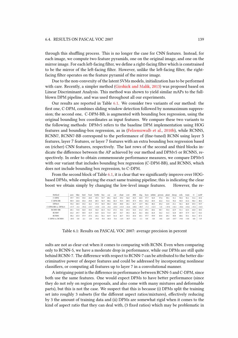
6.4. RESULTS ON PASCAL VOC 2007 139
through this shuing process. This is no longer the case for CNN features. Instead, for
each image, we compute two feature pyramids, one on the original image, and one on the
mirror image. For each left-facing lter, we dene a right-facing lter which is constrained
to be the mirror of the left-facing lter. However, unlike the left-facing lter, the right-
facing lter operates on the feature pyramid of the mirror image.
Due to the non-convexity of the latent SVMsmodels, initialization has to be performed
with care. Recently, a simpler method (Girshick and Malik, 2013) was proposed based on
Linear Discriminant Analysis. This method was shown to yield similar mAPs to the full-
blown DPM pipeline, and was used throughout all our experiments.
Our results are reported in Table 6.1. We consider two variants of our method: the
rst one, C-DPM, combines sliding window detection followed by nonmaximum suppres-
sion; the second one, C-DPM-BB, is augmented with bounding box regression, using the
original bounding box coordinates as input features. We compare these two variants to
the following methods: DPMv5 refers to the baseline DPM implementation using HOG
features and bounding-box regression, as in (Felzenszwalb et al., 2010b), while RCNN5,
RCNN7, RCNN7-BB correspond to the performance of (ne-tuned) RCNN using layer 5
features, layer 7 features, or layer 7 features with an extra bounding box regression based
on (richer) CNN features, respectively. The last rows of the second and third blocks in-
dicate the dierence between the AP achieved by our method and DPMv5 or RCNN5, re-
spectively. In order to obtain commensurate performance measures, we compare DPMv5
with our variant that includes bounding box regression (C-DPM-BB), and RCNN5, which
does not include bounding box regression, to C-DPM.
From the second block of Table 6.1, it is clear that we signicantly improve over HOG-
based DPMs, while employing the exact same training pipeline; this is indicating the clear
boost we obtain simply by changing the low-level image features. However, the re-
Method aero bike bird boat bottle bus car cat chair cow dtbl dog hors mbike person plant sheep sofa train tv mAP
C-DPM 39.7 59.5 35.8 24.8 35.5 53.7 48.6 46.0 29.2 36.8 45.5 42.0 57.7 56.0 37.4 30.1 31.1 50.4 56.1 51.6 43.4
C-DPM-BB 50.9 64.4 43.4 29.8 40.3 56.9 58.6 46.3 33.3 40.5 47.3 43.4 65.2 60.5 42.2 31.4 35.2 54.5 61.6 58.6 48.2
DPMv5 33.2 60.3 10.2 16.1 27.3 54.3 58.2 23.0 20.0 24.1 26.7 12.7 58.1 48.2 43.2 12.0 21.1 36.1 46.0 43.5 33.7
C-DPM-BB vs. DPMv5 +17.7 +4.1 +33.2 +13.7 +13.0 +2.6 +0.4 +23.3 +13.3 +16.4 +20.6 +30.7 +7.1 +12.3 -1.0 +19.4 +14.1 +18.4 +15.6 +15.1 +14.5
RCNN7-BB 68.1 72.8 56.8 43.0 36.8 66.3 74.2 67.6 34.4 63.5 54.5 61.2 69.1 68.6 58.7 33.4 62.9 51.1 62.5 64.8 58.5
RCNN7 64.2 69.7 50.0 41.9 32.0 62.6 71.0 60.7 32.7 58.5 46.5 56.1 60.6 66.8 54.2 31.5 52.8 48.9 57.9 64.7 54.2
RCNN5 58.2 63.3 37.9 27.6 26.1 54.1 66.9 51.4 26.7 55.5 43.4 43.1 57.7 59.0 45.8 28.1 50.8 40.6 53.1 56.4 47.3
C-DPM vs. RCNN5 -18.5 -3.8 -2.1 -2.8 +9.4 -0.4 -18.3 -5.4 +2.5 -18.7 +2.1 -1.1 0.0 -3.0 -8.4 +2.0 -19.7 +9.8 +3.0 -4.8 -3.9
Table 6.1: Results on PASCAL VOC 2007: average precision in percent
sults are not as clear-cut when it comes to comparing with RCNN. Even when comparing
only to RCNN-5, we have a moderate drop in performance, while our DPMs are still quite
behind RCNN-7. The dierence with respect to RCNN-7 can be attributed to the better dis-
criminative power of deeper features and could be addressed by incorporating nonlinear
classiers, or computing all features up to layer 7 in a convolutional manner.
A intriguing point is the dierence in performance between RCNN-5 and C-DPM, since
both use the same features. One would expect DPMs to have better performance (since
they do not rely on region proposals, and also come with many mixtures and deformable
parts), but this is not the case. We suspect that this is because (i) DPMs split the training
set into roughly 3 subsets (for the dierent aspect ratios/mixtures), eectively reducing
by 3 the amount of training data and (ii) DPMs are somewhat rigid when it comes to the
kind of aspect ratio that they can deal with, (3 xed ratios) which may be problematic in

140 CHAPTER 6. DETECTION OF OBJECTS WITH CNN FEATURES
the presence of large aspect ratio variatios; by contrast RCNN warps all region proposals
images onto a single canonical scale. To conclude, we have shown that replacing HOG fea-
tures with CNN features yields a substantial improvement in DPM detection performance;
given the widespread use of DPMs in a broad range of structured prediction tasks (Yang
and Ramanan, 2013; Zhu and Ramanan, 2012a), we anticipate that this will soon become
common practice.

Bibliography
L. Addario-Berry, N. Broutin, L. Devroye, and G. Lugosi. On combinatorial testing prob-
lems. Annals of Statistics, 38:3063–3092, 2010.
A. Agarwal, S. Negahban, M. J. Wainwright, et al. Noisy matrix decomposition via convex
relaxation: Optimal rates in high dimensions. Annals of Statistics, 40(2):1171–1197, 2012.
H. Akaike. A new look at the statistical model identication. IEEE Transactions on Auto-
matic Control, 19(6):716–723, 1974.
F. Alizadeh and D. Goldfarb. Second-order cone programming. Mathematical Program-
ming, 95(1):3–51, 2003.
N. Alon and A. Naor. Approximating the cut-norm via grothendieck’s inequality. SIAM
Journal on Computing, 35(4):787–803, 2006.
D. Amelunxen, M. Lotz, M. B. McCoy, and J. A. Tropp. Living on the edge: A geometric
theory of phase transitions in convex optimization. arXiv preprint arXiv:1303.6672, 2013.
B. P. Ames and S. A. Vavasis. Nuclear normminimization for the planted clique and biclique
problems. Mathematical programming, 129(1):69–89, 2011.
A. A. Amini and M. J. Wainwright. High-dimensional analysis of semidenite relaxations
for sparse principal components. In Information Theory, 2008. ISIT 2008. IEEE Interna-
tional Symposium on, pages 2454–2458. IEEE, 2008.
A. Anandkumar, R. Ge, D. Hsu, S. M. Kakade, and M. Telgarsky. Tensor decompositions
for learning latent variable models. arXiv preprint arXiv:1210.7559, 2012.
A. Argyriou, C. A. Micchelli, and M. Pontil. When is there a representer theorem? vector
versus matrix regularizers. Journal of Machine Learning Research, 10:2507–2529, 2009.
A. Argyriou, R. Foygel, and N. Srebro. Sparse prediction with the k-support norm. In Proc.
NIPS, pages 1457–1465, 2012.
E. Arias-Castro, E. J. Candès, H. Helgason, and O. Zeitouni. Searching for a trail of evidence
in a maze. Annals of Statistics, 36:1726–1757, 2008.
E. Arias-Castro, S. Bubeck, and G. Lugosi. Detection of correlations. Annals of Statistics,
40(1):412–435, 2012.
E. Arias-Castro, E. J. Candes, and M. A. Davenport. On the fundamental limits of adaptive
sensing. IEEE Trans. Information Theory, 59(1):472–481, 2013.
E. Arias-Castro, S. Bubeck, and G. Lugosi. Detecting positive correlations in a multivariate
sample. Bernoulli, 2014.

142 BIBLIOGRAPHY
F. Bach, G. R. G. Lanckriet, and M. I. Jordan. Multiple Kernel Learning, Conic Duality, and
the SMO Algorithm. In Proc. ICML, 2004.
F. R. Bach, R. Thibaux, and M. I. Jordan. Computing regularization paths for learning
multiple kernels. Proc. NIPS, 17:73–80, 2005.
G. Bakir, T. Hofmann, B. Scholkopf, A. Smola, B. Taskar, and S. Vishanathan. Predicting
structured data. MIT Press, 2007.
O. Banerjee, L. El Ghaoui, and A. d’Aspremont. Model selection through sparse maxi-
mum likelihood estimation for multivariate gaussian or binary data. Journal of Machine
Learning Research, 9:485–516, 2008.
Y. Baraud. Non-asymptotic minimax rates of testing in signal detection. Bernoulli, 8:577–
606, 2002.
P. L. Bartlett and S. Mendelson. Rademacher and gaussian complexities: Risk bounds and
structural results. Journal of Machine Learning Research, 3:463–482, 2003.
A. Beck and M. Teboulle. A fast iterative shrinkage-thresholding algorithm for linear
inverse problems. SIAM Journal of Imaging Sciences, 2(1):183–202, 2009.
S. Belongie, J. Malik, and J. Puzicha. Shape matching and object recognition using shape
contexts. IEEE Trans. PAMI, 24(4):509–522, 2002.
S. Bengio, J. Weston, and D. Grangier. Label embedding trees for large multi-class tasks.
In Proc. NIPS, pages 163–171, 2010.
R. Berinde, A. C. Gilbert, P. Indyk, H. Karlo, and M. J. Strauss. Combining geometry
and combinatorics: A unied approach to sparse signal recovery. In Communication,
Control, and Computing, 2008 46th Annual Allerton Conference on, pages 798–805. IEEE,
2008.
Q. Berthet and P. Rigollet. Optimal detection of sparse principal components in high di-
mension. Annals of Statistics, 41(1):1780–1815, 2013.
D. Bertsekas. Incremental gradient, subgradient, and proximal methods for convex opti-
mization: a survey. Optimization for Machine Learning, page 85, 2011.
J. Bi, T. Zhang, and K. P. Bennett. Column-generation boosting methods for mixture of
kernels. In Proc. KDD, pages 521–526. ACM, 2004.
J. Bien and R. Tibshirani. Sparse estimation of a covariance matrix. Biometrika, 2010.
A. Blum and T. Mitchell. Combining labeled and unlabeled data with co-training. In Proc.
COLT, pages 92–100. ACM, 1998.
A. Blum, G. Konjevod, R. Ravi, and S. Vempala. Semi-denite relaxations for minimum
bandwidth and other vertex-ordering problems. In Proceedings of the thirtieth annual
ACM Symposium on Theory of computing, pages 100–105. ACM, 1998.
T. Blumensath and M. E. Davies. Iterative hard thresholding for compressed sensing. Ap-
plied and Computational Harmonic Analysis, 27(3):265–274, 2009.

BIBLIOGRAPHY 143
J. Bock and D. Gough. Predicting protein–protein interactions from primary structure.
Bioinformatics, 17(5):455–460, 2001.
B. E. Boser, I. M. Guyon, and V. N. Vapnik. A training algorithm for optimal margin clas-
siers. In Proc. COLT, pages 144–152. ACM, 1992.
J. Bourgain. On lipschitz embedding of nite metric spaces in hilbert space. Israel Journal
of Mathematics, 52(1-2):46–52, 1985.
P. Bühlmann and S. Van De Geer. Statistics for high-dimensional data: methods, theory and
applications. Springer, 2011.
C. Butucea, Y. I. Ingster, et al. Detection of a sparse submatrix of a high-dimensional noisy
matrix. Bernoulli, 19(5B):2652–2688, 2013.
J. Cai, E. Candès, and Z. Shen. A singular value thresholding algorithm for matrix com-
pletion. SIAM J. on Optimization, 20(4):1956–1982, 2008.
T. T. Cai and W. Zhou. Matrix completion via max-norm constrained optimization. arXiv
preprint arXiv:1303.0341, 2013.
T. T. Cai, C.-H. Zhang, H. H. Zhou, et al. Optimal rates of convergence for covariance
matrix estimation. Annals of Statistics, 38(4):2118–2144, 2010.
T. Cai, Z. Ma, and Y. Wu. Optimal estimation and rank detection for sparse spiked covari-
ance matrices. Probability Theory and Related Fields, pages 1–35, 2013.
E. J. Candès and B. Recht. Exact matrix completion via convex optimization. Foundations
of Computational mathematics, 9(6):717–772, 2009.
E. J. Candès, X. Li, Y. Ma, and J. Wright. Robust principal component analysis? Journal of
the ACM (JACM), 58(3):11, 2011.
L. Cao, J. Luo, F. Liang, and T. S. Huang. Heterogeneous feature machines for visual recog-
nition. In Proc. ICCV, pages 1095–1102. IEEE, 2009.
R. M. Castro. Adaptive sensing performance lower bounds for sparse signal estimation
and testing. arXiv preprint arXiv:1206.0648, 2012.
R. M. Castro, G. Lugosi, and P.-A. Savalle. Detection of correlations with adaptive sensing.
arXiv preprint arXiv:1311.5366, 2013.
V. Chandrasekaran, S. Sanghavi, P. Parrilo, and A. Willsky. Rank-sparsity incoherence for
matrix decomposition. SIAM J. Opt., 21:572–596, 2011.
V. Chandrasekaran, B. Recht, P. A. Parrilo, andA. S.Willsky. The convex geometry of linear
inverse problems. Foundations of Computational Mathematics, 12(6):805–849, 2012.
C.-C. Chang and C.-J. Lin. LIBSVM: a library for support vector machines. ACM Transac-
tions on Intelligent Systems and Technology (TIST), 2(3):27, 2011.
S. Chatterjee, S. Chen, and A. Banerjee. Generalized dantzig selector: Application to the
k-support norm. arXiv preprint arXiv:1406.5291, 2014.

144 BIBLIOGRAPHY
G. Chechik, A. Globerson, N. Tishby, and Y. Weiss. Information bottleneck for gaussian
variables. Journal of Machine Learning Research, pages 165–188, 2005.
S. S. Chen, D. L. Donoho, and M. A. Saunders. Atomic decomposition by basis pursuit.
SIAM journal on scientic computing, 20(1):33–61, 1998.
S. Chen and D. Donoho. Basis pursuit. In Signals, Systems and Computers, 1994. 1994
Conference Record of the Twenty-Eighth Asilomar Conference on, volume 1, pages 41–44.
IEEE, 1994.
Y. Chen and A. Krause. Near-optimal batch mode active learning and adaptive submodular
optimization. In Proc. ICML, 2013.
A. Cichocki, R. Zdunek, A. H. Phan, and S.-i. Amari. Nonnegative matrix and tensor factor-
izations: applications to exploratory multi-way data analysis and blind source separation.
John Wiley & Sons, 2009.
A. Cohen, W. Dahmen, and R. DeVore. Compressed sensing and best k-term approxima-
tion. Journal of the American Mathematical Society, 22(1):211–231, 2009.
P. Combettes and J. Pesquet. Proximal splitting methods in signal processing. Fixed-Point
Algorithms for Inverse Problems in Science and Engineering, pages 185–212, 2011.
T. M. Cover and J. A. Thomas. Elements of information theory. John Wiley & Sons, 2012.
E. Cuthill and J. McKee. Reducing the bandwidth of sparse symmetric matrices. In Pro-
ceedings of the 1969 24th ACM National Conference, pages 157–172. ACM, 1969.
N. Dalal and B. Triggs. Histograms of oriented gradients for human detection. In Proc.
CVPR, volume 1, pages 886–893. IEEE, 2005.
A. S. Dalalyan and A. B. Tsybakov. Aggregation by exponential weighting and sharp oracle
inequalities. In Proc. COLT, pages 97–111. Springer, 2007.
S. Dasgupta and A. Gupta. An elementary proof of a theorem of johnson and lindenstrauss.
Random Structures & Algorithms, 22(1):60–65, 2003.
A. d’Aspremont, L. El Ghaoui, M. Jordan, and G. Lanckriet. A direct formulation for sparse
pca using semidenite programming. SIAM review, 49(3):434–448, 2007.
A. d’Aspremont and L. El Ghaoui. Testing the nullspace property using semidenite pro-
gramming. Mathematical programming, 127(1):123–144, 2011.
A. Demiriz, K. P. Bennett, and J. Shawe-Taylor. Linear programming boosting via column
generation. Machine Learning, 46(1-3):225–254, 2002.
J. Deng, W. Dong, R. Socher, L.-J. Li, K. Li, and L. Fei-Fei. Imagenet: A large-scale hierar-
chical image database. In Proc. CVPR, pages 248–255. IEEE, 2009.
D. Donoho and J. Jin. Higher criticism for detecting sparse heterogeneousmixtures. Annals
of Statistics, 32:962–994, 2004.

BIBLIOGRAPHY 145
D. L. Donoho and J. Tanner. Sparse nonnegative solution of underdetermined linear equa-
tions by linear programming. Proceedings of the National Academy of Sciences of the
United States of America, 102(27):9446–9451, 2005.
D. L. Donoho and J. Tanner. Counting the faces of randomly-projected hypercubes and
orthants, with applications. Discrete & computational geometry, 43(3):522–541, 2010.
D. Drusvyatskiy, S. Vavasis, and H. Wolkowicz. Extreme point inequalities and geometry
of the rank sparsity ball. arXiv preprint arXiv:1401.4774, 2014.
C. Dubout and F. Fleuret. Exact acceleration of linear object detectors. In Proc. ECCV,
pages 301–311. Springer, 2012.
J. Dunagan and S. Vempala. On euclidean embeddings and bandwidth minimization. In
Approximation, Randomization, and Combinatorial Optimization: Algorithms and Tech-
niques, pages 229–240. Springer, 2001.
B. Efron, T. Hastie, I. Johnstone, and R. Tibshirani. Least angle regression. Annals of
Statistics, 32(2):407–499, 2004.
N. El Karoui. Operator norm consistent estimation of large-dimensional sparse covariance
matrices. Annals of Statistics, 2009.
S. M. A. Eslami, N. Heess, and J. M. Winn. The shape boltzmann machine: A strong model
of object shape. In Proc. CVPR, 2012.
M. Everingham, L. Van Gool, C. K. I. Williams, J. Winn, and A. Zisserman. The PAS-
CAL Visual Object Classes Challenge 2007 (VOC2007) Results. http://www.pascal-
network.org/challenges/VOC/voc2007/workshop/index.html, 2007.
M. Everingham, L. Van Gool, C. K. I. Williams, J. Winn, and A. Zisserman. The PAS-
CAL Visual Object Classes Challenge 2010 (VOC2010) Results. http://www.pascal-
network.org/challenges/VOC/voc2010/workshop/index.html, 2010a.
M. Everingham, L. Van Gool, C. K. I. Williams, J. Winn, and A. Zisserman. The PAS-
CAL Visual Object Classes Challenge 2012 (VOC2012) Results. http://www.pascal-
network.org/challenges/VOC/voc2012/workshop/index.html, 2012.
M. Everingham, L. Van Gool, C. K. Williams, J. Winn, and A. Zisserman. The pascal visual
object classes (voc) challenge. International journal of Computer Vision, 88(2):303–338,
2010b.
T. Evgeniou and M. Pontil. Regularized multi–task learning. In Proc. KDD, pages 109–117.
ACM, 2004.
J. Fan and R. Li. Variable selection via nonconcave penalized likelihood and its oracle
properties. Journal of the American Statistical Association, 96(456):1348–1360, 2001.
C. Farabet, C. Couprie, L. Najman, and Y. LeCun. Learning hierarchical features for scene
labeling. IEEE Trans. PAMI, 2013.
M. Fazel. Matrix rank minimization with applications. PhD thesis, Stanford University,
2002.

146 BIBLIOGRAPHY
L. Fei-Fei, R. Fergus, and P. Perona. Learning generative visual models from few training
examples: An incremental bayesian approach tested on 101 object categories. Computer
Vision and Image Understanding, 106(1):59–70, 2007.
P. F. Felzenszwalb, R. B. Girshick, and D. McAllester. Cascade object detection with de-
formable part models. In Proc. CVPR, pages 2241–2248. IEEE, 2010a.
P. F. Felzenszwalb, R. B. Girshick, D. McAllester, and D. Ramanan. Object detection with
discriminatively trained part-based models. IEEE Trans. PAMI, 32(9):1627–1645, 2010b.
S. Fidler, R. Mottaghi, A. Yuille, and R. Urtasun. Bottom-up segmentation for top-down
detection. In Proc. CVPR, pages 3294–3301. IEEE, 2013.
F. Fogel, R. Jenatton, F. Bach, and A. d’Aspremont. Convex relaxations for permutation
problems. In Proc. NIPS, pages 1016–1024, 2013.
S. Fortunato. Community detection in graphs. Physics Reports, 486(3):75–174, 2010.
R. Foygel and N. Srebro. Concentration-based guarantees for low-rank matrix reconstruc-
tion. In Proc. COLT, 2011.
R. Foygel, N. Srebro, and R. Salakhutdinov. Matrix reconstruction with the local max norm.
In Proc. NIPS, pages 935–943, 2012.
Y. Freund, R. Schapire, and N. Abe. A short introduction to boosting. Japanese Society For
Articial Intelligence, 14(771-780):1612, 1999.
J. Friedman, T. Hastie, and R. Tibshirani. Sparse inverse covariance estimation with the
graphical lasso. Biostatistics, 9(3):432, 2008.
J. Gallier. Notes on convex sets, polytopes, polyhedra, combinatorial topology, voronoi
diagrams and delaunay triangulations. arXiv preprint arXiv:0805.0292, 2008.
P. Gehler and S. Nowozin. Innite kernel learning. Technical report, Max Planck Institute
For Biological Cybernetics, 2008.
P. Gehler and S. Nowozin. On feature combination for multiclass object classication. In
Proc. ICCV, pages 221–228. IEEE, 2009.
A. Giannopoulos, V. D. Milman, and A. Tsolomitis. Asymptotic formulas for the diameter
of sections of symmetric convex bodies. Journal of Functional Analysis, 223(1):86–108,
2005.
R. Girshick, J. Donahue, T. Darrell, and J. Malik. Rich feature hierarchies for accurate object
detection and semantic segmentation. In Proc. CVPR, 2014.
R. Girshick and J. Malik. Training deformable part models with decorrelated features. In
Proc. ICCV, pages 3016–3023. IEEE, 2013.
T. Glasmachers. Universal consistency of multi-class support vector classication. In
Advances in Neural Information Processing Systems, pages 739–747, 2010.

BIBLIOGRAPHY 147
M. Gönen and E. Alpaydin. Localized multiple kernel learning. In Proc. ICML, pages 352–
359. ACM, 2008.
M. Gönen and E. Alpaydın. Multiple kernel learning algorithms. Journal of Machine Learn-
ing Research, 12:2211–2268, 2011.
M. Gönen and E. Alpaydın. Localized algorithms for multiple kernel learning. Pattern
Recognition, 46(3):795–807, 2013.
Y. Gordon. On milman’s inequality and random subspaces which escape through a mesh
in ? n. In Geometric Aspects of Functional Analysis. Springer, 1988.
E. Grave, G. R. Obozinski, and F. R. Bach. Trace lasso: a trace norm regularization for
correlated designs. In Proc. NIPS, pages 2187–2195, 2011.
P. D. Grünwald. The minimum description length principle. MIT press, 2007.
A. Gupta, R. Nowak, and B. Recht. Sample complexity for 1-bit compressed sensing and
sparse classication. In ISIT, pages 1553–1557, 2010.
P. Hall and J. Jin. Innovated higher criticism for detecting sparse signals in correlated
noise. Annals of Statistics, 38(3):1686–1732, 2010.
T. Hastie, S. Rosset, R. Tibshirani, and J. Zhu. The entire regularization path for the support
vector machine. Journal of Machine Learning Research, pages 1391–1415, 2004.
J. Haupt, R. Castro, and R. Nowak. Distilled sensing: Selective sampling for sparse signal
recovery. In Proc. AISTATS, pages 216–223, 2009.
J. Haupt, R. Baraniuk, R. Castro, and R. Nowak. Sequentially designed compressed sensing.
In Statistical Signal Processing Workshop (SSP), 2012 IEEE, pages 401–404. IEEE, 2012.
E. Hazan. Sparse approximate solutions to semidenite programs. In Proceedings of the 8th
Latin American conference on Theoretical informatics, pages 306–316. Springer-Verlag,
2008.
K. He, X. Zhang, S. Ren, and J. Sun. Spatial pyramid pooling in deep convolutional net-
works for visual recognition. arXiv preprint arXiv:1406.4729, 2014.
A. Hero and B. Rajaratnam. Hub discovery in partial correlation graphs. IEEE Trans.
Information Theory, 58(9):6064–6078, 2012.
G. E. Hinton and S. Osindero. A fast learning algorithm for deep belief nets. Neural
Computation, 18:2006, 2006.
D. Hoiem, Y. Chodpathumwan, and Q. Dai. Diagnosing error in object detectors. In Proc.
ECCV, pages 340–353. Springer, 2012.
P. O. Hoyer. Non-negative Matrix Factorization with Sparseness Constraints. Journal of
Machine Learning Research, 5:1457–1469, 2004a.
P. O. Hoyer. Non-negative sparse coding. In Neural Networks for Signal Processing, 2002.
Proceedings of the 2002 12th IEEE Workshop on, pages 557–565. IEEE, 2002.

148 BIBLIOGRAPHY
P. O. Hoyer. Non-negative matrix factorization with sparseness constraints. Journal of
Machine Learning Research, 5:1457–1469, 2004b.
P. Hu, S. Janga, M. Babu, J. Díaz-Mejía, G. Butland, W. Yang, O. Pogoutse, X. Guo, S. Phanse,
P. Wong, et al. Global functional atlas of escherichia coli encompassing previously un-
characterized proteins. PLoS biology, 7(4), 2009.
F. Iandola, M. Moskewicz, S. Karayev, R. Girshick, T. Darrell, and K. Keutzer. Densenet: Im-
plementing ecient convnet descriptor pyramids. arXiv preprint arXiv:1404.1869, 2014.
Y. Ingster. Some problem of hypothesis testing leading to innitely divisible distributions.
Mathematical Methods of Statistics, 6:47–69, 1997.
M. Jaggi. Revisiting Frank-Wolfe: Projection-free sparse convex optimization. In Proc.
ICML, pages 427–435, 2013.
A. Jalali and N. Srebro. Clustering using max-norm constrained optimization. In Proc.
ICML, 2012.
Y. Jalali, A.and Chen, S. Sanghavi, and H. Xu. Clustering partially observed graphs via
convex optimization. In Proc. ICML, 2011.
G. J. O. Jameson. Summing and nuclear norms in Banach space theory. Number 8. Cambridge
University Press, 1987.
I. M. Johnstone. On the distribution of the largest eigenvalue in principal components
analysis. Annals of Statistics, 29(2):295–327, 2001.
I. M. Johnstone andA. Y. Lu. On consistency and sparsity for principal components analysis
in high dimensions. Journal of the American Statistical Association, 104(486), 2009.
I. A. Kakadiaris, G. Passalis, G. Toderici, M. N. Murtuza, Y. Lu, N. Karampatziakis, and
T. Theoharis. Three-dimensional face recognition in the presence of facial expressions:
An annotated deformable model approach. IEEE Trans. PAMI, 29(4):640–649, 2007.
M. H. Kamal and P. Vandergheynst. Joint low-rank and sparse light eld modelling for
dense multiview data compression. In Acoustics, Speech and Signal Processing (ICASSP),
2013 IEEE International Conference on, pages 3831–3835. Ieee, 2013.
N. E. Karoui. Operator norm consistent estimation of large-dimensional sparse covariance
matrices. Annals of Statistics, pages 2717–2756, 2008.
J. Kim and H. Park. Sparse nonnegative matrix factorization for clustering. Technical
report, Georgia Institute of Technology, 2008.
M. Kloft, U. Brefeld, S. Sonnenburg, P. Laskov, K.-R. Müller, and A. Zien. Ecient and
accurate lp-norm multiple kernel learning. In Proc. NIPS, volume 22, pages 997–1005,
2009.
I. Kokkinos. Rapid deformable object detection using dual-tree branch-and-bound. In Proc.
NIPS, pages 2681–2689, 2011.

BIBLIOGRAPHY 149
I. Kokkinos. Shuets: shared mid-level parts for fast object detection. In Proc. ICCV, pages
1393–1400. IEEE, 2013.
V. Koltchinskii, K. Lounici, and A. Tsybakov. Nuclear norm penalization and optimal rates
for noisy matrix completion. Annals of Statistics, 2011a.
V. Koltchinskii, K. Lounici, A. B. Tsybakov, et al. Nuclear-norm penalization and optimal
rates for noisy low-rank matrix completion. Annals of Statistics, 39(5):2302–2329, 2011b.
Y. Koren. Factorization meets the neighborhood: a multifaceted collaborative ltering
model. In Proc. KDD, pages 426–434. ACM, 2008.
A. Krizhevsky, I. Sutskever, G., and Hinton. ImageNet Classication with Deep Convolu-
tional Neural Networks. In Proc. NIPS, 2012.
B. Kulis. Metric learning: A survey. Foundations and Trends® in Machine Learning, 5(4):
287–364, 2013. ISSN 1935-8237. doi: 10.1561/2200000019. URL http://dx.doi.org/
10.1561/2200000019.
G. Lanckriet, N. Cristianini, P. Bartlett, and L. E. Ghaoui. Learning the Kernel Matrix with
Semi-Denite Programming. Journal of Machine Learning Research, 5:2004, 2002.
D. Lee, H. Seung, et al. Learning the parts of objects by non-negative matrix factorization.
Nature, 401(6755):788–791, 1999.
T. Lee, A. Shraibman, and R. Spalek. A direct product theorem for discrepancy. In Compu-
tational Complexity, 2008. CCC’08. 23rd Annual IEEE Conference on, pages 71–80. IEEE,
2008.
M. Li and P. M. Vitányi. An introduction to Kolmogorov complexity and its applications.
Springer, 2009.
D. Liben-Nowell and J. Kleinberg. The link-prediction problem for social networks. Journal
of the American society for information science and technology, 58(7):1019–1031, 2007.
J. Liu, P. Musialski, P. Wonka, and J. Ye. Tensor completion for estimating missing values
in visual data. IEEE Trans. PAMI, 35(1):208–220, 2013.
D. G. Lowe. Object recognition from local scale-invariant features. In Proc. ICCV, volume 2,
pages 1150–1157. Ieee, 1999.
X. Luo. High dimensional low rank and sparse covariance matrix estimation via convex
minimization. Arxiv preprint arXiv:1111.1133, 2011.
L. W. Mackey. Deation methods for sparse pca. In Proc. NIPS, pages 1017–1024, 2009.
S. Mallat. A wavelet tour of signal processing. Academic press, 1999.
S. G. Mallat and Z. Zhang. Matching pursuits with time-frequency dictionaries. Signal
Processing, IEEE Transactions on, 41(12):3397–3415, 1993.
C. L. Mallows. Some comments on c p. Technometrics, 15(4):661–675, 1973.

150 BIBLIOGRAPHY
M.Malloy and R. Nowak. On the limits of sequential testing in high dimensions. In Signals,
Systems and Computers (ASILOMAR), 2011 Conference Record of the Forty Fifth Asilomar
Conference on, pages 1245–1249. IEEE, 2011a.
M. Malloy and R. Nowak. Sequential analysis in high-dimensional multiple testing and
sparse recovery. In Information Theory Proceedings (ISIT), 2011 IEEE International Sym-
posium on, pages 2661–2665. IEEE, 2011b.
V. Milman. Random subspaces of proportional dimension of nite dimensional normed
spaces: approach through the isoperimetric inequality. In Banach spaces, pages 106–
115. Springer, 1985.
V. Milman. Surprising geometric phenomena in high-dimensional convexity theory. In
European Congress of Mathematics, pages 73–91. Springer, 1998.
M.-E. Nilsback and A. Zisserman. Automated ower classication over a large number of
classes. In Proceedings of the Sixth Indian Conference on Computer Vision, Graphics &
Image Processing, pages 722–729. IEEE, 2008.
T. Ojala, M. Pietikainen, and T. Maenpaa. Multiresolution gray-scale and rotation invariant
texture classication with local binary patterns. IEEE Trans. PAMI, 24(7):971–987, 2002.
I. Olkin and J. Pratt. A multivariate tchebyche inequality. The Annals of Mathematical
Statistics, 29(1):226–234, 1958.
C. S. Ong, R. C. Williamson, and A. J. Smola. Learning the kernel with hyperkernels.
Journal of Machine Learning Research, pages 1043–1071, 2005.
S. Oymak, A. Jalali, M. Fazel, Y. C. Eldar, and B. Hassibi. Simultaneously structured models
with application to sparse and low-rank matrices. arXiv preprint arXiv:1212.3753, 2012.
A. Pajor and N. Tomczak-Jaegermann. Subspaces of small codimension of nite-
dimensional banach spaces. Proceedings of the American Mathematical Society, 97(4):
637–642, 1986.
N. Parikh and S. Boyd. Proximal algorithms. Foundations and Trends in Optimization, 1(3):
123–231, 2013.
F. Perronnin, Z. Akata, Z. Harchaoui, and C. Schmid. Towards good practice in large-scale
learning for image classication. In Proc. CVPR, pages 3482–3489. IEEE, 2012.
Y. Plan and R. Vershynin. One-bit compressed sensing by linear programming. Commu-
nications on Pure and Applied Mathematics, 66(8):1275–1297, 2013a.
Y. Plan and R. Vershynin. Robust 1-bit compressed sensing and sparse logistic regression:
A convex programming approach. IEEE Trans. Information Theory, 59(1):482–494, 2013b.
J. Platt. Fast training of support vector machines using sequential minimal optimization,
pages 185–208. MIT Press, Cambridge, MA, USA, 1999. ISBN 0-262-19416-3.
H. Raguet, J. Fadili, and G. Peyré. A generalized forward-backward splitting. SIAM Journal
on Imaging Sciences, 6(3):1199–1226, 2013.

BIBLIOGRAPHY 151
A. Rakotomamonjy, F. R. Bach, S. Canu, and Y. Grandvalet. SimpleMKL. Journal of Machine
Learning Research, 9(11), 2008.
M. Ranzato, J. Susskind, V. Mnih, and G. Hinton. On deep generative models with appli-
cations to recognition. In Proc. CVPR, 2011.
N. S. Rao, B. Recht, and R. D. Nowak. Universal measurement bounds for structured sparse
signal recovery. In Proc. AISTATS, pages 942–950, 2012.
E. Richard, N. Baskiotis, T. Evgeniou, and N. Vayatis. Link discovery using graph feature
tracking. Proc. NIPS, 2010.
E. Richard, P.-A. Savalle, and N. Vayatis. Estimation of simultaneously sparse and low rank
matrices. In Proc. ICML, 2012.
E. Richard, F. Bach, J.-P. Vert, et al. Intersecting singularities for multi-structured estima-
tion. In Proc. ICML, 2013.
R. T. Rockafellar. Convex analysis. Number 28. Princeton university press, 1997.
B. Romera-Paredes and M. Pontil. A new convex relaxation for tensor completion. In Proc.
NIPS, pages 2967–2975, 2013.
S. Rosset and J. Zhu. Piecewise linear regularized solution paths. Annals of Statistics, pages
1012–1030, 2007.
P. Sermanet, K. Kavukcuoglu, S. Chintala, and Y. LeCun. Pedestrian detection with unsu-
pervised multi-stage feature learning. In Proc. CVPR, 2013.
P. Sermanet, D. Eigen, X. Zhang, M.Mathieu, R. Fergus, and Y. LeCun. Overfeat: Integrated
recognition, localization and detection using convolutional networks. In International
Conference on Learning Representations (ICLR 2014). CBLS, April 2014.
F. Shahnaz, M. W. Berry, V. P. Pauca, and R. J. Plemmons. Document clustering using
nonnegative matrix factorization. Information Processing & Management, 42(2):373–386,
2006.
G. R. Shorack and J. A.Wellner. Empirical processes with applications to statistics, volume 59.
SIAM, 2009.
S. Sonnenburg, G. Rätsch, C. Schäfer, and B. Schölkopf. Large scale multiple kernel learn-
ing. Journal of Machine Learning Research, 7:1531–1565, 2006.
S. Sra. Fast projections onto ℓ1,q-norm balls for grouped feature selection. In Machine
learning and knowledge discovery in databases, pages 305–317. Springer, 2011.
N. Srebro and A. Shraibman. Rank, trace-norm and max-norm. Learning Theory, pages
599–764, 2005.
N. Srebro, J. Rennie, and T. Jaakkola. Maximum-margin matrix factorization. Proc. NIPS,
17:1329–1336, 2005.

152 BIBLIOGRAPHY
N. Srebro. Learning with matrix factorizations. PhD thesis, Massachusetts Institute of
Technology, 2004.
N. Srebro and R. Salakhutdinov. Collaborative ltering in a non-uniform world: Learning
with the weighted trace norm. In Proc. NIPS, pages 2056–2064, 2010.
N. Srinivas, A. Krause, S. Kakade, and M. Seeger. Gaussian process optimization in the
bandit setting: No regret and experimental design. In Proc. ICML, 2010.
I. Steinwart. Consistency of support vector machines and other regularized kernel classi-
ers. IEEE Trans. Information Theory, 51(1):128–142, 2005.
I. Steinwart and A. Christmann. Support vector machines. Springer, 2008.
I. Steinwart, D. Hush, and C. Scovel. Training svms without oset. Journal of Machine
Learning Research, 12:141–202, 2011.
Y. Tang, R. Salakhutdinov, and G. Hinton. Deep lambertian networks. In Proc. ICML, 2012.
B. Taskar, M.-F. Wong, P. Abbeel, and D. Koller. Link prediction in relational data. In Proc.
NIPS, page None, 2003.
A. Tewari and P. L. Bartlett. On the consistency of multiclass classication methods. Jour-
nal of Machine Learning Research, 8:1007–1025, 2007.
R. Tibshirani. Regression shrinkage and selection via the lasso. Journal of the Royal Sta-
tistical Society, 58:267–288, 1996a.
R. Tibshirani. Regression shrinkage and selection via the lasso. Journal of the Royal Sta-
tistical Society. Series B (Methodological), pages 267–288, 1996b.
R. Tibshirani, J. Friedman, and T. Hastie. The Elements of Statistical Learning. Springer,
2009.
N. Tishby, F. C. Pereira, andW. Bialek. The information bottleneck method. In 37th annual
Allerton Conference on Communication, Control, and Computing, 1999.
A. L. Traud, P. J. Mucha, and M. A. Porter. Social structure of facebook networks. Physica
A: Statistical Mechanics and its Applications, 391(16):4165–4180, 2012.
A. B. Tsybakov. Introduction to nonparametric estimation. Springer, 2009.
J. R. Uijlings, K. E. van de Sande, T. Gevers, and A. W. Smeulders. Selective search for
object recognition. International journal of computer vision, 104(2):154–171, 2013.
S. Vattikuti, J. J. Lee, C. C. Chang, S. D. Hsu, and C. C. Chow. Applying compressed sensing
to genome-wide association studies. GigaScience, 3(1):10, 2014.
A. Vedaldi, V. Gulshan, M. Varma, and A. Zisserman. Multiple kernels for object detection.
In Proc. ICCV, pages 606–613. IEEE, 2009.
R. Vershynin. Lectures in geometric functional analysis. Unpublished manuscript. Available
at http://www-personal. umich. edu/˜ romanv/papers/GFA-book/GFA-book. pdf, 2011.
BIBLIOGRAPHY 153
P. Viola and M. Jones. Rapid object detection using a boosted cascade of simple features.
In Proc. CVPR, volume 1, pages I–511. IEEE, 2001.
U. Von Luxburg. A tutorial on spectral clustering. Statistics and computing, 17(4):395–416,
2007.
C. Vondrick, A. Khosla, T. Malisiewicz, and A. Torralba. Hoggles: Visualizing object de-
tection features. In Proc. ICCV, pages 1–8. IEEE, 2013.
M. Wang and A. Tang. Conditions for a unique non-negative solution to an underde-
termined system. In Communication, Control, and Computing, 2009. Allerton 2009. 47th
Annual Allerton Conference on, pages 301–307. IEEE, 2009.
W. Xu, X. Liu, and Y. Gong. Document clustering based on non-negative matrix factoriza-
tion. In Proceedings of the 26th annual international ACM SIGIR conference on Research
and development in informaion retrieval, pages 267–273. ACM, 2003.
J. Yang, Y. Li, Y. Tian, L. Duan, and W. Gao. Group-sensitive multiple kernel learning for
object categorization. In Proc. ICCV, pages 436–443. IEEE, 2009.
J. Yang, Y. Li, Y. Tian, L.-Y. Duan, and W. Gao. Per-sample multiple kernel approach for
visual concept learning. Journal on Image and Video Processing, 2010:2, 2010.
J. Yang, Y.-G. Jiang, A. G. Hauptmann, and C.-W. Ngo. Evaluating bag-of-visual-words
representations in scene classication. In Proceedings of the international workshop on
Workshop on multimedia information retrieval, pages 197–206. ACM, 2007.
L. Yang and R. Jin. Distance metric learning: a comprehensive survey. Technical report,
Michigan State University, May 2006.
Y. Yang and D. Ramanan. Articulated pose estimation with exible mixtures-of-parts. In
Proc. CVPR, pages 1385–1392. IEEE, 2011.
Y. Yang and D. Ramanan. Articulated human detection with exible mixtures of parts.
IEEE Trans. PAMI, 35(12), 2013.
M. Yuan and Y. Lin. Model selection and estimation in regression with grouped variables.
Journal of the Royal Statistical Society: Series B (Statistical Methodology), 68(1):49–67,
2006.
C.-H. Zhang. Nearly unbiased variable selection under minimax concave penalty. Annals
of Statistics, pages 894–942, 2010.
X. Zhu and D. Ramanan. Face detection, pose estimation, and landmark localization in the
wild. In Proc. CVPR, 2012a.
X. Zhu and D. Ramanan. Face detection, pose estimation, and landmark localization in the
wild. In Proc. CVPR, pages 2879–2886. IEEE, 2012b.
H. Zou, T. Hastie, and R. Tibshirani. Sparse principal component analysis. Journal of
Computational and Graphical Statistics, pages 1–30, 2004.

154 BIBLIOGRAPHY
H. Zou. The adaptive lasso and its oracle properties. Journal of the American statistical
association, 101(476):1418–1429, 2006.
H. Zou and T. Hastie. Regularization and variable selection via the elastic net. Journal of
the Royal Statistical Society, Series B, 67:301–320, 2005a.
H. Zou and T. Hastie. Regularization and variable selection via the elastic net. Journal of
the Royal Statistical Society: Series B (Statistical Methodology), 67(2):301–320, 2005b.
Recommended