DEGREE PROJECT, IN COMPUTATIONAL CHEMISTRY , FIRST LEVEL
STOCKHOLM, SWEDEN 2015
Interaction potential energy between finite rectangular cellulose nanofibrils
NONLINEAR POISSON-BOLTZMANN THEORY
KARAN AHMADZADEH
KTH ROYAL INSTITUTE OF TECHNOLOGY

Abstract
Thermodynamically, native cellulose nano fibrils are more stable in an aggregated state. The aggregated state is however not useful from a material development perspective. Therefore much research has been done to stabilize the dispersal of the fibrils. One method to overcome this instability is by surface substitution of the O6 hydroxyl group with carboxylate groups, to make highly charged fibrils in aqueous solutions. It is therefore of much interest to understand the interaction of highly charged fibrils in aqueous solutions. In this study, we aim to model the interaction potential energy between native and surface modified cellulose nanofibrils in order to understand under what conditions the contribution from the dipole interactions can be neglected. To achieve this we propose to use a continuum electrostatic approach, modeling the electrostatic interactions as a function of the fibrils relative dipole orientation, separation, surface charge as well as ionic strength of the solution, by means of using the Poisson-Boltzmann equation. Our findings suggest that the highly charged cellulose nanofibrils cannot be modeled with the Poisson-Boltzmann equation, as the high surface charge itself causes the key assumptions of the Boltzmann statistic description of the free ion distribution to break down in the diffuse double layer. Our results are therefore inconclusive and the conclusion to be drawn from this entire study is that the interaction potential energy between highly charged surfaces must be modeled with a more advanced description of the diffuse double layer. To this end we derive a new relation that approximates the theoretical limit for the surface potential in term of bulk parameters. ----------------------------------------------------------------------------------------------------------------------------------

Contents ...................................................................................................................................................................... 1
1. Introduction .......................................................................................................................................... 1
1.2 Purpose ............................................................................................................................................... 2
1.1 The Poisson-Boltzmann equation ....................................................................................................... 2
1.3 Theory - Electrostatic potential for finite rectangular fibrils .............................................................. 3
Region 𝜴𝟏- The dispersed fibril ............................................................................................................ 3
Region 𝜴𝟐- Ion exclusion layer ............................................................................................................. 3
Region 𝜴𝟑- Solvent ............................................................................................................................... 3
Boundary’s ............................................................................................................................................ 4
2. Method ................................................................................................................................................. 5
2.1 The fibrils ............................................................................................................................................. 5
2.2 Orientation .......................................................................................................................................... 5
2.3 Partial Charges .................................................................................................................................... 6
2.4 Determination of the interaction potential ........................................................................................ 6
2.5 The Poisson-Boltzmann equation ....................................................................................................... 7
2.6 The Poisson equation .......................................................................................................................... 7
2.7 Additional remarks .............................................................................................................................. 7
3. Results and Discussion .......................................................................................................................... 8
3.1 Debye length ....................................................................................................................................... 8
3.2 Concavity of potential functions ....................................................................................................... 10
3.3 Cogency of data ................................................................................................................................ 11
3.4 Nanofibrils ..................................................................................................................................... 12
3.5 Surface charge density .................................................................................................................. 13
3.6 Surface potential – Graham’s equation ........................................................................................ 13
3.7 Free ion charge density ................................................................................................................. 13
3.8 Number of counter ions at surface ............................................................................................... 14
3.9 Inter ion separation....................................................................................................................... 14
3.10 Theoretical limit .......................................................................................................................... 15
3.11 Conclusion ....................................................................................................................................... 17
Appendix A – Electrostatic force ................................................................................................................. 19
Force field from distribution of point charges ........................................................................................ 19
Appendix B – Divergence ............................................................................................................................ 20
Appendix C – Gauss's theorem and law of electrostatics ........................................................................... 22
Appendix D – Potential energy ................................................................................................................... 23
Relating force and energy ....................................................................................................................... 24
Appendix E – Columbus law ........................................................................................................................ 25
Appendix F – The Poisson equation ............................................................................................................ 26
Appendix F-2 – The Laplacian of 𝝍 ......................................................................................................... 26
Appendix F-3 – Solution to Poisson’s equation ...................................................................................... 27
Appendix G – Electrostatic double layer ..................................................................................................... 29
Appendix H Flux density and diffusion ....................................................................................................... 30
Convective flux density ............................................................................................................................... 30
Appendix H-1– The formation of the charge distribution ...................................................................... 33
Appendix I –Statistical description of the free ions .................................................................................... 37
Appendix J – The Poisson-Boltzmann equation .......................................................................................... 47
Appendix K – Double layer from charged surfaces ..................................................................................... 48
Appendix L – Interaction potential between two surfaces. ........................................................................ 50
Appendix - M Assumptions behind the DLVO theory ................................................................................. 54
Appendix N – Linear and nonlinear Poisson-Boltzmann equation. ............................................................ 54
Appendix O – Determination of surface potential ...................................................................................... 56
Appendix P – APBS ...................................................................................................................................... 59
1
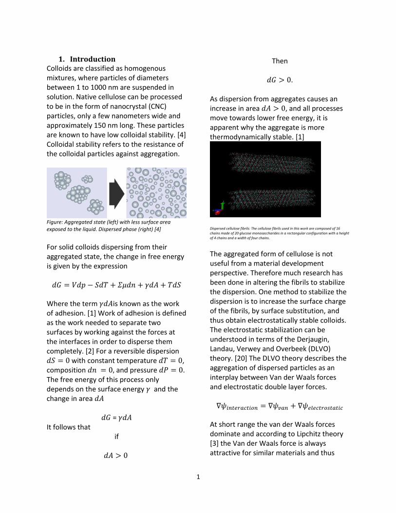
1. Introduction Colloids are classified as homogenous mixtures, where particles of diameters between 1 to 1000 nm are suspended in solution. Native cellulose can be processed to be in the form of nanocrystal (CNC) particles, only a few nanometers wide and approximately 150 nm long. These particles are known to have low colloidal stability. [4] Colloidal stability refers to the resistance of the colloidal particles against aggregation.
Figure: Aggregated state (left) with less surface area exposed to the liquid. Dispersed phase (right) [4]
For solid colloids dispersing from their aggregated state, the change in free energy is given by the expression 𝑑𝐺 = 𝑉𝑑𝑝 − 𝑆𝑑𝑇 + 𝛴𝜇𝑑𝑛 + 𝛾𝑑𝐴 + 𝑇𝑑𝑆
Where the term 𝛾𝑑𝐴is known as the work of adhesion. [1] Work of adhesion is defined as the work needed to separate two surfaces by working against the forces at the interfaces in order to disperse them completely. [2] For a reversible dispersion 𝑑𝑆 = 0 with constant temperature 𝑑𝑇 = 0, composition 𝑑𝑛 = 0, and pressure 𝑑𝑃 = 0. The free energy of this process only depends on the surface energy 𝛾 and the change in area 𝑑𝐴
𝑑𝐺 = 𝛾𝑑𝐴 It follows that
if
𝑑𝐴 > 0
Then
𝑑𝐺 > 0.
As dispersion from aggregates causes an increase in area 𝑑𝐴 > 0, and all processes move towards lower free energy, it is apparent why the aggregate is more thermodynamically stable. [1]
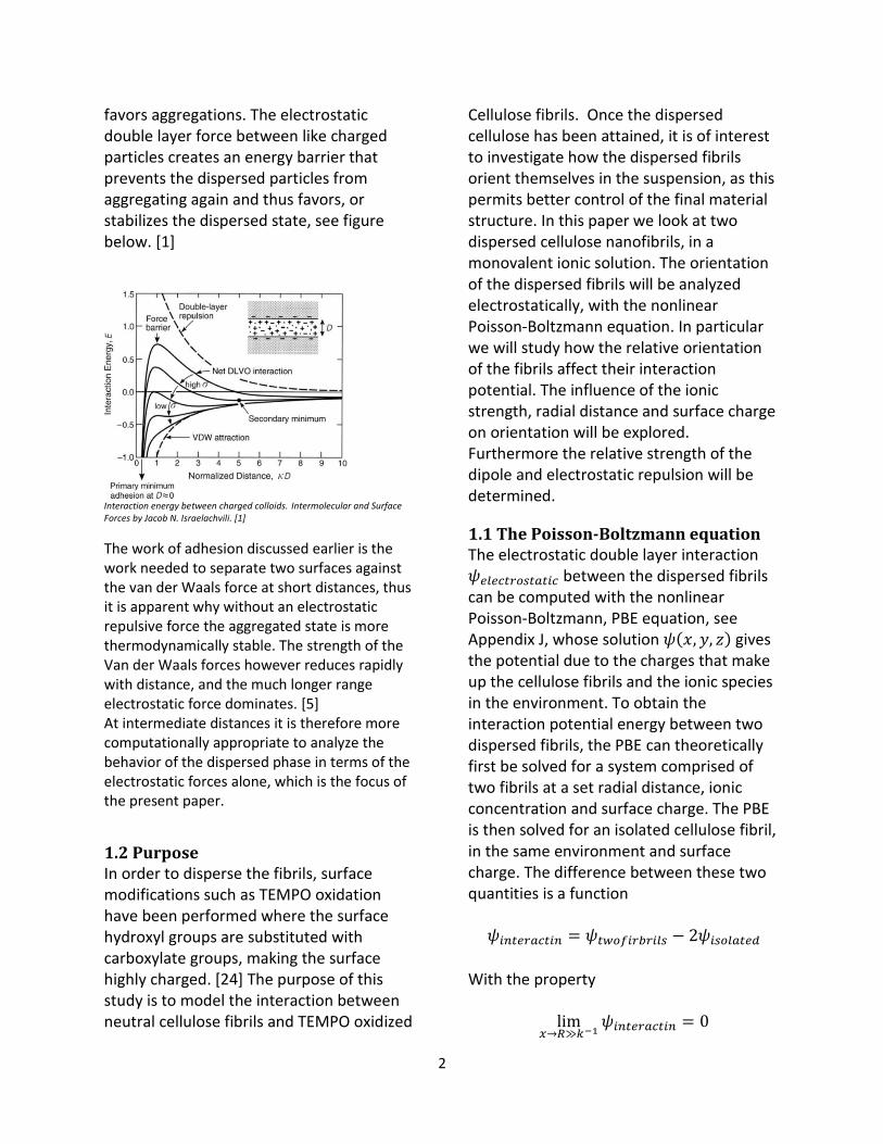
Dispersed cellulose fibrils: The cellulose fibrils used in this work are composed of 16 chains made of 20 glucose monosaccharides in a rectangular configuration with a height of 4 chains and a width of four chains.
The aggregated form of cellulose is not useful from a material development perspective. Therefore much research has been done in altering the fibrils to stabilize the dispersion. One method to stabilize the dispersion is to increase the surface charge of the fibrils, by surface substitution, and thus obtain electrostatically stable colloids. The electrostatic stabilization can be understood in terms of the Derjaugin, Landau, Verwey and Overbeek (DLVO) theory. [20] The DLVO theory describes the aggregation of dispersed particles as an interplay between Van der Waals forces and electrostatic double layer forces. ∇𝜓𝑖𝑛𝑡𝑒𝑟𝑎𝑐𝑡𝑖𝑜𝑛 = ∇𝜓𝑣𝑎𝑛 + ∇𝜓𝑒𝑙𝑒𝑐𝑡𝑟𝑜𝑠𝑡𝑎𝑡𝑖𝑐
At short range the van der Waals forces dominate and according to Lipchitz theory [3] the Van der Waals force is always attractive for similar materials and thus
2
favors aggregations. The electrostatic double layer force between like charged particles creates an energy barrier that prevents the dispersed particles from aggregating again and thus favors, or stabilizes the dispersed state, see figure below. [1]
Interaction energy between charged colloids. Intermolecular and Surface Forces by Jacob N. Israelachvili. [1]
The work of adhesion discussed earlier is the work needed to separate two surfaces against the van der Waals force at short distances, thus it is apparent why without an electrostatic repulsive force the aggregated state is more thermodynamically stable. The strength of the Van der Waals forces however reduces rapidly with distance, and the much longer range electrostatic force dominates. [5] At intermediate distances it is therefore more computationally appropriate to analyze the behavior of the dispersed phase in terms of the electrostatic forces alone, which is the focus of the present paper.
1.2 Purpose In order to disperse the fibrils, surface modifications such as TEMPO oxidation have been performed where the surface hydroxyl groups are substituted with carboxylate groups, making the surface highly charged. [24] The purpose of this study is to model the interaction between neutral cellulose fibrils and TEMPO oxidized
Cellulose fibrils. Once the dispersed cellulose has been attained, it is of interest to investigate how the dispersed fibrils orient themselves in the suspension, as this permits better control of the final material structure. In this paper we look at two dispersed cellulose nanofibrils, in a monovalent ionic solution. The orientation of the dispersed fibrils will be analyzed electrostatically, with the nonlinear Poisson-Boltzmann equation. In particular we will study how the relative orientation of the fibrils affect their interaction potential. The influence of the ionic strength, radial distance and surface charge on orientation will be explored. Furthermore the relative strength of the dipole and electrostatic repulsion will be determined.
1.1 The Poisson-Boltzmann equation The electrostatic double layer interaction 𝜓𝑒𝑙𝑒𝑐𝑡𝑟𝑜𝑠𝑡𝑎𝑡𝑖𝑐 between the dispersed fibrils can be computed with the nonlinear Poisson-Boltzmann, PBE equation, see Appendix J, whose solution 𝜓(𝑥, 𝑦, 𝑧) gives the potential due to the charges that make up the cellulose fibrils and the ionic species in the environment. To obtain the interaction potential energy between two dispersed fibrils, the PBE can theoretically first be solved for a system comprised of two fibrils at a set radial distance, ionic concentration and surface charge. The PBE is then solved for an isolated cellulose fibril, in the same environment and surface charge. The difference between these two quantities is a function 𝜓𝑖𝑛𝑡𝑒𝑟𝑎𝑐𝑡𝑖𝑛 = 𝜓𝑡𝑤𝑜𝑓𝑖𝑟𝑏𝑟𝑖𝑙𝑠 − 2𝜓𝑖𝑠𝑜𝑙𝑎𝑡𝑒𝑑
With the property
lim𝑥→𝑅≫𝑘−1
𝜓𝑖𝑛𝑡𝑒𝑟𝑎𝑐𝑡𝑖𝑛 = 0
3
Where x is the distance between the colloids
R is some finite distance much larger than the Debye length 𝜅−1
and is known as the electrostatic interaction potential 𝜓𝑒𝑙𝑒𝑐𝑡𝑟𝑜𝑠𝑡𝑎𝑡𝑖𝑐. By comparing the 𝜓𝑒𝑙𝑒𝑐𝑡𝑟𝑜𝑠𝑡𝑎𝑡𝑖𝑐 for different orientations, the naturally adopted orientation for two fibrils can determined as the net force acting on the fibrils is always directed in the direction of the negative potential gradient, and thus the direction of maximum decrease of potential energy.
�⃗� = −𝑞∇ψelectrostatic See Appendix D.
1.3 Theory - Electrostatic potential for finite rectangular fibrils Consider an isolated fibril in solution, since the surface is charged an ion-exclusion layer will form around it, whose domain will be denoted 𝛺2. The fibril itself will belong to domain 𝛺1 and the solvent will be 𝛺3. We treat the solvent and exclusion layer as continuous medium with a certain dielectric constant, disregarding the particle features of the solvent and the ions residing in it, we model the ions as a continues charge distribution, see Appendix I-J for more information. The charge density and electric potential is related by the Poisson equation. To obtain the potential distribution around the fibril, we apply Poisson equation to every region separately. That is, for 𝛺𝑘
𝛻2𝜓(𝑟)𝑘 = −𝜌(𝑟)𝑘
𝜖𝑘
Region 𝜴𝟏- The dispersed fibril As we do not model electrons, we assign
every particle making up the fibril, a partial charge. In domain 𝛺1 the potential made by these partial charges is given by the expression:
𝜓1(𝑟) = ∑𝑞𝑖4𝜋𝜖1
1
|𝑟 − 𝑟𝑖|
𝑛
𝑖=1
Which is simply the Columbic potential. Where 𝑟𝑖 is the position of the i:th charge, and n is the total number of charges in region 𝛺1. Applying Green's function for the Laplacian we obtain [6].
𝛻2𝛹1(𝑟) =∑−4𝜋𝑞𝑖𝜖1
𝛿(𝑟 − 𝑟𝑖)
𝑛
𝑖=1
where
𝛿 𝑖𝑠 𝑡ℎ𝑒 𝑑𝑖𝑟𝑎𝑐 𝑑𝑒𝑙𝑡𝑎 𝑓𝑢𝑛𝑐𝑡𝑖𝑜𝑛
𝛿(𝑟 − 𝑟𝑖) = {∞ 𝑓𝑜𝑟 𝑟 = 𝑟𝑖0 𝑓𝑜𝑟 𝑟 ≠ 𝑟𝑖
Region 𝜴𝟐- Ion exclusion layer In the ion exclusion layer there are no charges, therefore by gauss's law, see Appendix C.
∇𝜓22 = 0
Region 𝜴𝟑- Solvent The concentration at any point (𝑥, 𝑦, 𝑧) depends on the energy needed to bring all the ions there as discussed in Appendix J, and thus the charge density is in general given by the expression
𝜌(𝑥, 𝑦, 𝑧) = 𝑒(∑𝑐0𝑖𝑒−𝜓(𝑥,𝑦,𝑧) 𝑞𝑖𝑒/𝑘𝑏𝑇
𝑁
𝑖=1
−∑𝑐0𝑗𝑒𝜓(𝑥,𝑦,𝑧) 𝑞𝑗𝑒/𝑘𝑏𝑇)
𝑀
𝑗=1
Where 𝜌 is the charge density e is the electron charge
𝑐0 is the bulk concentration of the free ions
4
𝜓 is the electrostatic potential 𝑞𝑖is the valence
𝑘𝐵 is the Boltzmann constant T is the absolute temperature
Assuming there is only one variety of positive and negative ions in the solution and that the bulk concentration of both are equal (𝑐0− = 𝑐0+) the summation may be dropped and we obtain the expression
𝜌(𝑥, 𝑦, 𝑧) = 𝑒(𝑐0𝑒−𝜓(𝑥,𝑦,𝑧) 𝑒𝑞
𝑘𝑏𝑇 − 𝑐0𝑒𝜓(𝑥,𝑦,𝑧)𝑒 𝑞
𝑘𝑏𝑇 )
Noting that the hyperbolic function of sine is
𝑠𝑖𝑛ℎ(𝑥) =𝑒𝑥 − 𝑒−𝑥
2
and so the potential due to the ionic distribution is given by the expression
𝛻2𝜓(𝑥, 𝑦, 𝑧) =2𝑒𝑐0𝜖3
𝑠𝑖𝑛ℎ (𝜓(𝑥, 𝑦, 𝑧) 𝑞𝑖
𝑘𝐵𝑇)
To get an expression for the combined regions we introduce two functions
𝜖(𝑥, 𝑦, 𝑧) = {𝜖1 𝑖𝑓 𝑟 ∈ Ω1
𝜖2 = 𝜖3 𝑖𝑓 𝑟 ∈ Ω2 𝑜𝑟 𝑟 ∈ Ω3
𝜅(𝑥, 𝑦, 𝑧) = {0 𝑖𝑓 𝑟 ∈ Ω1 𝑜𝑟 𝑟 ∈ Ω2
√𝜖3𝑘 𝑖𝑓 𝑟 ∈ Ω3
Furthermore to ensure that the solution 𝜓(𝑥, 𝑦, 𝑧) is continues on the boundary regions between Ω1, Ω2 and Ω3 we require that the function takes the same value on the boundary [6]
𝜓𝑘(𝑥, 𝑦, 𝑧) = 𝜓𝑘+1(𝑥, 𝑦, 𝑧)
Boundary’s Elliptic partial differential equations, are time independent, and thus describe steady
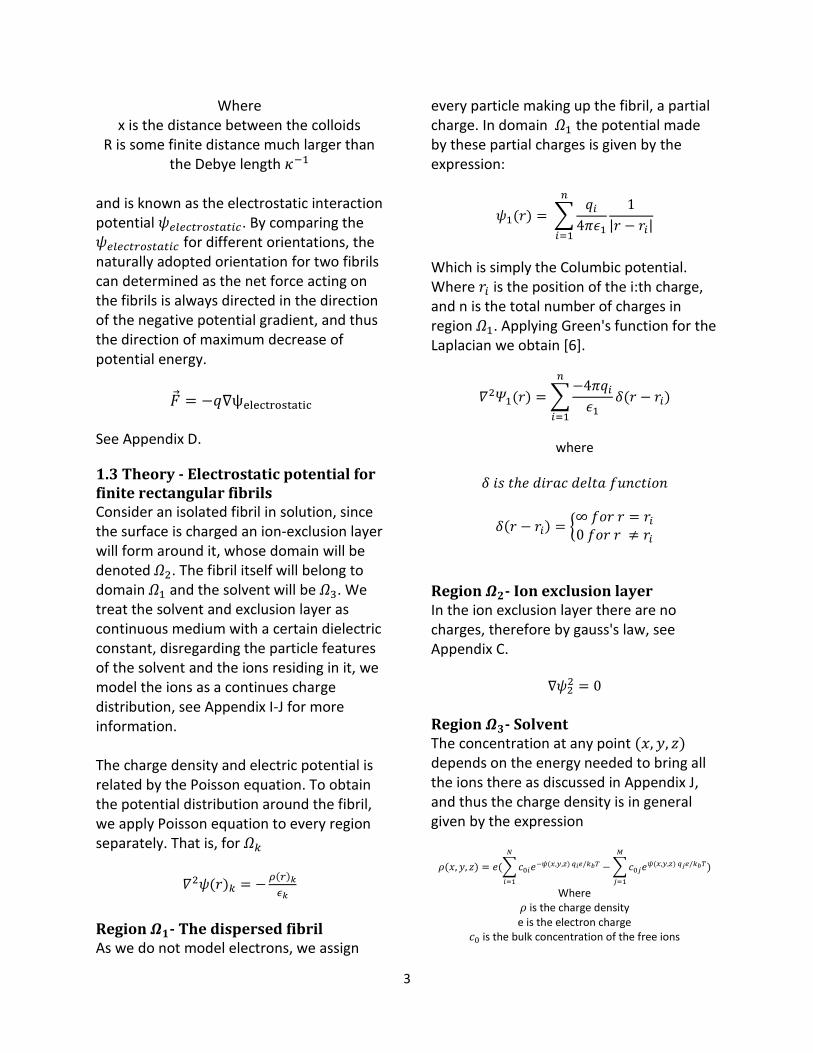
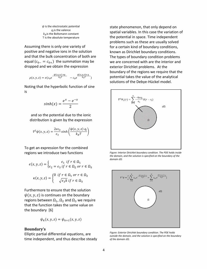
state phenomenon, that only depend on spatial variables. In this case the variation of the potential in space. Time independent problems such as these are usually solved for a certain kind of boundary conditions, known as Dirichlet boundary conditions. The types of boundary condition problems we are concerned with are the interior and exterior Dirichlet problems. At the boundary of the regions we require that the potential takes the value of the analytical solutions of the Debye-Hückel model.
Figure: Interior Dirichlet boundary condition. The PDE holds inside the domain, and the solution is specified on the boundary of the domain 𝑑Ω
Figure: Exterior Dirichlet boundary condition. The PDE holds outside the domain, and the solution is specified on the boundary of the domain 𝑑Ω
5
𝜓(𝑥, 𝑦, 𝑧) = 𝜓(𝑥, 𝑦, 𝑧)𝐷𝑒𝑏𝑦𝑒−Hückel
For (𝑥, 𝑦, 𝑧) ∈ 𝑑Ω
Then the full nonlinear Poisson-Boltzmann equation takes the form
−𝛻(𝜖(𝑥, 𝑦, 𝑧)𝛻𝜓(𝑥, 𝑦, 𝑧)) + 𝜅2 (𝑘𝐵𝑇
𝑧𝑒) 𝑠𝑖𝑛ℎ (
𝑞𝑖𝑒𝜓(𝑥, 𝑦, 𝑧)
𝑘𝐵𝑇)
= 4𝜋∑𝑞𝑖𝛿((𝑥, 𝑦, 𝑧) − (𝑥𝑖,𝑦𝑖,𝑧𝑖))
𝑛
𝑖=1
Where
𝜓 is the electrostatic potential 𝜅 𝑖𝑠 𝑡ℎ𝑒 𝑖𝑛𝑣𝑒𝑟𝑠𝑒 𝐷𝑒𝑏𝑦𝑒 𝑙𝑒𝑛𝑔𝑡ℎ 𝑓𝑢𝑛𝑐𝑡𝑖𝑜𝑛 𝑑𝑒𝑓𝑖𝑒𝑛𝑑 𝑎𝑏𝑜𝑣𝑒.
𝑞𝑖 is the valiancy of the ions 𝑘𝐵is the Boltzmann constant
𝑇 is the absolute temperature in kelvin 𝜖 is the dielectric constant function defined above
𝑒 is the electron charge
2. Method In this project the interaction potential energy was modeled using computer simulations. The software package APBS solves the nonlinear Poisson-Boltzmann equation numerically with the finite element method as is described in detail in the paper: The Poisson-Boltzmann Equation, Analysis and Multilevel Numerical Solution, M. J. Holst. [6] The exact procedure and settings used are outlined in Appendix P.
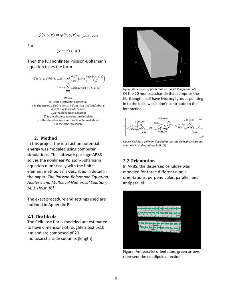
2.1 The fibrils The Cellulose fibrils modeled are estimated to have dimensions of roughly 2.5x2.5x10 nm and are composed of 20 monosaccharaide subunits (length).
Figure: Dimensions of fibrils that we model. Rough estimate.
Of the 20 monosaccharide that comprise the fibril length, half have hydroxyl groups pointing in to the bulk, which don’t contribute to the interaction.
Figure: Cellulose polymer illustrating that the O6 hydroxyl groups alternate in and out of the bulk. [2]
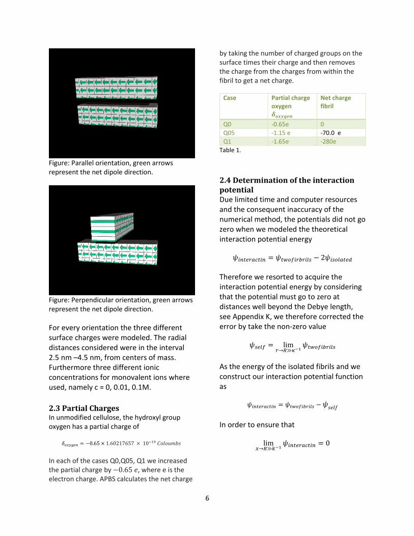
2.2 Orientation In APBS, the dispersed cellulose was modeled for three different dipole orientations: perpendicular, parallel, and antiparallel.
Figure: Antiparallel orientation, green arrows represent the net dipole direction.
6
Figure: Parallel orientation, green arrows represent the net dipole direction.
Figure: Perpendicular orientation, green arrows represent the net dipole direction.
For every orientation the three different surface charges were modeled. The radial distances considered were in the interval 2.5 nm –4.5 nm, from centers of mass. Furthermore three different ionic concentrations for monovalent ions where used, namely c = 0, 0.01, 0.1M.
2.3 Partial Charges In unmodified cellulose, the hydroxyl group oxygen has a partial charge of
𝛿𝑜𝑥𝑦𝑔𝑒𝑛 = −0.65 × 1.60217657 × 10−19 𝐶𝑜𝑙𝑜𝑢𝑚𝑏𝑠
In each of the cases Q0,Q05, Q1 we increased the partial charge by −0.65 𝑒, where e is the electron charge. APBS calculates the net charge
by taking the number of charged groups on the surface times their charge and then removes the charge from the charges from within the fibril to get a net charge.
Case Partial charge oxygen 𝜹𝒐𝒙𝒚𝒈𝒆𝒏
Net charge fibril
Q0 -0.65e 0
Q05 -1.15 e -70.0 e
Q1 -1.65e -280e
Table 1.
2.4 Determination of the interaction potential Due limited time and computer resources and the consequent inaccuracy of the numerical method, the potentials did not go zero when we modeled the theoretical interaction potential energy
𝜓𝑖𝑛𝑡𝑒𝑟𝑎𝑐𝑡𝑖𝑛 = 𝜓𝑡𝑤𝑜𝑓𝑖𝑟𝑏𝑟𝑖𝑙𝑠 − 2𝜓𝑖𝑠𝑜𝑙𝑎𝑡𝑒𝑑
Therefore we resorted to acquire the interaction potential energy by considering that the potential must go to zero at distances well beyond the Debye length, see Appendix K, we therefore corrected the error by take the non-zero value
𝜓𝑠𝑒𝑙𝑓 = lim𝑟→𝑅≫𝜅−1
𝜓𝑡𝑤𝑜𝑓𝑖𝑏𝑟𝑖𝑙𝑠
As the energy of the isolated fibrils and we construct our interaction potential function as
𝜓𝑖𝑛𝑡𝑒𝑟𝑎𝑐𝑡𝑖𝑛 = 𝜓𝑡𝑤𝑜𝑓𝑖𝑏𝑟𝑖𝑙𝑠 −𝜓𝑠𝑒𝑙𝑓
In order to ensure that
lim𝑥→𝑅≫𝑘−1
𝜓𝑖𝑛𝑡𝑒𝑟𝑎𝑐𝑡𝑖𝑛 = 0
7
2.5 The Poisson-Boltzmann equation Since there was fluctuations in the data, we fit the data to a function of the form
𝑓 = 𝛼𝑒−𝑘𝑥
As this is predicted to be the form of the potential drop by DLVO theory based on the Poisson-Boltzmann equation for the interaction potential between two surfaces.
𝜓 =64𝑐0𝑘𝐵𝑇
𝜅tanh (
𝜓0𝑞
4𝑘𝐵𝑇) 𝑒−𝜅𝑥
2.6 The Poisson equation When there are no free ions in the solution, the Poisson-Boltzmann equation turns to the Poisson equation, which as was shown in appendix F predicts a linear potential drop, for these cases we fit to a linear polynomial of the form
𝑓 = 𝑎𝑥 + 𝑏
2.7 Additional remarks The data from APBS is calculated with the distance taken from the center of mass of both fibrils. With respect to their centers of mass, they are never closer than 2.5 nm. In the DLVO theory, one considerers instead the radial distance from surface to surface. In order to correct for this in our model, we translated the curves.
𝑟𝑟 = 𝑟𝑐𝑒𝑛𝑡𝑒𝑟 − 2𝛿
Where 𝑟𝑠 is the distance between the surfaces and 𝛿 is the distance from the center of mass of each fibril to it’s own surface.
8
3. Results and Discussion The method showed fundamental problems with calculating the potential energy. Firstly there was the issue of the potential function coming out from APBS not abiding to the criteria
lim𝑥→𝑅≫𝑘−1
𝜓𝑖𝑛𝑡𝑒𝑟𝑎𝑐𝑡𝑖𝑛 = 0
Meaning that the potential energy predicted by APBS was converging to a finite, yet none zero value for distances well beyond where the interaction should sensibly go to zero. By taking the non-zero value
lim𝑥→𝑅≫𝑘−1
𝜓𝑖𝑛𝑡𝑒𝑟𝑎𝑐𝑡𝑖𝑛 = 𝐾
As the self-energy of the fibrils, and then manipulating the data from APBS such that it goes to zero was not possible in a satisfactory manner for all cases. Besides correcting so that the potential goes to zero, we also needed to make sure that the Debye lengths were correct after the translation.
3.1 Debye length In appendix K, we showed that the Debye length is given by the expression
𝜅−1 =1
√2𝑐𝑖
0𝑒2
𝜖𝜖0𝑘𝐵𝑇
Based on this we computed the Debye lengths independently of APBS for the 0.1M and 0.01M cases.
𝜅−1
=1
√2 × 0.01 × 103 × 6.022 × 1022 × (1.6 × 10−19)2
78 × 8.85 × 10−12 × 1.38 × 10−23 × 298
𝜅−1 = 3.03 𝑛𝑚
𝜅−1
=1
√2 × 0.1 × 103 × 6.022 × 1023 × (1.6 × 10−19)2
78 × 8.85 × 10−12 × 1.38 × 10−23 × 298
𝜅−1 = 0.95 𝑛𝑚
Concentration Debye length
0.01M 3.03 𝑛𝑚 0.1 M 0.95 𝑛𝑚
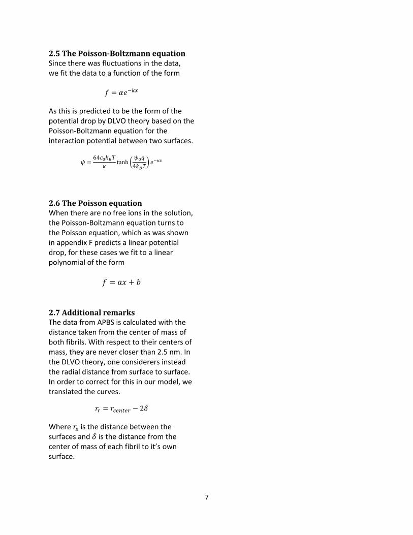
Table A The Debye length for the 0.1M case was 0.9 nm and for a 0.01M solution 3nm. Meaning that the interaction potential energies should go to zero at around 6 nm and 16 nm respectively see figure A below, for further discussion see Appendix L.
Figure A: Interaction potential per unit area 𝜓 =
64𝑐0𝑘𝐵𝑇
𝜅tanh (
𝜓0𝑞
4𝑘𝐵𝑇) 𝑒−𝜅𝑥
for two surfaces in a monovalent symmetric salt solution, with concentrations 𝑐 = 0.1𝑀 (top figure) and 𝑐 = 0.01𝑀 (bottom figure). Illustrates that the Debye length is independent of surface potential and shows the characteristic interaction lengths.
Thus correcting the Debye lengths proved to be an impossible task with 298x298x298 grid points for the finite element method, as can be seen in figure 1,2 and 4.
9
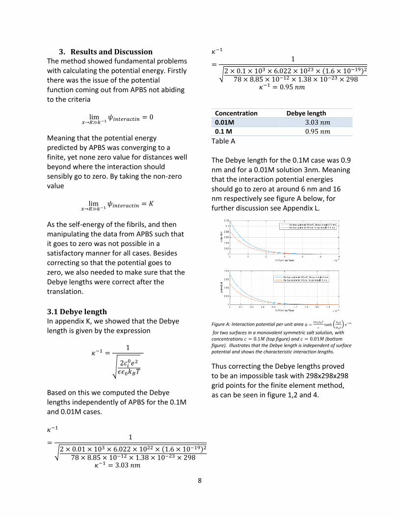
Figure 1: Effect of charge on interaction potential for antiparallel fibrils. Data values fitted to the DLVO anticipated curve. 298x298x298 grid points for the finite element method
The fact that the Q0, antiparallel case in figure 1, does not match the electrostatic interaction potential predicted by DLVO theory, is however not surprising, as the Poisson-Boltzmann equation is a partial differential equation relating the interaction potential between charged particles. It is however surprising that the interaction potential for the Q0 surface fluctuates quite a bite around zero. This is hypothesized to be due to numerical error. It thus serves as a good indicator for the overall inaccuracy in all the calculations.
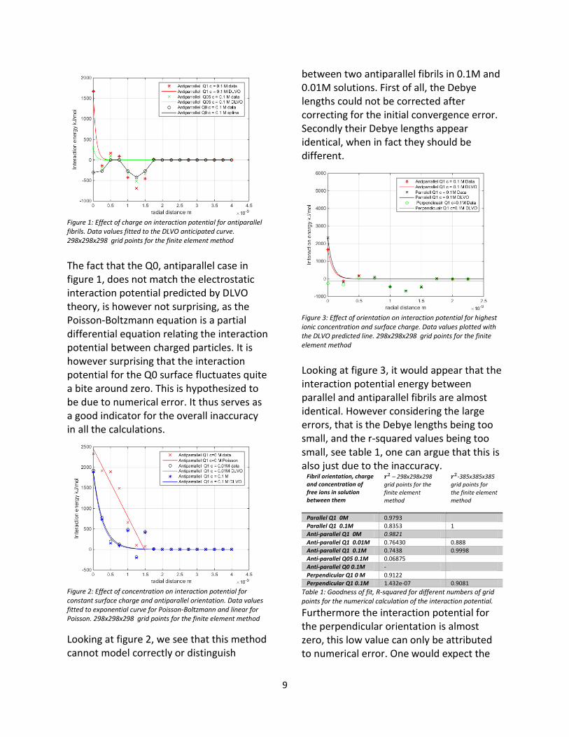
Figure 2: Effect of concentration on interaction potential for constant surface charge and antiparallel orientation. Data values fitted to exponential curve for Poisson-Boltzmann and linear for Poisson. 298x298x298 grid points for the finite element method
Looking at figure 2, we see that this method cannot model correctly or distinguish
between two antiparallel fibrils in 0.1M and 0.01M solutions. First of all, the Debye lengths could not be corrected after correcting for the initial convergence error. Secondly their Debye lengths appear identical, when in fact they should be different.
Figure 3: Effect of orientation on interaction potential for highest ionic concentration and surface charge. Data values plotted with the DLVO predicted line. 298x298x298 grid points for the finite element method
Looking at figure 3, it would appear that the interaction potential energy between parallel and antiparallel fibrils are almost identical. However considering the large errors, that is the Debye lengths being too small, and the r-squared values being too small, see table 1, one can argue that this is also just due to the inaccuracy.
Fibril orientation, charge and concentration of free ions in solution between them
𝒓𝟐 – 298x298x298 grid points for the finite element method
𝒓𝟐-385x385x385 grid points for the finite element method
Parallel Q1 0M 0.9793
Parallel Q1 0.1M 0.8353 1
Anti-parallel Q1 0M 0.9821
Anti-parallel Q1 0.01M 0.76430 0.888
Anti-parallel Q1 0.1M 0.7438 0.9998
Anti-parallel Q05 0.1M 0.06875
Anti-parallel Q0 0.1M -
Perpendicular Q1 0 M 0.9122
Perpendicular Q1 0.1M 1.432e-07 0.9081
Table 1: Goodness of fit, R-squared for different numbers of grid points for the numerical calculation of the interaction potential.
Furthermore the interaction potential for the perpendicular orientation is almost zero, this low value can only be attributed to numerical error. One would expect the
10
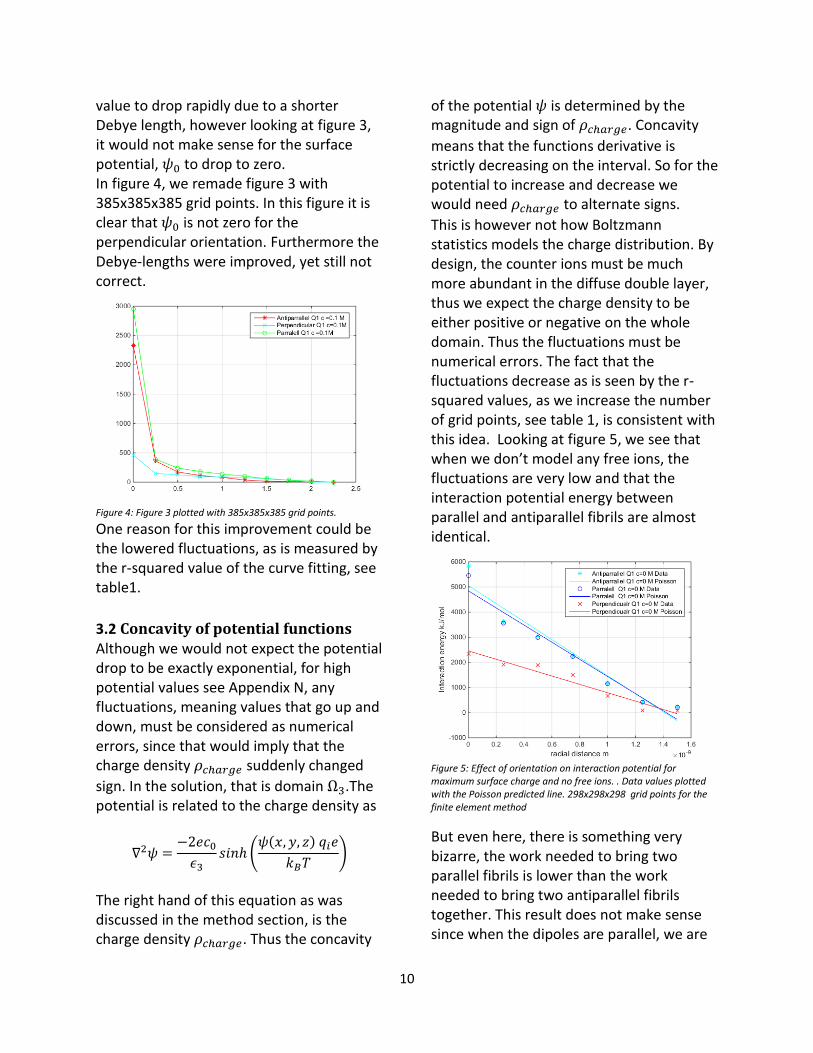
value to drop rapidly due to a shorter Debye length, however looking at figure 3, it would not make sense for the surface potential, 𝜓0 to drop to zero. In figure 4, we remade figure 3 with 385x385x385 grid points. In this figure it is clear that 𝜓0 is not zero for the perpendicular orientation. Furthermore the Debye-lengths were improved, yet still not correct.
Figure 4: Figure 3 plotted with 385x385x385 grid points.
One reason for this improvement could be the lowered fluctuations, as is measured by the r-squared value of the curve fitting, see table1.
3.2 Concavity of potential functions Although we would not expect the potential drop to be exactly exponential, for high potential values see Appendix N, any fluctuations, meaning values that go up and down, must be considered as numerical errors, since that would imply that the charge density 𝜌𝑐ℎ𝑎𝑟𝑔𝑒 suddenly changed
sign. In the solution, that is domain Ω3.The potential is related to the charge density as
∇2𝜓 =−2𝑒𝑐0𝜖3
𝑠𝑖𝑛ℎ (𝜓(𝑥, 𝑦, 𝑧) 𝑞𝑖𝑒
𝑘𝐵𝑇)
The right hand of this equation as was discussed in the method section, is the charge density 𝜌𝑐ℎ𝑎𝑟𝑔𝑒. Thus the concavity
of the potential 𝜓 is determined by the magnitude and sign of 𝜌𝑐ℎ𝑎𝑟𝑔𝑒. Concavity
means that the functions derivative is strictly decreasing on the interval. So for the potential to increase and decrease we would need 𝜌𝑐ℎ𝑎𝑟𝑔𝑒 to alternate signs.
This is however not how Boltzmann statistics models the charge distribution. By design, the counter ions must be much more abundant in the diffuse double layer, thus we expect the charge density to be either positive or negative on the whole domain. Thus the fluctuations must be numerical errors. The fact that the fluctuations decrease as is seen by the r-squared values, as we increase the number of grid points, see table 1, is consistent with this idea. Looking at figure 5, we see that when we don’t model any free ions, the fluctuations are very low and that the interaction potential energy between parallel and antiparallel fibrils are almost identical.
Figure 5: Effect of orientation on interaction potential for maximum surface charge and no free ions. . Data values plotted with the Poisson predicted line. 298x298x298 grid points for the finite element method
But even here, there is something very bizarre, the work needed to bring two parallel fibrils is lower than the work needed to bring two antiparallel fibrils together. This result does not make sense since when the dipoles are parallel, we are
11
bringing like partial charges together, which is always more energy consuming than brining two opposite partial charges together as in the case of the anti-parallel. In figure 3 and 5 this is not the case. Based on figure 5, we make the claim that the dipole interactions seam negligible, since even though the starting behavior is bizarre, the values overlap for all subsequent radial distances. Regardless of the free ion concentration or surface charge (with exception for no surface charge), the perpendicular orientation always has least potential energy. This makes sense, since the electrostatic interaction is minimized when they orient themselves perpendicularly, and so less work needs to be done in order to create system.
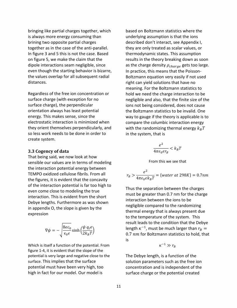
3.3 Cogency of data That being said, we now look at how sensible our values are in terms of modeling the interaction potential energy between TEMPO oxidized cellulose fibrils. From all the figures, it is evident that the concavity of the interaction potential is far too high to even come close to modeling the true interaction. This is evident from the short Debye lengths. Furthermore as was shown in appendix O, the slope is given by the expression
∇𝜓 = −√8𝑒𝑐0ϵ0𝜖
sinh (𝜓 𝑞𝑖𝑒
2𝑘𝐵𝑇)
Which is itself a function of the potential. From figure 1-4, it is evident that the slope of the potential is very large and negative close to the
surface. This implies that the surface potential must have been very high, too high in fact for our model. Our model is
based on Boltzmann statistics where the underlying assumption is that the ions described don’t interact, see Appendix I, they are only treated as scalar values, or thermodynamic states. This assumption results in the theory breaking down as soon as the charge density 𝜌𝑐ℎ𝑎𝑟𝑔𝑒 gets too large.
In practice, this means that the Poisson-Boltzmann equation very easily if not used right can yield solutions that have no meaning. For the Boltzmann statistics to hold we need the charge interaction to be negligible and also, that the finite size of the ions not being considered, does not cause the Boltzmann statistics to be invalid. One way to gauge if the theory is applicable is to compare the columbic interaction energy with the randomizing thermal energy 𝑘𝐵𝑇 in the system, that is
𝑒2
4𝜋𝜖0𝜖𝑟𝐵< 𝑘𝐵𝑇
From this we see that
𝑟𝐵 >𝑒2
4𝜋𝜖0𝜖𝑘𝐵𝑇= {𝑤𝑎𝑡𝑒𝑟 𝑎𝑡 298𝐾} = 0.7𝑛𝑚
Thus the separation between the charges must be greater than 0.7 nm for the charge interaction between the ions to be negligible compared to the randomizing thermal energy that is always present due to the temperature of the system. This result leads to the condition that the Debye length 𝜅−1, must be much larger than 𝑟𝐵 =0.7 𝑛𝑚 for Boltzmann statistics to hold, that is
𝜅−1 ≫ 𝑟𝐵
The Debye length, is a function of the solution parameters such as the free ion concentration and is independent of the surface charge or the potential created
12
from the surface. We calculated the Debye lengths to be 0.9 nm and 3 nm for 0.1M and 0.01M independent of APBS. Thus we see that the bulk concentration of the free ions, theoretically shouldn’t cause problems for our Boltzmann statistics in this system. However looking at the figures based on the APBS calculations we see that the Debye lengths, are not what they should be, and this problem is due to the potential dropping to steeply, or the concavity of the function being too high. This implies that the surface potential is too high, considering that the charge density or concavity of the potential function is
proportional to sinh (𝜓(𝑥,𝑦,𝑧)𝑒 𝑞𝑖
𝑘𝐵𝑇), we see
that high surface potentials cause the charge density of counter ions that screen the electric field to become very high. To rule out numerical errors, we can use figure 5 as a reference for the potential. Since figure 5 is based on the Poisson equation
∇𝜓2 = 0 It does not rely on statistical methods and thus should be valid, even if the Poisson-Boltzmann equation is not. We see that the interaction potential energy can go up to 6 million joules/mol. This high value can be reasonable considering that we have a mole of fibrils with 40 charged groups pressed onto each other. However these high values could cause problems for the Poisson-Boltzmann equation and cause the potential to drops off very fast. To confirm if this is the case we first need to estimate the separation between the ions 𝑟𝑖𝑜𝑛 to see if they violate the condition
𝑟𝐵 > 𝑟𝑖𝑜𝑛
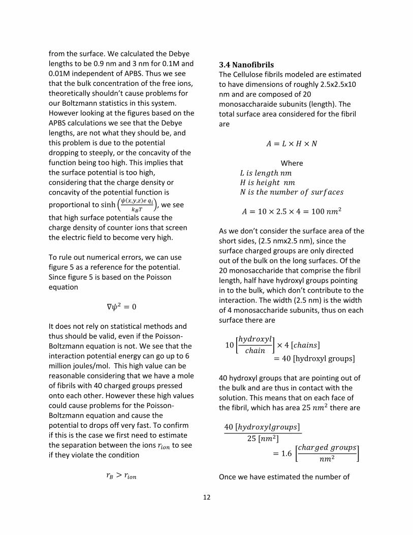
3.4 Nanofibrils The Cellulose fibrils modeled are estimated to have dimensions of roughly 2.5x2.5x10 nm and are composed of 20 monosaccharaide subunits (length). The total surface area considered for the fibril are
𝐴 = 𝐿 × 𝐻 × 𝑁
Where 𝐿 𝑖𝑠 𝑙𝑒𝑛𝑔𝑡ℎ 𝑛𝑚 𝐻 𝑖𝑠 ℎ𝑒𝑖𝑔ℎ𝑡 𝑛𝑚 𝑁 𝑖𝑠 𝑡ℎ𝑒 𝑛𝑢𝑚𝑏𝑒𝑟 𝑜𝑓 𝑠𝑢𝑟𝑓𝑎𝑐𝑒𝑠
𝐴 = 10 × 2.5 × 4 = 100 𝑛𝑚2
As we don’t consider the surface area of the short sides, (2.5 nmx2.5 nm), since the surface charged groups are only directed out of the bulk on the long surfaces. Of the 20 monosaccharide that comprise the fibril length, half have hydroxyl groups pointing in to the bulk, which don’t contribute to the interaction. The width (2.5 nm) is the width of 4 monosaccharide subunits, thus on each surface there are
10 [ℎ𝑦𝑑𝑟𝑜𝑥𝑦𝑙
𝑐ℎ𝑎𝑖𝑛] × 4 [𝑐ℎ𝑎𝑖𝑛𝑠]
= 40 [hydroxyl groups] 40 hydroxyl groups that are pointing out of the bulk and are thus in contact with the solution. This means that on each face of the fibril, which has area 25 𝑛𝑚2 there are 40 [ℎ𝑦𝑑𝑟𝑜𝑥𝑦𝑙𝑔𝑟𝑜𝑢𝑝𝑠]
25 [𝑛𝑚2]
= 1.6 [𝑐ℎ𝑎𝑟𝑔𝑒𝑑 𝑔𝑟𝑜𝑢𝑝𝑠
𝑛𝑚2]
Once we have estimated the number of
13
charged groups per unit area, we can estimate the total charge of the fibrils if we know the partial charge of each charged groups.
3.5 Surface charge density
The surface charge density 𝜎 [ 𝐶𝑜𝑙𝑜𝑢𝑚𝑏𝑠
𝑚2] is
calculated as
𝜎 =𝑄𝑛𝑒𝑡𝐴𝑟𝑒𝑎
Where 𝑄𝑛𝑒𝑡 is taken from table 1. Thus the different cases have the surface charge densities.
𝜎𝑄05 =−70× 1.60217657 × 10−19
100 × 10−18
= −0.1122 [ 𝐶𝑜𝑙𝑜𝑢𝑚𝑏𝑠
𝑚2]
𝜎𝑄1 =−280 × 1.60217657 × 10−19
100 × 10−18
= −0.4486 [𝐶𝑜𝑙𝑜𝑢𝑚𝑏𝑠
𝑚2]
Case Surface charge
𝝈 [𝑪𝒐𝒍𝒐𝒖𝒎𝒃𝒔
𝒎𝟐 ]
Q0 0
Q05 −0.1122
Q1 −0.4486
Table 2
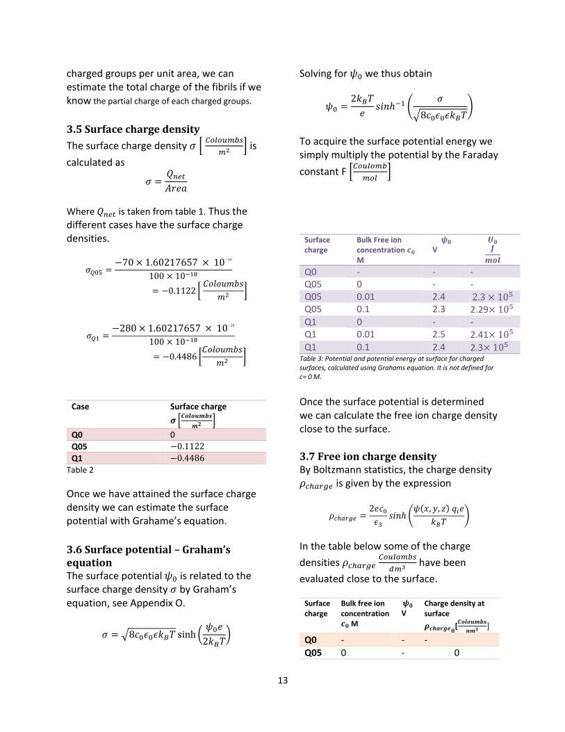
Once we have attained the surface charge density we can estimate the surface potential with Grahame’s equation.
3.6 Surface potential – Graham’s equation The surface potential 𝜓0 is related to the surface charge density 𝜎 by Graham’s equation, see Appendix O.
𝜎 = √8𝑐0𝜖0𝜖𝑘𝐵𝑇 sinh (𝜓0𝑒
2𝑘𝐵𝑇)
Solving for 𝜓0 we thus obtain
𝜓0 =2𝑘𝐵𝑇
𝑒𝑠𝑖𝑛ℎ−1 (
𝜎
√8𝑐0𝜖0𝜖𝑘𝐵𝑇)
To acquire the surface potential energy we simply multiply the potential by the Faraday
constant F [𝐶𝑜𝑢𝑙𝑜𝑚𝑏
𝑚𝑜𝑙]
Surface charge
Bulk Free ion concentration 𝒄𝟎 M
𝝍𝟎 V
𝑼𝟎 𝑱
𝒎𝒐𝒍
Q0 - - - Q05 0 - - Q05 0.01 2.4 2.3 × 10⁵ Q05 0.1 2.3 2.29× 10⁵ Q1 0 - - Q1 0.01 2.5 2.41× 10⁵ Q1 0.1 2.4 2.3× 10⁵
Table 3: Potential and potential energy at surface for charged surfaces, calculated using Grahams equation. It is not defined for c= 0 M.
Once the surface potential is determined we can calculate the free ion charge density close to the surface.
3.7 Free ion charge density By Boltzmann statistics, the charge density 𝜌𝑐ℎ𝑎𝑟𝑔𝑒 is given by the expression
𝜌𝑐ℎ𝑎𝑟𝑔𝑒 =2𝑒𝑐0𝜖3
𝑠𝑖𝑛ℎ (𝜓(𝑥, 𝑦, 𝑧) 𝑞𝑖𝑒
𝑘𝐵𝑇)
In the table below some of the charge
densities 𝜌𝑐ℎ𝑎𝑟𝑔𝑒 𝐶𝑜𝑢𝑙𝑜𝑚𝑏𝑠
𝑑𝑚3 have been
evaluated close to the surface.
Surface charge
Bulk free ion concentration 𝒄𝟎 M
𝝍𝟎 V
Charge density at surface
𝝆𝒄𝒉𝒂𝒓𝒈𝒆𝟎[𝑪𝒐𝒍𝒐𝒖𝒎𝒃𝒔
𝒏𝒎𝟑 ]
Q0 - - -
Q05 0 - 0
14
Q05 0.01 2.4 7.05 × 10¹⁵ Q05 0.1 2.3 1.43 × 10¹⁵ Q1 0 - 0
Q1 0.01 2.5 3.47 × 10¹⁷ Q1 0.1 2.4 7.05 × 10¹⁵
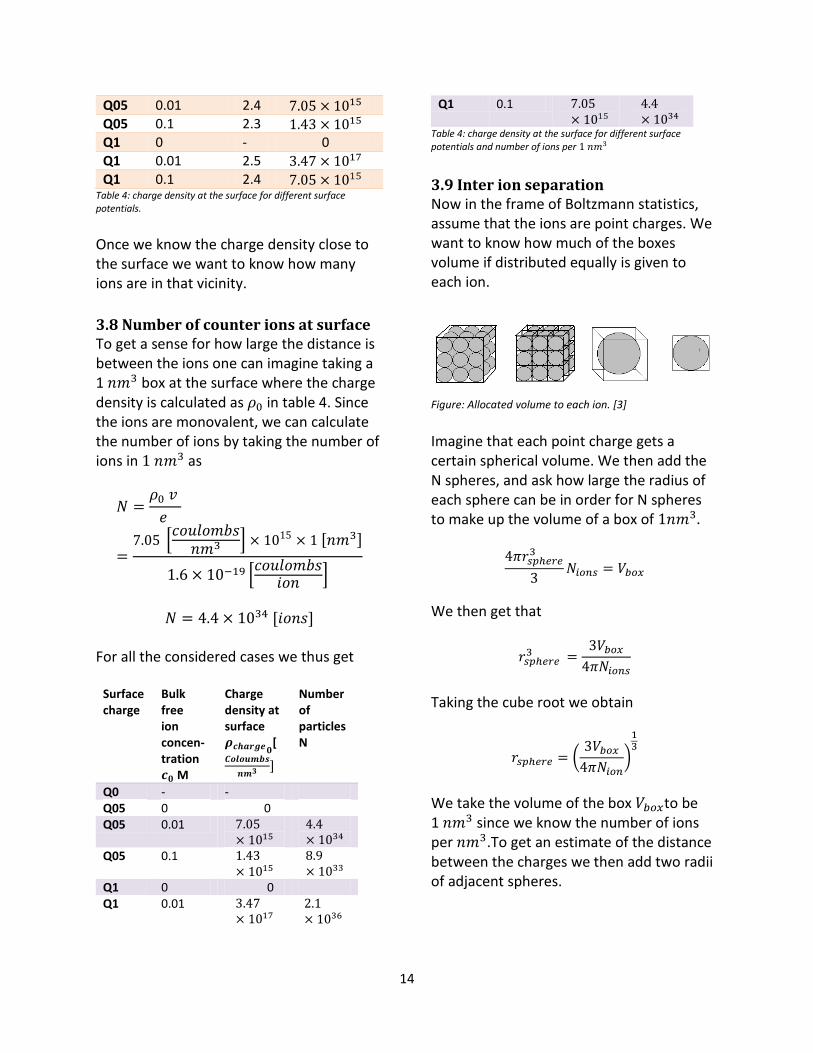
Table 4: charge density at the surface for different surface potentials. Once we know the charge density close to the surface we want to know how many ions are in that vicinity.
3.8 Number of counter ions at surface To get a sense for how large the distance is between the ions one can imagine taking a 1 𝑛𝑚3 box at the surface where the charge density is calculated as 𝜌0 in table 4. Since the ions are monovalent, we can calculate the number of ions by taking the number of ions in 1 𝑛𝑚3 as
𝑁 =𝜌0 𝑣
𝑒
=7.05 [
𝑐𝑜𝑢𝑙𝑜𝑚𝑏𝑠𝑛𝑚3 ] × 1015 × 1 [𝑛𝑚3]
1.6 × 10⁻¹⁹ [𝑐𝑜𝑢𝑙𝑜𝑚𝑏𝑠
𝑖𝑜𝑛 ]
𝑁 = 4.4 × 1034 [𝑖𝑜𝑛𝑠]
For all the considered cases we thus get
Surface charge
Bulk free ion concen-tration 𝒄𝟎 M
Charge density at surface 𝝆𝒄𝒉𝒂𝒓𝒈𝒆𝟎
[ 𝑪𝒐𝒍𝒐𝒖𝒎𝒃𝒔
𝒏𝒎𝟑 ]
Number of particles N
Q0 - - Q05 0 0 Q05 0.01 7.05
× 1015 4.4× 1034
Q05 0.1 1.43× 10¹⁵
8.9× 1033
Q1 0 0 Q1 0.01 3.47
× 1017 2.1× 1036
Q1 0.1 7.05× 10¹⁵
4.4× 1034
Table 4: charge density at the surface for different surface potentials and number of ions per 1 𝑛𝑚3
3.9 Inter ion separation Now in the frame of Boltzmann statistics, assume that the ions are point charges. We want to know how much of the boxes volume if distributed equally is given to each ion.
Figure: Allocated volume to each ion. [3]
Imagine that each point charge gets a certain spherical volume. We then add the N spheres, and ask how large the radius of each sphere can be in order for N spheres to make up the volume of a box of 1𝑛𝑚3.
4𝜋𝑟𝑠𝑝ℎ𝑒𝑟𝑒3
3𝑁𝑖𝑜𝑛𝑠 = 𝑉𝑏𝑜𝑥
We then get that
𝑟𝑠𝑝ℎ𝑒𝑟𝑒 3 =
3𝑉𝑏𝑜𝑥4𝜋𝑁𝑖𝑜𝑛𝑠
Taking the cube root we obtain
𝑟𝑠𝑝ℎ𝑒𝑟𝑒 = (3𝑉𝑏𝑜𝑥4𝜋𝑁𝑖𝑜𝑛
)
13
We take the volume of the box 𝑉𝑏𝑜𝑥to be 1 𝑛𝑚3 since we know the number of ions per 𝑛𝑚3.To get an estimate of the distance between the charges we then add two radii of adjacent spheres.
15
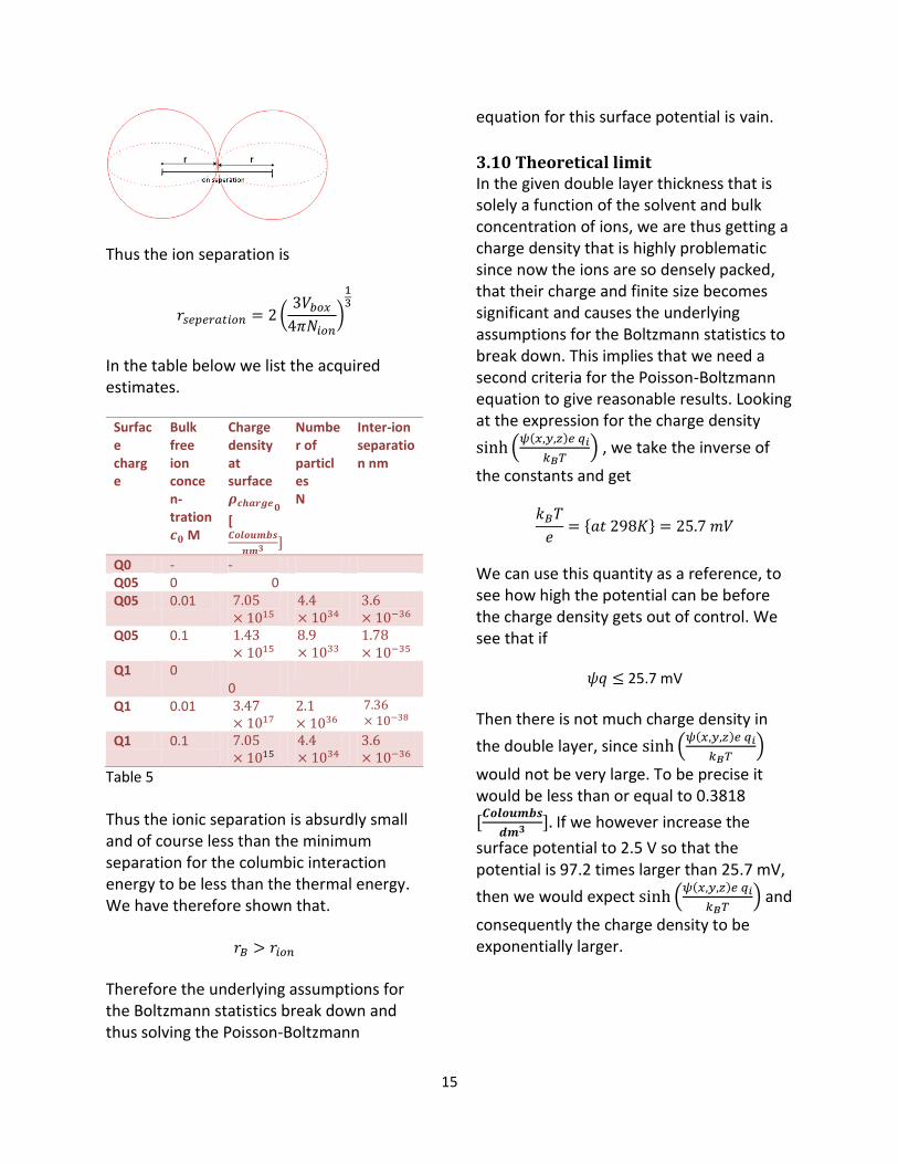
Thus the ion separation is
𝑟𝑠𝑒𝑝𝑒𝑟𝑎𝑡𝑖𝑜𝑛 = 2(3𝑉𝑏𝑜𝑥4𝜋𝑁𝑖𝑜𝑛
)
13
In the table below we list the acquired estimates.
Surface charge
Bulk free ion concen-tration 𝒄𝟎 M
Charge density at surface 𝝆𝒄𝒉𝒂𝒓𝒈𝒆𝟎[ 𝑪𝒐𝒍𝒐𝒖𝒎𝒃𝒔
𝒏𝒎𝟑 ]
Number of particles N
Inter-ion separation nm
Q0 - - Q05 0 0 Q05 0.01 7.05
× 1015 4.4× 1034
3.6× 10−36
Q05 0.1 1.43× 10¹⁵
8.9× 1033
1.78× 10⁻³⁵
Q1 0 0
Q1 0.01 3.47× 10¹⁷
2.1× 1036
7.36× 10−38
Q1 0.1 7.05× 10¹⁵
4.4× 1034
3.6× 10−36
Table 5
Thus the ionic separation is absurdly small and of course less than the minimum separation for the columbic interaction energy to be less than the thermal energy. We have therefore shown that.
𝑟𝐵 > 𝑟𝑖𝑜𝑛 Therefore the underlying assumptions for the Boltzmann statistics break down and thus solving the Poisson-Boltzmann
equation for this surface potential is vain.
3.10 Theoretical limit In the given double layer thickness that is solely a function of the solvent and bulk concentration of ions, we are thus getting a charge density that is highly problematic since now the ions are so densely packed, that their charge and finite size becomes significant and causes the underlying assumptions for the Boltzmann statistics to break down. This implies that we need a second criteria for the Poisson-Boltzmann equation to give reasonable results. Looking at the expression for the charge density
sinh (𝜓(𝑥,𝑦,𝑧)𝑒 𝑞𝑖
𝑘𝐵𝑇) , we take the inverse of
the constants and get
𝑘𝐵𝑇
𝑒= {𝑎𝑡 298𝐾} = 25.7 𝑚𝑉
We can use this quantity as a reference, to see how high the potential can be before the charge density gets out of control. We see that if
𝜓𝑞 ≤ 25.7 mV
Then there is not much charge density in
the double layer, since sinh (𝜓(𝑥,𝑦,𝑧)𝑒 𝑞𝑖
𝑘𝐵𝑇)
would not be very large. To be precise it would be less than or equal to 0.3818
[𝑪𝒐𝒍𝒐𝒖𝒎𝒃𝒔
𝒅𝒎𝟑 ]. If we however increase the
surface potential to 2.5 V so that the potential is 97.2 times larger than 25.7 mV,
then we would expect sinh (𝜓(𝑥,𝑦,𝑧)𝑒 𝑞𝑖
𝑘𝐵𝑇) and
consequently the charge density to be exponentially larger.
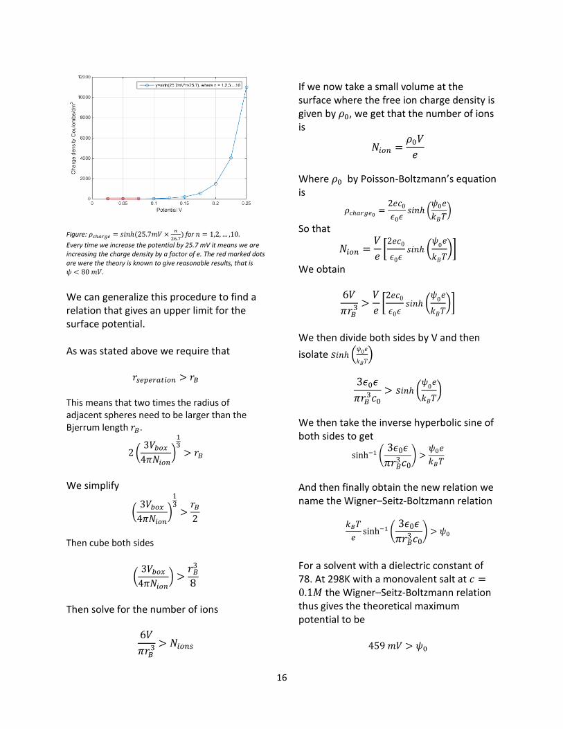
16
Figure: 𝜌𝑐ℎ𝑎𝑟𝑔𝑒 = 𝑠𝑖𝑛ℎ (25.7𝑚𝑉 ×
𝑛
26.7) for 𝑛 = 1,2,… ,10.
Every time we increase the potential by 25.7 mV it means we are increasing the charge density by a factor of e. The red marked dots are were the theory is known to give reasonable results, that is 𝜓 < 80 𝑚𝑉.
We can generalize this procedure to find a relation that gives an upper limit for the surface potential. As was stated above we require that
𝑟𝑠𝑒𝑝𝑒𝑟𝑎𝑡𝑖𝑜𝑛 > 𝑟𝐵
This means that two times the radius of adjacent spheres need to be larger than the Bjerrum length 𝑟𝐵.
2 (3𝑉𝑏𝑜𝑥4𝜋𝑁𝑖𝑜𝑛
)
13> 𝑟𝐵
We simplify
(3𝑉𝑏𝑜𝑥4𝜋𝑁𝑖𝑜𝑛
)
13>𝑟𝐵2
Then cube both sides
(3𝑉𝑏𝑜𝑥4𝜋𝑁𝑖𝑜𝑛
) >𝑟𝐵3
8
Then solve for the number of ions
6𝑉
𝜋𝑟𝐵3 > 𝑁𝑖𝑜𝑛𝑠
If we now take a small volume at the surface where the free ion charge density is given by 𝜌0, we get that the number of ions is
𝑁𝑖𝑜𝑛 =𝜌0𝑉
𝑒
Where 𝜌0 by Poisson-Boltzmann’s equation is
𝜌𝑐ℎ𝑎𝑟𝑔𝑒0 =2𝑒𝑐0𝜖0𝜖
𝑠𝑖𝑛ℎ (𝜓0𝑒
𝑘𝐵𝑇)
So that
𝑁𝑖𝑜𝑛 =𝑉
𝑒[2𝑒𝑐0
𝜖0𝜖𝑠𝑖𝑛ℎ (
𝜓0𝑒
𝑘𝐵𝑇)]
We obtain
6𝑉
𝜋𝑟𝐵3 >
𝑉
𝑒[2𝑒𝑐0
𝜖0𝜖𝑠𝑖𝑛ℎ (
𝜓0𝑒
𝑘𝐵𝑇)]
We then divide both sides by V and then
isolate 𝑠𝑖𝑛ℎ (𝜓0𝑒
𝑘𝐵𝑇)
3𝜖0𝜖
𝜋𝑟𝐵3𝑐0
> 𝑠𝑖𝑛ℎ (𝜓0𝑒
𝑘𝐵𝑇)
We then take the inverse hyperbolic sine of both sides to get
sinh−1 (3𝜖0𝜖
𝜋𝑟𝐵3𝑐0
) >𝜓0𝑒
𝑘𝐵𝑇
And then finally obtain the new relation we name the Wigner–Seitz-Boltzmann relation
𝑘𝐵𝑇
𝑒sinh−1 (
3𝜖0𝜖
𝜋𝑟𝐵3𝑐0
) > 𝜓0
For a solvent with a dielectric constant of 78. At 298K with a monovalent salt at 𝑐 =0.1𝑀 the Wigner–Seitz-Boltzmann relation thus gives the theoretical maximum potential to be
459 𝑚𝑉 > 𝜓0
17
For a monovalent free ion concentration of 𝑐 = 0.01𝑀
519 𝑚𝑉 > 𝜓0
These upper limits should however be taken with a grain of salt as it is generally accepted that the Poisson-Boltzmann equation gives reasonable results for surface potentials up to 80mV [7], this corresponds to a free ion charge density at
the surface of 3.7903 [𝑪𝒐𝒍𝒐𝒖𝒎𝒃𝒔
𝒅𝒎𝟑]. The
Wigner–Seitz-Boltzmann relation gives the maximum surface potential only in the sense that the electrostatic interaction between the ions don’t violate the Boltzmann statistics.
3.11 Conclusion In this study we have confirmed that the interaction potential energy between cellulose nanofibrils surface substituted with TEMPO oxidation cannot be modeled
with the Poisson-Boltzmann equation, as the surface potential is too high for Boltzmann statics to hold. This parts of the study is therefore inconclusive. We can however conclude that for highly charged fibrils modeled with no free ions, where we don’t rely on Boltzmann statistics and thus the Poisson equation is valid, the dipole interactions appear to be negligible in comparison to the surface charge contribution to the interaction potential. Furthermore we have combined the Bjerrum length, The Poisson-Boltzmann equation and the Wigner–Seitz radius to derive a new relation called the Wigner–Seitz-Boltzmann relation that predicts the theoretical upper limit for the surface potential for the Poisson-Boltzmann equation applied to monovalent free ionic solutions strictly in terms of bulk parameters.

18
The Poisson-Boltzmann equation
19
In the appendices below, we first discuss the concepts of charge interactions in free space, in particular the relationship between force and potential energy, and then derive the equations that extend charge interactions in solutions, with and without the presence of free ions.
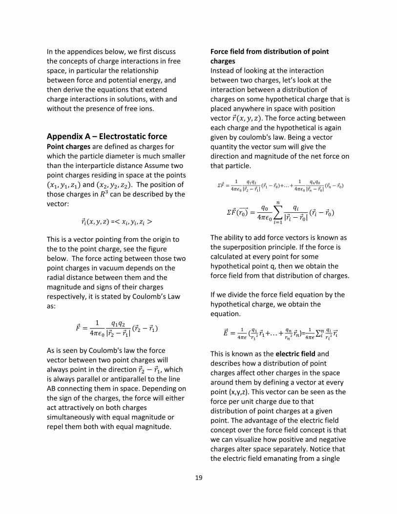
Appendix A – Electrostatic force Point charges are defined as charges for which the particle diameter is much smaller than the interparticle distance Assume two point charges residing in space at the points (𝑥1, 𝑦1, 𝑧1) and (𝑥2, 𝑦2, 𝑧2). The position of those charges in 𝑅³ can be described by the vector:
𝑟𝑖(𝑥, 𝑦, 𝑧) =< 𝑥𝑖 , 𝑦𝑖 , 𝑧𝑖 >
This is a vector pointing from the origin to the to the point charge, see the figure below. The force acting between those two point charges in vacuum depends on the radial distance between them and the magnitude and signs of their charges respectively, it is stated by Coulomb’s Law as:
�⃗� =1
4𝜋𝜖0
𝑞1𝑞2|𝑟2 − 𝑟1|
(𝑟2 − 𝑟1)
As is seen by Coulomb's law the force vector between two point charges will always point in the direction 𝑟2 − 𝑟1, which is always parallel or antiparallel to the line AB connecting them in space. Depending on the sign of the charges, the force will either act attractively on both charges simultaneously with equal magnitude or repel them both with equal magnitude.
Force field from distribution of point charges Instead of looking at the interaction between two charges, let’s look at the interaction between a distribution of charges on some hypothetical charge that is placed anywhere in space with position vector 𝑟(𝑥, 𝑦, 𝑧). The force acting between each charge and the hypothetical is again given by coulomb's law. Being a vector quantity the vector sum will give the direction and magnitude of the net force on that particle.
𝛴�⃗� =1
4𝜋𝜖0
𝑞1𝑞2|𝑟2 − 𝑟1|
(𝑟1 − 𝑟0)+. . . +1
4𝜋𝜖0
𝑞𝑛𝑞0|𝑟𝑛 − 𝑟0|
(𝑟𝑛 − 𝑟0)
𝛴�⃗�(𝑟0)⃗⃗⃗⃗⃗⃗ =𝑞04𝜋𝜖0
∑𝑞𝑖
|𝑟𝑖 − 𝑟0|(𝑟𝑖 − 𝑟0)
𝑛
𝑖=1
The ability to add force vectors is known as the superposition principle. If the force is calculated at every point for some hypothetical point q, then we obtain the force field from that distribution of charges. If we divide the force field equation by the hypothetical charge, we obtain the equation.
�⃗⃗� =1
4𝜋𝜖(𝑞1
𝑟1²𝑟1+. . . +
𝑞𝑛
𝑟𝑛²𝑟𝑛)=
1
4𝜋𝜖∑
𝑞𝑖
𝑟𝑖²𝑟𝑖⃗⃗⃗
𝑛𝑖
This is known as the electric field and describes how a distribution of point charges affect other charges in the space around them by defining a vector at every point (x,y,z). This vector can be seen as the force per unit charge due to that distribution of point charges at a given point. The advantage of the electric field concept over the force field concept is that we can visualize how positive and negative charges alter space separately. Notice that the electric field emanating from a single
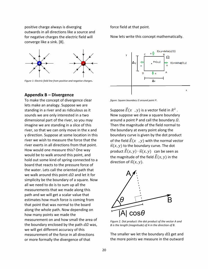
20
positive charge always is diverging outwards in all directions like a source and for negative charges the electric field will converge like a sink. [8].
Figure 1: Electric field line from positive and negative charges.
Appendix B – Divergence To make the concept of divergence clear lets make an analogy. Suppose we are standing in a river and as ridiculous as it sounds we are only interested in a two dimensional part of the river, so you may imagine we are standing in a slice of this river, so that we can only move in the x and y direction. Suppose at some location in this river we wish to measure the force that the river exerts in all directions from that point. How would one measure this? One way would be to walk around this point, and hold out some kind of spring connected to a board that reacts to the pressure force of the water. Lets call the oriented path that we walk around this point 𝑑𝛺 and let it for simplicity be the boundary of a square. Now all we need to do is to sum up all the measurements that we made along this path and we will get a scalar value that estimates how much force is coming from that point that was normal to the board along the whole path. Now depending on how many points we made the measurement on and how small the area of the boundary enclosed by the path 𝑑𝛺 was, we will get different accuracy of this measurement of the force in all directions or more formally the divergence of that
force field at that point.
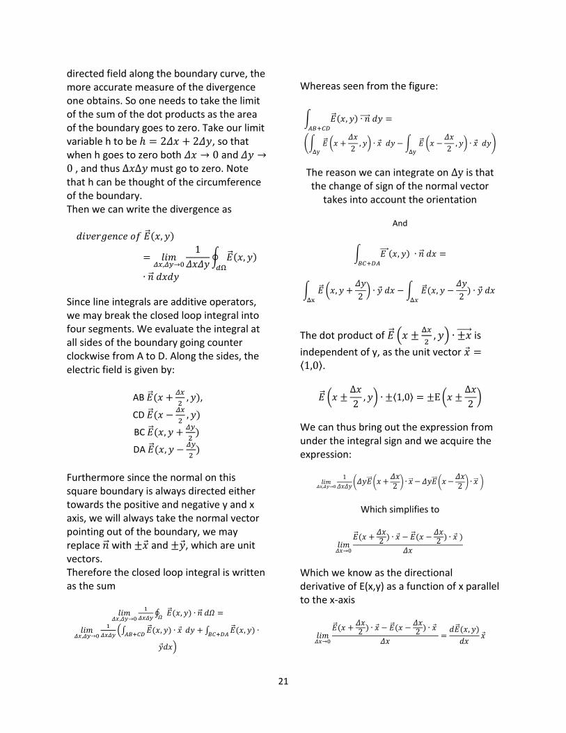
Now lets write this concept mathematically.
figure: Square boundary 𝛺 around point P.
Suppose �⃗⃗�(𝑥 , 𝑦) is a vector field in 𝑅2 . Now suppose we draw a square boundary around a point P and call the boundary 𝛺. Then the magnitude of the field normal to the boundary at every point along the boundary curve is given by the dot product
of the field �⃗⃗�(𝑥 , 𝑦) with the normal vector �⃗⃗�(𝑥, 𝑦) to the boundary curve. The dot
product �⃗⃗�(𝑥, 𝑦) ∙ �⃗⃗�(𝑥, 𝑦) can be seen as
the magnitude of the field �⃗⃗�(𝑥, 𝑦) in the direction of �⃗⃗�(𝑥, 𝑦).
Figure 2. Dot product: the dot product of the vector A and B is the length (magnitude) of A in the direction of B.
The smaller we let the boundary 𝑑Ω get and the more points we measure in the outward
21
directed field along the boundary curve, the more accurate measure of the divergence one obtains. So one needs to take the limit of the sum of the dot products as the area of the boundary goes to zero. Take our limit variable h to be ℎ = 2𝛥𝑥 + 2𝛥𝑦, so that when h goes to zero both 𝛥𝑥 → 0 and 𝛥𝑦 →0 , and thus Δ𝑥Δ𝑦 must go to zero. Note that h can be thought of the circumference of the boundary. Then we can write the divergence as
𝑑𝑖𝑣𝑒𝑟𝑔𝑒𝑛𝑐𝑒 𝑜𝑓 �⃗⃗�(𝑥, 𝑦)
= 𝑙𝑖𝑚𝛥𝑥,𝛥𝑦→0
1
𝛥𝑥𝛥𝑦∮ �⃗⃗�(𝑥, 𝑦)𝑑Ω
∙ �⃗⃗� 𝑑𝑥𝑑𝑦
Since line integrals are additive operators, we may break the closed loop integral into four segments. We evaluate the integral at all sides of the boundary going counter clockwise from A to D. Along the sides, the electric field is given by:
AB �⃗⃗�(𝑥 +𝛥𝑥
2, 𝑦),
CD �⃗⃗�(𝑥 −𝛥𝑥
2, 𝑦)
BC �⃗⃗�(𝑥, 𝑦 +𝛥𝑦
2)
DA �⃗⃗�(𝑥, 𝑦 −𝛥𝑦
2)
Furthermore since the normal on this square boundary is always directed either towards the positive and negative y and x axis, we will always take the normal vector pointing out of the boundary, we may replace �⃗⃗� with ±�⃗� and ±�⃗�, which are unit vectors. Therefore the closed loop integral is written as the sum
𝑙𝑖𝑚𝛥𝑥,𝛥𝑦→0
1
𝛥𝑥𝛥𝑦∮ �⃗⃗�(𝑥, 𝑦) ∙ �⃗⃗� 𝑑𝛺𝛺
=
𝑙𝑖𝑚𝛥𝑥,𝛥𝑦→0
1
𝛥𝑥𝛥𝑦(∫ �⃗⃗�(𝑥, 𝑦) ∙ �⃗� 𝐴𝐵+𝐶𝐷
𝑑𝑦 + ∫ �⃗⃗�(𝑥, 𝑦)𝐵𝐶+𝐷𝐴
∙
�⃗�𝑑𝑥)
Whereas seen from the figure:
∫ �⃗⃗�(𝑥, 𝑦) ∙ 𝑛⃗⃗⃗⃗⃗ 𝑑𝑦𝐴𝐵+𝐶𝐷
=
(∫ �⃗⃗� (𝑥 +𝛥𝑥
2, 𝑦) ∙ �⃗� 𝑑𝑦
Δy
−∫ �⃗⃗� (𝑥 −𝛥𝑥
2, 𝑦) ∙ �⃗� 𝑑𝑦
Δy
)
The reason we can integrate on Δy is that the change of sign of the normal vector
takes into account the orientation
And
∫ 𝐸 ⃗⃗⃗⃗ (𝑥, 𝑦) ∙ �⃗⃗� 𝑑𝑥𝐵𝐶+𝐷𝐴
=
∫ �⃗⃗� (𝑥, 𝑦 +𝛥𝑦
2) ∙ �⃗� 𝑑𝑥
Δx
−∫ �⃗⃗�(𝑥, 𝑦 −𝛥𝑦
2) ∙ �⃗� 𝑑𝑥
Δ𝑥
The dot product of �⃗⃗� (𝑥 ±Δ𝑥
2, 𝑦) ∙ ±𝑥⃗⃗⃗⃗⃗⃗ is
independent of y, as the unit vector �⃗� =⟨1,0⟩.
�⃗⃗� (𝑥 ±Δ𝑥
2, 𝑦) ∙ ±⟨1,0⟩ = ±E(𝑥 ±
Δ𝑥
2)
We can thus bring out the expression from under the integral sign and we acquire the expression:
𝑙𝑖𝑚𝛥𝑥,𝛥𝑦→0
1
𝛥𝑥𝛥𝑦(𝛥𝑦�⃗⃗⃗⃗�(𝑥+
𝛥𝑥2) ∙ �⃗⃗⃗� − 𝛥𝑦�⃗⃗⃗⃗� (𝑥−
𝛥𝑥2) ∙ �⃗⃗⃗� )
Which simplifies to
𝑙𝑖𝑚𝛥𝑥→0
�⃗⃗�(𝑥 +𝛥𝑥2) ∙ �⃗� − �⃗⃗�(𝑥 −
𝛥𝑥2) ∙ �⃗� )
𝛥𝑥
Which we know as the directional derivative of E(x,y) as a function of x parallel to the x-axis
𝑙𝑖𝑚𝛥𝑥→0
�⃗⃗�(𝑥 +𝛥𝑥2) ∙ �⃗� − �⃗⃗�(𝑥 −
𝛥𝑥2) ∙ �⃗�
𝛥𝑥=𝑑�⃗⃗�(𝑥, 𝑦)
𝑑𝑥�⃗�
22
By the same argument for the other sides of the boundary we obtain
𝑙𝑖𝑚𝛥𝑦→0
�⃗⃗�(𝑦 +𝛥𝑦2) ∙ 𝑦 − �⃗⃗�(𝑦 −
𝛥𝑦2) ∙ 𝑦 )
𝛥𝑦=𝑑�⃗⃗�(𝑥, 𝑦)
𝑑𝑦�⃗�
Note that these values are both scalars since it is the dot product of two vectors. We thus conclude that
𝑑𝑖𝑣𝑒𝑟𝑔𝑒𝑛𝑐𝑒 𝑜𝑓 �⃗⃗�(𝑥, 𝑦) =𝑑�⃗⃗�(𝑥, 𝑦)
𝑑𝑥�⃗� +
𝑑�⃗⃗�(𝑥, 𝑦)
𝑑𝑦�⃗�
or more compactly
𝛻�⃗⃗� =𝑑�⃗⃗�(𝑥, 𝑦)
𝑑𝑥�⃗� +
𝑑�⃗⃗�(𝑥, 𝑦)
𝑑𝑦�⃗�
Where 𝛻�⃗⃗� is known as the divergence of
the field�⃗⃗�. Divergence can in other words be estimated at any point as the scalar sum of the directional derivatives of the vector function, parallel to the vectors that span the space. [9]
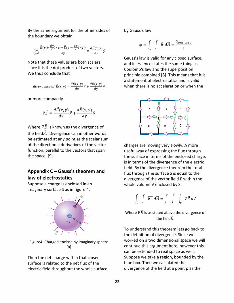
Appendix C – Gauss's theorem and law of electrostatics Suppose a charge is enclosed in an imaginary surface S as in figure 4.
Figure4: Charged enclose by imaginary sphere
[8]
Then the net charge within that closed surface is related to the net flux of the electric field throughout the whole surface
by Gauss’s law
𝜙 = ∫ ∫ �⃗⃗� 𝒅�⃗⃗⃗�𝑆
=𝑄𝑒𝑛𝑐𝑙𝑜𝑠𝑒𝑑
𝜖
Gauss’s law is valid for any closed surface, and in essence states the same thing as Coulomb's law and the superposition principle combined [8]. This means that it is a statement of electrostatics and is valid when there is no acceleration or when the
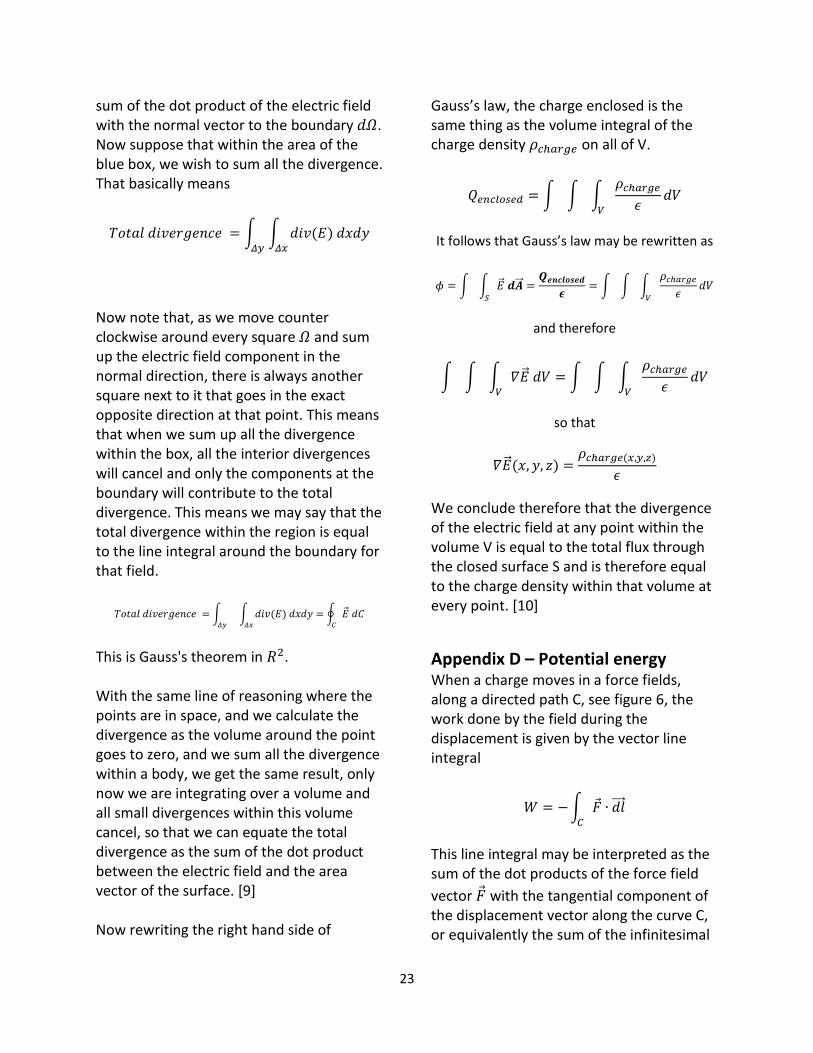
charges are moving very slowly. A more useful way of expressing the flux through the surface in terms of the enclosed charge, is in terms of the divergence of the electric field. By the divergence theorem the total flux through the surface S is equal to the divergence of the vector field E within the whole volume V enclosed by S.
∫ ∫ 𝐸 ∙⃗⃗ ⃗⃗⃗ 𝒅�⃗⃗⃗�𝑆
= ∫ ∫ ∫ 𝛻�⃗⃗� 𝑑𝑉𝑉
Where 𝛻�⃗⃗� is as stated above the divergence of
the field�⃗⃗�.
To understand this theorem lets go back to the definition of divergence. Since we worked on a two dimensional space we will continue this argument here, however this can be extended to real space as well. Suppose we take a region, bounded by the blue box. Then we calculated the divergence of the field at a point p as the
23
sum of the dot product of the electric field with the normal vector to the boundary 𝑑𝛺. Now suppose that within the area of the blue box, we wish to sum all the divergence. That basically means
𝑇𝑜𝑡𝑎𝑙 𝑑𝑖𝑣𝑒𝑟𝑔𝑒𝑛𝑐𝑒 = ∫ ∫ 𝑑𝑖𝑣(𝐸) 𝑑𝑥𝑑𝑦𝛥𝑥𝛥𝑦
Now note that, as we move counter clockwise around every square 𝛺 and sum up the electric field component in the normal direction, there is always another square next to it that goes in the exact opposite direction at that point. This means that when we sum up all the divergence within the box, all the interior divergences will cancel and only the components at the boundary will contribute to the total divergence. This means we may say that the total divergence within the region is equal to the line integral around the boundary for that field.
𝑇𝑜𝑡𝑎𝑙 𝑑𝑖𝑣𝑒𝑟𝑔𝑒𝑛𝑐𝑒 = ∫𝛥𝑦
∫ 𝑑𝑖𝑣(𝐸) 𝑑𝑥𝑑𝑦𝛥𝑥
= ∮ �⃗⃗� 𝑑𝐶𝐶
This is Gauss's theorem in 𝑅2. With the same line of reasoning where the points are in space, and we calculate the divergence as the volume around the point goes to zero, and we sum all the divergence within a body, we get the same result, only now we are integrating over a volume and all small divergences within this volume cancel, so that we can equate the total divergence as the sum of the dot product between the electric field and the area vector of the surface. [9] Now rewriting the right hand side of
Gauss’s law, the charge enclosed is the same thing as the volume integral of the charge density 𝜌𝑐ℎ𝑎𝑟𝑔𝑒 on all of V.
𝑄𝑒𝑛𝑐𝑙𝑜𝑠𝑒𝑑 = ∫ ∫ ∫𝜌𝑐ℎ𝑎𝑟𝑔𝑒
𝜖𝑑𝑉
𝑉
It follows that Gauss’s law may be rewritten as
𝜙 = ∫ ∫ �⃗⃗� 𝒅�⃗⃗⃗�𝑆
=𝑸𝒆𝒏𝒄𝒍𝒐𝒔𝒆𝒅
𝝐= ∫ ∫ ∫
𝜌𝑐ℎ𝑎𝑟𝑔𝑒
𝜖𝑑𝑉
𝑉
and therefore
∫ ∫ ∫ 𝛻�⃗⃗� 𝑑𝑉𝑉
= ∫ ∫ ∫𝜌𝑐ℎ𝑎𝑟𝑔𝑒
𝜖𝑑𝑉
𝑉
so that
𝛻�⃗⃗�(𝑥, 𝑦, 𝑧) =𝜌𝑐ℎ𝑎𝑟𝑔𝑒(𝑥,𝑦,𝑧)
𝜖
We conclude therefore that the divergence of the electric field at any point within the volume V is equal to the total flux through the closed surface S and is therefore equal to the charge density within that volume at every point. [10]
Appendix D – Potential energy When a charge moves in a force fields, along a directed path C, see figure 6, the work done by the field during the displacement is given by the vector line integral
𝑊 = −∫ �⃗� ∙ 𝑑𝑙⃗⃗⃗⃗𝐶
This line integral may be interpreted as the sum of the dot products of the force field
vector �⃗� with the tangential component of the displacement vector along the curve C, or equivalently the sum of the infinitesimal
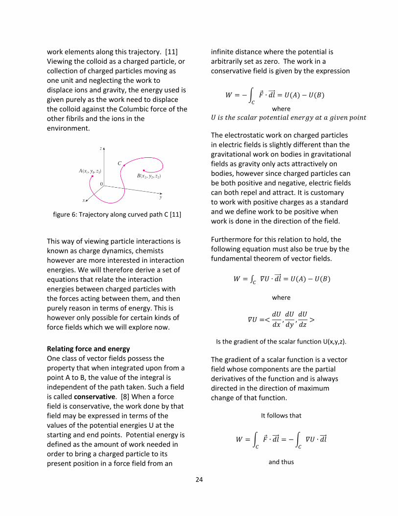
24
work elements along this trajectory. [11] Viewing the colloid as a charged particle, or collection of charged particles moving as one unit and neglecting the work to displace ions and gravity, the energy used is given purely as the work need to displace the colloid against the Columbic force of the other fibrils and the ions in the environment.
figure 6: Trajectory along curved path C [11]
This way of viewing particle interactions is known as charge dynamics, chemists however are more interested in interaction energies. We will therefore derive a set of equations that relate the interaction energies between charged particles with the forces acting between them, and then purely reason in terms of energy. This is however only possible for certain kinds of force fields which we will explore now.
Relating force and energy One class of vector fields possess the property that when integrated upon from a point A to B, the value of the integral is independent of the path taken. Such a field is called conservative. [8] When a force field is conservative, the work done by that field may be expressed in terms of the values of the potential energies U at the starting and end points. Potential energy is defined as the amount of work needed in order to bring a charged particle to its present position in a force field from an
infinite distance where the potential is arbitrarily set as zero. The work in a conservative field is given by the expression
𝑊 = −∫ �⃗� ∙ 𝑑𝑙⃗⃗⃗⃗𝐶
= 𝑈(𝐴) − 𝑈(𝐵)
where 𝑈 𝑖𝑠 𝑡ℎ𝑒 𝑠𝑐𝑎𝑙𝑎𝑟 𝑝𝑜𝑡𝑒𝑛𝑡𝑖𝑎𝑙 𝑒𝑛𝑒𝑟𝑔𝑦 𝑎𝑡 𝑎 𝑔𝑖𝑣𝑒𝑛 𝑝𝑜𝑖𝑛𝑡
The electrostatic work on charged particles in electric fields is slightly different than the gravitational work on bodies in gravitational fields as gravity only acts attractively on bodies, however since charged particles can be both positive and negative, electric fields can both repel and attract. It is customary to work with positive charges as a standard and we define work to be positive when work is done in the direction of the field.
Furthermore for this relation to hold, the following equation must also be true by the fundamental theorem of vector fields.
𝑊 = ∫ 𝛻𝑈 ∙ 𝑑𝑙⃗⃗⃗⃗𝐶
= 𝑈(𝐴) − 𝑈(𝐵)
where
𝛻𝑈 =<𝑑𝑈
𝑑𝑥,𝑑𝑈
𝑑𝑦,𝑑𝑈
𝑑𝑧>
Is the gradient of the scalar function U(x,y,z).
The gradient of a scalar function is a vector field whose components are the partial derivatives of the function and is always directed in the direction of maximum change of that function.
It follows that
𝑊 = ∫ �⃗� ∙ 𝑑𝑙⃗⃗⃗⃗𝐶
= −∫ 𝛻𝑈 ∙ 𝑑𝑙⃗⃗⃗⃗𝐶
and thus
25
�⃗� = −𝛻𝑈
This equation states that the force field always is directed towards lower potential energy. So essentially the force field will always move a particle to the position of lowest potential energy. This result bridges charge dynamics and energetics.
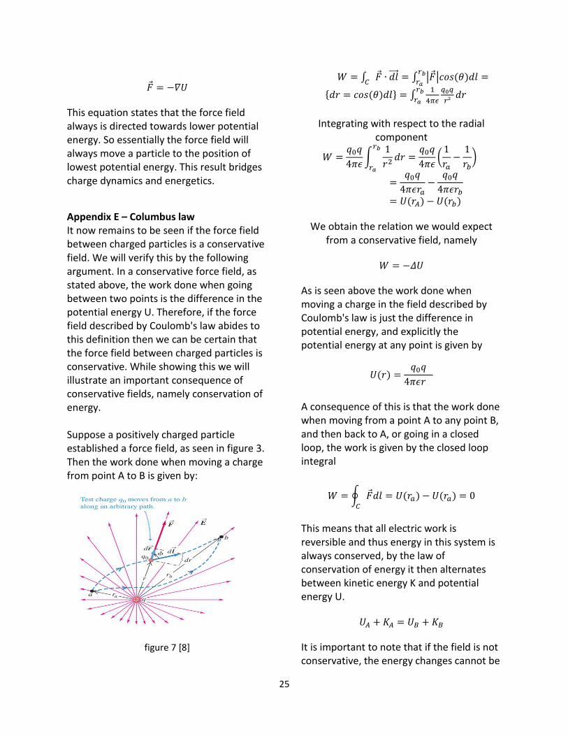
Appendix E – Columbus law It now remains to be seen if the force field between charged particles is a conservative field. We will verify this by the following argument. In a conservative force field, as stated above, the work done when going between two points is the difference in the potential energy U. Therefore, if the force field described by Coulomb's law abides to this definition then we can be certain that the force field between charged particles is conservative. While showing this we will illustrate an important consequence of conservative fields, namely conservation of energy. Suppose a positively charged particle established a force field, as seen in figure 3. Then the work done when moving a charge from point A to B is given by:
figure 7 [8]
𝑊 = ∫ �⃗� ∙ 𝑑𝑙⃗⃗⃗⃗𝐶
= ∫ |�⃗�|𝑐𝑜𝑠(𝜃)𝑑𝑙𝑟𝑏𝑟𝑎
=
{𝑑𝑟 = 𝑐𝑜𝑠(𝜃)𝑑𝑙} = ∫1
4𝜋𝜖
𝑞0𝑞
𝑟²𝑑𝑟
𝑟𝑏𝑟𝑎
Integrating with respect to the radial component
𝑊 =𝑞0𝑞
4𝜋𝜖∫
1
𝑟2𝑑𝑟
𝑟𝑏
𝑟𝑎
=𝑞0𝑞
4𝜋𝜖(1
𝑟𝑎−1
𝑟𝑏)
=𝑞0𝑞
4𝜋𝜖𝑟𝑎−
𝑞0𝑞
4𝜋𝜖𝑟𝑏= 𝑈(𝑟𝐴) − 𝑈(𝑟𝑏)
We obtain the relation we would expect from a conservative field, namely
𝑊 = −𝛥𝑈
As is seen above the work done when moving a charge in the field described by Coulomb's law is just the difference in potential energy, and explicitly the potential energy at any point is given by
𝑈(𝑟) =𝑞0𝑞
4𝜋𝜖𝑟
A consequence of this is that the work done when moving from a point A to any point B, and then back to A, or going in a closed loop, the work is given by the closed loop integral
𝑊 = ∮ �⃗�𝑑𝑙𝐶
= 𝑈(𝑟𝑎) − 𝑈(𝑟𝑎) = 0
This means that all electric work is reversible and thus energy in this system is always conserved, by the law of conservation of energy it then alternates between kinetic energy K and potential energy U.
𝑈𝐴 + 𝐾𝐴 = 𝑈𝐵 + 𝐾𝐵
It is important to note that if the field is not conservative, the energy changes cannot be
26
expressed as potential energies U but rather changes in internal energies. [8][11]
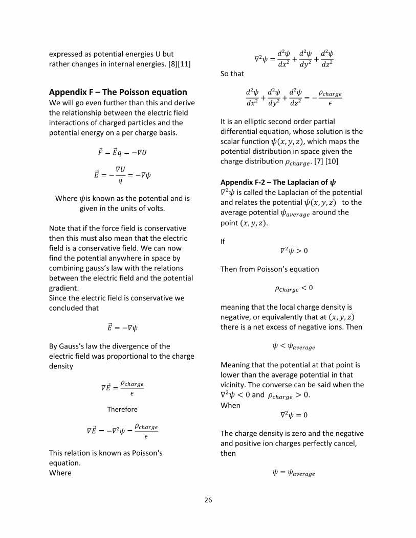
Appendix F – The Poisson equation We will go even further than this and derive the relationship between the electric field interactions of charged particles and the potential energy on a per charge basis.
�⃗� = �⃗⃗�𝑞 = −𝛻𝑈
�⃗⃗� = −𝛻𝑈
𝑞= −𝛻𝜓
Where 𝜓is known as the potential and is given in the units of volts.
Note that if the force field is conservative then this must also mean that the electric field is a conservative field. We can now find the potential anywhere in space by combining gauss’s law with the relations between the electric field and the potential gradient. Since the electric field is conservative we concluded that
�⃗⃗� = −𝛻𝜓
By Gauss’s law the divergence of the electric field was proportional to the charge density
𝛻�⃗⃗� =𝜌𝑐ℎ𝑎𝑟𝑔𝑒
𝜖
Therefore
𝛻�⃗⃗� = −𝛻²𝜓 =𝜌𝑐ℎ𝑎𝑟𝑔𝑒
𝜖
This relation is known as Poisson's equation. Where
∇2𝜓 =𝑑²𝜓
𝑑𝑥²+𝑑²𝜓
𝑑𝑦²+𝑑²𝜓
𝑑𝑧²
So that
𝑑²𝜓
𝑑𝑥²+𝑑²𝜓
𝑑𝑦²+𝑑²𝜓
𝑑𝑧²= −
𝜌𝑐ℎ𝑎𝑟𝑔𝑒
𝜖
It is an elliptic second order partial differential equation, whose solution is the scalar function 𝜓(𝑥, 𝑦, 𝑧), which maps the potential distribution in space given the charge distribution 𝜌𝑐ℎ𝑎𝑟𝑔𝑒. [7] [10]
Appendix F-2 – The Laplacian of 𝝍 𝛻²𝜓 is called the Laplacian of the potential and relates the potential 𝜓(𝑥, 𝑦, 𝑧) to the average potential 𝜓𝑎𝑣𝑒𝑟𝑎𝑔𝑒 around the
point (𝑥, 𝑦, 𝑧). If
𝛻2𝜓 > 0
Then from Poisson’s equation
𝜌𝐶ℎ𝑎𝑟𝑔𝑒 < 0
meaning that the local charge density is negative, or equivalently that at (𝑥, 𝑦, 𝑧) there is a net excess of negative ions. Then
𝜓 < 𝜓𝑎𝑣𝑒𝑟𝑎𝑔𝑒
Meaning that the potential at that point is lower than the average potential in that vicinity. The converse can be said when the ∇2𝜓 < 0 and 𝜌𝑐ℎ𝑎𝑟𝑔𝑒 > 0.
When ∇2𝜓 = 0
The charge density is zero and the negative and positive ion charges perfectly cancel, then
𝜓 = 𝜓𝑎𝑣𝑒𝑟𝑎𝑔𝑒
27
The potential at that point is equal to the average potential in that vicinity. [11] [12]
Appendix F-3 – Solution to Poisson’s equation What would we expect the potential drop to be like if we have no free ions? That is when 𝜌𝑐ℎ𝑎𝑟𝑔𝑒 = 0
∇2𝜓 = 0
Let’s for simplicity assume that 𝜓 only varies with x, so that we may say instead
𝑑2𝜓
𝑑𝑥2= 0
To solve for 𝜓 we integrate with respect to x, where x is the distance from the charged surface.
𝑑𝜓
𝑑𝑥= 𝐴
Where A is some integration constant, which we will determine with the boundary conditions. Integrating again to obtain 𝜓 we get
𝜓(𝑥) = 𝐴𝑥 + 𝐵
Now we impose the constraints that
𝜓(0) = 𝜓0 𝜓(𝑘) = 0
Meaning that the potential at the surface is the surface potential and that the potential drops to zero at some finite distance 𝑥 = 𝑘. Thus we see that when there are no free ions in the solution, Poisson’s equation predicts that the potential will drop linearly with distance from a charged surface.

28
Formation of the electrostatic double layer
29
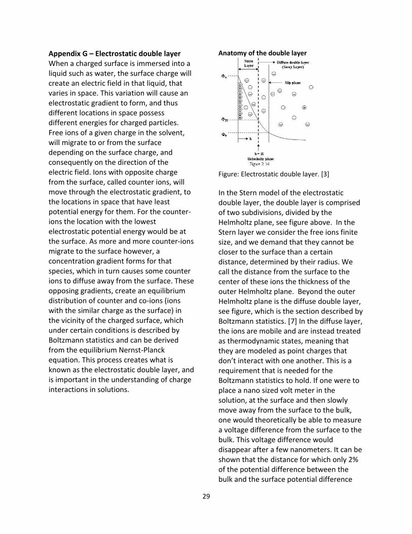
Appendix G – Electrostatic double layer When a charged surface is immersed into a liquid such as water, the surface charge will create an electric field in that liquid, that varies in space. This variation will cause an electrostatic gradient to form, and thus different locations in space possess different energies for charged particles. Free ions of a given charge in the solvent, will migrate to or from the surface depending on the surface charge, and consequently on the direction of the electric field. Ions with opposite charge from the surface, called counter ions, will move through the electrostatic gradient, to the locations in space that have least potential energy for them. For the counter-ions the location with the lowest electrostatic potential energy would be at the surface. As more and more counter-ions migrate to the surface however, a concentration gradient forms for that species, which in turn causes some counter ions to diffuse away from the surface. These opposing gradients, create an equilibrium distribution of counter and co-ions (ions with the similar charge as the surface) in the vicinity of the charged surface, which under certain conditions is described by Boltzmann statistics and can be derived from the equilibrium Nernst-Planck equation. This process creates what is known as the electrostatic double layer, and is important in the understanding of charge interactions in solutions.
Anatomy of the double layer
Figure: Electrostatic double layer. [3]
In the Stern model of the electrostatic double layer, the double layer is comprised of two subdivisions, divided by the Helmholtz plane, see figure above. In the Stern layer we consider the free ions finite size, and we demand that they cannot be closer to the surface than a certain distance, determined by their radius. We call the distance from the surface to the center of these ions the thickness of the outer Helmholtz plane. Beyond the outer Helmholtz plane is the diffuse double layer, see figure, which is the section described by Boltzmann statistics. [7] In the diffuse layer, the ions are mobile and are instead treated as thermodynamic states, meaning that they are modeled as point charges that don’t interact with one another. This is a requirement that is needed for the Boltzmann statistics to hold. If one were to place a nano sized volt meter in the solution, at the surface and then slowly move away from the surface to the bulk, one would theoretically be able to measure a voltage difference from the surface to the bulk. This voltage difference would disappear after a few nanometers. It can be shown that the distance for which only 2% of the potential difference between the bulk and the surface potential difference
30
remains is a property of only the bulk solution. The characteristic length for this interaction is called the Debye length and is discussed in Appendix J . For two charged surfaces in solution to interact electrostatically their double layers must overlap, thus this can only happen when the surfaces are within four Debye lengths of each other. [14]
Appendix H Flux density and diffusion
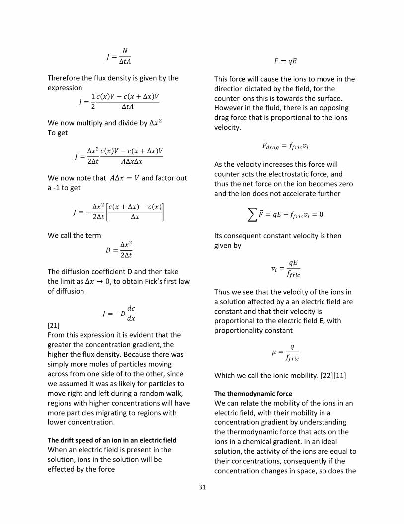
Convective flux density Consider a slab of area A and thickness Δ𝑥 and suppose the fluid stream has an ionic concentration of 𝑐𝑖.Then the number of moles of ions passing through the area in the figure below is given by the expression
𝑛 = 𝑐𝑉 = 𝑐𝐴Δ𝑥
Figure [5]
We then define the flux density as the number of particles per unit time Δ𝑡 and unit area 𝐴 as
𝐽𝑐𝑜𝑛𝑣𝑒𝑐𝑡𝑖𝑣𝑒 =𝑐𝐴Δ𝑥
Δ𝑡𝐴= 𝑐𝑖𝑣𝑖
[20] Diffusion and Fick’s first law
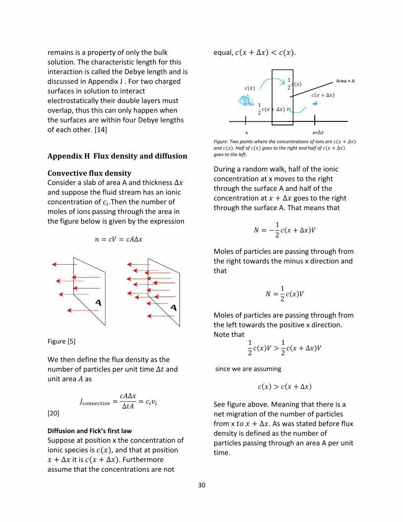
Suppose at position x the concentration of ionic species is 𝑐(𝑥), and that at position 𝑥 + Δ𝑥 it is 𝑐(𝑥 + Δ𝑥). Furthermore assume that the concentrations are not
equal, 𝑐(𝑥 + Δ𝑥) < 𝑐(𝑥).
Figure: Two points where the concentrations of ions are 𝑐(𝑥 + 𝛥𝑥) and 𝑐(𝑥). Half of 𝑐(𝑥) goes to the right and half of 𝑐(𝑥 + Δ𝑥) goes to the left.
During a random walk, half of the ionic concentration at x moves to the right through the surface A and half of the concentration at 𝑥 + Δ𝑥 goes to the right through the surface A. That means that
𝑁 = −1
2𝑐(𝑥 + Δ𝑥)𝑉
Moles of particles are passing through from the right towards the minus x direction and that
𝑁 =1
2𝑐(𝑥)𝑉
Moles of particles are passing through from the left towards the positive x direction. Note that
1
2𝑐(𝑥)𝑉 >
1
2𝑐(𝑥 + Δ𝑥)𝑉
since we are assuming
𝑐(𝑥) > 𝑐(𝑥 + Δ𝑥)
See figure above. Meaning that there is a net migration of the number of particles from x 𝑡𝑜 𝑥 + Δ𝑥. As was stated before flux density is defined as the number of particles passing through an area A per unit time.
31
𝐽 =𝑁
Δ𝑡𝐴
Therefore the flux density is given by the expression
𝐽 =1
2
𝑐(𝑥)𝑉 − 𝑐(𝑥 + Δ𝑥)𝑉
Δ𝑡𝐴
We now multiply and divide by Δ𝑥2 To get
𝐽 =Δ𝑥2
2Δ𝑡
𝑐(𝑥)𝑉 − 𝑐(𝑥 + Δ𝑥)𝑉
𝐴Δ𝑥Δ𝑥
We now note that 𝐴Δ𝑥 = 𝑉 and factor out a -1 to get
𝐽 = −Δ𝑥2
2Δ𝑡[𝑐(𝑥 + Δ𝑥) − 𝑐(𝑥)
Δ𝑥]
We call the term
𝐷 =Δ𝑥2
2Δ𝑡
The diffusion coefficient D and then take the limit as Δ𝑥 → 0, to obtain Fick’s first law of diffusion
𝐽 = −𝐷𝑑𝑐
𝑑𝑥
[21]
From this expression it is evident that the greater the concentration gradient, the higher the flux density. Because there was simply more moles of particles moving across from one side of to the other, since we assumed it was as likely for particles to move right and left during a random walk, regions with higher concentrations will have more particles migrating to regions with lower concentration. The drift speed of an ion in an electric field
When an electric field is present in the solution, ions in the solution will be effected by the force
𝐹 = 𝑞𝐸
This force will cause the ions to move in the direction dictated by the field, for the counter ions this is towards the surface. However in the fluid, there is an opposing drag force that is proportional to the ions velocity.
𝐹𝑑𝑟𝑎𝑔 = 𝑓𝑓𝑟𝑖𝑐𝑣𝑖
As the velocity increases this force will counter acts the electrostatic force, and thus the net force on the ion becomes zero and the ion does not accelerate further
∑�⃗� = 𝑞𝐸 −𝑓𝑓𝑟𝑖𝑐𝑣𝑖 = 0
Its consequent constant velocity is then given by
𝑣𝑖 =𝑞𝐸
𝑓𝑓𝑟𝑖𝑐
Thus we see that the velocity of the ions in a solution affected by a an electric field are constant and that their velocity is proportional to the electric field E, with proportionality constant
𝜇 =𝑞
𝑓𝑓𝑟𝑖𝑐
Which we call the ionic mobility. [22][11] The thermodynamic force
We can relate the mobility of the ions in an electric field, with their mobility in a concentration gradient by understanding the thermodynamic force that acts on the ions in a chemical gradient. In an ideal solution, the activity of the ions are equal to their concentrations, consequently if the concentration changes in space, so does the
32
chemical potential 𝜇𝑐ℎ𝑒𝑚, which is given by the expression
𝜇𝑐ℎ𝑒𝑚(𝑥) = 𝜇𝑐ℎ𝑒𝑚0 + 𝑅𝑇𝑙𝑛(𝑐(𝑥))
[22]
When an ion moves from a point x, the change in free energy is given by
Δ𝐺 = −𝜇𝑐ℎ𝑒𝑚1𝑑Δ
When that ion end up at a point 𝑥 + Δ𝑥 The free energy of that point is increased by
Δ𝐺 = 𝜇𝑐ℎ𝑒𝑚2Δ𝑛
Thus the change in free energy for the system for the particle to move from x to 𝑥 + Δ𝑥 is
Δ𝐺 = (𝜇𝑐ℎ𝑒𝑚2 − 𝜇𝑐ℎ𝑒𝑚1)Δ𝑛
In general the free energy is given by
Δ𝐺 = Δ𝐻 − 𝑇Δ𝑠 − 𝑆Δ𝑇
So that when temperature is constant Δ𝑇 =0
Δ𝐺 = Δ𝐻 − 𝑇Δ𝑆 Where
Δ𝐻 = Δ𝑤 + Δ𝑞 + Δ(𝑝𝑉)
Δ𝐺 = Δ𝑤 + Δ𝑞 + Δ(𝑝𝑉) − 𝑇Δ𝑠
So that we may write the change of free energy as
Δ𝐺 = Δ𝑤 + Δ𝑞 + Δ𝑝𝑉 + Δ𝑉𝑝 − 𝑇Δ𝑠
If the pressure is held constant Δ𝑝 = 0
Δ𝐺 = Δ𝑤 + Δ𝑞 + 𝑝Δ𝑉 − 𝑇Δ𝑠
And if the process is reversible, then
Δ𝑞 = 𝑇Δ𝑠
The work is made of two components, one expansion work component and one additional work component.
Δ𝑤 = Δ𝑤𝑒𝑥𝑝𝑎𝑛𝑠𝑖𝑜𝑛 + Δ𝑤𝑎𝑑𝑑𝑖𝑡𝑖𝑜𝑛𝑎𝑙
Where
Δ𝑤𝑒𝑥𝑝𝑎𝑛𝑠𝑖𝑜𝑛 = −𝑝Δ𝑉
Then the change is free energy is given by Δ𝐺 = −𝑝Δ𝑉 + Δ𝑤𝑎𝑑𝑑𝑖𝑡𝑖𝑜𝑛𝑎𝑙 + 𝑇Δ𝑆 − 𝑇Δ𝑠
+ 𝑝Δ𝑉
And so we conclude that the change in free energy at constant temperature and pressure is given by the additional work term. [22]
Δ𝐺 = Δ𝑤𝑎𝑑𝑑𝑖𝑡𝑖𝑜𝑛𝑎𝑙
We now see that at constant temperature and pressure the change in free energy of the system when moving an ion from x to 𝑥 + Δ𝑥 is
Δ𝑤𝑎𝑑𝑑 = (𝜇(𝑥 + Δ𝑥) − 𝜇(𝑥))Δ𝑛
We now take the work on a molar basis,
Δw′𝑎𝑑𝑑 =Δw𝑎𝑑𝑑
Δ𝑛 and multiply and divide by
Δx to obtain
Δw′𝑎𝑑𝑑 = [𝜇(𝑥 + Δ𝑥) − 𝜇(𝑥)
Δ𝑥] Δ𝑥
We then take the limit as Δ𝑥 → 0
𝑑𝑤𝑎𝑑𝑑′ = (
𝑑𝜇
𝑑𝑥)𝑑𝑥
We now notice that in general work is defined as force times distance
𝑑𝑤 = −𝐹𝑑𝑥
33
Which implies that the chemical gradient is a force that can do work.
𝐹 = −(𝑑𝜇
𝑑𝑥)
This force is known as the thermodynamic force [22]
If an ions chemical potential at a given temperature and pressure is
𝜇0
Then its chemical potential in a solution where there are other ionic species is given by
𝜇 = 𝜇0 + 𝑅𝑇𝑙𝑛(𝛼)
Where 𝛼 is the activity of that ionic species in the solution and can be seen as the effective mole fraction of that ionic species. [22] As was said in the beginning of this Appendix, If we assume that the chemical potential varies in space and that the solution is ideal, we can write the chemical potential as
𝜇𝑐ℎ𝑒𝑚(𝑥) = 𝜇𝑐ℎ𝑒𝑚0 + 𝑅𝑇𝑙𝑛(𝑐(𝑥))
We then differentiate with respect to x, using the chain rule and obtain the thermodynamic force 𝑑𝜇𝑐ℎ𝑒𝑚𝑑𝑥
= 𝑅𝑇𝑑
𝑑𝑥(ln(𝑐(𝑥))) = 𝑅𝑇 (
1
𝑐(𝑥))𝑑𝑐
𝑑𝑥
𝐹 = −(𝑑𝜇
𝑑𝑥) = −
𝑅𝑇
𝑐(𝑥)
𝑑𝑐
𝑑𝑥
[22]
Appendix H-1– The formation of the charge distribution We can now model the ions in the electrostatic double layer, we will begin by considering the change of concentration of
the counter ions with time 𝑑𝑐𝑖
𝑑𝑡 . Take the
control volume to be the diffuse part of the double layer, then the total flux j of ionic species is comprised of two components, one diffusive flux density 𝑗𝑑𝑖𝑓𝑓𝑢𝑠𝑖𝑣𝑒 and one
convective flux density 𝑗𝑐𝑜𝑛𝑣𝑒𝑐𝑡𝑖𝑣𝑒.
𝑗 = 𝑗𝑑𝑖𝑓𝑓𝑢𝑠𝑖𝑣𝑒 + 𝑗𝑐𝑜𝑛𝑣𝑒𝑐𝑡𝑖𝑣𝑒
By Fick’s first law of diffusion, the diffusive flux density is proportional to the concentration gradient of that species
𝑗𝑑𝑖𝑓𝑓𝑢𝑠𝑖𝑣𝑒 = −𝐷∇𝑐𝑖
Where D is the diffusion constant. The convective flux density is given by the product of the velocity and the concentration of that species.
𝑗𝑐𝑜𝑛𝑣𝑒𝑐𝑡𝑖𝑣𝑒 = 𝑣𝑖𝑐𝑖
The diffusive flux density is directed from the surface and arises due to that the counter ions accumulating on the charged surface create a concentration gradient ∇𝑐𝑖 that causes diffusion away from the surface. The convective flux is directed towards the charged surface for the counter ions and arises due to that counter ions have a velocity in the electric field that is directed towards the surface. When there is an electric field involved the velocity of the ions is given by the sum of the fluid velocity and the relative velocity of the ions to the fluid due to the electric field.
𝑣𝑖 = 𝑣𝑓𝑙𝑢𝑖𝑑 + 𝜇𝑖 �⃗⃗�
Where 𝜇 is the mobility of the ion in that
34
fluid. Since the fluid velocity is zero at the double layer we instead write
𝑣𝑖 = 𝜇𝑖 �⃗⃗�
Where 𝜇 is the ionic mobility that was discussed previously. The change of concentration of the species in the control volume with time is determined by how much flux density is converging in through the boundary surface. By converging we refer to the negative of the divergence operator -∇, that was discussed in Appendix B.
𝑑𝑐𝑖𝑑𝑡
= −∇𝑗
This equation is called the Nernst-Planck equation. At equilibrium, the change of concentration in the double layer with time is zero. Therefor we get that
−∇[𝑗𝑑𝑖𝑓𝑓𝑢𝑠𝑖𝑣𝑒 + 𝑗𝑐𝑜𝑛𝑣𝑒𝑐𝑡𝑖𝑣𝑒] = 0
And therefore
𝑗𝑐𝑜𝑛𝑣𝑒𝑐𝑡𝑖𝑣𝑒 = 𝑗𝑑𝑖𝑓𝑓𝑢𝑠𝑖𝑣𝑒
Meaning that that at equilibrium the convective flux is equal to the diffusive flux. By substituting in Ficks law and the velocity of the ions in the electric field to the expressions we get the relation
𝐷𝑑𝑐
𝑑𝑥= 𝜇�⃗⃗�𝑐𝑖
In order to solve this for 𝑐(𝑥), we need to relate the ions mobility in the electrostatic gradient 𝜇 with the ions mobility in the chemical gradient. To do this we first substitute in the thermodynamic force that
was discussed in the previous section for 𝑑𝑐
𝑑𝑥.
Recall that
𝐹 = −𝑅𝑇
𝑐(𝑥)
𝑑𝑐
𝑑𝑥
So that 𝑑𝑐
𝑑𝑥=𝑐𝐹
𝑅𝑇
Substituting this into the relation above we get
𝐷𝑐𝑖𝐹
𝑅𝑇= 𝜇�⃗⃗�𝑐𝑖
If we now assume that we are working with point charges, and thus neglect the ions dipoles, so that they won’t rotate in an electric field and neglect their finite size we can relate the thermodynamic force with the electrostatic [14] [22] force on a molar basis
𝐹 = 𝑞𝑖𝐹𝐴𝐸
where 𝐹𝐴 is the Faraday constant
𝐹𝑒𝑙𝑒𝑐𝑡𝑟𝑜 = 𝐹𝑡ℎ𝑒𝑟𝑚𝑜
𝐹 = 𝑞𝐸 =𝑅𝑇
𝑐(𝑥)
𝑑𝑐
𝑑𝑥
Then we can substitute 𝑞𝑖𝐹𝐴𝐸 , for F and obtain
𝐷𝑞𝑖𝐹𝐴𝐸
𝑅𝑇= 𝜇𝐸
We then divide by E and 𝐹𝐴𝑞𝑖 to obtain
𝐷
𝑅𝑇=
𝜇
𝐹𝐴𝑞𝑖
This relation is known as the Nernst-Einstein relation. [14] It relates Diffusion which is the movement of particles in a chemical gradient to the electrostatic mobility 𝜇 which is the movement of charged particles in an electrostatic
35
gradient.
Going back to our equilibrium relation
𝐷𝑑𝑐
𝑑𝑥= 𝜇�⃗⃗�𝑐𝑖
We divide by D and c and multiply both sides by dx to obtain.
𝑑𝑐
𝑐=𝜇�⃗⃗�
𝐷𝑑𝑥
We then solve for 𝐷 in the Nernst-Einstein relation
𝐷 =𝑅𝑇𝜇
𝑞𝑖𝐹𝐴
And substitute for the diffusion constant D. Then we get that
𝑑𝑐
𝑐=𝐹𝐴𝑞𝑖�⃗⃗�
𝑅𝑇𝑑𝑥
Now recall from Appendix A that the force is equal to the charge times the electric
field, on a per mole basis this is
�⃗� = 𝑞𝑖𝐹𝐴�⃗⃗�
So we get that
𝑑𝑐
𝑐=𝐹𝐴𝑞𝑖�⃗�
𝑅𝑇𝑑𝑥
Now if the electric force field �⃗� is a conservative field, as was discussed in Appendix D, then we can say that the
integral of the force with respect to the spatial variable x, along some displacement
is equal to the difference in potential energy between the starting and end
locations
𝑊 = −∫ �⃗� ∙ 𝑑𝑙⃗⃗⃗⃗𝐶
= 𝑈(𝐴) − 𝑈(𝐵)
Take the potential energy in the bulk to be zero since we impose the condition that
lim𝑥→𝑅≫𝜅−1
𝜓 (𝑥) = 0
Then the work to move an ion from the bulk to the distance x from the surface is given by
𝑊 = −𝑈(𝐴) = −𝑒𝑞𝑖𝜓(𝑥)
So that when we integrate both sides of
∫𝑑𝑐
𝑐
𝑐𝑖
𝑐0
=𝐹𝐴𝑅𝑇
∫ �⃗�𝑥
𝑅
𝑑𝑥
Where 𝑐0 is the bulk concentration
We obtain
ln (𝑐𝑖𝑐0) = −
𝐹𝐴𝑅𝑇
𝑒𝑞𝑖𝜓(𝑥)
And thus 𝑐𝑖𝑐0= 𝑒−
𝐹𝐴𝑞𝑒𝜓(𝑥)𝑅𝑇
To get this in a more familiar form we note that
𝐹𝐴𝑅=1
𝑘𝐵
Thus we obtain that
𝑐𝑖 = 𝑐0𝑒−𝑞𝑖𝑒𝜓(𝑥)𝑘𝐵𝑇
Meaning that the ionic concentration in the diffuse double layer at equilibrium when treating the ions as point charges is described by a Boltzmann distribution. [11][14] [20]

Boltzmann distributions
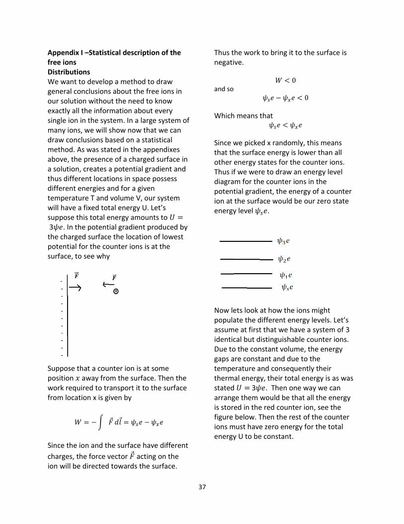
37
Appendix I –Statistical description of the free ions Distributions We want to develop a method to draw general conclusions about the free ions in our solution without the need to know exactly all the information about every single ion in the system. In a large system of many ions, we will show now that we can draw conclusions based on a statistical method. As was stated in the appendixes above, the presence of a charged surface in a solution, creates a potential gradient and thus different locations in space possess different energies and for a given temperature T and volume V, our system will have a fixed total energy U. Let’s suppose this total energy amounts to 𝑈 = 3𝜓𝑒. In the potential gradient produced by the charged surface the location of lowest potential for the counter ions is at the surface, to see why
Suppose that a counter ion is at some position 𝑥 away from the surface. Then the work required to transport it to the surface from location x is given by
𝑊 = −∫ �⃗� 𝑑𝑙 = 𝜓𝑠𝑒 − 𝜓𝑥𝑒
Since the ion and the surface have different
charges, the force vector �⃗� acting on the ion will be directed towards the surface.
Thus the work to bring it to the surface is negative.
𝑊 < 0 and so
𝜓𝑠𝑒 − 𝜓𝑥𝑒 < 0
Which means that 𝜓𝑠𝑒 < 𝜓𝑥𝑒
Since we picked x randomly, this means that the surface energy is lower than all other energy states for the counter ions. Thus if we were to draw an energy level diagram for the counter ions in the potential gradient, the energy of a counter ion at the surface would be our zero state energy level 𝜓𝑠𝑒.
Now lets look at how the ions might populate the different energy levels. Let’s assume at first that we have a system of 3 identical but distinguishable counter ions. Due to the constant volume, the energy gaps are constant and due to the temperature and consequently their thermal energy, their total energy is as was stated 𝑈 = 3𝜓𝑒. Then one way we can arrange them would be that all the energy is stored in the red counter ion, see the figure below. Then the rest of the counter ions must have zero energy for the total energy U to be constant.
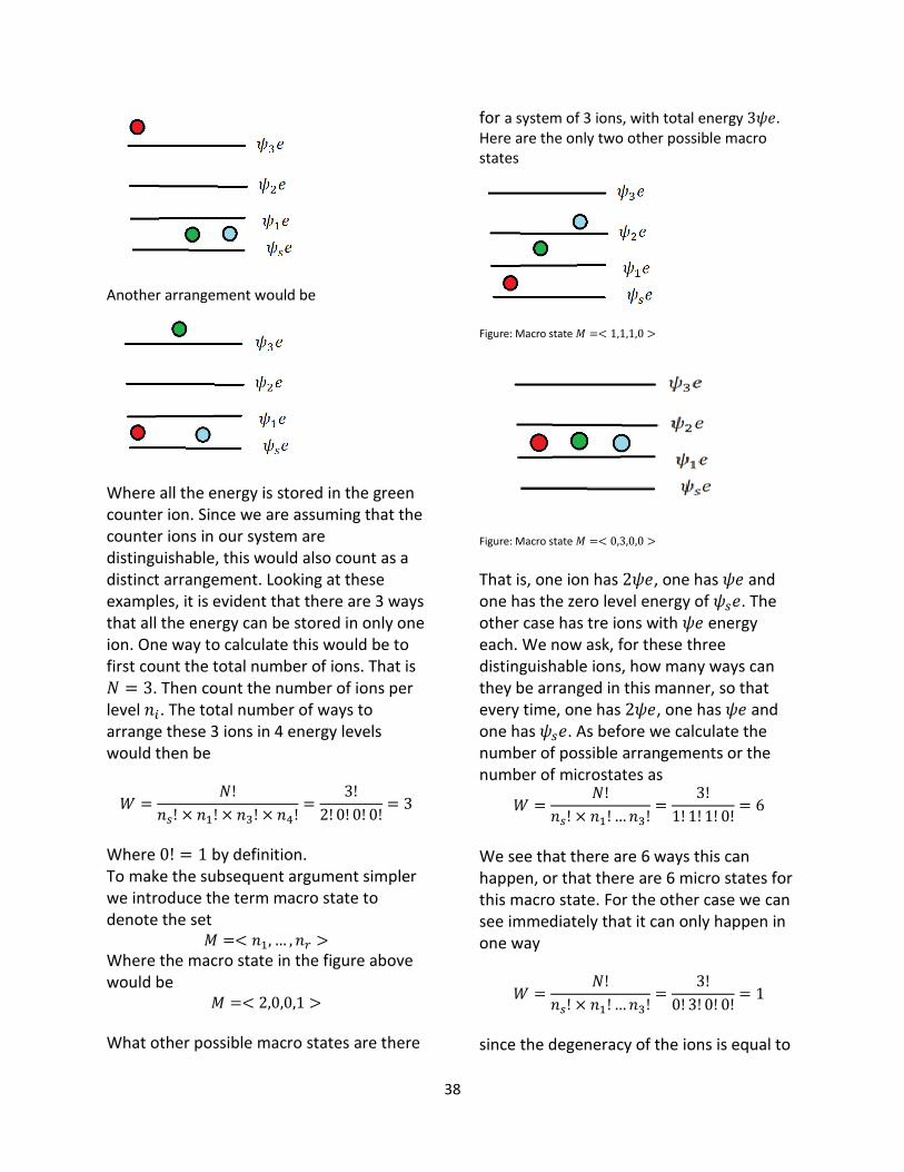
38
Another arrangement would be
Where all the energy is stored in the green counter ion. Since we are assuming that the counter ions in our system are distinguishable, this would also count as a distinct arrangement. Looking at these examples, it is evident that there are 3 ways that all the energy can be stored in only one ion. One way to calculate this would be to first count the total number of ions. That is 𝑁 = 3. Then count the number of ions per level 𝑛𝑖. The total number of ways to arrange these 3 ions in 4 energy levels would then be
𝑊 =𝑁!
𝑛𝑠! × 𝑛1! × 𝑛3! × 𝑛4!=
3!
2! 0! 0! 0!= 3
Where 0! = 1 by definition. To make the subsequent argument simpler we introduce the term macro state to denote the set
𝑀 =< 𝑛1, … , 𝑛𝑟 >
Where the macro state in the figure above would be
𝑀 =< 2,0,0,1 >
What other possible macro states are there
for a system of 3 ions, with total energy 3𝜓𝑒. Here are the only two other possible macro states
Figure: Macro state 𝑀 =< 1,1,1,0 >
Figure: Macro state 𝑀 =< 0,3,0,0 >
That is, one ion has 2𝜓𝑒, one has 𝜓𝑒 and one has the zero level energy of 𝜓𝑠𝑒. The other case has tre ions with 𝜓𝑒 energy each. We now ask, for these three distinguishable ions, how many ways can they be arranged in this manner, so that every time, one has 2𝜓𝑒, one has 𝜓𝑒 and one has 𝜓𝑠𝑒. As before we calculate the number of possible arrangements or the number of microstates as
𝑊 =𝑁!
𝑛𝑠! × 𝑛1!…𝑛3!=
3!
1! 1! 1! 0!= 6
We see that there are 6 ways this can happen, or that there are 6 micro states for this macro state. For the other case we can see immediately that it can only happen in one way
𝑊 =𝑁!
𝑛𝑠! × 𝑛1!…𝑛3!=
3!
0! 3! 0! 0!= 1
since the degeneracy of the ions is equal to
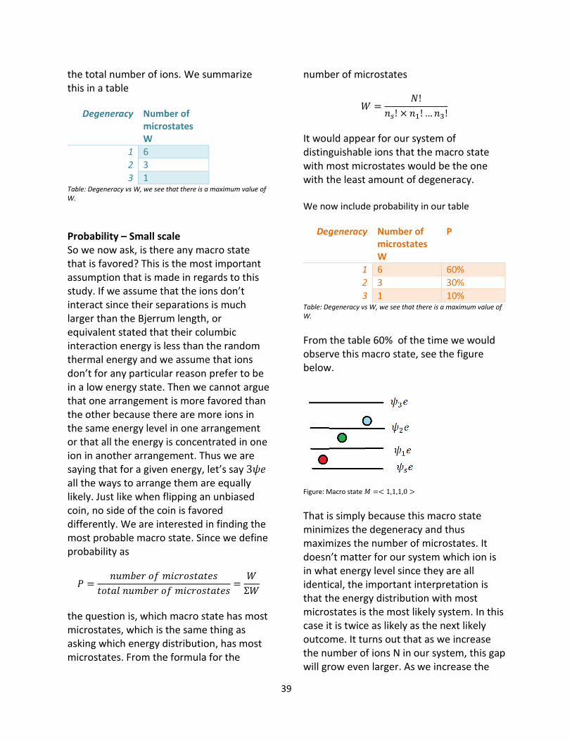
39
the total number of ions. We summarize this in a table
Degeneracy Number of microstates W
1 6
2 3
3 1 Table: Degeneracy vs W, we see that there is a maximum value of W.
Probability – Small scale So we now ask, is there any macro state that is favored? This is the most important assumption that is made in regards to this study. If we assume that the ions don’t interact since their separations is much larger than the Bjerrum length, or equivalent stated that their columbic interaction energy is less than the random thermal energy and we assume that ions don’t for any particular reason prefer to be in a low energy state. Then we cannot argue that one arrangement is more favored than the other because there are more ions in the same energy level in one arrangement or that all the energy is concentrated in one ion in another arrangement. Thus we are saying that for a given energy, let’s say 3𝜓𝑒 all the ways to arrange them are equally likely. Just like when flipping an unbiased coin, no side of the coin is favored differently. We are interested in finding the most probable macro state. Since we define probability as
𝑃 =𝑛𝑢𝑚𝑏𝑒𝑟 𝑜𝑓 𝑚𝑖𝑐𝑟𝑜𝑠𝑡𝑎𝑡𝑒𝑠
𝑡𝑜𝑡𝑎𝑙 𝑛𝑢𝑚𝑏𝑒𝑟 𝑜𝑓 𝑚𝑖𝑐𝑟𝑜𝑠𝑡𝑎𝑡𝑒𝑠=𝑊
Σ𝑊
the question is, which macro state has most microstates, which is the same thing as asking which energy distribution, has most microstates. From the formula for the
number of microstates
𝑊 =𝑁!
𝑛𝑠! × 𝑛1! …𝑛3!
It would appear for our system of distinguishable ions that the macro state with most microstates would be the one with the least amount of degeneracy. We now include probability in our table
Degeneracy Number of microstates W
P
1 6 60%
2 3 30%
3 1 10% Table: Degeneracy vs W, we see that there is a maximum value of W.
From the table 60% of the time we would observe this macro state, see the figure below.
Figure: Macro state 𝑀 =< 1,1,1,0 >
That is simply because this macro state minimizes the degeneracy and thus maximizes the number of microstates. It doesn’t matter for our system which ion is in what energy level since they are all identical, the important interpretation is that the energy distribution with most microstates is the most likely system. In this case it is twice as likely as the next likely outcome. It turns out that as we increase the number of ions N in our system, this gap will grow even larger. As we increase the
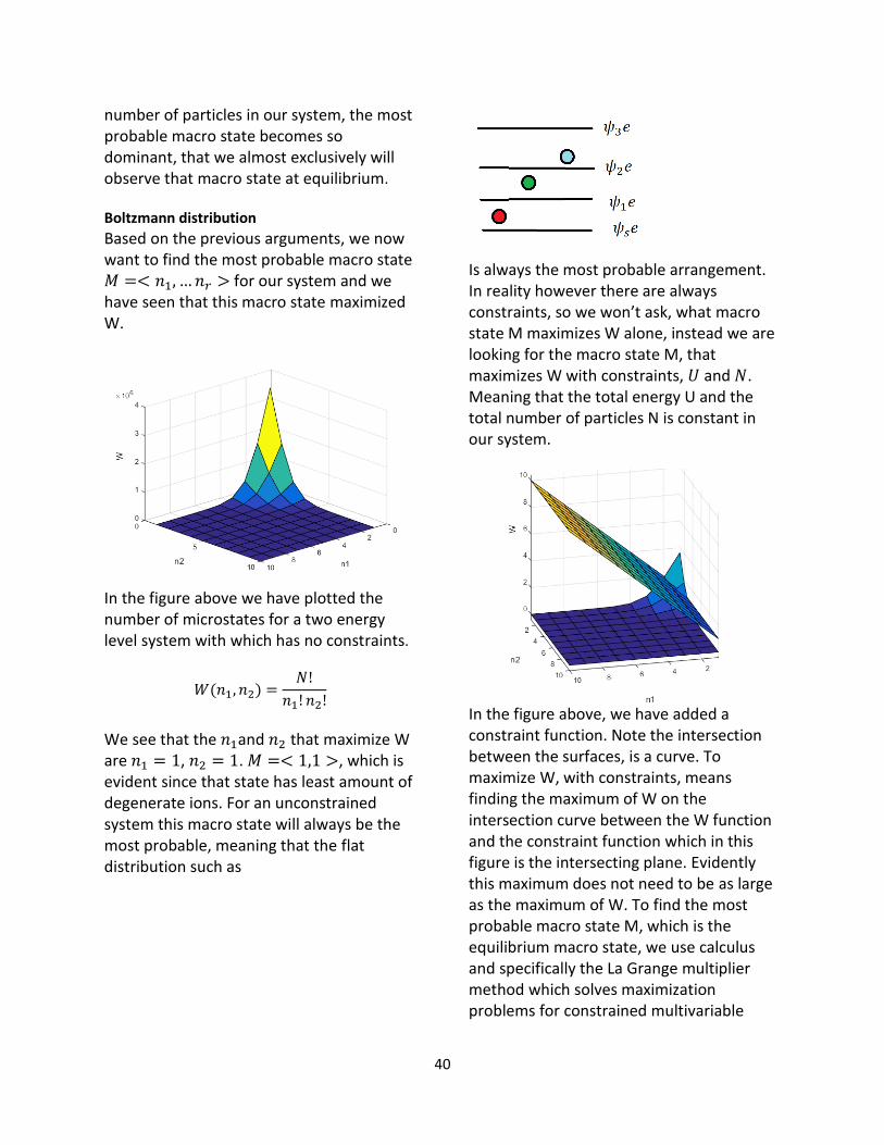
40
number of particles in our system, the most probable macro state becomes so dominant, that we almost exclusively will observe that macro state at equilibrium. Boltzmann distribution
Based on the previous arguments, we now want to find the most probable macro state 𝑀 =< 𝑛1, … 𝑛𝑟 > for our system and we have seen that this macro state maximized W.
In the figure above we have plotted the number of microstates for a two energy level system with which has no constraints.
𝑊(𝑛1, 𝑛2) =𝑁!
𝑛1! 𝑛2!
We see that the 𝑛1and 𝑛2 that maximize W are 𝑛1 = 1, 𝑛2 = 1. 𝑀 =< 1,1 >, which is evident since that state has least amount of degenerate ions. For an unconstrained system this macro state will always be the most probable, meaning that the flat distribution such as
Is always the most probable arrangement. In reality however there are always constraints, so we won’t ask, what macro state M maximizes W alone, instead we are looking for the macro state M, that maximizes W with constraints, 𝑈 and 𝑁. Meaning that the total energy U and the total number of particles N is constant in our system.
In the figure above, we have added a constraint function. Note the intersection between the surfaces, is a curve. To maximize W, with constraints, means finding the maximum of W on the intersection curve between the W function and the constraint function which in this figure is the intersecting plane. Evidently this maximum does not need to be as large as the maximum of W. To find the most probable macro state M, which is the equilibrium macro state, we use calculus and specifically the La Grange multiplier method which solves maximization problems for constrained multivariable
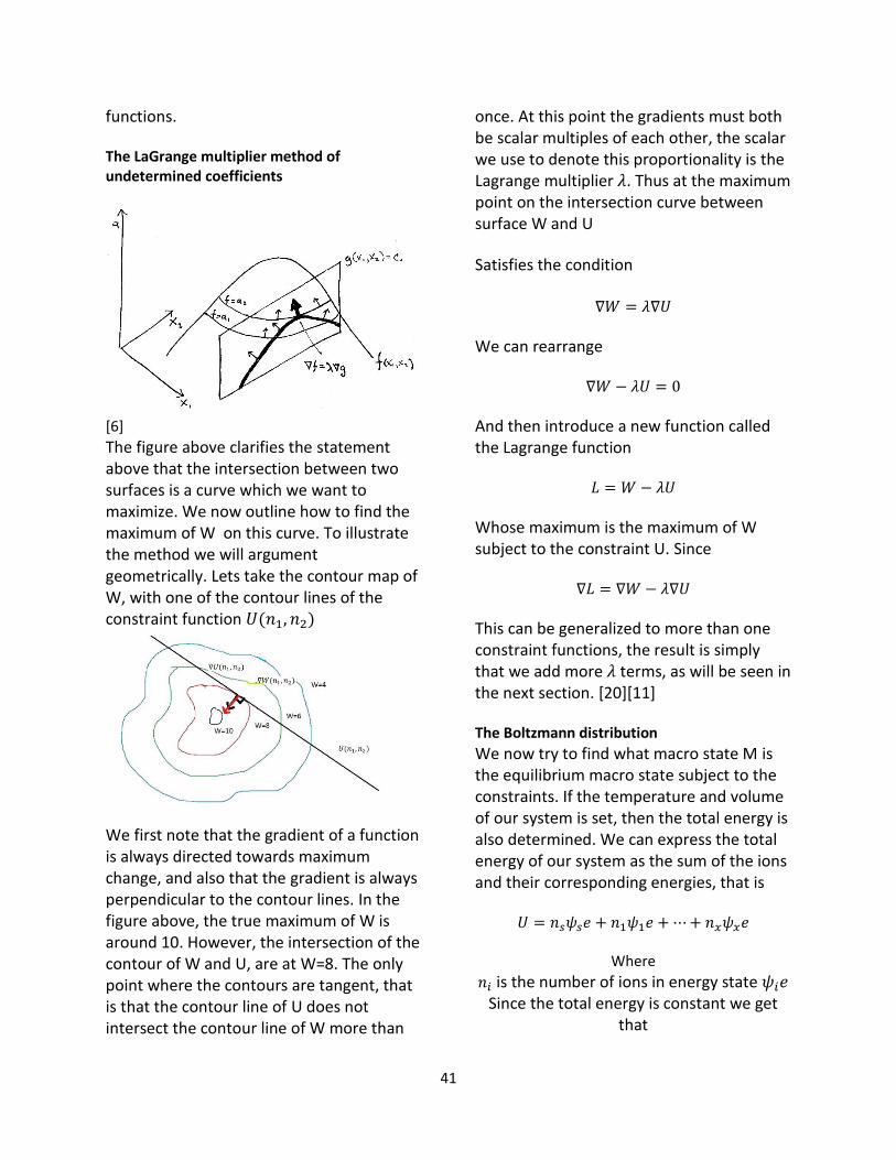
41
functions. The LaGrange multiplier method of undetermined coefficients
[6]
The figure above clarifies the statement above that the intersection between two surfaces is a curve which we want to maximize. We now outline how to find the maximum of W on this curve. To illustrate the method we will argument geometrically. Lets take the contour map of W, with one of the contour lines of the constraint function 𝑈(𝑛1, 𝑛2)
We first note that the gradient of a function is always directed towards maximum change, and also that the gradient is always perpendicular to the contour lines. In the figure above, the true maximum of W is around 10. However, the intersection of the contour of W and U, are at W=8. The only point where the contours are tangent, that is that the contour line of U does not intersect the contour line of W more than
once. At this point the gradients must both be scalar multiples of each other, the scalar we use to denote this proportionality is the Lagrange multiplier 𝜆. Thus at the maximum point on the intersection curve between surface W and U
Satisfies the condition
∇𝑊 = 𝜆∇𝑈
We can rearrange
∇𝑊 − 𝜆𝑈 = 0
And then introduce a new function called the Lagrange function
𝐿 = 𝑊 − 𝜆𝑈
Whose maximum is the maximum of W subject to the constraint U. Since
∇𝐿 = ∇𝑊 − 𝜆∇𝑈
This can be generalized to more than one constraint functions, the result is simply that we add more 𝜆 terms, as will be seen in the next section. [20][11] The Boltzmann distribution
We now try to find what macro state M is the equilibrium macro state subject to the constraints. If the temperature and volume of our system is set, then the total energy is also determined. We can express the total energy of our system as the sum of the ions and their corresponding energies, that is
𝑈 = 𝑛𝑠𝜓𝑠𝑒 + 𝑛1𝜓1𝑒 +⋯+ 𝑛𝑥𝜓𝑥𝑒
Where
𝑛𝑖 is the number of ions in energy state 𝜓𝑖𝑒 Since the total energy is constant we get
that
42
𝑑𝑈 = 0
We constrain the number of particles in our system at equilibrium so that the total number of particles is fixed
𝑁 = 𝑛𝑠 + 𝑛1 +⋯+ 𝑛𝑥
𝑑𝑁 = 0
To find the most likely micro state subject to these constrains, we maximize W with constraint N and U, so our Lagrange equation becomes
𝐿 = 𝑊 + 𝜆1𝑁 + 𝜆2𝑈
To maximize L we require that the partial derivative of L with respect to all the variables 𝑛𝑠, … , 𝑛𝑥 is zero
𝑑𝐿
𝑑𝑛𝑖= 0
For 𝑖 = 𝑠,… . , 𝑥, simultaneously.
As it stands however, W is hard to differentiate, since it contains factorials
𝑊 =𝑁!
𝑛𝑠!, … . 𝑛𝑥!
To work around this we first take the logarithm of W, which does not change M, since the maximum of ln (𝑊) is also the maximum of W. We then use the Sterling approximation, to simplify and get rid of the factorial terms. First note that
ln(𝑥𝑦) = ln(𝑥) + ln(𝑦) And
ln (𝑥
𝑦) = ln(𝑥) − ln (𝑦)
So that we may rewrite the natural logarithm of W as ln(𝑊) = ln(𝑁!) − (ln(𝑛𝑠!) + ⋯+ ln(𝑛𝑥!))
Now note that by the Sterling approximation
ln(𝑥!) = 𝑥𝑙𝑛(𝑥) − 𝑥 [23] So 𝑙𝑛(𝑊) becomes ln(𝑊) = 𝑁𝑙𝑛(𝑁) − 𝑁 − (𝑛𝑆 ln(𝑛𝑠) − 𝑛𝑠+. . +) Equivalently
ln(𝑊) = 𝑁𝑙𝑛(𝑁) − 𝑁 −∑𝑛𝑖 ln(𝑛𝑖) − 𝑛_𝑖
𝑥
𝑖=𝑠
Which is an expression without the
factorials. Since we require that 𝑑𝐿
𝑑𝑛= 0 for
all independent variables simultaneously we now differentiate with respect to all n, and then set those equations equal to zero to find the maximum. 𝑑𝐿
𝑑𝑛𝑖=
𝑑
𝑑𝑛𝑖(𝑁𝑙𝑛(𝑁) − 𝑁 − 𝑁𝑙𝑛(𝑁) − 𝑁
−∑𝑛𝑖 ln(𝑛𝑖) − 𝑛𝑖
𝑥
𝑖=𝑠
+𝑑
𝑑𝑛𝑖(𝜆1𝑁) +
𝑑
𝑑𝑛𝑖(𝜆2𝑈) = 0
For 𝑖 = 𝑠,… , 𝑥
To simplify things we break it up into parts. Where the first part is taken as
𝑑
𝑑𝑛𝑖(𝑁𝑙𝑛(𝑁) − 𝑁 − 𝑁𝑙𝑛(𝑁) − 𝑁
−∑𝑛𝑖 ln(𝑛𝑖) − 𝑛𝑖
𝑥
𝑖=𝑠
)
Since N is just a constant that whole term
43
becomes zero when we are differentiating with respect to 𝑛𝑖. Likewise in the sum, only the 𝑛𝑖 term remains, and all other terms in the sum go to zero, so we can simplify and say
𝑑
𝑑𝑛𝑖(𝑁𝑙𝑛(𝑁) − 𝑁 −∑𝑛𝑖 ln(𝑛𝑖) − 𝑛𝑖
𝑥
𝑖=𝑠
) =
0 −𝑑
𝑑𝑛𝑖(𝑛𝑖 ln(𝑛𝑖) − 𝑛𝑖)
We then use the product rule and get
−(1 ln(𝑛𝑖) +𝑛𝑖ni− 1)
So that the first part of the differential is just
−ln (𝑛𝑖)
We now differentiate
𝑑
𝑑𝑛𝑖(𝜆2𝑈)
Recalling that the total energy is just the number of ions per energy state, times the energy of those corresponding energy states. 𝑈 = 𝑛𝑠𝜓𝑠𝑒 +⋯+ 𝑛𝑥𝜓𝑥𝑒 = ∑ 𝑛𝑖𝜓𝑖𝑒
𝑟𝑖=𝑠
Again when differentiating with respect to 𝑛𝑖 we see that all the terms in the sum turn to zero except the term involving 𝑛𝑖, so we see that
𝑑
𝑑𝑛𝑖(𝜆2∑ 𝑛𝑖𝜓𝑖𝑒
𝑟
𝑖=𝑠) = 𝜆2𝜓𝑖𝑒
We now differentiate the last term 𝑑
𝑑𝑛𝑖(𝜆1𝑁)
Recall that
𝑁 = 𝑛𝑠+. . +𝑛𝑥 =∑𝑛𝑖
𝑥
𝑖=𝑠
So that only the 𝑛𝑖 term remains and we get that
𝑑
𝑑𝑛𝑖(𝜆1∑𝑛𝑖
𝑥
𝑖=𝑠
) = 𝜆1
So the total expression for the partial derivative of L with respect to 𝑛𝑖 would be at the maximum would be
𝑑𝐿
𝑑𝑛𝑖= − ln(𝑛𝑖) + 𝜆1 + 𝜆2𝜓𝑖𝑒 = 0
If we solve for ln (𝑛𝑖)
ln(𝑛𝑖) = 𝜆1 + 𝜆2𝜓𝑖𝑒
And then for 𝑛𝑖 it self we get
𝑛𝑖 = 𝑒𝜆1+𝜆2𝜓𝑖𝑒
We now need to determine the Lagrange multipliers 𝜆1 and 𝜆2.
We begin with 𝜆2, since it will create a connection to entropy and has most significance for this work. The undetermined Lagrange coefficient 𝝀𝟐
We first assume that we have found the macro state 𝑀 =< 𝑛𝑠 , . . , 𝑛𝑥 > that maximized the Lagrange function L and then consider what happens if we alter the system a little by adding a little heat energy 𝑑𝑄 that it so small that it does not alter the macro state M, or equivalently said we add just enough heat energy so that no ions change energy levels. Since we are at the maximum even after a small addition of heat energy 𝑑𝑄
44
𝑑𝐿 = 0
The expression for dL is as before
𝑑𝐿 = 𝑑𝑙𝑛(𝑊) + 𝜆1𝑑𝑁 + 𝜆2𝑑𝑈
Since we are assuming that no rearrangements are occurring after the addition of 𝑑𝑄.
𝑑𝑁 = 0 So that
𝑑𝐿 = 𝑑𝑙𝑛(𝑊) + 𝜆2𝑑𝑈
Where by the first law of thermodynamics the change in internal energy is equal to the change in work and heat energy. [23]
𝑑𝑈 = 𝑑𝑄 + 𝑑𝑤
Where the work 𝑑𝑤 is
𝑑𝑤 = 𝑃𝑒𝑥𝑡𝑑𝑉
Since we assumed that the volume of the double layer is constant 𝑑𝑉 = 0, there is no expansion work. So that
𝑑𝑈 = 𝑑𝑄
We now use the second law of thermodynamics to relate the added heat energy 𝑑𝑄 to the change in entropy of the system.
𝑑𝑆 =𝑑𝑄
𝑇
Which means that the added heat is equal to the temperature of the system times the change in entropy.
𝑑𝑄 = 𝑇𝑑𝑆
Substitution back into dL at maximum we obtain
𝑑𝐿 = 𝑑𝑙𝑛(𝑊) + 𝜆2𝑇𝑑𝑆 = 0
We then the relate the number of microstates at maximum, to entropy using the Boltzmann postulate
𝑆 = 𝑘𝐵ln (𝑊) [23] And solve for ln (𝑊).
ln(𝑊) =𝑠
𝑘𝐵
We then obtain that
𝑑𝑠
𝑘𝐵+ 𝜆2𝑇𝑑𝑠 = 0
Dividing by ds we get
1
𝑘𝐵+ 𝜆2𝑇 = 0
Which gives that
𝜆2 = −1
𝑘𝐵𝑇
Putting this back into the expression for 𝑛𝑖 we get
𝑛𝑖 = 𝑒𝜆1−
𝜓𝑖𝑒𝑘𝐵𝑇
The undetermined Lagrange coefficient 𝝀𝟏
After finding 𝜆2 we obtain 𝜆1 by recalling that
𝑁 = 𝑛𝑠+. . +𝑛𝑥
Since we now have an expression for 𝑛𝑖 we can rewrite this as
𝑁 =∑𝑒𝜆1−
𝜓𝑖𝑒𝑘𝐵𝑇
𝑥
𝑖=𝑠
We then bring out 𝑒𝜆1 from the sum and get that
45
𝑒𝜆1 =𝑁
∑ 𝑒−𝜓𝑖𝑒𝑘𝐵𝑇𝑥
𝑖=𝑠
So that 𝜆1is
𝜆1 = ln(𝑁
∑ 𝑒−𝜓𝑖𝑒𝑘𝐵𝑇𝑥
𝑖=𝑠
)
So we obtain the final expression for number of ions in energy state i for the set of 𝑛𝑖 that maximize the number of microstates with the constraints that the total energy is constant and that the number of ions are constant to be
𝑛𝑖 = 𝑒
ln(𝑁
∑ 𝑒−𝜓𝑖𝑒
𝑘𝐵𝑇𝑥𝑖=𝑠
)−𝜓𝑖𝑒𝑘𝐵𝑇
Which is the same thing as
𝑛𝑖 =𝑁
∑ 𝑒−𝜓𝑖𝑒𝑘𝐵𝑇𝑥
𝑖=𝑠
𝑒−𝜓𝑖𝑒𝑘𝐵𝑇
𝑛𝑖 = 𝐴𝑒−𝜓𝑖𝑒𝑘𝐵𝑇
[11][20][22][23]

46
The Poisson-Boltzmann equation
47
Appendix J – The Poisson-Boltzmann equation In this section we combine the Poisson equation derived in Appendix F, and the Boltzmann statistics derived in Appendix I to create the Poisson-Boltzmann equation. We then discuss the interaction potential between charged surfaces in solutions containing free ions. A charged surface in solution established an electric potential in its environment that discretizes space into energy levels. The ions residing in this environment are assumed to follow a Boltzmann distribution, meaning that the concentration of ions is higher in positions in space where the potential energy is lower. In real solutions the ionic concentration is a result of Brownian motion, entropic forces and electrostatic forces. [13] In the diffuse layer, Boltzmann statistics can describe the charge density provided we neglect all interaction between the free ions, that is interactions due to their finite size and charge. When the charge density 𝜌𝐶ℎ𝑎𝑟𝑔𝑒(𝑥, 𝑦, 𝑧) is
described by the Boltzmann distribution the Poisson equation turns into The Poisson-Boltzmann equation. If we assign every point in the solution a potential 𝜓(𝑥, 𝑦, 𝑧) due to the charge distribution within the fibrils and the surrounding ions in the solution, then the potential energy 𝑈 = 𝑞𝑖𝜓(𝑥, 𝑦, 𝑧) for a charged particle at a point (x,y,z) is equal to the work needed to bring it there from infinity against the electric fields that are established in that region. That work can be expressed as
𝑊(𝑥, 𝑦, 𝑧) = −∫�⃑� 𝑑𝑙⃗⃗⃗⃗𝐶
= 𝑞𝜓(𝑥, 𝑦, 𝑧) − 𝑞𝜓(∞)
Where
𝜓(∞) = 0
So that
𝑊(𝑥, 𝑦, 𝑧) = qi𝜓(𝑥, 𝑦, 𝑧)
where
𝑞𝑖 is the charge of the ion
Suppose the concentration of ions in every point is proportional to the energy needed to bring the ion there according to
𝑐𝑖(𝑥, 𝑦, 𝑧) = 𝑐0𝑒𝑊(𝑥,𝑦,𝑧)/𝑘𝑏𝑇
where
𝑐0 is the bulk concentration of that ion
Then the ionic concentration follows a continues distribution, known as the Boltzmann distribution. Assuming a Boltzmann distribution for the ions between the dispersed fibrils makes intuitive sense since the concentration 𝑐𝑖(𝑥, 𝑦, 𝑧) of a particular ion would be expected to be lower at points where the work needed to bring charged particles there is higher, or equivalently that higher energy levels are less populated. If there are N different types of positive ions and M types of negative ions in the solution then the total concentration of positive ions at some point (x,y,z) is given by the sum of the concentrations.
c+(𝑥, 𝑦, 𝑧) =∑𝑐0𝑖𝑒−𝜓(𝑥,𝑦,𝑧) 𝑧𝑖/𝑘𝑏𝑇
𝑁
𝑖=1
Likewise the total concentration of negative ions at that point is given by
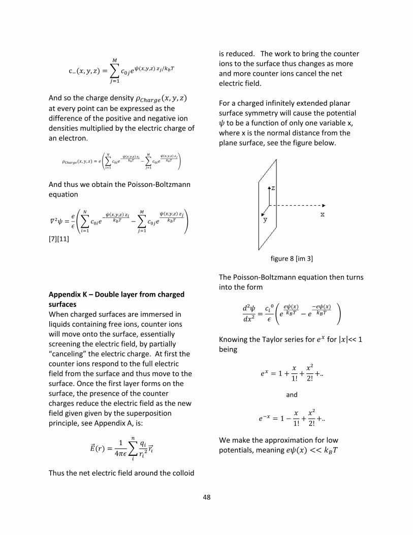
48
c−(𝑥, 𝑦, 𝑧) =∑𝑐0𝑗𝑒𝜓(𝑥,𝑦,𝑧) 𝑧𝑗/𝑘𝑏𝑇
𝑀
𝑗=1
And so the charge density 𝜌𝐶ℎ𝑎𝑟𝑔𝑒(𝑥, 𝑦, 𝑧)
at every point can be expressed as the difference of the positive and negative ion densities multiplied by the electric charge of an electron.
𝜌𝐶ℎ𝑎𝑟𝑔𝑒(𝑥, 𝑦, 𝑧) = 𝑒 (∑𝑐0𝑖𝑒−𝜓(𝑥,𝑦,𝑧) 𝑧𝑖
𝑘𝑏𝑇
𝑁
𝑖=1
−∑𝑐0𝑖𝑒𝜓(𝑥,𝑦,𝑧) 𝑧𝑗
𝑘𝑏𝑇
𝑀
𝑗=1
)
And thus we obtain the Poisson-Boltzmann equation
𝛻2𝜓 =𝑒
𝜖(∑𝑐0𝑖𝑒
−𝜓(𝑥,𝑦,𝑧) 𝑧𝑖
𝑘𝑏𝑇
𝑁
𝑖=1
−∑𝑐0𝑗𝑒𝜓(𝑥,𝑦,𝑧) 𝑧𝑗
𝑘𝑏𝑇
𝑀
𝑗=1
)
[7][11]
Appendix K – Double layer from charged surfaces When charged surfaces are immersed in liquids containing free ions, counter ions will move onto the surface, essentially screening the electric field, by partially “canceling” the electric charge. At first the counter ions respond to the full electric field from the surface and thus move to the surface. Once the first layer forms on the surface, the presence of the counter charges reduce the electric field as the new field given given by the superposition principle, see Appendix A, is:
�⃗⃗�(𝑟) =1
4𝜋𝜖∑
𝑞𝑖𝑟𝑖²𝑟𝑖⃗⃗⃗
𝑛
𝑖
Thus the net electric field around the colloid
is reduced. The work to bring the counter ions to the surface thus changes as more and more counter ions cancel the net electric field. For a charged infinitely extended planar surface symmetry will cause the potential 𝜓 to be a function of only one variable x, where x is the normal distance from the plane surface, see the figure below.
figure 8 [im 3]
The Poisson-Boltzmann equation then turns into the form
𝑑²𝜓
𝑑𝑥²=𝑐𝑖⁰
𝜖(𝑒
𝑒𝜓(𝑥)𝑘𝐵𝑇 − 𝑒
−𝑒𝜓(𝑥)𝑘𝐵𝑇 )
Knowing the Taylor series for 𝑒𝑥 for |𝑥|<< 1 being
𝑒𝑥 = 1 +𝑥
1!+𝑥²
2!+..
and
𝑒−𝑥 = 1 −𝑥
1!+𝑥²
2!+..
We make the approximation for low potentials, meaning 𝑒𝜓(𝑥) << 𝑘𝐵𝑇
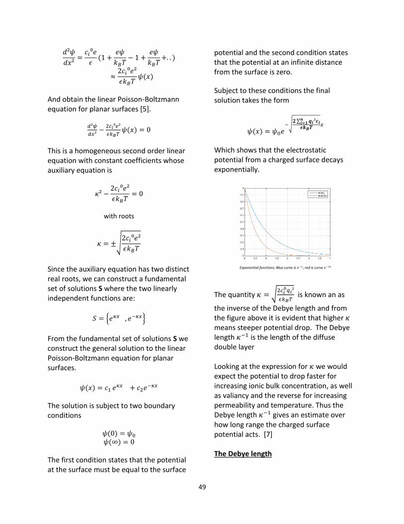
49
𝑑²𝜓
𝑑𝑥²=𝑐𝑖⁰𝑒
𝜖(1 +
𝑒𝜓
𝑘𝐵𝑇− 1 +
𝑒𝜓
𝑘𝐵𝑇+. . )
≈2𝑐𝑖⁰𝑒²
𝜖𝑘𝐵𝑇𝜓(𝑥)
And obtain the linear Poisson-Boltzmann equation for planar surfaces [5].
𝑑²𝜓
𝑑𝑥²−2𝑐𝑖⁰𝑒²
𝜖𝑘𝐵𝑇𝜓(𝑥) = 0
This is a homogeneous second order linear equation with constant coefficients whose auxiliary equation is
𝜅² −2𝑐𝑖⁰𝑒²
𝜖𝑘𝐵𝑇= 0
with roots
𝜅 = ±√2𝑐𝑖⁰𝑒²
𝜖𝑘𝐵𝑇
Since the auxiliary equation has two distinct real roots, we can construct a fundamental set of solutions S where the two linearly independent functions are:
𝑆 = {𝑒𝜅𝑥 , 𝑒−𝜅𝑥}
From the fundamental set of solutions S we construct the general solution to the linear Poisson-Boltzmann equation for planar surfaces.
𝜓(𝑥) = 𝑐1 𝑒𝜅𝑥 + 𝑐2𝑒
−𝜅𝑥
The solution is subject to two boundary conditions
𝜓(0) = 𝜓0 𝜓(∞) = 0
The first condition states that the potential at the surface must be equal to the surface
potential and the second condition states that the potential at an infinite distance from the surface is zero.
Subject to these conditions the final solution takes the form
𝜓(𝑥) = 𝜓0𝑒−√
𝟐∑ 𝒒𝒊²𝒏𝒊=𝟏 𝒄𝒊𝝐𝒌𝑩𝑻
𝑥
Which shows that the electrostatic potential from a charged surface decays exponentially.
Exponential functions: Blue curve is 𝑒−𝑥, red is curve 𝑒−2𝑥
The quantity 𝜅 = √2𝑐𝑖
0𝑞𝑖²
𝜖𝑘𝐵𝑇 is known an as
the inverse of the Debye length and from the figure above it is evident that higher 𝜅 means steeper potential drop. The Debye length 𝜅−1 is the length of the diffuse double layer Looking at the expression for 𝜅 we would expect the potential to drop faster for increasing ionic bulk concentration, as well as valiancy and the reverse for increasing permeability and temperature. Thus the Debye length 𝜅−1 gives an estimate over how long range the charged surface potential acts. [7] The Debye length
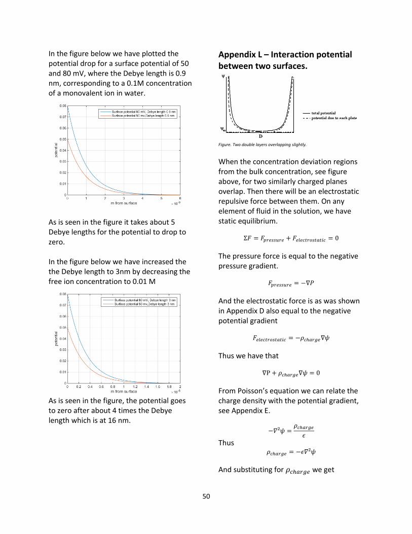
50
In the figure below we have plotted the potential drop for a surface potential of 50 and 80 mV, where the Debye length is 0.9 nm, corresponding to a 0.1M concentration of a monovalent ion in water.
As is seen in the figure it takes about 5 Debye lengths for the potential to drop to zero. In the figure below we have increased the the Debye length to 3nm by decreasing the free ion concentration to 0.01 M
As is seen in the figure, the potential goes to zero after about 4 times the Debye length which is at 16 nm.
Appendix L – Interaction potential between two surfaces.
Figure. Two double layers overlapping slightly.
When the concentration deviation regions from the bulk concentration, see figure above, for two similarly charged planes overlap. Then there will be an electrostatic repulsive force between them. On any element of fluid in the solution, we have static equilibrium.
Σ𝐹 = 𝐹𝑝𝑟𝑒𝑠𝑠𝑢𝑟𝑒 + 𝐹𝑒𝑙𝑒𝑐𝑡𝑟𝑜𝑠𝑡𝑎𝑡𝑖𝑐 = 0
The pressure force is equal to the negative pressure gradient.
𝐹𝑝𝑟𝑒𝑠𝑠𝑢𝑟𝑒 = −∇𝑃
And the electrostatic force is as was shown in Appendix D also equal to the negative potential gradient
𝐹𝑒𝑙𝑒𝑐𝑡𝑟𝑜𝑠𝑡𝑎𝑡𝑖𝑐 = −𝜌𝑐ℎ𝑎𝑟𝑔𝑒∇𝜓
Thus we have that
∇P + 𝜌𝑐ℎ𝑎𝑟𝑔𝑒∇𝜓 = 0
From Poisson’s equation we can relate the charge density with the potential gradient, see Appendix E.
−𝛻²𝜓 =𝜌𝑐ℎ𝑎𝑟𝑔𝑒
𝜖
Thus 𝜌𝑐ℎ𝑎𝑟𝑔𝑒 = −𝜖𝛻²𝜓
And substituting for 𝜌𝑐ℎ𝑎𝑟𝑔𝑒 we get
51
∇P − 𝜖𝛻²𝜓∇𝜓 = 0
Taking 𝑑𝜓
𝑑𝑥 as a variable we notice the
following 𝑑
𝑑𝑥(𝑑𝜓
𝑑𝑥)2
= 2(𝑑𝜓
𝑑𝑥)(𝑑2𝜓
𝑑𝑥2)
That is that the derivative of the first derivative
of 𝜓 squared 𝑑
𝑑𝑥(𝑑𝜓
𝑑𝑥)2 is equal to two times the
derivative 2𝑑𝜓
𝑑𝑥 multiplied by the inner
derivative which is 𝑑2𝜓
𝑑𝑥2. We solve for
(𝑑𝜓
𝑑𝑥) (
𝑑2𝜓
𝑑𝑥2)
And get that
(𝑑𝜓
𝑑𝑥) (𝑑2𝜓
𝑑𝑥2) =
1
2
𝑑
𝑑𝑥(𝑑𝜓
𝑑𝑥)2
So
∇P −𝜖
2
𝑑
𝑑𝑥(𝑑𝜓
𝑑𝑥)
2
= 0
We then factor our 𝑑
𝑑𝑥 and get that
𝑑
𝑑𝑥(P −
𝜖
2(𝑑𝜓
𝑑𝑥)2
) = 0
Where P is the pressure due to the counter
ions accumulating in the gap and −𝜖
2(𝑑𝜓
𝑑𝑥)2
is known as the Maxwell stress term, and represents the repulsion due to the electric field from the surface potential, recall from Appendix C, that
�⃗⃗� = −∇𝜓 = −𝑑𝜓
𝑑𝑥
Taking the derivative with respect to the radial distance, we see that. And thus we conclude that the total pressure force is constant everywhere in the gap. In the middle between the planes, due to
symmetry, the electric fields from both planes cancel, and thus the Maxwell stress term, is zero.
�⃗⃗� (𝑑
2) = −
𝑑𝜓
𝑑𝑥|𝑥=𝑑2
= 0
So that the total force is only dependent on the pressure.
Σ𝐹 (𝑑
2) = 𝐹𝑝𝑟𝑒𝑠𝑠𝑢𝑟𝑒 (
𝑑
2)
To get an expression for the pressure gradient ∇P we use the Poisson-Boltzmann equation
𝑑2𝜓
𝑑𝑥2=𝑒
𝜖(𝑐0𝑒−𝜓(𝑥) 𝑞𝑘𝑏𝑇 − 𝑐0𝑒
𝜓(𝑥)q𝑘𝑏𝑇 )
Noting that the hyperbolic function of sine is
𝑠𝑖𝑛ℎ(𝑥) =𝑒𝑥 − 𝑒−𝑥
2
We rewrite 𝜌𝐶ℎ𝑎𝑟𝑔𝑒 as
𝜌(𝑥) = −2𝑒𝑐0(𝑒𝜓(𝑥)𝑞𝑘𝑏𝑇 − 𝑒
−𝜓(𝑥,)q𝑘𝑏𝑇
2)
𝜌(𝑥) = −2𝑒𝑐0𝑠𝑖𝑛ℎ (𝜓(𝑥)𝑞
𝑘𝐵𝑇)
−2𝑒𝑐0∫𝑠𝑖𝑛ℎ (𝜓(𝑥)𝑞
𝑘𝐵𝑇) 𝑑𝑥 = −2𝑒𝑐0 cosh(
𝜓(𝑥)𝑞
𝑘𝐵𝑇) + 𝐶
Using the relation
cosh(𝑥) =𝑒𝑥 + 𝑒−𝑥
2
We get
−2𝑒𝑐0 (𝑒𝜓(𝑥)𝑞𝑘𝐵𝑇 + 𝑒
−𝜓(𝑥)𝑞𝑘𝐵𝑇
2)
52
And thus we obtain
𝑒𝑐0 (𝑒−𝜓(𝑥) 𝑞
𝑘𝑏𝑇 + 𝑒
𝜓(𝑥) 𝑞
𝑘𝑏𝑇 ) −𝜖
2
𝑑
𝑑𝑥(𝑑𝜓
𝑑𝑥)2
= 0
Comparing this equation with
∇P −𝜖
2
𝑑
𝑑𝑥(𝑑𝜓
𝑑𝑥)
2
= 0
We conclude that
∇𝑃 = 𝑒𝑐0 (𝑒−𝜓(𝑥) 𝑞
𝑘𝑏𝑇 + 𝑒
𝜓(𝑥) 𝑞
𝑘𝑏𝑇 )
To get the pressure between the plates, we remove the osmotic pressure gradient from the pressure gradient ∇𝑃.
∇𝑃𝑜𝑠𝑚𝑜𝑡𝑖𝑐 = 2𝑘𝐵𝑇𝑐0
And conclude that the pressure force acting on the planes, and all the ions in the gap between them is given by the expression
𝐹(𝑥)𝑝𝑟𝑒𝑠𝑠𝑢𝑟𝑒 = ∇𝑃 − ∇𝑃𝑜𝑠𝑚𝑜𝑡𝑖𝑐
𝐹(𝑥)𝑝𝑟𝑒𝑠𝑠𝑢𝑟𝑒 = 𝑐0𝑘𝐵𝑇 (𝑒−𝜓(𝑥) 𝑞
𝑘𝑏𝑇 + 𝑒
𝜓(𝑥) 𝑞
𝑘𝑏𝑇 − 2)
To get the total force acting between the plates we expand the pressure force at the middle in a Taylor series, see Appendix G:
𝐹 (𝑑
2) = 𝑘𝑏𝑇𝑐0
(
1 +
𝑒𝜓(𝑑2)
𝑘𝐵𝑇+1
2!
(
𝑒𝜓(𝑑
2)
𝑘𝐵𝑇
)
2
+⋯
+
(
1 −
𝑒𝜓(𝑑2)
𝑘𝐵𝑇+1
2!
(
𝑒𝜓 (
𝑑2)
𝑘𝐵𝑇
)
+⋯2
)
)
Neglecting the terms higher than the quadratic we obtain the force between the
planes as
𝐹 (𝑑
2) ≈ 𝑘𝑏𝑇𝑐0(
𝑞2𝜓 (𝑑2)2
𝑘𝐵2𝑇2
) =𝑐0𝑞
2𝜓(𝑑2)2
𝑘𝐵𝑇
Using the result from Appendix K at the inverse of the Debye length for a charged planar surface is equal to
𝜅 = √2𝑐𝑖
0𝑞𝑖2
𝜖𝑘𝐵𝑇
We make the substitution
𝜖
2𝜅2 =
𝑐𝑖0𝑞𝑖
2
𝑘𝐵𝑇
And thus the force at the middle of the plane is
𝐹(𝑥) =𝜖
2𝜅2𝜓𝑚𝑖𝑑𝑑𝑙𝑒
2
Since we concluded that the force is the same everywhere in the gap, at equilibrium the force everywhere between the planes is equal to
Σ𝐹(𝑥) =𝜖
2𝜓 (
𝑑
2)2
𝜅2
Assuming the potentials between the planes are additive, that is that their own potential function does not alter in the presence of the other one, and that the double layers overlap only slightly, that is 𝑥 ≫ 𝜅−1we take the potential in the middle to be
ψmiddle = Σ𝜓 = 𝜓𝑃𝑙𝑎𝑛𝑒𝐴 (𝑑
2) + 𝜓𝑃𝑙𝑎𝑛𝑒𝐵 (
𝑑
2)
Due to symmetry
𝜓𝑃𝑙𝑎𝑛𝑒𝐴 (𝑑
2) = 𝜓𝑃𝑙𝑎𝑛𝑒𝐵 (
𝑑
2)
And thus
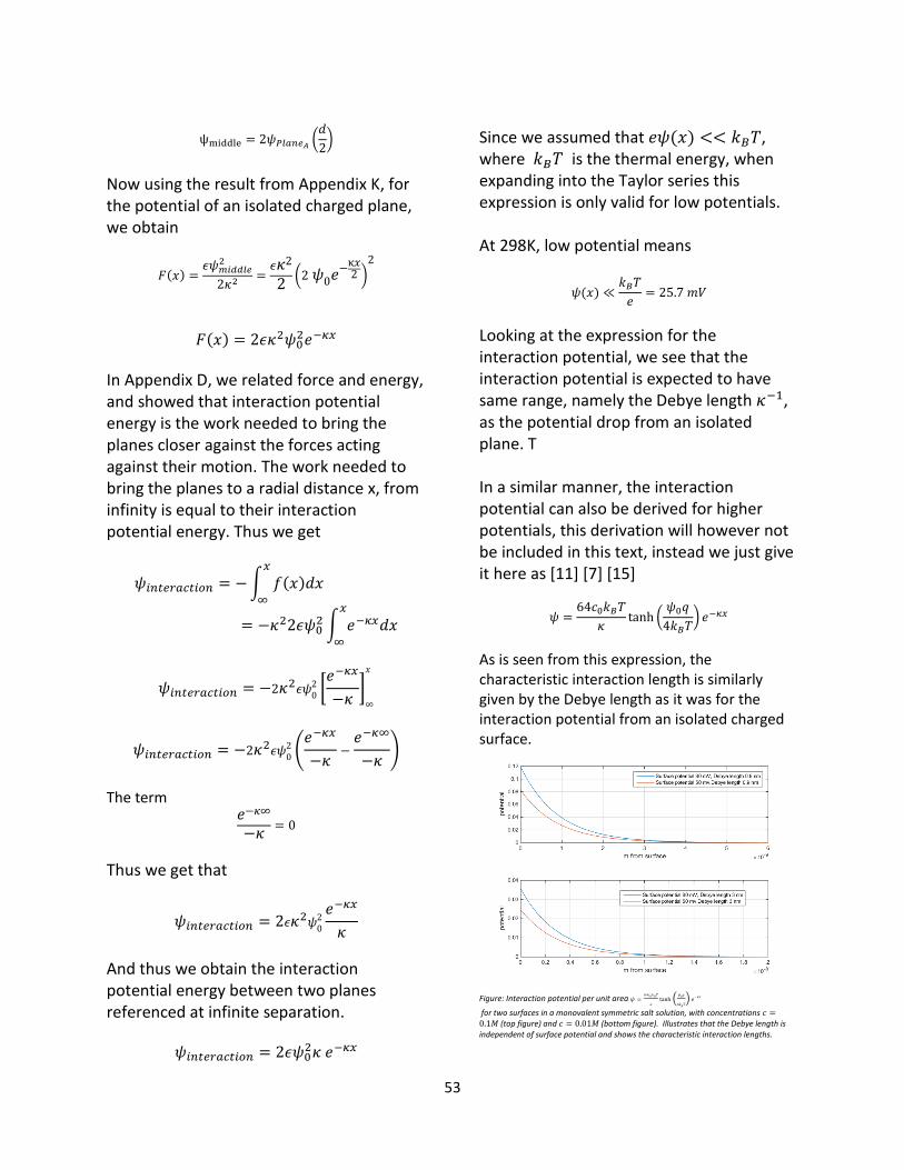
53
ψmiddle = 2𝜓𝑃𝑙𝑎𝑛𝑒𝐴 (𝑑
2)
Now using the result from Appendix K, for the potential of an isolated charged plane, we obtain
𝐹(𝑥) =𝜖𝜓𝑚𝑖𝑑𝑑𝑙𝑒
2
2𝜅2=𝜖𝜅2
2(2 𝜓0𝑒
−κ𝑥2 )
2
𝐹(𝑥) = 2𝜖𝜅2𝜓02𝑒−𝜅𝑥
In Appendix D, we related force and energy, and showed that interaction potential energy is the work needed to bring the planes closer against the forces acting against their motion. The work needed to bring the planes to a radial distance x, from infinity is equal to their interaction potential energy. Thus we get
𝜓𝑖𝑛𝑡𝑒𝑟𝑎𝑐𝑡𝑖𝑜𝑛 = −∫ 𝑓(𝑥)𝑑𝑥𝑥
∞
= −𝜅22𝜖𝜓02∫ 𝑒−𝜅𝑥𝑑𝑥
𝑥
∞
𝜓𝑖𝑛𝑡𝑒𝑟𝑎𝑐𝑡𝑖𝑜𝑛 = −2𝜅2𝜖𝜓
02 [𝑒−𝜅𝑥
−𝜅]∞
𝑥
𝜓𝑖𝑛𝑡𝑒𝑟𝑎𝑐𝑡𝑖𝑜𝑛 = −2𝜅2𝜖𝜓
02 (𝑒−𝜅𝑥
−𝜅−𝑒−𝜅∞
−𝜅)
The term 𝑒−𝜅∞
−𝜅= 0
Thus we get that
𝜓𝑖𝑛𝑡𝑒𝑟𝑎𝑐𝑡𝑖𝑜𝑛 = 2𝜖𝜅2𝜓
02𝑒−𝜅𝑥
𝜅
And thus we obtain the interaction potential energy between two planes referenced at infinite separation.
𝜓𝑖𝑛𝑡𝑒𝑟𝑎𝑐𝑡𝑖𝑜𝑛 = 2𝜖𝜓0
2𝜅 𝑒−𝜅𝑥
Since we assumed that 𝑒𝜓(𝑥) << 𝑘𝐵𝑇, where 𝑘𝐵𝑇 is the thermal energy, when expanding into the Taylor series this expression is only valid for low potentials. At 298K, low potential means
𝜓(𝑥) ≪𝑘𝐵𝑇
𝑒= 25.7 𝑚𝑉
Looking at the expression for the interaction potential, we see that the interaction potential is expected to have same range, namely the Debye length 𝜅−1, as the potential drop from an isolated plane. T In a similar manner, the interaction potential can also be derived for higher potentials, this derivation will however not be included in this text, instead we just give it here as [11] [7] [15]
𝜓 =64𝑐0𝑘𝐵𝑇
𝜅tanh (
𝜓0𝑞
4𝑘𝐵𝑇) 𝑒−𝜅𝑥
As is seen from this expression, the characteristic interaction length is similarly given by the Debye length as it was for the interaction potential from an isolated charged surface.
Figure: Interaction potential per unit area 𝜓 =
64𝑐0𝑘𝐵𝑇
𝜅tanh (
𝜓0𝑞
4𝑘𝐵𝑇) 𝑒−𝜅𝑥
for two surfaces in a monovalent symmetric salt solution, with concentrations 𝑐 =0.1𝑀 (top figure) and 𝑐 = 0.01𝑀 (bottom figure). Illustrates that the Debye length is independent of surface potential and shows the characteristic interaction lengths.
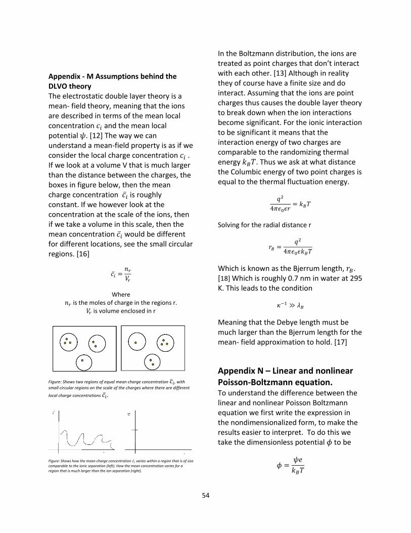
54
Appendix - M Assumptions behind the DLVO theory The electrostatic double layer theory is a mean- field theory, meaning that the ions are described in terms of the mean local concentration 𝑐𝑖 and the mean local potential 𝜓. [12] The way we can understand a mean-field property is as if we consider the local charge concentration 𝑐𝑖 . If we look at a volume V that is much larger than the distance between the charges, the boxes in figure below, then the mean charge concentration 𝑐�̅� is roughly constant. If we however look at the concentration at the scale of the ions, then if we take a volume in this scale, then the mean concentration 𝑐�̅� would be different for different locations, see the small circular regions. [16]
𝑐�̅� =𝑛𝑟𝑉𝑟
Where
𝑛𝑟 is the moles of charge in the regions r. 𝑉𝑟 is volume enclosed in r
Figure: Shows two regions of equal mean charge concentration �̅�𝑖, with
small circular regions on the scale of the charges where there are different
local charge concentrations 𝑐�̅�.
Figure: Shows how the mean charge concentration 𝑐�̅� varies within a region that is of size comparable to the ionic separation (left). How the mean concentration varies for a region that is much larger than the ion separation (right).
In the Boltzmann distribution, the ions are treated as point charges that don’t interact with each other. [13] Although in reality they of course have a finite size and do interact. Assuming that the ions are point charges thus causes the double layer theory to break down when the ion interactions become significant. For the ionic interaction to be significant it means that the interaction energy of two charges are comparable to the randomizing thermal energy 𝑘𝐵𝑇. Thus we ask at what distance the Columbic energy of two point charges is equal to the thermal fluctuation energy.
𝑞2
4𝜋𝜖0𝜖𝑟= 𝑘𝐵𝑇
Solving for the radial distance r
𝑟𝐵 =𝑞2
4𝜋𝜖0𝜖𝑘𝐵𝑇
Which is known as the Bjerrum length, 𝑟𝐵. [18] Which is roughly 0.7 nm in water at 295 K. This leads to the condition
𝜅−1 ≫ 𝜆𝐵
Meaning that the Debye length must be much larger than the Bjerrum length for the mean- field approximation to hold. [17]
Appendix N – Linear and nonlinear Poisson-Boltzmann equation. To understand the difference between the linear and nonlinear Poisson Boltzmann equation we first write the expression in the nondimensionalized form, to make the results easier to interpret. To do this we take the dimensionless potential 𝜙 to be
𝜙 =𝜓𝑒
𝑘𝐵𝑇
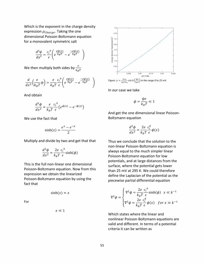
55
Which is the exponent in the charge density expression 𝜌𝐶ℎ𝑎𝑟𝑔𝑒. Taking the one
dimensional Poisson-Boltzmann equation for a monovalent symmetric salt
𝑑²𝜓
𝑑𝑥²=𝑐𝑖⁰
𝜖(𝑒
𝑒𝜓(𝑥)𝑘𝐵𝑇 − 𝑒
−𝑒𝜓(𝑥)𝑘𝐵𝑇 )
We then multiply both sides by 𝑒
𝑘𝐵𝑇
𝑑
𝑑𝑥2(𝑒
𝑘𝐵𝑇𝜓) =
𝑒
𝑘𝐵𝑇
𝑐𝑖⁰
𝜖(𝑒
𝑒𝜓(𝑥)𝑘𝐵𝑇 − 𝑒
−𝑒𝜓(𝑥)𝑘𝐵𝑇 )
And obtain
𝑑2𝜙
𝑑𝑥2=
𝑒
𝑘𝐵𝑇
𝑐𝑖⁰
𝜖(𝑒𝜙(𝑥) − e−𝜙(𝑥))
We use the fact that
sinh(𝑥) =𝑒𝑥 − 𝑒−𝑥
2
Multiply and divide by two and get that that
𝑑2𝜙
𝑑𝑥2=2𝑒
𝑘𝐵𝑇
𝑐𝑖⁰
𝜖sinh(𝜙)
This is the full non-linear one dimensional Poisson-Boltzmann equation. Now from this expression we obtain the linearized Poisson-Boltzmann equation by using the fact that
sinh (𝑥) ≈ 𝑥 For
𝑥 ≪ 1
Figure: 𝑦 =
2𝑒𝑐0
𝑘𝐵𝑇𝜖𝜖0𝑠𝑖𝑛 ℎ (
𝜓𝑞
𝑘𝐵𝑇) in the range 0 to 25 mV.
In our case we take
𝜙 =𝜓𝑒
𝑘𝐵𝑇≪ 1
And get the one dimensional linear Poisson-Boltzmann equation
𝑑2𝜙
𝑑𝑥2=2𝑒
𝑘𝐵𝑇
𝑐𝑖0
𝜖𝜙(𝑥)
Thus we conclude that the solution to the non-linear Poisson-Boltzmann equation is always equal to the much simpler linear Poisson-Boltzmann equation for low potentials, and at large distances from the surface, where the potential gets lower than 25 mV at 295 K. We could therefore define the Laplacian of the potential as the piecewise partial differential equation
∇2𝜙 =
{
∇2𝜙 =
2𝑒
𝑘𝐵𝑇
𝑐𝑖⁰
𝜖sinh(𝜙) 𝑥 ≪ 𝑘−1
∇2𝜙 =2𝑒
𝑘𝐵𝑇
𝑐𝑖0
𝜖𝜙(𝑥) 𝑓𝑜𝑟 𝑥 ≫ 𝑘−1
Which states where the linear and nonlinear Poisson-Boltzmann equations are valid and different. In terms of a potential criteria it can be written as
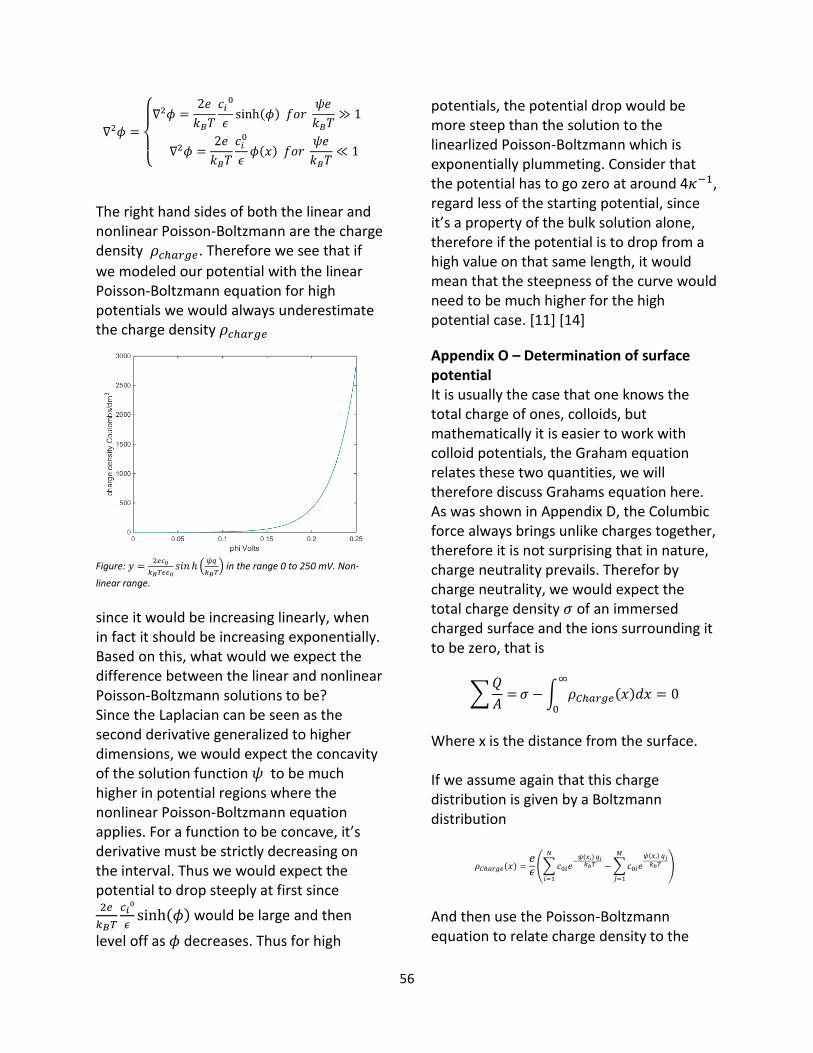
56
∇2𝜙 =
{
∇2𝜙 =
2𝑒
𝑘𝐵𝑇
𝑐𝑖⁰
𝜖sinh(𝜙) 𝑓𝑜𝑟
𝜓𝑒
𝑘𝐵𝑇≫ 1
∇2𝜙 =2𝑒
𝑘𝐵𝑇
𝑐𝑖0
𝜖𝜙(𝑥) 𝑓𝑜𝑟
𝜓𝑒
𝑘𝐵𝑇≪ 1
The right hand sides of both the linear and nonlinear Poisson-Boltzmann are the charge density 𝜌𝑐ℎ𝑎𝑟𝑔𝑒. Therefore we see that if
we modeled our potential with the linear Poisson-Boltzmann equation for high potentials we would always underestimate the charge density 𝜌𝑐ℎ𝑎𝑟𝑔𝑒
Figure: 𝑦 =
2𝑒𝑐0
𝑘𝐵𝑇𝜖𝜖0𝑠𝑖𝑛 ℎ (
𝜓𝑞
𝑘𝐵𝑇) in the range 0 to 250 mV. Non-
linear range.
since it would be increasing linearly, when in fact it should be increasing exponentially. Based on this, what would we expect the difference between the linear and nonlinear Poisson-Boltzmann solutions to be? Since the Laplacian can be seen as the second derivative generalized to higher dimensions, we would expect the concavity of the solution function 𝜓 to be much higher in potential regions where the nonlinear Poisson-Boltzmann equation applies. For a function to be concave, it’s derivative must be strictly decreasing on the interval. Thus we would expect the potential to drop steeply at first since 2𝑒
𝑘𝐵𝑇
𝑐𝑖⁰
𝜖sinh(𝜙) would be large and then
level off as 𝜙 decreases. Thus for high
potentials, the potential drop would be more steep than the solution to the linearlized Poisson-Boltzmann which is exponentially plummeting. Consider that the potential has to go zero at around 4𝜅−1, regard less of the starting potential, since it’s a property of the bulk solution alone, therefore if the potential is to drop from a high value on that same length, it would mean that the steepness of the curve would need to be much higher for the high potential case. [11] [14]
Appendix O – Determination of surface potential It is usually the case that one knows the total charge of ones, colloids, but mathematically it is easier to work with colloid potentials, the Graham equation relates these two quantities, we will therefore discuss Grahams equation here. As was shown in Appendix D, the Columbic force always brings unlike charges together, therefore it is not surprising that in nature, charge neutrality prevails. Therefor by charge neutrality, we would expect the total charge density 𝜎 of an immersed charged surface and the ions surrounding it to be zero, that is
∑𝑄
𝐴=𝜎 −∫ 𝜌𝐶ℎ𝑎𝑟𝑔𝑒(𝑥)𝑑𝑥 = 0
∞
0
Where x is the distance from the surface. If we assume again that this charge distribution is given by a Boltzmann distribution
𝜌𝐶ℎ𝑎𝑟𝑔𝑒(𝑥) =𝑒𝜖(∑𝑐0𝑖𝑒
−𝜓(𝑥,) 𝑞𝑖𝑘𝑏𝑇
𝑁
𝑖=1
−∑𝑐0𝑖𝑒𝜓(𝑥,) 𝑞𝑗𝑘𝑏𝑇
𝑀
𝑗=1
)
And then use the Poisson-Boltzmann equation to relate charge density to the
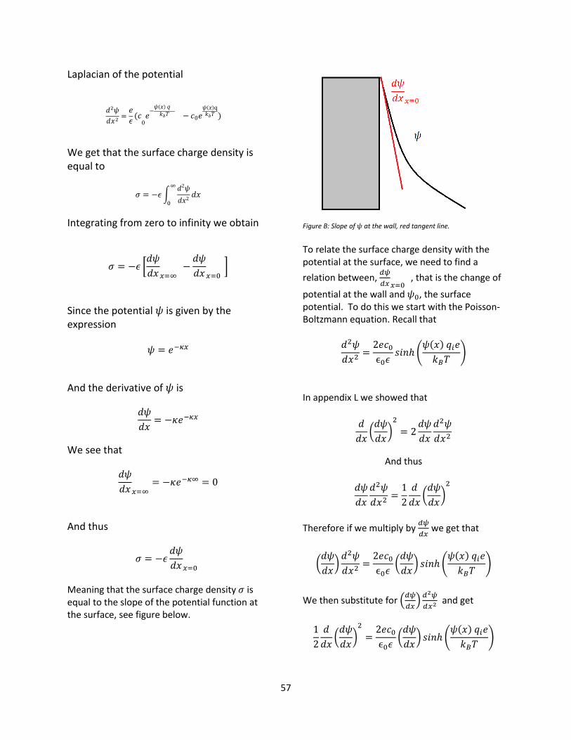
57
Laplacian of the potential
𝑑2𝜓
𝑑𝑥2=𝑒
𝜖(𝑐0𝑒−𝜓(𝑥) 𝑞𝑘𝑏𝑇 − 𝑐0𝑒
𝜓(𝑥)q𝑘𝑏𝑇 )
We get that the surface charge density is equal to
𝜎 = −𝜖∫𝑑2𝜓
𝑑𝑥2
∞
0
𝑑𝑥
Integrating from zero to infinity we obtain
𝜎 = −𝜖 [𝑑𝜓
𝑑𝑥𝑥=∞ −𝑑𝜓
𝑑𝑥𝑥=0 ]
Since the potential 𝜓 is given by the expression
𝜓 = 𝑒−𝜅𝑥
And the derivative of 𝜓 is
𝑑𝜓
𝑑𝑥= −𝜅𝑒−𝜅𝑥
We see that
𝑑𝜓
𝑑𝑥𝑥=∞= −𝜅𝑒−𝜅∞ = 0
And thus
𝜎 = −𝜖𝑑𝜓
𝑑𝑥𝑥=0
Meaning that the surface charge density 𝜎 is equal to the slope of the potential function at the surface, see figure below.
Figure B: Slope of 𝜓 at the wall, red tangent line.
To relate the surface charge density with the potential at the surface, we need to find a
relation between, 𝑑𝜓
𝑑𝑥𝑥=0 , that is the change of
potential at the wall and 𝜓0, the surface potential. To do this we start with the Poisson-Boltzmann equation. Recall that
𝑑2𝜓
𝑑𝑥2=2𝑒𝑐0ϵ0𝜖
𝑠𝑖𝑛ℎ (𝜓(𝑥) 𝑞𝑖𝑒
𝑘𝐵𝑇)
In appendix L we showed that
𝑑
𝑑𝑥(𝑑𝜓
𝑑𝑥)2
= 2𝑑𝜓
𝑑𝑥
𝑑2𝜓
𝑑𝑥2
And thus
𝑑𝜓
𝑑𝑥
𝑑2𝜓
𝑑𝑥2=1
2
𝑑
𝑑𝑥(𝑑𝜓
𝑑𝑥)2
Therefore if we multiply by 𝑑𝜓
𝑑𝑥 we get that
(𝑑𝜓
𝑑𝑥)𝑑2𝜓
𝑑𝑥2=2𝑒𝑐0ϵ0𝜖
(𝑑𝜓
𝑑𝑥) 𝑠𝑖𝑛ℎ (
𝜓(𝑥) 𝑞𝑖𝑒
𝑘𝐵𝑇)
We then substitute for (𝑑𝜓
𝑑𝑥)𝑑2𝜓
𝑑𝑥2 and get
1
2
𝑑
𝑑𝑥(𝑑𝜓
𝑑𝑥)2
=2𝑒𝑐0ϵ0𝜖
(𝑑𝜓
𝑑𝑥) 𝑠𝑖𝑛ℎ (
𝜓(𝑥) 𝑞𝑖𝑒
𝑘𝐵𝑇)
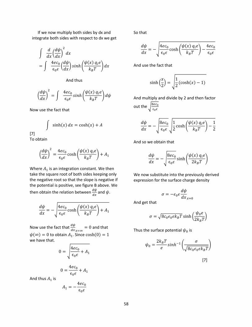
58
If we now multiply both sides by dx and integrate both sides with respect to dx we get
∫𝑑
𝑑𝑥(𝑑𝜓
𝑑𝑥)2
𝑑𝑥
= ∫4𝑒𝑐0ϵ0𝜖
(𝑑𝜓
𝑑𝑥) 𝑠𝑖𝑛ℎ (
𝜓(𝑥) 𝑞𝑖𝑒
𝑘𝐵𝑇)𝑑𝑥
And thus
(𝑑𝜓
𝑑𝑥)2
= ∫4𝑒𝑐0ϵ0𝜖
𝑠𝑖𝑛ℎ (𝜓(𝑥) 𝑞𝑖𝑒
𝑘𝐵𝑇)𝑑𝜓
Now use the fact that
∫ sinh(𝑥) 𝑑𝑥 = cosh (𝑥) + 𝐴
[7] To obtain
(𝑑𝜓
𝑑𝑥)2
=4𝑒𝑐0ϵ0𝜖
cosh(𝜓(𝑥) 𝑞𝑖𝑒
𝑘𝐵𝑇) + 𝐴1
Where 𝐴1 is an integration constant. We then take the square root of both sides keeping only the negative root so that the slope is negative if the potential is positive, see figure B above. We
then obtain the relation between 𝑑𝜓
𝑑𝑥 and 𝜓.
𝑑𝜓
𝑑𝑥= −√
4𝑒𝑐0ϵ0𝜖
cosh(𝜓(𝑥) 𝑞𝑖𝑒
𝑘𝐵𝑇) + 𝐴1
Now use the fact that 𝑑𝜓
𝑑𝑥𝑥=∞= 0 and that
𝜓(∞) = 0 to obtain 𝐴1. Since cosh(0) = 1 we have that.
0 = √4𝑒𝑐0ϵ0𝜖
+ 𝐴1
0 =4𝑒𝑐0ϵ0𝜖
+ 𝐴1
And thus 𝐴1 is
𝐴1 = −4𝑒𝑐0ϵ0𝜖
So that
𝑑𝜓
𝑑𝑥= −√
4𝑒𝑐0ϵ0𝜖
cosh(𝜓(𝑥) 𝑞𝑖𝑒
𝑘𝐵𝑇) −
4𝑒𝑐0ϵ0𝜖
And use the fact that
sinh (𝑥
2) = √
1
2(cosh(𝑥) − 1)
And multiply and divide by 2 and then factor
out the √8𝑒𝑐0
ϵ0𝜖
𝑑𝜓
𝑑𝑥= −√
8𝑒𝑐0ϵ0𝜖
√1
2cosh(
𝜓(𝑥) 𝑞𝑖𝑒
𝑘𝐵𝑇) −
1
2
And so we obtain that
𝑑𝜓
𝑑𝑥= −√
8𝑒𝑐0ϵ0𝜖
sinh(𝜓(𝑥) 𝑞𝑖𝑒
2𝑘𝐵𝑇)
We now substitute into the previously derived expression for the surface charge density
𝜎 = −𝜖0𝜖𝑑𝜓
𝑑𝑥𝑥=0
And get that
𝜎 = √8𝑐0𝜖0𝜖𝑘𝐵𝑇 sinh (𝜓0𝑒
2𝑘𝐵𝑇)
Thus the surface potential 𝜓0 is
𝜓0 =2𝑘𝐵𝑇
𝑒𝑠𝑖𝑛ℎ−1 (
𝜎
√8𝑐0𝜖0𝜖𝑘𝐵𝑇)
[7]
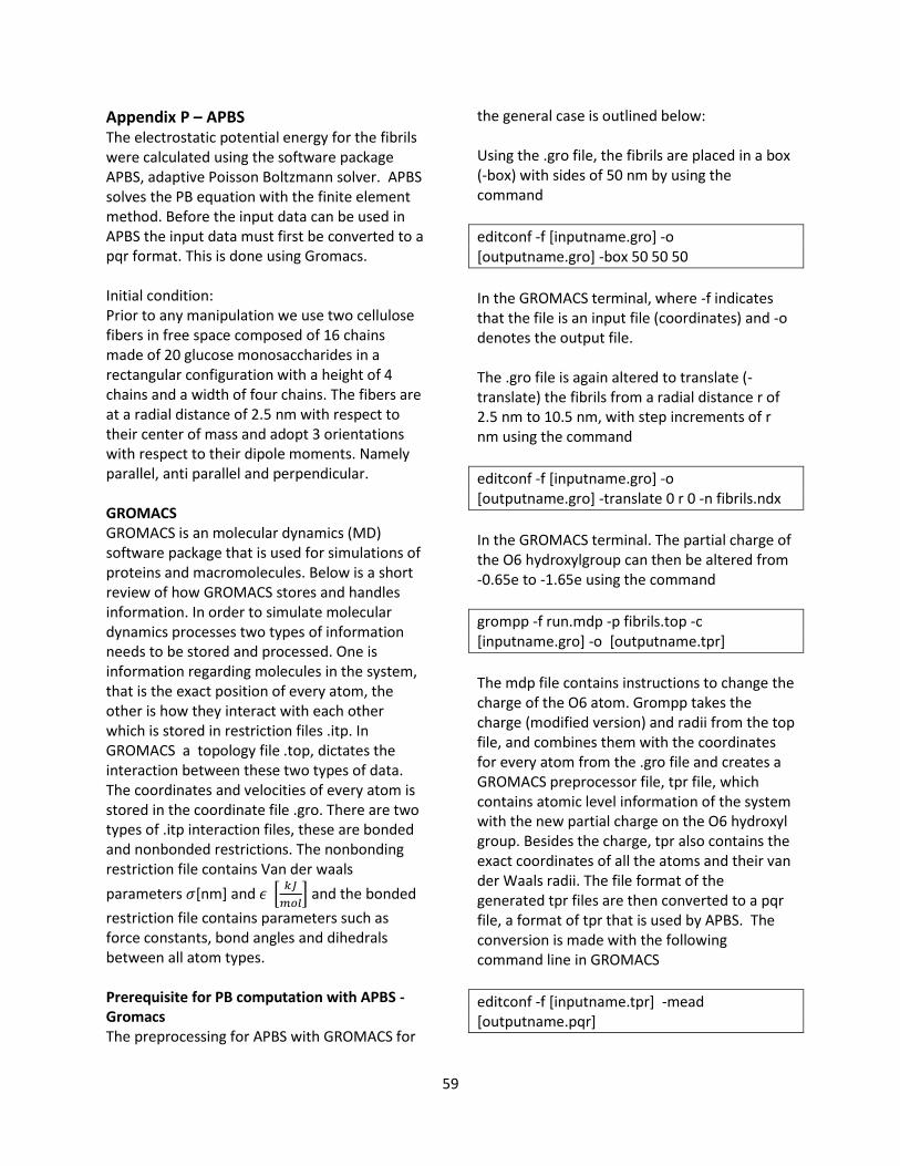
59
Appendix P – APBS The electrostatic potential energy for the fibrils were calculated using the software package APBS, adaptive Poisson Boltzmann solver. APBS solves the PB equation with the finite element method. Before the input data can be used in APBS the input data must first be converted to a pqr format. This is done using Gromacs. Initial condition: Prior to any manipulation we use two cellulose fibers in free space composed of 16 chains made of 20 glucose monosaccharides in a rectangular configuration with a height of 4 chains and a width of four chains. The fibers are at a radial distance of 2.5 nm with respect to their center of mass and adopt 3 orientations with respect to their dipole moments. Namely parallel, anti parallel and perpendicular. GROMACS GROMACS is an molecular dynamics (MD) software package that is used for simulations of proteins and macromolecules. Below is a short review of how GROMACS stores and handles information. In order to simulate molecular dynamics processes two types of information needs to be stored and processed. One is information regarding molecules in the system, that is the exact position of every atom, the other is how they interact with each other which is stored in restriction files .itp. In GROMACS a topology file .top, dictates the interaction between these two types of data. The coordinates and velocities of every atom is stored in the coordinate file .gro. There are two types of .itp interaction files, these are bonded and nonbonded restrictions. The nonbonding restriction file contains Van der waals
parameters 𝜎[nm] and 𝜖 [𝑘𝐽
𝑚𝑜𝑙] and the bonded
restriction file contains parameters such as force constants, bond angles and dihedrals between all atom types. Prerequisite for PB computation with APBS - Gromacs The preprocessing for APBS with GROMACS for
the general case is outlined below: Using the .gro file, the fibrils are placed in a box (-box) with sides of 50 nm by using the command
editconf -f [inputname.gro] -o [outputname.gro] -box 50 50 50
In the GROMACS terminal, where -f indicates that the file is an input file (coordinates) and -o denotes the output file. The .gro file is again altered to translate (-translate) the fibrils from a radial distance r of 2.5 nm to 10.5 nm, with step increments of r nm using the command
editconf -f [inputname.gro] -o [outputname.gro] -translate 0 r 0 -n fibrils.ndx
In the GROMACS terminal. The partial charge of the O6 hydroxylgroup can then be altered from -0.65e to -1.65e using the command
grompp -f run.mdp -p fibrils.top -c [inputname.gro] -o [outputname.tpr]
The mdp file contains instructions to change the charge of the O6 atom. Grompp takes the charge (modified version) and radii from the top file, and combines them with the coordinates for every atom from the .gro file and creates a GROMACS preprocessor file, tpr file, which contains atomic level information of the system with the new partial charge on the O6 hydroxyl group. Besides the charge, tpr also contains the exact coordinates of all the atoms and their van der Waals radii. The file format of the generated tpr files are then converted to a pqr file, a format of tpr that is used by APBS. The conversion is made with the following command line in GROMACS
editconf -f [inputname.tpr] -mead [outputname.pqr]

60
The pqr file contains the exact same information as the tpr file, namely Vander waals radii, atom charges and positions. APBS APBS uses the pqr file with .in files containing calculation parameters to solve the Poisson-Boltzmann equation. Below is an example of an .in file that was used in the calculations:
read pqr mol [name of pqr file].pqr end elec mg-auto dime 385 385 385 cglen 500 500 500 fglen 200 200 200 cgcent mol 1 fgcent mol 1 mol 1 npbe bcfl sdh pdie 1.0000 sdie 78.54 ion charge 1 conc 0.01 radius 2.0 ion charge -1 conc 0.01 radius 2.0 srfm smol chgm spl2 sdens 10.00 srad 1.40 swin 0.30 temp 298.15 calcenergy total end
To start the calculation the pqr file containing the molecular information and the .in file were placed in the same folder and then the following command was simply typed in the terminal
apbs [name of .in file].in
Below is a table stating exactly what each line in
the .in files means.
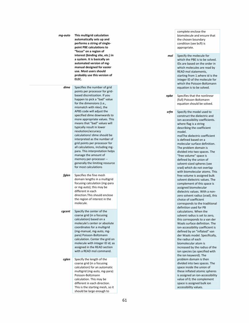
61
mg-auto
This multigrid calculation automatically sets up and performs a string of single-point PBE calculations to “focus” on a region of interest (binding site, etc.) in a system. It is basically an automated version of mg-manual designed for easier use. Most users should probably use this version of ELEC.
dime
Specifies the number of grid points per processor for grid-based discretization. If you happen to pick a "bad" value for the dimensions (i.e., mismatch with nlev), the APBS code will adjust the specified dime downwards to more appropriate values. This means that "bad" values will typically result in lower resolution/accuracy calculations! dime should be interpreted as the number of grid points per processor for all calculations, including mg-para. This interpretation helps manage the amount of memory per-processor -- generally the limiting resource for most calculations
fglen
Specifies the fine mesh domain lengths in a multigrid focusing calculation (mg-para or mg-auto); this may be different in each direction.This should enclose the region of interest in the molecule.
cgcent
Specify the center of the coarse grid (in a focusing calculation) based on a molecule's center or absolute coordinates for a multigrid (mg-manual, mg-auto, mg-para) Poisson-Boltzmann calculation. Center the grid on molecule with integer ID id; as assigned in the READ section with a READ mol command.
cglen
Specify the length of the coarse grid (in a focusing calculation) for an automatic multigrid (mg-auto, mg-para) Poisson-Boltzmann calculation. This may be different in each direction. This is the starting mesh, so it should be large enough to
complete enclose the biomolecule and ensure that the chosen boundary condition (see bcfl) is appropriate.
mol
Specify the molecule for which the PBE is to be solved. IDs are based on the order in which molecules are read by READ mol statements, starting from 1.where id is the integer ID of the molecule for which the Poisson-Boltzmann equation is to be solved.
npbe
Specifies that the nonlinear (full) Poisson-Boltzmann equation should be solved.
srfm
Specify the model used to construct the dielectric and ion-accessibility coefficients. where flag is a string describing the coefficient model. molThe dielectric coefficient is defined based on a molecular surface definition. The problem domain is divided into two spaces. The "free volume" space is defined by the union of solvent-sized spheres (see srad) which do not overlap with biomolecular atoms. This free volume is assigned bulk solvent dielectric values. The complement of this space is assigned biomolecular dielectric values. With a non-zero solvent radius (srad), this choice of coefficient corresponds to the traditional definition used for PB calculations. When the solvent radius is set to zero, this corresponds to a van der Waals surface definition. The ion-accessibility coefficient is defined by an "inflated" van der Waals model. Specifically, the radius of each biomolecular atom is increased by the radius of the ion species (as specified with the ion keyword). The problem domain is then divided into two spaces. The space inside the union of these inflated atomic spheres is assigned an ion-accessibility value of 0; the complement space is assigned bulk ion accessibility values.
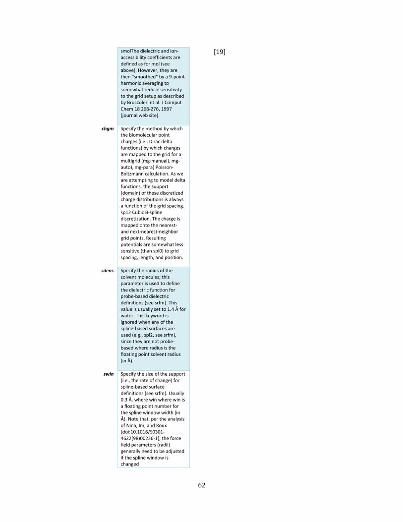
62
smolThe dielectric and ion-accessibility coefficients are defined as for mol (see above). However, they are then "smoothed" by a 9-point harmonic averaging to somewhat reduce sensitivity to the grid setup as described by Bruccoleri et al. J Comput Chem 18 268-276, 1997 (journal web site).
chgm
Specify the method by which the biomolecular point charges (i.e., Dirac delta functions) by which charges are mapped to the grid for a multigrid (mg-manual), mg-auto), mg-para) Poisson-Boltzmann calculation. As we are attempting to model delta functions, the support (domain) of these discretized charge distributions is always a function of the grid spacing. sp12 Cubic B-spline discretization. The charge is mapped onto the nearest- and next-nearest-neighbor grid points. Resulting potentials are somewhat less sensitive (than spl0) to grid spacing, length, and position.
sdens
Specify the radius of the solvent molecules; this parameter is used to define the dielectric function for probe-based dielectric definitions (see srfm). This value is usually set to 1.4 Å for water. This keyword is ignored when any of the spline-based surfaces are used (e.g., spl2, see srfm), since they are not probe-based.where radius is the floating point solvent radius (in Å).
swin
Specify the size of the support (i.e., the rate of change) for spline-based surface definitions (see srfm). Usually 0.3 Å. where win where win is a floating point number for the spline window width (in Å). Note that, per the analysis of Nina, Im, and Roux (doi:10.1016/S0301-4622(98)00236-1), the force field parameters (radii) generally need to be adjusted if the spline window is changed
[19]

63
References
1. E.R. Leite and C. Ribeiro, Crystallization and Growth of Colloidal Nanocrystals, SpringerBriefs in Materials, DOI 10.1007/978-1-4614-1308-0_2, and Caue Ribeiro 2012
2. M ALIN B ERGENSTRÅHLE . Crystalline cellulose in bulk and at interfaces as studied by atomistic computer simulations. Doctoral Thesis Stockholm, Sweden 2008
3. CAREL J. VAN OSS. Interfacial Lifshitz-van der Waals and Polar Interactions in Macroscopic Systems. Departments of Microbloiogy and Chemical Engineering, State University of New York at Buffalo, Buffalo, New York 14214
4. K.S Birdi. Colloid systems and interfaces. Surface and colloid chemistry. p 388-402.
5. Jacob N. Israelachvili . Intermolecular and Surface Forces. Third edition.
6. Michael J. Holst . The Poisson-Boltzmann
Equation Analysis and Multilevel
Numerical Solution, , 1994
7. Hans-Jurgen Butt. Surface and interfacial forces. Electrostatic double layer forces p93-124.
8. Sears, Zemansky University Physics with
Modern Physics (13th) p. 693-695. p709.
p 710. p.320. p711. p755 . p224 p.757.
p732 .p735
9. David Ham. Lecture notes, Finite Element Course. Imperial College London in Autumn 2013/Spring 2014
10. David J. Griffiths - Introduction to
Electrodynamics, Fourth Edition.
11. John Rogawski, Multivariable calculus, 2008 W.H Freeman and Company p.933-1000
12. S.J Farlow, Partial Differential equations for scientists and engineers. p.245
13. http://depts.washington.edu/solgel/page
s/courses/MSE_502/Electrostatic_Stabiliz
ation.html 2015-04-21 10:31
14. Brian J. Kirby, lecture notes, course Mechanical Engineering 6240, Cornell University Nov 28, 2012
15. John Hart, lecture notes, course ME 599: Nanomanufacturing. University of Michigan Oct 26, 2009
16. http://earthweb.ess.washington.edu//Glaciology/courses/ess511/cfr_ch1.pdf 2015-04-21 12:31
17. http://ocw.mit.edu/courses/chemical-
engineering/10-626-electrochemical-
energy-systems-spring-2011/lecture-
notes/MIT10_626S11_lec28.pdf 2015-04-
27 18:26
18. http://ocw.mit.edu/courses/chemical-
engineering/10-626-electrochemical-
energy-systems-spring-2011/lecture-
notes/MIT10_626S11_lec24.pdf 2015-04-
27 21:24
19. http://www.poissonboltzmann.org/docs/apbs-overview/
20. Ken A. Dill, Sarina Bromberg, Molecular driving forces, statistical thermodynamics in Biology, chemistry , physics and Nanoscience. Second Edition. p 318. p.150
21. H.C. Berg, Random Walks in Biology, Princeton (1977)
22. Peter Atkins. Physical Chemistry. Ninth Edition. p.760-770. p.117-118
23. Dr. Prathap Haridoss, lecture notes, Physics of Materials, IIT, Sep 20, 2011.
24. Jan PF Lagerwall. Cellulose nanocrystal-based materials: from liquid crystal self-assembly and glass formation to multifunctional thin films, Fall 2014
25. 26.
References pictures
1. Jacob N. Israelachvili . Intermolecular and Surface Forces. Third edition.
2. http://www.helsinki.fi/polymeerikemia/images/research/cellu_large.jpg 2015-05-11 11:08
3. http://www.tiem.utk.edu/~gross/bioed/webmodules/spherefig2.gif 2015-05-11 18:09
4. http://www.hielscher.com/disperse.htm 2015-05-24
Reference pictures Appendix
1. http://www.wired.com/images_blogs/wire
dscience/2013/08/summer_sketcheskey4.j
pg 11:42 15/03/2015
2. http://upload.wikimedia.org/wikipedia/commons/thumb/3/3e/Dot_Product.svg/2000px-Dot_Product.svg.png 12:00
3. 15/03/2015 4. http://www.mathnotes.org/content/math
/algebra/linear/vectors/images/distance/distance_point_plane_visual.gif 23/03/2015
5. https://www.gearslutz.com/board/attachments/high-end/139979d1255543401-what-flux-density-flux-density.jpg 07/05/2015 10:31
6. http://www.the-idea-shop.com/images/lagrange2.jpg 2015-05-09 16:42
Recommended