INTELLIGENT DECISION SUPPORT SYSTEM FOR USDA FOREST SERVICE
AERIAL SPRAY MANAGEMENT
by
WANYING BI
B.S., Dalian University of Technology, China, 1995
M.S., The University of Pittsburgh, 1998
A Thesis Submitted to the Graduate Faculty
of The University of Georgia in Partial Fulfillment
of the
Requirements for the Degree
MASTER OF SCIENCE
ATHENS, GEORGIA
2000

ii
© 2000
Wanying Bi
All Rights Reserved

iii
INTELLIGENT DECISION SUPPORT SYSTEM FOR USDA FOREST SERVICE
AERIAL SPRAY MANAGEMENT
by
WANYING BI
Approved:
________________________ Major Professor
________________________
Date
Approved:
________________________ Graduate Dean
________________________ Date

iv
ACKNOWLEGEMENTS
I would like to express my sincere gratitude and respect to my advisor, Dr. Walter
Don Potter, for his guidance and helpful instructions during my last two years’ studies at
Athens. I would also like to thank Dr. Ron McClendon and Dr. Chuck Cross for their
supports and being members of my thesis defense committee.
I would like to thank professors and students at the Artificial Intelligence Center
of the University of Georgia for their help and supports. I also thank Angie Paul for her
kind assistance whenever I come to her for help.
I thank my family for their love and concerns, especially my wife, Yu, for her
continuous support and encouragement.

v
TABLE OF CONTENTS
Page
ACKNOWLEDGEMENTS . . . . . . . . . . . . . . . . . . . . . . iv
LIST OF TABLES . . . . . . . . . . . . . . . . . . . . . . . . . . . vii
LIST OF FIGURES . . . . . . . . . . . . . . . . . . . . . . . . . . ix
CHAPTER
1 INTRODUCTION . . . . . . . . . . . . . . . . . . . . . . . . 1
2 BACKGROUND . . . . . . . . . . . . . . . . . . . . . . . . 3
2.1 Forest Spray Prediction . . . . . . . . . . . . . . . . . . . . 3
2.2 Genetic Algorithms . . . . . . . . . . . . . . . . . . . . . . 7
3 DEVELOPMENT OF FORTRAN-SAGA . . . . . . . . . . . . . . . 12
3.1 AGDISP DOS Version 7.0 . . . . . . . . . . . . . . . . . . . 12
3.2 Fortran Simple GA . . . . . . . . . . . . . . . . . . . . . . 13
3.3 Preliminary Fortran-Based SAGA . . . . . . . . . . . . . . . . . 14
3.4 Results and Discussion of Fortran-Based SAGA . . . . . . . . . . . 17
4 DEVELOPMENT OF VB-SAGA1.0 . . . . . . . . . . . . . . . . 23
4.1 VB-SAGA1.0 . . . . . . . . . . . . . . . . . . . . . . . . 23
4.2 Exhaustive Search Test and Comparison with VB-SAGA 1.0 . . . . . . 30
4.3 VB-SAGA1.0 Experiments and Results . . . . . . . . . . . . . . 34
5 DEVELOPMENT OF VB-SAGA2.0 . . . . . . . . . . . . . . . . . 40

vi
5.1 VB-SAGA2.0 Menu Items. . . . . . . . . . . . . . . . . . . . 40
5.2 The Self-Adaptive SAGA. . . . . . . . . . . . . . . . . . . . 42
5.3 Results of VB-SAGA2.0 . . . . . . . . . . . . . . . . . . . . 45
6 SUMMARY AND CONCLUSIONS. . . . . . . . . . . . . . . . . . 48
BIBLIOGRAPHY . . . . . . . . . . . . . . . . . . . . . . . . . . . 51
APPENDIX A . . . . . . . . . . . . . . . . . . . . . . . . . . . . 54
APPENDIX B . . . . . . . . . . . . . . . . . . . . . . . . . . . . .57

vii
LIST OF TABLES
Page
Table 3.1 Fortran-SAGA parameters and their ranges . . . . . . . . . . . . . 16
Table 3.2 An example of preliminary results of Fortran-SAGA . . . . . . . . .17
Table 3.3 Fortran-SAGA results at different population size . . . . . . . . . . 19
Table 3.4 Testing of the Fortran-SAGA parameter importance. . . . . . . . . . 21
Table 4.1 VB-SAGA1.0 spray parameters and their ranges . . . . . . . . . . . 27
Table 4.2 Fixed spray parameters in exhaustive search test . . . . . . . . . . . 31
Table 4.3 Changing spray parameters in exhaustive search test . . . . . . . . . 31
Table 4.4 Fitness results from exhaustive experiment (8 fixed parameters) . . . . . 32
Table 4.5 Fitness results from VB-SAGA 1.0 experiment (8 fixed parameters) . . . 33
Table 4.6 The maximum fitness for exhaustive and VB-SAGA 1.0 tests . . . . . . 33
Table 4.7 The maximum fitness from VB-SAGA1.0 without restrictions on spray
parameters (GA crossover rate=0.65 and mutation rate=0.007) . . . . . .34
Table 4.8 Experiment 1: practical settings with maximum fitness=9710.885. . . . .36
Table 4.9 Experiment 1: practical settings details . . . . . . . . . . . . . . . 36
Table 4.10 Experiment 2: practical settings with maximum fitness=9750.743. . . . 36
Table 4.11 Experiment 2: practical settings details . . . . . . . . . . . . . . .37
Table 4.12 Experiment 3: practical settings details (Aircraft=100 swath width=2.5) . . 37
Table 4.13 Experiment 4: practical settings details (Aircraft=106 swath width=2.25) . .38

viii
Table 4.14 Experiment 5: practical settings details (Aircraft=5 swath width=2.3). . . 38
Table 4.15 Experiment 6: practical settings details (Aircraft=10 swath width=2.2). . 39
Table 5.1 Results from VB-SAGA 1.0 and VB-SAGA 2.0 . . . . . . . . . . . 46
Table 5.2 VB-SAGA 2.0 results for experiment 1 and 2 . . . . . . . . . . . . 46
Table 5.3 VB-SAGA 2.0 results for experiment 3 - 6 . . . . . . . . . . . . . 46

ix
LIST OF FIGURES
Page
Figure 3.1 AGDISP DOS 7.0 main interface when running . . . . . . . . . . . 13
Figure 3.2 Architecture of preliminary Fortran-based SAGA . . . . . . . . . . 15
Figure 3.3 Fortran-SAGA fitness function graph . . . . . . . . . . . . . . . 20
Figure 4.1 Main interface of VB-SAGA1.0 . . . . . . . . . . . . . . . . . 28
Figure 4.2 Main interface of VB-SAGA1.0 with user-specified GA parameters. . . 28
Figure 4.3 Secondary interface of VB-SAGA1.0 to preset spray parameters . . . . 29
Figure 4.4 VB-SAGA1.0 main interface with chart view option turned on . . . . . 29
Figure 4.4 Exhaustive test main interface . . . . . . . . . . . . . . . . . . 31
Figure 5.1 The main interface of VB-SAGA2.0 . . . . . . . . . . . . . . . .41

1
CHAPTER 1
INTRODUCTION
The Intelligent Decision Support System for US Forest Service Spray
Management is a cooperative project between the USDA Forest Service and the Artificial
Intelligence Center at the University of Georgia. The goal of this project is to provide
Forest Service managers a handy tool to predict forest aerial spray performance and
dynamically optimize the spray parameters to save substantial effort, time, and cost in
practical spray tasks.
It has always been a difficult problem to identify ideal spray parameters to
achieve particularly desired deposition, reduce spray material evaporation or drift, and
save the time and money devoted to the spray process [Teske89]. The difficult part of the
problem is that there are dozens of spray parameters in spray practice and each of them
has many possible values. The total combination of possible spray parameters generates
a huge search space (NP hard) that is hardly searchable using traditional techniques
[DeJo89]. For example, 20 parameters each with 20 possible values will lead to a total
combination of 2020 possibilities. It is indeed beyond current computing technology
capacity to find the best solution using approaches such as exhaustive search. In this
project we introduce the Genetic Algorithms to reduce this workload to a large extent by
searching for optimal or near-optimal solutions based on Darwin’s theory of evolution
and survival of the fittest. Our project is named Spray Advisor using Genetic Algorithms

2
(SAGA). This thesis reports the efforts and the achievements of SAGA development as
well as the experimental results and discussion.
Chapter 2 presents detailed background knowledge of aerial spray practice and
simulation, and GA fundamentals and applications. Chapters 3-5 review our
development work of SAGA, each chapter focusing on a version of SAGA at a different
development stage, namely Fortran-SAGA, VB-SAGA1.0, and VB-SAGA2.0. The
experimental results and discussions from these versions are also included. Chapter 6 is a
summary of this project and also some future expectations of this project.

3
CHAPTER 2
BACKGROUND 2.1 Forest Spray Prediction
Aerial spray and pest control has always been an important application in forest
management [Teske89]. Maximum and even deposition, minimum drift and evaporation
loss, and low spraying cost and efforts, are always the main goals for spraying tasks. Of
the many means to facilitate spraying practice, using computer simulation programs has
been the most important and frequently used approach to predict the spray materials
behavior after they are released from the aircraft. These programs construct
mathematical models to dynamically simulate the complicated process when spray
materials are released from the aircraft. A good spray simulation program usually models
the processes such as drift, evaporation, deposition, and dispersion.
The USDA Forest Service has spent abundant time and effort in the past decades
to develop the spray simulation models [Teske93a]. The spray simulation models
simulate the process from the moment the spray material is released from the aircraft
until when they deposit onto the ground. The main models developed for this purpose are
the Forest Service Cramer-Barry-Grim (FSCBG) aerial spray model [Teske89], the
Agricultural Dispersal (AGDISP) model [Teske98a], the Spray Advisor Program, and the
Agricultural Drift (AGDRIFT) model [Teske97], which is a modified version of
AGDISP. We will focus on introducing FSCBG and AGDISP in this chapter.

4
2.1.1 FSCBG Model
FSCBG [Pott99] is designed to model the atmospheric dispersion, transport, and
deposition of all aerial spray materials from the time of release until all spray material is
either deposited or, in the case of spray drift, until the spray concentration and deposition
levels become insignificant. The development of FSCBG was carried out first by the H.
E. Cramer Company and then by Continuum Dynamics, Inc. It includes mathematical
models for aircraft wake effects, gaussian line source dispersion, droplet evaporation,
canopy penetration, ground and canopy deposition. FSCBG predicts the dispersion of the
spray material and the deposition of the material, that is, how much material settles on the
ground and where. FSCBG can be used to optimize the spray program design and assist
in the selection of aircraft spray systems (aircraft and spray devices), flight altitudes,
spray rates, and evaluation and analysis of filed measurements of spray deposition. It is
also useful in the assessments of the environmental impact of hazard posed by aerial
spray operations.
2.1.2 AGDISP
AGDISP [Pott99] focuses on the effects of aircraft movement and wake on
material released from the aircraft. It applies certain mathematical models to simulate the
behavior of spray material released from aircraft or helicopter, and predict the spray
deposition and drift by calculating the mean position of the material and the position
variance about the mean as a result of turbulent fluctuations. AGDISP was first
developed by the Bilanin group [Bila89] and later extended by Teske [Teske98a]. The
current AGDISP program is AGDISP DOS Version 7.0 that features a significant
5
solution speed increase compared to its earlier versions, an in-memory computation of
horizontal deposition and vertical flux, and improvements to the evaporation and
helicopter wake models. The program can be started within a DOS window on the PC
and requires an ASCII data input file to obtain necessary spray input values. It retrieves
aircraft and droplet size distribution data from two separate libraries during computation
and sends the final results to an ASCII deposition file and a flux output file.
2.1.3 Computer Simulation Models in Common
Both FSCBG and AGDISP analyze the movement of the spray material above the
forest canopy, the movement among the trees, and the amount of material that actually
reaches the ground [Teske89, 93a, 98a]. The simulation models within the program track
the droplets leaving the aircraft and estimate the events encountered by the droplets as
they make their way through the aircraft wake and descend onto the spray block (forest or
crop area).
Getting the spray material to reach the proper location depends on many factors.
These factors include: (1) the altitude of the aircraft when the material is released, (2) the
speed of the aircraft, (3) whether the aircraft is an airplane or a helicopter, (4) the type of
boom and nozzle system used to discharge the spray material, (5) the swath width of each
pass of the aircraft, (6) the type and density of the forest, (7) wind speed and direction,
(8) relative humidity, and (9) spray material characteristics. These parameters need to be
specified before using FSCBG or AGDISP in order to obtain the deposition and
dispersion of the spray materials. However, optimal values for these parameters cannot
be obtained using FSCBG or AGDISP only since both programs use these parameters as

6
inputs to carry out batch operations. Our SAGA project, as discussed in later chapters,
will help optimize these spray factors using the genetic algorithm evolution and finally
achieve maximal deposition and even distribution of spray materials.
The output of the various computer simulation models typically includes several
important values: the volume median diameter (VMD), the drift fraction, the standard
deposition, and the coefficient of variance (COV). VMD is a measure of spray material
droplet size distribution. It is the drop diameter (in microns) that divides the spray
volume into two equal parts. For example, a VMD of 150 microns means that 50 percent
of the spray volume is in drops smaller than 150 microns, and the remaining 50 percent is
in drops larger than 150 microns. It is important to know the expected droplet size of the
spray material as it leaves the aircraft nozzle, and also to know the droplet size that hits
the ground. Variations in these two values are due to a number of factors including
evaporation and attrition in the air. Some of the spray material is likely to drift away
from the target area onto adjacent lands due to wind effect. Drift fraction is a measure of
the amount of spray materials deposited outside the spray block (smaller drift is better
since that means the spray material stays within the spray block or have evaporated).
Standard deposition is the amount of spray material that is deposited onto the canopy
within the spray block. The deposition and drift fraction are inverse to each other, we can
either take the approach to maximize the former or minimize the latter in the simulation
models. The COV is used to indicate the uniformity of the deposited spray material.
Ideally, the spray material should be evenly distributed over the entire spray block. The
calculation of COV is based on the standard deviation of the deposition and divided by
the average deposition [Teske91].
7
2.2 Genetic Algorithms
2.2.1 GA in General
GAs were invented by Holland in the early 1970’s to simulate the processes of
natural evolution and selection [Holl75][Gold89]. Holland was inspired by Darwin's
theory about evolution and constructed GAs based upon the fundamental principle of the
theory: survival of the fittest. The theoretical basis for the GA is the Schema Theorem,
which states that the individual chromosomes with short, low-order, highly fit schemata
or building blocks receive an exponentially increasing number of trials in successive
generations [Gold89].
A regular GA is started with a set of solutions (represented by chromosomes)
called a population [Mich92]. The chromosome in the GA is a legal solution to the
problem and has the form of a string of genes that can take on some value from a
specified finite range or alphabet. An initial population of legal chromosomes is then
constructed at random. All the chromosomes in the population are evaluated using a
fitness function. The chromosomes from one population are selected and used to form a
new population according to certain selection methods. The common selection schemes
are roulette wheel selection and tournament selection. Several further operations such as
crossover and mutation are then applied on the newly selected individuals to mimic
inheritance and mutation in natural evolution. Crossover is a key operator in the GA that
is used to exchange main characteristics of parent individuals and pass them to the
children. Mutation is applied after crossover to maintain the diversity of the population
and recover possible loss of some good characteristics during crossover. This process is

8
repeated again and again until some terminating condition is met (for example, the
number of generations is reached or the desired individual fitness is achieved).
2.2.2 Main GA Components and How the GA Works in Detail
As introduced in section 2.2.1, all genetic algorithms consist of the following main
components [Davi91]:
• Chromosomal representation
• Initial population
• Fitness evaluation
• Selection
• Crossover and mutation
How to represent a valid solution to the given problem is an important step when
initializing the GA. The concept of a chromosome is normally used in the GA to stand
for a valid solution to the problem. The chromosome consists of a string of genes just as
the human chromosome does. The specific way of chromosome representation varies
based on the particular problem property and requirements. In fact, almost any
representation can be used as long as it enables a solution to be encoded as a finite length
string or using some other feasible representation. A binary representation based on bits
[1, 0] is commonly used due to its convenient features such as easy coding and decoding.
Integers or real numbers are also frequently used in certain applications.
Once a suitable representation has been decided upon for the chromosomes, an initial
population is created randomly or by using specialized and problem specific techniques.
This initial population is the starting point for a GA to evolve to desired solutions. The

9
individuals in the initial population are generally assigned random values within their
valid ranges and the GA evolves new individuals and populations in the subsequent
generations until the desired solution is found.
Fitness evaluation is used throughout the GA evolution. Every chromosome is tested
by the fitness function to acquire its fitness value. This fitness value is a measurement of
whether the chromosome is suited for the environment under consideration.
Chromosomes with higher fitness will receiver larger probabilities of inheritance in
subsequent generations, while chromosomes with low fitness will more likely be
eliminated. As the GA proceeds we would expect the individual fitness of the "best"
chromosome to increase as well as the average fitness of the population. The selection of
a good and accurate fitness function is thus key to the success of solving any problem
quickly. Only those fitness functions that truly map the problem properties should be
used. In some cases it might be extremely hard to find an appropriate fitness function to
accurately reflect the complex problem properties. Sometimes a single fitness is not
sufficient in cases such as multi-objective problems and complex inputs problems. Some
advanced GA implementations are needed under these circumstances to handle the
complexity [Parm99].
Selection in the GA is a process to select mating pairs for reproduction. Pairs of
individuals in the current generation are selected as parents to reproduce offspring.
Roulette wheel selection is a simple selection scheme that weights the probability of
selecting an individual based on its fitness value. Tournament selection picks parent
individuals by choosing the best one from a group of randomly selected individuals.

10
Crossover is applied on the individuals after selection so that the children inherit
partial characteristics from each parent respectively. The crossover probability is
introduced here to stipulate the chance a chromosome is going to be selected. A
crossover probability of 1.0 indicates that all the selected chromosomes are used in
reproduction. Empirical studies have shown that better results are achieved by a
crossover probability between 0.65 and 0.85 [Davi91], which implies that the probability
of a selected chromosome surviving to the next generation being unchanged (excluding
any changes arising from mutation) ranges from 0.35 to 0.15. The common crossover
approaches are 1-point, 2-point, uniform, and average crossover. 1-point crossover
involves taking the two selected parents and crossing them at a randomly chosen point to
produce two children. 2-point crossover is similar to single-point crossover, but
swapping the two selected parents at two randomly chosen points. Uniform crossover
works in the way that for each parameter of the child, it comes either from one parent or
the other. Average crossover differs from other schemes in that for each parameter of the
child, the average of the same parameters from both parents is used.
The mutation operation is needed after the crossover operation to maintain population
diversity and recover possible loss of some good characteristics. An example of the
necessity of the mutation operator is that if all the chromosomes in the initial population
have the same value at a particular position then all future offspring will have this same
value at this position without mutation. Mutation is introduced in order to generate some
random alteration of the genes, e.g. 0 becomes 1 and vice versa in a binary
representation. Mutation should not occur frequently otherwise the population will be
quite unsteady. The mutation probability is normally on the order of one thousandth.

11
Each bit in each chromosome is checked for possible mutation by generating a random
number between zero and one and then the bit value is changed if this number is less than
or equal to the given mutation probability.
2.2.3 GA Applications
The GA has been widely used in many fields such as scheduling,
telecommunication, engineering simulation modeling, and various optimization fields. A
good example of scheduling using GAs is the optimization of airline crew scheduling
[Levi96]. Levine and his colleagues developed a hybrid GA to optimize real-world
problems and had successful performance compared to other algorithms. The multi-fault
diagnosis system (MFD) is an automated program for diagnosing multiple simultaneous
problems [Pott91]. IDA-NET, which is a battlefield communication network system to
support specific military missions, configures a “shopping list” for type and number of
communication equipment components [Pott92]. The optimization of irregular computer
architecture using GAs is another promising application to optimize the interconnections
between processors for modern computers [Burg99]. Using GAs for intelligent internet
search is a new application and has good performance to search and retrieve documents
from the enormous number of servers and documents on the internet [Mirk99]. A
particular GA research project of interest to us is the decision support system developed
by Pabico [Pabi96] which determines simulation inputs. Genetic Algorithms were used
in this project to help determine the cultivar coefficients in crop models.

12
CHAPTER 3
DEVELOPMENT OF FORTRAN-SAGA
Our first step in developing SAGA was to test the feasibility of combining the
spray simulation model with a GA program. For the spray simulation model part, we
experimented with both FSCBG and AGDISP DOS 7.0 to compare their performance
and I/O features. Both programs work well as individual spraying simulation program in
specific applications. However, for our SAGA project, we found AGDISP DOS 7.0
more suitable due to its convenient I/O features (described in section 3.1) that made it
easier to modify and connect with the GA program. For the GA part, we started with a
Fortran Simple GA (details in section 3.2) for compatibility and connection convenience.
3.1 AGDISP DOS Version 7.0
AGDISP 7.0 is a MS-DOS program that simulates the motion behavior of spray
material released from aircraft to predict the spray deposition result [Pott99]. Figure 3.1
shows the AGDISP main interface when it’s running. The program continuously
calculates the mean position of the pesticide particles and the position variance about the
mean as a result of turbulent fluctuations. It reads inputs from an ASCII data file to get a
well-defined set of input values in a specific order. The results are written to another
ASCII text file when the run ends. The program also displays current computing

13
information to the screen during the process. Two separate library files are called during
the computation to provide aircraft and drop size distribution information.
The convenient I/O features of AGDISP DOS Version 7.0 described above
enabled us to develop the methodology (described in section 3.3) to make full use of it in
order to establish the interconnections between our GA and the AGDISP simulation
model, which was one of the most important aspects of the SAGA project at this
preliminary stage.
Figure 3.1 AGDISP DOS 7. 0 main interface when running
3.2 Fortran Simple GA
The GA we used at this initial stage of SAGA was a modified Fortran version of
the Simple GA described by Goldberg [Gold89]. The reason why we started with a
Fortran Simple GA was that the AGDISP DOS 7.0 was implemented in Fortran, our first
thought was therefore naturally to use a Fortran GA driver in order to reduce the

14
compatibility and connection problems. We searched the GA websites and found a
shareware Fortran Simple GA at http://www.staff.uiuc.edu/~carroll/ga.html by David L.
Carroll. The GA initializes the first population with individuals generated at random. An
individual corresponds to a set of AGDISP parameters in this problem. We use a binary
representation for the individuals. The selection scheme is tournament selection with a
shuffling technique for choosing random pairs for mating. We have the option of using
jump mutation or creep mutation, and the option for single-point or uniform crossover.
For our SAGA project, we added roulette wheel selection as another selection scheme
option, two-point crossover, intermediate output file generation for AGDISP input, and
changed the standard I/O formats to meet our project requirements.
3.3 Preliminary Fortran-Based SAGA
3.3.1 SAGA Architecture
Figure 3.2 shows the basic architecture of our SAGA system. The GA sends a set
of spray parameters to the AGDISP simulation model. The AGDISP model calculates
and sends back the spray results for each parameter set. The spray results are normally
some or all of mean deposition, COV, VMD, and drift fraction depending on different
spray simulation model used. For the preliminary Fortran based SAGA, the AGDISP
DOS 7.0 is used as the spray simulation model and it returns the deposition only. This
computation process may take 5 to 45 seconds depending on the input parameter
characteristics and the working platform properties. Based on the fitness function values
mapped from the spray results (deposition and the COV for this Fortran based SAGA),
the GA evolves an improved set of parameters and sends it back to AGDISP. This

15
process is repeated from generation to generation for each individual in the population
until a satisfactory deposition is found. The corresponding parameter set is returned as
the proposed set-up to achieve the desired deposition.
Figure 3.2 SAGA Architecture
3.3.2 Connecting GA with AGDISP DOS Version 7.0
The details of our approach of connecting the GA with AGDISP are as follows.
AGDISP DOS Version 7.0 was implemented using Fortran such that it reads input and
writes output through text files. The Fortran GA driver also relies on the text files for GA
parameter input and final results output. We thus combined their I/O features to establish
the inter-connections. In our approach, the GA characteristics are first specified in the
GA input file (saga.inp). The simple GA has been modified in order to generate a text
file containing the twelve key parameters and all other necessary AGDISP parameters in
the format of the input file for AGDISP 7.0. This file is named 'agdisp.inp'. AGDISP is
then initialized by the GA main routine to compute the deposition. Since the GA and
AGDISP are two separate programs that run as separate processes, the GA program halts
until AGDISP generates and saves the deposition results in an output file, 'agdisp.dep'.
GENETIC ALGORITHM
AGDISP SIMULATION MODEL
Parameter Set
Drift Fraction, COV Mean Deposition, VMD
Aircraft Library
Spray Library
Other Parameters
16
This file contains two columns of data, one for downwind distance and the other for
deposition. Then the GA continues execution. It reads in the deposition values from
'agdisp.dep'. The COV of depositions would be computed (we have it set to a constant
value in these initial experiments) and combined with the deposition to map the objective
function to form the fitness function. The ultimate goal of our SAGA experiments and
the fundamental principle of our fitness function are to maximize the deposition and
minimize the COV. Based on the fitness value, the GA evolves an improved set of
parameters to send back to AGDISP. This process is repeated for each individual in
every generation until a satisfactory deposition and acceptable parameter set are found.
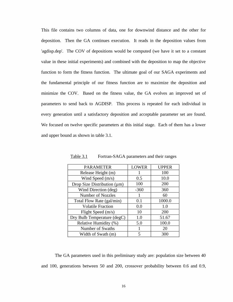
We focused on twelve specific parameters at this initial stage. Each of them has a lower
and upper bound as shown in table 3.1.
Table 3.1 Fortran-SAGA parameters and their ranges
PARAMETER LOWER UPPER Release Height (m) 1 100 Wind Speed (m/s) 0.5 10.0
Drop Size Distribution (µm) 100 200 Wind Direction (deg) -360 360 Number of Nozzles 1 60
Total Flow Rate (gal/min) 0.1 1000.0 Volatile Fraction 0.0 1.0
Flight Speed (m/s) 10 200 Dry Bulb Temperature (degC) 1.0 51.67
Relative Humidity (%) 5.0 100.0 Number of Swaths 1 20
Width of Swath (m) 5 300
The GA parameters used in this preliminary study are: population size between 40
and 100, generations between 50 and 200, crossover probability between 0.6 and 0.9,

17
jump mutation probability between 0.005 and 0.05, and creep mutation probability
between 0.002 and 0.05.
3.4 Results and Discussion of Fortran-Based SAGA
At this stage, we focused on the determination of (hopefully) optimal spray
parameter settings. Some preliminary results are shown in Table 3.2. The GA
parameters used in these experiments are: population size 70; crossover probability 0.8;
mutation probability 0.01, etc. It should be noted that we are dealing with two sets of
parameters: one set for the Fortran GA driver which includes population size,
generations, crossover and mutation probability, and one set for the spray simulation
model which includes release height, drop size, and other spray parameters. From the
evolution of the fitness values, we can see that the Fortran-SAGA has done a good job of
improving the parameter values in order to obtain better depositions. For example,
comparing the depositions at the edge of the spray block, we can see that the deposition
has improved from 98.34 mg/m2 in the first generation to 146.53 mg/m2 after 70
generations.
Table 3.2 An example of preliminary results of Fortran-SAGA
GENERATION DEPOSITION (mg/m2) 1 98.34 5 99.46
10 102.56 20 108.25 30 116.84 40 119.25 50 124.29 60 137.58 70 146.53

18
There were a few simplifications that we embedded during this testing stage such
as setting the COV to a constant value of 0.3, and restricting the droplet size range. The
primary reason for these simplifications was that it allowed us to begin the spray
parameter optimization process and test the feasibility of the project fairly quickly after
setting up the genetic algorithm and its connection with the spray model. The
computation of the COV was not incorporated in the original AGDISP DOS 7.0 and thus
COV was not directly available to be mapped into the fitness function. We felt it might
require implementing another routine to determine the COV. This problem was solved
later by incorporating the computation of COV within a new AGDISP DLL file created
from AGDISP DOS 7.0 (details explained in Chapter 4). The other simplification at this
stage dealt with droplet size distribution. Here we set the range for droplet size to be
between 100µm and 200µm. This range was subdivided into ten droplet size categories
with an increment of 10µm. Each droplet size category was assigned a mass fraction of
0.1. In spray practice the droplet size distribution may be dependent on certain factors
such as nozzle specifications and spray speed. This simplification was also temporary set
for quick start of the spray parameters optimization process. It is not before long that
these simplifications are removed in our later development to obtain more accurate and
reliable results.
We also ran numerous experiments to determine which GA parameters seemed to
produce the best results. The selection of GA parameters such as population size, number
of generations, crossover type and probability, and mutation probability is a key facet of
the speed and success of the evolutionary process. These parameters are typically
domain dependent. One big problem with this initial SAGA was that it was to a certain

19
extent limited by the runtime of AGDISP DOS 7.0. This added the difficulty to change
the population size and generations freely. The runtime of the AGDISP module typically
varies from 5 to 45 seconds for each run depending on the aerial spray parameters and the
working platform. The runtime of the main GA program is negligible compared to the
AGDISP runtime. Thus for example if we set the population size to 50 and number of
generations to 100, then assume an average AGDISP runtime length of 15 seconds, it will
take about 20 hours to complete the SAGA run. During these initial experiments, we
usually let SAGA run overnight and collect data the next morning. Therefore, the
number of generations was accordingly set to around 50 and the population size was set
to between 50 and 100. Table 3.3 shows some comparisons of the results obtained with
different GA population sizes. Similar experiments were run to help determine
appropriate values for other GA parameters.
Table 3.3 Fortran-SAGA results at different population size
GENERATION DEPOSITION (mg/m2)
Population size = 50 Population size = 40 Population size = 20 1 98.34 98.34 98.34
20 108.25 107.36 105.42 50 124.29 122.68 116.35
Another key issue in the initial development of SAGA is the mapping of the
deposition and the COV onto the fitness function. It is highly desired to get the exact
amount of spray material evenly distributed over the spray block. The goal is thus to
maximize the deposition and minimize the COV. We followed the rule of thumb
suggested in [Park82] and set the COV to 0.3 temporarily. We tested and compared
different mapping functions having linear and exponential characteristics, and decided to

20
use the exponential function formulated below and the graph shown in Figure 3.3 for our
initial Fortran-SAGA experiments.
It should be noted that COV is dependent on swath width in most cases, but in the
above formulation, we temporarily fixed the COV and set the goal to maximize
deposition only. Later on we removed this simplification by incorporating the
computation of COV into an AGDISP DLL created from the AGDISP DOS 7.0 and
modified our fitness formulation accordingly (details discussed in chapter 4).
Figure 3.3 Fortran-SAGA fitness function graph
In addition, some other work we did at the initial stage was to test the parameter
sensitivity of AGDISP. The approach we took was to set one of the twelve SAGA
parameters constant and test the impact of this change on the deposition evolution.
Release height, wind direction, and wind speed are the three main parameters we focused
( )( )COVbDepositionaFitness ×−×−−= 04.01exp0.3
Fitness = 3.0-exp(1-0.04K) K=a*Dep.-b*COV (a=0.5 b=1.6) COV=0.3
0
0.5
1
1.5
2
2.5
3
3.5
0 50 100 150 200 250
Deposition (mg/m2)
Fit
nes
s

21
on. The results are presented in Table 3.4. It is indicated that setting the release height
has a large impact on the deposition evolution. Likewise, keeping the wind parameters
constant also has a considerable impact on SAGA results. The trend is consistent with
the results obtained by Teske and Barry [Teske93b], namely that the input parameters for
aerial spray can be ranked in order of importance where release height is more important
than any other parameter. The approach they took to measure the relative importance
was to change an input variable linearly and measure the corresponding relative
sensitivity of the results. Two parameter values, Figure of Merit and Mean Horizontal
Position were used to measure the effectiveness of swath width deposition and the level
of off-target drift, respectively. Our results need further technical verifications compared
to their approach. But the similar trend indicated by our results provided support for the
important roles of these key parameters and their relative importance claimed by these
experts.
Table 3.4 Testing of the Fortran-SAGA parameter importance
GENERATION DEPOSITION
(mg/m2) DEPOSITION
(mg/m2) DEPOSITION
(mg/m2) DEPOSITION
(mg/m2) Release
Height = 75m Wind Direction = 150 degree
Wind Speed = 5.0m/s
1 98.34 97.38 96.52 96.82 10 102.56 100.25 100.34 101.25 20 108.25 104.39 103.95 103.49 40 119.25 112.65 115.87 114.58 60 137.58 120.87 125.75 124.68
Based upon the results and experience from these initial SAGA experiments, we
successfully showed the feasibility of the SAGA project and the preliminary results
helped us to make necessary modifications to improve the program. The main necessary

22
improvements we found about the Fortran-SAGA include the user-interface, the
computation of COV, and the running time. The user interface was not friendly enough
mainly due to the Fortran programming language limitations. The user has to specify all
GA parameters in a text file before the run and the SAGA results are stored in a text file
after the run. It would be much more beneficial if the user was able to specify the GA
parameters on a main interface and view the results directly on the interface too. The
output format of AGDISP DOS 7.0 was also not very convenient for us to trace the COV
and apply it in the SAGA fitness formulation. It would also be advantageous to reduce
the running time of the spray simulation model. Some significant changes were expected
to solve these problems.
We decided to change our GA driver with a new GA implemented with Microsoft
Visual Basic 5.0 to take advantage of the language’s nice interface development features.
The new interfaces of SAGA would highly facilitate the use of SAGA. AGDISP 7.0 was
also replaced with a new AGDISP DLL that returns deposition, COV and the resulting
VMD. The new SAGA was expected to speed up significantly based on the improved
DLL and VB-GA. We also expected to incorporate AGDISP parameter dependencies and
practical application considerations (spray knowledge) into a revised fitness measure.
Detailed explanation of the implementation and features of the new SAGA interfaces will
be introduced in Chapter 4.

23
CHAPTER 4
DEVELOPMENT OF VB-SAGA 1.0
After the initial testing stage with Fortran-SAGA, some significant changes were
made to improve the SAGA user-friendliness and overall performance. We implemented
a new SAGA GA with Microsoft VB 5.0. This new VB-GA features highly user-friendly
interfaces. A new AGDISP DLL created from the AGDISP model was used as the spray
simulation engine. The new SAGA program was named VB-SAGA 1.0. As discussed in
Chapter 3, the inter-connection between the Fortran GA and AGDISP DOS Version 7.0
was established on the reading and writing of intermediate files. In VB-SAGA 1.0 these
files were replaced by inter-program calls that speed up SAGA significantly. Section 4.1
discusses details of the implementation of VB-SAGA 1.0 and its experimental
performance.
As requested by the Forest Service, an exhaustive search scheme was set up to
validate the GA and test/compare the performance of our VB-SAGA. Section 4.2
introduces this exhaustive search scheme and the comparison results.
4.1 VB-SAGA 1.0
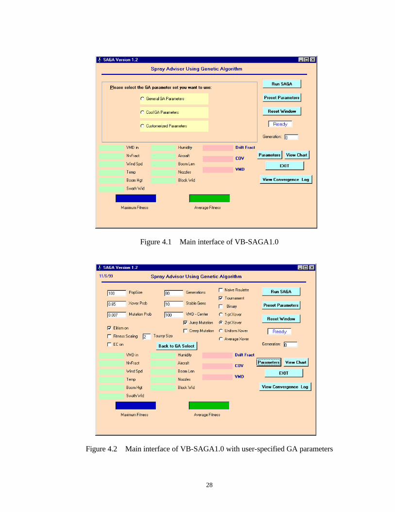
Figures 4.1 to 4.4 show the interfaces of the new VB-SAGA. These interface
windows are designed to provide user convenience and high flexibility to specify GA
parameters, preset necessary spray parameters, chart ongoing SAGA evolution, view the
dynamic evolution of the spray parameters, and view final SAGA results information.

24
The top half of the main interface is primarily for GA control parameters and the bottom
half is mainly for spray parameters and results.
As shown in Figure 4.1, depending on the user’s knowledge of the GA and the
application purpose, the user can select either [General GA Parameters] which is a set of
recommended GA parameters for gypsy moth spray, [Cool GA Parameters] which is a set
of recommended GA parameters for regular spray, or the advanced [Customized GA
Parameters]. If the user selects the [Customized GA Parameters], groups of GA
parameters will appear (shown in Figure 4.2) and the user can modify the default values
as they like.
The new VB Genetic Algorithm driver in this study originated from the Simple
Genetic Algorithm (SGA) described by Goldberg [Gold89]. The GA initializes the first
population with individuals generated at random. An individual corresponds to a set of
AGDISP parameters. We made use of one of the convenient features of VB, the "Type"
statement, to define a new data structure that consists of the eleven spray parameters
(defined as a Single array), three return values from the DLL, and the fitness. This new
data type is named "individual". This “individual” corresponds to the chromosome string
representation in the traditional GA. We use a real number representation for the
parameters and the individuals.
For the GA parameters, as shown in Figure 4.2, we have various GA options that
users can select to group a set of GA parameters for SAGA. The user can enter
population size, generations, crossover probability, and mutation probability into the text
areas. Each of these parameters is provided a default value, e.g., 100 for PopSize, 80 for
Generations, 0.65 for Crossover Probability, and 0.007 for Mutation Probability. For the

25
GA operators, we provide several options for each. For the selection scheme, users can
choose among [Naive Roulette Wheel] selection, [Tournament] selection and [Binary]
selection. For the crossover operation, users have the options of [1-point], [2-point],
[uniform], and [average] crossover. We have [Jump Mutation] and [Creep Mutation] for
mutation options. The former is to randomly select a new value for a parameter within its
valid range. The latter is to change the old parameter by a small increment (error
checking is added to make sure the new value is valid). Besides these basic GA
parameters, we also add some new features such as [Elitism], which will enable the GA
to inherit the best individual from the previous generation when turned on. Another
useful option is [Fitness Scaling] which is an advanced GA feature that is used to
overcome the "local maximum" problem. With [Elitism] and [Fitness Scaling] turned on,
the SAGA normally converges in less than 30 generations. The GA population becomes
basically homogenous after that and there is no necessity to run the program much
longer. We thus provide a [Stable Generations] option for the user to specify how many
stable generations (no changes in maximum fitness) are allowed before stopping SAGA.
The current default value is 12. The user can also specify the tournament size used in the
tournament selection scheme. The recommended value is 2 for selection in pairs.
In practical spray applications, it's quite common that some spray parameters can
and should be fixed according to the spray requirements. We thus provide the option to
preset certain spray parameters by selecting [Preset Parameters]. A new interface
window will appear with the spray parameters listed (shown in Figure 4.3). The user can
select the ones to preset and fill in appropriate values. The rest of the parameters are left
open to evolution by SAGA.

26
The bottom half of the main interface is designed to display intermediate results
with two options provided. The first option is that the user can view the dynamic values
of the eleven spray parameters and the three spray results (shown in Figures 4.1 and 4.2).
These values are associated with the best individual so far as the program evolves from
generation to generation. This option is set as the default output mode. The user can also
click on the [View Chart] button to switch the bottom half to a fitness growth chart with
the maximum and average fitness values displayed dynamically (shown in Figure 4.4).
The user can click on the [View Parameters] to return to the parameters option.
After the user finishes setting the GA and spray parameters, clicking on the [Run
SAGA] button starts the run, or clicking [Reset Window] resets the parameters to their
default values. Besides the spray parameters and results being displayed dynamically in
the main interface, the user can also click on [View Convergence Log] after the program
stops to look at a detailed report.
The spray parameters to be optimized by VB-SAGA1.0 are not the same as those
used in Fortran-SAGA as shown in Table 3.1. As suggested by Forest Service experts,
we introduced several more representative spray parameters such as VMD Input, Aircraft
ID Number, and Block Size. We removed some old parameters such as Number of
Swaths, Drop Size Distribution, and Total Flow Rate. Table 4.1 shows the eleven spray
parameters that are to be optimized by VB-SAGA 1.0. These eleven spray parameters
are also the input parameters for the new AGDISP DLL. Other less important or more
static parameters are kept constant during our experiments. However, they can become
part of the variable parameter set (i.e., we can easily include additional parameters to the
27
parameter set we are searching for) by specifying them at the beginning of each SAGA
run if the user requests so.
Table 4.1 VB-SAGA1.0 spray parameters and their ranges
PARAMETER LOWER UPPER VMD Input (µm) 100 400 Nonvolatile Fraction 0.001 1.0 Wind Speed (m/s) 0.23 4.47 Temperature (degree C) 1 30 Boom Height (m) 3 30 Swath Width (fraction of wingspan) 0.3 3.0 Humidity (%) 0.0 1.0 Aircraft ID Number 1 124 Boom Length (fraction of wingspan) 0.3 1.0 Number of Nozzles 1 60 Block Size (m) 50 1000
The VB-SAGA1.0 has very similar architecture as that of Fortran-SAGA shown
in Figure 3.2. However, there are two major differences. One is that instead of
Deposition and COV, the new AGDISP DLL returns three outputs, Drift Fraction, COV,
and VMD Output. We adopt a new fitness function (shown below) suggested by the
USDA Forest Service experts that incorporates these three outputs with different weights.
VMDCenter is the desired VMD value specified by the user before the run. The other
difference is that the connection between the VBGA and the AGDISP simulation model
is now based on the inter-program calls instead of the I/O intermediate files for the
Fortran-SAGA. This improvement greatly speeds up the SAGA to a large extent.
( )[ ] ( )[ ]
−×−×+−×+−××=
2
10.8exp251250.150100VMDCenter
VMDCOVDriftFracFitness
28
Figure 4.1 Main interface of VB-SAGA1.0
Figure 4.2 Main interface of VB-SAGA1.0 with user-specified GA parameters

29
Figure 4.3 Secondary interface of VB-SAGA1.0 to preset spray parameters
Figure 4.4 VB-SAGA1.0 main interface with chart view option turned on

30
4.2 Exhaustive Search Test and Comparison with VB-SAGA 1.0
4.2.1 Exhaustive Search Test
The exhaustive search test was requested by the Forest Service to validate the GA
and SAGA results. The goal of the test was to compare SAGA results with exhaustive
search results to make sure that SAGA was able to find optimal or near-optimal solutions.
The exhaustive test program interface is shown in Figure 4.5. Because the tremendously
huge search space for eleven parameters, it was desired to finish the exhaustive test with
reasonable time and economical efforts. We thus needed to reduce the huge search space
to run the exhaustive search within several days as long as the results meet the Forest
Service requirements. The approach we took to reduce the huge search space was to fix
eight spray parameters as shown in Table 4.2 and test the remaining combinations of the
other three parameters as shown in Table 4.3. Another effort to reduce the search space
was to use narrower ranges (reduce upper bound and increase lower bound) of these three
parameters. Our earlier test runs gave us some idea of good ranges of these three
parameters, we therefore used these smaller ranges (also shown in Table 4.3) instead of
the full range as shown in Table 4.1. These spray parameters were imported into
AGDISP DLL to produce batch results and we used the same fitness function in SAGA
to obtain their fitness value. The total combination of all parameter sets is about
15*12*100=18,000. If we estimate an average running time to be about 20 seconds for
each run, the total running time for the exhaustive test will be approximately 4 days. The
actual exhaustive search experiment took about three and one half days and the top ten
solutions are listed in Table 4.4.

31
Figure 4.5 Exhaustive search test main interface
Table 4.2 Fixed spray parameters in exhaustive search test
DSD-VMD 100.0 micron Temp 10.0 degC
Humidity 75.0 AircraftNum 7 BoomWidth 0.75
NumNoz 42 BlockWidth 400.0 m SwathWidth 1.2 m
Table 4.3 Changing spray parameters in exhaustive search test
Lower Bound Upper Bound Increment Step
NvFrac 0.75 0.9 0.01 Wind Speed 0.23m/s 0.35m/s 0.01 BoomHeight 6.0m 7.0m 0.01

32
Table 4.4 Fitness results from exhaustive experiment (8 fixed parameters)
NO. BEST FITNESS
1 9428.176 2 9427.911 3 9427.605 4 9427.257 5 9426.553 6 9426.434 7 9425.577 8 9425.041 9 9423.479 10 9422.863
It should be noted that the exhaustive experiment results are dependent on the
increment step adopted. The exhaustive test scheme being used here is in fact a pseudo
exhaustive search, because we are actually selecting very closely spaced points in the
search space, though the difference between the points is very small to match as close as
possible to a real exhaustive search. However, the problem does exist that using this
pseudo exhaustive search could possibly leave out some good points and reduce the
certainty of finding the best individual. We therefore need to minimize the steps to the
smallest possible in order to approach closely enough to a continuous search in order to
obtain best results. However, the smaller the steps are, the longer time it will take to
finish the exhaustive search. We want to complete the experiment within a reasonable
time length as long as the results satisfy the precision requirements. For our testing
purpose and precision requirements, we think the step 0.01 is acceptable for all three
changing parameters and the results are satisfactory to validate the GA and SAGA.

33
4.2.2 VB-SAGA1.0 Test
We then ran VB-SAGA1.0 with the same eight spray parameters fixed with the
same values, and let VB-SAGA1.0 evolve Non Volatile Fraction, Wind Speed, and Boom
Height to obtain their best values as well as the best spray results. The results are
displayed in Table 4.5. It only took 1.5 hours to finish and the best result from SAGA
was found among the top 0.1% of the exhaustive results. Table 4.6 shows a side-by-side
comparison of best exhaustive with best SAGA results. This is a good validation that
SAGA is capable of finding near-optimal solutions for our spray application in relatively
short time.
Table 4.5 Fitness results from VB-SAGA 1.0 experiment (8 fixed parameters)
MUT.
XOVER
0.001 0.003 0.007 0.01 0.02 0.03 ROW AVG.
0.60 9384.353 9329.302 9354.186 9345.647 9407.326 9416.380 9372.866 0.65 9322.343 9392.962 9399.037 9416.356 9406.362 9324.382 9376.907 0.70 9402.429 9400.000 9406.360 9387.536 9395.794 9351.680 9390.633 0.75 9403.283 9358.872 9401.998 9364.615 9404.165 9398.096 9388.505 0.80 9423.766 9411.717 9393.582 9413.530 9417.993 9397.563 9409.692 0.85 9321.064 9335.679 9427.255 9414.876 9396.127 9358.782 9375.631
COLUMN AVG.
9376.206 9371.422 9397.07 9390.427 9404.628 9374.481
Table 4.6 The maximum fitness for exhaustive and VB-SAGA 1.0 tests
EXHAUSTIVE TEST GA TEST Maximum Fitness 9428.176 9427.255
Non-Volatile Fraction 0.780 0.789 Wind Speed (m/s) 0.280 0.282 Boom Height (m) 6.100 5.777
Drift Fraction 0.0309 0.0297 COV 0.165 0.167
VMD (micron) 101.625 104.223

34
4.3 VB-SAGA1.0 Experiments and Results
After the exhaustive validation test, we began to use VB-SAGA 1.0 under
different circumstances, mainly with and without spray parameter restrictions. We ran
many experiments based on particular specifications by the Forest Service for their
practical applications.
4.3.1 VB-SAGA1.0 Best Result with No Spray Parameter Restrictions
With no spray parameters fixed, SAGA is expected to generate better results
compared to those with certain spray parameter restrictions. The best fitness and the
corresponding spray parameters are listed in Table 4.7.
Table 4.7 The maximum fitness from VB-SAGA 1.0 without restrictions on spray parameters (GA crossover rate=0.65 and mutation rate=0.007)
ITEM BEST RESULTS Maximum Fitness 9924.08
DSD-VMD (micron) 100 Non-Volatile Fraction 0.788
Wind Speed (m) 0.264 Temperature (degC) 4.941
Humidity (%) 62.715 Aircraft 110
Boom Length (fraction of wingspan) 0.529 Nozzles 9
Boom Height (m) 7.086 Block Size (m) 964.9
Swath Width (fraction of wingspan) 0.543 Drift Fraction 0.00301
COV 0.0242 VMD (micron) 99.58

35
4.3.2 VB-SAGA1.0 Results with Certain Spray Parameter Restrictions
We ran many experiments based on the practical spray parameter specifications
provided by Forest Service managers. In total there are six groups of experiments that
belong to two categories. The first category includes two groups of experiments of which
four and seven spray parameters are fixed respectively. The second category includes the
other four groups of experiments that focus on investigating the roles of aircraft and
swath width. For each group, we ran 10 experiments with the combination of crossover
rate 0.65, 0.7, 0.75, 0.8, 0.85 and mutation rate 0.007 and 0.012. The population size is
100 and the generation is 70 for all experiments.
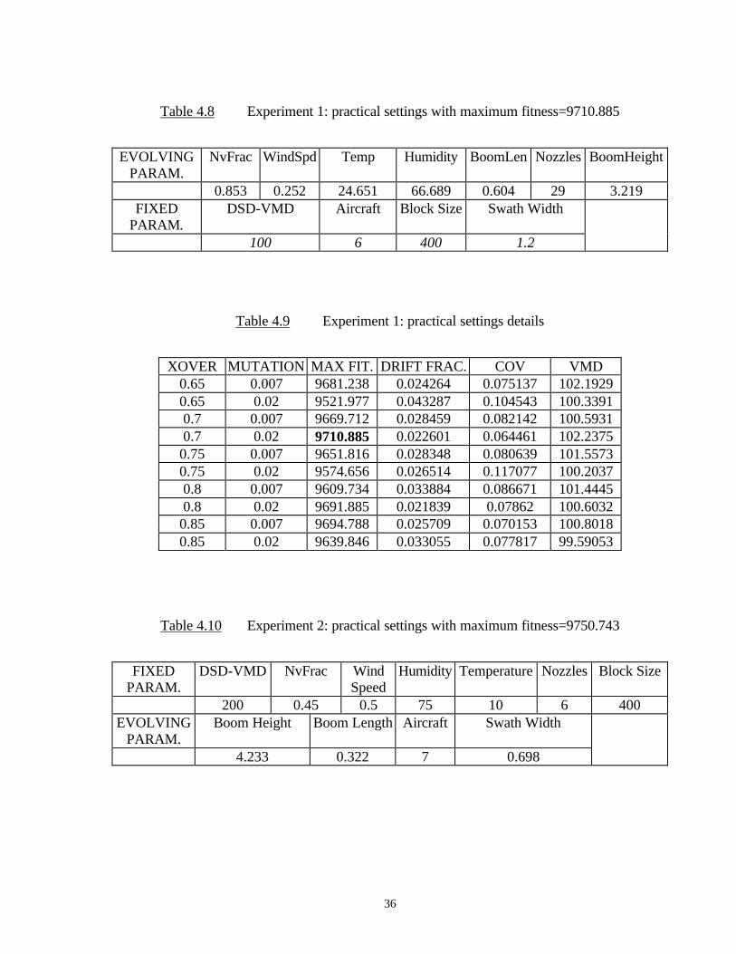
The maximum fitness obtained based on the first group of specifications was
9710.885 and the spray parameters corresponding to this maximum fitness are listed in
Table 4.8. Detailed results are listed in Table 4.9. DSD-VMD, Aircraft, Block Size and
Swath Width were fixed in this case. The second group of experiments has the highest
fitness of 9750.743 and its corresponding spray parameters are listed in Table 4.10.
Detailed results are listed in Table 4.11. DSD-VMD, Aircraft, Block Size and Swath
Width are fixed in this case.
Besides the above two groups of experiments, we also ran four groups of
experiments with different configurations of fixed aircraft and swath width. Tables 4.12
to 4.15 show the results from these four groups of experiments. It is often a matter of fact
that the aircraft has to be fixed due to availability restriction during spray practice. It is
therefore of highly practical importance to determine what optimal or near optimal values
for other parameters should be used when the aircraft and swath width are fixed. These
four groups of experiments were expected to give the forest managers such possible help.
36
Table 4.8 Experiment 1: practical settings with maximum fitness=9710.885
EVOLVING PARAM.
NvFrac WindSpd Temp Humidity BoomLen Nozzles BoomHeight
0.853 0.252 24.651 66.689 0.604 29 3.219 FIXED
PARAM. DSD-VMD Aircraft Block Size Swath Width
100 6 400 1.2
Table 4.9 Experiment 1: practical settings details
XOVER MUTATION MAX FIT. DRIFT FRAC. COV VMD 0.65 0.007 9681.238 0.024264 0.075137 102.1929 0.65 0.02 9521.977 0.043287 0.104543 100.3391 0.7 0.007 9669.712 0.028459 0.082142 100.5931 0.7 0.02 9710.885 0.022601 0.064461 102.2375
0.75 0.007 9651.816 0.028348 0.080639 101.5573 0.75 0.02 9574.656 0.026514 0.117077 100.2037 0.8 0.007 9609.734 0.033884 0.086671 101.4445 0.8 0.02 9691.885 0.021839 0.07862 100.6032
0.85 0.007 9694.788 0.025709 0.070153 100.8018 0.85 0.02 9639.846 0.033055 0.077817 99.59053
Table 4.10 Experiment 2: practical settings with maximum fitness=9750.743
FIXED PARAM.
DSD-VMD NvFrac Wind Speed
Humidity Temperature Nozzles Block Size
200 0.45 0.5 75 10 6 400 EVOLVING
PARAM. Boom Height Boom Length Aircraft Swath Width
4.233 0.322 7 0.698

37
Table 4.11 Experiment 2: practical settings details
CROSSOVER MUTATION MAX FIT DRIFT FRAC COV VMD 0.65 0.007 9643.027 0.010314 0.065517 217.0752 0.65 0.02 9021.266 0.040434 0.096909 234.6726 0.7 0.007 9623.292 0.014304 0.063063 217.4393 0.7 0.02 9250.907 0.028835 0.098085 227.8699
0.75 0.007 9750.743 0.074591 0.030589 216.6913 0.75 0.02 9642.524 0.011115 0.06124 217.5165 0.8 0.007 9642.524 0.011115 0.06124 217.5165 0.8 0.02 9263.371 0.029171 0.099688 227.102
0.85 0.007 9263.371 0.029171 0.099688 227.102 0.85 0.007 9551.506 0.011498 0.071744 221.0305
Table 4.12 Experiment 3: practical settings details (Aircraft: 100, swath width: 2.5)
XOVER MUTATION MAX FIT COV VMD DRIFT FRAC 0.65 0.02 8478.91 0.4693 206.174 0.06913 0.65 0.007 8489.09 0.4747 200.007 0.0648 0.7 0.02 8492.34 0.468 200.104 0.0674 0.7 0.007 8486.53 0.442 199.89 0.0812
0.75 0.02 8476.31 0.4767 199.95 0.0663 0.75 0.007 8489.97 0.468 199.79 0.0673 0.8 0.02 8488.16 0.4343 199.23 0.0833 0.8 0.007 8492.53 0.4625 199.769 0.06967
0.85 0.02 8494.48 0.4673 199.91 0.06722 0.85 0.007 8477.4 0.4476 199.708 0.07998

38
Table 4.13 Experiment 4: practical settings details
(Aircraft: 106, swath width: 2.25)
XOVER MUTATION MAX FIT COV VMD DRIFT FRAC 0.65 0.02 8717.63 0.384 199.37 0.063 0.65 0.007 8728.38 0.3798 199.434 0.063 0.7 0.02 8716.13 0.385 199.292 0.0625 0.7 0.007 8730.29 0.378 199.44 0.0634
0.75 0.02 8730.85 0.378 199.42 0.0636 0.75 0.007 8719.01 0.381 199.244 0.064 0.8 0.02 8738.82 0.377 200.112 0.06346 0.8 0.007 8729.69 0.375 199.565 0.654
0.85 0.02 8720.44 0.383 199.39 0.063 0.85 0.007 8730.54 0.375 199.52 0.0652
Table 4.14 Experiment 5: practical settings details (Aircraft: 5, swath width: 2.3)
XOVER MUTATION MAX FIT COV VMD DRIFT FRAC 0.65 0.02 8345.86 0.362 200.33 0.198 0.65 0.007 8345.78 0.36 200.77 0.149 0.7 0.02 8346.01 0.362 201.18 0.147 0.7 0.007 8351.57 0.362 200.2 0.15 0.75 0.02 8351.86 0.363 200.404 0.147 0.75 0.007 8353.54 0.36 200.17 0.148 0.8 0.02 8349.72 0.36 200.3 0.149 0.8 0.007 8353.4 0.361 200.3 0.148 0.85 0.02 8357.87 0.3607 200.27 0.1474 0.85 0.007 8354.77 0.3608 200.078 0.14844

39
Table 4.15 Experiment 6: Practical Settings Details
(Aircraft: 10, swath width: 2.2)
XOVER MUTATION MAX FIT COV VMD DRIFT FRAC
0.65 0.02 8441.29 0.3694 200.12 0.127 0.65 0.007 8353.47 0.357 199.08 0.148 0.7 0.02 8405.04 0.378 201.7 0.13 0.7 0.007 8432.74 0.368 199.777 0.1291
0.75 0.02 8438.65 0.3689 199.655 0.1269 0.75 0.007 8434.23 0.37 200.5 0.128 0.8 0.02 8444.23 0.37 199.93 0.126 0.8 0.007 8440.37 0.365 199.989 0.129
0.85 0.02 8436.35 0.371 200.82 0.125 0.85 0.007 8439.76 0.362 200.111 0.13
These results were evaluated by spray experts and regarded as excellent
predictions with high practical importance. More experiments are to be run to test other
scenarios and the results are expected to assist practical spray applications, including
selecting optimal spray conditions, estimating spray results, reducing spray cost, and
minimizing spray drift.

40
CHAPTER 5
DEVELOPMENT OF VB-SAGA 2.0
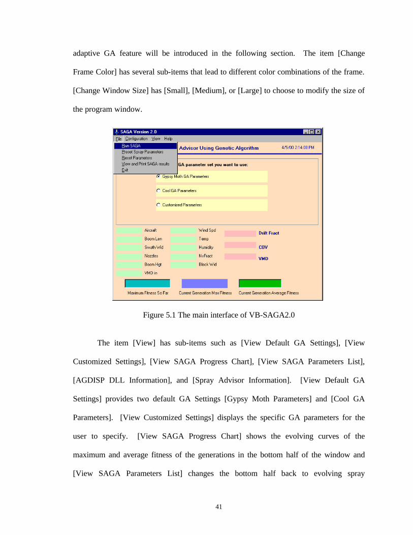
VB-SAGA2.0 inherits most important features of VB-SAGA1.0 and adds some
significant new features. The two most important new features are the menu and the self-
adaptive GA. Figure 5.1 shows a typical VB-SAGA 2.0 interface with these two new
features. In addition, VB-SAGA2.0 uses a slightly modified fitness function listed
below.
5.1 VB-SAGA2.0 Menu Items
VB-SAGA2.0 replaced the buttons of VB-SAGA1.0 with a menu bar as shown in
Figure 5.1. All the functionality of the buttons on the VB-SAGA1.0 main interface is
now replaced by this handy menu bar. The menu bar is added onto the top-left corner of
the VB-SAGA 2.0 main interface. The four main menus on the menu bar are
[Command], [Configuration], [View], [Help]. Each main menu has certain sub-items.
For example, under the [Command] item, there are [Run SAGA], [Preset Spray
Parameters], [Reset Parameters], [View and Print SAGA Results], and [Exit].
Under the [Configuration] item, there are [Enable Adaptive GA], [Disable
Adaptive GA], [Change Frame Color], and [Change Window Size]. The adaptive GA
feature can be enabled and disabled by selecting the first or second item. Details of the
[ ] [ ] [ ]{ }
−−=
+−×+−××=
VMDCenter
VMDAbsVMDTerm
VMDTermCOVDriftFracFitness
0.10.1
*25)1(25)0.1(50100
41
adaptive GA feature will be introduced in the following section. The item [Change
Frame Color] has several sub-items that lead to different color combinations of the frame.
[Change Window Size] has [Small], [Medium], or [Large] to choose to modify the size of
the program window.
Figure 5.1 The main interface of VB-SAGA2.0
The item [View] has sub-items such as [View Default GA Settings], [View
Customized Settings], [View SAGA Progress Chart], [View SAGA Parameters List],
[AGDISP DLL Information], and [Spray Advisor Information]. [View Default GA
Settings] provides two default GA Settings [Gypsy Moth Parameters] and [Cool GA
Parameters]. [View Customized Settings] displays the specific GA parameters for the
user to specify. [View SAGA Progress Chart] shows the evolving curves of the
maximum and average fitness of the generations in the bottom half of the window and
[View SAGA Parameters List] changes the bottom half back to evolving spray
42
parameters. [AGDISP DLL Information] gives some introduction of the AGDISP model
and its DLL version.
The item [Help] has sub-items such as [View Help File], [View Recent SAGA
Paper], [View General GA Tutorial], and [Contact Information]. [View Help File]
enables the user to view an introduction document about SAGA. [View Recent SAGA
Paper] presents the user with the latest published SAGA paper so that the user can have
comprehensive knowledge of the development and achievements of SAGA. [View
General GA Tutorial] provides a quick tutorial about basic concepts and working
principles of the GA. [Contact Information] provides the authors information for
comments or inquiries.
5.2 The Self-adaptive GA
5.2.1 Why use the self-adaptive GA
SAGA1.0 has shown steady and satisfactory performance. However, we expect it
to have better performance for all levels of users. For example, the program requires
certain computer and GA knowledge by the user, especially knowledge about setting
appropriate GA parameters before the run. The rule of thumb for the best values of the
GA parameters is 0.65 - 0.85 for crossover rate, 0.005 – 0.01 for mutation rate. Our
previous experiments showed that for SAGA, crossover rate between 0.75 and 0.85 and
mutation rate between 0.005 and 0.012 usually produced good results. But the specific
values may differ with different problems. For an inexperienced user, it may take many
tests before locating the appropriate range and exact values of these GA parameters. This
is not always welcome, especially in the situation when the operation time is a major

43
concern. It is also not easy for a novice user to understand the GA concepts such as
crossover and mutation quickly. One main goal of our project is that the user with little
GA knowledge can start to use SAGA quickly and correctly. We thus continued our
efforts to develop an improved SAGA with a self-adaptive GA feature such that some
users with little GA knowledge or even little computer knowledge are able to use SAGA
easily. We name the new program VB-SAGA2.0. With this self-adaptive GA feature on,
the new VB-SAGA2.0 can actually start at any random valid GA operator values (for
crossover and mutation only at this stage), the program will evolve to the best GA values
as well as the best spray parameters.
5.2.2 Fuzzy logic control
Fuzzy Logic is basically a multi-valued logic that is used to handle the concept of
partial truth instead of "completely true" and "completely false" notions such as yes/no,
true/false, and black/white [Kosk91]. By using fuzzy logic, notions like small, big,
warm, or pretty cold can be formulated mathematically and processed by computers.
Fuzzy logic was first introduced by Dr. Lotfi Zadeh at UCBerkeley in the 1960's as a
means to model the uncertainty of natural language [Neuy99]. It has emerged as a
powerful tool for the control of subway systems and complex industrial processes, as well
as for household and entertainment electronics, diagnosis systems and other expert
systems.
The membership function is one of the important concepts in fuzzy logic. It is
used to convert an input to be anywhere in the range of [0, 1] [Neuy99]. Triangular or
Gaussian functions are commonly used representations of membership functions. A set

44
of IF-THEN rules is used in fuzzy logic to stipulate what actions should be taken under
certain conditions. Fuzzification is the process used to convert crisp inputs to values in
the range of [0, 1] (degree of the membership) based on the membership functions. If the
fuzzified values match the conditions of one or more rules, the actions of these rules will
be taken to produce outputs. If more than one rule is fired, the outputs need to be
aggregated together to generate an output region. Defuzzification is the last process in
fuzzy control to deduce the crisp output from the output region. Centroid, maximizer,
and weighted average are the three commonly used approaches to locate crisp output.
5.2.3 Development of self-adaptive GA in VB-SAGA2.0
The idea for the self-adaptive GA came from the work by Lee and Takagi
[Lee93]. They use fuzzy logic techniques to dynamically control parameter settings of
their GA. We simplified their approach and designed our adaptive scheme based on
similar principles. For our self-adaptive SAGA, there are three inputs and two outputs.
The three inputs are:
A1: (average fitness)/(best fitness)
A2: (worst fitness)/(average fitness)
A3: change in fitness since last generation
The two outputs are:
B1: the crossover probability change
B2: the mutation probability change
Each input or output has three membership values: small, medium and big.
Triangular membership functions are used for this fuzzy control (the membership

45
functions are listed in Appendix A). There are altogether 27 control rules for our self-
adaptive GA (listed in Appendix B). Some examples of the rules are as follows:
IF A1 is small, A2 is small, and A3 is small, THEN B1 is small and B2 is small.
IF A1 is small, A2 is medium, and A3 is medium, THEN B1 is big and B2 is
medium.
IF A1 is medium, A2 is small, and A3 is medium, THEN B1 is medium and B2 is
big.
When the self-adaptive feature is turned on, the GA watches the changes of A1,
A2 and A3, and makes modifications to B1 and B2 when one or more rules are fired. We
use triangular membership functions in fuzzification and defuzzification to obtain crisp
outputs. The goal is to force the GA to evolve to the GA parameters that maximize the
fitness based on the underlying rules. The new crossover and mutation parameters are
restricted such that they can at most change half of their previous values every time. The
valid ranges for both crossover and mutation rates are [0, 1].
5.3 Results of VB-SAGA2.0
Table 5.1 gives an example of the best fitness from VB-SAGA2.0 with the self-
adaptive GA feature on. In this example, the VB-SAGA2.0 started at population 100,
generation 70, crossover 0.75, mutation 0.012, and VMD-target 100. No spray parameter
restrictions in this case. The best fitness obtained is 9935.24 and the corresponding best
spray parameters are also shown in the table. The final crossover rate is 0.9203 and
mutation rate is 0.0125 due to self-adaptive change. The best fitness from SAGA1.0 with
same initial conditions is also listed in the table for comparison.

46
We then ran two experiments to test SAGA2.0 performance with the same initial
spray conditions of experiment 1 and 2. That is, for experiment 1, we fixed DSD-VMD,
Aircraft Number, Block Size, and Swath Width, while other spray parameters were left to
be evolved by SAGA. Experiment 2 was repeated for SAGA2.0 with the same initial
conditions as well. The results are shown in Table 5.2. The best fitness results from the
two experiments of SAGA1.0 are also listed for comparison.
We further ran several more tests with SAGA2.0 repeating conditions of
experiment 3 to 6 to compare the performance of SAGA1.0 and SAGA2.0. Table 5.3
gives the details of the results.
Table 5.1 Results from VB-SAGA 1.0 and VB-SAGA 2.0
MAX FIT COV VMD DRIFT FRAC VB-SAGA1.0 9924.08 0.0242 99.58 0.00301 VB-SAGA2.0 9935.24 0.0215 100.73 0.00312
Table 5.2 VB-SAGA 2.0 results for experiment 1 and 2
EXPERIMENT MAX FIT COV VMD DRIFT FRAC. SAGA1.0 BEST FIT. 1 9788.236 0.0632 102.132 0.0223 9710.885 2 9802.384 0.0312 205.434 0.0651 9750.743
Table 5.3 VB-SAGA2.0 results for experiment 3-6
EXPERIMENT
AIRCRAFT SWATH WIDTH
MAX FIT.
COV VMD DRIFT FRAC.
SAGA1.0 BEST FIT.
3 106 2.25 9500.97 0.141 200.56 0.02797 8738.82 4 100 2.5 9327.26 0.265 200.25 0.03841 8494.48 5 10 2.2 9405.37 0.149 200.17 0.1536 8444.23 6 5 2.3 8386.54 0.213 199.85 0.01257 8357.87
47
As we can see from Tables 5.2 and 5.3, the self-adaptive SAGA2.0 has obtained
significantly better results than the regular SAGA1.0 for experiment 3 to 6. However, in
Table 5.3, the results of the self-adaptive SAGA2.0 are only a little better than those of
the regular SAGA1.0 for experiments 1 and 2. One of the reasons for this difference is
the degree of the spray parameter restrictions. Experiments 1 and 2 fixed four and seven
spray parameters respectively, while experiments 3 to 6 fixed two parameters only. As
we know, the crossover and mutation operators apply on individuals to exchange their
characteristics and maintain certain diversity. If many spray parameters are already
fixed, the effect of crossover and mutation will be reduced by a large extent. The self-
adaptive GA in particular relies more on the proper functioning of crossover and
mutation operators to optimize crossover and mutation as well as optimize spray
parameters as the regular VB-SAGA1.0 does.
The self-adaptive GA is the latest addition to our SAGA project. We are still
working on it to run more experiments to verify the results and attempt to improve the
program based on the results and feedback. The adaptive GA has already been proven a
feasible way to improve GA performance [Lee93]. However, the implementation
approach for different problems may differ greatly. Our results of dynamic control of
GA parameters in SAGA have indicated that this new feature can improve SAGA
performance under our circumstances. We are expecting to add new dynamic control
features in future improvements.

48
CHAPTER 6
SUMMARY AND CONCLUSIONS
The development of SAGA consists of three stages as discussed in earlier
chapters, Fortran-SAGA, VB-SAGA1.0, and VB-SAGA2.0. The experimental results
from these different versions of SAGA were evaluated by the spray experts and regarded
as good predictions for practical applications. By using SAGA, the user is able to find
optimal or near-optimal spray parameters in order to achieve minimal drift loss, even
deposition and desired droplet size. SAGA can usually find the optimal or near-optimal
spray parameters in a few hours. If the user presets one or more of the spray parameters,
SAGA will spend even less time to find the optimal/near-optimal values due to the
reduced complexity of the problem. The user is also able to use SAGA as a regular spray
simulation program by specifying some or all spray parameters to obtain spray results,
such as drift fraction, VMD and COV. The newly added user-friendly features such as
the menu bar, and the self-adaptive GA are also highly welcome by the Forest Service
users.
Based on the users’ feedback, we will be able to make further modifications to the
user interface and the program operation. The USDA Forest Service is working on
improving the AGDISP simulation model to speed up SAGA. A revised fitness
formulation is also being proposed by the Forest Service to map the spray results to the

49
fitness as close as possible. In addition, we are making continuous efforts to improve the
GA as well as the overall user friendliness.
One new goal of interest is to apply SAGA to optimize more practical factors in
spray practice such as the time and cost. An example of important factors affecting the
spray time and cost is the flight path of the spraying aircraft. We currently assume the
number of flight lines is determined by dividing the block width by the swath width and
the aircraft follows these flight lines. However, many blocks have irregular shapes. The
problem of flying these blocks is similar to the famous traveling salesperson problem
where a salesperson is expected to visit a group of cities in such an order that the total
traveling distance is minimized. We expect to add this new optimization procedure to
SAGA so that it will be able to find the optimal or near-optimal flight path to reduce
spray time and cost.
It is also one of our future expectations to incorporate a multi-objective GA into
our SAGA project. Our current work focuses on optimizing spray parameters to achieve
maximal spray deposition, minimal evaporation loss, and even spray distribution. We
combine all these objectives into one single fitness function. This approach is often said
to have the drawback of modeling the original problem in an inadequate manner
[Coel94]. Approaches such as min-max optimum [Coel94], combination of the Pareto
method with weights [Cvet99], and ranked solutions based on Pareto-optimal theory
[Dick97] have been taken to tackle such multi-objective problems. We plan to consider
the feasibility of including multi-objective optimization in our future SAGA work.
Our work was (and will be) presented at several AI conferences [Potter99],
[Pott00], [Bi00] as successful GA and AI practical applications. It is also under

50
consideration to be incorporated into the large Spray Advisor package that is used
nationwide by the USDA Forest Service.

51
BIBLIOGRAPHY
[Bi00] Bi, W., W. D. Potter, D. Twardus, H. Thistle, J. Ghent, M. Twery, and M. Teske (2000), “Aerial Spray Optimization”, IC-AI 2000, Las Vegas, NV, July 2000. [Bila84] Bilanin, A. J. and M. E. Teske 1984: “Numerical Studies of the Deposition of Material Released from Fixed and Rotary Wing Aircraft”, NASA CR 3779 [Bila89] Bilanin, A. J., M. E. Teske, J. W. Barry and R. B. Ekblad (1989). “AGDISP: The Aircraft Spray Dispersion Model, Code Development and Experimental Validation”. Transactions of the ASAE 32(1): 327-334. [Burg99] Burgess, C. J., A. J. Chalmers, (1999), “The Optimization of Irregular Computer Architectures Using Genetic Agorithms”, Baltzer Journals, 1999. [Chan83] Chandrasekaran, B., and S. Mittal (1983). “Deep versus Compiled Knowledge Approaches to Diagnostic Problem Solving,” in the International Journal of Man-Machine Studies, Vol. 19, No. 5, pp. 425-436, November. [Coel94] Coello, C. A. C., M. Dudnick, and A. D. Christiansen, “Using Genetic Algorithms for Optimal Design of Trusses”, Proceedings of the Sixth International Conference on Tools with Artificial Intelligence, p88-94, New Orleans, LA, Nov. 1994. [Cvet99] Cvetkovic, D., and I. C. Parmee, “Genetic Algorithm-based Multi-objective Optimization and Conceptual Engineering Design” in the CEC’99, Washington D.C., July 1999. [Davi91] Davis, L., (ed.) (1991). Handbook of Genetic Algorithms, Van Nostrand Reinhold, New York. [DeJo89] De Jong, K. A., W. M. Spears, "Using Genetic Algorithms to Solve NP-Complete Problems", Proceedings of the Third International Conference on Genetic Algorithms, 1989 [Dick97] Dick, R. P., and N. K. Jha, “MOGAC: A Multiobjective Genetic Algorithm for the Co-Synthesis of Hardware-Software Embedded Systems”in Volume 1, IEEE 1997. [Gold89] Goldberg, D.E. (1989). Genetic Algorithms in Search, Optimization, and Machine Learning, Addison-Wesley Publishing Co.

52
[Holl75] Holland, J.H. (1975). Adaptation in Natural and Artificial Systems, Ann Arbor: The University of Michigan Press. [Jog89] Jog, P., J.Y. Suh, and D.V. Gucht (1989). “The Effects of Population Size, Heuristic Crossover and Local Improvement on a Genetic Algorithm for the Traveling Salesman Problem,” in the Proceedings of the 3rd International Conference on Genetic Algorithms, Morgan Kaufmann Publishing, San Mateo, CA. [Kosk91] Kosko, B., (1991) Neural Networks and Fuzzy Systems, a Dynamical Systems Approach to Machine Intelligence, Prentice Hall, Englewood Cliffs, NJ. [Lee93] Lee, M. A., and H. Takagi (1993). “Dynamic Control of Genetic Algorithms using Fuzzy Logic Techniques”, in the Proceeding of 5th Int’l Conference on Genetic Algorithms (ICGA’93), Urbana-Champaign, IL, pp.76-83, July 17-21, 1993. [Levi96] Levine, D. (1996), “Application of a Hybrid Genetic Algorithm to Airline Crew Scheduling”. [McDe81] McDermott, J. (1981). “R1: The Formative Years,” In AI Magazine, Vol. 2, No. 2. [Mich92] Michalewicz, Z. (1992), Genetic Algorithms + Data Structures = Evolution Programs, Spinger-Verlag, New York, NY. [Mirk99] Mirkovic, J., D. Cvetkovic, et. al., "Genetic Algorithms for Intelligent Internet Search: A Survey and a Package for Experimenting with Various Locality Types", IEEE TCCA Newsletter, 1999. [Mitt89] Mittal, S., and F. Frayman (1989). “Towards a generic model of configuration tasks,” in the Proceedings of the Eleventh International Joint Conference on Artificial Intelligence, Vol. 2, pp. 1395-1401. [Neuy99] Neuyen, H. T., E. Walker, "A First Course in Fuzzy Logic", CRCS Publications , 1999 [Pabi96] Parbico, J. P., “ A Genetic Algorithm Approach for the Determination of Cultivar Coefficients in Crop Models”, UGA MS thesis, Athens, GA, 1996. [Park82] Parkin, C.S., and J.C. Wyatt (1982). “The Determination of Flight-Lane Separations for the Aerial Application of Herbicides,” in Crop Protection, 1 (3), pp. 309-321. [Parm99] Parmee, I.C., and C. Dragan, “Use of Preferences for GA-based Multi-objective Optimization”, in GECCO’99, Orlando, FL, 1999

53
[Pott90] Potter, W.D., J.A. Miller, and O.R. Weyrich (1990). “A Comparison of Methods for Diagnostic Decision Making,” in Expert Systems with Applications: An International Journal, vol. 1, pp. 425-436. [Pott91] Potter, W.D., J.A. Miller, B.E. Tonn, R.V. Gandham, and C.N. Lapena (1991). “Improving the Reliability of Heuristic Multiple Fault Diagnosis Via The Environmental Conditioning Operator,” in the International Journal of Applied Intelligence, vol. 2, pp. 5-23. [Pott92] Potter, W.D., R. Pitts, P. Gillis, J. Young, and J. Caramadre (1992) “IDA-NET: An Intelligent Decision Aid for Battlefield Communication Network Configuration,” in the Proceedings of the Eighth IEEE Conference on Artificial Intelligence for Applications (CAIA’92), pp. 247-253. [Pott99] Potter, W.D., W. Bi, D. Twardus, H. Thistle, J. Ghent, M. Twery, and M. Teske (1999), “Intelligent Decision Support for US Forest Aerial Spray”, AAAI annual conference, Orlando, FL. [Pott00] Potter, W.D., W. Bi, D. Twardus, H. Thistle, J. Ghent, M. Twery, and M. Teske (2000) “Intelligent Decision Support for US Forest Aerial Spray Optimization”, IEA-EIA Conference, New Orleans [Teske89] Teske, M.E., Curbishley, T.B. (1989), “Forest Service Aerial Spray Computer Model FSCBG 4.0 User Manual”, C.D.I. Report No. 90-06. [Teske93a] Teske, M.E., Bowers, J.F., Rafferty, J.E., and Barry, J.W., (1993). “FSCBG: An Aerial Spray Dispersion Model for Predicting the Fate of Released Material Behind Aircraft” in Environmental Toxicology and Chemistry, Vol. 12, pp. 453-464. [Teske93b] Teske, M.E. and J.W. Barry (1993). “Parameter Sensitivity in Aerial Application” in Transactions of the ASAE, Vol.36(1), pp. 27-33. [Teske97] Teske, M.E., “A User’s Guide to AgDRIFTTM 1.0: A Tiered Approach for the Assessment of Spray Drift of Pesticides”, eight draft, June 1997. [Teske98a] Teske, M.E. (1998) “AGDISP DOS Version 7.0 User Manual”. [Teske98b] Teske, M. E., H. W. Thistle and B. Eav. (1998a) “New Ways to Predict Aerial Spray Deposition and Drift,” in Journal of Forestry 96(6):25-31.
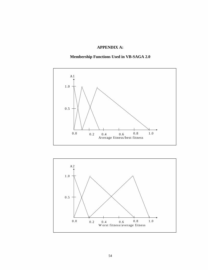
54
APPENDIX A:
Membership Functions Used in VB-SAGA 2.0
0.40.0 0.8
1.0
0.5
1.00.2 0.6Average fitness/best fitness
A1
0.40 .0 0 .8
1 .0
0 .5
1 .00 .2 0 .6W orst f i tness/average f i tness
A 2

55
0.5 2.0
1.0
0.5
1.01.0 1.50.0
Change of crossover rate
B1
1800 300
1.0
0.5
36060 240Change of best fitness
A3
120

56
1.50.5 2.0
1.0
0.5
2.51.0Change of mutation rate
B2

57
APPENDIX B:
Fuzzy Control Rules in VB-SAGA2.0
Rule 1:
IF A1 is small, A2 is small, and A3 is small, THEN B1 is small and B2 is small.
Rule 2:
IF A1 is small, A2 is small, and A3 is medium, THEN B1 is small and B2 is
small.
Rule 3:
IF A1 is small, A2 is small, and A3 is big, THEN B1 is small and B2 is medium.
Rule 4:
IF A1 is small, A2 is medium, and A3 is small, THEN B1 is medium and B2 is
small.
Rule 5:
IF A1 is small, A2 is medium, and A3 is medium, THEN B1 is big and B2 is
medium.
Rule 6:
IF A1 is small, A2 is medium, and A3 is big, THEN B1 is medium and B2 is big.
Rule 7:
IF A1 is small, A2 is big, and A3 is small, THEN B1 is medium and B2 is
medium.
Rule 8:

58
IF A1 is small, A2 is big, and A3 is medium, THEN B1 is small and B2 is
medium.
Rule 9:
IF A1 is small, A2 is big, and A3 is big, THEN B1 is small and B2 is medium.
Rule 10:
IF A1 is medium, A2 is small, and A3 is small, THEN B1 is medium and B2 is
medium.
Rule 11:
IF A1 is medium, A2 is small, and A3 is medium, THEN B1 is medium and B2 is
big.
Rule 12:
IF A1 is medium, A2 is small, and A3 is big, THEN B1 is medium and B2 is
medium.
Rule 13:
IF A1 is medium, A2 is medium, and A3 is small, THEN B1 is medium and B2 is
medium.
Rule 14:
IF A1 is medium, A2 is medium, and A3 is medium, THEN B1 is big and B2 is
medium.
Rule 15:
IF A1 is medium, A2 is medium, and A3 is big, THEN B1 is small and B2 is
medium.
Rule 16:

59
IF A1 is medium, A2 is big, and A3 is small, THEN B1 is small and B2 is big.
Rule 17:
IF A1 is medium, A2 is big, and A3 is medium, THEN B1 is small and B2 is
medium.
Rule 18:
IF A1 is medium, A2 is big, and A3 is big, THEN B1 is medium and B2 is
medium.
Rule 19:
IF A1 is big, A2 is small, and A3 is small, THEN B1 is small and B2 is small.
Rule 20:
IF A1 is big, A2 is small, and A3 is medium, THEN B1 is small and B2 is
medium.
Rule 21:
IF A1 is big, A2 is small, and A3 is big, THEN B1 is big and B2 is big.
Rule 22:
IF A1 is big, A2 is medium, and A3 is small, THEN B1 is small and B2 is
medium.
Rule 23:
IF A1 is big, A2 is medium, and A3 is medium, THEN B1 is small and B2 is
medium.
Rule 24:
IF A1 is big, A2 is medium, and A3 is big, THEN B1 is small and B2 is big.

60
Rule 25:
IF A1 is big, A2 is big, and A3 is small, THEN B1 is medium and B2 is small.
Rule 26:
IF A1 is big, A2 is big, and A3 is medium, THEN B1 is medium and B2 is small.
Rule 27:
IF A1 is big, A2 is big, and A3 is big, THEN B1 is medium and B2 is small.
Recommended