INTEGRALSINTEGRALS
5
5.3The Fundamental
Theorem of Calculus
INTEGRALS
In this section, we will learn about:
The Fundamental Theorem of Calculus
and its significance.

The Fundamental Theorem of Calculus
(FTC) is appropriately named.
It establishes a connection between the two branches of calculus—differential calculus and integral calculus.
FUNDAMENTAL THEOREM OF CALCULUS

FTC
Differential calculus arose from the tangent
problem.
Integral calculus arose from a seemingly
unrelated problem—the area problem.
Newton’s mentor at Cambridge, Isaac Barrow
(1630–1677), discovered that these two
problems are actually closely related.
In fact, he realized that differentiation and integration are inverse processes.
FTC
The FTC gives the precise inverse
relationship between the derivative
and the integral.
FTC
It was Newton and Leibniz who exploited this
relationship and used it to develop calculus
into a systematic mathematical method.
In particular, they saw that the FTC enabled them to compute areas and integrals very easily without having to compute them as limits of sums—as we did in Sections 5.1 and 5.2
FTC
The first part of the FTC deals with functions
defined by an equation of the form
where f is a continuous function on [a, b]
and x varies between a and b.
( ) ( )x
ag x f t dt
Equation 1FTC

Observe that g depends only on x, which appears as the variable upper limit in the integral.
If x is a fixed number, then the integral is a definite number.
If we then let x vary, the number also varies and defines a function of x denoted by g(x).
( ) ( )x
ag x f t dt
( )x
af t dt
( )x
af t dt
FTC
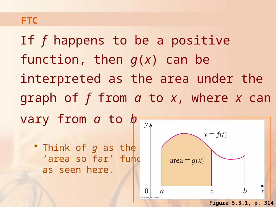
If f happens to be a positive function, then g(x)
can be interpreted as the area under the
graph of f from a to x, where x can vary from a
to b.
Think of g as the ‘area so far’ function, as seen here.
FTC
Figure 5.3.1, p. 314

If f is the function
whose graph is shown
and ,
find the values of:
g(0), g(1), g(2), g(3),
g(4), and g(5).
Then, sketch a rough graph of g.
Example 1
0( ) ( )
xg x f t dt
FTC
Figure 5.3.2, p. 314
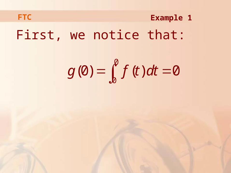
First, we notice that:
0
0(0) ( ) 0g f t dt
FTC Example 1
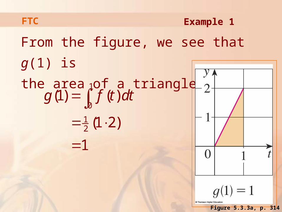
From the figure, we see that g(1) is
the area of a triangle:
1
0
12
(1) ( )
(1 2)
1
g f t dt
Example 1FTC
Figure 5.3.3a, p. 314
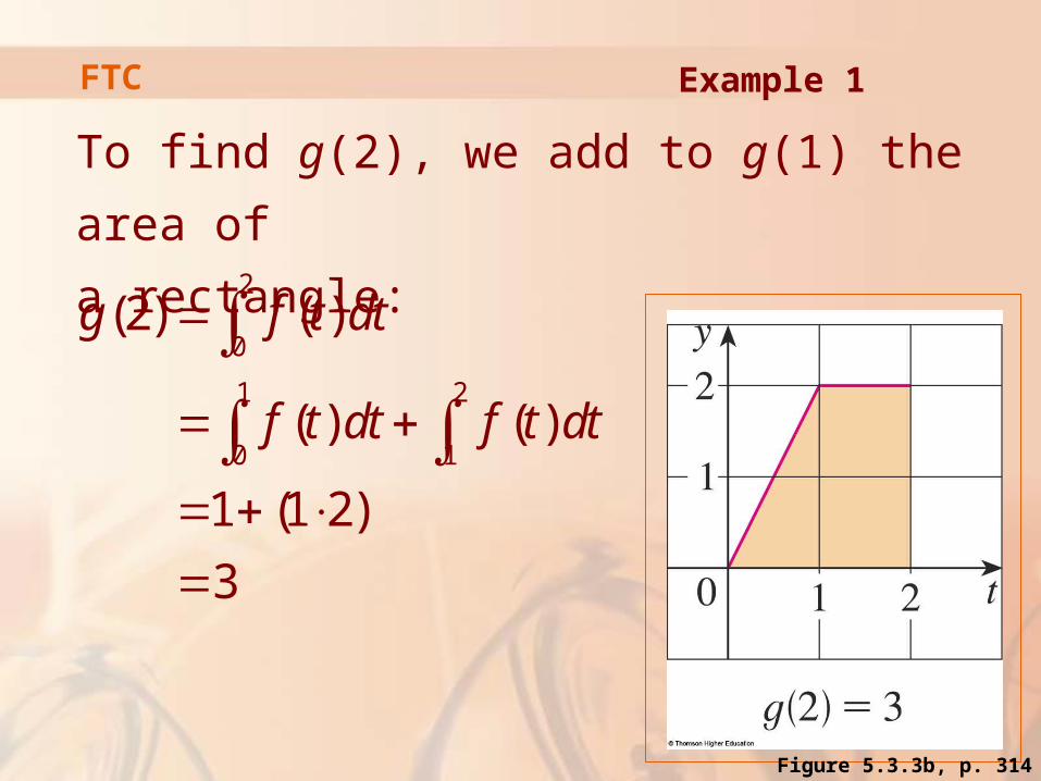
To find g(2), we add to g(1) the area of
a rectangle:2
0
1 2
0 1
(2) ( )
( ) ( )
1 (1 2)
3
g f t dt
f t dt f t dt
Example 1FTC
Figure 5.3.3b, p. 314
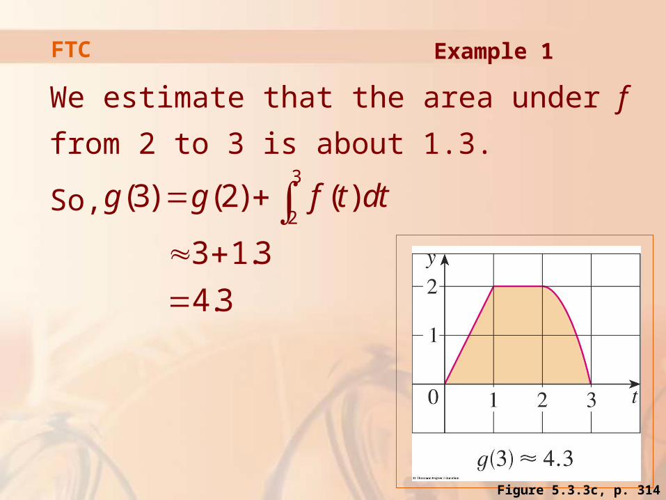
We estimate that the area under f from 2 to 3
is about 1.3.
So, 3
2(3) (2) ( )
3 1.3
4.3
g g f t dt
Example 1FTC
Figure 5.3.3c, p. 314

Thus,4
3(4) (3) ( ) 4.3 ( 1.3) 3.0g g f t dt
FTC Example 1
5
4(5) (4) ( ) 3 ( 1.3) 1.7g g f t dt
Figure 5.3.3d, p. 314 Figure 5.3.3e, p. 314
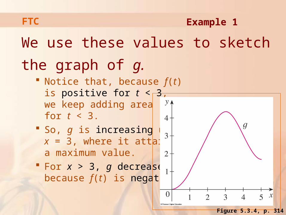
We use these values to sketch the graph
of g. Notice that, because f(t)
is positive for t < 3, we keep adding area for t < 3.
So, g is increasing up to x = 3, where it attains a maximum value.
For x > 3, g decreases because f(t) is negative.
Example 1FTC
Figure 5.3.4, p. 314

If we take f(t) = t and a = 0, then,
using Exercise 27 in Section 5.2,
we have:2
0( )
2
x xg x t dt
FTC

Notice that g’(x) = x, that is, g’ = f.
In other words, if g is defined as the integral of f by Equation 1, g turns out to be an antiderivative of f—at least in this case.
FTC

If we sketch the derivative
of the function g, as in the
first figure, by estimating
slopes of tangents, we get
a graph like that of f in the
second figure.
So, we suspect that g’ = f in Example 1 too.
FTC
Figure 5.3.4, p. 314
Figure 5.3.2, p. 314
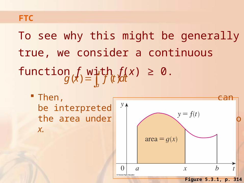
To see why this might be generally true, we
consider a continuous function f with f(x) ≥ 0.
Then, can be interpreted as the area under the graph of f from a to x.
( ) ( )x
ag x f t dt
FTC
Figure 5.3.1, p. 314
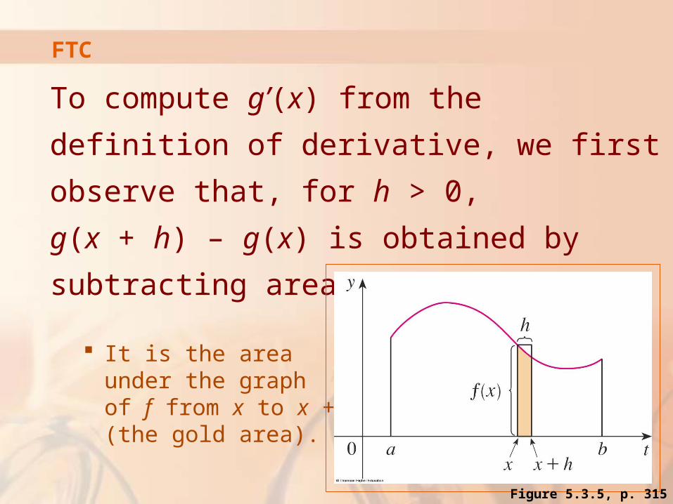
To compute g’(x) from the definition of
derivative, we first observe that, for h > 0,
g(x + h) – g(x) is obtained by subtracting
areas.
It is the area under the graph of f from x to x + h (the gold area).
FTC
Figure 5.3.5, p. 315
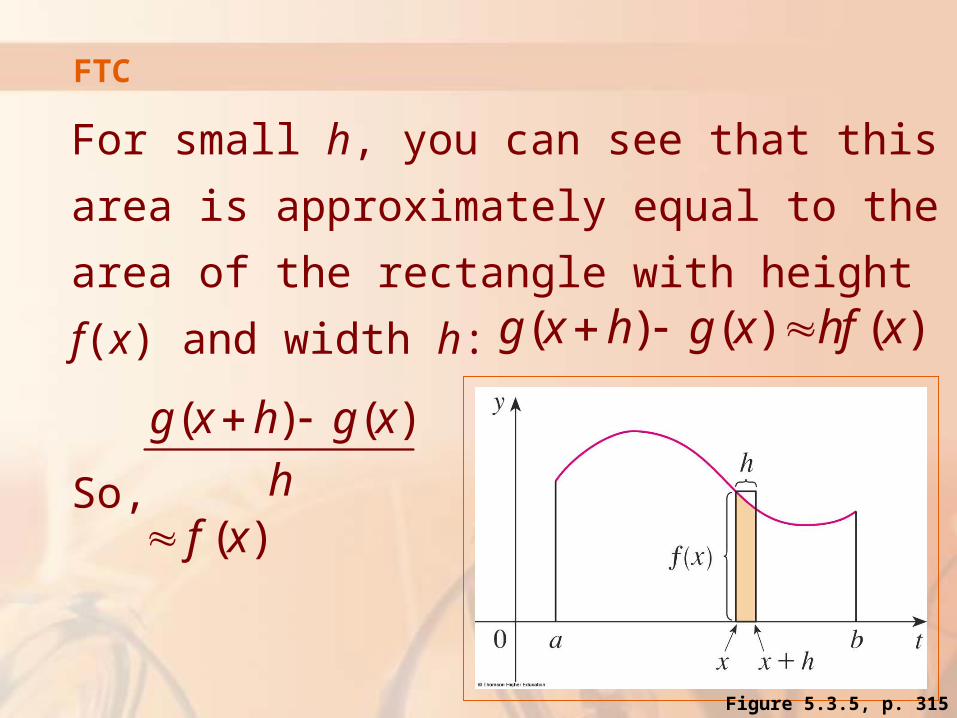
For small h, you can see that this area is
approximately equal to the area of the
rectangle with height f(x) and width h:
So,
FTC
( ) ( ) ( )g x h g x hf x
( ) ( )
( )
g x h g x
hf x
Figure 5.3.5, p. 315

Intuitively, we therefore expect that:
The fact that this is true, even when f is not necessarily positive, is the first part of the FTC (FTC1).
0
( ) ( )'( ) lim ( )
h
g x h g xg x f x
h
FTC
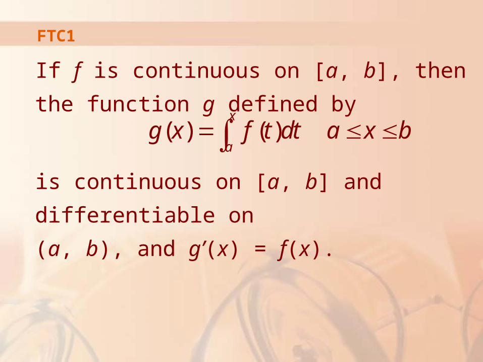
FTC1
If f is continuous on [a, b], then the function g
defined by
is continuous on [a, b] and differentiable on
(a, b), and g’(x) = f(x).
( ) ( )x
ag x f t dt a x b
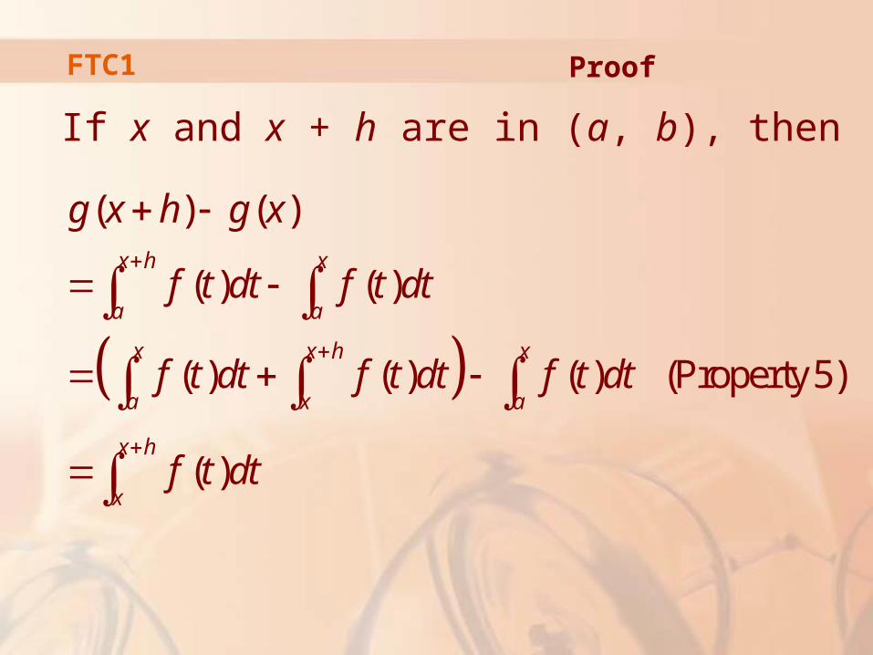
If x and x + h are in (a, b), then
( ) ( )
( ) ( )
( ) ( ) ( ) (Property5)
( )
x h x
a a
x x h x
a x a
x h
x
g x h g x
f t dt f t dt
f t dt f t dt f t dt
f t dt
ProofFTC1
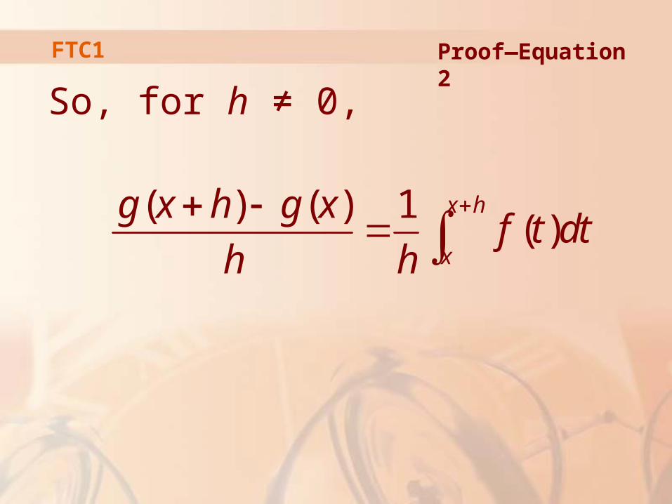
So, for h ≠ 0,
Proof—Equation 2
( ) ( ) 1( )
x h
x
g x h g xf t dt
h h
FTC1
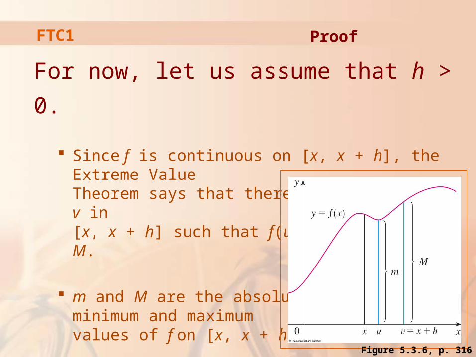
For now, let us assume that h > 0.
Since f is continuous on [x, x + h], the Extreme Value Theorem says that there are numbers u and v in [x, x + h] such that f(u) = m and f(v) = M.
m and M are the absolute minimum and maximum values of f on [x, x + h].
ProofFTC1
Figure 5.3.6, p. 316
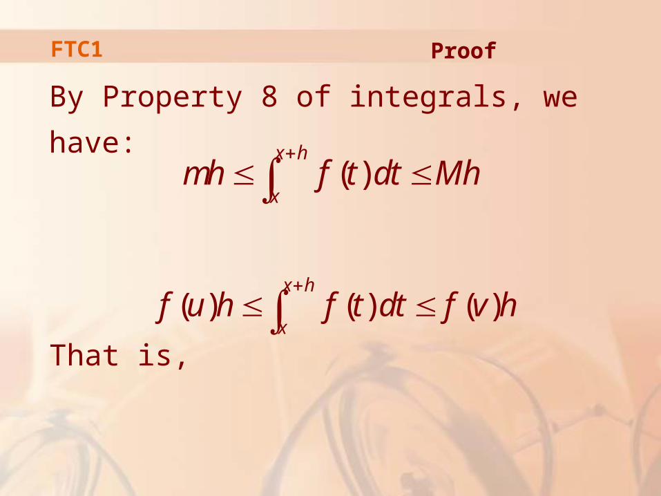
By Property 8 of integrals, we have:
That is,
( )
x h
xmh f t dt Mh
ProofFTC1
( ) ( ) ( )
x h
xf u h f t dt f v h
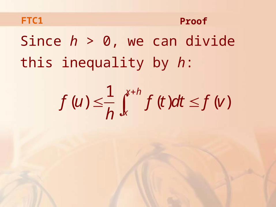
Since h > 0, we can divide this inequality
by h:
1( ) ( ) ( )
x h
xf u f t dt f v
h
FTC1 Proof
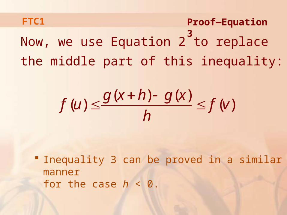
Now, we use Equation 2 to replace the middle
part of this inequality:
Inequality 3 can be proved in a similar manner for the case h < 0.
( ) ( )( ) ( )
g x h g xf u f v
h
Proof—Equation 3FTC1
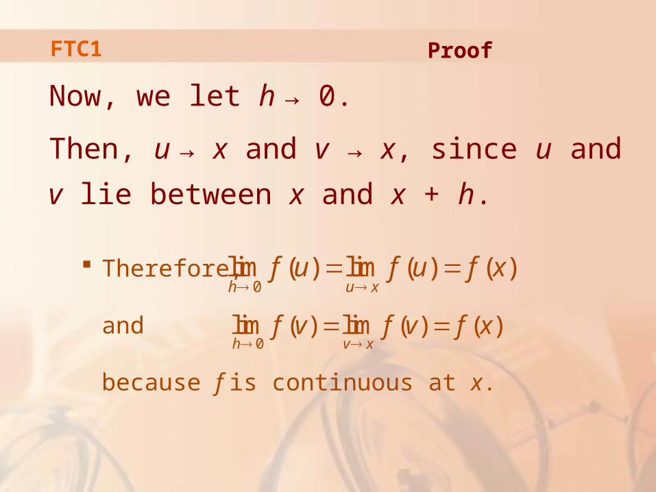
Now, we let h → 0.
Then, u → x and v → x, since u and v lie
between x and x + h.
Therefore,
and
because f is continuous at x.
0lim ( ) lim ( ) ( )h u x
f u f u f x
ProofFTC1
0lim ( ) lim ( ) ( )h v x
f v f v f x
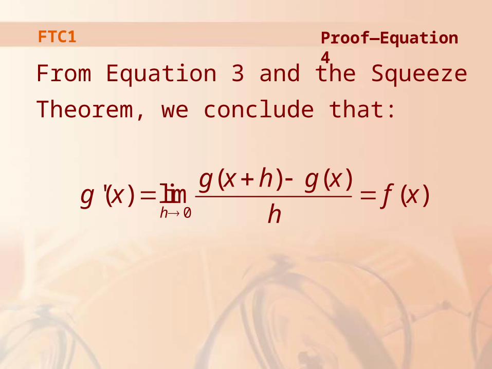
From Equation 3 and the Squeeze
Theorem, we conclude that:
Proof—Equation 4
0
( ) ( )'( ) lim ( )
h
g x h g xg x f x
h
FTC1

Using Leibniz notation for derivatives, we can
write the FTC1 as
when f is continuous.
Roughly speaking, Equation 5 says that, if we first integrate f and then differentiate the result, we get back to the original function f.
( ) ( )x
a
df t dt f x
dx
Equation 5FTC1
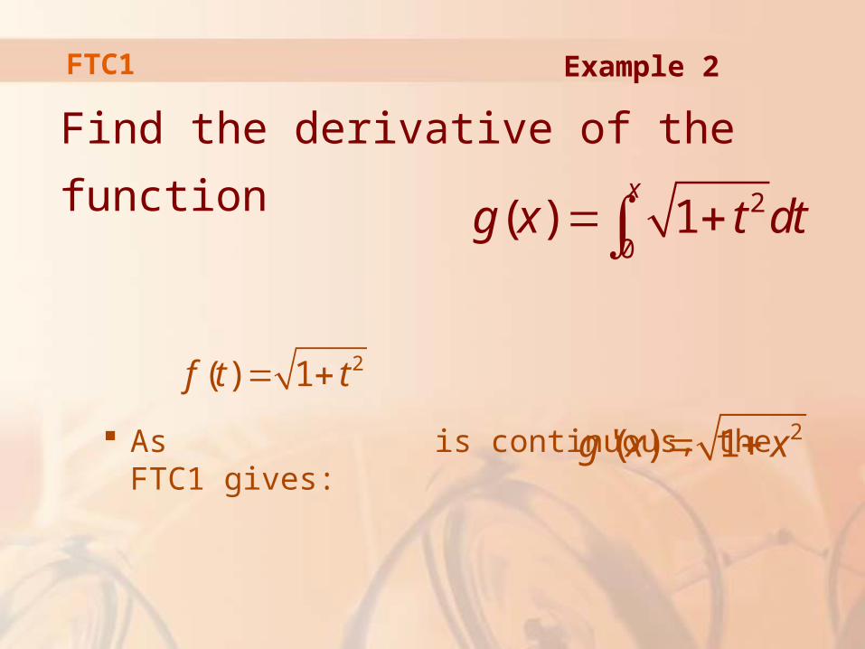
Find the derivative of the function
As is continuous, the FTC1 gives:
Example 2
2
0( ) 1
xg x t dt
2( ) 1f t t 2'( ) 1g x x
FTC1
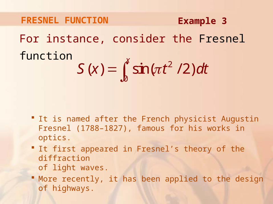
FRESNEL FUNCTION
For instance, consider the Fresnel function
It is named after the French physicist Augustin Fresnel (1788–1827), famous for his works in optics.
It first appeared in Fresnel’s theory of the diffraction of light waves.
More recently, it has been applied to the design of highways.
2
0( ) sin( / 2)
xS x t dt
Example 3
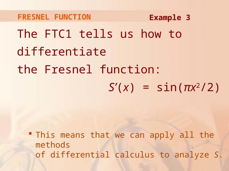
FRESNEL FUNCTION
The FTC1 tells us how to differentiate
the Fresnel function:
S’(x) = sin(πx2/2)
This means that we can apply all the methods of differential calculus to analyze S.
Example 3
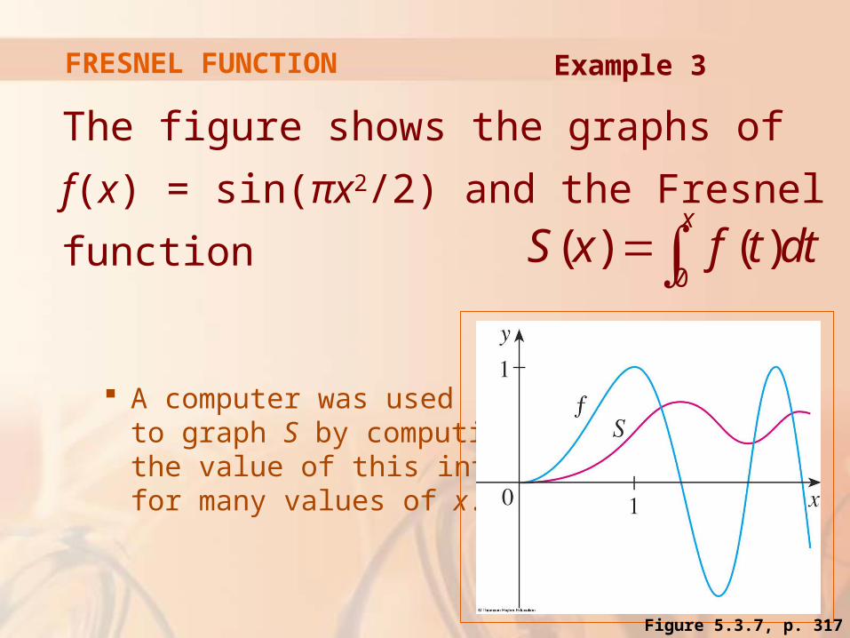
The figure shows the graphs of
f(x) = sin(πx2/2) and the Fresnel function
A computer was used to graph S by computing the value of this integral for many values of x.
0( ) ( )
xS x f t dt
Example 3FRESNEL FUNCTION
Figure 5.3.7, p. 317
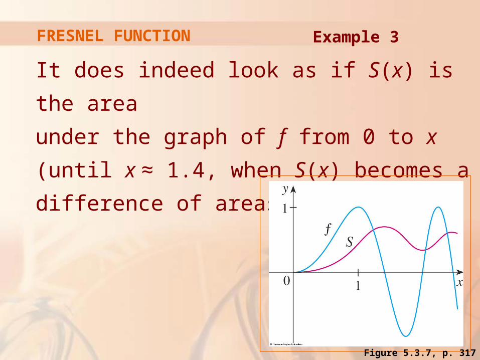
It does indeed look as if S(x) is the area
under the graph of f from 0 to x (until x ≈ 1.4,
when S(x) becomes a difference of areas).
Example 3FRESNEL FUNCTION
Figure 5.3.7, p. 317
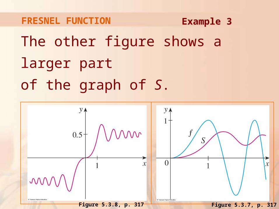
The other figure shows a larger part
of the graph of S.
Example 3FRESNEL FUNCTION
Figure 5.3.7, p. 317Figure 5.3.8, p. 317

If we now start with the graph of S here and
think about what its derivative should look like,
it seems reasonable that S’(x) = f(x).
For instance, S is increasing when f(x) > 0 and decreasing when f(x) < 0.
Example 3FRESNEL FUNCTION
Figure 5.3.7, p. 317
Find
Here, we have to be careful to use the Chain Rule in conjunction with the FTC1.
4
1sec
xdt dt
dx
Example 4FTC1
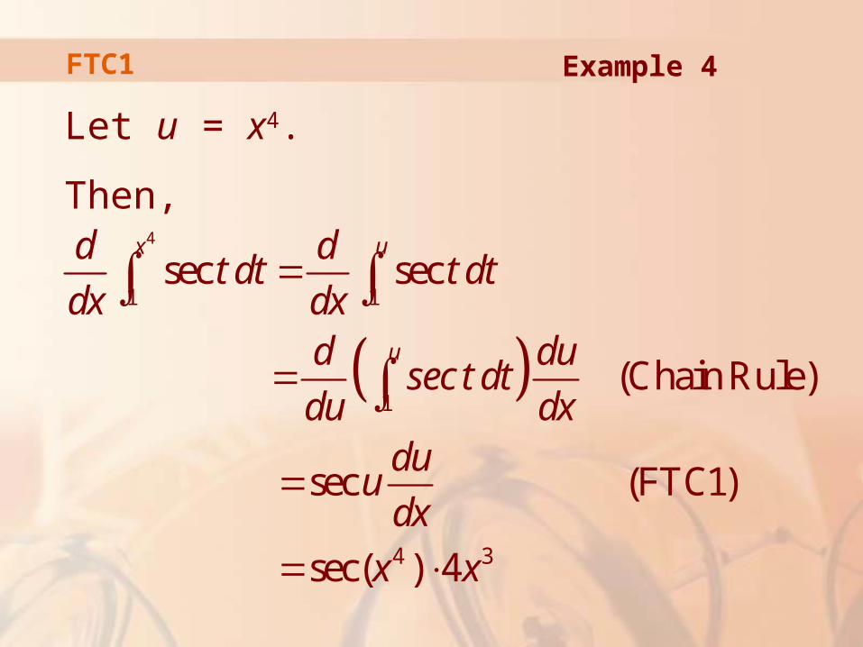
Let u = x4.
Then,
4
1 1
1
4 3
sec sec
(Chain Rule)
sec (FTC1)
sec( ) 4
x u
u
d dt dt t dt
dx dxd du
sec t dtdu dx
duudx
x x
Example 4FTC1
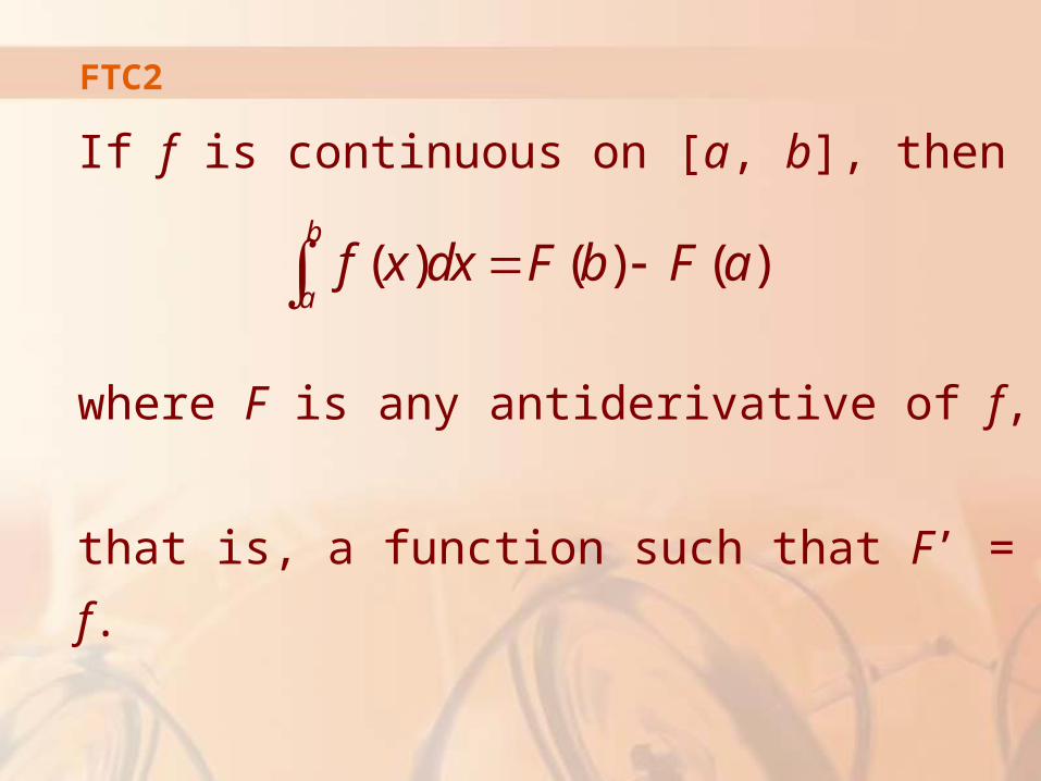
FTC2
If f is continuous on [a, b], then
where F is any antiderivative of f,
that is, a function such that F’ = f.
( ) ( ) ( )b
af x dx F b F a
FTC2
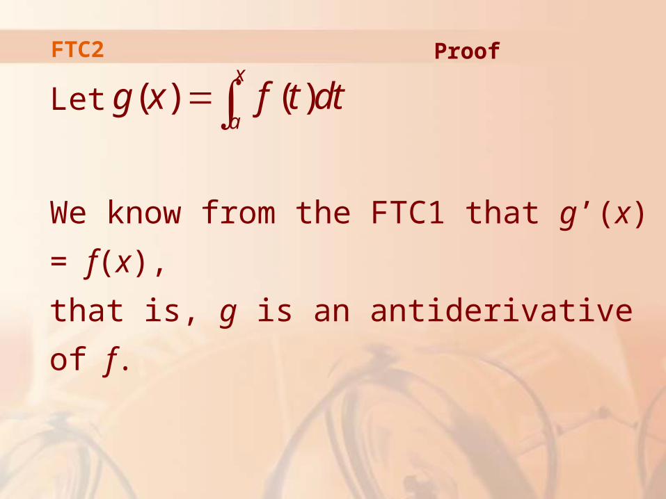
Let
We know from the FTC1 that g’(x) = f(x),
that is, g is an antiderivative of f.
( ) ( )x
ag x f t dt
Proof

FTC2
If F is any other antiderivative of f on [a, b],
then we know from Corollary 7 in Section 4.2
that F and g differ by a constant:
F(x) = g(x) + C
for a < x < b.
Proof—Equation 6
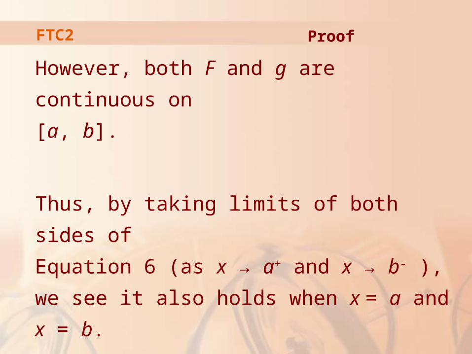
FTC2
However, both F and g are continuous on
[a, b].
Thus, by taking limits of both sides of
Equation 6 (as x → a+ and x → b- ),
we see it also holds when x = a and x = b.
Proof
FTC2
If we put x = a in the formula for g(x),
we get:
Proof
( ) ( ) 0a
ag a f t dt

FTC2
So, using Equation 6 with x = b and x = a,
we have:
( ) ( ) [ ( ) ] [ ( ) ]
( ) ( )
( )
( )b
a
F b F a g b C g a C
g b g a
g b
f t dt
Proof
FTC2
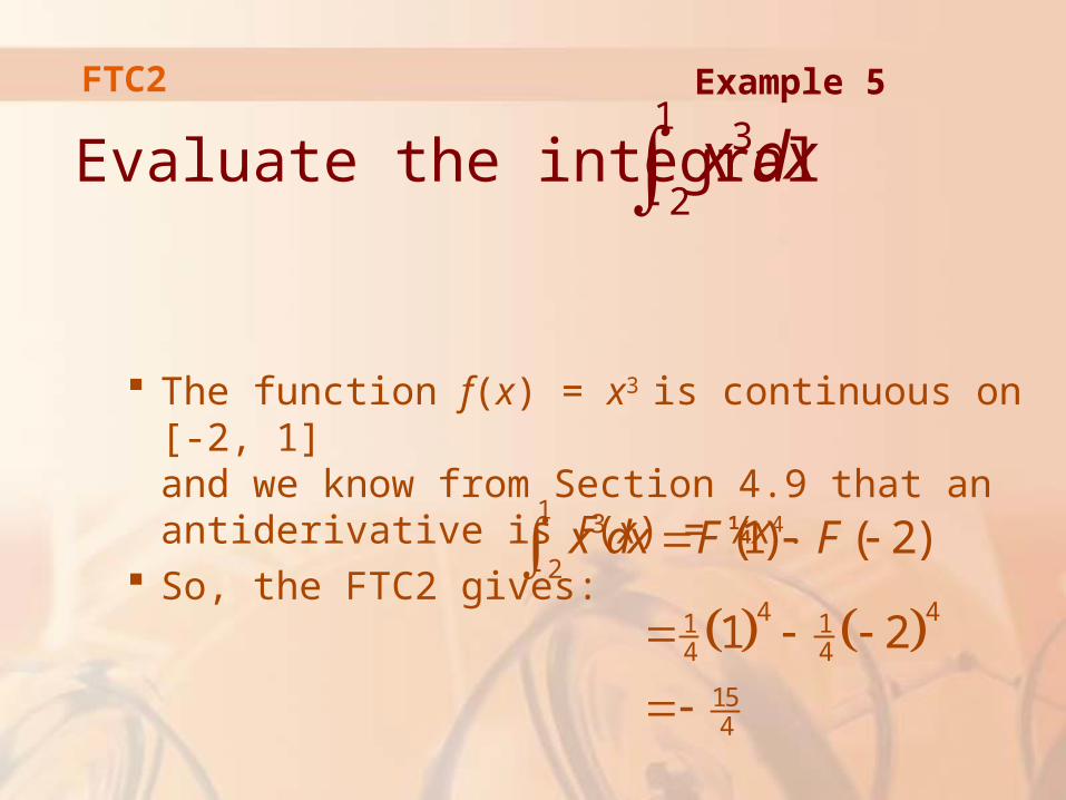
Evaluate the integral
The function f(x) = x3 is continuous on [-2, 1] and we know from Section 4.9 that an antiderivative is F(x) = ¼x4.
So, the FTC2 gives:
Example 51 3
2 x dx
1 3
2
4 41 14 4
154
(1) ( 2)
1 2
x dx F F

FTC2
Notice that the FTC2 says that we can use any antiderivative F of f.
So, we may as well use the simplest one, namely F(x) = ¼x4, instead of ¼x4 + 7 or ¼x4 + C.
Example 5
FTC2
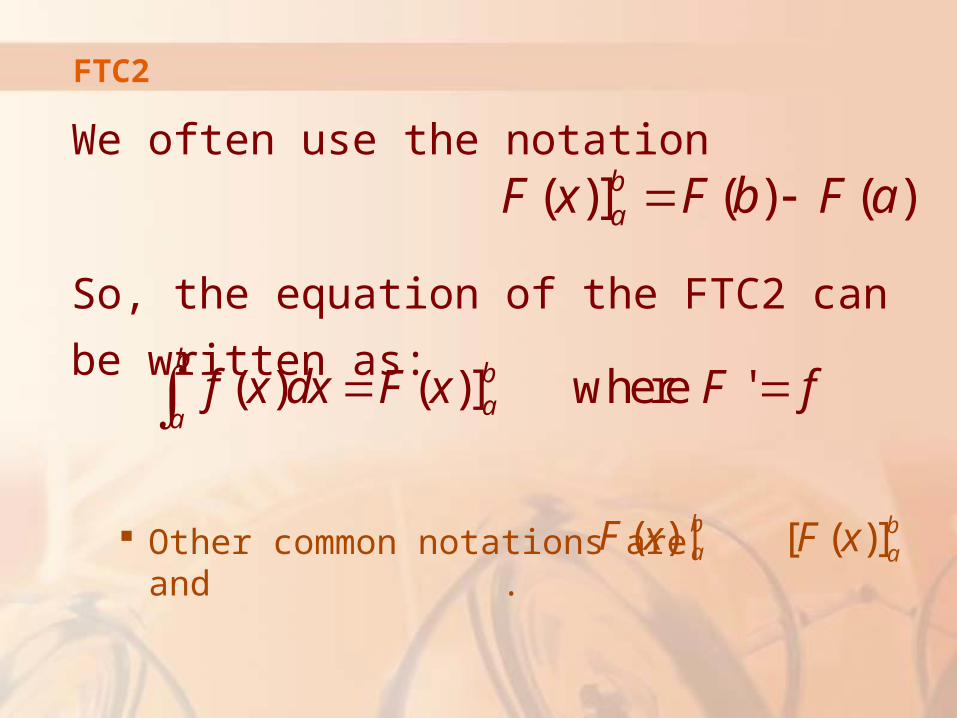
We often use the notation
So, the equation of the FTC2 can be written
as:
Other common notations are and .
( )] ( ) ( )baF x F b F a
( ) ( )] where 'b b
aaf x dx F x F f
( ) |baF x [ ( )]baF x

FTC2
Find the area under the parabola y = x2
from 0 to 1.
An antiderivative of f(x) = x2 is F(x) = (1/3)x3. The required area is found using the FTC2:
Example 6
13 3 31 2
00
1 0 1
3 3 3 3
xA x dx
FTC2
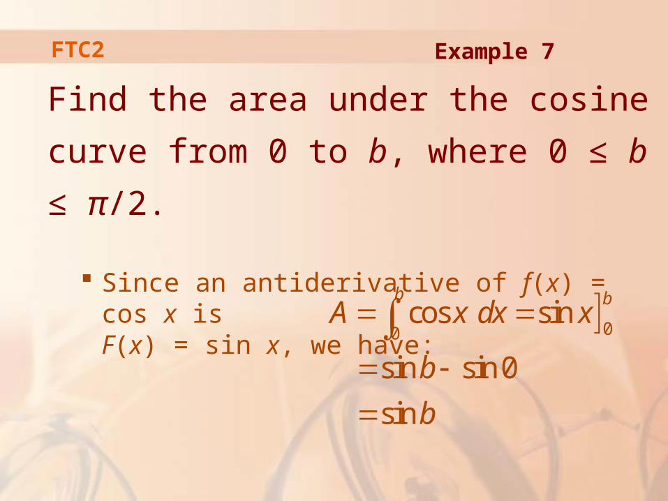
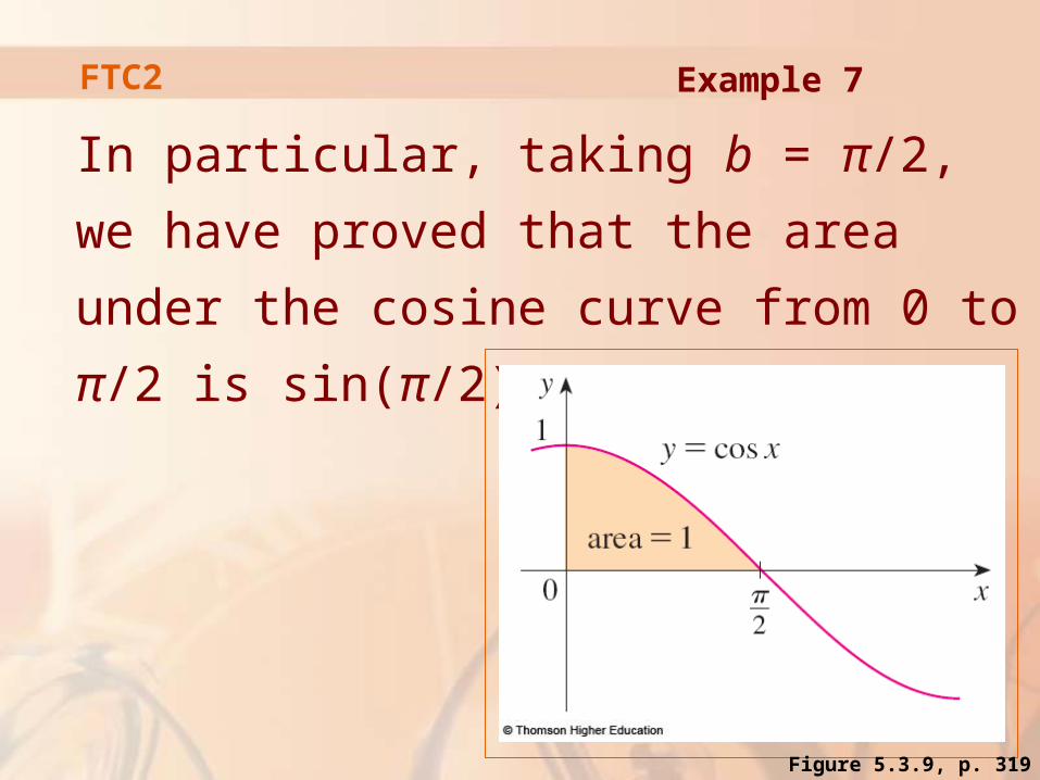
Find the area under the cosine curve
from 0 to b, where 0 ≤ b ≤ π/2.
Since an antiderivative of f(x) = cos x is F(x) = sin x, we have:
Example 7
00cos sin
sin sin 0
sin
b b
A x dx x
b
b
FTC2
In particular, taking b = π/2, we have
proved that the area under the cosine curve
from 0 to π/2 is sin(π/2) =1.
Example 7
Figure 5.3.9, p. 319
FTC2
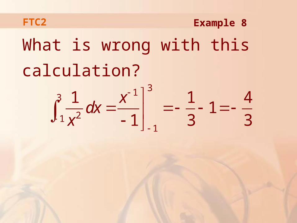
What is wrong with this calculation?
313
211
1 1 41
1 3 3
x
dxx
Example 8

FTC2
To start, we notice that the calculation must
be wrong because the answer is negative
but f(x) = 1/x2 ≥ 0 and Property 6 of integrals
says that when f ≥ 0.( ) 0b
af x dx
Example 9
FTC2
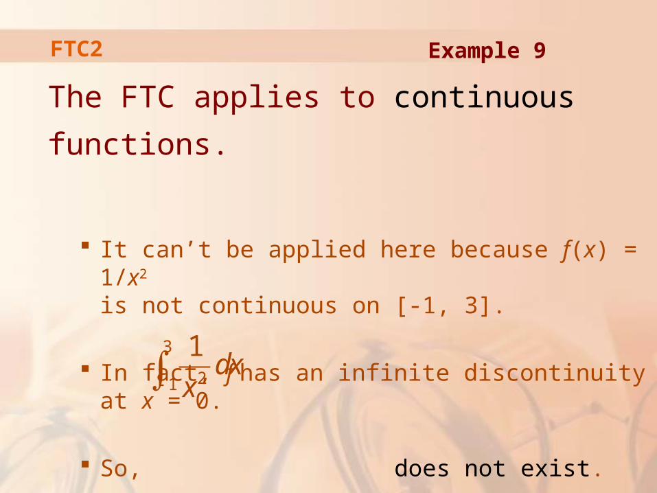
The FTC applies to continuous functions.
It can’t be applied here because f(x) = 1/x2
is not continuous on [-1, 3].
In fact, f has an infinite discontinuity at x = 0.
So, does not exist.3
21
1dx
x
Example 9

FTC
Suppose f is continuous on [a, b].
1.If , then g’(x) = f(x).
2. , where F is
any antiderivative of f, that is, F’ = f.
( ) ( )x
ag x f t dt
( ) ( ) ( )b
af x dx F b F a

INVERSE PROCESSES
We noted that the FTC1 can be rewritten
as:
This says that, if f is integrated and then the result is differentiated, we arrive back at the original function f.
( ) ( )x
a
df t dt f x
dx
INVERSE PROCESSES
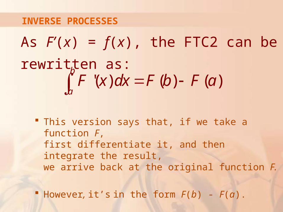
As F’(x) = f(x), the FTC2 can be rewritten
as:
This version says that, if we take a function F, first differentiate it, and then integrate the result, we arrive back at the original function F.
However, it’s in the form F(b) - F(a).
'( ) ( ) ( )b
aF x dx F b F a

SUMMARY
Before it was discovered—from the time
of Eudoxus and Archimedes to that of Galileo
and Fermat—problems of finding areas,
volumes, and lengths of curves were so
difficult that only a genius could meet
the challenge.
SUMMARY
Now, armed with the systematic method
that Newton and Leibniz fashioned out of
the theorem, we will see in the chapters to
come that these challenging problems are
accessible to all of us.
Recommended