Input, Representation, and Access Pattern GuidedCache Locality Optimizations for Graph Analytics
Submitted in partial fulfillment of the requirements for
the degree of
Doctor of Philosophy
in
Electrical and Computer Engineering
Vignesh Balaji
B.E., Electronics and Instrumentation, BITS PilaniM.S., Electrical and Computer Engineering, Carnegie Mellon University
Carnegie Mellon UniversityPittsburgh, PA
August 2021

c©Vignesh Balaji, 2021All Rights Reserved

Acknowledgements
So many people have helped me get to this stage of my PhD and I would like to offer my most sincere thanks
to everyone who has contributed along the way. First, I want to thank my advisor, Brandon Lucia. Brandon
has been a caring mentor and he has been deeply invested in improving my research skills. Most of what I
know about asking the right questions in research, giving effective presentations, and writing with clarity, I
learned from Brandon. Besides developing my research skills, Brandon has also been a passionate advocate
for my career growth by actively creating opportunities for me to participate in program committees, attend
conferences, and go for internships. I am also thankful to Brandon for his patience and support, especially
during the initial years of my PhD when I struggled to find traction with my research. His support during this
crucial period of my PhD really means a lot to me. I am deeply grateful to Brandon for shaping me to be the
researcher that I am today.
I would also like to thank my thesis committee members – Aamer Jaleel, Nathan Beckmann, and James
Hoe – for all their guidance and help in improving the quality of my work. Aamer Jaleel has been a
wonderful mentor and collaborator. As my internship mentor, Aamer made sure that I had a rewarding and
fun experience at NVIDIA and he really made me feel at home in Westford. As a collaborator on the P-OPT
project, Aamer helped me every step of the way, from honing the initial idea to getting the paper ready for
submission. I am especially grateful to Aamer for all the help and advice he offered during my job search; it
really helped reduce the stress associated with job search. I could not be more excited at the prospect of being
able to continue our collaboration during the next phase of my career. As the caching and graph analytics
expert, Nathan Beckmann’s pointed critiques of my work helped strengthen many of my submissions. I
would also like to thank Nathan for his idea of setting up group meetings where everyone provides a short
summary of papers accepted in recent conferences. These group meetings have been a great way to get a
gist of all the papers presented in each architecture conference. James Hoe encouraged me to think more
broadly about the larger context of my work and his advice has helped me motivate my work better. I am
also thankful to James Hoe for arranging interesting speakers for the CALCM seminars. I have learned a lot
about computer architecture from attending these seminars. Beyond my thesis committee, I would also like
to thank Mike Bond and his students (Rui Zhang and Swarnendu Biswas) for being early collaborators and
sparking my interest in memory consistency models and cache coherence. Thanks also to Radu Marculescu
for co-advising me during the initial years of my PhD. Finally, I would like to thank Diana Marculescu and
Onur Multu for being my initial points of contact at CMU and playing an important role in getting me to
CMU in the first place.
iii

iv
I was fortunate to go for internships at NVIDIA and Intel during my PhD and both my internships were
deeply transformational experiences. My interactions with NVIDIA’s Architecture Research Group members
at Westford (Joel Emer, Aamer Jaleel, Neal Crago, Michael Pellauer, and Angshuman Parashar) taught me
the value of building analytical models for studying architecture problems (a skill that I have used throughout
the rest of my PhD). I would also like to thank the other interns (Hyoukjun Kwon, Mengjia Yan, Victor Ying,
and Thomas Bourgeat) for being terrific collaborators during the internship. The NVIDIA internship was also
very important because it spawned a long and fruitful collaboration with Aamer Jaleel and Neal Crago. The
P-OPT project took quite some time to go from conception to submission and I am thankful to Aamer and
Neal for their patience and support over the course of the project. Thanks also to Hailang Liou for his early
experiments that later informed the core design of P-OPT. My internship at Intel’s Parallel Computing Lab
gave me the opportunity to apply the learnings of graph analytics to a new problem domain – sparse tensor
algebra. I am very grateful to Shaden Smith for being an excellent mentor during my stint at Intel. Shaden
helped me on so many fronts, from teaching me about sparse tensor workloads to giving career advice to
introducing me to researchers within Intel. I would also like to thank Fabrizio Petrini for extending me an
internship offer even though I was a bit late in the game and to Christopher Hughes who put in a good word
for me after we interacted at IISWC 2018. I must also thank my friends – Eshan Bhatia, Abhishek Mahajan,
and Ishan Tyagi – for making my internship summers very fun and memorable experiences.
I have had the good fortune of having an amazing set of colleagues at CMU. I would like to thank
all the members of the ABSTRACT research group (Alexei Colin, Emily Ruppel, Kiwan Maeng, Graham
Gobieski, Milijana Surbatovich, Brad Denby, Harsh Desai, McKenzie van der Hagen, and Nathan Serafin). I
am grateful for the feedback they have provided for all my practice talks and for their help in refining my
presentations. I have also thoroughly enjoyed being conference buddies and getting to explore different
cities with them post-conference. Special thanks to the early members of ABSTRACT (Alexei Colin, Kiwan
Maeng, and Emily Ruppel) for being such inspiring colleagues during the initial years of my PhD when I
still figuring out research. Alexei Colin set a high bar for what a PhD thesis could accomplish and showed
me the importance of pursuing research aimed at broad adoption. Kiwan Maeng has showed me the value of
not being afraid to seek help in order to make quick progress on a broad range of topics. Emily Ruppel has
taught me the value of being an enthusiastic team player in pursuing large and interesting projects. I would
also like to thank members of the CORGi research group (Brian Schwedock, Elliot Lockermann, and Sara
McAllister) for the entertaining lunch group discussions. As a young PhD student, I greatly benefited from
the sage advice offered by early denizens of CIC 4th floor – Nandita Vijaykumar, Rachata Ausavarungnirun,
Saugata Ghose, Chris Fallin, Kevin Hsieh, and Utsav Drolia – and I thank them for their advice. I have
also had the opportunity to interact with many PhD students through reading groups, courses, and EGO
mixers – Pratik Fegade, Sandeep D’souza, Sanghamitra Dutta, Dimitrios Stamoulis, Antonis Manousis, Joe
Sweeney, Shunsuke Aoki, Amirali Boroumand, Ankur Mallick, and Mark Blanco – and I thank them all for
our commiserations on the PhD experience. Finally, I would like to offer my thanks to the administrative
staff (Holly Skovira and Grace Bintrim) for making reimbursements painless, to Jeanine for her cheerful
conversations, and to the CMU shuttle drivers for their vitally important role in supporting my nocturnal
lifestyle.

v
My stay in Pittsburgh would not have been nearly as much fun or productive without my friends. Minesh
Patel was one of the first few friends I made in Pittsburgh and he really helped me feel comfortable during
the initial days while I was still learning to be a PhD student in a foreign land. During the advisor selection
period, it was Minesh who suggested that I go meet with Brandon and I am grateful to Minesh for making
that suggestion. Prashanth Mohan has been friend from the very beginning and we have teamed up on so
many things over the years ranging from the mundane (figuring out how to file our first tax returns) to the
adventurous (exploring bike trails during the summer). I am also thankful to Prashanth for facilitating my
very brief foray into Advaita Vedanta. I would also like to thank Kartikeya Bhardwaj and Susnata Mondal for
their camaradarie over the years and for the fun experiences over dinners and movies. I am very glad that
Mukul Bhutani joined CMU during my fourth year at CMU. Mukul has been a close friend from the early
days of my undergraduate degree and it was so great to be able to reconnect again in a different continent.
The wide-ranging discussions over dinners with Mukul were a welcome break from research. Thanks also
to my ECE batchmate Rajat Kateja. Rajat and I joined the department in the same year and we seem to
have followed a very similar trajectory (from wanting to go to academia at the beginning of our PhDs to
deciding to switch to a different career path at the same point). It was always comforting to have someone
with such a remarkably similar vision. Thanks also to Abhilasha Jain and Samarth Gupta for taking me on
an amazing star-gazing trip in West Virginia. Finally, I want to thank my first-year flatmates Guruprasad
Raghavan, Anchit Sood, and Prem Solanki for helping me figure out life in Pittsburgh.
Going further back, I must also acknowledge the important role played by my undergraduate experiences
in shaping my research career. My interactions with the members of IBM’s Semiconductor Research
and Development Center, particularly with Samarth Agarwal and Suresh Gundapaneni, were pivotal in
finalizing my decision to pursue a PhD. I got my first exposure to computer architecture research during my
undergraduate thesis in S. K. Nandy’s lab at IISc and I would like to thank the members of his research group
for showing me the ropes. Thanks to Balasubramaniam Srinivasan for introducing me to S. K. Nandy and
encouraging me to tag along on the thesis project. I would like to offer special thanks to Eshan Bhatia for
collaborating on almost every project during our undergraduate days. I am sure these early collaborations
played a significant role in developing my interest towards computer architecture research.
Finally, I need to thank the most important people who made this thesis work possible – my parents
(Nagarajan Balaji and Annapurani Balaji). My parents offered me complete freedom to chart my own course
and have whole-heartedly supported my every decision. From a very early age, they instilled in me the value
of hard work and dedication without which I would not have been able to reach this point. For being there
with me through all the highs and lows of my PhD, for listening to all my practice talks, for proofreading
almost every piece of writing that I produced during my PhD (including this one), this thesis belongs to my
parents as much as it does to me.
The thesis projects were supported in part by National Science Foundation grant XPS-1629196 and the Intel Science andTechnology Center for Visual Cloud Systems (ISTC-VCS)

Dedicated to Amma and Appa

Abstract
Graph analytics has many important commercial and scientific applications ranging from social network
analysis to tracking disease transmission using contact networks. Early works in graph analytics primarily
focused on processing graphs using large-scale distributed systems. More recently, increasing main memory
capacities and core counts have prompted a shift towards analyzing large graphs using just a single machine.
Multiple studies have demonstrated that in-memory graph analytics can even outperform distributed graph
analytics. However, performance of in-memory graph analytics is still far from optimal because the charac-
teristic irregular memory access pattern of graph applications leads to poor cache locality. Irregular memory
accesses are fundamental to graph analytics and are a product of the sparsity pattern of input graphs and the
compressed representation used to store graphs. The main insight of this thesis is that the different sources of
irregularity in graph analytics also contain valuable information that can be used to design cache locality
optimizations. Using this insight, we propose three types of optimizations that each leverage properties
of input graphs, compressed representations, and application access patterns to improve locality of graph
analytics workloads.
First, we present Selective Graph Reordering and RADAR which are cache locality optimizations that
leverage the structural properties of input graphs. Graph reordering uses a graph’s structure to improve the
data layout for graph application data in a bid to improve locality. However, when accounting for overheads,
graph reordering offers questionable benefits; providing speedups for some graphs while causing a net
slowdown in others. To improve the viability of graph reordering, we develop a low-overhead analytical
model to accurately predict the performance improvement from reordering. Our analytical model allows
selective application of graph reordering only for the graphs which are expected to receive high speedups
while avoiding slowdowns for other graphs. RADAR builds upon graph reordering to perform memory-
efficient data duplication for power-law graphs to eliminate expensive atomic updates. Combining graph
reordering with data duplication allows RADAR to simultaneously optimize cache locality and scalability of
parallel graph applications.
Second, we present P-OPT, an optimized cache replacement policy that leverages the popular compressed
representation used in graph analytics – CSR and CSC – to improve locality for graph applications. Our work
is based on the observation that the CSR and CSC efficiently encode information about future accesses of
graph application data, enabling Belady’s optimal cache replacement policy (an oracular policy that represents
the theoretical upper bound in cache replacement). P-OPT is a practical implementation of Belady’s optimal
replacement policy. By using the graph structure to guide near-optimal cache replacement, P-OPT is able to
vii

viii
significantly reduce cache misses compared to heuristics-based, state-of-the-art replacement policies.
Finally, we present HARP, a hardware-based cache locality optimization that leverages the typical
access pattern of graph analytics workloads. HARP builds upon Propagation Blocking, a software cache
locality optimization targeting applications with irregular memory updates. Due to the pervasiveness of the
irregular memory updates, Propagation Blocking applies to a broader range of workloads beyond just graph
analytics. HARP provides architecture support for Propagation Blocking to eliminate the lingering sources of
inefficiency in a Propagation Blocking execution, allowing HARP to further improve the performance gains
from Propagation Blocking for graph analytics and other irregular memory workloads.
Contents
Acknowledgements iii
Abstract vii
List of Tables xi
List of Figures xiii
1 Introduction 1
1.1 Graph Analytics has Important Applications . . . . . . . . . . . . . . . . . . . . . . . . . . 1
1.2 The Case for In-memory Graph Analytics . . . . . . . . . . . . . . . . . . . . . . . . . . . 2
1.3 The Primary Bottleneck of In-memory Graph Analytics: Poor Locality . . . . . . . . . . . . 5
1.4 Factors Affecting Cache Locality of Graph Analytics . . . . . . . . . . . . . . . . . . . . . 6
1.5 Outline of Thesis Contributions . . . . . . . . . . . . . . . . . . . . . . . . . . . . . . . . . 11
2 Predicting Graph Reordering Speedups with Packing Factor 15
2.1 The Case for Lightweight Graph Reordering . . . . . . . . . . . . . . . . . . . . . . . . . . 16
2.2 Performance Improvements from Lightweight Graph Reordering . . . . . . . . . . . . . . . 17
2.3 When is Lightweight Reordering a Suitable Optimization? . . . . . . . . . . . . . . . . . . 27
2.4 Selective Lightweight Graph Reordering Using the Packing Factor . . . . . . . . . . . . . . 28
2.5 Related Work . . . . . . . . . . . . . . . . . . . . . . . . . . . . . . . . . . . . . . . . . . 32
2.6 Discussion . . . . . . . . . . . . . . . . . . . . . . . . . . . . . . . . . . . . . . . . . . . . 34
3 Improving Locality and Scalability with RADAR 37
3.1 The Case for Combining Duplication and Reordering . . . . . . . . . . . . . . . . . . . . . 38
ix

CONTENTS x
3.2 RADAR: Combining Data Duplication and Graph Reordering . . . . . . . . . . . . . . . . 42
3.3 Performance Improvements with RADAR . . . . . . . . . . . . . . . . . . . . . . . . . . . 47
3.4 Advantages of Using RADAR Compared to Push-Pull . . . . . . . . . . . . . . . . . . . . 52
3.5 Related Work . . . . . . . . . . . . . . . . . . . . . . . . . . . . . . . . . . . . . . . . . . 57
3.6 Discussion . . . . . . . . . . . . . . . . . . . . . . . . . . . . . . . . . . . . . . . . . . . . 59
4 Practical Optimal Cache Replacement for Graph Analytics 61
4.1 Limitations of Existing Cache Replacement Policies . . . . . . . . . . . . . . . . . . . . . . 62
4.2 Transpose-Directed Belady’s Optimal Cache replacement . . . . . . . . . . . . . . . . . . . 63
4.3 P-OPT: Practical Optimal Cache Replacement . . . . . . . . . . . . . . . . . . . . . . . . . 66
4.4 P-OPT Architecture . . . . . . . . . . . . . . . . . . . . . . . . . . . . . . . . . . . . . . . 70
4.5 Cache Locality Improvements with P-OPT . . . . . . . . . . . . . . . . . . . . . . . . . . . 77
4.6 Related Work . . . . . . . . . . . . . . . . . . . . . . . . . . . . . . . . . . . . . . . . . . 84
4.7 Discussion . . . . . . . . . . . . . . . . . . . . . . . . . . . . . . . . . . . . . . . . . . . . 85
5 Generalizing Beyond Graph Analytics with HARP 87
5.1 Pervasiveness of Irregular Memory Updates . . . . . . . . . . . . . . . . . . . . . . . . . . 88
5.2 Versatility of Propagation Blocking . . . . . . . . . . . . . . . . . . . . . . . . . . . . . . . 89
5.3 Optimizing Propagation Blocking with HARP . . . . . . . . . . . . . . . . . . . . . . . . . 94
5.4 Architecture Support for HARP . . . . . . . . . . . . . . . . . . . . . . . . . . . . . . . . 97
5.5 Performance Improvements with HARP . . . . . . . . . . . . . . . . . . . . . . . . . . . . 103
5.6 Related Work . . . . . . . . . . . . . . . . . . . . . . . . . . . . . . . . . . . . . . . . . . 113
5.7 Discussion . . . . . . . . . . . . . . . . . . . . . . . . . . . . . . . . . . . . . . . . . . . . 114
6 Conclusions 116
6.1 Cross-cutting Themes . . . . . . . . . . . . . . . . . . . . . . . . . . . . . . . . . . . . . . 116
6.2 Future Research Directions . . . . . . . . . . . . . . . . . . . . . . . . . . . . . . . . . . . 118
6.3 Final Remarks . . . . . . . . . . . . . . . . . . . . . . . . . . . . . . . . . . . . . . . . . . 120
Bibliography 121

List of Tables
1.1 Cache locality optimizations proposed in this thesis . . . . . . . . . . . . . . . . . . . . . . 14
2.1 Reordering overhead of Gorder: Gorder improves performance but with extreme overhead. . . 17
2.2 Statistics for the evaluated input graphs: The size of vertex data for all the graphs exceeds
the LLC capacity. . . . . . . . . . . . . . . . . . . . . . . . . . . . . . . . . . . . . . . . . . . 22
2.3 Average percentage of edges processed by Ligra applications: A higher average percentage
of edges processed corresponds to greater reuse in vertex data accesses. The AVG field for each
application represents the average value of the metric across 8 input graphs. . . . . . . . . . . 24
2.4 Impact of LWR on iterations until convergence: Values greater than 1 indicate delayed
convergence compared to baseline execution on the original graph. Values less than 1 indicate
that the execution on the reordered graphs converged in fewer iterations than the execution on
the original graph. . . . . . . . . . . . . . . . . . . . . . . . . . . . . . . . . . . . . . . . . . 26
2.5 Speedups from LWR for push-pull implementations: LWR techniques provide greater
performance improvements for applications that perform pull-style accesses while processing
large frontiers. . . . . . . . . . . . . . . . . . . . . . . . . . . . . . . . . . . . . . . . . . . . 27
3.1 Summary of optimizations: RADAR combines the benefits of Degree Sorting and HUBDUP
while eliminating the overheads of each . . . . . . . . . . . . . . . . . . . . . . . . . . . . . . 42
3.2 Statistics for the evaluated input graphs . . . . . . . . . . . . . . . . . . . . . . . . . . . . . 49
3.3 Number of unique words in the hMask bitvector containing hub vertices: HUBDUP offers
the highest speedups for graphs in which hubs map to the fewest number of unique words in the
bitvector. . . . . . . . . . . . . . . . . . . . . . . . . . . . . . . . . . . . . . . . . . . . . . . 50
xi
List of Tables xii
3.4 Preprocessing costs for HUBDUP, RADAR, and Push-Pull: Degree Sorting and RADAR
have a smaller preprocessing cost compared to Push-Pull. (V - #vertices and E - #edges) . . . 56
4.1 Simulation parameters . . . . . . . . . . . . . . . . . . . . . . . . . . . . . . . . . . . . . . 78
4.2 Applications . . . . . . . . . . . . . . . . . . . . . . . . . . . . . . . . . . . . . . . . . . . . 78
4.3 Input Graphs: All graphs exceed the LLC size. . . . . . . . . . . . . . . . . . . . . . . . . . . 79
4.4 Relative preprocessing cost for P-OPT . . . . . . . . . . . . . . . . . . . . . . . . . . . . . 84
5.1 PB execution breakup: Binning dominates a PB execution both when using a medium no. of
bins (which offers the best overall PB performance) and when using a large no. of bins (which
offers the best Accumulate performance). . . . . . . . . . . . . . . . . . . . . . . . . . . . . . 94
5.2 Simulation parameters . . . . . . . . . . . . . . . . . . . . . . . . . . . . . . . . . . . . . . 104
5.3 Input Graphs and Matrices . . . . . . . . . . . . . . . . . . . . . . . . . . . . . . . . . . . 105

List of Figures
1.1 Locality of graph analytics workloads: Graph applications exhibit a poor LLC hit rate. . . . . 5
1.2 Popular Graph Representations: CSR/CSC are the most memory-efficient data structures for
storing graphs . . . . . . . . . . . . . . . . . . . . . . . . . . . . . . . . . . . . . . . . . . . 7
1.3 Comparison of different graph representations: Operating on CSR (and CSC) is more effi-
cient than COO even after accounting for the preprocessing cost of building the CSR/CSC from
the COO (shaded portion). . . . . . . . . . . . . . . . . . . . . . . . . . . . . . . . . . . . . . 8
1.4 Roofline plot for graph analytics workloads: Graph applications are memory-bound and have
poor DRAM bandwidth utilization. . . . . . . . . . . . . . . . . . . . . . . . . . . . . . . . . 10
1.5 Cache locality from different vertex orders: Changing vertex data layout based on structural
properties of real-world inputs can increase reuse in on-chip caches. . . . . . . . . . . . . . . 12
2.1 Vertex ID assignments generated by different reordering techniques: Vertex IDs are shown
below the degree of the vertex. Highly connected (hub) vertices have been highlighted. Degree
Sorting is only shown for instructive purposes . . . . . . . . . . . . . . . . . . . . . . . . . . . 19
2.2 Speedup after lightweight reordering: Data are normalized to run time with the original vertex
ordering. The total bar height is speedup without accounting for the overhead of lightweight
reordering. The upper, hashed part of the bar represents the overhead imposed by lightweight
reordering. The filled, lower bar segment is the net performance improvement accounting for
overhead. The benchmark suites are differentiated using a suffix (G/L). . . . . . . . . . . . . . . 23
xiii
List of Figures xiv
2.3 Vertex orders of a symmetric bipartite graph by Hub Sorting and Hub Clustering: The
two colors represent the parts of the bipartite graph. Hub Sorting produces a vertex order
wherein vertices from different parts are assigned consecutive vertex IDs whereas Hub Clustering
produces an ordering where vertices belonging to the same part are often assigned consecutive
IDs. . . . . . . . . . . . . . . . . . . . . . . . . . . . . . . . . . . . . . . . . . . . . . . . . . 25
2.4 Relation between speedup from Hub Sorting and packing factor of input graph: Each
point is a speedup of an application executing on Hub Sorted graph compared to the original
graph. Different applications are indicated with different colors/markers. Hub Sorting provides
significant speedup for executions on graphs with high Packing Factor. . . . . . . . . . . . . . 30
2.5 Reduction in LLC and DTLB misses due to Hub Sorting: Hub Sorting provides greater
reduction in LLC misses and DTLB load misses for graphs with high Packing Factor. . . . . . . 31
2.6 End-to-end speedup from selective Hub Sorting: Input graphs have been arranged in increas-
ing order of Packing Factor. Selective application of Hub Sorting based on Packing Factor
provides significant speedups on graphs with high Packing Factor while avoiding slowdowns on
graphs with low Packing Factor. . . . . . . . . . . . . . . . . . . . . . . . . . . . . . . . . . . 32
2.7 Generalizability of the Packing Factor metric: (a) Packing Factor is able to accurately
predict reordering benefits for non-power-law graphs (b) Packing Factor requires modifications
to accurately predict reordering benefits for community-structure based reordering schemes . . 35
3.1 Performance improvement from removing atomic updates in graph applications . . . . . . 39
3.2 False sharing caused by Degree Sorting: Reordering improves performance of a single-
threaded execution but fails to provide speedups for parallel executions. . . . . . . . . . . . . . 41
3.3 HUBDUP design: Essential parts of any HUBDUP implementation. Hub vertices of the graph
are highlighted in red. . . . . . . . . . . . . . . . . . . . . . . . . . . . . . . . . . . . . . . . 43
3.4 Performance of RADAR with different amounts of duplicated data: The duplication over-
head of ALL-HUBS-RADAR are significant even for the smallest input graph. . . . . . . . . . . 46
3.5 Comparison of RADAR to HUBDUP and Degree Sorting: RADAR combines the benefits of
HUBDUP and Degree Sorting, providing higher speedups than HUBDUP and Degree Sorting
applied in isolation. . . . . . . . . . . . . . . . . . . . . . . . . . . . . . . . . . . . . . . . . 50

List of Figures xv
3.6 Performance improvements for BFS without the T&T&S optimization: In the absence of
the T&T&S optimization, RADAR outperforms Degree Sorting. . . . . . . . . . . . . . . . . . 51
3.7 Speedups from Push-Pull and RADAR: The total bar height represents speedup without
accounting for the preprocessing costs of Push-Pull and RADAR. The filled, lower bar segment
shows the net speedup after accounting for the preprocessing overhead of each optimization.
The upper, hashed part of the bar represents the speedup loss as a result of accounting the
preprocessing overhead of each optimization. . . . . . . . . . . . . . . . . . . . . . . . . . . . 53
3.8 Speedups for PR-Delta from Push-Pull and RADAR on graphs with different orderings:
Push-Pull causes consistent slowdowns when running on randomly ordered graphs. . . . . . . 54
3.9 Speedups from RADAR for the SDH graph: RADAR provides speedups while the size of SDH
graph precludes applying the Push-Pull optimization. . . . . . . . . . . . . . . . . . . . . . . 55
3.10 Improved scalability with RADAR: RADAR eliminates expensive atomic updates and improves
cache locality without affecting the graph application’s work-efficiency. . . . . . . . . . . . . . 59
4.1 LLC Misses-Per-Kilo-Instructions (MPKI) across state-of-the-art policies: State-of-the-art
policies do not reduce MPKI significantly compared to LRU for graph analytics workloads. . . 62
4.2 Graph Traversal Patterns and Representations . . . . . . . . . . . . . . . . . . . . . . . . . 63
4.3 Using a graph’s transpose to emulate OPT: For the sake of simplicity, we assume that only
irregular accesses (srcData for a pull execution) enter the 2-way cache. In a pull execution
using CSC, fast access to outgoing-neighbors (i.e. rows of adjacency matrix) encoded in the
transpose (CSR) enables efficient emulation of OPT. . . . . . . . . . . . . . . . . . . . . . . . 64
4.4 Transpose-based Optimal replacement (T-OPT) reduces misses by 1.67x on average com-
pared to LRU. . . . . . . . . . . . . . . . . . . . . . . . . . . . . . . . . . . . . . . . . . . . 65
4.5 Reducing T-OPT overheads using the Rereference Matrix: Quantizing next references into
cachelines and a small number of epochs reduces the cost of accessing next references. . . . . . 67
4.6 Modified Rereference Matrix design to avoid quantization loss: Tracking intra-epoch infor-
mation allows P-OPT to better approximate T-OPT. . . . . . . . . . . . . . . . . . . . . . . . 68

List of Figures xvi
4.7 Tracking inter- and intra-epoch information in the Rereference Matrix allows P-OPT to
better approximate T-OPT: The P-OPT designs reserve a portion of the LLC to store Rerefer-
ence Matrix column(s) whereas T-OPT is an ideal design that incurs no overhead for tracking
next references. . . . . . . . . . . . . . . . . . . . . . . . . . . . . . . . . . . . . . . . . . . . 70
4.8 Organization of Rereference Matrix columns in the LLC: P-OPT pins Rereference Matrix
columns in the LLC. . . . . . . . . . . . . . . . . . . . . . . . . . . . . . . . . . . . . . . . . 71
4.9 Architecture extensions required for P-OPT: Components added to a baseline architecture
are shown in color. . . . . . . . . . . . . . . . . . . . . . . . . . . . . . . . . . . . . . . . . . 73
4.10 Speedups and LLC miss reductions with P-OPT and T-OPT: The T-OPT results represent
an upper bound on performance/locality because T-OPT makes optimal replacement decisions
using precise re-reference information without incurring any cost for accessing metadata. P-OPT
is able to achieve performance close to T-OPT by quantizing the re-reference information and
reserving a small portion of the LLC to store the (quantized) replacement metadata. . . . . . . 79
4.11 LLC miss reductions with P-OPT and P-OPT-SE: Boxes above bar groups indicate the
number of LLC ways reserved to store next rereferences. Graphs are listed in increasing order of
number of vertices. . . . . . . . . . . . . . . . . . . . . . . . . . . . . . . . . . . . . . . . . 81
4.12 P-OPT offers graph-agnostic improvements: In contrast to prior locality optimizations for
graph workloads, P-OPT’s benefits are not restricted to specific structural properties or vertex
orderings of input graphs. . . . . . . . . . . . . . . . . . . . . . . . . . . . . . . . . . . . . . 82
4.13 P-OPT at different levels of quantization: With 8-bit quantization, P-OPT is able to provide a
close approximation of the ideal (T-OPT). . . . . . . . . . . . . . . . . . . . . . . . . . . . . . 83
4.14 Sensitivity to LLC size and associativity: P-OPT’s effectiveness increases with LLC size and
associativity. . . . . . . . . . . . . . . . . . . . . . . . . . . . . . . . . . . . . . . . . . . . . 84
5.1 Popular Compressed Representations . . . . . . . . . . . . . . . . . . . . . . . . . . . . . . 88
5.2 Locality of irregular updates: Applications with irregular updates experience a high LLC miss
rate. . . . . . . . . . . . . . . . . . . . . . . . . . . . . . . . . . . . . . . . . . . . . . . . . . 89
5.3 High level overview of Propagation Blocking (PB): PB reduces the range of irregular updates.
Note that the Update List exists only at a logical level and is never physically materialized. . . . 91

List of Figures xvii
5.4 Sensitivity of PB to the number of bins: The Binning phase achieves better locality with fewer
bins whereas the Accumulate phase prefers a large number of bin. . . . . . . . . . . . . . . . 93
5.5 Ideal performance with Propagation Blocking: Allowing each phase to operate with the best
number of bins shows the headroom for performance improvement in PB. . . . . . . . . . . . . 93
5.6 Comparing Binning phases of PB and HARP: HARP maintains a hierarchy of HW-managed
C-Buffers to provide the illusion of a small number of bins for Binning while actually using a
large number of bins for Accumulate. We do not show bins in DRAM for HARP (HARP uses Y3
bins in DRAM). The ratio of per-level bin ranges (RL1,RL2,RLLC) in HARP are defined by the
input range and cache sizes. . . . . . . . . . . . . . . . . . . . . . . . . . . . . . . . . . . . . 95
5.7 C-Buffer organization within each cache level: Each cache level has a unique bin range that
is used to map an incoming tuple into one of the C-Buffers pinned in cache. . . . . . . . . . . . 98
5.8 Handling evictions when a C-Buffer fills up: Eviction buffers hide the latency of evicting tuples. 100
5.9 Organization of per-thread bins in memory: BinOffsets are stored in the tag bits of LLC
C-Buffer cachelines. . . . . . . . . . . . . . . . . . . . . . . . . . . . . . . . . . . . . . . . . 101
5.10 Speedups with HARP: HARP provides significant performance gains over PB-SW (and PB-
SW-IDEAL) across a broad set of applications. (* indicates that the application performs
non-commutative updates) . . . . . . . . . . . . . . . . . . . . . . . . . . . . . . . . . . . . . 106
5.11 HARP speedup across both phases of PB: HARP uses a large number of bins naturally
optimizing Accumulate and uses architecture support to optimize Binning. . . . . . . . . . . . 107
5.12 Efficiency gains from eliminating instruction overhead of binning: The binupdate instruc-
tion in HARP enables an OoO core to exploit more ILP. . . . . . . . . . . . . . . . . . . . . . 108
5.13 Sensitivity of Binning performance in HARP . . . . . . . . . . . . . . . . . . . . . . . . . . 109
5.14 Comparisons against PHI: PHI and HARP-COMM are inapplicable for applications with
non-commutative updates . . . . . . . . . . . . . . . . . . . . . . . . . . . . . . . . . . . . . 111
5.15 Comparing PB to Tiling: Ignoring overheads, PB offers competitive performance to Tiling. PB
also incurs significantly lower overheads compared to Tiling. . . . . . . . . . . . . . . . . . . 113
5.16 End to end graph analytics speedups with HARP: HARP applies to both graph pre-processing
(EdgeList-to-CSR) and graph processing (PageRank) . . . . . . . . . . . . . . . . . . . . . . . 115

Chapter 1
Introduction
Graph analytics represents an important category of workloads with many high-value applications. How-
ever, the characteristic irregular memory access pattern of graph analytics workloads leads to sub-optimal
performance on conventional processors. The central goal of this thesis is to present solutions to improve
performance of graph analytics.
1.1 Graph Analytics has Important Applications
Graphs are a fundamental data structure that can represent a diverse set of systems including relationships
between people in a social network, map of roadways connecting cities, hyperlinks between web pages,
and interactions between proteins [56]. Performing analysis on such graphs has immense commercial and
scientific value. The influential PageRank [35] algorithm performs a random walk on the hyperlink graph to
order search results by order of relevance and a variant of PageRank is reportedly still in use at Google [4,74].
Uber reported building a custom routing engine that uses the contraction hierarchies optimization [65] for
solving the shortest-path problem, allowing Uber to provide fast and accurate ETA estimates [5]. Twitter
and Facebook report running random-walk algorithms [101, 113] (in the same family as PageRank) on the
follower/friendship networks to provide user recommendations vital to their business [44, 73]. Ayasdi Inc.
proposed a graph-based visualization tool that enabled identification of a new subgroup of breast cancers [137].
Finally, social network analysis also extends to epidemiology where analyzing contact networks allows
tracking disease transmission [56, 102] and developing focused intervention programs [41, 135].
Beyond traditional graph algorithms [45], there are many novel, emerging applications of graph analytics
1
CHAPTER 1. INTRODUCTION 2
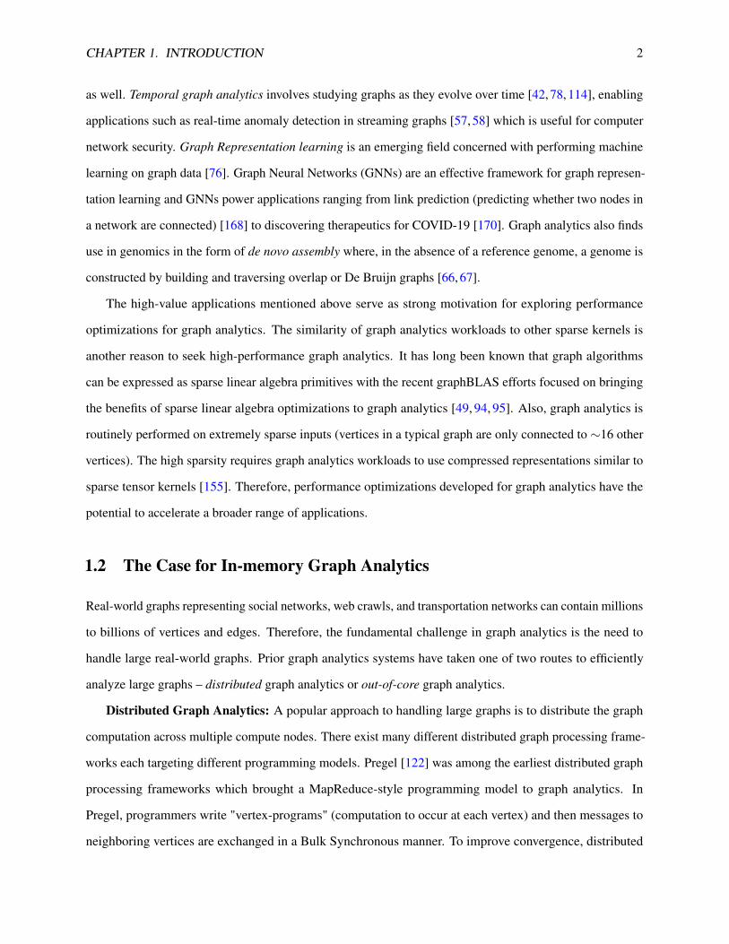
as well. Temporal graph analytics involves studying graphs as they evolve over time [42, 78, 114], enabling
applications such as real-time anomaly detection in streaming graphs [57, 58] which is useful for computer
network security. Graph Representation learning is an emerging field concerned with performing machine
learning on graph data [76]. Graph Neural Networks (GNNs) are an effective framework for graph represen-
tation learning and GNNs power applications ranging from link prediction (predicting whether two nodes in
a network are connected) [168] to discovering therapeutics for COVID-19 [170]. Graph analytics also finds
use in genomics in the form of de novo assembly where, in the absence of a reference genome, a genome is
constructed by building and traversing overlap or De Bruijn graphs [66, 67].
The high-value applications mentioned above serve as strong motivation for exploring performance
optimizations for graph analytics. The similarity of graph analytics workloads to other sparse kernels is
another reason to seek high-performance graph analytics. It has long been known that graph algorithms
can be expressed as sparse linear algebra primitives with the recent graphBLAS efforts focused on bringing
the benefits of sparse linear algebra optimizations to graph analytics [49, 94, 95]. Also, graph analytics is
routinely performed on extremely sparse inputs (vertices in a typical graph are only connected to ∼16 other
vertices). The high sparsity requires graph analytics workloads to use compressed representations similar to
sparse tensor kernels [155]. Therefore, performance optimizations developed for graph analytics have the
potential to accelerate a broader range of applications.
1.2 The Case for In-memory Graph Analytics
Real-world graphs representing social networks, web crawls, and transportation networks can contain millions
to billions of vertices and edges. Therefore, the fundamental challenge in graph analytics is the need to
handle large real-world graphs. Prior graph analytics systems have taken one of two routes to efficiently
analyze large graphs – distributed graph analytics or out-of-core graph analytics.
Distributed Graph Analytics: A popular approach to handling large graphs is to distribute the graph
computation across multiple compute nodes. There exist many different distributed graph processing frame-
works each targeting different programming models. Pregel [122] was among the earliest distributed graph
processing frameworks which brought a MapReduce-style programming model to graph analytics. In
Pregel, programmers write "vertex-programs" (computation to occur at each vertex) and then messages to
neighboring vertices are exchanged in a Bulk Synchronous manner. To improve convergence, distributed

CHAPTER 1. INTRODUCTION 3
frameworks like GraphLab [118] and Vertex Delegates [143] support asynchronous graph execution. Beyond
bulk synchronous and asynchronous execution models, the Powergraph [72] and Powerlyra [40] frameworks
specialize for power-law input graphs 1 which are common in the real-world. While the distributed frame-
works discussed so far target multi-core CPUs, graph computation can also be distributed across multiple
GPUs. Distributed graph processing is critical for GPUs because of the limited memory capacity available
within a single GPU. Frameworks such as Lux [89], multi-GPU Gunrock [141], D-IrGL [87] aim to bring the
throughput advantages of GPUs to larger graphs that do not fit within a single GPU. There has also been
recent effort on developing communication substrates that can transparently distribute shared-memory graph
analytics systems across distributed, heterogeneous (CPUs and GPUs) compute nodes [47, 48].
The primary challenge in distributed graph analytics is to reduce communication between compute nodes.
Instead of randomly dividing the input graph across compute nodes, careful partitioning of the graph is
required for reducing expensive accesses to remote compute nodes [40, 72, 87]. Unfortunately, power-law
input graphs (which are common in the real-world) are hard to partition effectively [109,116]. Prior work has
also shown that the best partitioning strategy can vary with the application, input, and number of compute
nodes [69]. Therefore, while distributed graph analytics allows scaling to large graphs, selecting the right
partitioning strategy is a critical challenge for efficient distributed graph analytics.
Out-of-core Graph Analytics: A second approach to handling large graphs is to rely on dense secondary
storage devices. In out-of-core graph analytics systems, the graph is typically divided into smaller chunks
and stored in secondary storage. During execution, a chunk of the graph is first loaded from disk to memory,
where the graph chunk is processed and then later written back to disk before moving on the next chunk.
GraphChi [105] was the earliest out-of-core graph analytics system, where the authors were able to show that
a single (Mac Mini) PC with SSD is could provide competitive performance to distributed graph processing
on a cluster. X-Stream [149] and Flashgraph [181] are semi-external out-of-core systems where all the
random accesses (to vertex data) are restricted to main memory and all edge data is sequentially accessed
from secondary storage. In contrast, GridGraph [183] and BigSparse [91] are fully-external out-of-core
systems which relax the requirement to store all the vertex data in main memory, enabling analytics on
much larger graphs. Mosaic [121] combined the benefits of fast storage media (NVMe SSDs) and massively
parallel coprocessors (Xeon Phi) to push the boundary of out-of-core graph analytics by processing a trillion
1Power-law input graphs have a few vertices with a disproportionately higher connectivity than the rest of the graph (for eg.celebrity accounts in twitter receive significantly higher following than accounts of most users).

CHAPTER 1. INTRODUCTION 4
edge graph on a single machine. While out-of-core systems are traditionally single-node systems with a
multi-core CPU, prior work has shown that out-of-core graph analytics principles can also be applied to
GPUs [98], allowing a single GPU to handle significantly larger graphs.
The primary challenge in out-of-core graph analytics is to avoid/reduce random accesses to secondary
storage. To avoid the high cost of random I/O, out-of-core systems use custom graph representations [98,105,
183] and perform non-trivial computation patterns [121, 149] to ensure that accesses to secondary storage are
strictly sequential. While enabling a single compute node to handle larger graphs than what can fit within
memory, out-of-core graph analytics can impose significant (pre-)processing overheads.
Increasing main memory capacity of server-class processors is reducing the need to rely on distributed or
out-of-core graph analytics. Modern workstations typically contain main memory in the range of hundreds
of Gigabytes 2, allowing many real-world graphs to be directly processed from main memory. Prior work
has shown that when the input graph fits within the main memory of a single machine, in-memory graph
analytics is more effective than distributed and out-of-core graph analytics [125]. In-memory graph analytics
also offers a simpler programming model; Twitter implemented the first version of the Who-To-Follow
service by processing the entire twitter graph using a single machine to avoid the complexities of building a
distributed graph processing system [73]. The development of many in-memory graph analytics frameworks
in recent years [12,27,145,154,159,160,175,178] is a testament to the ability to analyze large graphs using a
simple programming model. Recently, Dhulipala et. al. [52] showed that the largest publicly-available graph
– the Hyperlink Web graph (with 3.5 billion vertices and 128 billion edges) – can be efficiently processed
on server-class processor with 1TB of main memory, outperforming many prior out-of-core and distributed
graph processing systems on the same graph. Beyond traditional DDR main memories, Gill et. al. [68]
demonstrated the benefits of using dense non-volatile main memory technologies in graph analytics by
characterizing graph processing performance on a single machine with 6TB of Intel Optane DC Persistent
Memory. Using Optane, the authors were able to analyze the same Hyperlink Web graph directly in its native
graph representation (CSR) and outperform distributed graph analytics systems.
In-memory graph analytics is more efficient than distributed and out-of-core graph analytics since it
completely avoids the partitioning and preprocessing overheads of the latter paradigms. Current trends
suggest increasing main memory capacities (particularly, with the adoption of denser, non-volatile memory
technologies) which will allow processing even larger real-world graphs using just a single machine. There-
2Amazon EC2 even offers single machines with 6-24TBs of main memory [1].

CHAPTER 1. INTRODUCTION 5
fore, the rest of this thesis is devoted to identifying the lingering sources of inefficiencies within in-memory
graph analytics and developing optimizations to address the bottlenecks of in-memory graph analytics.
1.3 The Primary Bottleneck of In-memory Graph Analytics: Poor Locality
While more efficient than distributed and out-of-core graph analytics, in-memory graph analytics performance
is still sub-optimal. Graph analytics workloads exhibit very poor cache locality which causes them to be
significantly memory-bound [25, 152, 169] (we characterize the memory-bound nature of graph applications
through roofline analysis in Section 1.4.2). Prior work has shown that, due to poor locality, graph applications
can spend up to 80% of their execution time stalled on DRAM accesses [169]. The primary reason for poor
cache locality of graph analytics workloads is their characteristic irregular memory access pattern. Irregular
memory accesses are fundamental to graph analytics workloads and are the product of using compressed
representations to store the input graphs in a memory-efficient manner. The irregular memory access pattern
coupled with the need to process large inputs causes graph analytics workloads to use the on-chip cache
hierarchy sub-optimally.
PR BC SSSP BFS CC_AF CC_SV TC GMEANGraph Applications
0%
20%
40%
60%
80%
100%
LLC
Hit
Rat
e
Figure 1.1: Locality of graph analytics workloads: Graph applications exhibit a poor LLC hit rate.
We characterized the Last Level Cache (LLC) locality of all the graph applications in the GAP [27]
benchmark suite on a server-class processor (Intel Xeon E5-2660v4) with an LLC capacity of 35MB. Fig-
ure 1.1 reports the LLC hit rate (collected using hardware performance counters [162]) of the different
graph applications running on the Twitter-2010 graph [104]. The result shows that, even with a relatively
large LLC capacity, graph analytics workloads exhibit poor cache locality with only a 40% average LLC
hit rate% 3. While poor cache hit rates may seem intrinsic to the fundamentally pointer-chasing graph3Breadth First Search (BFS) and Connected Components-Afforest algorithm [161] (CC_AF) are exceptions because they exhibit
a high LLC hit rate. BFS uses a bitvector to represent explored vertices which significantly reduces the working set size. CC_AF usesa sampling algorithm to visit only a small portion of the entire graph, boosting its cache hit rate compared to the traditional ShiloachVishkin algorithm (CC_SV).

CHAPTER 1. INTRODUCTION 6
applications, we show that there is significant room for improving the cache locality of graph analytics:
The thesis of this work is that graph analytics workloads have significant structure in their irregular
access patterns, which can be leveraged to improve cache locality. Specifically, the structural properties of
input graphs, common compressed representations, and application access patterns all contain valuable
information that allow optimizing the locality of irregular graph applications.
1.4 Factors Affecting Cache Locality of Graph Analytics
Irregular memory accesses are the primary reason for poor cache locality in graph analytics workloads.
Multiple different factors contribute to irregular memory accesses in graph analytics. To better understand
these different sources of irregularity, this section provides a primer on in-memory graph analytics. We also
quantify the extent to which the different aspects of graph analytics – data structures, applications, and input
graphs – affect cache locality. This knowledge of how different sources of irregular memory accesses affect
graph analytics performance informs the cache locality optimizations we proposed in this thesis.
1.4.1 Graph Data Structures
While there is diversity in the optimizations employed by different graph analytics frameworks [152],
in-memory graph analytics frameworks share similarities in the data structures used to represent graphs,
application access patterns, and the sparsity patterns of typical input graphs. Graph analytics workloads often
analyze extremely sparse inputs (the adjacency matrix representation of typical graphs is >99% sparse [50]).
Therefore, compressed formats are essential for efficiently storing the input graph in memory (Figure 1.2).
The simplest compressed representation – EdgeList or COO (Coordinates format) – stores a list of (source
and destination vertex) coordinates for each edge in the graph. The Compressed Sparse Row (CSR) format
enables a more memory-efficient representation of the graph by sorting the edgelist. As shown in Figure 1.2,
CSR uses two arrays to represent outgoing edges4 (sorted by vertex source IDs). The Neighbors Array (NA)
contiguously stores each vertex’s neighbors and the Offsets Array (OA) stores the starting offset of each
vertex’s neighborhood in the NA. Accessing the ith and (i+ 1)th entries of the OA allows locating vertex
i’s neighbors in the NA. The OA also allows quick estimation of vertex degree: vertex i’s neighbor count is
the difference between the values in the i+ 1 and i entries in the OA. Due to its ability to quickly identify a
4A directed edge connecting vertex i to vertex j, would be considered an outgoing edge of vertex i and an incoming edge ofvertex j.
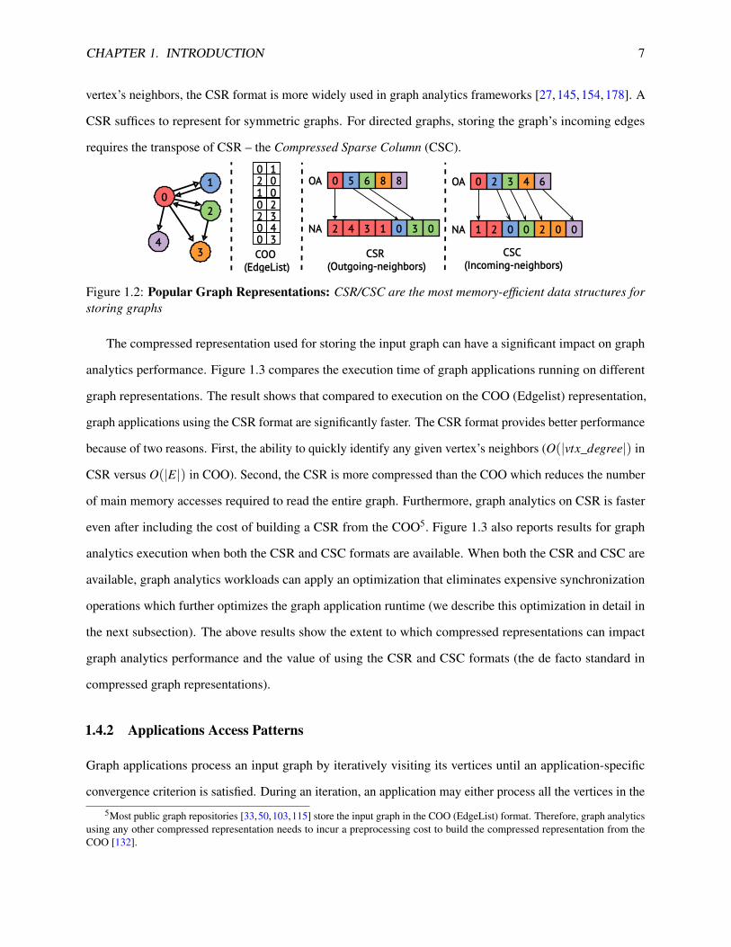
CHAPTER 1. INTRODUCTION 7
vertex’s neighbors, the CSR format is more widely used in graph analytics frameworks [27, 145, 154, 178]. A
CSR suffices to represent for symmetric graphs. For directed graphs, storing the graph’s incoming edges
requires the transpose of CSR – the Compressed Sparse Column (CSC).
01
2
34
0
2 4 3 1
5 6
3
8 8
0 0
OA
NA
0
1 2
2 3
0
4 6
0
OA
NA 2 0 0
COO(EdgeList)
CSC(Incoming-neighbors)
CSR(Outgoing-neighbors)
0 12 01 00 22 30 40 3
Figure 1.2: Popular Graph Representations: CSR/CSC are the most memory-efficient data structures forstoring graphs
The compressed representation used for storing the input graph can have a significant impact on graph
analytics performance. Figure 1.3 compares the execution time of graph applications running on different
graph representations. The result shows that compared to execution on the COO (Edgelist) representation,
graph applications using the CSR format are significantly faster. The CSR format provides better performance
because of two reasons. First, the ability to quickly identify any given vertex’s neighbors (O(|vtx_degree|) in
CSR versus O(|E|) in COO). Second, the CSR is more compressed than the COO which reduces the number
of main memory accesses required to read the entire graph. Furthermore, graph analytics on CSR is faster
even after including the cost of building a CSR from the COO5. Figure 1.3 also reports results for graph
analytics execution when both the CSR and CSC formats are available. When both the CSR and CSC are
available, graph analytics workloads can apply an optimization that eliminates expensive synchronization
operations which further optimizes the graph application runtime (we describe this optimization in detail in
the next subsection). The above results show the extent to which compressed representations can impact
graph analytics performance and the value of using the CSR and CSC formats (the de facto standard in
compressed graph representations).
1.4.2 Applications Access Patterns
Graph applications process an input graph by iteratively visiting its vertices until an application-specific
convergence criterion is satisfied. During an iteration, an application may either process all the vertices in the
5Most public graph repositories [33,50,103,115] store the input graph in the COO (EdgeList) format. Therefore, graph analyticsusing any other compressed representation needs to incur a preprocessing cost to build the compressed representation from theCOO [132].

CHAPTER 1. INTRODUCTION 8
PageRank Radii BFSApplications
0.0
0.2
0.4
0.6
0.8
1.0
Nor
mal
ized
Tim
e
COOCSRCSR+CSC
Figure 1.3: Comparison of different graph representations: Operating on CSR (and CSC) is more efficientthan COO even after accounting for the preprocessing cost of building the CSR/CSC from the COO (shadedportion).
graph or only process a subset of vertices called the frontier. Also, during each iteration, vertices belonging
to the next iteration’s frontiers are identified using application-specific logic. Algorithm 1 shows a typical
graph analytics kernel that traverses an input graph, updating dstData values based on srcData. The kernel
processes the vertices in a frontier in parallel (line 1) and accesses the outgoing neighbors of each vertex in
the frontier (line 2). This pattern of traversing the graph is also known as a push style execution because each
src vertex "pushes" updates to its neighboring dst vertices.
Algorithm 1 A typical graph analytics kernel (Push execution)
1: par_for src in Frontier do2: for dst in out_neigh(src) do . Encoded in the CSR3: atomic_increment(dstData[dst], srcData[src]) . Colliding updates of dstData elements
The push-style graph analytics kernel shown above illustrates the key performance challenges faced by
in-memory graph analytics frameworks. First, accesses to dstData elements suffer from poor cache locality.
The sequence of accesses to the dstData array is determined by the contents of the Neighbors Array (NA
in Figure 1.2) of the CSR. As we noted before, the contents of the NA are arbitrarily ordered (defined by
the structure of the input graph) which causes dstData accesses to have low spatial and temporal locality.
Second, in addition to poor cache locality, graph analytics kernels also suffer from synchronization overheads.
Graph kernels must use expensive atomic instructions to synchronize concurrent updates to elements in the
dstData array (line 3 in Algorithm 1). The update requires synchronization because multiple source vertices
can share the same destination vertex as a neighbor, leading to concurrent updates of shared neighbors.
Prior works [26, 32, 154] have explored eliminating the synchronization overheads of graph analytics
workloads by using a pull style execution (Algorithm 2). In contrast to the push execution shown in
Algorithm 1, a pull execution processes the incoming neighbors of every vertex, essentially updating a dst

CHAPTER 1. INTRODUCTION 9
Algorithm 2 Pull version of Algorithm 1
1: par_for dst in G do2: for src in in_neigh(dst) do . Encoded in the CSC3: if src in Frontier then4: dstData[dst] += srcData[src] . Thread-private updates of dstData elements
vertex by "pulling" values from its src neighbors. A pull execution does not require atomic instructions
because each dstData element is only ever updated by a single thread. However, the elimination of atomics
comes at the expense of analyzing redundant edges. The pull execution accesses all the edges in the graph
(lines 1 and 2 in Algorithm 2), even though only edges belonging to source vertices in the frontier need to be
updated (lines 3 and 4 in Algorithm 2). Therefore, in contrast to a push execution (which only accesses edges
emanating from vertices in the frontier), a pull execution is work-inefficient. As a result, graph analytics
frameworks [27,154,178] employ the push-pull direction switching optimization where, in each iteration, the
application switches between a push or a pull execution depending on the frontier’s density. When the frontier
is dense (i.e. most vertices in the graph belong to the frontier), graph applications perform a pull execution to
trade-off of work-efficiency in favor of avoiding atomic updates. For sparse frontiers, graph applications
perform the standard push execution because only a small fraction of the total edges belong to the frontier,
making concurrent updates to a shared neighbor unlikely. In order to use push-pull direction switching, graph
applications need to be able to dynamically switch between analyzing outgoing and incoming neighbors.
Therefore, graph analytics frameworks employing the push-pull optimization store both the CSR and the
CSC [27,154,178]. Figure 1.3 shows that the push-pull optimization (which uses the CSR and CSC) provides
an mean speedup of 2.5x compared to the standard push execution (which uses only the CSR).
Most graph analytics workloads [27, 154, 178] are essentially variations of the typical kernels shown in
Algorithms 1 and 2 with differences in the update operators used (eg. minimum, logical OR, etc), number of
vertices belonging to the frontier, and the data types of dstData and srcData arrays. To quantify the extent
of performance variation caused by the above application-level factors, we performed Roofline analysis [165]
for a set of graph analytics workloads on a large multi-core processor. Figure 1.4 shows the measured
peak floating point throughput and DRAM bandwidth for our server-class, multi-core processor (Intel Xeon
E5-2660v4) and the measured throughput for a set of graph applications that perform floating point arithmetic.
The different throughput points for each application indicate the executions on different input graphs (we
discuss the variation in performance with respect to inputs in the next subsection). The result shows that
variations in application-level properties (for e.g., frontier density, data types of vertex data, etc.) can cause

CHAPTER 1. INTRODUCTION 10
10 3 10 2 10 1 100 101
Operational Intensity (FLOPs / Bytes)107
108
109
1010
1011
1012
Thro
ughp
ut (
FLO
Ps/s
)
Peak GFLOP/s = 889.33
Peak DRAM BW (GB/s)
= 64.72
PageRankPR-DeltaBetweenness CentralityTriangle CountingSSSP-DeltaStepping
Figure 1.4: Roofline plot for graph analytics workloads: Graph applications are memory-bound and havepoor DRAM bandwidth utilization.
an application to have significantly different operational intensity (the number of floating point operations
performed for every byte read from DRAM). However, despite the differences in operational intensity,
graph analytics workloads are universally bad at saturating DRAM bandwidth (with a mean headroom for
throughput improvement of 5.7x). The above result shows that while there is diversity in the performance
trends of different graph applications, there is still significant opportunity across the board for improving
performance through better bandwidth utilization (by improving cache locality).
1.4.3 Structural Properties of Input Graphs
Real-world input graphs do not have a completely random sparsity pattern. Instead, real-world graphs exhibit
structured sparsity patterns that tend to have a significant impact on performance of graph analytics workloads.
As Figure 1.4 shows, executions of the same graph application on different types of input graphs achieve
vastly different performance. For example, the PR-Delta application achieves throughput ranging from 518
MegaFLOPs to 1.5 GigaFLOPS depending on the sparsity pattern of the input graphs. Performance varies
across inputs because structural properties of the input graphs dictate the amount of reuse for vertex data
elements. Therefore, graph application executions across different input graphs tend to use the on-chip cache
hierarchy with varying levels of effectiveness.

CHAPTER 1. INTRODUCTION 11
Graphs like social networks and web crawls tend to exhibit two structural properties that offer significant
opportunities for data reuse – power-law degree distributions and community structure. Graphs with a power-
law degree distribution [24] contain a small number of vertices (called "hubs") that have a disproportionately
high connectivity, accounting for a majority of the graph’s edges. When analyzing power-law input graphs, a
majority of the vertex data accesses are to the elements corresponding to hub vertices. Graphs with community
structure are composed of islands of densely connected subgraphs (communities) with few connections
between these communities [70]. When analyzing community-structured input graphs, data elements
belonging to vertices in the same community are likely to be accessed in tandem. The power-law degree
distributions and community structures present significant reuse opportunities by controlling/modifying the
assignments of IDs to vertices ("vertex ordering"). Assigning hub vertices in power-law graph consecutive IDs
is likely to boost temporal and spatial locality for the heavily-accessed hub vertices. Similarly, for community-
structured graphs, assigning consecutive IDs to vertices belonging to the same community can improve data
reuse in on-chip caches. We study the impact of changing vertex orders based on the structural property of
the input graph by measuring the cache locality achieved by the Pagerank graph application for different
vertex orders of the PLD input graph (a real-world graph exhibiting both power-law degree distribution and
community-structure [112]). Figure 1.5 compares the Last Level Cache (LLC) misses of different vertex
orders relative to the original ordering of vertices in the PLD graph. The result shows that vertex order
which leverage the power-law degree distribution (for eg, HUBCLUSTER, HUBSORT, DEGSORT) and
community-structure (for eg, RABBIT) can significantly reduce LLC misses and improve cache locality.
However, modifying the vertex order is not a panacea for addressing the poor cache locality problem of graph
analytics because real-world graphs may not always strictly map to a power-law distribution [36] or have
a strong community structure [116]. As a result, the amount of reuse that can be extracted from a graph’s
sparsity pattern will vary.
1.5 Outline of Thesis Contributions
The previous section showed how the different sources of irregularity in graph analytics – structural properties
of input graphs, compressed representations, and application access patterns – affect the cache locality and
performance of graph applications. As mentioned in Section 1.3, the main insight of this thesis is that the
different sources of irregularity in graph analytics also contain information that can be used to improve

CHAPTER 1. INTRODUCTION 12
ORIGINAL RANDOM HUBCLUSTER HUBSORT DEGSORT RABBIT GORDERVertex Orders
0.00.20.40.60.81.01.21.4 Normalized LLC Misses
Figure 1.5: Cache locality from different vertex orders: Changing vertex data layout based on structuralproperties of real-world inputs can increase reuse in on-chip caches.
locality of graph applications. With this insight, we developed four cache locality optimizations for graph
analytics:
Selective Graph Reordering (Chapter 2): We have already seen that changing the ordering of vertices
based on structural properties of input graphs is a critical tool for improving cache locality (Figure 1.5).
However, existing graph reordering optimizations for power-law input graphs provide questionable benefits
once reordering overheads are included; offering performance improvements of up to 76% for some graphs
while also degrading performance by almost 37% for other graphs. To make graph reordering a practical
optimization, we developed an inexpensive analytical model called the Packing Factor which analyzes
the extent to which a graph’s degree distribution matches power-law and uses this information to estimate
performance improvement from graph reordering. The high accuracy of Packing Factor’s speedup prediction
enables selective application of graph reordering, allowing us to preserve the speedups that come from
unconditionally reordering graphs while also restricting the worst-case performance degradation to less than
0.1%. In summary, analyzing the structure of input graphs allows us to predict the extent of benefits from
graph reordering and determine whether reordering the graph would be a worthwhile optimization.
RADAR (Chapter 3): As discussed in Section 1.4.2, graph analytics workloads are bottlenecked not
only by poor cache locality but also by expensive synchronization overheads (due to the need to use atomic
updates). Existing graph analytics optimizations targeted at reducing synchronization overheads do so at the
expense of work-efficiency (i.e. they perform redundant memory accesses to eliminate atomic updates). We
explore a synchronization optimization called RADAR that reduces atomic updates without affecting the
work-efficiency of graph applications. RADAR is a memory-efficient data duplication strategy based on the
observation that, for power-law graphs, a bulk of the atomic updates will only be to the small subset of highly
connected "hub" vertices which allows creating thread-private copies only for the hubs. RADAR builds upon
graph reordering to efficiently identify the hub vertices in a graph and avoid atomic updates for the hubs. In

CHAPTER 1. INTRODUCTION 13
summary, by leveraging the pattern of atomic updates in power-law input graphs, RADAR is able to combine
data duplication with graph reordering to provide superior cache locality and scalability compared to prior
optimizations.
P-OPT (Chapter 4): We have seen that graph applications make sub-optimal use of on-chip caches and
receive very low cache hit rates (Figure 1.1). While decades of research has produced high-performance cache
replacement policies effective at improving locality across various workloads, state-of-the-art replacement
policies are ineffective for graph analytics workloads. Graph application data reuse is complex and the
heuristics used by existing replacement policies are a poor fit for graph applications. Therefore, we set out on
designing a cache replacement policy called P-OPT tailored to the unique access patterns of graph analytics
workloads. P-OPT is based on the observation that most popular graph representation (Section 1.4.1) –
CSR and CSC – efficiently encodes information about future accesses of graph application data. The
easy availability of future access information basically makes Belady’s optimal cache replacement policy
viable for graph analytics workloads. In summary, by leveraging information present within popular graph
representations, P-OPT is able to use the graph’s structure to perform near-optimal cache replacement and
improve cache locality.
HARP (Chapter 5): Irregular memory accesses are the primary contributor to poor cache locality in
graph analytics workloads. Recently, a software-based locality optimization called Propagation Blocking
(PB) was developed for improving cache locality of graph applications performing irregular updates 6. Due to
the pervasiveness of irregular updates, PB turns out to be effective at improving locality for a much broader
range of workloads beyond just graph analytics. However, by virtue of being a software-based optimization,
the locality benefits of PB come at the expense of executing extra instructions and incurring data orchestration
overheads. We developed HARP, a set of architecture extensions aimed to eliminating the bottlenecks of a
PB execution, to improve the performance benefits offered by PB. In summary, by providing architecture
support for a versatile software optimization (PB) that leverages a common application access pattern –
irregular updates – HARP is able to improve performance across a broad range of workloads.
The cache locality optimizations proposed in this thesis include both software-based solutions (Selective
Graph Reordering and RADAR) as well as architectural solutions (P-OPT and HARP). Each optimization
leverages a different aspect of graph analytics, from the structural property of input graphs to compressed
6Throughout this thesis, irregular updates refer to read-modify-write operations on irregular memory locations. Therefore,irregular updates are distinct from irregular reads. For example, the push phase execution (Algorithm 1) performs irregular updatesto dstData whereas the pull execution (Algorithm 2) performs irregular reads of srcData.

CHAPTER 1. INTRODUCTION 14
representations to application access patterns. The scope of each cache locality optimization is also different.
We summarize all the optimizations proposed in this thesis in Table 1.1.
Optimization Leverages Applies toSelective Reordering& RADAR
Structural Property of InputGraphs
Graph Analytics on power-law input graphs
P-OPT CSR & CSC Representation Graph Analytics in general (Input-agnostic)HARP Application Access Pattern Irregular Update Workloads (Including Graph Analytics).
Table 1.1: Cache locality optimizations proposed in this thesis

Chapter 2
Predicting Graph Reordering Speedups
with Packing Factor
The ordering of vertices in a graph has a significant impact on the cache locality of graph analytics workloads
(Figure 1.5). Graph Reordering is a software-based cache locality optimization that leverages the structural
properties of input graphs (such as power-law degree distribution or community structure) to create a new
graph with an ordering of vertices that improves cache locality. Despite the existence of a large number of
reordering techniques with varying levels of sophistication and effectiveness [13, 23, 34, 43, 92, 108, 110, 117,
144, 164, 176], two properties of graph reordering techniques limit their viability as a universally effective
optimization. First, the speedup benefits from graph reordering techniques vary widely across different graph
applications and inputs. Second, graph reordering techniques do not always provide a net speedup when the
cost of reordering the graph is included. To address the overheads of graph reordering, we begin this chapter
by making the case for lightweight graph reordering techniques which aim to provide a net speedup even
after accounting for the overheads of reordering the graph (Section 2.1). Next in Section 2.2, we discuss the
results of our detailed performance characterization of lightweight reordering techniques that allows us to
identify the categories of applications and input graphs that receive the most benefit from lightweight graph
reordering [17]. Using the characterization study, we develop a simple analytical model called the Packing
Factor that allows for a quick estimation of the benefits from graph reordering for any given input graph.
In Section 2.4, we show how the Packing Factor enables selective lightweight graph reordering where the
overheads of graph reordering are only incurred for input graphs that will receive high speedup benefits;
15
CHAPTER 2. PREDICTING GRAPH REORDERING SPEEDUPS WITH PACKING FACTOR 16
improving the viability of lightweight graph reordering. We conclude this chapter by discussing extensions
for the Packing Factor metric to target a variety of graph structures and reordering algorithms (Section 2.6).
2.1 The Case for Lightweight Graph Reordering
Graph reordering techniques improve locality of graph analytics workloads by improving the data layout
of the input based on structural properties of the graph. However, creating a new ordering of vertices and
building a graph reflecting the new vertex order is a preprocessing overhead imposed by graph reordering.
With the exception of a few works [13, 17], most prior studies ignore the preprocessing overheads of graph
reordering. The main assumption used to ignore overheads – that the costs of reordering the graph can be
amortized over multiple executions on the reordered graph – does not hold true in many important application
scenarios. Prior work [42, 78, 136] noted that graph analysis might need to be performed on snapshots of
dynamically evolving graphs at different instants of time (referred to as temporal graph mining). Examples
of such temporal analyses include computing the top webpages (based on their page ranks) in dynamically
changing social networks [104] or tracking changes in the diameter of an evolving graph [114]. In such
application scenarios, an input graph is often processed only once which makes it hard to amortize the
overheads of sophisticated graph reordering techniques [129].
To highlight the overheads of graph reordering, we measure the reordering costs of Gorder, a state-of-the-
art technique that has been shown to outperform various prior reordering algorithms [164]. Gorder uses an
approximation algorithm to solve the NP-hard problem of finding an optimal vertex ordering that maximizes
the overlap between neighborhoods of vertices with consecutive IDs. Table 2.1 shows the run times for the
GAP implementation of the PageRank application on five different graphs with 56 threads (Experimental
setup in Section 2.2.4). “Baseline” runs PageRank on the original graph, “Gorder” runs PageRank after
reordering the graph with Gorder. The Gorder overhead is the time to run the authors’ original Gorder
implementation (which is single-threaded). Gorder consistently improves PageRank’s performance across all
input graphs with a run time reduction on average 35% and with a maximum reduction of 61%.
While Gorder is effective at reducing application run time, the overhead is extremely high. Gorder’s
worst case overhead adds a time cost equal to 1200× the original run time of the PageRank application.
Even if Gorder was perfectly parallelizable (our initial investigations suggest it is not), its run time on our
system would be 21× the run time of PageRank. The table also shows the minimum number of executions of

CHAPTER 2. PREDICTING GRAPH REORDERING SPEEDUPS WITH PACKING FACTOR 17
gplus web pld-arc twitter kron26PageRank Run Time on original graph 6.40s 7.84s 12.40s 21.3s 12.88sPageRank Run Time on Gorder-ed graph 4.48s 7.77s 6.54s 13.09s 5.01sOverhead (Gorder Run Time) 1685.9s 459.8s 7255s 25200s 53234sNumber of runs required to amortize overhead 873 6477 1237 3072 6771
Table 2.1: Reordering overhead of Gorder: Gorder improves performance but with extreme overhead.
PageRank on the reordered graph required to amortize the overhead of Gorder. Across input graphs, a large
number of runs are required to justify the overhead of reordering the graph using Gorder. Gorder might be a
viable reordering technique in scenarios the reordered graph will be processed thousands of times. However,
in other cases where the graph is only expected to be analyzed a couple of times (for example, temporal
graph mining or one-shot execution on a graph), sophisticated reordering techniques such as Gorder are a
de-optimization.
2.2 Performance Improvements from Lightweight Graph Reordering
Results from the previous section (Table 2.1) highlight the need for lightweight reordering techniques that
can improve the performance of graph applications without imposing prohibitively high overheads. In this
section, we show that Lightweight Reordering (LWR) techniques can indeed provide a net speedup even
after including reordering overheads. However, the benefits from LWR are highly dependent on the specific
graph application and input. To identify the categories of graph applications and inputs that benefit the most
from LWR, we characterized performance benefits from three LWR techniques across a diverse set of graph
applications spanning two graph benchmark suites running on large real-world input graphs that stressed the
memory limitations of our evaluation platforms. We provide a brief description of the LWR techniques, graph
applications, input graphs and evaluation platform before presenting the results of our characterization study.
2.2.1 Lightweight Reordering Techniques
We consider three representative Lightweight Reordering (LWR) techniques – Rabbit, HubSort, and Hub-
Cluster.
Rabbit. Rabbit Ordering [13] is a recently proposed lightweight graph reordering technique that exploits
the community structure of graphs. The key idea of Rabbit Ordering is to map the hierarchically dense
communities in graphs to different levels of the cache hierarchy with the most densely connected communities

CHAPTER 2. PREDICTING GRAPH REORDERING SPEEDUPS WITH PACKING FACTOR 18
being mapped to caches closer to the processor. The authors of Rabbit Ordering use a scalable algorithm
for rapid community detection allowing Rabbit Ordering to provide end-to-end performance improvements
compared to other commonly used graph reordering techniques [13].
Hub Sorting. Frequency based clustering [177] (or “hub sorting”) is another lightweight reordering
technique. Hub Sorting relabels the hub vertices 1 in descending order of degrees, while retaining the vertex
ID assignment for most non-hub vertices. Hub Sorting improves spatial and temporal locality of vertex data
accesses for power-law graphs. Spatial locality of vertex data accesses is improved since assigning vertices in
descending order of degree places the most highly accessed elements of vertex data (i.e. hub vertices) in the
same cache line. Temporal locality of vertex data accesses is improved since assigning the highly accessed
hub vertices a contiguous range of IDs increases the likelihood of serving requests to high-reuse portion of
the vertex data from on-chip caches.
Hub Clustering: Hub Clustering is our variation of Hub Sorting that ensures hub vertices are assigned a
contiguous range of IDs, but does not guarantee that the vertex IDs are assigned in descending order of degree.
Hub Clustering improves temporal locality of vertex data accesses by ensuring tight packing of high-reuse
hub vertex data. Hub Clustering incurs lower reordering overhead compared to Hub Sorting since it does not
sort the hub vertices in descending order of degree and consequently provides reduced speedup compared
to Hub Sorting since it misses the opportunity to improve spatial locality by placing the most frequently
accessed vertices in the same cache line. We included Hub Clustering in our evaluation to understand the
trade-off between reordering overhead and the effectiveness of the reordering produced.
For Hub Sorting and Hub Clustering, the vertices are sorted by out-degrees for pull implementations
(or pull-phase dominated implementations) and in-degrees for push implementations. The rationale for the
decision is that vertices with high out-degree will be in-neighbors of many vertices, occurring frequently
in the Neighbor Array (NA) of the graph’s CSC (for example, vertex 0 in Figure 1.2 constitutes majority
of the CSC’s NA). Since accesses to vertex data are determined by the composition of the NA of a graph’s
CSC (srcData accesses in line 4 of Algorithm 2), a pull-based implementation will make a majority of the
accesses to high out-degree vertices because the algorithm iterates over its in-neighbors. Sorting vertices by
out-degrees for pull implementations will, therefore, increase the likelihood of frequently accessed vertices
being cached. Symmetrically, a push-based algorithm is likely to make majority of its accesses to vertices
with high in-degree because the algorithm iterates over its out-neighbors and, hence, would benefit from
1We define hub vertices as vertices with degree greater than average degree.

CHAPTER 2. PREDICTING GRAPH REORDERING SPEEDUPS WITH PACKING FACTOR 19
ordering vertices in descending order of in-degrees.
Figure 2.1 shows vertex ID reassignment produced by Degree Sorting, Hub Sorting, and Hub Clustering.
We omit Gorder and Rabbit Ordering because they are difficult to visualize.
Vertex Degrees (Original)
25 494 4 420 21 6499 6
v0 v1 v2 v3 v4 v5 v6 v7 v8 v9
Vertex Degrees (Degree Sorted)
21 449 464 25 420 6
v0 v1 v2 v3 v4 v5 v6 v7 v8 v9
99
Vertex Degrees (Hub Sorted)
25 499 49 464 21 204 6
v0 v1 v2 v3 v4 v5 v6 v7 v8 v9
Vertex Degrees (Hub Clustered)
25 2099 64 449 21 44 6
v0 v1 v2 v3 v4 v5 v6 v7 v8 v9
Figure 2.1: Vertex ID assignments generated by different reordering techniques: Vertex IDs are shownbelow the degree of the vertex. Highly connected (hub) vertices have been highlighted. Degree Sorting isonly shown for instructive purposes
2.2.2 Graph Applications
We used 11 applications from the GAP [27] and Ligra [154] benchmark suites. All the applications were
compiled using g++-6.3 with -O3 optimization level and OpenMP [46] for parallelization. We evaluated all
applications in the two benchmark suites with the only exception of Triangle Counting. We exclude Triangle
Counting from our evaluation because the GAP implementation already applies a common optimization of
reordering vertices in decreasing order of degree.
We provide a brief description of the execution characteristics of each application and refer the reader to
the original references for additional information [27, 154].
Page Rank (PR-G and PR-L): Page Rank [35] is a popular graph benchmark that iteratively refines per-
vertex ranks until the sum of all ranks drops below a convergence threshold. The implementation performs
pull-style accesses every iteration and processes all the vertices each iteration, causing many random reads to
vertex data (srcData). The GAP and Ligra implementations are similar with the only significant difference
being that Ligra uses a lower default convergence threshold (1e−7 vs 1e−4) leading to a longer application
runtime.
Radii Estimation (Radii-L): Graph Radii estimation approximates the diameter of a graph (longest shortest
path) by simultaneously performing multiple BFS traversals from different random sources. As a consequence
of performing multiple BFS traversals, the application processes a large fraction of the total number of
edges; visiting each vertex multiple times that leads to reuse of vertex data accesses. To avoid the cost of

CHAPTER 2. PREDICTING GRAPH REORDERING SPEEDUPS WITH PACKING FACTOR 20
synchronization, the implementation processes large frontiers using pull-style accesses.
Collaborative Filtering (CF-L): Collaborative filtering is commonly used in recommender systems and
has execution characteristics similar to Page Rank (processing all the vertices each iteration and performing
pull-style accesses every iteration). However, CF has two distinguishing features. First, the application
operates only on weighted symmetric bipartite graphs causing CF to have a unique access pattern to vertex
data (discussed in Section 2.2.5). Second, CF has a significantly larger per-element size of vertex data
compared to other applications (160B versus 4/8B) leading to a significantly larger vertex data working set
size.
Components (Comp-G and Comp-L): Connected components is used to find disconnected subgraphs in a
graph. Components iteratively refines the labels of each vertex until all the vertices in a connected component
share the same label. The algorithm causes the application to process a large fraction of total edges during
the initial iterations of the computation. The main distinction between the GAP and Ligra implementations is
that GAP supports directed graphs while the Ligra implementation only processes undirected (symmetric)
graphs.
Maximal Independent Set (MIS-L): MIS iteratively refines per-vertex labels to find largest independent
set (set of vertices wherein no two vertices are connected) in a graph. The application has execution
characteristics similar to the Ligra implementation of Components. Both applications operate on undirected
graphs and perform pull-style accesses during the initial iterations when the frontier sizes are large.
Page Rank-Delta (PR-Delta-L): Page Rank Delta is a variant of Page Rank that only processes a subset
of vertices for which the rank value changed beyond a δ amount. While Page Rank Delta does not process
all the vertices every iteration like Page Rank, the application processes large frontiers during the initial
iterations of the computation. In contrast to most other Ligra applications, the implementation does not
switch between push and pull style accesses based on frontier sizes and performs push-style accesses every
iteration.
SSSP-Bellman Ford (SSSP-L): The Ligra implementation of SSSP uses the Bellman Ford algorithm. Due
to the work inefficient nature of the Bellman Ford algorithm, the application processes a significant fraction
of total edges in the initial iterations and, hence, offer reuse in vertex data accesses. Similar to Page Rank
Delta, the SSSP implementation does not switch between push and pull style accesses and always performs
push-style accesses.
Betweenness Centrality (BC-G and BC-L): Betweenness Centrality finds the most central vertices in a

CHAPTER 2. PREDICTING GRAPH REORDERING SPEEDUPS WITH PACKING FACTOR 21
graph by using a BFS kernel to count the number of shortest paths passing through each vertex from a source.
Since the application traverses over a BFS tree of a graph, the application processes a limited fraction of total
edges for most iterations.
SSSP-Delta Stepping (SSSP-G): The GAP implementation of Single Source Shortest Path problem uses
the delta stepping algorithm [127] which strikes a balance between work-efficiency and parallelism. The cost
of updating thread-local containers used for work-efficient scheduling of vertices reduces the fraction of the
application runtime spent executing the irregular access kernel (Algorithm 2). The implementation performs
push-style accesses to process vertices each iteration.
Breadth First Search (BFS-G and BFS-L): The GAP and Ligra implementations of BFS use the push-
pull direction-switching optimization proposed in prior work [26] to reduce the total number of edges
processed relative to a traditional implementation. Consequently, BFS processes the fewest edges among all
applications; offering limited room for performance improvement from locality optimization. Additionally,
the short runtime of the BFS application offers limited room for amortizing the overhead of graph reordering.
K-core Decomposition (KCore-L): KCore is an application that finds sets of vertices (called cores) with
degree greater than K for different values of K. The application takes many iterations (≈1000) to converge
and, hence, has a long runtime. Additionally, the algorithm used for K-core computation causes the executions
to spend only a small fraction (≈10%) of the total run time performing irregular accesses (Algorithm 2).
2.2.3 Input graphs
We use large, real-world input graphs with power-law degree distribution that have been collected from a
variety of datasets for evaluating the performance benefits from lightweight reordering. Table 2.2 lists the
number of vertices, edges, the size of the vertex data array (assuming 8B element size), and the size of a
CSR representation for the graph that are used for majority of our evaluation. We use the graph converters
available in the GAP and Ligra benchmarks to create undirected and/or weighted versions of these graphs
based on the application requirements. For Collaborative Filtering, we use the 8 largest bipartite graphs
available in the Konect dataset [103].

CHAPTER 2. PREDICTING GRAPH REORDERING SPEEDUPS WITH PACKING FACTOR 22
DBP GPL PLD KRON TWIT MPI WEB SD1Reference [103] [71] [126] [29] [104] [103] [51] [126]|V | (in M) 18.27 28.94 42.89 33.55 61.58 52.58 50.64 94.95|E| (in B) 0.172 0.462 0.623 1.047 1.468 1.963 1.93 1.937irregData Sz (MB) 146.16 231.52 343.12 268.4 498.64 420.64 405.12 759.6CSR Sz (GB) 1.41 3.66 4.96 8.05 11.34 15.02 14.75 15.13
Table 2.2: Statistics for the evaluated input graphs: The size of vertex data for all the graphs exceeds theLLC capacity.
2.2.4 Evaluation Platform and Methodology
We performed all our experiments on a dual-socket server machine with two Intel Xeon E5-2660v4 processors.
Each processor has 14 cores, with two hardware threads each, amounting to a total of 56 hardware execution
contexts. Each processor has a 35MB Last Level Cache (LLC) and the server has 64GB of DRAM
provided by eight DIMMs. All experiments were run using 56 threads and we pinned the software thread to
hardware threads to avoid performance variations due to OS thread scheduling. To further reduce sources of
performance variation, we also disabled the “turbo boost” DVFS features and ran all cores at the nominal
frequency of 2GHz.
We ran 17 trials for each application-input pair and report the geometric mean of the 16 trials. We exclude
the timing of the first trial to allow the caches to warm up. For source-dependent traversal applications (e.g.
BFS, SSSP, BC, etc.), we select a source vertex belonging to the largest connected component to ensure that a
significant fraction of the graph is traversed. To identify such a source, we ran 100 trials of these applications
with different sources and selected the source that traversed the maximum number of edges in the graph.
We also maintain a mapping between the vertex ID assignments before and after reordering to ensure that
traversal applications running on the reordered graphs use the same source as the baseline execution running
on the original graph [29].
2.2.5 Characterization Study Results
Lightweight reordering (LWR) techniques improve graph processing performance with low overhead. How-
ever, speedup from LWR depends on the LWR technique used, application characteristics, and properties of
the input graph. This subsection identifies the characteristics of applications that receive end-to-end perfor-
mance benefits from LWR, by studying three techniques (of varied sophistication and overhead) – Rabbit
Ordering, Hub Sorting, and Hub Clustering – across the applications and graphs presented in Sections 2.2.2

CHAPTER 2. PREDICTING GRAPH REORDERING SPEEDUPS WITH PACKING FACTOR 23
DBP GPL PLD KRON TWIT MPI WEB SD10.00.51.01.52.0
Spee
dup
PR-L
DBP GPL PLD KRON TWIT MPI WEB SD10.00.51.01.52.0 2.7x2.7x2.7x2.7x2.7x2.7x2.7x2.7x2.7x2.7x2.7x2.7x2.7x2.7x2.7x
PR-G
DBP GPL PLD KRON TWIT MPI WEB SD10.00.51.01.52.0
Radii-L
DBLP DISC WIKI EDIT LIVEJ ORK DELI TRACK0.00.51.01.52.0
Spee
dup
CF-L
DBP GPL PLD KRON TWIT MPI WEB SD10.00.51.01.52.0 3.5x 2.6x3.5x 2.6x3.5x 2.6x3.5x 2.6x3.5x 2.6x3.5x 2.6x3.5x 2.6x3.5x 2.6x3.5x 2.6x3.5x 2.6x3.5x 2.6x3.5x 2.6x3.5x 2.6x3.5x 2.6x3.5x 2.6x
COMP-G
DBP GPL PLD KRON TWIT0.00.51.01.52.0
COMP-L
DBP GPL PLD KRON TWIT0.00.51.01.52.02.53.0
Spee
dup
11.7x 8.4x11.7x 8.4x11.7x 8.4x11.7x 8.4x11.7x 8.4x11.7x 8.4x11.7x 8.4x11.7x 8.4x11.7x 8.4x11.7x 8.4x11.7x 8.4x11.7x 8.4x11.7x 8.4x11.7x 8.4x11.7x 8.4x MIS-L
DBP GPL PLD KRON TWIT MPI WEB SD10.00.51.01.52.0
PR-Delta-L
DBP GPL PLD KRON TWIT MPI WEB SD10.00.51.01.52.0
SSSP-L
DBP GPL PLD KRON TWIT MPI WEB SD10.00.51.01.52.0
Spee
dup
BC-L
DBP GPL PLD KRON TWIT MPI WEB SD10.00.51.01.52.0
BC-G
DBP GPL PLD KRON TWIT MPI WEB SD10.00.51.01.52.0
SSSP-G
DBP GPL PLD KRON TWIT MPI WEB SD1Input Graphs
0.000.250.500.751.001.25
Spee
dup
BFS-L
DBP GPL PLD KRON TWIT MPI WEB SD1Input Graphs
0.000.250.500.751.001.25 BFS-G
DBP GPL PLD KRON TWITInput Graphs
0.000.250.500.751.001.25 KCore-L
RabbitHubSortHubCluster
Figure 2.2: Speedup after lightweight reordering: Data are normalized to run time with the original vertexordering. The total bar height is speedup without accounting for the overhead of lightweight reordering.The upper, hashed part of the bar represents the overhead imposed by lightweight reordering. The filled,lower bar segment is the net performance improvement accounting for overhead. The benchmark suites aredifferentiated using a suffix (G/L).
and 2.2.3.
Figure 2.2 plots LWR performance improvements for each application and several input graphs. For each
execution (application + input graph + LWR technique), we show speedup without reordering overhead (total
bar height) and end-to-end speedup accounting for the overheads (solid bar). The baseline is an execution on
the input graph as originally ordered by the publishers of the graph datasets [51, 103, 115, 126]. We do not
have data for Rabbit Ordering on MPI, WEB, and SD1 because Rabbit Ordering exhausts our machine’s
64GB of memory for these graphs. We also omit data for COMP-L, MIS-L, and KCore-L for the undirected
versions of the same graphs because the applications run out of memory.
To understand variation in performance across applications, we measured the average fraction of edges
processed in an iteration across applications from Ligra (shown in Table 2.3). We weight the fraction of edges
processed in an iteration by the fraction of total execution time spent in that iteration to focus on iterations
that dominate runtime. The data in Table 2.3 help explain the benefit due to LWR, which we present next.
Finding 1: Lightweight reordering can provide end-to-end speedups. Figure 2.2 shows that the Page
Rank (GAP and Ligra), Radii, Collaborative Filtering, Components, and MIS see a net speedup including

CHAPTER 2. PREDICTING GRAPH REORDERING SPEEDUPS WITH PACKING FACTOR 24
DBP GPL PLD KRON TWIT MPI WEB SD1 AVGPR 100 100 100 100 100 100 100 100 100Radii 55.59 71.79 69.82 87.97 75.07 72.35 41.39 43.19 64.65CF 100 100 100 100 100 100 100 100 100BFS 1.31 1.62 1.78 0.74 0.78 0.9 0.22 0.56 0.99BC 22.38 22.63 28.56 43.60 28.98 25.72 9.78 15.72 24.67SSSP 47.72 70.1 59.1 82.31 76.27 67.28 31.97 58.68 61.67PR-δ 80.19 84.45 76.32 90.70 83.31 83.76 76.97 72.36 81.00KCore 0.17 0.03 0.05 1.02 0.02 - - - 0.25COMP 98.69 98.36 83.22 84.03 98.12 - - - 92.48MIS 71.48 56.54 76.68 79.24 54.32 - - - 67.65
Table 2.3: Average percentage of edges processed by Ligra applications: A higher average percentage ofedges processed corresponds to greater reuse in vertex data accesses. The AVG field for each applicationrepresents the average value of the metric across 8 input graphs.
LWR overheads in some cases. Table 2.3 shows that these applications all process a significant fraction of
edges in each iteration. The high average percentage of edges processed leads to significant reuse in vertex
data accesses and offers a higher room for locality improvement from LWR.
Finding 2: Hub Sorting is a good balance of effectiveness and reordering overhead. The data for
Page Rank and Radii reveal a tension between LWR effectiveness and the overhead of graph reordering.
Compared to Hub Clustering, Hub Sorting yields higher speedup (excluding overhead) than Hub Sorting
for the PLD, TWIT, KRON, and SD1 graphs. The higher speedup is due to reordering frequently accessed
vertices in decreasing degree order, improving locality by placing the most frequently accessed vertex data
elements in the same cache line. Hub Clustering misses this opportunity for spatial locality because it does
not store vertices in decreasing degree order. In contrast, Hub Sorting incurs a higher overhead than Hub
Clustering (i.e., the shaded portion in each bar) reducing the difference in the net speedup between the two
techniques, especially for the applications with short runtimes (Radii and GAP’s Page Rank).
The data for Rabbit Ordering reveal a surprising trend: the less sophisticated Hub Sorting algorithm has
higher speedup than the more sophisticated Rabbit Ordering algorithm. Ignoring overhead, Rabbit Ordering
does not consistently outperform Hub Sorting because the authors of Rabbit Ordering use heuristics to
parallelize the reordering algorithm [13]. After accounting for reordering overhead, Hub Sorting consistently
outperforms Rabbit Ordering. The data suggest that for Page Rank and Radii, Hub Sorting is an effective
middle ground, improving performance with low overhead.
Finding 3: Hub Sorting is a poor fit for symmetric bipartite graphs. Figure 2.2 shows that Collabo-
rative Filtering has different performance characteristics than Page Rank despite having similar execution

CHAPTER 2. PREDICTING GRAPH REORDERING SPEEDUPS WITH PACKING FACTOR 25
characteristics. While Rabbit Ordering consistently improves performance, Hub Clustering has the best net
speedup after accounting for overhead. Surprisingly, Hub Sorting causes slowdown for the EDIT, LIVEJ, and
TRACK graphs, even after ignoring reordering overhead.
Collaborative Filtering is different because its input graphs are symmetric and bipartite (i.e., vertices fall
into two parts A or B and no pair of nodes in the same part are connected). Neighbors of a vertex u ∈ A are
in part B and vice versa. Contiguously ordering vertices in a part offers temporal locality because irregular
vertex data accesses are restricted to one part at a time. The base ordering of our bipartite graphs had their
parts originally laid out contiguously. Naively Hub Sorting mixes vertices from different parts, leading to the
slowdown.Base Ordering
Hub Sorting
Hub Clustering
(a) LIVEJ
Base Ordering
Hub Sorting
Hub Clustering
(b) DBLP
Figure 2.3: Vertex orders of a symmetric bipartite graph by Hub Sorting and Hub Clustering: The twocolors represent the parts of the bipartite graph. Hub Sorting produces a vertex order wherein vertices fromdifferent parts are assigned consecutive vertex IDs whereas Hub Clustering produces an ordering wherevertices belonging to the same part are often assigned consecutive IDs.
We studied the part-wise ordering effect by visualizing the part number (A or B) for each vertex in
the base ordering and in the ordering produced by Hub Sorting and Hub Clustering (Figure 2.3) for two
symmetric bipartite graphs. The data show that Hub Clustering is better at preserving part-wise locality
compared to Hub Sorting and, hence, provides better performance.
Finding 4: LWR can affect convergence rate. For Components (GAP and Ligra) and MIS, performance
with LWR varies due to a change in the number of iterations to convergence. Convergence varies because in
these algorithms the total amount of work performed per iteration depends on the vertex ID assignment. Note
that reordering does not affect correctness of these applications. Table 2.4 shows the increase in iterations to
convergence for each LWR technique. Speedups in Figure 2.2 track the variation in iterations to convergence
in most cases. However, the increase in iterations to convergence does not vary consistently with application,
input graph, or LWR technique used.
Finding 5: Push-mode applications benefit less from LWR. SSSP-Bellman Ford (Ligra) and Page Rank

CHAPTER 2. PREDICTING GRAPH REORDERING SPEEDUPS WITH PACKING FACTOR 26
DBP GPL PLD KRON TWIT
Comp-GRabbit 2.39x 2.0x 5.23x 1.33x 1.47xHubSort 1.36x 1.0x 2.09x 0.67x 0.9xHubCluster 1.81x 1.0x 1.05x 0.67x 0.88x
Comp-LRabbit 1.5x 1.25x 1.27x 1.0x 0.99xHubSort 1.25x 1.0x 1.0x 0.67x 0.93xHubCluster 1.25x 1.0x 1.0x 0.83x 0.94x
MIS-LRabbit 0.3x 0.56x 0.56x 0.96x 0.52xHubSort 0.69x 0.56x 0.79x 2.27x 1.01xHubCluster 0.85x 0.85x 0.98x 1.19x 1.02x
Table 2.4: Impact of LWR on iterations until convergence: Values greater than 1 indicate delayedconvergence compared to baseline execution on the original graph. Values less than 1 indicate that theexecution on the reordered graphs converged in fewer iterations than the execution on the original graph.
Delta applications do not speed up with LWR despite processing a large fraction of edges per iteration
(Table 2.3). The distinguishing feature of these two Ligra applications is that they do not use the push-
pull direction optimization, instead using push-mode accesses only. While laying out the most frequently
accessed vertices together improves performance for push-mode applications, doing so may also increases
the likelihood of false sharing, which degrades performance. False sharing affects Page Rank Delta on the
DBP, GPL, and MPI graphs. Consequently, Rabbit Ordering and Hub Sorting cause slowdowns even without
the reordering overhead. SSSP-Bellman Ford has better performance than Page Rank Delta because it is
optimized to use Test&Test&Set [150] operations, which reduces false sharing.
To help understand the loss due to false sharing from LWR in these push-style applications, we evaluated
speedup from LWR after modifying the applications to use the push-pull optimization. Table 2.5 shows
speedups (without overhead) from LWR for these push-pull versions of Page Rank Delta and SSSP-Bellman
Ford. The results shows that all three LWR techniques provide greater speedup when the two applications use
the push-pull optimization compared to when the applications perform push-style accesses throughout the
execution (Figure 2.2). Although the push-pull implementations of Page Rank Delta and SSSP-Bellman Ford
are slower than the push-style implementations, the results of Table 2.5 illustrate that push-style accesses
reduce the performance benefits of LWR, even in applications that process a large fraction of edges per
iteration (Table 2.3).
Finding 6: Applications that process few edges per iteration do not benefit from LWR. Applications
that process a small fraction of edges per iteration (BC, BFS, and KCore) see little benefit from LWR, even
after ignoring reordering overhead. Figure 2.2 shows that these applications consistently see no speedup
from LWR even without accounting for the reordering overhead. The KRON graph is a notable exception,

CHAPTER 2. PREDICTING GRAPH REORDERING SPEEDUPS WITH PACKING FACTOR 27
DBP GPL PLD KRON TWIT
PR-δ -LRabbit 1.11x 1.53x 1.53x 0.92x 1.26xHubSort 0.94x 0.99x 1.43x 1.77x 1.77xHubCluster 1.06x 1.01x 1.24x 1.46x 1.27x
SSSP-LRabbit 0.87x 1.36x 1.2x 0.95x 0.97xHubSort 1.02x 1.14x 1.58x 2.0x 1.4xHubCluster 1.14x 1.07x 1.47x 1.58x 1.4x
Table 2.5: Speedups from LWR for push-pull implementations: LWR techniques provide greater perfor-mance improvements for applications that perform pull-style accesses while processing large frontiers.
seeing appreciable benefit due to its flat graph structure2 offering reuse of vertex data accesses. However, the
real-world graphs in our dataset do not share KRON’s flat structure and, hence, do not benefit from LWR.
The data for BFS and KCore further highlight the lack of benefit with few edges processed per iteration.
Table 2.3 shows that the BFS and KCore application process the fewest edges per iteration of all the
applications we evaluated. The small fraction of edges processed per iteration leads to limited reuse in vertex
data access and offers little room for improvement from LWR.
2.3 When is Lightweight Reordering a Suitable Optimization?
We summarize Section 2.2.5’s analysis across LWR techniques, applications, and input graphs by listing
recommendations for the lightweight reordering technique suitable for different categories of applications.
Takeaway 1: Applications like Page Rank and Radii that process a large fraction of edges in each
iteration in the pull-mode are most amenable to lightweight reordering techniques.
Takeaway 2: Existing lightweight reordering techniques are inappropriate for symmetric bipartite graphs
(as in CF) unless modified to store vertices in each part contiguously in memory.
Takeaway 3: In some cases (e.g., Components and MIS) lightweight reordering changes the number of
iterations to convergence, revealing an opportunity for future techniques leveraging vertex ordering to speed
convergence.
Takeaway 4: Applications that are push-style (e.g., Page Rank Delta and SSSP-Bellman Ford) or process
a few edges per iteration (e.g., BC, SSSP-Delta Stepping, BFS, and KCore) do not benefit from lightweight
reordering because of false-sharing and limited reuse in vertex data accesses respectively. The ineffectiveness
of lightweight reordering in these applications is not due to the overhead of reordering.
2Flat means the BFS tree of KRON is shallow, with a majority of vertices in a few levels of the tree

CHAPTER 2. PREDICTING GRAPH REORDERING SPEEDUPS WITH PACKING FACTOR 28
Takeaway 5: When Hub Sorting is effective (e.g., Page Rank and Radii), its benefit is input graph-
dependent (Figure 2.2), sometimes providing no speedup (e.g., DBP, GPL, MPI, WEB) and instead causing a
net slowdown due to its overhead. The next section studies the characteristics of graphs for which lightweight
reordering provides end-to-end speedups.
2.4 Selective Lightweight Graph Reordering Using the Packing Factor
Hub Sorting is an effective lightweight reordering technique that provide end-to-end performance improve-
ment for applications like Page Rank and Radii. However, the speedup from lightweight reordering depends
on the input graph. Therefore, we cannot unconditionally reorder input graphs because reordering can
sometimes cause slowdowns. This section shows that the graph structure and the original graph ordering
determine the speedup of reordering. We propose a low-overhead metric, called the Packing Factor, to
identify the properties of the input graph critical for achieving speedup from reordering and show that the
Packing Factor metric enables selective application of Hub Sorting.
2.4.1 Input-dependent Speedup from Hub Sorting
The variation in a graph’s structure and its original vertex ID assignment explains the difference in speedups
from Hub Sorting across input graphs. Assigning hub vertices a contiguous range of IDs ensures that the
frequently accessed elements of vertex data (i.e., corresponding to hubs) are packed closely, spanning a small
number of cache lines. The hub vertices in a graph are connected to a significant fraction of the graph with the
hub vertices accounting for 80% of total edges across the graphs shown in Table 2.2. Consequently, accesses
to cache lines containing hubs’ elements in the vertex data are frequent and lines containing tightly-packed
hubs are likely to be frequently reused. These tightly-packed hubs’ cache lines are also likely to remain
resident in the Last Level Cache (LLC), improving locality. Moreover, sorting vertices by decreasing vertex
degree puts the most frequently accessed vertices in the same cache line improving spatial locality.
In order to benefit from Hub Sorting, an input graph must be skewed and its hubs must not already be
tightly-packed before reordering. In a skewed input graph, a few vertices have a disproportionately higher
degree than all other vertices. Skewed graphs allow Hub Sorting to pack the few hubs into even fewer cache
lines, increasing the likelihood that vertex data accesses will hit in the LLC because the hubs’ cache lines
will remain cached. Additionally, to benefit from Hub Sorting, the original layout of hub vertices must also

CHAPTER 2. PREDICTING GRAPH REORDERING SPEEDUPS WITH PACKING FACTOR 29
be sufficiently sparse in memory such that multiple hubs are unlikely to reside in the same cache line. If hub
vertices are originally tightly-packed, Hub Sorting is ineffective because accesses to the hubs will already
have good locality. In contrast, graphs that originally have sparsely distributed hub vertices suffer from poor
temporal and spatial locality. For such graphs, Hub Sorting provides performance gains by reordering the
hub vertices such that the highly accessed vertex data elements span fewer cache lines.
2.4.2 Packing Factor
To identify whether an input graph will benefit from Hub Sorting, we develop Packing Factor, a metric that
quantifies graph skew and the sparsity of hub vertices3. Packing Factor directly computes the decrease in
sparsity of hubs after Hub Sorting. To compute Packing Factor, we compute the original graph’s hub working
set, which is the number of distinct cache lines containing hub vertices. Packing Factor is the ratio of the
original graph’s hub working set to the minimum number of cache lines in which the graph’s hubs can fit,
based solely on cache line capacity. If the original graph’s hub working set is much larger than the minimum
number of lines required for the hub vertices then Packing Factor is high and Hub Sorting is likely to provide
a large benefit by tightly packing the hubs. Algorithm 3 shows the steps involved in computing the hub
working set of the original graph (Lines 4-11) and after performing Hub Sorting (Line 12)
Algorithm 3 Computing the Packing Factor of a graph
1: procedure COMPUTEPACKINGFACTOR(G)2: numHubs← 03: numHubCacheLinesOriginal ← 04: for CacheLine in vDataLines do5: containsHub← False6: for vtx in CacheLine do7: if ISHUB(vtx) then8: numHubs += 19: containsHub← True
10: if containsHub = True then11: numHubCacheLinesOriginal += 1
12: numHubCacheLinesSorted ← CEIL(numHubs/VtxPerLine)13: PackingFactor← numHubCacheLinesOriginal/numHubCacheLinesSorted14: return PackingFactor
To understand the relationship between speedup from Hub Sorting and Packing Factor, we measured
speedup of Page Rank (GAP and Ligra) and Radii on the 8 input graphs from the main evaluation (Figure 2.2)
3We have open-sourced the code for Packing Factor computation and other reordering techniques athttps://github.com/CMUAbstract/Graph-Reordering-IISWC18

CHAPTER 2. PREDICTING GRAPH REORDERING SPEEDUPS WITH PACKING FACTOR 30
and 7 additional input graphs from Konect [103]. Figure 2.4 shows the Hub Sorting speedup (excluding
reordering overhead) and Packing Factor of the input graph for the three applications on 15 graphs. The data
shows a strong correlation (r = 0.9) between speedup from Hub Sorting and Packing Factor of a graph.
1 2 3 4 5 6Packing Factor
1.0
1.5
2.0
2.5
Spee
dup
PR-GPR-LRadii-L
Figure 2.4: Relation between speedup from Hub Sorting and packing factor of input graph: Each pointis a speedup of an application executing on Hub Sorted graph compared to the original graph. Differentapplications are indicated with different colors/markers. Hub Sorting provides significant speedup forexecutions on graphs with high Packing Factor.
The data in Figure 2.4 show that a graph’s Packing Factor is a useful predictor of Hub Sorting’s speedup.
We empirically observe that graphs with a Packing Factor less than 4 do not experience a significant speedup
from Hub Sorting (maximum speedup of 1.25x). For such graphs, speedup is likely to be negated by the
overhead of Hub Sorting, leading to a net slowdown. Based on these data, we conclude that a system should
selectively perform Hub Sorting on graphs with packing factor greater than the threshold value of 4 only.
Selective Hub Sorting yields speedup for graphs with high Packing Factor and avoids degrading performance
for other graphs. We evaluate such a system in Section 2.4.4.

CHAPTER 2. PREDICTING GRAPH REORDERING SPEEDUPS WITH PACKING FACTOR 31
2.4.3 Characterization of Speedup from Hub Sorting
We have seen that Hub Sorting provides significant speedups for certain input graphs and Packing Factor is
an effective metric to identify these graphs. To better understand why Hub Sorting improves performance, we
used native hardware performance counters [162] to analyze executions on reordered graphs. We measured
the reduction in Last Level Cache (LLC) misses and the reduction in Data TLB load misses leading to a page
walk. For these tests, we disabled hyperthreading and ran with only one thread per core (i.e., 28 threads) due
to limitations of the performance counter infrastructure [2]. Figure 2.5 shows the reduction in LLC misses
and DTLB load misses compared to Packing Factor of input graphs for the two applications from Ligra. The
data show that graphs with high Packing Factor get significant reduction in LLC misses and DTLB load
misses from Hub Sorting. The linear relation between LLC and DTLB load miss reduction and Packing
Factor is characteristic of the linear relation between speedup and Packing Factor in Figure 2.4. The data
suggest that the speedup from lightweight reordering are due to reduction in LLC misses (fewer slow DRAM
accesses) and a reduction in DTLB misses (fewer expensive page table walks).
2 4 6Packing Factor
0.5
1.0
1.5
2.0
2.5
3.0
3.5
Red.
in L
LC M
isses
2 4 6Packing Factor
0.0
0.5
1.0
1.5
2.0
2.5
3.0
Red.
in D
TLB
Miss
es
PR-LRadii-L
Figure 2.5: Reduction in LLC and DTLB misses due to Hub Sorting: Hub Sorting provides greaterreduction in LLC misses and DTLB load misses for graphs with high Packing Factor.
2.4.4 Selective Hub Sorting
A graph’s Packing Factor predicts whether Hub Sorting will yield a net speedup. Computing Packing
Factor (Algorithm 3) imposes a low-overhead since it involves a highly-parallelizable scan of vertex degrees.

CHAPTER 2. PREDICTING GRAPH REORDERING SPEEDUPS WITH PACKING FACTOR 32
Figure 2.6 shows the net speedup (including Hub Sorting overhead) for a system that unconditionally reorders
a graph compared to a system that only selectively reorders a graph if the Packing Factor of the graph is
a higher than our empirical threshold of 4. Selective reordering preserves the end-to-end speedup from
unconditional reordering for graphs with high Packing Factor while avoiding slowdowns for graphs with low
Packing Factor. Computing Packing Factor imposes negligible overhead 4, making selective reordering a
practical alternative to unconditional Hub Sorting.
0.000.250.500.751.001.251.50
Spee
dup
PR-G
0.000.250.500.751.001.251.501.75
Spee
dup
PR-L
WEB WIK-EN WIK-DE SPKC SLVJ ORK DBP GPL MPI KAI SD1 PLD TWIT KR25 KR26Input Graphs
0.000.250.500.751.001.25
Spee
dup
Radii-L
AlwaysSelective
Figure 2.6: End-to-end speedup from selective Hub Sorting: Input graphs have been arranged in in-creasing order of Packing Factor. Selective application of Hub Sorting based on Packing Factor providessignificant speedups on graphs with high Packing Factor while avoiding slowdowns on graphs with lowPacking Factor.
2.5 Related Work
Prior research related to this work spans five categories - graph reordering, cache blocking, vertex scheduling,
and graph partitioning.
Graph Reordering: There has been extensive research in developing graph reordering techniques of varying
levels of effectiveness and sophistication. Sophisticated graph reordering techniques such as Gorder [164],
ReCALL [108], Layered Label Propagation (LLP) [34], Nested Dissection [110], SlashBurn [117] provide
significant speedups to the application but incur extremely high overheads. The high overhead of these
techniques are justified only in the cases where the same input graph is expected to be processed multiple
times. In contrast to such high-overhead reordering techniques, recent graph reordering proposals have4Across input graphs, computing the Packing Factor comprised at most 0.1% of the runtime on the original graph

CHAPTER 2. PREDICTING GRAPH REORDERING SPEEDUPS WITH PACKING FACTOR 33
focused on keeping the overhead of reordering low. Karantis et. al. [92] proposed a parallel implementations
of common graph reordering techniques – Reverse Cuthill-McKee (RCM) and Sloan – to reduce reordering
overheads. While parallelization improved the performance of reordering by more than 5x, the authors
report an end-to-end speedup of 1.5x when performing 100 Sparse Matrix Vector (SpMV) iterations. Rabbit
Ordering [13], which was studied in this work, was shown to provide better end-to-end performance
improvements compared to parallel RCM. These research efforts support the need for effective lightweight
reordering techniques to support application use cases where the assumption of amortizing high reordering
overhead across multiple trials is not guaranteed.
Cache blocking: Cache blocking is an alternate technique to improve locality of graph processing appli-
cations. Zhang et. al. [176] recently proposed CSR segmenting – a technique to improve temporal locality
of vertex data accesses by breaking the original graph into subgraphs that reduce the irregularity of vertex
data accesses. The computation from each subgraph are buffered and later merged to produce the final
result. Similar approaches were used in prior work aiming to exploit reuse at the LLC [75, 160]. Recent
proposals [28,37] have extended the idea of partitioning the graph and applied it to partitioning data transfers
between vertices in Sparse Matrix multiplying Dense Vector (SpMV) application such as Page Rank. While
blocking based techniques are effective in improving application performance, they require modifying the
application unlike graph reordering techniques.
Vertex scheduling: Graph reordering techniques improves locality by optimizing the layout of graph data
structures. The locality of graph applications can also be improved by changing the order of processing
vertices. Prior work [125, 134, 177] have shown that traversing the edges of a graph along a Hilbert curve
can create locality in the both the source vertex read from and the destination vertex written to. However,
a key challenge with these techniques is that they can complicate parallelization [28, 176]. HATS [128]
is a dynamic vertex-scheduling architecture that improves cache locality of vertex data accesses. HATS
runs hardware Bounded Depth First Search (BDFS) to schedule vertices, yielding locality improvements
in community-structured graphs. Graph reordering is primarily a data layout optimization and, hence, is
complementary to vertex scheduling.
Graph Partitioning: Graph partitioning is commonly applied in the context of distributed graph processing.
The goal of graph partitioning is to reduce inter-node communication by creating graph partitions with
minimal number of links between partitions [72, 77, 122, 151]. Graph partitioning has similarities to
reordering since the partitioning problem can be viewed as trying to maximize locality within a node.

CHAPTER 2. PREDICTING GRAPH REORDERING SPEEDUPS WITH PACKING FACTOR 34
Additionally, sophisticated graph partitioning techniques impose significant time and space overheads [93].
Prior work [156,163] have proposed lightweight graph partitioning techniques that allow applying the benefits
of graph partitioning to streaming distributed graphs. Research efforts in lightweight partitioning further
highlight the importance and need for graph preprocessing steps to incur low overhead.
Graph partitioning has also been studied in the context of locality-optimization for single-node shared-
memory systems. Sun et. al. [157] proposed using partitioning to improve temporal locality by assigning all
the in-neighbors of every vertex into a separate partition. The proposed technique requires modifications to the
algorithms and the data structures to handle a large number of partitions. GridGraph [183], X-stream [149],
Graphchi [105], and Turbograph [79] use forms of partitioning to optimize the disk to memory boundary.
While these systems allow scaling graph processing to larger graphs beyond the main memory capacity, prior
work [176] has shown that for graph which fit in memory, applying the optimizations directed at reducing disk
accesses cannot be applied to optimize random accesses to main memory. Grace [146] is a shared-memory
graph management system that showed that partitioning the graph provided greater opportunity for reordering
algorithms to optimize locality. While graph partitioning techniques share similarity to reordering, they often
require changes to graph data structures and computations unlike graph reordering.
2.6 Discussion
Packing Factor is a simple, low-cost analytical model that accurately predicts speedups from Hub Sorting
(Figure 2.4). The high accuracy of the Packing Factor metric is a key factor in the effectiveness of selective
graph reordering which is able to preserve the speedups of unconditional reordering while also ensuring
that the worst case performance degradation is less than 0.1% (Figure 2.6). The above results show that
Packing Factor is an effective metric for power-law input graphs and degree-based reordering schemes (such
as Hub Sorting). The natural next question is to determine whether Packing Factor can generalize to 1)
non-power-law graphs and 2) different reordering schemes beside degree-based reordering.
Figure 2.7a shows the speedups from Hub Sorted input graphs compared to the original ordering of the
graphs on the PageRank graph application. For this experiment, in addition to power-law input graphs, we
also report results for graphs like road, simulation, and random networks which do not have a power-law
degree distribution. The data show that these non-power-law graphs do not benefit from Hub Sorting.
Non-power-law graphs do not have any heavily connected "hub" vertices so techniques like Hub Sorting
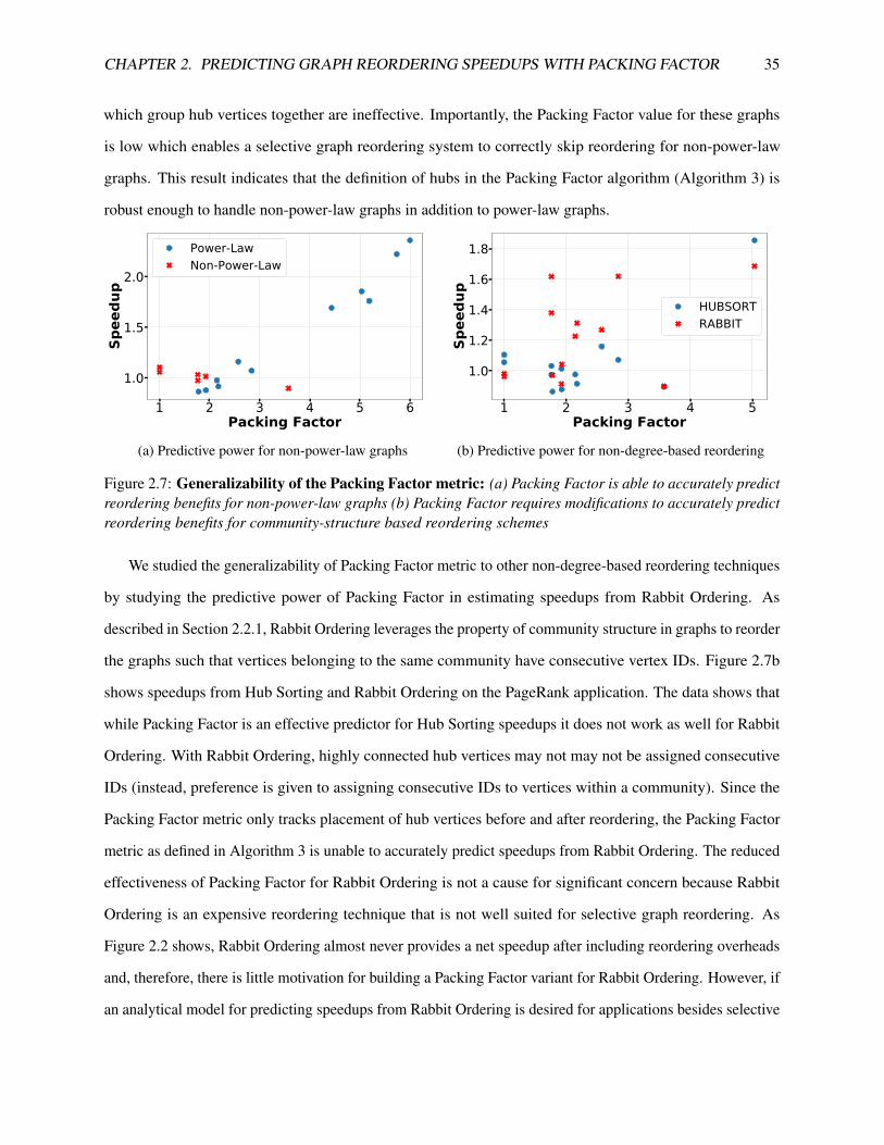
CHAPTER 2. PREDICTING GRAPH REORDERING SPEEDUPS WITH PACKING FACTOR 35
which group hub vertices together are ineffective. Importantly, the Packing Factor value for these graphs
is low which enables a selective graph reordering system to correctly skip reordering for non-power-law
graphs. This result indicates that the definition of hubs in the Packing Factor algorithm (Algorithm 3) is
robust enough to handle non-power-law graphs in addition to power-law graphs.
1 2 3 4 5 6Packing Factor
1.0
1.5
2.0
Spee
dup
Power-LawNon-Power-Law
(a) Predictive power for non-power-law graphs
1 2 3 4 5Packing Factor
1.0
1.2
1.4
1.6
1.8
Spee
dup
HUBSORTRABBIT
(b) Predictive power for non-degree-based reordering
Figure 2.7: Generalizability of the Packing Factor metric: (a) Packing Factor is able to accurately predictreordering benefits for non-power-law graphs (b) Packing Factor requires modifications to accurately predictreordering benefits for community-structure based reordering schemes
We studied the generalizability of Packing Factor metric to other non-degree-based reordering techniques
by studying the predictive power of Packing Factor in estimating speedups from Rabbit Ordering. As
described in Section 2.2.1, Rabbit Ordering leverages the property of community structure in graphs to reorder
the graphs such that vertices belonging to the same community have consecutive vertex IDs. Figure 2.7b
shows speedups from Hub Sorting and Rabbit Ordering on the PageRank application. The data shows that
while Packing Factor is an effective predictor for Hub Sorting speedups it does not work as well for Rabbit
Ordering. With Rabbit Ordering, highly connected hub vertices may not may not be assigned consecutive
IDs (instead, preference is given to assigning consecutive IDs to vertices within a community). Since the
Packing Factor metric only tracks placement of hub vertices before and after reordering, the Packing Factor
metric as defined in Algorithm 3 is unable to accurately predict speedups from Rabbit Ordering. The reduced
effectiveness of Packing Factor for Rabbit Ordering is not a cause for significant concern because Rabbit
Ordering is an expensive reordering technique that is not well suited for selective graph reordering. As
Figure 2.2 shows, Rabbit Ordering almost never provides a net speedup after including reordering overheads
and, therefore, there is little motivation for building a Packing Factor variant for Rabbit Ordering. However, if
an analytical model for predicting speedups from Rabbit Ordering is desired for applications besides selective

CHAPTER 2. PREDICTING GRAPH REORDERING SPEEDUPS WITH PACKING FACTOR 36
reordering, then the primary goal should be to devise an inexpensive way to identify the communities in a
graph (and check whether they are assigned assigned consecutive IDs before and after reordering).
In conclusion, this chapter showed that, after accounting for overheads, graph reordering is not always a
performance optimization (Figure 2.2). Through extensive characterization, we categorized different graph
applications based on their expected benefit from graph reordering (Section 2.3). Finally, we proposed
the Packing Factor metric that accurately predicts benefits from graph reordering (Figure 2.6) and enables
selective graph reordering; essentially ensuring that graph reordering never becomes a performance de-
optimization.

Chapter 3
Improving Locality and Scalability with
RADAR
So far we have looked at the problem of poor cache locality of graph analytics workloads. In the previous
chapter, we saw how Graph Reordering techniques such as Degree Sorting (assigning vertices consecutive
IDs in decreasing order of vertex degrees) helps improve cache locality by improving spatial and temporal
locality of vertex data accesses. In addition to poor cache locality, graph analytics workloads also suffer from
heavy synchronization overheads due to the need to use atomic updates (Section 1.4.2). Data duplication, a
popular approach to eliminate atomic updates by creating thread-local copies of shared data, incurs extreme
memory overheads when applied to graph analytics because of the large sizes of typical input graphs. For
example, a graph with 100 million vertices processed by 32 threads would incur an untenable duplication
overhead of ∼12GB for the shared vertex data (assuming 4 bytes per vertex). Fortunately, the power-law
degree distribution (common in real-world graphs) allows a more memory-efficient data duplication strategy
by duplicating only the highly-connected "hub" vertices. Duplicating only the hub vertex data eliminates
a majority of the atomic updates while avoiding the memory bloat of naive full-graph data duplication.
However, even this memory-efficient data duplication strategy has a lingering source of inefficiency – to
identify whether a vertex is a hub or not. Since the vertex ordering of a graph may be arbitrary, hub vertices
may be spread across the vertex ID space requiring the memory-efficient data duplication implementation to
pay a cost (to determine whether a vertex is a hub) on every update.
The main insight of this work is that the combination of memory-efficient data duplication and Degree
37

CHAPTER 3. IMPROVING LOCALITY AND SCALABILITY WITH RADAR 38
Sorting are mutually enabling optimizations. Degree Sorting optimizes power-law-specific memory-efficient
data duplication by eliminating the costs associated with identifying hub vertices (in a reordered graph, hub
vertices have consecutive IDs in the beginning of the vertex ID space). Data duplication optimizes Degree
Sorting by eliminating any false sharing caused by packing the most heavily-accessed hub vertices in the
same cache line. In this chapter, we present our work called RADAR 1 which combines duplication and
reordering into a single graph analytics optimization, eliminating the costs of both optimizations and reaping
the benefits of each [18]. RADAR improves performance of graph applications by reducing the number
of atomic updates and improving locality of memory accesses, providing speedups of up to 165x (1.88x
on average) across a broad range of graph applications and power-law input graphs. In addition to these
performance improvements, RADAR also offers two other important benefits. First, RADAR eliminates
the cost of atomic updates in graph applications without compromising work-efficiency in contrast to the
state-of-the-art solution for eliminating atomic updates – Push-Pull direction switching [27, 32, 154]. The
Push-Pull optimization avoids atomic updates in graph applications by redundantly processing extra edges,
trading off work-efficiency for a reduction in atomics. Second, by avoiding the need to switch to the pull
mode, RADAR requires only half of the memory footprint of Push-Pull because RADAR only needs to store
the CSR (for push execution) whereas Push-Pull requires storing both the CSR and the CSC. The reduced
memory requirement allows RADAR to process a substantially larger input graph than push-pull, on a single
machine with a fixed memory capacity.
3.1 The Case for Combining Duplication and Reordering
We first quantify the extent to which atomic updates impact the performance of parallel graph applications.
Next, we show the tension between locality improvements from graph reordering (e.g., Degree Sorting) and a
commensurate performance degradation due to false sharing in a parallel execution. These costs motivate
RADAR, which synergistically combines duplication and reordering to reduce atomic updates and improve
cache locality of vertex data accesses.
1Due to the mutually enabling combination of Duplication and Reordering, we name our system RADAR (Reordering AssistedDuplication/Duplication Assisted Reordering)

CHAPTER 3. IMPROVING LOCALITY AND SCALABILITY WITH RADAR 39
3.1.1 Atomics Impose Significant Overheads
Atomic instructions impose a significant penalty on graph applications [20,21,22,31,171,173,174]. Compared
to other kinds of graphs, the performance cost of atomic updates is higher while processing power-law graphs
because the highly-connected hub vertices are frequently updated in parallel. To motivate RADAR, we
experimentally measured the performance impact of atomic updates (evaluation setup in Section 3.3.3). We
compare the performance of a baseline execution with a version that replaces atomic instructions with plain
loads and stores. To ensure that the latter version produces the correct result and converges at the same rate
as the baseline, we execute each iteration twice: once for timing without atomics, and once for correctness
with atomics (but not timed).
PR-Delta BC Radii BFSApplications
0.000.250.500.751.001.251.501.752.00
Sp
eedu
p
BASELINE NO ATOMICS
Figure 3.1: Performance improvement from removing atomic updates in graph applications
Figure 3.1 shows the impact of atomic updates for several applications processing PLD, a power-law
graph. The data show the performance potential of eliminating atomic updates in different applications.
PageRank-Delta (PR-Delta) and Betweenness Centrality (BC) see a large improvement, indicating a high
cost due to atomics. Breadth-first Search (BFS) and Radius Estimation (Radii) see a smaller improvement.
These two algorithms allow applying the Test-and-Test-and-Set optimization [150], which avoids atomics
for already-updated vertices in the baseline. Across the board, the data show the opportunity to improve
performance by eliminating atomic updates.
3.1.2 Data Duplication for Power-law Graphs
Data duplication is a common optimization used in distributed graph processing systems [118], where vertex
state is replicated across machines to reduce inter-node communication. Recent distributed graph processing
systems [40, 72, 143] have leveraged the power-law degree distribution, common to many real world graphs,
to propose data duplication only for the highly connected hub vertices. Duplicating only the hub vertex data
CHAPTER 3. IMPROVING LOCALITY AND SCALABILITY WITH RADAR 40
improves memory efficiency by incurring the overheads of duplication only for the small fraction of hub
vertices (that contribute the most to inter-node communication). In this work, we explore data duplication of
hub vertices in power-law graphs (henceforth referred to as HUBDUP) in the context of single node, shared
memory graph processing to reduce inter-core communication caused by atomic updates. Specifically, we
create thread-local copies of hub vertex data which allows threads to independently update their local copy of
the vertex data without using atomic instructions. Later, threads use a parallel reduction to combine their
copies, producing the correct final result.
The hub-specific duplication strategies proposed in recent distributed graph processing systems [40,
72, 143] cannot be directly applied to the shared memory setting because of fundamental differences in
the primary performance bottlenecks. The primary bottleneck in distributed graph processing is expensive
inter-node communication [152]. To reduce communication over the network, distributed graph processing
systems require sophisticated preprocessing algorithms to effectively partition a graph’s edges across nodes
in addition to duplicating hub vertex data. The high preprocessing costs of these algorithms are harder to
justify in the context of shared memory graph processing due to the relatively low cost of communication
(between cores within a processor). The primary bottleneck in single node, shared memory graph processing
is the latency to access main memory (DRAM) [152, 176]. Therefore, efficient data duplication for shared
memory graph processing must ensure that the increased memory footprint from duplication can be serviced
from the processor’s Last Level Cache (LLC). Otherwise, the performance benefits of eliminating atomic
updates would be overshadowed by an increase in DRAM accesses. The limited capacity of typical LLCs
(order of MBs) allows shared memory graph processing frameworks to duplicate far fewer vertices than
distributed graph processing systems.
Despite the significant overhead imposed by atomic instructions (Figure 3.1), popular shared memory
graph processing frameworks [27,145,154,160] do not use data duplication (including HUBDUP). Achieving
high performance from HUBDUP requires careful implementation to avoid excessive overheads. A key
challenge facing any HUBDUP implementation is that a hub vertex may initially have an arbitrary position
in the vertex data array. A memory-efficient HUBDUP implementation must dynamically identify whether
a vertex being updated is a hub or not at runtime. Consequently, a HUBDUP implementation will remain
sub-optimal; while HUBDUP successfully eliminates atomics for hubs, its incurs a run time cost to identify
those hubs.

CHAPTER 3. IMPROVING LOCALITY AND SCALABILITY WITH RADAR 41
3.1.3 Graph Reordering can Increase False Sharing
Graph analytics workloads are notorious for their poor cache locality [28, 128, 164, 171, 176]. Reordering the
vertices in a graph in decreasing degree order (which we refer to as Degree Sorting) is an effective locality
optimization strategy for graphs with power-law degree distributions. Degree Sorting causes the vertices
with the highest degrees (i.e., hubs) to be assigned at the start of the vertex data array. An access to a hub
vertex’s data also caches the data for the other hubs in the same cache line. Bringing more hubs into the
cache increases the likelihood that future requests to hub vertices hit in the cache, improving performance.
Degree Sorting is appealing because it is a preprocessing step that requires no modification to application
code. While more sophisticated graph ordering techniques exist [34, 92, 164], Degree Sorting has the benefit
of having a relatively low preprocessing overhead. The high preprocessing cost of other approaches negates
the benefit of reordering [13, 17].
PR-Delta BC BFS RadiiApplications
0.000.250.500.751.001.25
Sp
eedu
p
Threads - 1
PUSH
+DEGSORT
PR-Delta BC BFS RadiiApplications
0.000.250.500.751.001.25
Threads - 56
PUSH
+DEGSORT
Figure 3.2: False sharing caused by Degree Sorting: Reordering improves performance of a single-threaded execution but fails to provide speedups for parallel executions.
Figure 3.2 shows the performance improvements offered by reordering vertices in decreasing in-degree
order while processing the PLD power-law graph, for different thread counts. In a single-threaded execution,
Degree Sorting’s locality optimization effectively improves performance. However, in a parallel execution
with 56 threads, Degree Sorting causes a slowdown. False sharing causes the parallel performance degradation,
because Degree Sorting lays the most commonly accessed vertices (hubs) consecutively in memory. As
threads compete to access the cache lines containing these vertices, they falsely share these lines, suffering
the latency overhead of cache coherence activity 2. Single-threaded executions show that Degree Sorting is
effective, but in a highly parallel execution the cost of false sharing exceeds the benefit of Degree Sorting,
leading to performance loss.
2Note that the amount of true sharing is invariant to graph’s vertex ordering and only depends on the structure of the graph.

CHAPTER 3. IMPROVING LOCALITY AND SCALABILITY WITH RADAR 42
3.1.4 Benefits of Combining Duplication and Reordering
The previous sections show that optimizations targeting a reduction in atomic updates and improvement in
cache locality both have limitations. HUBDUP reduces atomic updates but incurs a cost to detect the hub
vertices at runtime. Degree Sorting improves cache locality for a single-threaded execution, but suffers from
false sharing in a parallel execution.
Our main insight in this work is that combining the two optimizations — i.e., HUBDUP on a degree-sorted
graph — alleviates the bottleneck inherent in each. Reordering the input graph in decreasing degree-order
locates hubs contiguously in the vertex array, enabling a HUBDUP implementation to identify the hub
vertices at a lower cost. Duplicating vertex data for hubs eliminates the false-sharing incurred by Degree
Sorting, because each thread updates a thread-local copy of hub vertex data. Table 3.1 shows an overview of
existing techniques with their strengths and weaknesses, including RADAR, the technique we develop in this
work.
Optimization Summary Strengths/WeaknessesHUBDUP Duplicating only hub data + No atomics for hub vertices
(in original graph order) - Cost for identifying the hubsDegree Sorting Reorder graph in decreasing + Improves cache locality
degree order (no app change) - Introduces false sharingRADAR Duplicating only hub data on a
degree sorted graph+ No atomics for hubs (with easy hub detection)
+ Improves cache locality (no false sharing on hub updates)
Table 3.1: Summary of optimizations: RADAR combines the benefits of Degree Sorting and HUBDUPwhile eliminating the overheads of each
3.2 RADAR: Combining Data Duplication and Graph Reordering
RADAR combines the mutually-beneficial HUBDUP and Degree Sorting optimizations, providing better
performance compared to applying either optimization in isolation. To motivate RADAR’s design, we first
describe the space of HUBDUP designs, characterizing the fundamental costs associated with any HUBDUP
implementation. We then discuss how Degree Sorting reduces the inefficiencies of HUBDUP. Finally, we
describe the RADAR implementation that combines reduction in atomic updates with improvements in cache
locality to improve performance of graph applications.

CHAPTER 3. IMPROVING LOCALITY AND SCALABILITY WITH RADAR 43
3.2.1 Sources of Inefficiency in HUBDUP
Power-law graphs present an opportunity to develop memory-efficient data duplication implementations
(HUBDUP). Despite the low memory overhead of duplicating hub vertex data only, HUBDUP’s performance
is sub-optimal. Specifically, implementing HUBDUP requires addressing four key challenges.
Update(vtxData[dst])
Update vtxData[dst]using atomics
1) Find index into threadlocal copies 2) Update local copy without atomics
Y
NIs dst ahub?
(a) Identifying hub verticesvtxData
Map
LocalCopies[tid]
(b) Gathering hub vertex updates in thread-local copies
LocalCopies[0] LocalCopies[N]. . .
Reduce
vtxData
Inv_Map
(c) Reduction of values in thread-local copies
Figure 3.3: HUBDUP design: Essential parts of any HUBDUP implementation. Hub vertices of the graphare highlighted in red.
Challenge #1: Locating hub vertices. Hub vertex data may be arbitrarily located in the vertex data
array, because HUBDUP makes no assumption about input graph ordering. A HUBDUP implementation
must identify whether a vertex is a hub. One possible implementation is to inspect the entire graph in advance
and store an index (i.e., a bitvector) of hub vertex locations.
Challenge #2: Detecting hub vertices. HUBDUP limits memory overheads by duplicating only hub
vertex data. A HUBDUP implementation must dynamically check whether a vertex is a hub or not; hub
updates modify a thread-local copy, while non-hub updates atomically update the vertex data array. An
implementation can use the bitvector mentioned above to efficiently make this hub check on every vertex
update at run time, as illustrated in Figure 3.3a
Challenge #3: Updating the thread-local hub copies. Hub updates in HUBDUP are applied to a
thread-local copy of the hub’s data and do not use atomic instructions. A memory efficient HUBDUP
implementation must store hub duplicates contiguously in memory (e.g., LocalCopies in Figure 3.3b).
However, packing hub vertices in thread-local copies precludes using a hub vertex’s ID as an index to the
thread-local copies. HUBDUP requires mapping a hub vertex’s ID to its index in the thread-local copies (as
CHAPTER 3. IMPROVING LOCALITY AND SCALABILITY WITH RADAR 44
in Figure 3.3b). The mapping function must be called on every hub update as shown in Figure 3.3a.
Challenge #4: Reducing updated hub copies. At the end of an iteration, partial hub updates accumu-
lated in thread-local copies must be reduced and stored in the hub’s entry in the vertex data array (Figure 3.3c).
Locating a hub copy’s original location in the vertex array requires an inverse mapping from its index in the
array of thread-local copies back to its index in the original vertex data array.
A key motivation for RADAR is achieving the benefits of HUBDUP without incurring the costs of the
above challenges.
3.2.2 Degree Sorting Improves HUBDUP
Degree Sorting improves HUBDUP by reducing the costs associated with each challenge. Most of the cost
of HUBDUP stems from the arbitrary location of hubs in the vertex data array. Degree Sorting solves this
problem by arranging vertices in decreasing in-degree order. A degree-sorted graph avoids the first two
challenges: identifying a hub requires simply checking that its index is lower than a constant threshold
index marking the boundary of hub vertices. Indexing thread-local copies is also simple because hubs are
contiguous. A hub’s vertex ID can be used to directly index into the thread-local copies. Therefore, Degree
Sorting eliminates the cost of building and accessing the maps and inverse maps from challenges #3 and #4.
3.2.3 HUBDUP Improves Degree Sorting
Degree Sorting improves cache locality by tightly packing high-degree hubs in the vertex data array. Figure 3.2
demonstrates the benefit of locality improvements for single-threaded graph applications. However, contiguity
of hubs causes an unnecessary increase in costly false sharing because different threads frequently read and
update the small subset of cache lines containing hubs. Thread-local hub copies in HUBDUP avoid false
sharing because a thread’s hub updates remain local until the end of an iteration.
3.2.4 RADAR = HUBDUP + Degree Sorting
RADAR combines the best of HUBDUP and Degree Sorting by duplicating hub vertex data in a degree sorted
graph. Duplication mitigates false sharing and degree sorting keeps the overhead of duplication low. The key
motivation behind RADAR is the observation that HUBDUP and Degree Sorting are mutually enabling. The

CHAPTER 3. IMPROVING LOCALITY AND SCALABILITY WITH RADAR 45
key contribution of RADAR is the tandem implementation of these techniques, which realizes their mutual
benefits.
3.2.5 Implementation Details
We now describe the low-level implementation details and optimizations of RADAR. We also cover the imple-
mentation details of a HUBDUP baseline because, to the best of our knowledge, an efficient implementation
of HUBDUP does not exist in the literature.
HUBDUP design decisions: We designed and implemented HUBDUP with the aim of keeping the
space and time overheads of duplication low. To identify hubs (challenge #1) we collect the in-degrees of
all vertices and then sort the in-degrees to find the threshold degree value for a vertex to be classified as a
hub. We use GCC’s __gnu_parallel::sort to sort indices by degree efficiently. Note that sorting indices
is much simpler than re-ordering the graph according to the sorted order of indices (Degree Sorting). We
use the hMask bitvector to dynamically detect hubs (i.e., challenge #2), setting a vertex’s bit if its degree is
above a threshold. hMask has a low memory cost: a 64M-vertex graph requires an 8MB bitvector to track
hubs, which is likely to fit in the Last Level Cache (LLC). We use an array to implement the mapping from a
hub’s vertex ID to its index into the thread-local copies and another array for the inverse mapping. HUBDUP
populates both arrays in advance.
Optimizing reduction costs: After each iteration, both HUBDUP (and RADAR) must reduce updated
thread-local hub copies and store each hub’s reduction result in its entry in the vertex array. Only a subset
of hub vertices may need to be reduced in a given iteration because frontier-based applications update the
neighbors of vertices in the frontier only (Algorithm 1). An efficient implementation of HUBDUP should
avoid reducing and updating hubs that were not updated during that iteration. HUBDUP and RADAR
explicitly track an iteration’s updated hub vertices with a visited array that has an entry for each hub. An
update to a hub (by any thread) sets the corresponding entry in the visited using the Test-and-Test-and-Set
operation (if a hub’s visited bit is set once in an iteration, it is never set again until the next iteration). After
an iteration, HUBDUP reduces the thread-local, partial updates of each hub that has its visited entry set
and does nothing for other hubs. This visited optimization to reduction improved RADAR performance by
up to 1.25x (geometric mean speedup of 1.02x).

CHAPTER 3. IMPROVING LOCALITY AND SCALABILITY WITH RADAR 46
Selecting hub vertices for duplication: Due to limited Last Level Cache (LLC) capacity, duplicating
all the hubs 3 in a graph may impose excessive memory overheads. Instead of duplicating all hubs, HUBDUP
and RADAR should duplicate only a subset of hubs (hub vertices with the highest degrees) such that the sum
of the sizes of all threads’ duplicates is less than the capacity of the LLC (Last Level Cache). We demonstrate
the importance of duplicating only a subset of hubs by comparing our LLC-capacity-guided duplication
strategy (“CACHE-RADAR”) to a variant that duplicated all hubs (“ALL-HUBS-RADAR”). Figure 3.4
shows their relative performance running all applications on DBP, the smallest graph in our dataset. The data
show that CACHE-RADAR consistently outperforms ALL-HUBS-RADAR, with better LLC locality for
all threads’ hub duplicates. The performance gap is likely to grow with graph size, as more hub duplicates
compete for fixed LLC space. Our CACHE-RADAR design most effectively uses the scarce LLC space to
keep only the highest-degree hubs’ duplicates cached.
PR PR-Delta Local-TriCnt BC BFS RadiiApplications
0.000.250.500.751.001.251.501.752.00
Sp
eedu
p
Graph - DBP
PUSH
+ALL-HUBS-RADAR
+CACHE-RADAR
Figure 3.4: Performance of RADAR with different amounts of duplicated data: The duplication over-head of ALL-HUBS-RADAR are significant even for the smallest input graph.
numHubs =S∗LLC_Size
(T ∗ elemSz)+ δ(3.1)
This result demonstrates the importance of calibrating HUBDUP and RADAR to the properties of the
machine (LLC size). We use Equation 1 to calculate the number of hubs to duplicate in HUBDUP and
RADAR. S is a scaling factor (between 0 and 1) that controls the fraction of LLC to be reserved for storing
duplicated data, T is the number of threads used, and elemSz is the size (in bytes) of each element in the
vertex data array. The δ parameter in the denominator of Equation 1 accounts for memory overheads in
HUBDUP and RADAR. Both RADAR and HUBDUP use a visited boolean array to optimize reduction
(Section 3.2.5). We set δ = 1, because the visited array has an entry for each hub. For HUBDUP,
maintaining the hMask bitvector and maps to and from a hub’s duplicate’s location are additional memory
3As in prior work [176], a hub is defined as a vertex with degree greater than the average degree.

CHAPTER 3. IMPROVING LOCALITY AND SCALABILITY WITH RADAR 47
costs and we set δ = 3. On varying the S parameter, we empirically determined that S = 0.9 often provided
the best performance across applications and graphs.
3.3 Performance Improvements with RADAR
This section evaluates the speedups from RADAR on a range of graph applications and input graphs. We first
describe our graph applications, input graphs, and evaluation setup before showing RADAR’s performance
results.
3.3.1 Graph Applications
We evaluate the performance of RADAR 4 across five applications from the Ligra benchmark suite [154] and
one application from the GAP [27] benchmark suite. All the applications were compiled using g++-6.3 with
-O3 optimization level and use OpenMP for parallelization. We provide a brief description of the execution
characteristics of each application, identifying the vertex data array and atomic update operation performed
on vertex data.
PageRank (PR): PR is a popular graph benchmark that iteratively refines per-vertex ranks (vertex data)
until the sum of all ranks drops below a convergence threshold. The application processes all the vertices in
a graph every iteration and, hence, performs many random writes to the vertex data array. PR uses atomic
instructions to increment vertex ranks of destination vertices based on properties of neighboring source
vertices.
PageRank-delta (PR-Delta): PR-Delta is a variant of PageRank that does not process all the vertices of
a graph each iteration. Instead, PR-Delta only processes a subset of vertices for which the rank value changed
beyond a δ amount, which improves convergence [118]. Even though PR-Delta does not process all vertices
every iteration, the application processes dense frontiers during the initial iterations of the computation which
generate many random writes to the vertex data array. PR-Delta uses atomic instructions in a similar fashion
to PR.
Betweenness Centrality (BC): BC iteratively executes a BFS kernel from multiple sources to count the
number of shortest paths passing through each vertex (vertex data). Most iterations of BC process sparse
frontiers (i.e. frontier contains a small fraction of total vertices). BC also performs a transpose operation
4Source code for RADAR (and all the other optimizations) is available at https://github.com/CMUAbstract/RADAR-Graph

CHAPTER 3. IMPROVING LOCALITY AND SCALABILITY WITH RADAR 48
(exchanging incoming neighbors with outgoing neighbors and vice versa) and, hence, is an application that
needs to store two CSRs even in a baseline push-based execution. BC uses atomic instructions to increment
the number of shortest paths passing through each vertex.
Radii Estimation (Radii): Graph Radii estimation approximates the diameter of a graph (longest
shortest path) by performing simultaneous BFS traversals from many randomly-selected sources. Radii uses
a bitvector (vertex data) to store information about BFS traversals from multiple source vertices. Atomic
instructions are used to atomically perform a bitwise-OR on the vertex data array. Unlike applications
discussed so far, subsequent updates to the vertex data array might produce no change to the vertex data array.
Therefore, Radii uses the Test-and-Test-and-Set (T&T&S) optimization [150] to avoid executing atomic
instructions for updates that will produce no change.
Breadth First Search (BFS): BFS is an important graph processing kernel that is often used as a
subroutine in other graph algorithms. The kernel iteratively visits all the neighbors reachable from a particular
source, identifying a parent for each vertex (vertex data). Similar to Radii, BFS also uses the T&T&S
optimization to atomically set a parent for each vertex.
Local Triangle Counting (Local-TriCnt): Local Triangle Counting identifies the number of triangles
(or cliques of size 3) incident at each vertex (vertex data) of an undirected graph and is a variant of the
Triangle Counting benchmark that only reports the total count of triangles. Our Local-TriCnt implementation
extends the optimized Triangle Counting implementation from GAP which performs Degree Sorting on
the input graph to achieve an algorithmic reduction in the number of edges to be processed. Finding the
number of triangles per-vertex allows computing a graph’s local clustering coefficients which has applications
in identifying tightly-knit communities in social networks [56]. Local-TriCnt uses atomic instructions to
increment the number of triangle discovered for each vertex.
3.3.2 Input graphs
To evaluate RADAR’s performance, we use large, real-world, power-law input graphs that have been
commonly used in other academic research. We also include the kronecker synthetic graph in our evaluation
due to their popularity in the graph500 community [133]. Table 3.2 lists key statistics for the graphs in our
dataset. Unless noted otherwise, we use the original vertex data ordering of the input graph as provided by
the authors of the graph dataset for our baseline executions.

CHAPTER 3. IMPROVING LOCALITY AND SCALABILITY WITH RADAR 49
DBP GPL PLD TWIT MPI KRON WEB SD1Reference [103] [71] [126] [104] [103] [27] [51] [126]|V | (in M) 18.27 28.94 42.89 61.58 52.58 67.11 50.64 94.95|E| (in B) 0.172 0.462 0.623 1.468 1.963 2.103 1.93 1.937Avg. Degree 9.4 16 14.5 23.8 37.3 31.3 38.1 20.4% of Hubs 11.75 20.54 14.72 11.30 9.52 8.43 5.56 10.61
Table 3.2: Statistics for the evaluated input graphs
3.3.3 Evaluation Platform and Methodology
We performed all of our experiments on a dual-socket server machine with two Intel Xeon E5-2660v4
processors. Each processor has 14 cores, with two hardware threads each, amounting to a total of 56 hardware
execution contexts. Each processor has a 35MB Last Level Cache (LLC) and the server has 64GB of DRAM
provided by eight DIMMs. All experiments were run using 56 threads and we pinned the software thread to
hardware threads to avoid performance variations due to OS thread scheduling. To further reduce sources of
performance variation, we also disabled the “turbo boost” DVFS features and ran all cores at the nominal
frequency of 2GHz.
We ran 4 trials for the long-running applications (PageRank and Local Triangle Counting) in our
evaluation set, and 11 trials for all the other applications. While computing the mean time, we exclude the
timing for the first trial to allow processor caches to warm up. For the source-dependent BFS application, we
select a source vertex belonging to the largest connected component in the graph. We maintain a mapping
between vertex IDs before and after reordering to ensure that source-dependent applications running on the
reordered graphs use the same source as a baseline execution on the original graph [27].
3.3.4 Performance Analysis of RADAR
To illustrate the benefits of combining HUBDUP and Degree Sorting, we compare RADAR’s performance
with executions that either perform HUBDUP or Degree Sorting. Figure 3.5 shows the performance of
HUBDUP, Degree Sorting, and RADAR relative to a baseline, push-style execution of graph applications
across 8 input graphs. We report the key findings from the results below:
Finding 1: RADAR outperforms HUBDUP and Degree Sorting. For PR, PR-Delta, Local-TriCnt,
and BC, RADAR consistently provides higher speedups than only performing HUBDUP or Degree Sorting.
The results highlight the synergy between HUBDUP and Degree Sorting which is exploited by RADAR to
provide additive performance gains.

CHAPTER 3. IMPROVING LOCALITY AND SCALABILITY WITH RADAR 50
DBP GPL PLD TWIT MPI KRON WEB SD1 GMEAN0.00.51.01.52.02.5
Sp
eedu
p12x 26x
PR
DBP GPL PLD TWIT MPI KRON WEB SD1 GMEAN0.00.51.01.52.02.5
9.7x 19x
PR-Delta
DBP GPL PLD TWIT MPI KRON WEB SD1 GMEAN0.0
2.0
4.0
6.0
8.0
Sp
eedu
p 8.9x 64x 14x 165x 9.5x
Local-TriCnt
DBP GPL PLD TWIT MPI KRON WEB SD1 GMEAN0.00.51.01.52.02.53.0
BC
DBP GPL PLD TWIT MPI KRON WEB SD1 GMEANInput Graphs
0.00.51.01.52.02.5
Sp
eedu
p
BFS
DBP GPL PLD TWIT MPI KRON WEB SD1 GMEANInput Graphs
0.00.51.01.52.02.5
Radii
PUSH +HUBDUP +DEGSORT +RADAR
Figure 3.5: Comparison of RADAR to HUBDUP and Degree Sorting: RADAR combines the benefits ofHUBDUP and Degree Sorting, providing higher speedups than HUBDUP and Degree Sorting applied inisolation.
Finding 2: HUBDUP offers speedup in graphs with good ordering of hubs. For the four applications
mentioned above, HUBDUP only provides speedups on three input graphs - DBP, MPI, and WEB - often causing
a slowdown for the other input graphs. HUBDUP performs well in the DBP, MPI, and WEB graphs because
most hub vertices are consecutively ordered in these graphs. Due to the consecutive ordering of hub vertices,
accesses to key HUBDUP data structures – the hMask bitvector and the mapping from hub vertex ID to
locations in thread-local copies – benefit from improved locality, driving down the costs of an HUBDUP
execution.DBP GPL PLD TWIT MPI KRON WEB SD1
PR Speedup 2.06x 0.85x 0.84x 0.86x 1.49x 0.62x 11.91x 0.90xUnique words 17.03K 22.39K 64.32K 68.80K 13.03K 71.38K 6.02K 53.56
Table 3.3: Number of unique words in the hMask bitvector containing hub vertices: HUBDUP offersthe highest speedups for graphs in which hubs map to the fewest number of unique words in the bitvector.
Table 3.3 demonstrates the relation between HUBDUP performance and the vertex order of the graph
by showing speedup from HUBDUP for PageRank (PR) along with the number of unique words in the
hMask bitvector corresponding to hub vertices. For the same number of hubs (a machine-specific property as
described in Section 3.2.5), hubs in the DBP, MPI, and WEB graphs map to fewer words in the hMask bitvector
(an 8B word in the bitvector encodes information for 64 vertices). Fewer words associated with hub vertices
improves locality of hMask accesses and allows HUBDUP to provide speedups. The results indicates that
HUBDUP is likely to provide speedups for input graph orderings where hub vertices have nearly consecutive
IDs.

CHAPTER 3. IMPROVING LOCALITY AND SCALABILITY WITH RADAR 51
Finding 3: Degree Sorting can lead to performance degradation. Degree Sorting causes slowdowns
in PR, PR-Delta, and BC for certain input graphs. Section 3.1.3 showed that the performance degradation is
due to increased coherence traffic caused by false sharing between threads updating hub vertex data. The
slowdown from increased coherence traffic is higher for applications that update more vertices each iteration
(PR and PR-Delta) because these applications have a higher likelihood of simultaneously updating hub
vertices from different threads. RADAR provides speedups in these applications by duplicating hub vertex
data to avoid an increase in coherence traffic.
Finding 4: Degree Sorting provides significant speedups for Local-TriCnt. The results for the PLD,
TWIT, and WEB graphs on Local-TriCnt show high speedups from Degree Sorting. The high speedups are
due to an algorithmic reduction in the number of edges that need to be processed to identify all the triangles
in the graph. The GAP implementation of Triangle Counting already uses Degree Sorting. We normalize
data to a baseline without Degree Sorting to show the algorithmic improvement from reordering. RADAR
provides additional speedups over the algorithmic improvements from Degree Sorting by eliminating atomic
instructions, improving performance by 4.7x on average over Degree Sorting.
Finding 5: Degree Sorting performs best for BFS and Radii. In contrast to Finding 1, the results for
BFS and Radii show that Degree Sorting consistently outperforms RADAR and HUBDUP. BFS and Radii
use the Test-and-Test-and-Set (T&T&S) optimization, which reduces the cost of atomic updates for these
applications (Figure 3.1). The T&T&S optimization also helps avoid an increase in coherence traffic from
Degree Sorting, thereby improving locality. For BFS and Radii, the small improvements from eliminating
atomic updates do not justify the cost of duplicating hub vertex data causing RADAR to provide lower
performance that Degree Sorting.
DBP GPL PLD TWIT MPI KRON WEB SD1Input Graphs
0.0
0.5
1.0
1.5
2.0
Sp
eedu
p
22.2xBFS (No T&T&S)
PUSH +DEGSORT +RADAR
Figure 3.6: Performance improvements for BFS without the T&T&S optimization: In the absence ofthe T&T&S optimization, RADAR outperforms Degree Sorting.
To demonstrate the relation between reduced speedup from RADAR and the T&T&S optimization, we

CHAPTER 3. IMPROVING LOCALITY AND SCALABILITY WITH RADAR 52
studied a BFS implementation that does not use T&T&S. Figure 3.6 shows the performance of Degree Sorting
and RADAR for such a BFS implementation. In the absence of T&T&S, the performance results for BFS
mirror the results for PR and PR-Delta applications, showing slowdowns with Degree Sorting and speedups
with RADAR. While BFS and Radii would never be implemented without the T&T&S optimization, this
experiment was useful for showing that RADAR is most effective for applications that cannot use T&T&S.
3.4 Advantages of Using RADAR Compared to Push-Pull
RADAR combines the benefits of HUBDUP and Degree Sorting and outperforms either optimization applied
in isolation (Figure 3.5). In this section, we discuss the two advantages offered by RADAR over the
current state of the art for eliminating atomic updates in graph analytics workloads – Push-Pull direction
switching [27, 32, 154]. First, in contrast to Push-Pull, RADAR eliminates a majority of the atomic updates
without impacting the work-efficiency of graph applications. Second, RADAR incurs only half the memory
footprint of Push-Pull optimization, allowing RADAR to support larger input graphs with the same memory
budget. We end this section by comparing the preprocessing overheads incurred by RADAR relative to the
Push-Pull optimization.
3.4.1 RADAR’s Work-efficiency Benefits over Push-Pull
Figure 3.7 shows the speedups from RADAR and Push-Pull relative to a baseline, push-based execution.
The results show speedups both including the preprocessing overheads (solid bars) and without including
the cost of preprocessing (total bar height). In this section, we explain the performance of Push-Pull and
RADAR without considering preprocessing overheads (i.e., here we focus on the total bar height) and defer
the discussion on performance with preprocessing costs to Section 3.4.3. The relative benefit of RADAR
over Push-Pull is application-dependent and we report our findings for each application below.
PageRank: PageRank updates every vertex each iteration (i.e. frontier includes all the vertices). There-
fore, every iteration uses the pull phase (Algorithm 2) to eliminate atomic updates. The results show that
executing PR using the pull phase improves performance by eliminating atomic updates. However, RADAR
outperforms the pull-phase execution because RADAR couples eliminating atomic updates for hub vertices
with improved locality. The only exception is the WEB graph which receives significantly higher speedup

CHAPTER 3. IMPROVING LOCALITY AND SCALABILITY WITH RADAR 53
DBP GPL PLD TWIT MPI KRON WEB SD1 GMEAN0.00.51.01.52.02.5
Sp
eedu
p116x89x
26.5x26x
PR
DBP GPL PLD TWIT MPI KRON WEB SD1 GMEAN0.00.51.01.52.02.5 31x
14.8x19x15.6x
PR-Delta
DBP GPL PLD TWIT MPI KRON WEB SD1 GMEAN0.0
2.0
4.0
6.0
8.0
Sp
eedu
p
64x45x
165x140x
9.5x8.8x
Local-TriCnt
DBP GPL PLD TWIT MPI KRON WEB SD1 GMEAN0.00.51.01.52.02.53.0
BC
DBP GPL PLD TWIT MPI KRON WEB SD1 GMEANInput Graphs
0.00.51.01.52.02.5
Sp
eedu
p
3.1x 5xBFS
DBP GPL PLD TWIT MPI KRON WEB SD1 GMEANInput Graphs
0.00.51.01.52.02.5
Radii
PUSH PUSH-PULL +RADAR
Figure 3.7: Speedups from Push-Pull and RADAR: The total bar height represents speedup withoutaccounting for the preprocessing costs of Push-Pull and RADAR. The filled, lower bar segment shows the netspeedup after accounting for the preprocessing overhead of each optimization. The upper, hashed part of thebar represents the speedup loss as a result of accounting the preprocessing overhead of each optimization.
from Push-Pull because the creators of the graph use a sophisticated algorithm [34], that optimizes pull phase
execution, to pre-order the graph at great computational cost [13].
PageRank-delta: PageRank-delta uses the Push-Pull optimization to process the graph in the pull
phase during dense frontiers (i.e. frontier contains most of the vertices in the graph) and in the push phase
otherwise. A pull phase execution eliminates all atomic updates at the expense of reducing work-efficiency.
Additionally, a pull phase execution also converts the regular accesses to the Frontier in the push phase (line
1 in Algorithm 1) into irregular accesses (line 3 in Algorithm 2). For many graphs, the performance loss from
irregular Frontier accesses offsets the benefits from eliminating atomic updates and a Push-Pull execution
causes slowdowns. In contrast, RADAR provides better performance by eliminating a large fraction of atomic
updates while maintaining regular accesses to the Frontier. As before, the WEB graph is an exception,
where the pull-optimized layout of the graph ensures good locality for Frontier accesses. Consequently,
Push-Pull eliminates atomic updates without incurring a penalty for Frontier accesses, leading to significant
performance improvement for the WEB graph.
We explored the trade-off of a pull phase execution, which is to eliminate atomic updates at the expense
of making Frontier accesses irregular, by running PR-Delta on the same graphs but with two different vertex
orders – random ordering and a pull phase optimized ordering called frequency based clustering [176].
Figure 3.8 shows the speedups from Push-Pull and RADAR on graphs with the two different orderings.
Results for the randomly-ordered graphs show that Push-Pull consistently causes slowdowns because the

CHAPTER 3. IMPROVING LOCALITY AND SCALABILITY WITH RADAR 54
DBP GPL PLD TWIT MPI KRON WEB SD10.0
0.5
1.0
1.5S
pee
dup
RANDOM ORDERING
DBP GPL PLD TWIT MPI KRON WEB SD1Input Graphs
0.00.51.01.52.0
Sp
eedu
p
7.6x 6.6xFREQUENCY BASED CLUSTERING
PUSH PUSH-PULL +RADAR
Figure 3.8: Speedups for PR-Delta from Push-Pull and RADAR on graphs with different orderings:Push-Pull causes consistent slowdowns when running on randomly ordered graphs.
random ordering makes Frontier accesses highly irregular, thereby offsetting any performance benefits from
eliminating atomics. Note that Push-Pull causes slowdown even in the WEB graph when it is randomly
ordered. Push-pull performs better for the graphs ordered with the pull-phase optimized frequency based
clustering algorithm. In contrast to Push-Pull, RADAR improves performance regardless of the original
vertex order of the graph and, hence, is more generally applicable.
Local Triangle Counting: Local Triangle Counting operates on undirected ("symmetrized") versions
of input graphs and performs the same accesses in both push and pull phases. For applications like Local
Triangle Counting that operate on undirected graphs, RADAR is the only option for improving performance
by eliminating atomic instructions.
Algorithm 4 Pseudocode for push-phase of BC
1: par_for src in Frontier do2: for dst in out_neigh(src) do3: if Visited[dst] is True then4: AtomicUpd (vtxData[dst]), auxData[src])
Betweenness-Centrality: Just like PageRank-delta, BC uses the Push-Pull optimization by processing
dense frontiers using the pull phase and otherwise using the push phase. However, the per-edge computation
performed in BC (shown in Algorithm 4) is different from PR-Delta. BC performs an additional check on
a Visited data structure (line 3) before performing its per-edge computation. For each edge, BC accesses
two data structures, each indexed by the source and destination IDs of the edge. Regardless of whether
an iteration is processed using the push phase or the pull phase, BC performs irregular accesses to one of
the data structures (Visited during the push phase and Frontier during the pull phase). Therefore, unlike

CHAPTER 3. IMPROVING LOCALITY AND SCALABILITY WITH RADAR 55
PR-Delta, a pull-phase iteration in BC eliminates atomic updates without introducing irregular accesses. As a
result, Push-Pull often outperforms RADAR for BC.
BFS: The Push-Pull direction-switching optimization was originally designed for BFS [27, 154]. In BFS,
processing a dense frontier in the pull-phase allows breaking out of the iteration sooner than a push-phase
execution. Therefore, Push-Pull significantly outperforms RADAR by achieving an algorithmic reduction in
the total number of edges required to be processed.
Radii: Radii has an access pattern similar to PageRank-Delta. However, unlike PageRank-Delta, Radii is
not bottlenecked by atomic updates thanks to T&T&S. With little potential for performance improvement
from eliminating atomic updates (Figure 3.1), Push-Pull provides low speedup for Radii.
3.4.2 Reduced Memory Footprint with RADAR
The Push-Pull optimization doubles an application’s memory footprint. Push-Pull implementations switch
between executing a graph using push and pull phases based on frontier density and, hence, require two
CSRs - one for outgoing neighbors (used during the push phase) and another for incoming neighbors (used
during the pull phase). The higher memory footprint of Push-Pull cuts in half the maximum graph size that
can be processed using a single machine.
PR PR-Delta BFS Radii Local-TriCntInput Graphs
0.000.250.500.751.001.251.501.752.00
Sp
eedu
p
OO
MO
OM
OO
MO
OM
OO
MO
OM
OO
MO
OM
9.6x
SDH Graph (102M vertices, 2B edges)
PUSH PUSH-PULL +RADAR
Figure 3.9: Speedups from RADAR for the SDH graph: RADAR provides speedups while the size of SDHgraph precludes applying the Push-Pull optimization.
To illustrate the limitations imposed by the higher memory footprint of Push-Pull, we ran experiments on
the subdomain host [126] (SDH) graph which is even larger than the SD1 graph. The size of the SDH graph
causes an Out of Memory (OOM) error in our 64GB server when storing both the in- and out- CSRs of the
graph, making it impossible to apply the Push-Pull optimization for the graph. In contrast, our server fits just
the out-CSR of the graph, accommodating the baseline and RADAR versions of applications. Figure 3.9
shows the performance of RADAR on the SDH graph across different applications. We were unable to

CHAPTER 3. IMPROVING LOCALITY AND SCALABILITY WITH RADAR 56
run any configuration for BC since even the baseline execution of BC requires both the in- and out-CSRs.
The result shows that RADAR provides significant performance improvements for the SDH graph, while
Push-Pull runs out of memory. By maintaining the same memory footprint as the baseline, RADAR provides
performance improvements for larger graphs than Push-Pull, making RADAR a more effective optimization
for graph processing in a single, memory-limited machine.
3.4.3 Preprocessing Overheads
All the optimizations covered in the paper – HUBDUP, Degree Sorting, RADAR, and Push-Pull– require
some form of preprocessing on the input graph. The input graph used in Ligra is an adjacency file that stores
outgoing edges of the graph in the CSR format. The preprocessing step for Push-Pull builds an in-CSR (CSR
for incoming edges) by traversing the input graph to first collect all the incoming edges of the graph and then
sorting all the incoming edges by destination IDs. For HUBDUP, the preprocessing step involves populating
the hMask bitvector for identifying hubs and creating maps between hub vertex IDs and unique locations
in thread-local copies of hub data. For RADAR and Degree Sorting, the input graph needs to reordered
in decreasing order of degrees. Reordering the graph requires sorting the in-degrees of vertices to create a
mapping from original vertex IDs to new IDs (ordered by decreasing in-degrees) followed by populating
a new out-CSR with vertices in the new order. Table 3.4 lists the preprocessing algorithm complexity and
runtime for the different optimizations on all input graphs. HUBDUP has the lowest complexity because
it only scans the degrees of all vertices. Push-Pull incurs the maximum complexity because it sorts all the
edges to build an in-CSR. Push-Pull, however, incurs zero preprocessing cost for undirected graphs because
these graphs have the same incoming and outgoing edges. Finally, RADAR imposes lower preprocessing
overhead than Push-Pull for directed graphs.
Complexity DBP GPL PLD TWIT MPI KRON WEB SD1HUBDUP O(V ) 0.06s 0.11s 0.14s 0.24s 0.22s 0.23s 0.19s 0.37sDegSort/RADAR O(V logV +E) 0.88s 2.37s 2.29s 8.26s 19.06s 2.94s 3.49s 7.42sPush-Pull O(ElogE) 2.96s 7.03s 3.91s 9.68s 47.71s 0s 10.86s 12.51s
Table 3.4: Preprocessing costs for HUBDUP, RADAR, and Push-Pull: Degree Sorting and RADAR havea smaller preprocessing cost compared to Push-Pull. (V - #vertices and E - #edges)
Figure 3.7 shows the speedups from Push-Pull and RADAR after accounting for the above preprocessing
costs (filled, lower bar segments). Preprocessing overheads are easily justified for long-running applications
such as PageRank and Local Triangle Counting where RADAR provides a net speedup even after including

CHAPTER 3. IMPROVING LOCALITY AND SCALABILITY WITH RADAR 57
the preprocessing costs. Preprocessing imposes significant overheads for PR-Delta and Radii. However, these
applications are refinement-based algorithms where preprocessing can be justified when more refined results
are desired (for example, lower convergence threshold in PR-Delta, traversals from more sources in Radii
and BC). Finally, preprocessing overheads can be justified for BFS in scenarios where multiple traversals on
the same graph are performed.
3.5 Related Work
We divide the prior work in graph processing related to RADAR into three categories – data duplication,
reducing cost of atomic updates, and locality optimizations.
Data duplication in graph applications: Prior work in distributed graph processing has proposed data
duplication for hub vertices in power-law graphs [72, 143]. Vertex delegates [143] replicates hub vertex data
across all nodes in a cluster and uses asynchronous broadcasts and reductions to reduce total communication
for updating hub data. Powergraph [72] creates replicas of hub vertices to create balanced vertex cuts
(assigning equivalent number of edges to each node). As discussed in Section 3.1.2, the duplication strategies
used in the above systems are not directly applicable in the shared memory setting due to differences in the
primary bottlenecks of the two scenarios. Data duplication has also been used for reducing the cost of atomic
updates in GPU-based graph processing [120]. Similar to RADAR, Garaph highlights the importance of
restricting duplication overheads to avoid an increase in DRAM accesses. However, RADAR and Garaph use
different techniques to reduce duplication overhead. RADAR creates a per-thread copy only for hub vertices
whereas Garaph duplicates all vertices but creates fewer copies than number of threads. The duplication
strategy of Garaph is tied to the out-of-core [105] execution model that targets graphs that cannot fit in
memory and, hence, is orthogonal to RADAR (which targets in-memory graph processing).
Reducing cost of atomic updates: Prior work has proposed techniques to reduce the cost of atomic updates
in graph processing. AAM [31] is a system that uses Hardware Transactional Memory (HTM) to reduce the
cost of atomic updates. AAM amortizes the cost of providing atomicity by applying updates for multiple
vertices within a single transaction instead of atomically updating each vertex. However, the authors report
that AAM is only effective for applications that employ the T&T&S optimization (particularly BFS) and
leads to many transaction aborts for applications that cannot employ T&T&S. Therefore, AAM and RADAR
are complimentary optimizations because RADAR provides the best performance for applications that cannot
CHAPTER 3. IMPROVING LOCALITY AND SCALABILITY WITH RADAR 58
employ T&T&S. Galois [145] uses speculative parallelism to avoid fine grained synchronization and improve
locality in irregular applications. RADAR also aims to avoid fine grain synchronization and improve locality,
but uses data duplication to achieve the goal. Finally, Besta et. al. [32] proposed the "Partition Awareness
(PA)" optimization for reducing atomic updates in push-based graph applications. The PA optimization
creates two CSRs – one identifying neighbors local to a core and another identifying neighbors belonging to
remote cores – allowing threads to update local neighbors without atomic instructions. However, PA requires
static partitioning of vertices to thread and precludes dynamic load balancing (which is critical for power-law
graphs).
Locality optimizations for graph processing: Extensive research in graph reordering has produced re-
ordering techniques with varying levels of sophistication to improve graph locality [13, 34, 92, 164, 176].
While RADAR could potentially be applied with different reordering techniques, efficient duplication of
hub vertices requires that the reordering mechanism produce a graph where the hub vertices are assigned
consecutive IDs (Section 3.2.1). We chose Degree Sorting in our study because of its low overhead and the
advantage of assigning hub vertices consecutive IDs at the start of the vertex array. Studying combinations of
RADAR with different reordering techniques is an interesting line of research and we leave this exploration
for future work.
Vertex scheduling is an alternative to graph reordering that improves locality by changing the order of
processing vertices. Prior work [125,176] has shown that traversing the edges of a graph along a Hilbert curve
can improve locality of graph applications. However, these techniques complicate parallelization [28, 176].
Vertex scheduling only targets an improvement in locality and, unlike graph reordering, does not help in
improving the efficiency of data duplication for power-law graphs.
Cache blocking is another technique used to improve locality of graph applications. Zhang et. al. [176]
proposed CSR segmenting – a technique to improve temporal locality of vertex data accesses by breaking the
original graph into subgraphs that fit within the Last Level Cache. Propagation blocking [28, 37] partition
updates to vertex data instead of partitioning the graph. RADAR differs from these prior works in that
RADAR targets not just locality improvement but also a reduction in atomic updates.
Graph partitioning techniques, traditionally used for reducing communication in distributed graph
processing, have recently been applied to improve locality of in-memory graph processing frameworks [158,
159, 175]. Sun et. al. [158] proposed a partitioning approach where all the incoming edges of a vertex
are placed in the same partition to improve temporal locality of memory accesses. The authors propose

CHAPTER 3. IMPROVING LOCALITY AND SCALABILITY WITH RADAR 59
modifications to the graph data structure and computation to handle a large number of partitions and
demonstrate significant locality improvements along with eliminating atomic updates. RADAR aims to
achieve the same goals as this prior work, but without requiring changes to the graph data structure, increasing
the memory footprint, or reducing work-efficiency.
1 2 3 4 5 6 7 8 9 10 11 12 13 14 15 16 17 18 19 20 21 22 23 24 25 26 27 28No. of Threads
02468
1012
Spee
dup
PUSHPULLPUSH + PULLPUSH + RADAR
(a) Scalability compared to Push-Pull optimization
1 2 3 4 5 6 7 8 9 10 11 12 13 14 15 16 17 18 19 20 21 22 23 24 25 26 27 28No. of Threads
02468
1012
Spee
dup
PUSH+HUBDUP+DEGSORT+RADAR
(b) Scalability compared to push phase optimizations
Figure 3.10: Improved scalability with RADAR: RADAR eliminates expensive atomic updates and im-proves cache locality without affecting the graph application’s work-efficiency.
3.6 Discussion
RADAR combines data duplication and graph reordering to improve scalability and locality of graph analytics
workloads (Figures 3.5 and 3.7). To better understand the scalability improvements offered by RADAR, we
compared the effect of different optimizations on the runtimes of the PageRank-Delta (PR-Delta) application
as the number of threads is varied. Figure 3.10a compares RADAR’s scalability with the Push-Pull direction
switching optimization. While Push-Pull is effective at eliminating atomic updates it does so at expense of
work-efficiency. In contrast, RADAR avoids atomic updates without impacting work-efficiency of the graph
application, allowing RADAR to scale better than Push-Pull. Figure 3.10b compares RADAR’s scalability
with other push-phase optimizations. By combining HUBDUP and Degree Sorting, RADAR eliminates the

CHAPTER 3. IMPROVING LOCALITY AND SCALABILITY WITH RADAR 60
bottlenecks of each optimization (cost of finding hub vertices in HUBDUP and increased false sharing with
Degree Sorting). In conclusion, this chapter shows that RADAR is an effective optimization for parallel
graph analytics on power-law input graphs.

Chapter 4
Practical Optimal Cache Replacement for
Graph Analytics
So far we have looked at software-based optimizations that improve cache locality of graph analytics by
making an assumption about the input (i.e. that graphs often have a power-law degree distribution). However,
it is desirable to have a cache locality optimization that can generalize beyond power-law input graphs.
In this chapter, we present a hardware-based cache locality optimization that is agnostic to the sparsity
pattern of the input graph [16]. We show that the common graph representation (CSR and CSC) allows
an architecture to perform optimal cache replacement for graph analytics workloads. Specifically, the key
insight of our work is that the transpose of a graph succinctly represents the next references of all vertices
at all points during a graph application execution; enabling an efficient emulation of the Belady’s MIN
replacement policy [30] (an idealized cache replacement policy that uses future access information for optimal
replacement). Our main contribution is P-OPT, an architecture solution that uses a specialized compressed
representation of a transpose’s next reference information to enable a practical implementation of Belady’s
MIN replacement policy. P-OPT uses information about future accesses to guide cache replacement decisions
which allows P-OPT to provide significantly higher locality improvements compared to heuristics-based
state-of-the-art cache replacement policies [84, 86, 167]. Finally, we show that because P-OPT does not make
any assumptions about the sparsity pattern of the input graphs, P-OPT is able to provide more consistent
locality improvements compared to prior graph locality optimizations [60, 128].
61

CHAPTER 4. PRACTICAL OPTIMAL CACHE REPLACEMENT FOR GRAPH ANALYTICS 62
4.1 Limitations of Existing Cache Replacement Policies
Prior work produced high-performance replacement policies [84, 86, 97, 167] applicable to a range of
workloads, but the characteristics of graph processing render state-of-the-art policies ineffective. We
implement three state-of-the-art policies, comparing their cache miss rates for graph workloads against
a baseline Least Recently Used (LRU) policy. DRRIP [86] offers scan-resistance and thrash-resistance.
SHiP [167] uses signatures to predict re-references to application data. We implement two SHiP variants [167]
– SHiP-PC and SHiP-Mem – that track replacement by PC and memory address respectively. We also compare
to Hawkeye [84], the winning policy in the 2019 cache replacement championship [6]. Hawkeye retroactively
applies Belady’s MIN replacement policy to a history of accesses to predict future re-references based on
whether past accesses would have hit in cache.
LRU DRRIP SHIP-PC SHIP-MEM-INF HAWKEYEPolicies
01020304050
LLC
MPK
I
App - PageRank
Figure 4.1: LLC Misses-Per-Kilo-Instructions (MPKI) across state-of-the-art policies: State-of-the-artpolicies do not reduce MPKI significantly compared to LRU for graph analytics workloads.
Figure 4.1 shows Last Level Cache (LLC) miss statistics for different policies for the Pagerank applica-
tion on a set of large graphs (Section 4.5.1 details our setup). The data show that state-of-the art policies
do not substantially reduce misses compared to LRU. We observed that all policies have LLC miss rates in
the range of 60% to 70%. The state-of-the-art policies fare poorly because graph processing applications
do not meet their assumptions. Simple policies (LRU and DRRIP) do not learn graph-structure-dependent
irregular access patterns. SHiP-PC and Hawkeye use the PC to predict re-reference, assuming all accesses by
an instruction have the same reuse properties. As the pull Algorithm 2 illustrates, graph applications violate
this assumption because the same srcData access (line 3) will have different locality for high-connectivity
vertices compared to the low-connectivity vertices. SHiP-Mem predicts re-reference using memory addresses,
assuming that all accesses to a range of addresses will have the same reuse properties. Even with infinite
storage to track individual cache lines, our idealized SHiP-Mem implementation provides little improvement

CHAPTER 4. PRACTICAL OPTIMAL CACHE REPLACEMENT FOR GRAPH ANALYTICS 63
over LRU, highlighting that graph workloads do not have static reuse properties. This data shows the
ineffectiveness of state-of-the-art DRRIP, SHiP, and Hawkeye policies for graph processing, corroborating
findings from prior work [60]. Therefore, we develop a graph-specific replacement policy to eliminate costly
DRAM accesses and improve the performance of graph applications.
4.2 Transpose-Directed Belady’s Optimal Cache replacement
State-of-the-art replacement policies perform poorly for graph applications because they do not capture
dynamically varied, graph-structure-dependent reuse patterns. Belady’s MIN replacement policy (which we
call OPT) evicts the line accessed furthest in future. However, OPT is impractical because it requires oracular
knowledge of future memory accesses. Our main insight is that for graph applications, the graph’s transpose
stores sufficient information to practically emulate OPT behavior.
4
3
2
0 1
ExampleGraph
S0
1
1
S1
S2
S3
S4
D0 D1 D2 D3 D4
1
11
1
1
1
1
1
AdjacencyMatrix
PullTraversalP
attern
PushTraversalPattern
CompressedSparseColumn(CSC)isusedforPullTraversals
0 3 5 7 8
1 2 4 2 3 0 4 2 1 3
OA
NA
0 1 3 6 8
2 0 4 0 1 3 1 4 0 2
OA
NA
CompressedSparseRow(CSR)isusedforPushTraversals
Src Dst
Edge
Figure 4.2: Graph Traversal Patterns and Representations
4.2.1 Transpose Encodes Future Reference Information
We first discuss a simple OPT implementation that (impractically) requires future knowledge, applied to the
pull-based graph kernel in Algorithm 2. As shown in Figure 4.3 (left), a pull-based traversal sequentially
visits each destination vertex’s incoming source neighbors (encoded in the CSC). The pull execution generates
streaming accesses to the CSC (Offsets and Neighbors Arrays) and dstData, while memory accesses to
srcData depend on the contents of Neighbors Array (NA in Figure 4.2). To make replacement decisions, this
OPT implementation must scan the contents of NA to find the destination vertex for which the pull execution
will next reference a particular source vertex element in srcData 1. In the example (Figure 4.3; left), after
1By virtue of visiting each element only once, streaming data (like dstData) have a fixed re-reference distance of infinity.

CHAPTER 4. PRACTICAL OPTIMAL CACHE REPLACEMENT FOR GRAPH ANALYTICS 64
the first access to srcData[S1] while processing the incoming neighbors of vertex D0, OPT sequentially
scans the NA to find that processing vertex D4 will re-reference srcData[S1]. In the worst case, the entire
NA may be scanned to find the next reference (if any) of a srcData array element, resulting in an extreme
computational complexity of O(|Edges|) for each replacement event.
S0
1
1
srcData[S1]
S1
S2
S3
S4
D0 D1 D2 D3 D4
DynamicIrregularMemoryAccesses
srcData[S2]srcData[S4]srcData[S2]srcData[S3]srcData[S0]
1
ReplacementScenario
S1S2
S4
2-wayset-associativecache
0
D0D0D0D1D1D2
1 3
Out-Neighs(S1): 0 4
Out-Neighs(S2):
NextRef=D4NextRef=D1
ReplacementScenario
S4S2
S3
2-wayset-associativecache
0Out-Neighs(S4):
Out-Neighs(S2):
NextRef=D2NextRef=D311
1
1
1
1
A
B
A
0 1 3
2
B
1
PullTraversalP
attern
srcData[S1]srcData[S2]srcData[S4]srcData[S2]srcData[S3]srcData[S0]
D0D0D0D1D1D2
srcData[S1]srcData[S2]srcData[S4]srcData[S2]srcData[S3]srcData[S0]
D0D0D0D1D1D2
Figure 4.3: Using a graph’s transpose to emulate OPT: For the sake of simplicity, we assume that onlyirregular accesses (srcData for a pull execution) enter the 2-way cache. In a pull execution using CSC, fastaccess to outgoing-neighbors (i.e. rows of adjacency matrix) encoded in the transpose (CSR) enables efficientemulation of OPT.
Our main insight is that a graph’s transpose encodes the future re-reference information for each vertex
allowing similar replacement as the OPT policy while incurring significantly lower computational complexity.
Our insight is based on two observations about pull execution. First, a pull execution sequentially visits
each vertex and processes all of its incoming neighbors (i.e., processing incoming neighbors of D0 before
moving on to incoming neighbors of D1). Second, a pull execution processes the CSC for fast access to
incoming neighbors (adjacency matrix columns) and the transpose of the graph (a CSR) allows quick access
to outgoing neighbors (i.e. adjacency matrix rows). A cache can easily determine the next reference to
srcData[S1] when it is first accessed as an incoming neighbor of vertex D0. By accessing the CSR, we can
quickly learn that vertex S1 has two outgoing neighbors – vertex D0 and D4 – and, hence, srcData[S1] will
only be accessed next while processing the incoming neighbors of vertex D4. With the help of the transpose
in the efficiently traversable CSR format, the complexity of finding the next future reference of a srcData
element is reduced to O(|OutDegree|), i.e., scanning the outgoing neighbors of a vertex2. While this example
describes a pull execution model, conversely, a push execution model using a CSR can also use its transpose
(CSC) for estimation of next references to irregular dstData accesses.
2Real-world graphs typically have an average degree of 4-32 which is orders of magnitude lower than the number of graphedges (order of 100M-1B).

CHAPTER 4. PRACTICAL OPTIMAL CACHE REPLACEMENT FOR GRAPH ANALYTICS 65
4.2.2 Locality Improvements with Transpose-based Optimal Replacement
We show how knowledge of next reference information estimated using a graph’s transpose is used to emulate
OPT. Figure 4.3 (center panel) shows a 2-way set-associative cache in which each cache way can store only a
single element of srcData. In replacement scenario A , the cache has just incurred the cold misses for
srcData[S1] and srcData[S2] and now needs to insert srcData[S4]. The cache must decide: will the
execution access srcData[S1] or srcData[S2] further in the future? By scanning the outgoing neighbors
of vertex S1 (i.e. S1’s row in the adjacency matrix), we can determine that S1 will be accessed next when
processing the neighbors of vertex D4. Similarly, the transpose informs us that S2 will be accessed next
when processing incoming neighbors of vertex D1. Therefore, to emulate OPT we must evict srcData[S1]
because its next reuse is further into the future than srcData[S2]. Replacement scenario B (Figure 4.3;
right panel) considers the execution two accesses later when the pull execution is processing the incoming
neighbors of vertex D1 and needs to cache srcData[S3]. The transpose informs that the next re-reference of
vertex S2 is further into the future and OPT evicts srcData[S2].
LRU DRRIP SHIP-PC SHIP-MEM HAWKEYE T-OPTPolicies
01020304050
LLC
MPK
I
App - PageRank
Figure 4.4: Transpose-based Optimal replacement (T-OPT) reduces misses by 1.67x on average com-pared to LRU.
We studied the effectiveness of the transpose-based OPT (which we refer to as “T-OPT”) on graph
applications by measuring the reduction LLC misses compared to the replacement policies introduced
previously. Figure 4.4 shows that T-OPT reduces LLC MPKI for the Pagerank workload. T-OPT significantly
reduces LLC MPKI compared to LRU and other policies, achieving a 41% miss rate for Pagerank (compared
to a 60-70% miss rate for other policies). The main reason for the improvement is that, unlike other
replacement policies, T-OPT does not use a heuristic to guess the re-reference pattern. Instead, T-OPT uses
precise information of future reuse encoded in the graph’s transpose to make better replacement decisions.

CHAPTER 4. PRACTICAL OPTIMAL CACHE REPLACEMENT FOR GRAPH ANALYTICS 66
4.2.3 Limitations of Transpose-based Optimal Replacement
The benefits of T-OPT shown in Figure 4.4 are idealized, ignoring the costs of accessing transpose data
to make replacement decisions. A key challenge posed by T-OPT is that naively accessing the transpose
imposes an untenable run time overhead and cache footprint.
Increased Run Time: Finding the next reference of a vertex incurs a complexity of O(|d|) where |d| is
the out-degree of the vertex. The cost of finding the next reference compounds when the granularity of graph
data allows multiple vertices to fit in a cache line. Therefore, finding the next reference of a line involves
finding the next reference of each vertex in the line (and reporting the minimum of these values).
Increased Memory Accesses: Computing the next reference of each line requires accessing the transpose
of cache-resident vertices involved in replacement. Since the vertices resident in cache can be arbitrary, the
neighbor lookups using the Offset Array (OA) and Neighbor Array (NA) of the transpose (Figure 4.2) incur
additional irregular memory accesses that increase cache contention with graph application data.
4.3 P-OPT: Practical Optimal Cache Replacement
The main contribution of this work is P-OPT, a transpose-based cache replacement policy and architecture
implementation that brings virtually all of the benefits of transpose-based OPT (T-OPT) without its overheads.
P-OPT uses a specialized data structure (called the Rereference Matrix) for fast access of re-reference
information available in a graph’s transpose without incurring T-OPT’s overheads.
4.3.1 Reducing the Overheads of T-OPT
Quantizing Re-reference Information: P-OPT reduces the cost of making a replacement decision by
quantizing the graph’s transpose. By virtue of using the transpose, the range of next references for a vertex in
T-OPT spans the entire vertex ID space (typically a 32-bit value). We observe that using only a few (e.g. 8)
significant bits of the vertex ID space is sufficient to approximate T-OPT. By quantizing next references into
fewer, uniform-sized epochs, P-OPT reduces the size of next reference information. Figure 4.5 (left panel)
shows how the next references in our example pull execution have been quantized to three epochs (with each
epoch spanning two vertices). Quantization reduces the range of next references for each vertex (spanning
Epoch-0 to 2), unlike T-OPT where the next reference spans the entire range of vertices in the graph (D0 to
D4).

CHAPTER 4. PRACTICAL OPTIMAL CACHE REPLACEMENT FOR GRAPH ANALYTICS 67
S4
S3
S0S1S2
D0 D1 D2 D3 D4
1 1
1
1 1
1
1
1
1
Epoch-0 Epoch-1 Epoch-2
PullTraversalD
irection
E0 E1 E2C0C1C2C3C4
Cachelin
es
Epochs
1
2
0
0
0
0
1
0
1
0
M
0
M
0
M
EpochViewofGraph RereferenceMatrix
Figure 4.5: Reducing T-OPT overheads using the Rereference Matrix: Quantizing next references intocachelines and a small number of epochs reduces the cost of accessing next references.
Rereference Matrix: A Rereference Matrix is a quantized encoding of a graph’s transpose with dimen-
sions {numCacheLines x numEpochs}. numCacheLines is the number of lines spanned by the irregularly
accessed graph data (i.e. srcData for the pull execution in Algorithm 2). numEpochs is determined by the
number of bits required to store quantized next references. Figure 4.5 shows the Rereference Matrix for the
running example. The number of cache lines in the Rereference Matrix is equal to the number of vertices as a
cache line stores a single srcData element in Figure 4.3. Each Rereference Matrix entry stores the distance
to the epoch of a cache line’s next reuse, which is the difference between the epoch of its next reuse and
the current epoch. For example, at Epoch 0, the srcData[S0] cache line (C0) will be accessed in the next
epoch; its entry is 1. At epoch 1, srcData[S0] is accessed so the C0 entry is 0, indicating an access in the
current epoch. At epoch 2, srcData[S0] has no future re-reference and C0’s entry is set to a sentinel value
(e.g. maximum value (M) indicating next reference at infinity).
Using the Rereference Matrix, P-OPT approximates T-OPT while avoiding T-OPT’s overheads in two key
ways. First, P-OPT stores a next reference per cache line, not per vertex. Instead of traversing the neighbors
of each vertex in a cache line (as in T-OPT), P-OPT need only look up a single next reference for the cache
line in O(1). Second, P-OPT reduces cache contention because only a single epoch (i.e. column) of the
Rereference Matrix needs to be resident in the cache at a time. When the execution transitions to a new
epoch, P-OPT caches the next epoch of the Rereference Matrix, which contains updated next references for
all lines. For a graph of 32 million vertices, 64B cache lines, and 4B per srcData element, 8-bit quantization
yields a Rereference Matrix column size of 2MB (2M lines * 1B), consuming only a small part of a typical
server CPU’s LLC.

CHAPTER 4. PRACTICAL OPTIMAL CACHE REPLACEMENT FOR GRAPH ANALYTICS 68
4.3.2 Tolerating Quantization Loss
Quantizing next references in the Rereference Matrix is lossy. Figure 4.5 shows that the Rereference Matrix
encodes the distance to the epoch of a cache line’s next reference. Only inter-epoch reference information is
tracked and an execution cannot identify a cache line’s final reference within an epoch, which can lead to
incorrect replacement decisions. After a cache line’s final access in an epoch, the zero entry in the Rereference
Matrix indicates that the cache line will still be accessed in that epoch, but it will not be. To be more accurate,
the next reuse of the cache line should be updated after the final access in an epoch.
1b 7b
RereferenceMatrixEntry
MSBMSB==0
MSB==1
CachelineReferredinthisepoch(7bitsencodelastReferencewithinEpoch)
Noreferencethisepoch(7bitsencodedistancetonextEpoch)
Inter/IntraEpochInfo
Figure 4.6: Modified Rereference Matrix design to avoid quantization loss: Tracking intra-epoch infor-mation allows P-OPT to better approximate T-OPT.
P-OPT uses a modified Rereference Matrix entry structure that encodes inter-epoch and intra-epoch
information. Figure 4.6 shows a Rereference Matrix entry with 8-bit quantization. Each Rereference Matrix
entry’s most significant bit records whether the cache line will be accessed in the epoch. If the cache line is
not accessed in the epoch, the MSB is set to one and the remaining lower bits encode the distance (in epochs)
to the cache line’s next reference. If the cache line is accessed within the epoch, the MSB is set to zero and
the remaining lower bits encode when the final access to the cache line will happen in the epoch. To encode
final access, P-OPT divides the vertices spanned in a epoch into equal-sized partitions called “sub-epochs”.
The number of sub-epochs in an epoch is equal to the maximum value representable with the remaining
lower bits of a Rereference Matrix entry (127 in this example). When the MSB value is zero, the Rereference
Matrix entry encodes a cache line’s final access sub-epoch, referring to the partition of vertices within the
epoch during which a cache line’s final access occurs.
Pre-computing P-OPT’s modified Rereference Matrix is a low-cost preprocessing step that runs before
execution (Section 4.5.5). During an execution, the modified Rereference Matrix requires some additional
computation to find a cache line’s next reference. Algorithm 5 shows the computation to find next references
with 8-bit quantization. To find the next reference of cache line (clineID) in Epoch epochID (which is
defined by currDstID for pull executions), P-OPT checks the MSB of the cache line’s Rereference Matrix
entry for the current epoch (currEntry) (Line 5). If the MSB of currEntry is set, then the cache line will

CHAPTER 4. PRACTICAL OPTIMAL CACHE REPLACEMENT FOR GRAPH ANALYTICS 69
Algorithm 5 Finding the next reference via Rereference Matrix
1: procedure FINDNEXTREF(clineID,currDstID)2: epochID← currDstID/epochSize3: currEntry← RerefMatrix[clineID][epochID]4: nextEntry← RerefMatrix[clineID][epochID+1]5: if currEntry[7] == 1 then6: return currEntry[6 : 0]7: else8: lastSubEpoch← currEntry[6 : 0]9: epochStart← epochID∗epochSize
10: epochOffset← currDstID−epochStart11: currSubEpoch← epochOffset/subEpochSize12: if currSubEpoch≤ lastSubEpoch then13: return 014: else15: if nextEntry[7] == 1 then16: return 1 + nextEntry[6 : 0]17: else18: return 1
not be accessed in the current epoch and the lower 7 bits of currEntry encode the epoch of the cache line’s
next reference (Line 6). However, if the MSB is unset, then the cache line is accessed in the current epoch.
The lower 7-bits of currEntry track the final sub-epoch during which the execution accesses the cache line.
Using the vertex ID currently being processed (currDstID in a pull execution), the computation checks if
the execution is beyond the final reference to the cache line in the epoch (Lines 8-12). If execution is yet
to reach the sub-epoch of the final reference to the cache line, the computation returns with a rereference
distance of 0 (i.e., the cache line will be re-used during the current epoch). However, if execution has passed
the sub-epoch of the last reference to the cache line, then the Rereference Matrix entry of the cache line for
the next epoch (nextEntry) encodes the epoch of the cache line’s next reference (Line 4). If the MSB of
nextEntry is unset, then the cache line is accessed in the next epoch (Line 18) (i.e., a rereference distance
of 1). If the MSB of nextEntry is set, then nextEntry’s low order bits encode the distance to the epoch of
the cache line’s next reference (Line 16).
The new Rereference Matrix has two key distinctions. First, finding a cache line’s next reference may
require accessing the current and next epoch information. This double lookup requires fast access to two
columns of the Rereference Matrix at each point in time. Second, P-OPT hijacks the MSB of an entry to
distinguish between inter-epoch (distance to next epoch) and intra-epoch (final access sub-epoch) tracking
which the comes at the cost of halving the range of next reference epochs tracked.

CHAPTER 4. PRACTICAL OPTIMAL CACHE REPLACEMENT FOR GRAPH ANALYTICS 70
DBP UK-02 KRON URAND HBUBLGraphs
0.00.20.40.60.81.01.21.41.61.8
LLC
Mis
s Re
duct
ion App - PageRank
DRRIPP-OPT-INTER-ONLY
P-OPT-INTER+INTRATRANSPOSE-OPT
Figure 4.7: Tracking inter- and intra-epoch information in the Rereference Matrix allows P-OPT tobetter approximate T-OPT: The P-OPT designs reserve a portion of the LLC to store Rereference Matrixcolumn(s) whereas T-OPT is an ideal design that incurs no overhead for tracking next references.
We implemented two versions of P-OPT using the different Rereference Matrix designs in our cache
simulator and compared their effectiveness to DRRIP and T-OPT. The P-OPT version that uses the first
Rereference Matrix design is P-OPT-INTER-ONLY (Figure 4.5). The P-OPT version that uses the modified
Rereference Matrix design (Figure 4.6) to track both intra- and inter-epoch reuse information is P-OPT-
INTER+INTRA. Figure 4.7 shows the reduction in LLC misses on Pagerank achieved by the different
policies relative to DRRIP. Both the P-OPT versions achieve miss reduction over DRRIP highlighting that
reserving a small portion of the LLC to drive better replacement is a worthwhile trade-off. Furthermore,
P-OPT-INTER+INTRA is able to achieve LLC miss reduction close to the idealized T-OPT that incurs zero
overheads to access the graph transpose. We adopt P-OPT-INTER+INTRA as the default P-OPT design for
the rest of the paper, due its effectiveness as a close approximation of T-OPT.
4.4 P-OPT Architecture
P-OPT is an architecture that uses Rereference Matrix data stored within a small portion of the LLC to
perform better cache replacement. This section first presents a simplified single-core, Uniform Cache Access
(UCA) architecture implementation of P-OPT, supporting a single, irregularly-accessed data structure. Later,
we show how P-OPT fits in a multi-core, NUCA architecture and supports multiple irregular access streams.
4.4.1 Storing Next References in LLC
P-OPT stores the current and next epoch columns of the Rereference Matrix within the LLC to ensure fast
access of next reference information during cache replacement. P-OPT needs fast access to the current and

CHAPTER 4. PRACTICAL OPTIMAL CACHE REPLACEMENT FOR GRAPH ANALYTICS 71
next epoch columns of the Rereference Matrix. P-OPT stores these Rereference Matrix columns within the
LLC so to access next references without adding irregular DRAM accesses. P-OPT uses way-based cache
partitioning [7] to reserve the minimum number of LLC ways that are sufficient to store the current and next
epoch columns of the Rereference Matrix. Using the default 8-bit quantization, enough ways need to be
reserved as to be able to store 2∗numLines∗1B where numLines is the number of cache lines spanned by the
irregularly-accessed data (numLines = numVerticeselemsPerLine ). Figure 4.8 shows some LLC ways reserved for current
(orange) and next (blue) epoch columns of the Rereference Matrix. P-OPT organizes the Rereference Matrix
columns in LLC for easy access of next reference data. Within a reserved way, consecutive cache-line-sized
blocks of a Rereference Matrix column are assigned to consecutive sets. After filling all the sets in one way,
P-OPT fills consecutive sets of the next reserved way. P-OPT stores cache lines of the next epoch column
of the Rereference Matrix right after the current epoch column (Figure 4.8). Therefore, P-OPT maintains
two hardware registers for each epoch – way-base and set-base – to track the starting positions of the two
Rereference Matrix columns within reserved ways of the LLC.
EffectiveLLC
Capacity
0-6364-127
Last
...
ReservedWays
0-63
64-127...
RerefMatrix[:][Ek]RerefMatrix[:][Ek+1]
...irregDatacacheline
CacheLineID
SetOffsetWayOffset BlockOffset6bitslog2(|Sets|)bits
WayBase
WayBase
SetBase
SetBase
CurrPtr
NextPtrLLC
...
Last
Figure 4.8: Organization of Rereference Matrix columns in the LLC: P-OPT pins Rereference Matrixcolumns in the LLC.
The Rereference Matrix data organization within the LLC allows P-OPT to easily map irregularly
accessed data (henceforth referred to as irregData) to their corresponding Rereference Matrix entries. The
irregData array spans multiple cache lines consecutively numbered with an ID from 0 to numLines−1.
P-OPT uses the irregData cache line ID to find the unique location of the Rereference Matrix entry within
the LLC. With P-OPT’s default 8-bit quantization, a typical cache line of 64B contains 64 entries of a
Rereference Matrix column. The low 6 bits (log2(64)) of the cache line ID provides an offset within a cache
line of Rereference Matrix data. The next log2(numSets) bits of the cache line ID provides a set offset and
the remaining cache line ID bits provide a way offset. The final set and way location of a Rereference Matrix
entry for an irregData cache line is determined by adding the set and way offsets to the set-base and

CHAPTER 4. PRACTICAL OPTIMAL CACHE REPLACEMENT FOR GRAPH ANALYTICS 72
way-base registers of the required epoch 3.
4.4.2 Identifying Irregular Data
P-OPT needs to access the Rereference Matrix data only for irregData lines (since all other accesses are
streaming in Algorithm 2). P-OPT maintains two registers – irreg_base and irreg_bound – to track the
address range of a graph kernel’s irregData (Figure 4.9). During cache replacement, P-OPT compares the
address in the tag portion of each way in the eviction set against irreg_base and irreg_bound registers to
determine if the way contains an irregData cache line. The irreg_base and irreg_bound registers must
track physical addresses as P-OPT reasonably assumes that LLC is a Physically-Indexed Physically-Tagged
(PIPT) cache. P-OPT sidesteps the complexity of address translation by requiring that the entire irregData
array fits in a single 1GB Huge Page [142]. By ensuring that all irregData elements map to a single (huge)
page, P-OPT guarantees that the range of physical addresses associated with irregData array lie strictly
within the range of physical addresses represented by irreg_base and irreg_bound. Software configures
the two registers once at the start of execution using memory-mapped registers. Allocating irregData using
a 1GB Huge Page uses widely-available system support [142] and allows processing sufficiently large graphs
with up to 256 million vertices (assuming 4B per irregData element). To support larger graphs, P-OPT
could incorporate prior proposals [81, 130] that provide system support to ensure identity mapping between
physical and virtual addresses for important data structures (such as irregData).
4.4.3 Finding a Replacement Candidate
P-OPT maintains a small number of buffers (called next-ref buffers) at the LLC to keep track of the
next references of each way in the eviction set (Figure 4.9). A next-ref buffer tracks an 8-bit next
reference entry for each (non-reserved) way in the LLC. At the start of a cache replacement, P-OPT assigns
a free next-ref buffer to the eviction set. To find a replacement candidate, P-OPT uses a Finite State
Machine (called the next-ref engine) to compute the next reference of each non-reserved way in the
eviction set and the next-ref engine stores next references in the corresponding entry of the next-ref
buffer. The next-ref engine skips computing next references for the ways reserved for Rereference
Matrix columns because P-OPT never evicts Rereference Matrix data. Among non-reserved ways, the
3For non power-of-two number of sets: WayOffset= (cachelineID>>6)numSets and SetOffset = (cachelineID >> 6) % numSets.

CHAPTER 4. PRACTICAL OPTIMAL CACHE REPLACEMENT FOR GRAPH ANALYTICS 73
Core
L1+L2
IrregAddrBase/Bound
currVertex
RM[:][Ek]
RM[:][Ek+1]
LLCWaysExposedtoApp
ReservedWays
EvictionSet
LLC
next-refBuffersnext-refengine DRAM
RM[:][:]next-ref
StreamingEngine
RerefMatrix
Figure 4.9: Architecture extensions required for P-OPT: Components added to a baseline architectureare shown in color.
next-ref engine uses the irreg_base and irreg_bound registers to first search for a way that does
not contain irregData (i.e. contains streaming data). The next-ref engine reports the first way in
the eviction set containing streaming data as the replacement candidate. If all ways in the eviction set
contain irregData, then the next-ref engine runs P-OPT’s next reference computation (Algorithm 5)
for each way. The next reference computation of an irregData cache line requires the cache line ID of the
irregData and the vertex ID currently being processed in the outer loop of a graph application (e.g. dstID
for pull executions). The cache line ID of the irregData line is determined by the next-ref engine using
simple address arithmetic (cachelineID = (addr−(irreg_base))64 ). The current destination being processed
by a pull execution is tracked in a currVertex register located at the LLC (Figure 4.9). The currVertex
register is updated by a new update_index instruction which allows software to pass graph application
information (i.e. current vertex) to the LLC. The constants used in finding next reference of a cache line
(epoch and sub-epoch size) are stored in special memory mapped registers co-located at the LLC and are
configured once before the execution. (For 8-bit quantization, E pochSize = ceil(numVertices/256) and
SubE pochSize = ceil(E pochSize/127)). With all the necessary information (cache line ID, currDstID,
constants), the next-ref engine computes next references by accessing Rereference Matrix entries for
each irregData line in the eviction set; storing the computed next references in the next-ref buffer.
The next-ref engine then searches the next-ref buffer to find the way with the largest (i.e., furthest

CHAPTER 4. PRACTICAL OPTIMAL CACHE REPLACEMENT FOR GRAPH ANALYTICS 74
in future) next reference value, settling a tie using a baseline replacement policy (P-OPT uses DRRIP). The
next-ref engine starts its computations immediately after an LLC miss, overlapping the replacement
candidate search with the fetch from DRAM. A P-OPT implementation could pipeline computing a next
reference from a way’s Rereference Matrix entry with fetching the Rereference Matrix entry for the next way.
DRAM latency hides the latency of sequentially computing next references for each way in the eviction set,
based on LLC cycle times from CACTI [131] (listed in Table 4.1).
4.4.4 Streaming Rereference Matrix Columns into the LLC
P-OPT stores current and next epoch columns of the Rereference Matrix in the LLC. At an epoch boundary,
P-OPT streams in a new next epoch column and treats the previous next epoch column as the new current
epoch column. To transfer Rereference Matrix entries from memory to LLC, P-OPT uses a dedicated
hardware unit called the streaming engine similar to existing commodity data streaming hardware (Intel
DDIO [53, 62] allows ethernet controllers to directly write data into an LLC partition). The programmer
invokes the streaming engine at every epoch boundary using a new stream_nextrefs instruction. The
instruction swaps pointers to the current and next epoch (Figure 4.8) and streams in the next epoch column
of the Rereference Matrix into the LLC locations pointed by set-base and way-base for the next epoch.
Graph applications need to be restructured slightly to ensure that the streaming engine is invoked between
two epochs (to ensure that all epochs operate on accurate Rereference Matrix data). Doing so does not impose
a performance penalty because the streaming engine is guaranteed peak DRAM bandwidth to transfer
Rereference Matrix data between epochs. Moreover, streaming engine latency is not a performance
problem because epoch boundaries are infrequent.
4.4.5 Supporting NUCA Last Level Caches
While our discussion so far assumed a monolithic, UCA LLC, P-OPT is also efficient for the increasingly
common NUCA LLCs [99]. We consider Static NUCA (S-NUCA) [124] with addresses statically partitioned
across physically-distributed banks. The key NUCA challenge is to ensure that Rereference Matrix accesses
during replacement are always bank-local. A typical S-NUCA system stripes consecutive cache lines across
banks (bankID = (addr >> 6)%numBanks). Striping both Rereference Matrix and irregData cache
line across banks cannot guarantee bank-local accesses to Rereference Matrix data at replacement time

CHAPTER 4. PRACTICAL OPTIMAL CACHE REPLACEMENT FOR GRAPH ANALYTICS 75
because a single cache line of Rereference Matrix data contains next references for 64 irregData cachelines
(Figure 4.8). Ensuring bank-local Rereference Matrix accesses requires that for every Rereference Matrix
cache line mapped to a bank, all 64 of its corresponding irregData cache lines must also map to the same
bank.
P-OPT uses a modified mapping to distribute Rereference Matrix entries and irregData across NUCA
banks. If P-OPT stripes Rereference Matrix cache lines across banks, the system must interleave irregData
in blocks of 64 cache lines across NUCA banks (i.e. bankID = (addr >> (6+6))%numBanks). P-OPT
implements this modified mapping policy for irregData using Reactive-NUCA [80] support. Reactive-
NUCA allows different address mapping policies for different pages of data through simple hardware and
OS mechanisms. P-OPT uses the modified mapping policy only for irregData (which P-OPT assigns to a
single 1GB Huge Page) and uses the default, cache line striped S-NUCA policy for all other data (including
Rereference Matrix data).
P-OPT needs minor hardware changes for NUCA LLCs. First, P-OPT needs a per-bank copy of
the registers used to track Rereference Matrix columns (set-base, way-base, currPtr, nextPtr in
Figure 4.8). Second, the irreg_base, irreg_bound, and currVertex registers are global values that
need to be shared or replicated across NUCA banks. Last, P-OPT needs per-bank next-ref engine and
next-ref buffers, because multiple banks may be concurrently evicting cache lines.
4.4.6 Generalizing P-OPT
With simple extensions, P-OPT supports multi-threading, multiple irregularly-accessed data streams, and
context switches.
Supporting Parallel Execution: P-OPT supports parallel multi-threaded execution. In a multi-threaded
execution, multiple active vertices are being traversed at a time (i.e., a unique currDstId for each thread)
and P-OPT needs to select one of the active vertices for next reference computation (Algorithm 5; Lines
8-12). Thanks to pervasive, existing load balancing support in graph processing frameworks, different threads
already process vertices in a narrow range. To guarantee that all threads always process vertices in the same
epoch, P-OPT requires slight modification of the application to execute epochs serially (vertices within an
epoch are executed in parallel). Executing epochs serially allows P-OPT to share the same Rereference
Matrix columns across all threads. Due to the relatively small number of epochs (256 in the default P-OPT

CHAPTER 4. PRACTICAL OPTIMAL CACHE REPLACEMENT FOR GRAPH ANALYTICS 76
configuration) each epoch consists of a large number of vertices and restricting parallelism to only within
epochs does not significantly impact performance. We empirically determined that assigning currDstID to
be the vertex being processed by a software-designated main thread is an effective policy; providing similar
LLC miss rates with P-OPT and T-OPT for multi-threaded graph applications as for serial executions.
Handling Multiple Irregular Data Streams: P-OPT can support multiple irregular data structures using
three architecture changes. First, P-OPT holds a separate Rereference Matrix for each irregular data
structure (only if the irregular data structures span different number of cache lines, otherwise a single
Rereference Matrix can be shared). Second, P-OPT reserves the minimum number of ways in the LLC
to hold the Rereference Matrix data for all the different irregular data structures. The system maintains
a separate set-base and way-base register for each irregular data structure. Third, P-OPT maintains
an irreg_base and irreg_bound register for each irregular data structure to use the right Rereference
Matrix data corresponding to each data structure. We observe that tracking two irregular data structures –
frontier and srcData/dstData (for pull/push executions) – covers many important graph applications.
If an application has more irregular data streams (which is rare), a programmer could re-structure the code to
use an Array-of-Structures (AoS) format, combining all irregular accesses to a single array.
Virtualization: The Rereference Matrix in P-OPT only tracks reuse among graph application data. If
applications share LLC, P-OPT may unfairly prefer caching graph data over other data. To remain fair,
we assume per-process way-partitioning (i.e., via Intel CAT [7]) and that P-OPT only replaces data in the
graph-process-designated LLC ways. P-OPT supports context switches, by saving its registers (set-base,
way-base, irreg_base, irreg_bound, currVertex) with the process context. On resumption, P-OPT
invokes the streaming engine to re-fetch Rereference Matrix contents into reserved LLC ways. Static
partitioning of the cache ensures that P-OPT does not monopolize the shared LLC in the presence of multiple
co-running applications. Alternatively, P-OPT can be synergistic with existing application-aware shared
cache management policies [85, 86, 147]. Studying these interactions are beyond the scope of this work.
4.4.7 Implementation Complexity
P-OPT has low architectural complexity. P-OPT stores the replacement metadata (Rereference Matrix
columns) within the LLC and, hence, does not require additional storage for tracking next references. P-OPT
adds next-ref buffers to temporarily store next references during replacement. The size of next-ref

CHAPTER 4. PRACTICAL OPTIMAL CACHE REPLACEMENT FOR GRAPH ANALYTICS 77
buffers state is bounded by the maximum cache-level parallelism at the LLC. For example, an 8-core
architecture supporting 10 outstanding L1 misses (i.e. 10 L1 MSHRs) allows 80 concurrent LLC accesses.
Each next-ref buffer tracks 1B per LLC way. For a 16-way LLC, each next-ref buffer tracks 16B
of information. Therefore, a worst case maximum size for next-ref buffers is 1.25KB (80 * 16B).
In practise, fewer next-ref buffers would be sufficient because graph applications lack memory-level
parallelism [27, 171]. The next-ref engine is a simple FSM that only needs support for integer division
and basic bit manipulation.
4.5 Cache Locality Improvements with P-OPT
We evaluate P-OPT, showing significant performance and locality improvements across a range of graph
analytics workloads and diverse set of input graphs. We also compare P-OPT to prior graph-specific cache
locality optimizations. Before presenting the locality improvements with P-OPT, we describe our evaluation
setup.
4.5.1 Evaluation Setup
The following subsection briefly describes the platform, graph workloads, and input graphs used for evaluating
P-OPT.
Platform details: We use the Sniper [38] simulator to measure performance, using its default Beckton
microarchitecture configuration (which is based on Intel Nehalem). Table 4.1 describes our baseline multi-
core architecture, with cache timing from CACTI [131]. We disable prefetching in our study because
prior work [25] observed that conventional stream prefetchers are ill-suited to handle the irregular memory
accesses dominating graph applications. We made several improvements to sniper to better model P-OPT’s
performance effects. We ensure that a graph application in P-OPT sees reduced effective Last Level Cache
capacity and apply P-OPT’s modified S-NUCA policy for irregular data structures. We model contention
between demand accesses and Rereference Matrix accesses within the NUCA banks. When reporting P-OPT
performance numbers, we also account for the latency of the streaming engine to bring Rereference
Matrix columns into the LLC before every epoch. To faithfully model this stop-the-world event, we slightly
modify parallel graph applications to process epochs serially and use parallelism only within epochs (only

CHAPTER 4. PRACTICAL OPTIMAL CACHE REPLACEMENT FOR GRAPH ANALYTICS 78
P-OPT executions use the modified version while all the other policies operate on unmodified versions of
parallel graph applications).
Cores 8 OoO-cores, 2.266GHz, 4-wide issue, 128-entry ROB, Pentium M Branch PredictorL1(D/I) 32KB, 8-way set associative, Bit-PLRU replacement policy, Load-to-use = 3 cyclesL2 256KB, 8-way set associative, Bit-PLRU replacement policy, Load-to-use = 8 cyclesLLC 3MB/core, 16-way set associative, DRRIP replacement [86], Load-to-use = 21 cycles (local
NUCA bank), NUCA bank cycle time = 7 cyclesNoC Ring interconnect, 2 cycles hop-latency, 64 bits/cycle per-direction link B/W, MESI coherenceDRAM 173ns base access latency
Table 4.1: Simulation parameters
For faster design space exploration, we built a Pin [119]-based cache simulator4 to model the cache
hierarchy in Table 4.1 and to evaluate various LLC replacement policies. The P-OPT and T-OPT results
reported earlier in the paper came from this cache simulator. We validated our cache simulator against Sniper
(LLC statistics from the cache simulator were within 5% of Sniper’s values). Unless specified, the cache-only
simulator models serial execution of graph kernels to avoid thread-scheduling noise in Pin. The Sniper
simulations evaluate parallel graph applications.
Graph Workloads: We use five graph applications from GAP [27] and Ligra [154]. To avoid framework
overheads, we re-wrote Ligra benchmarks as stand-alone applications (which yielded an average speedup of
1.55x over the original implementation).
PR [27] CC [27] PR-δ [154] Radii [154] MIS [154]irregData ElemSz 4B 4B 8B & 1bit 8B & 1bit 4B & 1bitExecution style Pull-Only Push-Only Pull-Mostly Pull-Mostly Pull-MostlyTranspose CSR CSC CSR CSR CSRUses frontier N N Y Y Y
Table 4.2: Applications
These applications have a diverse set of graph access patterns and properties (Table 4.2). Pagerank (PR)
iteratively updates per-vertex ranks until convergence. Connected Components (CC) applies the Shiloach-
Vishkin algorithm to compute largest connected components. Pagerank-delta (PR-δ ) is a frontier-based
version of Pagerank that only updates vertices that have not converged. Radii is a frontier-based application
using concurrent BFS traversals to approximate a graph’s radius. Maximal Independent Set (MIS)
iteratively processes vertex subsets to estimate the maximal independent set. Pagerank-delta, Radii, and
Maximal Independent Set use direction-switching [26] and frontiers encoded as bit-vectors. To reduce
4https://github.com/CMUAbstract/POPT-CacheSim-HPCA21

CHAPTER 4. PRACTICAL OPTIMAL CACHE REPLACEMENT FOR GRAPH ANALYTICS 79
simulation time, we simulate one Pagerank iteration (it shows no performance variation across iterations).
For other applications, we use iteration sampling like prior work [128, 130] and simulate a subset of pull
iterations in detail.
Input Graphs: We run our analyses on the graphs listed in Table 4.3. The graphs are diverse in size and
degree-distributions (power-law, community, normal, bounded-degree). We do not simulate Radii on HBUBL
because its high diameter causes Radii to never switch to a pull iteration.
DBP UK-02 KRON URAND HBUBL# Vertices (in M) 18.27 18.52 33.55M 33.55M 21.20# Edges (in M) 136.53 292.24 133.51 134.22 63.58
Table 4.3: Input Graphs: All graphs exceed the LLC size.
4.5.2 P-OPT Improves Performance
Figure 4.10 shows performance and cache locality improvements achieved by P-OPT and an idealized T-OPT
compared to the LRU and DRRIP replacement policies. As discussed in Section 4.1, the state-of-the-art
DRRIP replacement policy offers an average performance improvement of only 9% relative to the simple
LRU policy due to its inability to capture graph application-specific reuse patterns. P-OPT outperforms
DRRIP across the board, with average speedup of 22% and LLC miss reduction of 24%. Furthermore,
P-OPT’s mean speedup is within 12% of the ideal speedup (with T-OPT).
DBP UK-02 KRON URND HBBL GMEAN0.00.20.40.60.81.01.21.41.61.8
Spee
dup
App - PAGERANK
LRUDRRIP
P-OPTT-OPT
DBP UK-02 KRON URND HBBL GMEAN0.00.20.40.60.81.01.21.41.61.8
Spee
dup
App - CC
LRUDRRIP
P-OPTT-OPT
DBP UK-02 KRON URND HBBL GMEAN0.00.20.40.60.81.01.21.41.6
Spee
dup
App - MIS
LRUDRRIP
P-OPTT-OPT
DBP UK-02 KRON URND HBBL GMEAN0.00.20.40.60.81.01.21.41.6
Spee
dup
App - PR-DELTA
LRUDRRIP
P-OPTT-OPT
DBP UK-02 KRON URND GMEAN0.00.20.40.60.81.01.21.4
Spee
dup
App - RADII
LRUDRRIP
P-OPTT-OPT
DBP UK-02 KRON URND HBBL GMEANGraphs
0.00.20.40.60.81.01.21.41.61.8
LLC
Mis
s Re
duct
ion
App - PAGERANK
LRUDRRIP
P-OPTT-OPT
DBP UK-02 KRON URND HBBL GMEANGraphs
0.00.20.40.60.81.01.21.41.61.8
LLC
Mis
s Re
duct
ion
App - CC
LRUDRRIP
P-OPTT-OPT
DBP UK-02 KRON URND HBBL GMEANGraphs
0.00.20.40.60.81.01.21.41.6
LLC
Mis
s Re
duct
ion
App - MIS
LRUDRRIP
P-OPTT-OPT
DBP UK-02 KRON URND HBBL GMEANGraphs
0.00.20.40.60.81.01.21.41.6
LLC
Mis
s Re
duct
ion
App - PR-DELTA
LRUDRRIP
P-OPTT-OPT
DBP UK-02 KRON URND GMEANGraphs
0.00.20.40.60.81.01.21.41.6
LLC
Mis
s Re
duct
ion
App - RADII
LRUDRRIP
P-OPTT-OPT
Figure 4.10: Speedups and LLC miss reductions with P-OPT and T-OPT: The T-OPT results representan upper bound on performance/locality because T-OPT makes optimal replacement decisions using precisere-reference information without incurring any cost for accessing metadata. P-OPT is able to achieveperformance close to T-OPT by quantizing the re-reference information and reserving a small portion of theLLC to store the (quantized) replacement metadata.
Figure 4.10 shows four key findings. First, P-OPT is effective for applications with dense frontiers
(Pagerank and Connected Components) and sparse frontiers (Radii, Maximal Independent Set, and

CHAPTER 4. PRACTICAL OPTIMAL CACHE REPLACEMENT FOR GRAPH ANALYTICS 80
Pagerank-delta). P-OPT offers higher speedup for Pagerank and Connected Components because
P-OPT needs to only store the Rereference Matrix data for a single irregular data structure (other applications
need Rereference Matrix data for srcData and frontier). Second, P-OPT improves performance and
locality for pull and push executions. Third, P-OPT provides benefits for a diverse set of graphs. KRON is one
exception with both P-OPT and T-OPT offering slightly smaller improvement over DRRIP. These synthetic
KRON graphs have highly skewed degree distributions. The more skewed the distribution, the more likely it is
for hub vertices to hit by chance in cache; DRRIP has miss rate of 40% for KRON compared to a miss rate
of 70% for other graphs. Finally, P-OPT’s speedup compared to DRRIP (22%) is significantly higher than
state-of-the-art policies like Hawkeye and SHiP. Hawkeye and SHiP report average speedups of just 2.54%
and 1.78% over DRRIP [84, 167]. While Hawkeye and SHiP provide small benefits, P-OPT leverages graph
structure and offers a significant improvement over DRRIP.
4.5.3 P-OPT Scales with Graph Size
P-OPT remains performant as graph size increases. P-OPT stores the current and next epoch columns
of the Rereference Matrix in LLC (Figure 4.9). Larger graphs need to reserve more LLC ways to store
Rereference Matrix columns because the irregular data spans more cache lines. We evaluate a P-OPT variant,
P-OPT-Single-Epoch (P-OPT-SE), that computes next references using only the current epoch column of the
Rereference Matrix. P-OPT-SE encodes information about the next epoch within the current epoch column
by repurposing the second most significant bit of an entry to track if the cache line is accessed in the next
epoch (Figure 4.6). With the Rereference Matrix modification, lines 15-18 of Algorithm 5 no longer access
the Rereference Matrix entry corresponding to the next epoch (nextEntry)5. P-OPT-SE stores only the
current epoch column in LLC. However, the reduced cache footprint in P-OPT-SE comes at the expense of
reduced next reference quality. Down two bits per entry, the range of next references tracked in P-OPT-SE is
halved from 128 to 64 — P-OPT-SE is forced to use coarser quantization.
In Figure 4.11, we compare P-OPT-SE (one column, two reserved bits) to P-OPT (two columns, one
reserved bit) for Pagerank on a set of graphs. With fewer than 32 million vertices, P-OPT has better LLC
locality. For these graphs, P-OPT reserves fewer than 3 ways of 16 and the benefit of better replacement
information (i.e. current and next epoch) overshadows the reduction in effective LLC capacity. However, in
5If the second MSB of the Rereference Matrix entry indicates no reference next epoch, P-OPT-SingleColumn conservativelyreturns maximum value since it avoids accessing nextEntry

CHAPTER 4. PRACTICAL OPTIMAL CACHE REPLACEMENT FOR GRAPH ANALYTICS 81
DBP(18.3M)
UK-02(18.5M)
HBUBL(21.1M)
KRON(32M)
URAND(32M)
TRACK(40.4M)
PLD(42.9M)
URND26(64M)
WEB(118M)
Graphs
0.00.20.40.60.81.01.21.41.61.8
LLC
Mis
s Re
duct
ion
-1 -2 -1 -2 -1 -2 -2 -3 -2 -3 -2 -4 -2 -4 -3 -6 -5 -10App - PageRank
DRRIP P-OPT-SE P-OPT
Figure 4.11: LLC miss reductions with P-OPT and P-OPT-SE: Boxes above bar groups indicate thenumber of LLC ways reserved to store next rereferences. Graphs are listed in increasing order of number ofvertices.
larger graphs, P-OPT-SE has better locality because of P-OPT’s high reduction in effective LLC capacity.
The result highlights the tension between next reference quantization and the effective LLC capacity; to
improve upon P-OPT’s performance gains, future solutions must reduce the metadata footprint without
significantly compromising the quality of replacement metadata.
4.5.4 Graph-agnostic improvements with P-OPT
We compared P-OPT to prior work on locality optimizations for graph analytics. Like prior work [60, 128],
P-OPT observes that cache locality is key to improving graph processing performance. Unlike prior work,
P-OPT is graph-agnostic, not reliant on specific structure or vertex ordering of a graph.
GRASP [60] is a replacement policy for graphs with very skewed degree distributions. GRASP expects
a pre-processed input vertex array and GRASP uses Degree-Based Grouping (DBG) [59] to order vertices.
We reordered our graphs using the author’s DBG implementation and implemented GRASP in our cache
simulator, based on code from the authors. Figure 4.12(a) shows locality improvements from GRASP and
P-OPT for Pagerank on DBG-ordered graphs. P-OPT outperforms GRASP in three ways. First, GRASP
works well for graphs with skewed degree distributions, but is less effective for other inputs; the best result
for GRASP is for the highly skewed GPL graph. P-OPT is agnostic to graph structure, offering consistent
improvement. Second, even for skewed graphs, P-OPT has higher LLC miss reduction than GRASP because
GRASP is heuristic-based, assuming vertices with similar degrees have similar reuse. P-OPT, instead,
approximates ideal next reference values capturing dynamically varied patterns of reuse. Last, GRASP
requires the input graph to be reordered (using DBG) whereas P-OPT is applicable across any vertex ordering.
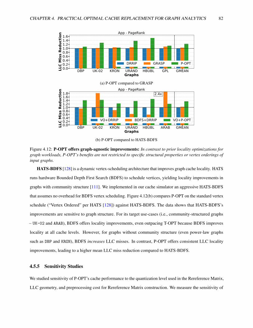
CHAPTER 4. PRACTICAL OPTIMAL CACHE REPLACEMENT FOR GRAPH ANALYTICS 82
DBP UK-02 KRON URAND HBUBL GPL GMEANGraphs
0.00.20.40.60.81.01.21.41.6
LLC
Mis
s Re
duct
ion App - PageRank
DRRIP GRASP P-OPT
(a) P-OPT compared to GRASP
DBP UK-02 KRON URAND HBUBL ARAB GMEANGraphs
0.00.20.40.60.81.01.21.41.61.8
LLC
Mis
s Re
duct
ion
2.4xApp - PageRank
VO+DRRIP BDFS+DRRIP VO+P-OPT
(b) P-OPT compared to HATS-BDFS
Figure 4.12: P-OPT offers graph-agnostic improvements: In contrast to prior locality optimizations forgraph workloads, P-OPT’s benefits are not restricted to specific structural properties or vertex orderings ofinput graphs.
HATS-BDFS [128] is a dynamic vertex-scheduling architecture that improves graph cache locality. HATS
runs hardware Bounded Depth First Search (BDFS) to schedule vertices, yielding locality improvements in
graphs with community structure [111]. We implemented in our cache simulator an aggressive HATS-BDFS
that assumes no overhead for BDFS vertex scheduling. Figure 4.12(b) compares P-OPT on the standard vertex
schedule (“Vertex Ordered” per HATS [128]) against HATS-BDFS. The data shows that HATS-BDFS’s
improvements are sensitive to graph structure. For its target use-cases (i.e., community-structured graphs
– UK-02 and ARAB), BDFS offers locality improvements, even outpacing T-OPT because BDFS improves
locality at all cache levels. However, for graphs without community structure (even power-law graphs
such as DBP and KRON), BDFS increases LLC misses. In contrast, P-OPT offers consistent LLC locality
improvements, leading to a higher mean LLC miss reduction compared to HATS-BDFS.
4.5.5 Sensitivity Studies
We studied sensitivity of P-OPT’s cache performance to the quantization level used in the Rereference Matrix,
LLC geometry, and preprocessing cost for Rereference Matrix construction. We measure the sensitivity of
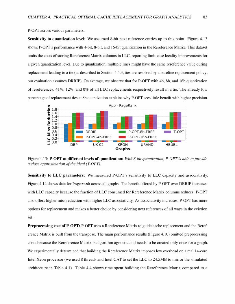
CHAPTER 4. PRACTICAL OPTIMAL CACHE REPLACEMENT FOR GRAPH ANALYTICS 83
P-OPT across various parameters.
Sensitivity to quantization level: We assumed 8-bit next reference entries up to this point. Figure 4.13
shows P-OPT’s performance with 4-bit, 8-bit, and 16-bit quantization in the Rereference Matrix. This dataset
omits the costs of storing Rereference Matrix columns in LLC, reporting limit-case locality improvements for
a given quantization level. Due to quantization, multiple lines might have the same rereference value during
replacement leading to a tie (as described in Section 4.4.3, ties are resolved by a baseline replacement policy;
our evaluation assumes DRRIP). On average, we observe that for P-OPT with 4b, 8b, and 16b quantization
of rereferences, 41%, 12%, and 0% of all LLC replacements respectively result in a tie. The already low
percentage of replacement ties at 8b quantization explains why P-OPT sees little benefit with higher precision.
DBP UK-02 KRON URAND HBUBLGraphs
0.00.20.40.60.81.01.21.41.61.8
LLC
Mis
s Re
duct
ion App - PageRank
DRRIPP-OPT-4b-FREE
P-OPT-8b-FREEP-OPT-16b-FREE
T-OPT
Figure 4.13: P-OPT at different levels of quantization: With 8-bit quantization, P-OPT is able to providea close approximation of the ideal (T-OPT).
Sensitivity to LLC parameters: We measured P-OPT’s sensitivity to LLC capacity and associativity.
Figure 4.14 shows data for Pagerank across all graphs. The benefit offered by P-OPT over DRRIP increases
with LLC capacity because the fraction of LLC consumed for Rereference Matrix columns reduces. P-OPT
also offers higher miss reduction with higher LLC associativity. As associativity increases, P-OPT has more
options for replacement and makes a better choice by considering next references of all ways in the eviction
set.
Preprocessing cost of P-OPT: P-OPT uses a Rereference Matrix to guide cache replacement and the Reref-
erence Matrix is built from the transpose. The main performance results (Figure 4.10) omitted preprocessing
costs because the Rereference Matrix is algorithm agnostic and needs to be created only once for a graph.
We experimentally determined that building the Rereference Matrix imposes low overhead on a real 14-core
Intel Xeon processor (we used 8 threads and Intel CAT to set the LLC to 24.5MB to mirror the simulated
architecture in Table 4.1). Table 4.4 shows time spent building the Rereference Matrix compared to a

CHAPTER 4. PRACTICAL OPTIMAL CACHE REPLACEMENT FOR GRAPH ANALYTICS 84
8MB 16MB 24MB 32MBLLC sizes
0.00.20.40.60.81.01.21.4
LLC
Mis
s Re
d.
App - PageRank
DRRIPP-OPT
12ways 16ways 20ways 24waysLLC ways
0.00.20.40.60.81.01.21.41.6
LLC
Mis
s Re
d.
App - PageRank
DRRIPP-OPT
Figure 4.14: Sensitivity to LLC size and associativity: P-OPT’s effectiveness increases with LLC size andassociativity.
baseline execution of Pagerank. On average, constructing the Rereference Matrix accounts for 19.8% of
Pagerank runtime 6. Figure 4.10 shows that without the Rereference Matrix construction cost, P-OPT offers
a mean performance improvement of 36% over DRRIP 7 for Pagerank. Since the Rereference Matrix is
algorithm agnostic, the preprocessing cost of P-OPT can be easily amortized by reusing the Rereference
Matrix across multiple applications running on the same graph. However, even in scenarios where the
Rereference Matrix construction cost cannot be amortized (e.g., single-shot graph analytics), the relatively
small cost of constructing the Rereference Matrix allows P-OPT to provide a net speedup even after including
the preprocessing cost.
DBP UK-02 KRON URND HBUBLPOPT Preprocessing Time 0.99s 1.25s 1.59s 1.77s 0.92sPageRank Execution Time 8.83s 24.64s 4.84s 11.06s 0.89s
Table 4.4: Relative preprocessing cost for P-OPT
4.6 Related Work
We compared P-OPT to the most closely related works in Sections 4.1 and 4.5. We include additional
comparisons spanning three areas – cache replacement, irregular-data prefetching, and custom architectures
for graph processing.
Replacement Policies: Hawkeye and SHiP outperform many classes of replacement policies [84, 167]. One
such class of policies are policies like SDBP [97] and Leeway [61] that perform Dead-Block Prediction
(DBP) (i.e. find cache lines that will receive no further accesses). P-OPT can more accurately identify
6HBUBL is an exception because Pagerank converges unusually quickly (3 iterations)7Server-class processors have been shown to use a variant of DRRIP [166]

CHAPTER 4. PRACTICAL OPTIMAL CACHE REPLACEMENT FOR GRAPH ANALYTICS 85
dead lines because it tracks next references of irregular lines (Indeed, P-OPT outperforms Hawkeye and
GRASP which were shown to be better than SDBP and Leeway respectively). By using close approximation
of precise next references (Section 4.5.5), P-OPT is expected to outperform heuristic-based reuse distance
predictions [55, 96].
Irregular Data Prefetching: IMP [169], HATS-VO [128], and DROPLET [25] are recent prefetchers
that were designed primarily to handle irregular accesses in graph processing and sparse linear algebra
applications. All three schemes are effective at reducing latency of irregular accesses but not necessarily
memory traffic. P-OPT reduces memory traffic through better LLC locality, making better use of the available
DRAM bandwidth. We note that next references in a graph’s transpose could also be used for timely
prefetching of irregular data. We leave the exploration of new prefetching mechanisms derived from the
Rereference Matrix and the interplay of P-OPT with hardware-based [10,25,128,169] or software-based [11]
irregular prefetching for future work.
Custom architectures for graph processing: Minnow [171] is an architecture for efficient worklist manage-
ment and optimizes worklist-based graph applications [145]. OMEGA [9] is a scratchpad-based architecture
for graph processing on power-law input graphs. Custom accelerators [75, 139] have been proposed that
optimize graph framework operations to accelerate common sub-computations across all applications using
the framework. P-OPT observes the pervasiveness of poor cache locality in graph applications and leverages
the readily-available transpose to guide better cache replacement. SpArch [179], an SpGeMM accelerator,
proposed dedicated hardware to run ahead (up to a fixed depth) and compute next references for irregular
data. P-OPT also uses next references for better replacement but relies on the transpose to more efficiently
access next references.
4.7 Discussion
Belady’s optimal cache replacement policy is considered an impractical replacement policy in most cases
because it relies on oracular knowledge of future accesses. The key insight presented in this chapter is that a
graph’s transpose encodes the next reference information for all vertices at all points of a graph application’s
execution, essentially serving as the oracle for optimal cache replacement (Section 4.2). The second major
insight present in this chapter is that, for the purposes of optimal cache replacement, we do not need precise
next reference information. A quantized version of the transpose (Rereference Matrix) contains sufficient

CHAPTER 4. PRACTICAL OPTIMAL CACHE REPLACEMENT FOR GRAPH ANALYTICS 86
information for P-OPT to provide significant cache miss reductions even after including the overheads of
accessing the replacement metadata (i.e. quantized next references). Since the Rereference Matrix is just
a quantized representation of the information in a graph’s transpose, constructing the Rereference Matrix
from the transpose incurs low overhead (Table 4.4). Therefore, P-OPT readily applies to graph analytics
workloads which already store both the CSR and CSC representations (Section 1.4.2). For the same reason,
P-OPT should also easily generalize to sparse linear algebra kernels where the input matrices are stored in
the CSR and CSC formats.
In conclusion, P-OPT leverages the information present within the commonly used CSR and CSC repre-
sentations to make near-optimal cache replacement decisions. Consequently, P-OPT is able to significantly
improve cache locality compared the heuristics-based state-of-the-art cache replacement policies.

Chapter 5
Generalizing Beyond Graph Analytics with
HARP
In the previous chapter, we saw that by leveraging the common graph representation (CSR and CSC), P-OPT
was able to improve cache locality across a range of graph applications on a diverse set of input graphs.
However, P-OPT’s benefits are restricted to graph analytics workloads (and other applications were inputs
are represented using CSR and CSC). It is desirable to have a more general cache locality optimization
since irregular memory accesses affect many applications beyond graph analytics. Propagation Blocking
is one such optimization. While Propagation Blocking was designed as a software-based cache locality
optimization for graph analytics and sparse matrix vector multiplication [28, 37], we show that Propagation
Blocking generalizes beyond graph analytics [19]. In this chapter, we show that Propagation Blocking
only requires that an application perform irregular updates and exhibit unordered parallelism (these two
properties cover a broad range of applications). Due to Propagation Blocking’s versatility, we focused on
identifying the inefficiencies of a Propagation Blocking execution on conventional multicore processors and
proposed architecture support to further improve the performance gains offered by Propagation Blocking.
Our proposed architecture, HARP, optimizes the Propagation Blocking execution of a range of applications
with irregular memory updates, offering speedups of up to 3.78x compared to Propagation Blocking. Like
P-OPT (Chapter 4), HARP’s locality improvements are agnostic to the input graph. However, unlike P-OPT,
HARP does not make any assumptions about the input representation which allows HARP to generalize to
many irregular applications beyond just graph analytics.
87

CHAPTER 5. GENERALIZING BEYOND GRAPH ANALYTICS WITH HARP 88
5.1 Pervasiveness of Irregular Memory Updates
Irregular memory access patterns are not unique to graph analytics workloads. Many applications perform
irregular memory updates which causes these applications to make sub-optimal use of the on-chip cache
hierarchy. In this section, we identify the common sources of irregular memory updates and characterize the
poor cache locality resulting from such irregular updates.
5.1.1 Sources of Irregularity
A common source of irregular memory accesses is the input data representation used by an application. Graph
analytics and sparse linear algebra applications often analyze inputs that are extremely sparse (a typical
adjacency matrix is > 99% sparse [50]). Therefore, compressed formats are essential for storing the input
graph/matrix in memory efficiently (Figure 5.1). The popular Compressed Sparse Row (CSR) format offers
the additional benefit of quickly identifying a vertex’s neighbors. As shown in Figure 5.1, the CSR uses
two arrays to represent outgoing edges (sorted by edge source IDs). The Neighbor Array (NA) contiguously
stores each vertex’s neighbors and the Offsets Array (OA) stores the starting offset of each vertex’s neighbor
list in the NA. While the CSR (and its transpose CSC) are a memory efficient representations allowing quick
access to vertex neighbors, they can lead to irregular memory accesses. The contents of the CSR/CSC are
arbitrarily ordered (contents of the NA in Figure 5.1) and are defined by the sparsity pattern and vertex
ordering of the input. Therefore, applications traversing the CSR/CSC and accessing a second data structure
based on the indices in the NA would perform irregular memory accesses. Besides data representations, other
input properties such as the distribution of keys for counting sort [45] can also contribute to irregular memory
accesses.
01
2
34
0
2 4 3 1
5 6
3
8 8
0 0
OA
NA
0
1 2
2 3
0
4 6
0
OA
NA 2 0 0
COO(EdgeList)
CSC(Incoming-neighbors)
CSR(Outgoing-neighbors)
0 12 01 00 22 30 40 3
Figure 5.1: Popular Compressed Representations

CHAPTER 5. GENERALIZING BEYOND GRAPH ANALYTICS WITH HARP 89
5.1.2 Poor Locality of Irregular Updates
Applications with irregular memory updates suffer from poor cache locality. Conventional cache hierarchies
are designed to optimize for spatial and temporal locality both of which are absent in irregular memory
access patterns. Using hardware performance counters, we characterized the Last Level Cache (LLC) miss
rates of applications performing irregular memory updates (methodology listed in Section 5.5.1). Figure 5.2
shows that a broad range of applications spanning graph analytics, graph pre-processing, integer sorting,
and sparse linear algebra suffer from poor LLC locality because of irregular updates. Prior graph analytics
characterization studies [25, 176] have shown that the implication of high LLC miss rates is that graph
applications can spend up to 80% of their execution time stalled on DRAM. The high LLC miss rates
resulting from irregular updates emphasizes the need for a cache locality optimization to improve the
performance of these applications.
PAGE-RANK
MULTI-BFS
DEG-CNT
NGH-POP*
COUNT-SORT*
SPMV TRANSPOSE* PINV* SYMPERM*
Applications
0%20%40%60%80%
100%
GraphAnalytics
Pre-Processing
Sparse LinearAlgebra
LLC Miss Rate (%)COMMUTATIVE UPDATES NON-COMMUTATIVE UPDATES
Figure 5.2: Locality of irregular updates: Applications with irregular updates experience a high LLC missrate.
5.2 Versatility of Propagation Blocking
Propagation Blocking (PB) has been shown to be an effective optimization for graph analytics work-
loads [28, 100]. We show that PB applies more broadly to any application exhibiting unordered parallelism
and, therefore, PB generalizes to applications beyond graph analytics. Unfortunately, software PB incurs
fundamental overheads that prevent achieving optimal performance. We conclude this section by identifying
the opportunity to improve PB’s benefits with architecture support.

CHAPTER 5. GENERALIZING BEYOND GRAPH ANALYTICS WITH HARP 90
5.2.1 High level Overview of Propagation Blocking
Propagation Blocking (PB) was originally developed to optimize Pagerank [28]. Figure 5.3 shows an
unoptimized Pagerank execution operating on a CSR input graph. The Pagerank execution streams in
edges and auxiliary data (auxData), and updates the vtxData array at dstk using the value auxData[srck].
The stream of indices (dstk) in the CSR are unordered and span the full range of the graph’s vertex IDs
(Figure 5.1). Therefore, an unoptimized SpMV execution suffers from poor cache locality because the
irregular update’s working set exceeds on-chip cache capacity.
PB improves cache locality of Pagerank by breaking the execution into two phases: Binning and
Accumulate. During Binning, a core streams in edges and auxiliary data but the core does not directly update
vtxData elements. Instead, the core writes the pair of index location and update value (dstk,auxData[srck])
to one of several bins created by PB. A bin is a data structure that sequentially stores each update belonging to
a particular range of data elements. Each bin stores updates for a disjoint range of elements and the union of
all the bin-ranges equals the total number of elements (i.e. number of vertices in the graph). Once all updates
have been written to bins, PB starts the Accumulate phase. During Accumulate, the core sequentially accesses
each tuple in a bin before moving to the next bin (Figure 5.3). Since each bin stores updates for a small
index range, only a part of the vtxData array is accessed at any point in time which reduces the range of
random writes, allowing the bin’s updates to fit in cache. In this work, we focus on parallel PB which simply
creates per-thread duplicates of all bin structures in Figure 5.3, eliminating the need for synchronization
during Binning.
5.2.2 Applicability of Propagation Blocking
The effectiveness of PB across many graph workloads [28, 37, 100] has prompted hardware optimizations for
PB [90,130,148]. However, these hardware PB optimizations rely on the application performing commutative
updates (i.e. the order of applying updates does not affect the final result). Commutative updates allow
coalescing multiple updates destined to the same index, reducing PB’s main memory traffic without affecting
application correctness.However, we find that commutativity is not necessary to benefit from PB.
We observe that PB applies to non-commutative kernels as well. Algorithm 6 shows a part of the kernel for
building a CSR from an Edgelist 1. The kernel (henceforth referred to as Neighbor-Populate) uses a copy
1Building a graph data structure from an Edgelist representation is one of three kernels used by Graph500 [133] to benchmarksupercomputers based on their graph processing capabilities.

CHAPTER 5. GENERALIZING BEYOND GRAPH ANALYTICS WITH HARP 91
auxData[src1]
dst2 auxData[src2]
dst1
Range of Random Accesses = |V|
Unoptimized Execution PB (Phase 1) -- Binning
UpdateList
Update List
binID = dstk / BinRange
CoalescingBuffers
Bins
. . .
. . .
. . .
. . .
for src in G: for dst in G.out_neigh(src): vtxData[dst] += auxData[src]
vtxData[dst1] += auxData[src1]
CSR auxData
BinRange = G.nodes / |bins| for src in G: for dst in G.out_neigh(src): binID = dst / BinRange bins[binID].append(dst, auxData[src])
for bin in bins: for tuple in bin: (dst, val) = tuple vtxData[dst] += val
vtxData[dstk] += Vk
Range = |BinRange|
Bins
PB (Phase 2) -- Accumulate
(dstk, Vk) Tuple
Core
Core
Core
Figure 5.3: High level overview of Propagation Blocking (PB): PB reduces the range of irregular updates.Note that the Update List exists only at a logical level and is never physically materialized.
Algorithm 6 Kernel to populate neighbors (Edgelist-to-CSR)
1: offsets← PrefixSum(degrees) . Offsets Array (OA) in Figure 5.12: par_for e in EL do3: neighs[offsets[e.src]]← e.dst . Neighbors Array (NA) in Figure 5.14: AtomicAdd(offsets[e.src],1)
Algorithm 7 PB version of Algorithm 6
1: offsets← PrefixSum(degrees)2: par_for e in EL do . Binning Phase3: tid← GetThreadID()4: binID← (e.src/BinRange)5: bins[tid][binID]← (e.src,e.dst)
6: par_for binID in NumBins do . Accumulate Phase7: for tid in NumThreads do8: for tuple in bins[tid][binID] do9: offsetVal← offsets[tuple.src]
10: neighs[offsetVal]← tuple.dst11: Add(offsets[tuple.src],1)
of the Offsets Array (OA) to populate the contents of the Neighbors Array (NA) in Figure 1.2. The updates to
the offsets array in Neighbor-Populate (Algorithm 6; line 4) are not commutative because the order of
updates to the offsets array determines the contents of the NA. The updates are not commutative because
Neighbor-Populate uses the offsets array to populate the neighs array, and the order of updates to the
offsets array changes the results in the neighs array2. Algorithm 7 shows how PB optimizes the kernel.
2Commutativity optimizations that coalesce updates to the offsets array elements would break correctness by skippingelements of the NA.

CHAPTER 5. GENERALIZING BEYOND GRAPH ANALYTICS WITH HARP 92
The Binning phase streams in edges and assigns each edge to a bin. After Binning reorganizes edges into
bins, Accumulate processes the edges in each bin, updating offsets and neighs with high cache locality.
The PB optimization is applicable to the non-commutative Neighbor-Populate kernel because a vertex’s
neighbors can be listed in any order; the non-commutative updates permit unordered parallelism [82, 88].
This example shows that the applicability of PB goes beyond commutative updates: the PB optimization
applies to applications with irregular updates and unordered parallelism. All the applications listed in
Figure 5.2 can benefit from PB however not all applications perform commutative updates and, therefore,
cannot benefit from existing hardware PB optimizations. The focus of our work is to develop a general
hardware PB optimization that does not rely on update commutativity, enabling acceleration of a broader
range of applications.
5.2.3 Limitations of Propagation Blocking
The performance of all PB executions on conventional multicore processors is primarily limited in two
ways: (i) PB must compromise by selecting a sub-optimal number of bins and (ii) binning updates requires
executing many additional instructions, which erode PB’s gains.
Compromising on the number of bins: The locality of the Accumulate phase (Figure 5.3) is highly
sensitive to the number of bins because the range of updates belonging to a bin (i.e. range of irregular updates)
is inversely related to the number of bins (BinRange = |UniqueIndices||Bins| ). The Binning phase is also sensitive to
the number of bins. To amortize the cost of writing to bins, the Binning phase uses cacheline-sized coalescing
buffers for each bin that accumulate updates to bins and enable coarse granularity writes to bins. Figure 5.4
shows the performance and cache locality of the Binning and Accumulate phases as the number of bins vary,
for the Neighbor-Populate kernel. The data in Figure 5.4b show normalized L1 load misses (broken into
L2, LLC, and DRAM accesses) collected using hardware performance counters (Section 5.5.1). Optimal
Accumulate performance is achieved when there are a large number of bins because the range of locations
modified by a bin’s updates is reduced to the point that they can fit within the L1 cache. However, selecting a
large number of bins is not feasible because the Binning phase achieves the worst performance as all the bins’
coalescing buffers do not fit in the L1 and L2 caches (Figure 5.4b). Competing requirements on the bin range
by Binning and Accumulate forces all PB execution to make a compromise and select a medium number of
bins (red dotted line in Figure 5.4a), leading to sub-optimal performance in both phases. The architecture

CHAPTER 5. GENERALIZING BEYOND GRAPH ANALYTICS WITH HARP 93
mechanism that we design in Section 5.3.2 shows how to break PB’s dependence on the number of bins and
get high performance in both phases without a compromise.
256 512 1K 2K 4K 8K 16K 32KNo. of Bins
0.00.51.01.52.02.53.03.54.04.5
Norm
alize
d Ti
me
BINNING
PB-SWPB-SW-IDEAL
256 512 1K 2K 4K 8K 16K 32KNo. of Bins
0.0
0.2
0.4
0.6
0.8
1.0
Norm
alize
d Ti
me
ACCUMULATEPB-SWPB-SW-IDEAL
(a) Execution time versus bin range
256 512 1K 2K 4K 8K 16K 32KNo. of Bins
0
20
40
60
80
100
Norm
. L1
Cach
e M
isses BINNING
L2LLCDRAM
256 512 1K 2K 4K 8K 16K 32KNo. of Bins
0.00.20.40.60.81.0
Norm
. L1
Cach
e M
isses ACCUMULATE
L2LLCDRAM
(b) Cache locality versus bin range
Figure 5.4: Sensitivity of PB to the number of bins: The Binning phase achieves better locality with fewerbins whereas the Accumulate phase prefers a large number of bin.
An ideal PB mechanism would use the best bin range for each phase – a large bin range for Binning and a
small bin range for Accumulate (green dotted lines in Figure 5.4a). Figure 5.5 shows PB’s performance gains
compared to this idealized version of PB. While this ideal PB variant is unrealizable, the data show ample
headroom for improvement. Using the optimal bin range in each phase, PB’s performance can improve by up
to 1.8x, amplifying its best case benefit over the unoptimized case to 8x.
DBP PLD KRON URAND EUROGraphs
0.01.02.03.04.05.06.07.08.0
Spee
dup
App - NeighPopulate
BASE PB-SW PB-SW-IDEAL
Figure 5.5: Ideal performance with Propagation Blocking: Allowing each phase to operate with the bestnumber of bins shows the headroom for performance improvement in PB.
Control overheads of Software PB: PB implemented in software requires executing extra instructions for
binning which degrades instruction level parallelism (ILP) by occupying core resources (e.g., reservation
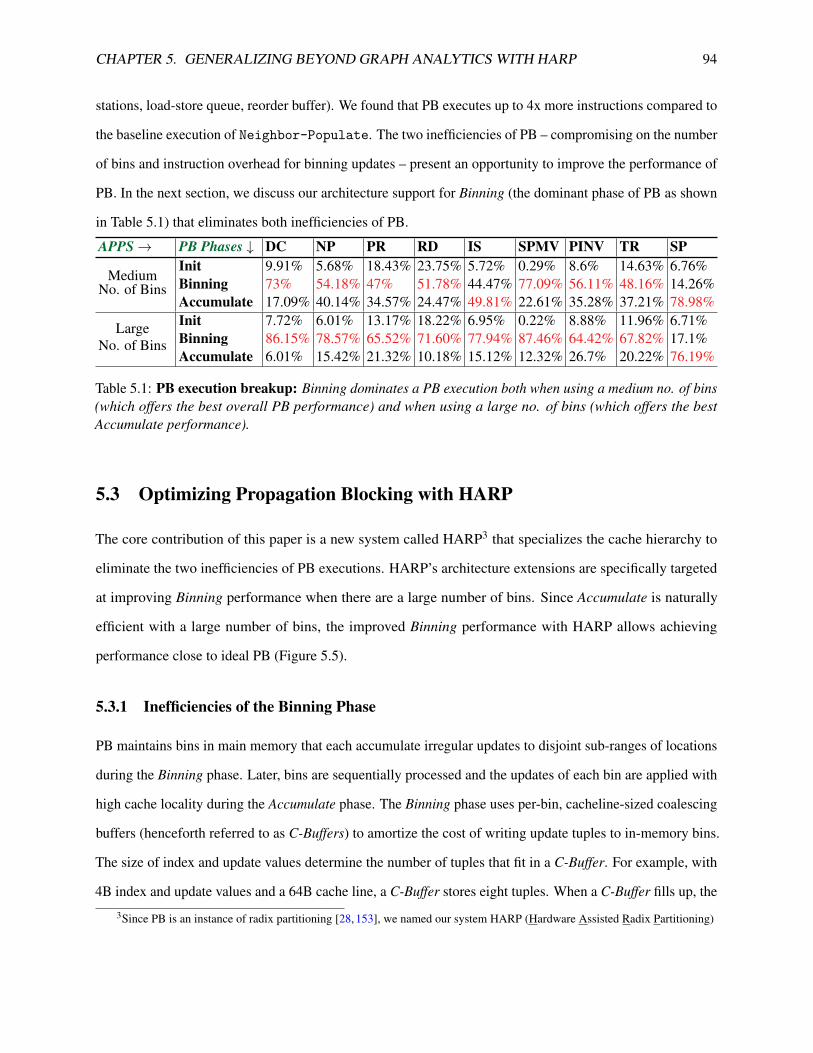
CHAPTER 5. GENERALIZING BEYOND GRAPH ANALYTICS WITH HARP 94
stations, load-store queue, reorder buffer). We found that PB executes up to 4x more instructions compared to
the baseline execution of Neighbor-Populate. The two inefficiencies of PB – compromising on the number
of bins and instruction overhead for binning updates – present an opportunity to improve the performance of
PB. In the next section, we discuss our architecture support for Binning (the dominant phase of PB as shown
in Table 5.1) that eliminates both inefficiencies of PB.
APPS→ PB Phases ↓ DC NP PR RD IS SPMV PINV TR SP
MediumNo. of Bins
Init 9.91% 5.68% 18.43% 23.75% 5.72% 0.29% 8.6% 14.63% 6.76%Binning 73% 54.18% 47% 51.78% 44.47% 77.09% 56.11% 48.16% 14.26%Accumulate 17.09% 40.14% 34.57% 24.47% 49.81% 22.61% 35.28% 37.21% 78.98%
LargeNo. of Bins
Init 7.72% 6.01% 13.17% 18.22% 6.95% 0.22% 8.88% 11.96% 6.71%Binning 86.15% 78.57% 65.52% 71.60% 77.94% 87.46% 64.42% 67.82% 17.1%Accumulate 6.01% 15.42% 21.32% 10.18% 15.12% 12.32% 26.7% 20.22% 76.19%
Table 5.1: PB execution breakup: Binning dominates a PB execution both when using a medium no. of bins(which offers the best overall PB performance) and when using a large no. of bins (which offers the bestAccumulate performance).
5.3 Optimizing Propagation Blocking with HARP
The core contribution of this paper is a new system called HARP3 that specializes the cache hierarchy to
eliminate the two inefficiencies of PB executions. HARP’s architecture extensions are specifically targeted
at improving Binning performance when there are a large number of bins. Since Accumulate is naturally
efficient with a large number of bins, the improved Binning performance with HARP allows achieving
performance close to ideal PB (Figure 5.5).
5.3.1 Inefficiencies of the Binning Phase
PB maintains bins in main memory that each accumulate irregular updates to disjoint sub-ranges of locations
during the Binning phase. Later, bins are sequentially processed and the updates of each bin are applied with
high cache locality during the Accumulate phase. The Binning phase uses per-bin, cacheline-sized coalescing
buffers (henceforth referred to as C-Buffers) to amortize the cost of writing update tuples to in-memory bins.
The size of index and update values determine the number of tuples that fit in a C-Buffer. For example, with
4B index and update values and a 64B cache line, a C-Buffer stores eight tuples. When a C-Buffer fills up, the
3Since PB is an instance of radix partitioning [28, 153], we named our system HARP (Hardware Assisted Radix Partitioning)

CHAPTER 5. GENERALIZING BEYOND GRAPH ANALYTICS WITH HARP 95
core bulk-transfers all of the C-Buffer’s tuples into its corresponding bin in memory and clears the C-Buffer
to start collecting tuples again.
The Binning phase has two main sources of inefficiency. First, Binning suffers poor cache performance
when there are a large number of bins. Figure 5.6 shows why Binning performs poorly with many bins in a
typical 3-level cache hierarchy. With a large number of bins, all the per-bin C-Buffers do not fit in a small
cache (e.g., L1), increasing the average latency of inserting tuples into C-Buffers. Compounding the problem,
increased cache demands by other program data can displace C-Buffers to lower levels of cache (e.g., LLC),
further increasing access latency. The second main inefficiency in Binning is that C-Buffers are managed
entirely in software. Extra instructions need to be executed to write to C-Buffers, detect when a C-Buffer fills,
and bulk-transfer the C-Buffer’s tuples to in-memory bins.
Core
Update List
binID = Indexk / BinRange
L1 Cache
L2 Cache
LLC
DRAM Bins
Propagation Blocking
SW Coalescing BuffersOther Data Cachelines
HARP
Update List
L1bufID = Indexk / L1BinRange
X C-
buffe
rs a
cros
s 3
leve
ls
L2bufID = Indexm / L2BinRange
LLCbufID = Indexn / LLCBinRange
Y3 >> X HW Coalescing Buffers
Y1 L1 C-Buffers
Y2 L2 C-Buffers
Y3 LLC C-Buffers
L1BinRange(RL1)
L2BinRange(RL2)
LLCBinRange(RLLC)
Core
Other Data Cachelines
Y3 > Y2 > Y1
RLLC < RL2 < RL1
Figure 5.6: Comparing Binning phases of PB and HARP: HARP maintains a hierarchy of HW-managedC-Buffers to provide the illusion of a small number of bins for Binning while actually using a large numberof bins for Accumulate. We do not show bins in DRAM for HARP (HARP uses Y3 bins in DRAM). The ratioof per-level bin ranges (RL1,RL2,RLLC) in HARP are defined by the input range and cache sizes.
CHAPTER 5. GENERALIZING BEYOND GRAPH ANALYTICS WITH HARP 96
5.3.2 An Architecture for Binning
HARP optimizes PB by enabling the selection of a large number of bins that offers optimal Accumulate
performance (Figure 5.4a) and changing the operation of the memory hierarchy to make Binning more
efficient with many bins. The key insight of HARP is to decouple Binning performance from the number of
bins in memory. Instead of using a single set of software-managed C-Buffers that can spread across the cache
hierarchy, HARP introduces a hierarchy of hardware-managed C-Buffers. Each level of the cache hierarchy
has its own set of C-Buffers with the number of C-Buffers in a level bounded by the capacity of that level.
Therefore, the L1 cache has the fewest C-Buffers and the Last Level Cache (LLC) has the most C-Buffers. In
contrast to software-PB where a single bin range maps update tuples to bins (Algorithm 7; Line 4), in HARP
each cache level has a unique bin range used to map tuples into one of the level’s C-Buffers. For example,
in Figure 5.6, the bin range used for mapping tuples into L1 C-Buffers is L1BinRange(RL1) =|UniqIndices|
|Y1|
while the bin range for the LLC is LLCBinRange(RLLC) =|UniqIndices|
|Y3| .
In HARP, a core interacts only with the L1 C-Buffers, writing tuples into one of the Y1 C-Buffers using by
the L1BinRange (L1Bu f f erID = IndexRL1
). When an L1 C-Buffer fills up, HARP does not transfer its contents
directly to an in-memory bin (as in software PB). Instead, HARP evicts the L1 C-Buffer by unpacking its
tuples and sending each tuple to its C-Buffer in the L2 cache. Unlike a traditional cache eviction where the
evicted line is sent to the next cache level as a whole, during an eviction each tuple in the filled C-Buffer in
level Li may need to be written to a different C-Buffer in the next cache level (Li+1). HARP writes each tuple
evicted from the filled L1 C-Buffer into one of Y2 C-Buffers in the L2 cache identified by the L2BinRange
(L2Bu f f erID = EvictedIndexRL2
). Similarly, when an L2 C-Buffer fills up, HARP evicts it from L2 and sends
each of its tuples to one of the Y3 C-Buffers present in the LLC. In HARP, the number of bins in memory
equals the number of LLC C-Buffers. Therefore, when finally a LLC C-Buffer fills up, HARP transfers all the
tuples in the filled LLC C-Buffer to the corresponding bin in main memory, as in a software-PB execution.
During the Binning phase in a HARP execution, all the tuples generated by the core are inserted into the L1
C-Buffers, eventually evicted into L2 C-Buffers followed by the LLC C-Buffers, before finally being written
to the bins in memory.
The hierarchical buffering mechanism in HARP causes each C-Buffer eviction to scatter tuples across
the C-Buffers of the next cache level. A small number of eviction buffers between cache levels suffice to
hide the latency of scattering tuples and remove C-Buffer eviction latency off the critical path (Section 5.4.4).

CHAPTER 5. GENERALIZING BEYOND GRAPH ANALYTICS WITH HARP 97
Consequently, for the example in Figure 5.6, during the Binning phase the core observes a latency of inserting
tuples into a small number of bins (Y1 C-Buffers at the L1) while actually operating on a large number of bins
in memory (equal to the Y3 C-Buffers at the LLC).
Besides hierarchical buffering, the HARP architecture offers a second major efficiency boost to Binning.
HARP relies on simple fixed function logic in each cache level’s controllers to handle C-Buffer management
operations (such as detecting when a C-Buffer fills, and unpacking tuples from a filled Li C-Buffer and
inserting each tuple to an appropriate Li+1 C-Buffer). HARP reserves space within each cache level to pin
C-Buffers for the entirety of Binning (Figure 5.6), allowing simple logic to determine the unique location of a
C-Buffer within a cache level. Offloading C-Buffer management to hardware allows HARP to eliminate the
additional instruction overhead of Binning in software-based PB.
5.4 Architecture Support for HARP
The HARP architecture extends a baseline multicore processor to optimize Binning and Accumulate phases
in parallel PB. HARP’s extensions include extensions to the cache controllers to manage Coalescing buffers
(C-Buffers), and a small amount of buffering to hide C-Buffer eviction latencies.
5.4.1 Caches Designed for Binning
HARP modifies the cache hierarchy in two ways. First, HARP uses widely available way-based cache
partitioning [7] to reserve space for C-Buffers within each cache level, ensuring that other program data never
displace C-Buffers. Second, HARP keeps a hierarchy of C-Buffers. Each level in the cache hierarchy has its
own set of C-Buffers bounded by the level’s capacity. HARP also uses a unique bin range for each cache
level to map update tuples into one of the level’s C-Buffers. Practically, a cache level’s bin range must also be
a power of two, which makes it cheap to bin a tuple (i.e., the division in line 4 of Algorithm 7 can be replaced
by a bitshift).
A new instruction – bininit – configures the number of ways to reserve for C-Buffers at each cache
level. The bininit instruction takes four operands: (1) a cache level identifier (e.g., L1, L2, or LLC in most
systems), (2) number of ways to reserve for C-Buffers, (3) number of unique indices in the data namespace
(e.g., the number of vertices in a graph), and (4) tuple size in bytes. A program executes bininit once for
each cache level. bininit first reserves the specified number of cache ways and then computes the smallest

CHAPTER 5. GENERALIZING BEYOND GRAPH ANALYTICS WITH HARP 98
power-of-two bin range for which C-Buffers fit in the reserved cache ways. This per-level bin range is stored
in a special register, used later during Binning. Due to the power-of-two requirement on bin ranges, the
C-Buffers may not use all the reserved ways. So the bininit instruction saves the number of ways actually
used by C-Buffers to allow other data to reclaim unused ways.
The number of ways to reserve at a cache level depends on the cache pressure from non-C-Buffer accesses.
For our simulated architecture, we reserve all but one way in each level of cache except the L2 cache. Due to
the presence of an L2 stream prefetcher, we reserve a single way for L2 C-Buffers to retain cache capacity
for prefetched data. Later, we show that HARP’s performance is not very sensitive to the number of ways
reserved for C-Buffers (Figure 5.13b).
5.4.2 An ISA Extension for Binning
HARP eliminates the overhead of extra instructions in PB by extending the ISA with a new instruction –
binupdate. The binupdate instruction replaces all Binning related operations performed in a baseline
software PB execution. The binupdate instruction takes two operands - an index and a value to be used to
update the data stored at the index. For example, the Binning phase in lines 3–5 of Algorithm 7 would be
replaced by a single instruction {binupdate e.src e.dst}. Dedicated hardware in the cache controller
identifies the right C-Buffer for the input tuple and inserts the tuple (e.src, e.dst) into that C-Buffer.
CBuf0
CBuf1
CBuf2
CBuf3
CBuf4
CBuf5
CBuf6
CBuf7
CBuf8
CBuf9
CBuf10
ReservedWays
BufIDbits log2(BinRange)
SetbitsWaybitslog2(numSets)
IndexID UpdateVal IncomingTuple
Figure 5.7: C-Buffer organization within each cache level: Each cache level has a unique bin range thatis used to map an incoming tuple into one of the C-Buffers pinned in cache.
To use HARP, a program first executes the bininit instruction for each cache level and then starts
binning data using binupdate instructions. A binupdate instruction uses the index part of its input tuple
to find a target L1 C-Buffer, as shown in Figure 5.7. Since the bin range is a power-of-two, the lower
log2(bin_range) bits of the index represent an intra-bin-range offset and the remaining bits identify the buffer
ID. Reserving ways allows each C-Buffer to have a unique location within the cache and, hence, the buffer

CHAPTER 5. GENERALIZING BEYOND GRAPH ANALYTICS WITH HARP 99
ID further breaks down into sets bits and way bits, fully determining the location of the C-Buffer within the
cache4.
5.4.3 Inserting tuples into C-Buffers
HARP collects update tuples in cacheline-sized C-Buffers. When a C-Buffer fills with update tuples, the cache
evicts the C-Buffer line, scattering its tuples into the C-Buffers of the next level of the memory hierarchy.
HARP adds fixed function logic at the cache controller to support inserting an update tuple into a C-Buffer.
Normally, a cache uses the address to identify the bytes to be accessed within a cache line. A binupdate
instruction accesses a cache line differently, because the C-Buffer that the line contains is not byte addressable.
To insert a tuple into a C-Buffer, HARP must determine the tuple’s offset within the C-Buffer line. HARP
maintains offset counters for each C-Buffer to explicitly track the offset of the next tuple within each C-Buffer
line, essentially providing append-only access to C-Buffer lines. To insert a tuple into a C-Buffer, the
controller first reads the offset counter, inserts the tuple at the right offset within the C-Buffer line, and
increments the counter to point to the location for the next incoming tuple. When a C-Buffer cache line fills,
the counter wraps around to zero.
For storing per-C-Buffer offset counters, HARP repurposes existing metadata bits associated with the
cache lines containing C-Buffers. Repurposing these bits is safe because a C-Buffer line exists outside
the shared-memory address space (i.e. C-Buffers only reside in the cache hierarchy and are not present in
memory). HARP can also repurpose the coherence state bits because C-Buffers are core-private (software PB
already duplicates all bins and C-Buffers across threads as shown in Algorithm 7). As an example, a typical
tuple size of 8B (4B for index and value) requires tracking 8 tuples in a typical 64B cache line. For tracking
the 8 tuples within L1 and L2 cache lines, HARP can repurpose 1bit from PLRU replacement, 1bit from dirty
status bit, and 2bits from the MESI coherence status bits for a 3-bit offset counter.
5.4.4 Handling C-Buffer evictions
As the binupdate instruction fills L1 C-Buffers with tuples, eventually a L1 C-Buffer fills and HARP must
evict its tuples to C-Buffers in the next cache level (L2). When a C-Buffer fills up, HARP is responsible for
inserting each tuple in the full butter into the appropriate C-Buffer in the next cache level. After an eviction,
the C-Buffer is empty and can service future incoming tuples.4For non power-of-two sets (which is atypical), Set = (Bu f ID)%(numSets) and Way = Bu f ID/numSets.

CHAPTER 5. GENERALIZING BEYOND GRAPH ANALYTICS WITH HARP 100
LiCacheEvictionBuffer
Ctr...
C-BufferFull
Li+1 CacheCachelinetoTuples
T0
T0-Tk...
BinningEngine
T1 T2 Tk
Figure 5.8: Handling evictions when a C-Buffer fills up: Eviction buffers hide the latency of evictingtuples.
In a naive implementation, the filled C-Buffer line is evicted and directly sent to a dedicated hardware
unit within the cache controller called the binning engine. The binning engine sequentially extracts tuples
from an evicted C-Buffer cache line and serially issues each tuple to the C-Buffers in the next level of cache.
The process of inserting a tuple into the next cache level’s C-Buffer is exactly the same as a binupdate
instruction inserting tuples into an L1 C-Buffer (Figure 5.7). HARP inserts each evicted tuple into a C-Buffer
in the next cache level using that level’s unique bin range. Figure 5.8 shows how HARP evicts a full C-Buffer.
The cache controller determines when to evict a C-Buffer cache line by monitoring the line’s offset counter,
which is incremented on each tuple insertion. When the counter wraps around, the C-Buffer line is at capacity
and HARP evicts the line.
In the above naive implementation, HARP incurs the full eviction latency to sequentially issue all tuples
from a filled buffer to the C-Buffers in the next level of cache. To hide the latency of C-Buffer evictions,
HARP uses a set of first-in/first-out (FIFO) eviction buffers between cache levels. When a C-Buffer fills,
HARP simply inserts the cache line containing all of its tuples into the eviction buffer. Later, the binning
engine pulls a C-Buffer line from the eviction buffer, extracts tuples from the line, and inserts the tuples
into next level’s C-Buffers. Accounting for the eviction rate from each level of cache and the cycle time to
serially insert all the tuples to the next level of cache, Little’s Law [83] suggests that a 14-entry eviction
buffer between L1 and L2 and single entry eviction buffer between L2 and LLC hides all eviction latency.
However, Little’s law assumes steady state eviction rate and does not account for bursts in evictions, which
may underestimate the eviction buffer size. In a later section, we refine the Little’s Law estimate using a DES
model that accounts for bursts and the model shows that a 32-entry eviction buffer between L1 and L2 fully
hides C-Buffer eviction latency (Figure 5.13a) .

CHAPTER 5. GENERALIZING BEYOND GRAPH ANALYTICS WITH HARP 101
5.4.5 Additional implementation details
HARP manages the LLC differently from L1 and L2 because the LLC is shared among all the cores and
evictions of LLC C-Buffers interact with bins in main memory.
C-Buffers organization in NUCA caches: As Section 5.2.2 explains, PB creates a per-thread duplicate of
bins and C-Buffers and HARP exploits the duplication by making the C-Buffer in each level private to a core.
For core-private caches, most cache space is reserved for the C-Buffers. In a shared, NUCA LLC that is
physically distributed across cores, HARP evenly divides NUCA cache banks among cores. Each cores’ LLC
C-Buffers use the set of NUCA banks assigned to that core only. Our simulated architecture (Section 5.5.1)
models a typical three-level cache hierarchy where the L1 and L2 caches are core-private and the LLC is a
NUCA cache with a bank associated with each core. For this cache hierarchy, the number of LLC C-Buffers
for each core is bounded by the capacity of the core-local NUCA bank.
Evicting from LLC: Eviction of a full LLC C-Buffer moves buffered updates to a bin in memory, which is
unlike a C-Buffer eviction to the next cache level (Section 5.4.4). The process of evicting a C-Buffer from
the LLC depends on how HARP represents bins in memory. HARP assumes threads’ bin data are stored
sequentially in memory, as in Figure 5.9: for each thread, tuples belonging to a bin are stored contiguously.
Sequential, in-memory bin organization requires pre-computing the number of tuples in each bin (for each
thread). Fortunately, a baseline PB execution already counts tuples per bin (encoded in the BinO f f set array)
as a preprocessing step (Init phase in Table 5.1) to avoid dynamic memory allocation overheads during
Binning. With the above organization, each core can store the base pointer for its thread’s bin data structures
and use per-bin offsets to access each bin. When an LLC C-Buffer fills up, HARP writes the buffered tuples
to the bin data structure at the location pointed by BinO f f set[binID]. After an eviction from LLC, the bin
offset is incremented by the number of tuples in the C-Buffer.
Bin0 Bin1 Bin2 ...
BinBasePtr BinOffset[1]
T0 T1 TkBinOffset TupleCtr
LLCC-BufferCacheline
64B CachelineTagbits ReplacementMetadatabits
LLCprogramdataCacheline
BinOffset[2] BinOffset[3]
Bin3
. . .
BinDataStructure
Figure 5.9: Organization of per-thread bins in memory: BinOffsets are stored in the tag bits of LLCC-Buffer cachelines.

CHAPTER 5. GENERALIZING BEYOND GRAPH ANALYTICS WITH HARP 102
Storing the bin offset pointer requires no additional storage. Since the LLC C-Buffers are designed to fit
in a core’s local NUCA bank, the tag bits for the C-Buffer cacheline are unnecessary and can be repurposed to
store bin offsets (BinO f f set[binID]) as shown in Figure 5.9. Before Binning, HARP initializes the starting
offsets for each LLC C-Buffer (in every NUCA bank) in the C-Buffer’s tag entry using a new ISA instruction
that takes a buffer ID and starting bin offset as operand. At a LLC C-Buffer eviction, the contents of the
LLC C-Buffer line are written to the memory address computed using the bin offset in line’s tag entry
(BinBasePtr+BinO f f set[binID]). To avoid the need for address translation, we assume system support for
ensuring matching virtual and physical addresses for important data structures (eg. the bin data structure) as
proposed in prior work [81, 130]. After writing the contents of the full LLC C-Buffer to an in-memory bin,
the bin offset value in the cacheline’s tag is incremented by the number of tuples in the C-Buffer using fixed
function logic and the C-Buffer’s offset counters are reset to starting receiving tuples again.
Flushing the Cache After Binning: In HARP, all tuples are inserted by a binupdate instruction into L1
C-Buffers, later evicted to L2 and LLC C-Buffers, and eventually written to a bin in main memory. When
Binning ends, some tuples may still be resident in a C-Buffer in cache. Before starting the next phase of PB
(Accumulate), HARP must ensure that all remaining tuples in cache end up in in-memory bins. We add a
binflush ISA instruction that signals the end of Binning and causes each cache level’s controller to serially
walk all C-Buffer cache lines, forcing an eviction if the line is non-empty. In each core, binflush starts
with L1, proceeds to L2 and, finishes by writing the residual tuples in the local NUCA bank to memory.
The eviction process initiated by binflush proceeds as described in Sections 5.4.4 and 5.4.5, with the
difference that the eviction buffers, binning engine, and bin offsets update logic must handle partially filled
C-Buffers. The number of tuples remaining in a C-Buffer are identified with the help of per-C-Buffer offset
counters (Figures 5.8,5.9). In addition to being used at the end of Binning, binflush is also invoked in case
a page containing per-thread bin data structures is swapped out of memory. Such premature invocations of
binflush can be avoided by locking critical pages in memory (e.g., using mlock() in Linux).
Handling virtualization: HARP extends a commodity multicore processor to accelerate PB, requiring
its extensions to support virtualization for OS preemption and context switching. We rely on per-process,
way-partitioning (as in Intel CAT [7]) to reserve space for per-level C-Buffers across the cache hierarchy.
Using static cache partitioning for the HARP process ensures that each level’s C-Buffers are pinned for the
duration of the Binning phase of PB. However, if the HARP process is preempted during Binning, then
other processes scheduled to run intermediately can evict C-Buffer cache lines. Evictions triggered by other

CHAPTER 5. GENERALIZING BEYOND GRAPH ANALYTICS WITH HARP 103
processes may lead to transfer of partially-filled C-Buffer cache lines which reduces the efficiency of data
transfer. Fortunately, HARP’s architecture extensions significantly optimize Binning phase latency, allowing
Binning to complete with the minimum number of OS preemptions. Later, we show that HARP’s Binning
phases is not sensitive to the OS scheduling quantum (Figure 5.13c)
Need for Static Cache Partitioning: The HARP architecture described to this point assumes static cache
partitioning at each cache level to reserve space for C-Buffers and ensure that that C-Buffer accesses never
miss. HARP can also work in architectures lacking support for static cache partitioning. However, without
static cache partitioning, locality of C-Buffer cache lines is defined by the underlying cache replacement
policy and pressure from other data accesses during the Binning phase. Fortunately, all other data accesses
besides C-Buffers are streaming accesses (e.g., CSR and auxData in Figure 5.3) and do not impose cache
pressure on C-Buffer cache lines. Evaluations using a custom cache simulator revealed that the baseline
replacement policy (PLRU in L1/L2 and DRRIP in LLC) is able to provide a C-Buffer miss rate of <1% in
the absence of static cache partitioning.
Hardware overheads of HARP: HARP repurposes cache line metadata whenever possible (Figure 5.9) and
the only storage overhead incurred by HARP are the eviction buffers used to hide C-Buffer eviction latency.
However, the small eviction buffers between cache levels amount for less than 7% of an L1 cache area [131].
Finally, the binning engine and fixed function logic to update per-C-Buffer counters incur low complexity
because they perform simple integer arithmetic.
5.5 Performance Improvements with HARP
HARP provides significant performance and locality improvements across a diverse set of applications. We
provide a detailed quantitative explanation for HARP’s speedups and compare HARP against a state-of-the-art
Propagation Blocking optimization [130]. Before presenting our performance results, we briefly describe our
evaluation setup.
5.5.1 Evaluation Setup
We evaluated HARP across applications spanning graph processing, pre-processing, integer sort, and sparse
linear algebra using an architecture simulator.

CHAPTER 5. GENERALIZING BEYOND GRAPH ANALYTICS WITH HARP 104
Real System: Experiments in Sections 5.1, 5.2, and 5.5.5 were run on an Intel Xeon processor (14 cores,
35MB LLC, 32GB DRAM) with hyperthreading and “turbo boost” DVFS disabled. We used LIKWID [162]
to collect performance counters.
Simulator: We use Sniper [38] to evaluate HARP. Table 5.2 shows the architecture parameters we
simulated, with cache timing parameters collected from CACTI [131]. We made several modifications to
Sniper. For PB, we added support for non-temporal stores which are required for efficient Binning [28, 153].
For HARP, we model the interaction of the binupdate instruction with the Out-of-Order engine. We ensure
that a binupdate only retires when it reaches the head of the ROB because a binupdate writes the data
caches (i.e., like a store). Since no instruction depends on binupdate, we do not need to add binupdate
to the store queue for memory disambiguation. Stores require two ports to issue (address generation and
data), but the binupdate does not need the address generation port because the L1 C-Buffers are directly
addressed based on operand value. We also use a custom Pin-based [119] cache simulator for a subset of our
evaluations (Section 5.5.4). The cache simulator models the cache hierarchy in Table 5.2 and we validated
our cache simulator against Sniper – LLC statistics from our simulator are within 5% of Sniper).
Cores 16 OoO-cores, 2.66GHz, 4-wide issue, 128-entry ROB, 48-entry Load Queue, 32-entry StoreQueue
L1(D/I) 32KB, 8-way set associative, Bit-PLRU policy, Load-to-use = 3 cyclesL2 256KB, 8-way set associative, Bit-PLRU policy, Load-to-use = 8 cyclesLLC 2MB/core, 16-way set associative, DRRIP replacement policy [86], Load-to-use = 21 cycles (local
NUCA bank)NoC 4x4 mesh, 2 cycles hop-latency, 64 bits/cycle link B/W, MESI coherenceDRAM 80ns access latency
Table 5.2: Simulation parameters
Workloads: We evaluate HARP across workloads spanning multiple domains. Degree-Counting
and Neighbor-Populate are the dominant phases of Edgelist-to-CSR conversion, an important graph
preprocessing step that prior work has shown can be as expensive as the downstream graph analytics
kernel [123, 149]. Pagerank is a popular graph analytics kernel representative of graph applications where
all vertices are processed every iteration. Our Edgelist-to-CSR conversion and Pagerank implementations
are from the GAP [27] benchmark suite. Radii from the Ligra [154] benchmark suite estimates a graph’s
diameter by performing multi-source BFS and is representative of graph applications which only process
a subset of the vertices every iteration. In addition to graph (pre)processing workloads, we also evaluate
Integer Sorting. We use __gnu_parallel::sort() as our baseline sort implementation because we

CHAPTER 5. GENERALIZING BEYOND GRAPH ANALYTICS WITH HARP 105
found it to be up to 14% faster (2.7% on average) compared NAS benchmark suite’s [15] integer sort
implementation. The PB and HARP versions optimize a parallel counting sort implementation [45]. We
also evaluate HARP across four sparse linear algebra kernels – SpMV from the HPCG benchmark [54], and
PINV, Transpose, and SymPerm from the SuiteSparse benchmark suite [49]. PINV computes the inverse
mapping for a given permutation of a matrix rows/columns. Transpose constructs the sparse representation
of a matrix’s transpose. SymPerm permutes the upper triangular portion of a matrix and is a subroutine in
Cholesky factorization. To reduce simulation time, we simulate a single iteration of Pagerank because of its
constant runtime across iterations and we use iteration sampling [128, 130] to simulate every second pull
iteration for Radii.
Our workloads have tuple sizes of 4B (Degree-Counting and Integer Sort), 8B (Neighbor-Populate,
Pagerank), and 16B for the rest. PB (and HARP) require an application to perform irregular update and
streaming reads which required slight modifications for Pagerank, Radii, and SpMV (specifically making
the propagation blocking versions process the transpose representation of the input graph/matrix). For the PB
runs, we use the original source code which we received from the authors [28] and we simulated multiple bin
ranges for PB, selecting the best bin range for each workload and input graph pair.
Inputs: We evaluate the graph (pre)processing workloads across a diverse set of input graphs (the graphs
cover power-law, uniform normal, and bounded degree distributions). For Integer Sort, we sort 256
million randomly generated keys with varying values of the maximum key value. We use sparse matrices
representative of simulation and optimization problems for evaluating the sparse linear algebra kernels. All
our inputs cause the working set size to far exceed the LLC capacity. We do not simulate Radii on the EURO
graph because Radii never executes a pull iteration.
GRAPHS DBP [103] PLD [112] KRON [27] URND [27] EURO [50]# Vertices 18.26M 42.89M 33.55M 33.55M 50.91M# Edges 136.54M 623.06M 133.52M 134.22M 108.11M
MATRICES HBUBL [50] HTRACE [50] KMER [50] DELAUNAY [50]# Rows/Columns 21.12M 16M 67.72 16.78M# NNZs 63.58 48M 138.78M 100.66M
Table 5.3: Input Graphs and Matrices

CHAPTER 5. GENERALIZING BEYOND GRAPH ANALYTICS WITH HARP 106
DBP PLD KRON URND EURO GMEANInputs
0.00.51.01.52.02.53.0
Spee
dup
DEGREE-COUNT (DC)
DBP PLD KRON URND EURO GMEANInputs
0.02.04.06.08.0
10.012.0
Spee
dup
NEIGHBOR-POPULATE (NP)*
DBP PLD KRON URND EURO GMEANInputs
0.00.51.01.52.0
Spee
dup
PAGERANK (PR)
DBP PLD KRON URND GMEANInputs
0.00.51.01.52.0
Spee
dup
RADII (RD)
225 226 227 GMEANKey Ranges
0.01.02.03.04.05.06.07.0
Spee
dup
INTEGER SORT (IS)*
HBUBL HTRACE KMER DELAUNAY GMEANInputs
0.00.51.01.52.02.53.03.54.04.5
Spee
dup
SPMV
HBUBL HTRACE KMER DELAUNAY GMEANInputs
0.00.51.01.52.0
Spee
dup
PINV*
HBUBL HTRACE KMER DELAUNAY GMEANInputs
0.02.04.06.08.0
10.012.0
Spee
dup
TRANSPOSE (TR)*
HBUBL HTRACE KMER DELAUNAY GMEANInputs
0.00.20.40.60.81.01.2
Spee
dup
SYMPERM (SP)*
BASEPB-SW
PB-SW-IDEALHARP
Figure 5.10: Speedups with HARP: HARP provides significant performance gains over PB-SW (and PB-SW-IDEAL) across a broad set of applications. (* indicates that the application performs non-commutativeupdates)
5.5.2 Speedups with HARP
The main result of this evaluation is that HARP consistently improves the performance of PB. HARP improves
PB performance in two ways – by eliminating the need to compromise with a sub-optimal number of bins
and by eliminating the instruction overheads associated with Binning. To isolate the contributions from each
optimization, Figure 5.10 compares speedups from a baseline software-based PB (PB-SW), PB-SW-Ideal
(an idealized PB execution combining Binning with a small number of bins and Accumulate with a large
number of bins), and HARP. PB is an effective software locality optimization offering a mean speedup of
1.81x over the baseline. Eliminating the compromise on the bin range parameter (PB-SW-IDEAL) provides
an additional mean speedup of 1.2x over PB. HARP combines the benefits of using the optimal number of
bins for Accumulate with the efficiency improvements from offloading C-Buffer management to hardware,
allowing HARP to gain an additional mean speedups of 1.45x over PB-SW-IDEAL. In summary, HARP
provides a mean speedups of 1.74x over PB and 3.16x over the baseline. These HARP speedup numbers
include the cost of initializing LLC C-Buffers tags with starting bin offset values and flushing every level’s
C-Buffers after Binning (Section 5.4.5). The numbers in Figure 5.10 also account for the initialization cost of
computing per-thread bin sizes in both HARP and PB. The results for PINV and SymPerm need additional
explanations. PINV was the only application where the best Accumulate performance did not correspond with
a large number of bins (likely due to parallelism artifacts overshadowing the locality benefits). Consequently,
PB-SW-IDEAL underperforms PB-SW for PINV and HARP offers limited benefits over PB-SW. We ran a
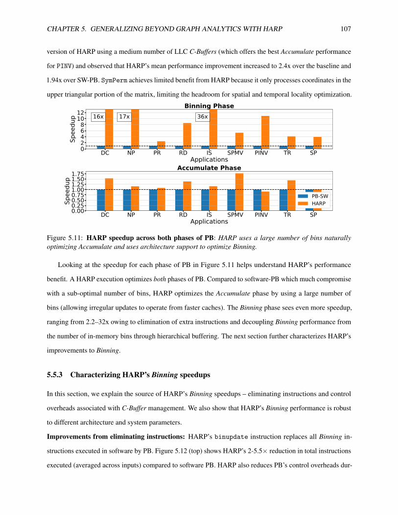
CHAPTER 5. GENERALIZING BEYOND GRAPH ANALYTICS WITH HARP 107
version of HARP using a medium number of LLC C-Buffers (which offers the best Accumulate performance
for PINV) and observed that HARP’s mean performance improvement increased to 2.4x over the baseline and
1.94x over SW-PB. SymPerm achieves limited benefit from HARP because it only processes coordinates in the
upper triangular portion of the matrix, limiting the headroom for spatial and temporal locality optimization.
DC NP PR RD IS SPMV PINV TR SPApplications
02468
1012
Spee
dup 16x 17x 36x
Binning Phase
DC NP PR RD IS SPMV PINV TR SPApplications
0.000.250.500.751.001.251.501.75
Spee
dup
Accumulate Phase
PB-SWHARP
Figure 5.11: HARP speedup across both phases of PB: HARP uses a large number of bins naturallyoptimizing Accumulate and uses architecture support to optimize Binning.
Looking at the speedup for each phase of PB in Figure 5.11 helps understand HARP’s performance
benefit. A HARP execution optimizes both phases of PB. Compared to software-PB which much compromise
with a sub-optimal number of bins, HARP optimizes the Accumulate phase by using a large number of
bins (allowing irregular updates to operate from faster caches). The Binning phase sees even more speedup,
ranging from 2.2–32x owing to elimination of extra instructions and decoupling Binning performance from
the number of in-memory bins through hierarchical buffering. The next section further characterizes HARP’s
improvements to Binning.
5.5.3 Characterizing HARP’s Binning speedups
In this section, we explain the source of HARP’s Binning speedups – eliminating instructions and control
overheads associated with C-Buffer management. We also show that HARP’s Binning performance is robust
to different architecture and system parameters.
Improvements from eliminating instructions: HARP’s binupdate instruction replaces all Binning in-
structions executed in software by PB. Figure 5.12 (top) shows HARP’s 2-5.5× reduction in total instructions
executed (averaged across inputs) compared to software PB. HARP also reduces PB’s control overheads dur-

CHAPTER 5. GENERALIZING BEYOND GRAPH ANALYTICS WITH HARP 108
DC NP PR RD IS SPMV PINV TR SP0.01.02.03.04.05.0
Reduction in Instructions
DC NP PR RD IS SPMV PINV TR SPApplications
0%5%
10%15%
Branch Misprediction Rate (%)PB-SW HARP
Figure 5.12: Efficiency gains from eliminating instruction overhead of binning: The binupdate instruc-tion in HARP enables an OoO core to exploit more ILP.
ing Binning. PB manages C-Buffers in software: after every tuple insertion the core must check if a C-Buffer
is full. HARP instead manages C-Buffers using dedicated hardware in the cache controller, reducing the rate
of branch mispredictions, as Figure 5.12 (bottom) shows. HARP eliminates all branch misses associated
with managing C-Buffers in software, often achieving near-zero branch misprediction rates as the baseline
versions5. By reducing the instruction and control overheads of Binning, HARP enables an Out-of-Order
processor to better exploit Instruction Level Parallelism (ILP) and we observe that the Instructions-per-Cycle
(IPC) of the Binning phase improves from 0.71 in PB-SW to 1.55 in HARP.
Sensitivity to eviction buffer sizes: HARP uses eviction buffers to push C-Buffer eviction latencies off
the critical path. We built a Discrete Event Simulation (DES) model of HARP to estimate the eviction
buffer sizes required to handle input-specific eviction bursts. The DES model consumes a trace of update
tuples and reports the fraction of time stalled on a full eviction buffer. Figure 5.13a reports the fraction of
Neighbor-Populate execution stalled for different sizes of eviction buffer between L1 and L2. The data
show that a 32-entry L1 eviction buffer hides eviction latency for all inputs. Little’s Law estimates that a
single-entry buffer between L2 and LLC suffices because L2 evictions are infrequent. Overprovisioning the
buffer to 8 entries incurs a modest cost and should suffice to handle rare bursts of L2 evictions [83].
Sensitivity to ways reserved for C-Buffers: HARP uses way partitioning to reserve space for C-Buffers at
each cache level, reducing the effective cache capacity for non-C-Buffer data during Binning. We measured
5Pagerank and Radii still incur branch misses because accessing a CSR, especially of power-law graphs, incurs controlinstructions to check if all the neighbors of a vertex have been processed. SymPerm incurs branch misses because it frequently needsto check if a non-zero coordinate belongs to the upper triangular matrix

CHAPTER 5. GENERALIZING BEYOND GRAPH ANALYTICS WITH HARP 109
2 4 8 16 32 64 128L1 buffer sizes
0%10%20%30%40%50%60% L1 Eviction Stalls (%)
DBPPLD
KRONURAND
EUROPE
(a) Sensitivity to L1 eviction buffer size
1 2 3 4 5 6 7L1 ways reserved
0.91.01.11.21.3
Norm. Exec Time
1 2 3 4 5 6 7L2 ways reserved
0.91.01.11.21.3
Norm. Exec Time
1 3 5 7 9 11 13 15LLC ways reserved
0.91.01.11.21.3
Norm. Exec TimeDCNPPR
RDISSPMV
PINVTRSP
(b) Sensitivity to ways reserved for C-Buffers
0.1ms 1ms 10ms 100ms (default)Scheduling Quantum
0%5%
10%15%20%25%
Binning Phase DRAM BW Wastage (%)DBPPLD
KRONURND
EURO
(c) Sensitivity to scheduling quantum
Figure 5.13: Sensitivity of Binning performance in HARP
the sensitivity of HARP’s Binning performance for different workloads as the number of ways reserved for
C-Buffers is varied (Figure 5.13b). The result shows robustness of HARP’s performance (variation≤10%) to
the L1 and LLC cache ways reserved for C-Buffers because all non-C-Buffer accesses during Binning are
streaming and, hence, do not require significant capacity. HARP’s performance is more sensitive to the L2
cache ways reserved for C-Buffers because of the presence of a L2 stream prefetcher which gainfully uses the
additional cache capacity to prefetch streaming data. Therefore, our default HARP configuration reserves a
maximum of all but one way in the L1 and LLC and a single way in the L2 for C-Buffers.
Sensitivity to context switches: HARP uses static cache partitioning to pin the C-Buffers in each cache
level for the entirety of the Binning phase. However, on a context switch, other processes may evict (possibly
partially-filled) C-Buffer cache lines. Evicting partially-filled C-Buffer cache lines at the LLC leads to
DRAM bandwidth wastage because main memory is always accessed at the cache line granularity (64B).
To measure the worst-case bandwidth wastage, we built a cache simulator that models eviction of all the
CHAPTER 5. GENERALIZING BEYOND GRAPH ANALYTICS WITH HARP 110
LLC C-Buffers on every context switch. Figure 5.13c shows the reduction in bandwidth wastage as we vary
the linux scheduling quantum for the Neighbor-Populate application. The worst-case bandwidth wastage
is less than 5% even when the scheduling quantum is 1/100th the default value used in linux [3]. HARP’s
architecture extensions provides significant speedups to the Binning phase (8.3x on average in Figure 5.11)
which reduces the number of context switches (and the associated bandwidth wastage).
5.5.4 Specialization for Commutative Updates
The HARP design described up to this point is application-agnostic and is primarily a latency optimization
(choosing an optimal number of bins for Accumulate performance and using architecture support to accelerate
Binning). Applications with commutative updates present an opportunity to reduce main memory traffic by
coalescing updates destined to the same index (reducing the number of update tuples read/written to bins).
For commutative applications, PHI [130] proposed adding simple reduction units (ALU) at private caches
and an atomic reduction unit at the shared LLC to allow coalescing updates within each level of the cache
hierarchy. HARP can also be specialized with similar reduction units to reduce main memory traffic for
commutative applications. Instead of simply appending at the end of a C-Buffer, HARP could scan all the
tuples present in a C-Buffer, checking to see if a tuple with the update’s index already exists. If a tuple with
that index exists, the new update could be coalesced with the existing tuple using a local reduction unit.
Otherwise, HARP appends the new update’s tuple at the end of the C-Buffer as usual. To reduce the changes
required to HARP, we propose a commutativity-specialized version of HARP (called HARP-COMM) that
performs update coalescing as described above but only at the LLC (where the coalescing opportunity is
likely to be the largest). Using an atomic LLC reduction unit, as in PHI, allows HARP-COMM to share LLC
C-Buffers among cores, increasing the total number of LLC C-Buffers.
We compare PHI, HARP, and HARP-COMM against the baseline PB (PB-SW) using our custom
cache simulator. We implement PHI’s optimizations (hierarchical buffering/coalescing and selective update
batching) as described in the paper [130] and we model an aggressive version of PHI that incurs zero
overheads for managing PB data structures. Figure 5.14 shows the reduction in DRAM traffic and L1
cache misses (across Binning and Accumulate phases) under PB-SW, PHI, HARP, and HARP-COMM for
the Count-Degrees and Neighbor-Populate applications. The result reveals three interesting trends.
First, PHI and HARP-COMM are inapplicable for the non-commutative applications because they would
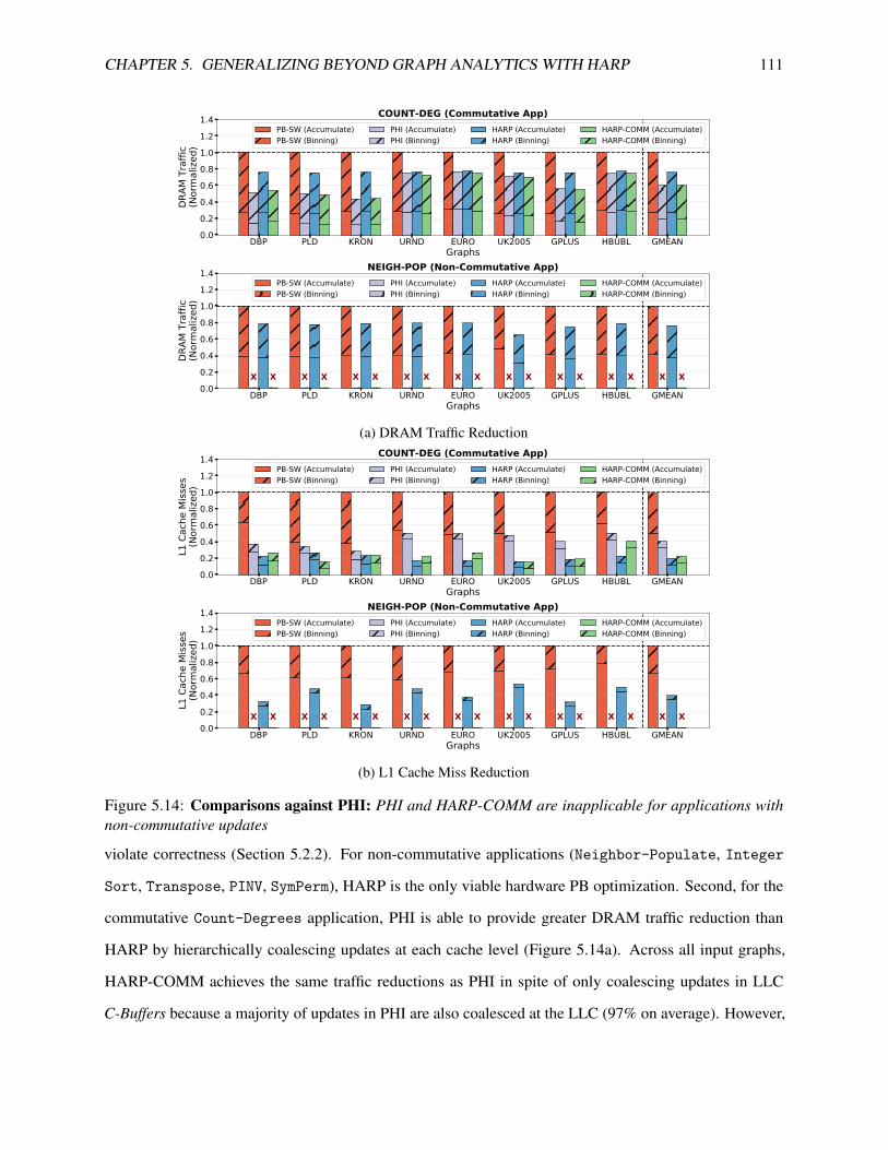
CHAPTER 5. GENERALIZING BEYOND GRAPH ANALYTICS WITH HARP 111
DBP PLD KRON URND EURO UK2005 GPLUS HBUBL GMEANGraphs
0.00.20.40.60.81.01.21.4
DRAM
Tra
ffic
(Nor
mal
ized)
COUNT-DEG (Commutative App)PB-SW (Accumulate)PB-SW (Binning)
PHI (Accumulate)PHI (Binning)
HARP (Accumulate)HARP (Binning)
HARP-COMM (Accumulate)HARP-COMM (Binning)
DBP PLD KRON URND EURO UK2005 GPLUS HBUBL GMEANGraphs
0.00.20.40.60.81.01.21.4
DRAM
Tra
ffic
(Nor
mal
ized)
X X X X X X X X XX X X X X X X X X
NEIGH-POP (Non-Commutative App)PB-SW (Accumulate)PB-SW (Binning)
PHI (Accumulate)PHI (Binning)
HARP (Accumulate)HARP (Binning)
HARP-COMM (Accumulate)HARP-COMM (Binning)
(a) DRAM Traffic Reduction
DBP PLD KRON URND EURO UK2005 GPLUS HBUBL GMEANGraphs
0.00.20.40.60.81.01.21.4
L1 C
ache
Miss
es(N
orm
alize
d)
COUNT-DEG (Commutative App)PB-SW (Accumulate)PB-SW (Binning)
PHI (Accumulate)PHI (Binning)
HARP (Accumulate)HARP (Binning)
HARP-COMM (Accumulate)HARP-COMM (Binning)
DBP PLD KRON URND EURO UK2005 GPLUS HBUBL GMEANGraphs
0.00.20.40.60.81.01.21.4
L1 C
ache
Miss
es(N
orm
alize
d)
X X X X X X X X XX X X X X X X X X
NEIGH-POP (Non-Commutative App)PB-SW (Accumulate)PB-SW (Binning)
PHI (Accumulate)PHI (Binning)
HARP (Accumulate)HARP (Binning)
HARP-COMM (Accumulate)HARP-COMM (Binning)
(b) L1 Cache Miss Reduction
Figure 5.14: Comparisons against PHI: PHI and HARP-COMM are inapplicable for applications withnon-commutative updates
violate correctness (Section 5.2.2). For non-commutative applications (Neighbor-Populate, Integer
Sort, Transpose, PINV, SymPerm), HARP is the only viable hardware PB optimization. Second, for the
commutative Count-Degrees application, PHI is able to provide greater DRAM traffic reduction than
HARP by hierarchically coalescing updates at each cache level (Figure 5.14a). Across all input graphs,
HARP-COMM achieves the same traffic reductions as PHI in spite of only coalescing updates in LLC
C-Buffers because a majority of updates in PHI are also coalesced at the LLC (97% on average). However,

CHAPTER 5. GENERALIZING BEYOND GRAPH ANALYTICS WITH HARP 112
PHI’s (and HARP-COMM’s) traffic reductions are tied to highly skewed input graphs and input graphs with
lower temporal reuse in caches (URND, EURO, UK2005, HBUBL) see lesser relative benefit from PHI
compared to HARP. The result shows that PHI’s improvements are tied to the amount of temporal locality
that can be mined from caches and applications with no temporal reuse (e.g. PINV) are unlikely to receive
benefits from PHI. Third, HARP consistently reduces L1 caches misses compared to PHI (Figure 5.14b).
HARP minimizes L1 misses by choosing the optimal number of bins for the Accumulate phase whereas
PHI’s L1 miss reductions are a product of coalescing updates and reducing the number of tuples to be read
from bins. For graphs with low coalescing opportunity (URND, EURO, UK2005, HBUBL), the Accumulate
phase in PHI suffers from choosing a sub-optimal number of bins (as in PB-SW) and provides limited L1
miss reduction over PB-SW.
In summary, HARP is a more general PB optimization compared to PHI because it applies to both
commutative and non-commutative applications. Additionally, with simple modifications, HARP can be
specialized for commutative updates (HARP-COMM) to combine the benefits of update coalescing (to
achieve similar traffic reductions as PHI) and choosing the optimal number of bins for the Accumulate phase
(improving Accumulate L1 locality compared to PHI).
5.5.5 Rationale for Using PB Over Graph Tiling
In this work, we focused on developing architecture support for extending the performance gains of software
PB. Another popular software-based cache locality optimization is graph-tiling [149, 159, 175, 176, 183]
where an input graph is divided into "sub-graphs" such that the irregular accesses performed while processing
each sub-graph can fit within the LLC. To understand the difference between the PB and Tiling, we compare
PB to CSR-Segmenting 6 [176] (a state-of-the-art 1D tiling solution that has been shown to outperform prior
approaches like GridGraph [183] and X-Stream [149]). Figure 5.15 shows the reduction in execution time
achieved by CSR-Segmenting (Tiling) and PB for the Pagerank application run until convergence. The
shaded portion in the bars represents the initialization overheads of Tiling (constructing the per-tile CSRs)
and PB (allocating memory for bins). Ignoring overheads, PB provides a mean speedup of 1.35x compared to
1.27x from Tiling (PB is particularly effective for sparser inputs as observed in prior work [28]). Additionally,
the initialization overheads of PB are significantly lower compared to Tiling allowing PB to offer a higher net
6We use the GraphIt [178] implementation of CSR-Segmenting

CHAPTER 5. GENERALIZING BEYOND GRAPH ANALYTICS WITH HARP 113
performance improvement. Therefore, we selected PB as the basis for our architecture extensions because
PB is able to provide speedups even after accounting for overheads.
DBP PLD KRON URND EURO HBUBL HTRACE KMER DEL GMEANInputs
0.00.51.01.52.02.53.0
7.5x 5x
Normalized TimeBASE CAGRA PB
Figure 5.15: Comparing PB to Tiling: Ignoring overheads, PB offers competitive performance to Tiling.PB also incurs significantly lower overheads compared to Tiling.
5.6 Related Work
There are four categories of work related to HARP: commutative PB optimizations general PB optimizations,
graph tiling, and graph processing architectures.
PB Optimizations for commutative updates: Prior work specializes PB for applications with commutative
updates. The most related work to HARP is PHI [130], which optimizes applications with irregular commu-
tative updates (Section 5.5.4). Milk [100] is a compiler-based optimization for PB that simplifies writing PB
versions of applications. Using pragmas, programmers specify index and update values to be binned and an
operator for combining updates. Milk allows combining commutative updates to the same index. HARP
could be a target for the Milk compiler, extending HARP’s benefits to new applications. GraFBoost [90]
exploits commutativity in PB for out-of-core graph analytics while HARP targets in-memory analytics.
Compared to these works, HARP is a more general PB optimization because it supports non-commutative
updates and can be specialized for commutative updates (Section 5.5.4).
General PB optimizations: Prior work addressed inefficiencies of software PB. PCP [107] and GPOP [106]
reduce memory traffic in Binning with new graph representations but they incur higher preprocessing
overheads compared to PB. Unfortunately, they increase preprocessing overheads compared to PB limiting
their applicability in scenarios with tight latency requirements. Ozdal et al. [138] propose algorithmic changes
to PB that allow running Binning and Accumulate concurrently and reduce PB’s memory overhead. To
reduce the memory requirements of PB, Ozdal et al. propose algorithmic changes to PB allowing Binning
and Accumulate to run concurrently. HARP could support variations of PB using extensions similar to

CHAPTER 5. GENERALIZING BEYOND GRAPH ANALYTICS WITH HARP 114
Section 5.5.4. Prior works [153, 180] have highlighted the sensitivity of radix partitioning to the number
of partitions (i.e. bins in PB) and demonstrated unexpected performance cliffs. In contrast to PB, HARP
eliminates the need to tune for the bin range parameter by sizing the bin ranges as per each level’s capacity.
Tiling optimizations: Various tiling optimizations exist for graph analytics. Section 5.5.5 compared PB to
graph tiling [149, 159, 175, 176, 183]. Tiling incurs pre-processing overheads (e.g., creating per-tile CSR)
but has low dynamic overheads. In contrast, PB has low pre-processing overhead but suffers from dynamic
overheads for Binning. HARP shares PB’s low pre-processing cost and optimizes away PB’s dynamic
overhead using architecture support.
Architectures for graph processing: HARP follows prior work that propose architecture support for
common graph sub-computations. Minnow [171] provides architecture support for efficient worklist man-
agement [145]. HATS [128] introduces custom hardware for online vertex scheduling to improve locality.
OMEGA [9] tailors scratchpad-based memories to optimize graph analytics on power-law inputs. Graph
processing accelerators [75, 140] optimize common framework operations. Similar to these works, HARP
provides architecture support for Binning to optimize PB.
5.7 Discussion
This chapter focused on optimizing Propagation Blocking (PB), a versatile software-based cache locality
optimization. HARP provides architecture support to eliminate the lingering sources of inefficiencies
in a PB execution and extends PB’s performance benefits across a broad range of workloads (including
graph analytics). Beyond offering high speedups for graph analytics applications (Pagerank and Radii in
Figure 5.10), HARP can also provide end-to-end graph analytics performance because it applies to both
graph processing and pre-processing. To illustrate this point, we compare the cost of executing the Pagerank
application directly on an Edgelist 7 compared to Pagerank execution on a CSR (including the cost of
converting from Edgelist to CSR). Figure 5.16 shows the benefits of constructing the CSR as well as the
speedups achieved with accelerating graph processing and pre-processing with PB and HARP. The data
show that even after including the pre-processing cost of constructing a CSR from the Edgelist, running
Pagerank on a CSR yields a mean speedup of 1.8x over hrunning Pagerank directly on an Edgelist. PB
and HARP apply to both the pre-processing and graph processing phases, allowing HARP to increase the
7Most public repositories store graphs in the Edgelist (COO) format [50, 103, 115].

CHAPTER 5. GENERALIZING BEYOND GRAPH ANALYTICS WITH HARP 115
mean end-to-end speedup over Edgelist-based Pagerank to 4.2x. Besides CSR pre-processing, PB (and
HARP) should also be able to optimize the construction of common representations such as DCSR [63] and
CSF [155] due to the similarity in the access patterns of constructing these sparse data structures from a list
of coordinates (COO).
DBP PLD KRON URND EURO GMEANGraphs
0.01.02.03.04.05.06.0
End-
to-e
nd S
peed
up PR-ELEL-to-CSR + PR-CSR
EL-to-CSR (PB-SW) + PR-CSR (PB-SW)EL-to-CSR (HARP) + PR-CSR (HARP)
Figure 5.16: End to end graph analytics speedups with HARP: HARP applies to both graph pre-processing(EdgeList-to-CSR) and graph processing (PageRank)
In conclusion, by targeting the versatile PB optimization (whose sole requirement is that an application
perform irregular updates), HARP is able to improve cache locality for a broad range of applications beyond
just graph analytics workloads.

Chapter 6
Conclusions
In this final chapter, we identify the common recurring themes that span across the works proposed in this
thesis (Chapters 2 to 5). We also identify some future research directions to generalize the ideas developed in
this thesis to broader contexts. Finally, we conclude with some remarks on how the different works presented
in this thesis solve the fundamental problem of in-memory graph analytics – poor cache locality.
6.1 Cross-cutting Themes
Two themes consistently appear across all our proposed works – 1) the importance of considering preprocess-
ing overheads and 2) high performance sensitivity to input graphs.
6.1.1 Importance of Considering Preprocessing Overheads
Preprocessing costs have played a significant role in every idea proposed in this thesis. In Chapter 2, we
saw that while sophisticated graph reordering techniques provide high speedups they also incur extreme
overheads (Table 2.1); limiting the viability of such reordering techniques. Even among lightweight reordering
techniques, our characterization revealed that once we include preprocessing (i.e. reordering) costs it is
not obvious whether graph reordering will always provide a net benefit (Figure 2.2). In Chapter 3, we saw
that the most compelling argument for using RADAR was that it was able to eliminate atomics without
impacting work-efficiency (in contrast to prior optimizations). Besides the work-efficiency benefits, the
low preprocessing overheads of RADAR (having to construct only the CSR and not the CSR and CSC) is
another major factor that allows RADAR to provide a higher net speedup compared to the Push-Pull direction
116

CHAPTER 6. CONCLUSIONS 117
switching optimization (Figure 3.7). In Chapter 4, we saw that the Rereference Matrix allowed P-OPT to
perform near-optimal cache replacement and significantly outperform existing state-of-the-art replacement
policies. It was crucially important for the Rereference Matrix construction cost to be very low (Table 4.4)
because otherwise the overhead of building the Rereference Matrix could have completely overshadowed
the locality improvements from P-OPT (Figure 4.10). Finally, in Chapter 5, we saw that HARP applies to
graph analytics workloads and graph preprocessing tasks. We included graph preprocessing as one of the
target workloads for HARP because prior work has showed that even a basic preprocessing task such as
constructing a CSR from an Edgelist accounts for 48-97% of the total execution time [19]. Targeting graph
preprocessing (in addition to graph processing) allowed HARP to improve end-to-end performance of graph
analytics (Figure 5.16).
The main takeaway from all the above projects is that it is always important to consider the preprocessing
overheads of any graph (locality) optimization. The peril of ignoring preprocessing overheads is that we may
overestimate the benefits of any given optimization (or, even worse, refer to a system that provides a net
slowdown as an optimization).
6.1.2 Performance Sensitivity to Input Graphs
The second major theme across our proposed works is the high performance sensitivity to different input
graphs. Chapters 2 and 3 are entirely motivated by the unique performance trends of graph analytics on power-
law graphs. These chapters demonstrated that we can build useful software cache locality optimizations
by leveraging a common structural property of input graphs. Sensitivity to input graphs also appears in
our architectural optimizations (Chapters 4 and 5). Even though the P-OPT and HARP optimizations are
input-graph agnostic (i.e. the benefits are not restricted to a specific type of input graphs), the magnitude
of speedups offered by these optimizations does depend on the input graph to a small extent. Having a
better understanding of how properties of input graphs affect performance offers a few advantages (even
for input-agnostic graph optimizations). First, it can help set our expectations about the extent of benefits
received from any given locality optimization (for example, bounded-degree graphs such as road networks
have a low average degree and, hence, present low cache reuse opportunity. In contrast, power-law graphs
have significant cache reuse corresponding to the hub vertices). Second, in the accelerator era, having
an understanding of how properties of the input graph affect performance can guide the design of new

CHAPTER 6. CONCLUSIONS 118
tiling mechanisms or reordering schemes to improve the efficiency of graph analytics/sparse linear algebra
accelerators for common inputs [172, 179].
6.2 Future Research Directions
We identify two future research directions for extending the ideas proposed in this thesis to new applications,
inputs, and architectures.
6.2.1 Expanding the Scope of Graph Reordering
Chapter 2 showed how graph reordering is effective at reducing Last Level Cache and TLB misses (Figure 2.5).
Chapter 3 showed that graph reordering (when combined with data duplication) eliminates expensive atomic
updates, providing the best scalability with RADAR (Figure 3.10). To summarize the ideas presented in
these chapters, we leveraged input graphs with power-law degree distribution to improve cache locality
and multi-core scalability. This leads to the question – can we expand the scope of graph reordering to
incorporate a broader set of graphs and target a broader set of architectural optimizations?
On the inputs front, we have already seen an example of a graph reordering technique that leverages
structural properties besides power-law degree distribution – Rabbit Ordering exploits the community
structure present in some graphs (Section 2.2.1). Prior work has also identified specific reordering techniques
for bounded-degree graphs such as road-networks [92]. Going forward, as new graph analytics applications
emerge they will bring their own set of input graphs with unique structural properties (for example, De
Bruijn graphs in genomics [66]). Therefore, a valuable research contribution would be to catalog the
different types of degree distributions observed in typical, real-world input graphs and compile a menu
of reordering techniques that is best suited for each degree distribution. The knowledge of how different
structural properties of input graphs affect performance can lead to a more aggressive version of selective
graph reordering, where instead of choosing whether or not to apply reordering (as in Chapter 2) we can
choose the best reordering technique for any given input graph.
On the architectural optimizations front, we can expand the scope of graph reordering techniques to go
beyond improving data reuse in on-chip caches and improving parallel scalability. For example, prior work
has observed that partitioning a graph can be viewed as a form of graph reordering [164] and partitioning
schemes have been shown to significantly reduce network traffic in distributed graph analytics [69]. In

CHAPTER 6. CONCLUSIONS 119
increasingly NUMA architectures (for example, sockets in multi-core CPUs or multi-chip modules in
GPUs [14]), coming up with good partitions (through reordering) can reduce expensive on-chip network
traffic. Additionally, graph reordering could also target other goals such as ordering vertices into blocks so as
to improve SIMD/SIMT efficiency.
Besides inputs and architectural optimizations, the design space of graph reordering techniques can
also include the dimension of reordering overhead. As far as reordering overheads are concerned it is the
downstream graph analytics application that ultimately decides whether the overhead of any given reordering
technique is feasible or not. Therefore, there is value in developing a broad range of reordering techniques,
each providing varying levels of data reuse and reordering overheads. Another research direction would be to
investigate architecture support to reduce reordering overheads (as illustrated with HARP in Chapter 5). With
sufficient architecture support, previously inapplicable, sophisticated reordering techniques may suddenly
become viable in many more scenarios. In summary, the interplay of structural properties of input graphs and
architectural optimizations coupled with constraints on reordering overhead opens up a rich design space for
developing future reordering techniques.
6.2.2 Transparent Scaling of GPU-based Graph Analytics
With a higher number of cores and higher memory bandwidth, GPU-based graph analytics can provide
significant speedups compared to graph analytics on multi-core CPUs [39]. However, a fundamental
limitation of GPU-based graph analytics is that GPUs have smaller main memory capacity relative to large
multi-core processors which limits the size of the largest graph that can be analyzed using a single GPU.
The most common solution to process large graphs using GPUs is to rely on distributed, multi-GPU graph
analytics [87, 89, 141] where the input graph is partitioned across multiple GPUs. While effective at scaling
to large input graphs, multi-GPU graph analytics requires graph partitioning which can impose preprocessing
overheads and complicate the programming model.
To avoid the preprocessing and programmability overheads of multi-GPU graph analytics, graph analytics
frameworks could use Unified Virtual Memory (UVM) where the host (CPU) and GPU device have a shared
view of memory [64]. With UVM, the hardware is responsible for transparently move pages between the
larger CPU memory and the smaller GPU memory on demand; alleviating the burden of data migration
from the programmer. In theory, UVM should trivially allow analyzing large input graphs using just a single

CHAPTER 6. CONCLUSIONS 120
GPU. However, in practise, fine-grained irregular memory accesses (as is typical in graph analytics) leads to
inefficient page migration and causes systems using UVM to incur a huge performance penalty [182]. Due
to the high overheads of UVM for irregular memory accesses, (to the best of our knowledge) no existing
GPU-based graph analytics system relies UVM to scale to larger input graphs. Therefore, we have an
opportunity to improve UVM performance for irregular memory accesses so as to allow GPU graph analytics
to transparently scale to larger input graphs.
The primary reason for poor performance of UVM on irregular memory accesses is the poor locality of
pages that are migrated into the GPU memory. UVM typically uses a simple LRU replacement policy to
decide which pages need to be evicted back to the CPU memory because that is sufficient for applications
with more regular access patterns [8, 64]. However, as we saw in Chapter 4, LRU is a bad fit for irregular
memory accesses. Fortunately, the UVM context is very similar to the system that P-OPT was designed
for – the GPU memory is equivalent to the "LLC", the CPU memory is equivalent to the "DRAM", and
the page size is equivalent to "cache line size" for the Rereference Matrix. Given the similarity between
the two scenarios, a modified version of P-OPT should be able maximize locality of pages in the GPU
memory by making near-optimal replacement decisions. As part of future work, we plan to evaluate such
a P-OPT-equipped UVM system and compare its effectiveness relative to distributed, multi-GPU graph
analytics.
6.3 Final Remarks
At the beginning of this thesis, we highlighted the poor cache locality of graph analytics workloads caused by
irregular memory accesses. The main insight of this thesis was that the different sources of irregularity in
graph analytics workloads contain valuable information that can be used to design cache locality optimizations.
As proof, we developed software and hardware based cache locality optimizations by leveraging common
structural properties of input graphs (Chapters 2 and 3), popular graph representations (Chapter 4) and
application access patterns (Chapter 5). The solutions proposed in this thesis highlight the abundant structure
within the irregular memory accesses in graph analytics workloads and, more importantly, showcase the
benefits of carefully analyzing common structural properties and representations of inputs while designing
graph locality optimizations.

Bibliography
[1] “Amazon ec2 high memory instances,” https://aws.amazon.com/ec2/instance-types/high-memory/,
accessed: 2021-05-12.
[2] “Likwid Marker API with C/C++,” https://github.com/RRZE-HPC/likwid/wiki/TutorialMarkerC#
problems, accessed: 2018-05-25.
[3] “Linux scheduling quantum,” https://man7.org/linux/man-pages/man2/sched_rr_get_interval.2.html,
accessed: 2021-04-16.
[4] “Pagerank use at google,” https://twitter.com/methode/status/829755916895535104?s=20, accessed:
2021-05-10.
[5] “Uber’s routing engine,” https://eng.uber.com/engineering-routing-engine/, accessed: 2021-05-10.
[6] “Cache Replacement Championship,” https://crc2.ece.tamu.edu/, 2020, [Online; accessed 31-July-
2020].
[7] “Intel CAT,” https://github.com/intel/intel-cmt-cat, 2020, [Online; accessed 17-April-2020].
[8] “Nvidia Unified Memory,” https://on-demand.gputechconf.com/gtc/2018/presentation/s8430-
everything-you-need-to-know-about-unified-memory.pdf, 2021, [Online; accessed 21-May-2021].
[9] A. Addisie, H. Kassa, O. Matthews, and V. Bertacco, “Heterogeneous memory subsystem for natural
graph analytics,” in 2018 IEEE International Symposium on Workload Characterization (IISWC),
2018, pp. 134–145.
[10] S. Ainsworth and T. M. Jones, “Graph prefetching using data structure knowledge,” in Proceedings of
the 2016 International Conference on Supercomputing, 2016, pp. 1–11.
[11] S. Ainsworth and T. M. Jones, “Software prefetching for indirect memory accesses,” in 2017
IEEE/ACM International Symposium on Code Generation and Optimization (CGO). IEEE, 2017, pp.
305–317.
[12] M. J. Anderson, N. Sundaram, N. Satish, M. M. A. Patwary, T. L. Willke, and P. Dubey, “Graph-
pad: Optimized graph primitives for parallel and distributed platforms,” in Parallel and Distributed
Processing Symposium, 2016 IEEE International. IEEE, 2016, pp. 313–322.
121

BIBLIOGRAPHY 122
[13] J. Arai, H. Shiokawa, T. Yamamuro, M. Onizuka, and S. Iwamura, “Rabbit order: Just-in-time parallel
reordering for fast graph analysis,” in Parallel and Distributed Processing Symposium, 2016 IEEE
International. IEEE, 2016, pp. 22–31.
[14] A. Arunkumar, E. Bolotin, B. Cho, U. Milic, E. Ebrahimi, O. Villa, A. Jaleel, C.-J. Wu, and D. Nellans,
“Mcm-gpu: Multi-chip-module gpus for continued performance scalability,” ACM SIGARCH Computer
Architecture News, vol. 45, no. 2, pp. 320–332, 2017.
[15] D. H. Bailey, E. Barszcz, J. T. Barton, D. S. Browning, R. L. Carter, L. Dagum, R. A. Fatoohi,
P. O. Frederickson, T. A. Lasinski, R. S. Schreiber et al., “The nas parallel benchmarks summary
and preliminary results,” in Supercomputing’91: Proceedings of the 1991 ACM/IEEE conference on
Supercomputing. IEEE, 1991, pp. 158–165.
[16] V. Balaji, N. Crago, A. Jaleel, and B. Lucia, “P-opt: Practical optimal cache replacement for graph
analytics,” in 2021 IEEE International Symposium on High-Performance Computer Architecture
(HPCA). IEEE, 2021, pp. 668–681.
[17] V. Balaji and B. Lucia, “When is graph reordering an optimization? studying the effect of lightweight
graph reordering across applications and input graphs,” in 2018 IEEE International Symposium on
Workload Characterization (IISWC). IEEE, 2018, pp. 203–214.
[18] V. Balaji and B. Lucia, “Combining data duplication and graph reordering to accelerate parallel graph
processing,” in Proceedings of the 28th International Symposium on High-Performance Parallel and
Distributed Computing, 2019, pp. 133–144.
[19] V. Balaji and B. Lucia, “Optimizing graph processing and preprocessing with hardware assisted
propagation blocking,” arXiv preprint arXiv:2011.08451, 2020.
[20] V. Balaji, B. Lucia, and R. Marculescu, “Overcoming the data-flow limit on parallelism with structural
approximation,” WAX 2016, 2016.
[21] V. Balaji, D. Tirumala, and B. Lucia, “Flexible support for fast parallel commutative updates,” arXiv
preprint arXiv:1709.09491, 2017.
[22] V. Balaji, D. Tirumala, and B. Lucia, “Poster: An architecture and programming model for accelerating
parallel commutative computations via privatization,” ACM SIGPLAN Notices, vol. 52, no. 8, pp.
431–432, 2017.
[23] J. Banerjee, W. Kim, S.-J. Kim, and J. F. Garza, “Clustering a dag for cad databases,” IEEE Transac-
tions on Software Engineering, vol. 14, no. 11, pp. 1684–1699, 1988.
[24] A.-L. Barabási, “Scale-free networks: a decade and beyond,” science, vol. 325, no. 5939, pp. 412–413,
2009.

BIBLIOGRAPHY 123
[25] A. Basak, S. Li, X. Hu, S. M. Oh, X. Xie, L. Zhao, X. Jiang, and Y. Xie, “Analysis and optimization of
the memory hierarchy for graph processing workloads,” in 2019 IEEE International Symposium on
High Performance Computer Architecture (HPCA). IEEE, 2019, pp. 373–386.
[26] S. Beamer, K. Asanovic, and D. Patterson, “Direction-optimizing breadth-first search,” Scientific
Programming, vol. 21, no. 3-4, pp. 137–148, 2013.
[27] S. Beamer, K. Asanovic, and D. Patterson, “Locality exists in graph processing: Workload charac-
terization on an ivy bridge server,” in Workload Characterization (IISWC), 2015 IEEE International
Symposium on. IEEE, 2015, pp. 56–65.
[28] S. Beamer, K. Asanovic, and D. Patterson, “Reducing pagerank communication via propagation
blocking,” in Parallel and Distributed Processing Symposium (IPDPS), 2017 IEEE International.
IEEE, 2017, pp. 820–831.
[29] S. Beamer, K. Asanovic, and D. A. Patterson, “The GAP benchmark suite,” CoRR, vol.
abs/1508.03619, 2015. [Online]. Available: http://arxiv.org/abs/1508.03619
[30] L. A. Belady, “A study of replacement algorithms for a virtual-storage computer,” IBM Systems journal,
vol. 5, no. 2, pp. 78–101, 1966.
[31] M. Besta and T. Hoefler, “Accelerating irregular computations with hardware transactional memory
and active messages,” in Proceedings of the 24th International Symposium on High-Performance
Parallel and Distributed Computing. ACM, 2015, pp. 161–172.
[32] M. Besta, M. Podstawski, L. Groner, E. Solomonik, and T. Hoefler, “To push or to pull: On reducing
communication and synchronization in graph computations,” in 26th International Symposium on
High-Performance Parallel and Distributed Computing (HPDC’17), 2017.
[33] P. Boldi, B. Codenotti, M. Santini, and S. Vigna, “Ubicrawler: A scalable fully distributed web crawler,”
Software: Practice & Experience, vol. 34, no. 8, pp. 711–726, 2004.
[34] P. Boldi, M. Rosa, M. Santini, and S. Vigna, “Layered label propagation: A multiresolution coordinate-
free ordering for compressing social networks,” in Proceedings of the 20th international conference
on World wide web. ACM, 2011, pp. 587–596.
[35] S. Brin and L. Page, “The anatomy of a large-scale hypertextual web search engine,” in Proceedings
of the Seventh International Conference on World Wide Web 7, ser. WWW7. Amsterdam, The
Netherlands, The Netherlands: Elsevier Science Publishers B. V., 1998, pp. 107–117. [Online].
Available: http://dl.acm.org/citation.cfm?id=297805.297827
[36] A. D. Broido and A. Clauset, “Scale-free networks are rare,” Nature communications, vol. 10, no. 1,
pp. 1–10, 2019.
BIBLIOGRAPHY 124
[37] D. Buono, F. Petrini, F. Checconi, X. Liu, X. Que, C. Long, and T.-C. Tuan, “Optimizing sparse
matrix-vector multiplication for large-scale data analytics,” in Proceedings of the 2016 International
Conference on Supercomputing. ACM, 2016, p. 37.
[38] T. E. Carlson, W. Heirman, and L. Eeckhout, “Sniper: Exploring the level of abstraction
for scalable and accurate parallel multi-core simulation,” in Proceedings of 2011 International
Conference for High Performance Computing, Networking, Storage and Analysis, ser. SC
’11. New York, NY, USA: Association for Computing Machinery, 2011. [Online]. Available:
https://doi.org/10.1145/2063384.2063454
[39] S. Che, B. M. Beckmann, S. K. Reinhardt, and K. Skadron, “Pannotia: Understanding irregular gpgpu
graph applications,” in 2013 IEEE International Symposium on Workload Characterization (IISWC).
IEEE, 2013, pp. 185–195.
[40] R. Chen, J. Shi, Y. Chen, and H. Chen, “Powerlyra: Differentiated graph computation and partitioning
on skewed graphs,” in Proceedings of the Tenth European Conference on Computer Systems. ACM,
2015, p. 1.
[41] Y.-D. Chen, H. Chen, and C.-C. King, “Social network analysis for contact tracing,” in Infectious
Disease Informatics and Biosurveillance. Springer, 2011, pp. 339–358.
[42] R. Cheng, J. Hong, A. Kyrola, Y. Miao, X. Weng, M. Wu, F. Yang, L. Zhou, F. Zhao, and E. Chen,
“Kineograph: taking the pulse of a fast-changing and connected world,” in Proceedings of the 7th ACM
european conference on Computer Systems, 2012, pp. 85–98.
[43] F. Chierichetti, R. Kumar, S. Lattanzi, M. Mitzenmacher, A. Panconesi, and P. Raghavan, “On
compressing social networks,” in Proceedings of the 15th ACM SIGKDD international conference on
Knowledge discovery and data mining. ACM, 2009, pp. 219–228.
[44] A. Ching, S. Edunov, M. Kabiljo, D. Logothetis, and S. Muthukrishnan, “One trillion edges: Graph
processing at facebook-scale,” Proceedings of the VLDB Endowment, vol. 8, no. 12, pp. 1804–1815,
2015.
[45] T. H. Cormen, C. E. Leiserson, R. L. Rivest, and C. Stein, Introduction to algorithms. MIT press,
2009.
[46] L. Dagum and R. Menon, “Openmp: an industry standard api for shared-memory programming,” IEEE
computational science and engineering, vol. 5, no. 1, pp. 46–55, 1998.
[47] R. Dathathri, G. Gill, L. Hoang, H.-V. Dang, A. Brooks, N. Dryden, M. Snir, and K. Pingali, “Gluon:
A communication-optimizing substrate for distributed heterogeneous graph analytics,” in Proceedings
of the 39th ACM SIGPLAN Conference on Programming Language Design and Implementation, 2018,
pp. 752–768.
BIBLIOGRAPHY 125
[48] R. Dathathri, G. Gill, L. Hoang, V. Jatala, K. Pingali, V. K. Nandivada, H.-V. Dang, and M. Snir,
“Gluon-async: A bulk-asynchronous system for distributed and heterogeneous graph analytics,” in
2019 28th International Conference on Parallel Architectures and Compilation Techniques (PACT).
IEEE, 2019, pp. 15–28.
[49] T. A. Davis, “Algorithm 1000: Suitesparse: Graphblas: Graph algorithms in the language of sparse
linear algebra,” ACM Transactions on Mathematical Software (TOMS), vol. 45, no. 4, pp. 1–25, 2019.
[50] T. A. Davis and Y. Hu, “The university of florida sparse matrix collection,” ACM Transactions on
Mathematical Software (TOMS), vol. 38, no. 1, p. 1, 2011.
[51] T. A. Davis and Y. Hu, “The university of florida sparse matrix collection,” ACM Transactions on
Mathematical Software (TOMS), vol. 38, no. 1, p. 1, 2011.
[52] L. Dhulipala, G. E. Blelloch, and J. Shun, “Theoretically efficient parallel graph algorithms can be fast
and scalable,” ACM Transactions on Parallel Computing (TOPC), vol. 8, no. 1, pp. 1–70, 2021.
[53] I. D. Direct, “I/o technology (intel ddio) a primer,” 2012.
[54] J. Dongarra, M. A. Heroux, and P. Luszczek, “Hpcg benchmark: a new metric for ranking high
performance computing systems,” Knoxville, Tennessee, pp. 1–11, 2015.
[55] N. Duong, D. Zhao, T. Kim, R. Cammarota, M. Valero, and A. V. Veidenbaum, “Improving cache
management policies using dynamic reuse distances,” in 2012 45th Annual IEEE/ACM International
Symposium on Microarchitecture. IEEE, 2012, pp. 389–400.
[56] D. Easley and J. Kleinberg, Networks, crowds, and markets: Reasoning about a highly connected
world. Cambridge University Press, 2010.
[57] D. Eswaran and C. Faloutsos, “Sedanspot: Detecting anomalies in edge streams,” in 2018 IEEE
International Conference on Data Mining (ICDM). IEEE, 2018, pp. 953–958.
[58] D. Eswaran, C. Faloutsos, S. Guha, and N. Mishra, “Spotlight: Detecting anomalies in streaming
graphs,” in Proceedings of the 24th ACM SIGKDD International Conference on Knowledge Discovery
& Data Mining, 2018, pp. 1378–1386.
[59] P. Faldu, J. Diamond, and B. Grot, “A closer look at lightweight graph reordering,” in IISWC, 2019.
[60] P. Faldu, J. Diamond, and B. Grot, “Domain-specialized cache management for graph analytics,” in
2020 IEEE International Symposium on High Performance Computer Architecture (HPCA). IEEE,
2020, pp. 234–248.
[61] P. Faldu and B. Grot, “Leeway: Addressing variability in dead-block prediction for last-level caches,”
in 2017 26th International Conference on Parallel Architectures and Compilation Techniques (PACT).
IEEE, 2017, pp. 180–193.

BIBLIOGRAPHY 126
[62] A. Farshin, A. Roozbeh, G. Q. Maguire Jr, and D. Kostic, “Make the most out of last level cache in
intel processors,” in Proceedings of the Fourteenth EuroSys Conference 2019, 2019, pp. 1–17.
[63] D. Fujiki, N. Chatterjee, D. Lee, and M. O’Connor, “Near-memory data transformation for efficient
sparse matrix multi-vector multiplication,” in Proceedings of the International Conference for High
Performance Computing, Networking, Storage and Analysis, 2019, pp. 1–17.
[64] D. Ganguly, Z. Zhang, J. Yang, and R. Melhem, “Interplay between hardware prefetcher and page
eviction policy in cpu-gpu unified virtual memory,” in Proceedings of the 46th International Symposium
on Computer Architecture, 2019, pp. 224–235.
[65] R. Geisberger, P. Sanders, D. Schultes, and D. Delling, “Contraction hierarchies: Faster and simpler
hierarchical routing in road networks,” in International Workshop on Experimental and Efficient
Algorithms. Springer, 2008, pp. 319–333.
[66] E. Georganas, A. Buluç, J. Chapman, L. Oliker, D. Rokhsar, and K. Yelick, “Parallel de bruijn graph
construction and traversal for de novo genome assembly,” in SC’14: Proceedings of the International
Conference for High Performance Computing, Networking, Storage and Analysis. IEEE, 2014, pp.
437–448.
[67] E. Georganas, R. Egan, S. Hofmeyr, E. Goltsman, B. Arndt, A. Tritt, A. Buluç, L. Oliker, and
K. Yelick, “Extreme scale de novo metagenome assembly,” in SC18: International Conference for
High Performance Computing, Networking, Storage and Analysis. IEEE, 2018, pp. 122–134.
[68] G. Gill, R. Dathathri, L. Hoang, R. Peri, and K. Pingali, “Single machine graph analytics on massive
datasets using intel optane dc persistent memory,” Proceedings of the VLDB Endowment, vol. 13,
no. 8.
[69] G. Gill, R. Dathathri, L. Hoang, and K. Pingali, “A study of partitioning policies for graph analytics on
large-scale distributed platforms,” Proceedings of the VLDB Endowment, vol. 12, no. 4, pp. 321–334,
2018.
[70] M. Girvan and M. E. Newman, “Community structure in social and biological networks,” Proceedings
of the national academy of sciences, vol. 99, no. 12, pp. 7821–7826, 2002.
[71] N. Z. Gong and W. Xu, “Reciprocal versus parasocial relationships in online social networks,” Social
Network Analysis and Mining, vol. 4, no. 1, p. 184, 2014.
[72] J. E. Gonzalez, Y. Low, H. Gu, D. Bickson, and C. Guestrin, “Powergraph: Distributed graph-parallel
computation on natural graphs.” in OSDI, vol. 12, no. 1, 2012, p. 2.
[73] P. Gupta, A. Goel, J. Lin, A. Sharma, D. Wang, and R. Zadeh, “Wtf: The who to follow service at
twitter,” in Proceedings of the 22nd international conference on World Wide Web, 2013, pp. 505–514.

BIBLIOGRAPHY 127
[74] N. Hajaj, “Producing a ranking for pages using distances in a web-link graph,” Apr. 24 2018, uS Patent
9,953,049.
[75] T. J. Ham, L. Wu, N. Sundaram, N. Satish, and M. Martonosi, “Graphicionado: A high-performance
and energy-efficient accelerator for graph analytics,” in Microarchitecture (MICRO), 2016 49th Annual
IEEE/ACM International Symposium on. IEEE, 2016, pp. 1–13.
[76] W. L. Hamilton, R. Ying, and J. Leskovec, “Representation learning on graphs: Methods and applica-
tions,” arXiv preprint arXiv:1709.05584, 2017.
[77] M. Han and K. Daudjee, “Giraph unchained: Barrierless asynchronous parallel execution in pregel-like
graph processing systems,” Proceedings of the VLDB Endowment, vol. 8, no. 9, pp. 950–961, 2015.
[78] W. Han, Y. Miao, K. Li, M. Wu, F. Yang, L. Zhou, V. Prabhakaran, W. Chen, and E. Chen, “Chronos:
a graph engine for temporal graph analysis,” in Proceedings of the Ninth European Conference on
Computer Systems, 2014, pp. 1–14.
[79] W.-S. Han, S. Lee, K. Park, J.-H. Lee, M.-S. Kim, J. Kim, and H. Yu, “Turbograph: a fast parallel
graph engine handling billion-scale graphs in a single pc,” in Proceedings of the 19th ACM SIGKDD
international conference on Knowledge discovery and data mining. ACM, 2013, pp. 77–85.
[80] N. Hardavellas, M. Ferdman, B. Falsafi, and A. Ailamaki, “Reactive nuca: near-optimal block
placement and replication in distributed caches,” in Proceedings of the 36th annual international
symposium on Computer architecture, 2009, pp. 184–195.
[81] S. Haria, M. D. Hill, and M. M. Swift, “Devirtualizing memory in heterogeneous systems,” in
Proceedings of the Twenty-Third International Conference on Architectural Support for Programming
Languages and Operating Systems, 2018, pp. 637–650.
[82] M. A. Hassaan, M. Burtscher, and K. Pingali, “Ordered vs. unordered: a comparison of parallelism
and work-efficiency in irregular algorithms,” Acm Sigplan Notices, vol. 46, no. 8, pp. 3–12, 2011.
[83] M. D. Hill, “Three other models of computer system performance,” arXiv preprint arXiv:1901.02926,
2019.
[84] A. Jain and C. Lin, “Back to the future: leveraging belady’s algorithm for improved cache replacement,”
in 2016 ACM/IEEE 43rd Annual International Symposium on Computer Architecture (ISCA). IEEE,
2016, pp. 78–89.
[85] A. Jaleel, W. Hasenplaugh, M. Qureshi, J. Sebot, S. Steely Jr, and J. Emer, “Adaptive insertion
policies for managing shared caches,” in Proceedings of the 17th international conference on Parallel
architectures and compilation techniques, 2008, pp. 208–219.
[86] A. Jaleel, K. B. Theobald, S. C. Steely Jr, and J. Emer, “High performance cache replacement using
re-reference interval prediction (rrip),” ACM SIGARCH Computer Architecture News, vol. 38, no. 3,
pp. 60–71, 2010.

BIBLIOGRAPHY 128
[87] V. Jatala, R. Dathathri, G. Gill, L. Hoang, V. K. Nandivada, and K. Pingali, “A study of graph analytics
for massive datasets on distributed multi-gpus,” in 2020 IEEE International Parallel and Distributed
Processing Symposium (IPDPS). IEEE, 2020, pp. 84–94.
[88] M. C. Jeffrey, S. Subramanian, C. Yan, J. Emer, and D. Sanchez, “Unlocking ordered parallelism with
the swarm architecture,” IEEE Micro, vol. 36, no. 3, pp. 105–117, 2016.
[89] Z. Jia, Y. Kwon, G. Shipman, P. McCormick, M. Erez, and A. Aiken, “A distributed multi-gpu system
for fast graph processing,” Proceedings of the VLDB Endowment, vol. 11, no. 3, pp. 297–310, 2017.
[90] S.-W. Jun, A. Wright, S. Zhang, S. Xu, and Arvind, “Grafboost: Using accelerated flash storage
for external graph analytics,” in Proceedings of the 45th Annual International Symposium on
Computer Architecture, ser. ISCA ’18. IEEE Press, 2018, p. 411–424. [Online]. Available:
https://doi.org/10.1109/ISCA.2018.00042
[91] S.-W. Jun, A. Wright, S. Zhang, S. Xu et al., “Bigsparse: High-performance external graph analytics,”
arXiv preprint arXiv:1710.07736, 2017.
[92] K. I. Karantasis, A. Lenharth, D. Nguyen, M. J. Garzarán, and K. Pingali, “Parallelization of reordering
algorithms for bandwidth and wavefront reduction,” in Proceedings of the International Conference for
High Performance Computing, Networking, Storage and Analysis. IEEE Press, 2014, pp. 921–932.
[93] G. Karypis and V. Kumar, “Metis–unstructured graph partitioning and sparse matrix ordering system,
version 2.0,” 1995.
[94] J. Kepner, P. Aaltonen, D. Bader, A. Buluç, F. Franchetti, J. Gilbert, D. Hutchison, M. Kumar,
A. Lumsdaine, H. Meyerhenke et al., “Mathematical foundations of the graphblas,” in 2016 IEEE
High Performance Extreme Computing Conference (HPEC). IEEE, 2016, pp. 1–9.
[95] J. Kepner, D. Bader, A. Buluç, J. Gilbert, T. Mattson, and H. Meyerhenke, “Graphs, matrices, and the
graphblas: Seven good reasons,” Procedia Computer Science, vol. 51, pp. 2453–2462, 2015.
[96] G. Keramidas, P. Petoumenos, and S. Kaxiras, “Cache replacement based on reuse-distance prediction,”
in 2007 25th International Conference on Computer Design. IEEE, 2007, pp. 245–250.
[97] S. M. Khan, Y. Tian, and D. A. Jimenez, “Sampling dead block prediction for last-level caches,” in
2010 43rd Annual IEEE/ACM International Symposium on Microarchitecture. IEEE, 2010, pp.
175–186.
[98] F. Khorasani, K. Vora, R. Gupta, and L. N. Bhuyan, “Cusha: Vertex-centric graph processing on gpus,”
in Proceedings of the 23rd international symposium on High-performance parallel and distributed
computing, 2014, pp. 239–252.
[99] C. Kim, D. Burger, and S. W. Keckler, “Nonuniform cache architectures for wire-delay dominated
on-chip caches,” IEEE Micro, vol. 23, no. 6, pp. 99–107, 2003.

BIBLIOGRAPHY 129
[100] V. Kiriansky, Y. Zhang, and S. Amarasinghe, “Optimizing indirect memory references with milk,” in
Proceedings of the 2016 International Conference on Parallel Architectures and Compilation, ser.
PACT ’16. New York, NY, USA: Association for Computing Machinery, 2016, p. 299–312. [Online].
Available: https://doi.org/10.1145/2967938.2967948
[101] J. M. Kleinberg, M. Newman, A.-L. Barabási, and D. J. Watts, Authoritative sources in a hyperlinked
environment. Princeton University Press, 2011.
[102] S. Kojaku, L. Hébert-Dufresne, E. Mones, S. Lehmann, and Y.-Y. Ahn, “The effectiveness of backward
contact tracing in networks,” Nature Physics, pp. 1–7, 2021.
[103] J. Kunegis, “Konect: the koblenz network collection,” in Proceedings of the 22nd International
Conference on World Wide Web. ACM, 2013, pp. 1343–1350.
[104] H. Kwak, C. Lee, H. Park, and S. Moon, “What is Twitter, a social network or a news media?” in
WWW ’10: Proceedings of the 19th international conference on World wide web. New York, NY,
USA: ACM, 2010, pp. 591–600.
[105] A. Kyrola, G. E. Blelloch, C. Guestrin et al., “Graphchi: Large-scale graph computation on just a pc.”
in OSDI, vol. 12, 2012, pp. 31–46.
[106] K. Lakhotia, R. Kannan, S. Pati, and V. Prasanna, “Gpop: A scalable cache- and memory-efficient
framework for graph processing over parts,” ACM Trans. Parallel Comput., vol. 7, no. 1, Mar. 2020.
[Online]. Available: https://doi.org/10.1145/3380942
[107] K. Lakhotia, R. Kannan, and V. Prasanna, “Accelerating pagerank using partition-centric processing,”
in 2018 {USENIX} Annual Technical Conference ({USENIX}{ATC} 18), 2018, pp. 427–440.
[108] K. Lakhotia, S. Singapura, R. Kannan, and V. Prasanna, “Recall: Reordered cache aware locality based
graph processing,” in 2017 IEEE 24th International Conference on High Performance Computing
(HiPC). IEEE, 2017, pp. 273–282.
[109] K. Lang, “Finding good nearly balanced cuts in power law graphs,” Preprint, 2004.
[110] D. Lasalle and G. Karypis, “Multi-threaded graph partitioning,” in Proceedings of the 2013
IEEE 27th International Symposium on Parallel and Distributed Processing, ser. IPDPS ’13.
Washington, DC, USA: IEEE Computer Society, 2013, pp. 225–236. [Online]. Available:
https://doi.org/10.1109/IPDPS.2013.50
[111] V. Latora and M. Marchiori, “Efficient behavior of small-world networks,” Physical review letters,
vol. 87, no. 19, p. 198701, 2001.
[112] O. Lehmberg, R. Meusel, and C. Bizer, “Graph structure in the web: aggregated by pay-level domain,”
in Proceedings of the 2014 ACM conference on Web science, 2014, pp. 119–128.

BIBLIOGRAPHY 130
[113] R. Lempel and S. Moran, “Salsa: the stochastic approach for link-structure analysis,” ACM Transac-
tions on Information Systems (TOIS), vol. 19, no. 2, pp. 131–160, 2001.
[114] J. Leskovec, J. Kleinberg, and C. Faloutsos, “Graph evolution: Densification and shrinking diameters,”
ACM transactions on Knowledge Discovery from Data (TKDD), vol. 1, no. 1, pp. 2–es, 2007.
[115] J. Leskovec, A. Krevl, and S. Datasets, “Stanford large network dataset collection, 2011,” URL:
http://snap. stanford. edu/data/index. html, 2014.
[116] J. Leskovec, K. J. Lang, A. Dasgupta, and M. W. Mahoney, “Statistical properties of community
structure in large social and information networks,” in Proceedings of the 17th international conference
on World Wide Web, 2008, pp. 695–704.
[117] Y. Lim, U. Kang, and C. Faloutsos, “Slashburn: Graph compression and mining beyond caveman
communities,” IEEE Transactions on Knowledge and Data Engineering, vol. 26, no. 12, pp. 3077–
3089, 2014.
[118] Y. Low, D. Bickson, J. Gonzalez, C. Guestrin, A. Kyrola, and J. M. Hellerstein, “Distributed graphlab:
a framework for machine learning and data mining in the cloud,” Proceedings of the VLDB Endowment,
vol. 5, no. 8, pp. 716–727, 2012.
[119] C.-K. Luk, R. Cohn, R. Muth, H. Patil, A. Klauser, G. Lowney, S. Wallace, V. J. Reddi, and
K. Hazelwood, “Pin: Building customized program analysis tools with dynamic instrumentation,”
in Proceedings of the 2005 ACM SIGPLAN Conference on Programming Language Design and
Implementation, ser. PLDI ’05. New York, NY, USA: ACM, 2005, pp. 190–200. [Online]. Available:
http://doi.acm.org/10.1145/1065010.1065034
[120] L. Ma, Z. Yang, H. Chen, J. Xue, and Y. Dai, “Garaph: Efficient gpu-accelerated graph processing
on a single machine with balanced replication,” in 2017 {USENIX} Annual Technical Conference
({USENIX}{ATC} 17), 2017, pp. 195–207.
[121] S. Maass, C. Min, S. Kashyap, W. Kang, M. Kumar, and T. Kim, “Mosaic: Processing a trillion-edge
graph on a single machine,” in Proceedings of the Twelfth European Conference on Computer Systems,
2017, pp. 527–543.
[122] G. Malewicz, M. H. Austern, A. J. Bik, J. C. Dehnert, I. Horn, N. Leiser, and G. Czajkowski, “Pregel:
A system for large-scale graph processing,” in Proceedings of the 2010 ACM SIGMOD International
Conference on Management of Data, ser. SIGMOD ’10. New York, NY, USA: ACM, 2010, pp.
135–146. [Online]. Available: http://doi.acm.org/10.1145/1807167.1807184
[123] J. Malicevic, B. Lepers, and W. Zwaenepoel, “Everything you always wanted to know about mul-
ticore graph processing but were afraid to ask,” in 2017 {USENIX} Annual Technical Conference
({USENIX}{ATC} 17), 2017, pp. 631–643.

BIBLIOGRAPHY 131
[124] C. Maurice, N. Le Scouarnec, C. Neumann, O. Heen, and A. Francillon, “Reverse engineering intel
last-level cache complex addressing using performance counters,” in International Symposium on
Recent Advances in Intrusion Detection. Springer, 2015, pp. 48–65.
[125] F. McSherry, M. Isard, and D. G. Murray, “Scalability! but at what cost?” in HotOS, 2015.
[126] R. Meusel, S. Vigna, O. Lehmberg, and C. Bizer, “Graph structure in the web—revisited: a trick of the
heavy tail,” in Proceedings of the 23rd international conference on World Wide Web. ACM, 2014, pp.
427–432.
[127] U. Meyer and P. Sanders, “Delta-stepping: A parallel single source shortest path algorithm,” in
Proceedings of the 6th Annual European Symposium on Algorithms, ser. ESA ’98. London, UK, UK:
Springer-Verlag, 1998, pp. 393–404. [Online]. Available: http://dl.acm.org/citation.cfm?id=647908.
740136
[128] A. Mukkara, N. Beckmann, M. Abeydeera, X. Ma, and D. Sanchez, “Exploiting Locality in Graph
Analytics through Hardware-Accelerated Traversal Scheduling,” in Proceedings of the 51st annual
IEEE/ACM international symposium on Microarchitecture (MICRO-51), October 2018.
[129] A. Mukkara, N. Beckmann, and D. Sanchez, “Cache-guided scheduling: Exploiting caches to maxi-
mize locality in graph processing,” AGP’17, 2017.
[130] A. Mukkara, N. Beckmann, and D. Sanchez, “Phi: Architectural support for synchronization-and
bandwidth-efficient commutative scatter updates,” in Proceedings of the 52nd Annual IEEE/ACM
International Symposium on Microarchitecture, 2019, pp. 1009–1022.
[131] N. Muralimanohar, R. Balasubramonian, and N. P. Jouppi, “Cacti 6.0: A tool to model large caches,”
HP Laboratories, pp. 22–31, 2009.
[132] R. C. Murphy, K. B. Wheeler, B. W. Barrett, and J. A. Ang, “Introducing the graph 500,” Cray Users
Group (CUG), vol. 19, pp. 45–74, 2010.
[133] R. C. Murphy, K. B. Wheeler, B. W. Barrett, and J. A. Ang, “Introducing the graph 500,” Cray Users
Group (CUG), 2010.
[134] D. G. Murray, F. McSherry, R. Isaacs, M. Isard, P. Barham, and M. Abadi, “Naiad: a timely dataflow
system,” in Proceedings of the Twenty-Fourth ACM Symposium on Operating Systems Principles.
ACM, 2013, pp. 439–455.
[135] K. Nagarajan, M. Muniyandi, B. Palani, and S. Sellappan, “Social network analysis methods for
exploring sars-cov-2 contact tracing data,” BMC medical research methodology, vol. 20, no. 1, pp.
1–10, 2020.
[136] L. Nai, Y. Xia, I. G. Tanase, H. Kim, and C.-Y. Lin, “Graphbig: Understanding graph computing in the
context of industrial solutions,” in Proceedings of the International Conference for High Performance
Computing, Networking, Storage and Analysis. ACM, 2015, p. 69.

BIBLIOGRAPHY 132
[137] M. Nicolau, A. J. Levine, and G. Carlsson, “Topology based data analysis identifies a subgroup of
breast cancers with a unique mutational profile and excellent survival,” Proceedings of the National
Academy of Sciences, vol. 108, no. 17, pp. 7265–7270, 2011.
[138] M. M. Ozdal, “Improving efficiency of parallel vertex-centric algorithms for irregular graphs,” IEEE
Transactions on Parallel and Distributed Systems, vol. 30, no. 10, pp. 2265–2282, 2019.
[139] M. M. Ozdal, S. Yesil, T. Kim, A. Ayupov, J. Greth, S. Burns, and O. Ozturk, “Energy efficient
architecture for graph analytics accelerators,” in Proceedings of the 43rd International Symposium
on Computer Architecture, ser. ISCA ’16. Piscataway, NJ, USA: IEEE Press, 2016, pp. 166–177.
[Online]. Available: https://doi.org/10.1109/ISCA.2016.24
[140] M. M. Ozdal, S. Yesil, T. Kim, A. Ayupov, J. Greth, S. Burns, and O. Ozturk, “Energy efficient archi-
tecture for graph analytics accelerators,” in 2016 ACM/IEEE 43rd Annual International Symposium on
Computer Architecture (ISCA). IEEE, 2016, pp. 166–177.
[141] Y. Pan, Y. Wang, Y. Wu, C. Yang, and J. D. Owens, “Multi-gpu graph analytics,” in 2017 IEEE
International Parallel and Distributed Processing Symposium (IPDPS). IEEE, 2017, pp. 479–490.
[142] A. Panwar, S. Bansal, and K. Gopinath, “Hawkeye: Efficient fine-grained os support for huge pages,” in
Proceedings of the Twenty-Fourth International Conference on Architectural Support for Programming
Languages and Operating Systems, 2019, pp. 347–360.
[143] R. Pearce, M. Gokhale, and N. M. Amato, “Faster parallel traversal of scale free graphs at extreme
scale with vertex delegates,” in High Performance Computing, Networking, Storage and Analysis,
SC14: International Conference for. IEEE, 2014, pp. 549–559.
[144] J. Petit, “Experiments on the minimum linear arrangement problem,” Journal of Experimental Algo-
rithmics (JEA), vol. 8, pp. 2–3, 2003.
[145] K. Pingali, D. Nguyen, M. Kulkarni, M. Burtscher, M. A. Hassaan, R. Kaleem, T.-H. Lee, A. Lenharth,
R. Manevich, M. Méndez-Lojo et al., “The tao of parallelism in algorithms,” in ACM Sigplan Notices,
vol. 46, no. 6. ACM, 2011, pp. 12–25.
[146] V. Prabhakaran, M. Wu, X. Weng, F. McSherry, L. Zhou, and M. Haridasan, “Managing large graphs
on multi-cores with graph awareness,” 2012.
[147] M. K. Qureshi and Y. N. Patt, “Utility-based cache partitioning: A low-overhead, high-performance,
runtime mechanism to partition shared caches,” in 2006 39th Annual IEEE/ACM International Sympo-
sium on Microarchitecture (MICRO’06). IEEE, 2006, pp. 423–432.
[148] S. Rahman, N. Abu-Ghazaleh, and R. Gupta, “Graphpulse: An event-driven hardware accelerator
for asynchronous graph processing,” in 2020 53rd Annual IEEE/ACM International Symposium on
Microarchitecture (MICRO). IEEE, 2020, pp. 908–921.
BIBLIOGRAPHY 133
[149] A. Roy, I. Mihailovic, and W. Zwaenepoel, “X-stream: Edge-centric graph processing using streaming
partitions,” in Proceedings of the Twenty-Fourth ACM Symposium on Operating Systems Principles.
ACM, 2013, pp. 472–488.
[150] L. Rudolph and Z. Segall, “Dynamic decentralized cache schemes for mimd parallel processors,”
SIGARCH Comput. Archit. News, vol. 12, no. 3, pp. 340–347, Jan. 1984. [Online]. Available:
http://doi.acm.org/10.1145/773453.808203
[151] S. Salihoglu and J. Widom, “Gps: A graph processing system,” in Proceedings of the 25th International
Conference on Scientific and Statistical Database Management, ser. SSDBM. New York, NY, USA:
ACM, 2013, pp. 22:1–22:12. [Online]. Available: http://doi.acm.org/10.1145/2484838.2484843
[152] N. Satish, N. Sundaram, M. M. A. Patwary, J. Seo, J. Park, M. A. Hassaan, S. Sengupta, Z. Yin, and
P. Dubey, “Navigating the maze of graph analytics frameworks using massive graph datasets,” in
Proceedings of the 2014 ACM SIGMOD international conference on Management of data. ACM,
2014, pp. 979–990.
[153] F. M. Schuhknecht, P. Khanchandani, and J. Dittrich, “On the surprising difficulty of simple things:
the case of radix partitioning,” Proceedings of the VLDB Endowment, vol. 8, no. 9, pp. 934–937, 2015.
[154] J. Shun and G. E. Blelloch, “Ligra: a lightweight graph processing framework for shared memory,” in
ACM Sigplan Notices, vol. 48, no. 8. ACM, 2013, pp. 135–146.
[155] S. Smith and G. Karypis, “Tensor-matrix products with a compressed sparse tensor,” in Proceedings of
the 5th Workshop on Irregular Applications: Architectures and Algorithms, 2015, pp. 1–7.
[156] I. Stanton and G. Kliot, “Streaming graph partitioning for large distributed graphs,” in Proceedings of
the 18th ACM SIGKDD international conference on Knowledge discovery and data mining. ACM,
2012, pp. 1222–1230.
[157] J. Sun, H. Vandierendonck, and D. S. Nikolopoulos, “Accelerating graph analytics by utilising the
memory locality of graph partitioning,” in Parallel Processing (ICPP), 2017 46th International
Conference on. IEEE, 2017, pp. 181–190.
[158] J. Sun, H. Vandierendonck, and D. S. Nikolopoulos, “Accelerating graph analytics by utilising the
memory locality of graph partitioning,” in Parallel Processing (ICPP), 2017 46th International
Conference on. IEEE, 2017, pp. 181–190.
[159] J. Sun, H. Vandierendonck, and D. S. Nikolopoulos, “Graphgrind: addressing load imbalance of graph
partitioning,” in Proceedings of the International Conference on Supercomputing. ACM, 2017, p. 16.
[160] N. Sundaram, N. Satish, M. M. A. Patwary, S. R. Dulloor, M. J. Anderson, S. G. Vadlamudi, D. Das,
and P. Dubey, “Graphmat: High performance graph analytics made productive,” Proceedings of the
VLDB Endowment, vol. 8, no. 11, pp. 1214–1225, 2015.

BIBLIOGRAPHY 134
[161] M. Sutton, T. Ben-Nun, and A. Barak, “Optimizing parallel graph connectivity computation via
subgraph sampling,” in 2018 IEEE International Parallel and Distributed Processing Symposium
(IPDPS). IEEE, 2018, pp. 12–21.
[162] J. Treibig, G. Hager, and G. Wellein, “Likwid: A lightweight performance-oriented tool suite for
x86 multicore environments,” in Parallel Processing Workshops (ICPPW), 2010 39th International
Conference on. IEEE, 2010, pp. 207–216.
[163] C. Tsourakakis, C. Gkantsidis, B. Radunovic, and M. Vojnovic, “Fennel: Streaming graph partitioning
for massive scale graphs,” in Proceedings of the 7th ACM International Conference on Web Search
and Data Mining, ser. WSDM ’14. New York, NY, USA: ACM, 2014, pp. 333–342. [Online].
Available: http://doi.acm.org/10.1145/2556195.2556213
[164] H. Wei, J. X. Yu, C. Lu, and X. Lin, “Speedup graph processing by graph ordering,” in Proceedings of
the 2016 International Conference on Management of Data. ACM, 2016, pp. 1813–1828.
[165] S. Williams, A. Waterman, and D. Patterson, “Roofline: an insightful visual performance model for
multicore architectures,” Communications of the ACM, vol. 52, no. 4, pp. 65–76, 2009.
[166] H. Wong, “Intel Ivy Bridge cache replacement policy,” jan 2013. [Online]. Available:
http://blog.stuffedcow.net/2013/01/ivb-cache-replacement/
[167] C.-J. Wu, A. Jaleel, W. Hasenplaugh, M. Martonosi, S. C. Steely Jr, and J. Emer, “Ship: Signature-
based hit predictor for high performance caching,” in Proceedings of the 44th Annual IEEE/ACM
International Symposium on Microarchitecture, 2011, pp. 430–441.
[168] K. Xu, W. Hu, J. Leskovec, and S. Jegelka, “How powerful are graph neural networks?” arXiv preprint
arXiv:1810.00826, 2018.
[169] X. Yu, C. J. Hughes, N. Satish, and S. Devadas, “Imp: Indirect memory prefetcher,” in Proceedings of
the 48th International Symposium on Microarchitecture, 2015, pp. 178–190.
[170] X. Zeng, X. Song, T. Ma, X. Pan, Y. Zhou, Y. Hou, Z. Zhang, K. Li, G. Karypis, and F. Cheng,
“Repurpose open data to discover therapeutics for covid-19 using deep learning,” Journal of proteome
research, 2020.
[171] D. Zhang, X. Ma, M. Thomson, and D. Chiou, “Minnow: Lightweight offload engines for worklist
management and worklist-directed prefetching,” in Proceedings of the Twenty-Third International
Conference on Architectural Support for Programming Languages and Operating Systems. ACM,
2018, pp. 593–607.
[172] G. Zhang, N. Attaluri, J. S. Emer, and D. Sanchez, “Gamma: leveraging gustavson’s algorithm to
accelerate sparse matrix multiplication,” in Proceedings of the 26th ACM International Conference on
Architectural Support for Programming Languages and Operating Systems, 2021, pp. 687–701.

BIBLIOGRAPHY 135
[173] G. Zhang, V. Chiu, and D. Sanchez, “Exploiting semantic commutativity in hardware speculation,” in
2016 49th Annual IEEE/ACM International Symposium on Microarchitecture (MICRO). IEEE, 2016,
pp. 1–12.
[174] G. Zhang, W. Horn, and D. Sanchez, “Exploiting commutativity to reduce the cost of updates
to shared data in cache-coherent systems,” in Proceedings of the 48th International Symposium
on Microarchitecture, ser. MICRO-48. New York, NY, USA: ACM, 2015, pp. 13–25. [Online].
Available: http://doi.acm.org/10.1145/2830772.2830774
[175] K. Zhang, R. Chen, and H. Chen, “Numa-aware graph-structured analytics,” SIGPLAN Not., vol. 50,
no. 8, pp. 183–193, Jan. 2015. [Online]. Available: http://doi.acm.org/10.1145/2858788.2688507
[176] Y. Zhang, V. Kiriansky, C. Mendis, S. Amarasinghe, and M. Zaharia, “Making caches work for graph
analytics,” in 2017 IEEE International Conference on Big Data (Big Data), Dec 2017, pp. 293–302.
[177] Y. Zhang, V. Kiriansky, C. Mendis, M. Zaharia, and S. Amarasinghe, “Optimizing cache performance
for graph analytics,” arXiv preprint arXiv:1608.01362, 2016.
[178] Y. Zhang, M. Yang, R. Baghdadi, S. Kamil, J. Shun, and S. Amarasinghe, “Graphit: a high-performance
graph dsl,” Proceedings of the ACM on Programming Languages, vol. 2, no. OOPSLA, p. 121, 2018.
[179] Z. Zhang, H. Wang, S. Han, and W. J. Dally, “Sparch: Efficient architecture for sparse matrix
multiplication,” in 2020 IEEE International Symposium on High Performance Computer Architecture
(HPCA). IEEE, 2020, pp. 261–274.
[180] Z. Zhang, H. Deshmukh, and J. M. Patel, “Data partitioning for in-memory systems: Myths, challenges,
and opportunities.” in CIDR, 2019.
[181] D. Zheng, D. Mhembere, R. Burns, J. Vogelstein, C. E. Priebe, and A. S. Szalay, “Flashgraph:
Processing billion-node graphs on an array of commodity ssds,” in 13th {USENIX} Conference on
File and Storage Technologies ({FAST} 15), 2015, pp. 45–58.
[182] R. Zheng and S. Pai, “Efficient execution of graph algorithms on cpu with simd extensions,” in 2021
IEEE/ACM International Symposium on Code Generation and Optimization (CGO). IEEE, 2021, pp.
262–276.
[183] X. Zhu, W. Han, and W. Chen, “Gridgraph: Large-scale graph processing on a single machine using
2-level hierarchical partitioning.” in USENIX Annual Technical Conference, 2015, pp. 375–386.
Recommended