INFERENCE AND ESTIMATION IN HIGH-DIMENSIONAL
DATA ANALYSIS
A DISSERTATION
SUBMITTED TO THE DEPARTMENT OF ELECTRICAL ENGINEERING
AND THE COMMITTEE ON GRADUATE STUDIES
OF STANFORD UNIVERSITY
IN PARTIAL FULFILLMENT OF THE REQUIREMENTS
FOR THE DEGREE OF
DOCTOR OF PHILOSOPHY
Adel Javanmard
July 2014

http://creativecommons.org/licenses/by-nc/3.0/us/
This dissertation is online at: http://purl.stanford.edu/sj271jx5066
© 2014 by Adel Javanmard. All Rights Reserved.
Re-distributed by Stanford University under license with the author.
This work is licensed under a Creative Commons Attribution-Noncommercial 3.0 United States License.
ii

I certify that I have read this dissertation and that, in my opinion, it is fully adequatein scope and quality as a dissertation for the degree of Doctor of Philosophy.
Andrea Montanari, Primary Adviser
I certify that I have read this dissertation and that, in my opinion, it is fully adequatein scope and quality as a dissertation for the degree of Doctor of Philosophy.
Jonathan Taylor
I certify that I have read this dissertation and that, in my opinion, it is fully adequatein scope and quality as a dissertation for the degree of Doctor of Philosophy.
David Tse
Approved for the Stanford University Committee on Graduate Studies.
Patricia J. Gumport, Vice Provost for Graduate Education
This signature page was generated electronically upon submission of this dissertation in electronic format. An original signed hard copy of the signature page is on file inUniversity Archives.
iii

Abstract
Modern technologies generate vast amounts of fine-grained data at an unprecedented speed.
Nowadays, high-dimensional data, where the number of variables is much larger than the
sample size, occur in many applications, such as healthcare, social networks, and recommen-
dation systems, among others. The ubiquitous interest in these applications has spurred
remarkable progress in the area of high-dimensional data analysis in terms of point estima-
tion and computation. However, one of the fundamental inference task, namely quantifying
uncertainty or assessing statistical significance, is still in its infancy for such models. In the
first part of this dissertation, we present efficient procedures and corresponding theory for
constructing classical uncertainty measures like confidence intervals and p-values for single
regression coefficients in high-dimensional settings.
In the second part, we study the compressed sensing reconstruction problem, a well-
known example of estimation in high-dimensional settings. We propose a new approach
to this problem that is drastically different from the classical wisdom in this area. Our
construction of the sensing matrix is inspired by the idea of spatial coupling in coding
theory and similar ideas in statistical physics. For reconstruction, we use an approximate
message passing algorithm. This is an iterative algorithm that takes advantage of the
statistical properties of the problem to improve convergence rate. Finally, we prove that
our method can effectively solve the reconstruction problem at (information-theoretically)
optimal undersampling rate and show its robustness to measurement noise.
iv

To my parents, Elaheh and Morteza,
my sister, Ghazal,
and my brother, Milad
v

Acknowledgments
I was undecided on which area to work in when I arrived at Stanford five years ago. I found
a lot of them interesting, and I was not sure if I would be successful and happy working
in those fields. I am greatly indebted to my advisor, Andrea Montanari, and also Balaji
Prabhakar for making this transition seamless and enjoyable. Their advice was simple:
Broaden your interests, find what you love and do what you believe is great work. That is
the only way you can be satisfied.
I would like to thank Andrea for his constant support and unwavering encouragement.
He has always had his door open to me despite his busy schedule. From our very first
discussions, it was clear to me that working with Andrea will be a very enriching and
rewarding experience. His enthusiasm for research, wisdom and deep knowledge has been
very inspirational for me. He nurtured my curiosity and helped me develop as an academic.
I am grateful to David Donoho, Benjamin Van Roy, and Balaji Prabhakar for fruitful
collaborations and fun engagements. Writing papers with them and observing how they
approach problems was greatly instructive to me. I would also like to thank Jonathan
Taylor, David Tse, Mohsen Bayati and Tsachy Weissman for serving on my PhD defense
committee, and for their advice and attention.
I have been fortunate to work closely with some great peers at Stanford. I thank
my dear friends, Mohammadreza Alizadeh, Yash Deshpande and Mahdi Soltanolkotabi for
their endless help through my career. I have benefited greatly from their feedback on my
work as well as our countless discussions on technical and non-technical matters. I wish to
thank my officemates who made my time at our office educative and enjoyable: Sewoong
Oh, Raghunandan Keshavan, Morteza Ibrahimi, Yashodhan Kanoria, Hamid Hakim Javadi,
and Sonia Bhaskar.
I would like to extend my gratitude to my wonderful collaborators outside Stanford,
Sham Kakade, Daniel Hsu and Li Zhang for all their support and guidance during my two
vi

internships at Microsoft. Working with them has been a tremendous learning experience.
There are many people who influenced me and helped me shape my mathematical skills
in the first place. I am immensely indebted to Mr. Razizadeh and Mr. Moayedpoor, my
math teachers at middle school and high school in Esfahan, Iran. Their support and passion
made me confident in my abilities.
Special thanks to my invaluable friends at Stanford, who made these years very en-
joyable; a part of my life that I will surely miss later: Tahereh, Mohammadreza, Shayan,
Farnaz, Azar, Behnam, Zeinab, Mohsen, Hanieh, Hadi, Shima, Mohammad, and Alireza. I
have learned and earned much from your support and maturity. Thank you.
And finally, yet most importantly, I am very grateful to my family. My brother, Milad,
my sister, Ghazal, and my father, Morteza. I am very blessed to have you in my life.
Thanks for believing in me, loving me unconditionally, and supporting me through all my
endeavors. I lost my mom, Elaheh, when I was eighteen, a trauma. Mom, it is beyond
words how grateful I am for your selfless love, your dedication to your family and their
comfort. You raised me, taught me priceless lessons, and gave me all I could wish for. Still
loved, still missed and very dear, I dedicate this dissertation to your memory and to the
rest of our family.
vii

Contents
Abstract iv
Acknowledgments vi
1 Introduction 3
1.1 Structured estimation . . . . . . . . . . . . . . . . . . . . . . . . . . . . . . 5
1.1.1 Some examples . . . . . . . . . . . . . . . . . . . . . . . . . . . . . . 6
1.1.2 More background and related work . . . . . . . . . . . . . . . . . . . 8
1.2 Assigning statistical significance in high-dimensional
problems . . . . . . . . . . . . . . . . . . . . . . . . . . . . . . . . . . . . . . 11
1.2.1 Why is it important? . . . . . . . . . . . . . . . . . . . . . . . . . . . 14
1.2.2 Why is it hard? . . . . . . . . . . . . . . . . . . . . . . . . . . . . . . 15
1.2.3 Contributions & Organization (Part I) . . . . . . . . . . . . . . . . . 16
1.2.4 Previously published material . . . . . . . . . . . . . . . . . . . . . . 17
1.3 Optimal compressed sensing via spatial coupling and
approximate message passing . . . . . . . . . . . . . . . . . . . . . . . . . . 18
1.3.1 A toy example . . . . . . . . . . . . . . . . . . . . . . . . . . . . . . 23
1.3.2 Organization (Part II) . . . . . . . . . . . . . . . . . . . . . . . . . . 24
1.3.3 Previously published material . . . . . . . . . . . . . . . . . . . . . . 25
I Assigning Statistical Significance in High-Dimensional Problems 26
2 Confidence Intervals for High-Dimensional Models 27
2.1 Preliminaries and notations . . . . . . . . . . . . . . . . . . . . . . . . . . . 28
2.2 The bias of the Lasso . . . . . . . . . . . . . . . . . . . . . . . . . . . . . . . 29
viii

2.3 Compensating the bias of the Lasso . . . . . . . . . . . . . . . . . . . . . . 31
2.3.1 A debiased estimator for θ0 . . . . . . . . . . . . . . . . . . . . . . . 31
2.3.2 Discussion: bias reduction . . . . . . . . . . . . . . . . . . . . . . . . 36
2.3.3 Comparison with earlier results . . . . . . . . . . . . . . . . . . . . . 37
2.4 Confidence intervals . . . . . . . . . . . . . . . . . . . . . . . . . . . . . . . 39
2.4.1 Preliminary lemmas . . . . . . . . . . . . . . . . . . . . . . . . . . . 39
2.4.2 Generalization to simultaneous confidence intervals . . . . . . . . . . 41
2.4.3 Non-Gaussian noise . . . . . . . . . . . . . . . . . . . . . . . . . . . 43
2.5 Comparison with Local Asymptotic Normality . . . . . . . . . . . . . . . . 44
2.6 General regularized maximum likelihood . . . . . . . . . . . . . . . . . . . . 44
3 Hypothesis Testing in High-Dimensional Regression 47
3.1 Minimax formulation . . . . . . . . . . . . . . . . . . . . . . . . . . . . . . . 49
3.2 Familywise error rate . . . . . . . . . . . . . . . . . . . . . . . . . . . . . . . 50
3.3 Minimax optimality of a test . . . . . . . . . . . . . . . . . . . . . . . . . . 51
3.3.1 Upper bound on the minimax power . . . . . . . . . . . . . . . . . . 52
3.3.2 Near optimality of Ti,X(Y ) . . . . . . . . . . . . . . . . . . . . . . . 55
3.4 Other proposals . . . . . . . . . . . . . . . . . . . . . . . . . . . . . . . . . . 56
3.4.1 Multisample splitting . . . . . . . . . . . . . . . . . . . . . . . . . . 56
3.4.2 Bias-corrected projection estimator . . . . . . . . . . . . . . . . . . . 57
4 Hypothesis Testing under Optimal Sample Size 60
4.1 Hypothesis testing for standard Gaussian designs . . . . . . . . . . . . . . 61
4.1.1 Hypothesis testing procedure . . . . . . . . . . . . . . . . . . . . . . 61
4.1.2 Asymptotic analysis . . . . . . . . . . . . . . . . . . . . . . . . . . . 62
4.1.3 Gaussian limit . . . . . . . . . . . . . . . . . . . . . . . . . . . . . . 65
4.2 Hypothesis testing for nonstandard Gaussian designs . . . . . . . . . . . . . 65
4.2.1 Hypothesis testing procedure . . . . . . . . . . . . . . . . . . . . . . 66
4.2.2 Asymptotic analysis . . . . . . . . . . . . . . . . . . . . . . . . . . . 66
4.2.3 Gaussian limit via the replica heuristics . . . . . . . . . . . . . . . . 69
4.2.4 Covariance estimation . . . . . . . . . . . . . . . . . . . . . . . . . . 71
4.3 Role of the factor d . . . . . . . . . . . . . . . . . . . . . . . . . . . . . . . . 72
ix

5 Numerical Validation 77
5.1 Remark on optimization (5.0.1) . . . . . . . . . . . . . . . . . . . . . . . . . 77
5.2 Experiment 1 . . . . . . . . . . . . . . . . . . . . . . . . . . . . . . . . . . . 79
5.3 Experiment 2 . . . . . . . . . . . . . . . . . . . . . . . . . . . . . . . . . . . 82
5.4 Experiment 3 . . . . . . . . . . . . . . . . . . . . . . . . . . . . . . . . . . . 84
5.5 Experiment 4 . . . . . . . . . . . . . . . . . . . . . . . . . . . . . . . . . . . 90
5.6 Experiment 5 . . . . . . . . . . . . . . . . . . . . . . . . . . . . . . . . . . . 92
6 Proof of Theorems in Part I 98
6.1 Proof of Theorems in Chapter 2 . . . . . . . . . . . . . . . . . . . . . . . . . 98
6.1.1 Proof of Theorem 2.3.3 . . . . . . . . . . . . . . . . . . . . . . . . . 98
6.1.2 Proof of Theorem 2.3.4.(a) . . . . . . . . . . . . . . . . . . . . . . . 99
6.1.3 Proof of Theorem 2.3.4.(b) . . . . . . . . . . . . . . . . . . . . . . . . 101
6.1.4 Proof of Theorem 2.2.1 . . . . . . . . . . . . . . . . . . . . . . . . . 102
6.1.5 Proof of Theorem 2.3.5 . . . . . . . . . . . . . . . . . . . . . . . . . 105
6.1.6 Proof of Corollary 2.3.7 . . . . . . . . . . . . . . . . . . . . . . . . . 105
6.1.7 Proof of Lemma 2.4.2 . . . . . . . . . . . . . . . . . . . . . . . . . . 106
6.1.8 Proof of Theorem 2.4.6 . . . . . . . . . . . . . . . . . . . . . . . . . 108
6.2 Proof of Theorems in Chapter 3 . . . . . . . . . . . . . . . . . . . . . . . . . 109
6.2.1 Proof of Theorem 3.1.1 . . . . . . . . . . . . . . . . . . . . . . . . . 109
6.2.2 Proof of Theorem 3.2.1 . . . . . . . . . . . . . . . . . . . . . . . . . 110
6.2.3 Proof of Lemma 3.3.6 . . . . . . . . . . . . . . . . . . . . . . . . . . 111
6.2.4 Proof of Lemma 3.3.7 . . . . . . . . . . . . . . . . . . . . . . . . . . 112
6.2.5 Proof of Theorem 3.3.3 . . . . . . . . . . . . . . . . . . . . . . . . . 113
6.3 Proofs of Theorems in Chapter 4 . . . . . . . . . . . . . . . . . . . . . . . . 114
6.3.1 Proof of Theorem 4.1.3 . . . . . . . . . . . . . . . . . . . . . . . . . 114
6.3.2 Proof of Theorem 4.2.3 . . . . . . . . . . . . . . . . . . . . . . . . . 116
6.3.3 Proof of Theorem 4.2.4 . . . . . . . . . . . . . . . . . . . . . . . . . 117
II Optimal Compressed Sensing via Spatial Coupling and Approxi-
mate Message Passing 118
7 Reconstruction at Optimal Rate 119
x

7.1 Formal statement of the results . . . . . . . . . . . . . . . . . . . . . . . . . 119
7.1.1 Renyi information dimension . . . . . . . . . . . . . . . . . . . . . . 123
7.1.2 MMSE dimension . . . . . . . . . . . . . . . . . . . . . . . . . . . . 124
7.1.3 Main results . . . . . . . . . . . . . . . . . . . . . . . . . . . . . . . . 125
7.2 Discussion . . . . . . . . . . . . . . . . . . . . . . . . . . . . . . . . . . . . . 127
7.3 Related work . . . . . . . . . . . . . . . . . . . . . . . . . . . . . . . . . . . 131
8 Matrix and algorithm construction 133
8.1 General matrix ensemble . . . . . . . . . . . . . . . . . . . . . . . . . . . . . 133
8.2 State evolution . . . . . . . . . . . . . . . . . . . . . . . . . . . . . . . . . . 135
8.3 General algorithm definition . . . . . . . . . . . . . . . . . . . . . . . . . . . 137
8.4 Choices of parameters, and spatial coupling . . . . . . . . . . . . . . . . . . 139
9 Magic of Spatial Coupling 144
9.1 How does spatial coupling work? . . . . . . . . . . . . . . . . . . . . . . . . 144
9.2 Advantages of spatial coupling . . . . . . . . . . . . . . . . . . . . . . . . . 146
10 Key Lemmas and Proof of the Main Theorems 148
10.1 Numerical experiments . . . . . . . . . . . . . . . . . . . . . . . . . . . . . . 151
10.1.1 Evolution of the AMP algorithm . . . . . . . . . . . . . . . . . . . . 151
10.1.2 Phase diagram . . . . . . . . . . . . . . . . . . . . . . . . . . . . . . 152
10.2 State evolution: an heuristic derivation . . . . . . . . . . . . . . . . . . . . . 154
11 Analysis of state evolution: Proof of Lemma 10.0.2 157
11.1 Outline . . . . . . . . . . . . . . . . . . . . . . . . . . . . . . . . . . . . . . 157
11.2 Properties of the state evolution sequence . . . . . . . . . . . . . . . . . . . 158
11.3 Modified state evolution . . . . . . . . . . . . . . . . . . . . . . . . . . . . . 160
11.4 Continuum state evolution . . . . . . . . . . . . . . . . . . . . . . . . . . . . 163
11.4.1 Free energy . . . . . . . . . . . . . . . . . . . . . . . . . . . . . . . . 165
11.4.2 Analysis of the continuum state evolution . . . . . . . . . . . . . . . 167
11.4.3 Analysis of the continuum state evolution: robust reconstruction . . 170
11.5 Proof of Lemma 10.0.2 . . . . . . . . . . . . . . . . . . . . . . . . . . . . . . 172
12 Gabor Transform & Spatial Coupling 176
12.1 Definitions . . . . . . . . . . . . . . . . . . . . . . . . . . . . . . . . . . . . . 177
xi

12.2 Information theory model . . . . . . . . . . . . . . . . . . . . . . . . . . . . 178
12.3 Contributions . . . . . . . . . . . . . . . . . . . . . . . . . . . . . . . . . . . 178
12.4 Sampling scheme . . . . . . . . . . . . . . . . . . . . . . . . . . . . . . . . . 179
12.4.1 Constructing the sensing matrix . . . . . . . . . . . . . . . . . . . . 179
12.4.2 Algorithm . . . . . . . . . . . . . . . . . . . . . . . . . . . . . . . . . 181
12.5 Numerical simulations . . . . . . . . . . . . . . . . . . . . . . . . . . . . . . 182
12.5.1 Evolution of the algorithm . . . . . . . . . . . . . . . . . . . . . . . . 182
12.5.2 Phase diagram . . . . . . . . . . . . . . . . . . . . . . . . . . . . . . 184
A Supplement to Chapter 2 188
A.1 Proof of Lemma 2.4.1 . . . . . . . . . . . . . . . . . . . . . . . . . . . . . . 188
A.2 Proof of Lemma 2.4.3 . . . . . . . . . . . . . . . . . . . . . . . . . . . . . . 189
A.3 Proof of Lemma 6.1.3 . . . . . . . . . . . . . . . . . . . . . . . . . . . . . . 190
B Supplement to Chapter 4 192
B.1 Effective noise variance τ20 . . . . . . . . . . . . . . . . . . . . . . . . . . . . 192
B.2 Tunned regularization parameter λ . . . . . . . . . . . . . . . . . . . . . . 193
B.3 Replica method calculation . . . . . . . . . . . . . . . . . . . . . . . . . . . 194
C Supplement to Chapter 7 205
C.1 Dependence of the algorithm on the prior pX . . . . . . . . . . . . . . . . . 205
C.2 Lipschitz continuity of AMP . . . . . . . . . . . . . . . . . . . . . . . . . . . 208
D Supplement to Chapter 11 212
D.1 Proof of Lemma 11.4.2 . . . . . . . . . . . . . . . . . . . . . . . . . . . . . . 212
D.2 Proof of Proposition 11.4.9 . . . . . . . . . . . . . . . . . . . . . . . . . . . 215
D.3 Proof of Claim 11.4.11 . . . . . . . . . . . . . . . . . . . . . . . . . . . . . . 215
D.4 Proof of Proposition 11.4.12 . . . . . . . . . . . . . . . . . . . . . . . . . . . 216
D.5 Proof of Proposition 11.4.13 . . . . . . . . . . . . . . . . . . . . . . . . . . . 218
D.6 Proof of Proposition 11.4.14 . . . . . . . . . . . . . . . . . . . . . . . . . . . 222
D.7 Proof of Claim 11.4.16 . . . . . . . . . . . . . . . . . . . . . . . . . . . . . . 223
D.8 Proof of Proposition 11.4.17 . . . . . . . . . . . . . . . . . . . . . . . . . . . 224
Bibliography 226
xii

List of Tables
1.3.1 Comparison between classical approach to compressed sensing and our ap-
proach. . . . . . . . . . . . . . . . . . . . . . . . . . . . . . . . . . . . . . . . 23
5.2.1 Simulation results for the synthetic data described in Experiment 1. The
results corresponds to 95% confidence intervals. . . . . . . . . . . . . . . . 80
5.2.2 Simulation results for the synthetic data described in Experiment 1. The
false positive rates (FP) and the true positive rates (TP) are computed at
significance level α = 0.05. . . . . . . . . . . . . . . . . . . . . . . . . . . . . 82
5.4.1 Comparison between SDL-test, Ridge-based regression [16], LDPE [149] and the
asymptotic bound for SDL-test (cf. Theorem 4.1.3) in Experiment 3. The signif-
icance level is α = 0.05. The means and the standard deviations are obtained by
testing over 10 realizations of the corresponding configuration. Here a quadruple
such as (1000, 600, 50, 0.1) denotes the values of p = 1000, n = 600, s0 = 50, γ = 0.1. 88
5.4.2 Comparison between SDL-test, Ridge-based regression [16], LDPE [149] and the
asymptotic bound for SDL-test (cf. Theorem 4.1.3) in Experiment 3. The signif-
icance level is α = 0.025. The means and the standard deviations are obtained by
testing over 10 realizations of the corresponding configuration. Here a quadruple
such as (1000, 600, 50, 0.1) denotes the values of p = 1000, n = 600, s0 = 50, γ = 0.1 89
5.5.1 Comparison between SDL-test, Ridge-based regression [16], LDPE [149] and the
lower bound for the statistical power of SDL-test (cf. Theorem 4.2.4) in Experi-
ment 4. The significance level is α = 0.05. The means and the standard deviations
are obtained by testing over 10 realizations of the corresponding configuration. Here
a quadruple such as (1000, 600, 50, 0.1) denotes the values of p = 1000, n = 600,
s0 = 50, γ = 0.1 . . . . . . . . . . . . . . . . . . . . . . . . . . . . . . . . . . 93
xiii

5.5.2 Comparison between SDL-test, Ridge-based regression [16], LDPE [149] and the
lower bound for the statistical power of SDL-test (cf. Theorem 4.2.4) in Experi-
ment 4. The significance level is α = 0.025. The means and the standard deviations
are obtained by testing over 10 realizations of the corresponding configuration. Here
a quadruple such as (1000, 600, 50, 0.1) denotes the values of p = 1000, n = 600,
s0 = 50, γ = 0.1 . . . . . . . . . . . . . . . . . . . . . . . . . . . . . . . . . . 94
5.6.1 Simulation results for the communities data set. . . . . . . . . . . . . . . . . 96
5.6.2 The relevant features (using the whole dataset) and the relevant features
predicted by SDL-test and the Ridge-type projection estimator [16] for a
random subsample of size n = 84 from the communities. The false positive
predictions are in red. . . . . . . . . . . . . . . . . . . . . . . . . . . . . . . 97
7.2.1 Comparison between the minimax setup in [44] and the Bayesian setup con-
sidered in this dissertation. (cf. [44, Eq. (2.4)] for definition of M(ε)). . . . 131
xiv

List of Figures
1.2.1 Frequency of the maximum absolute sample correlation between the first
variable and the i-th variables. This is asn illustration of spurious correlation
in high-dimensions. . . . . . . . . . . . . . . . . . . . . . . . . . . . . . . . . 12
1.2.2 Lefthand side: low dimensional projection of the high probability region
given by (1.1.9) (q = 2). The ball radius is O(√
(s0 log p)/n). Righthand
side: confidence regions for low dimensional targets, θI , where I is a subset
of indices with constant size. The radius here is O(1/√n). . . . . . . . . . . 13
1.3.3 Donoho-Tanner phase diagram for algorithm (P1) . . . . . . . . . . . . . . . 24
4.3.1 Empirical kurtosis of vector v with and without normalization factor d. In
left panel n = 3 s0 (with ε = 0.2, δ = 0.6) and in the right panel n = 30 s0
(with ε = 0.02, δ = 0.6). . . . . . . . . . . . . . . . . . . . . . . . . . . . . . 74
4.3.2 Histogram of v for n = 3 s0 (ε = 0.2, δ = 0.6) and p = 3000. In left panel,
factor d is computed by Eq. (4.2.1) and in the right panel, d = 1. . . . . . . 75
4.3.3 Histogram of v for n = 30 s0 (ε = 0.02, δ = 0.6) and p = 3000. In left panel,
factor d is computed by Eq. (4.2.1) and in the right panel, d = 1. . . . . . . 76
5.2.1 95% confidence intervals for one realization of configuration (n, p, s0, b) =
(1000, 600, 10, 1). For clarity, we plot the confidence intervals for only 100 of
the 1000 parameters. The true parameters θ0,i are in red and the coordinates
of the debiased estimator θu are in black. . . . . . . . . . . . . . . . . . . . 81
5.2.2 Q-Q plot of Z for one realization of configuration (n, p, s0, b) = (1000, 600, 10, 1). 83
5.2.3 Empirical CDF of the computed p-values (restricted to entries outside the
support) for one realization of configuration (n, p, s0, b) = (1000, 600, 10, 1).
Clearly the plot confirms that the p-values are distributed according to uni-
form distribution. . . . . . . . . . . . . . . . . . . . . . . . . . . . . . . . . . 83
xv

5.3.4 Empirical CDF of the computed p-values for riboflavin example. Clearly the
plot confirms that the p-values are distributed according to uniform distri-
bution. . . . . . . . . . . . . . . . . . . . . . . . . . . . . . . . . . . . . . . . 84
5.4.5 Comparison between SDL-test ( Algorithm 4), Ridge-based regression [16]
and the asymptotic bound for SDL-test (established in Theorem 4.1.3).
Here, p = 1000, n = 600, s0 = 25, γ = 0.15. . . . . . . . . . . . . . . . . . . 85
5.4.6 Comparison between SDL-test , Ridge-based regression [16], and LDPE [149].
The curve corresponds to the asymptotic bound for SDL-test as established
in Theorem 4.1.3. For the same values of type I error achieved by meth-
ods, SDL-test results in a higher statistical power. Here, p = 1000, n =
600, s0 = 25, γ = 0.15. . . . . . . . . . . . . . . . . . . . . . . . . . . . . . . 86
5.5.7 Numerical results for Experiment 4 and p = 2000, n = 600, s0 = 50, γ = 0.1. 91
5.5.8 Comparison between SDL-test , Ridge-based regression [16], and LDPE [149]
in the setting of Experiment 4. For the same values of type I error achieved
by methods, SDL-test results in a higher statistical power. Here, p =
1000, n = 600, s0 = 25, γ = 0.15. . . . . . . . . . . . . . . . . . . . . . . . . 92
5.6.9 Parameter vector θ0 for the communities data set. . . . . . . . . . . . . . . 95
5.6.10 Normalized histogram of vS0 (in red) and vSc0 (in white) for the communities
data set. . . . . . . . . . . . . . . . . . . . . . . . . . . . . . . . . . . . . . . 96
8.1.1 Construction of the spatially coupled measurement matrix A as described in Sec-
tion 8.1. The matrix is divided into blocks with size M by N . (Number of blocks in
each row and each column are respectively Lc and Lr, hence m = MLr, n = NLc).
The matrix elements Aij are chosen as N(0, 1MWg(i),g(j)). In this figure, Wi,j depends
only on |i− j| and thus blocks on each diagonal have the same variance. . . . . . 135
8.4.2 Matrix W. The shaded region indicates the non zero entries in the lower part of the
matrix. As shown (the lower part of ) the matrix W is band diagonal. . . . . . . . 140
9.1.1 Graph structure of a spatially coupled matrix. Variable nodes are shown as circle
and check nodes are represented by square. . . . . . . . . . . . . . . . . . . . . 145
10.1.1 Profile φa(t) versus a for several iteration numbers. . . . . . . . . . . . . . 152
10.1.2 Comparison of MSEAMP and MSESE across iteration. . . . . . . . . . . . . 153
xvi

10.1.3 Phase diagram for the spatially coupled sensing matrices and Bayes optimal
AMP. . . . . . . . . . . . . . . . . . . . . . . . . . . . . . . . . . . . . . . . 153
11.4.1 An illustration of function φ(x) and its perturbation φa(x). . . . . . . . . . . . 169
12.5.1 Profile φa(t) versus a for several iteration numbers. . . . . . . . . . . . . . 183
12.5.2 Comparison of MSEAMP and MSESE across iteration. . . . . . . . . . . . . 184
12.5.3 Phase transition diagram for Scheme I, and ε = 0.2. . . . . . . . . . . . . . 185
12.5.4 Phase transition lines for Schemes I, II, III. . . . . . . . . . . . . . . . . . . 186
xvii

1
Notational Conventions
Notation Description
R real numberRn vector space of n-dimensional real valued vectorsei vector with one at the i-th position and zero everywhere else[p] 1, . . . , p| · | if applied to a number, absolute value| · | if applied to a set, cardinality of the setI indicator function(a)+ a if a > 0 and zero otherwiseP(·) probability of an eventE(·) expected value of a random variableI identity matrix in any dimension
φ(x) e−x2/2/√
2π, the Gaussian density
Φ(·)∫ x− inf e
−u2/2/√
2πdu, the Gaussian distribution
‖X‖ψ1 sub-exponential norm of random variable (or vector) X‖X‖ψ2 sub-gaussian norm of random variable (or vector) Xvi i-th element of vector v
‖v‖p for a vector v, `p norm defined as (∑
i |vi|p)1/p
‖v‖0 `0 norm of a vector. Number of nonzero elements in v.〈u, v〉
∑i uivi
supp(v) for a vector v, positions of nonzero entries in vvI for vector v, restriction of v to indices in I

2
Notation Description
Aij element (i, j) of matrix A|A|∞ for a matrix A, the maximum magnitude of the entries‖A‖p for a matrix A, `p operator normσmax(A) maximum singular value of matrix Aσmin(A) minimum singular value of matrix AAJ submatrix of A with columns restricted to set JAI,J submatrix of A formed by rows in I and columns in J
A−1I,J shorthand for (A−1)I,J)
AT transpose of matrix Af(n) = o(g(n)) f is dominated by g asymptotically
(∀k > 0, ∃n0, such that ∀n > n0, |f(n)| ≤ k|g(n)|)f(n) = O(g(n)) f is bounded above by g asymptotically
(∃k > 0, ∃n0, such that ∀n > n0, |f(n)| ≤ k|g(n)|)f(n) = ω(g(n)) f dominates g asymptotically
(∀k > 0, ∃n0, such that ∀n > n0, |f(n)| ≥ k|g(n)|)d(pX), d(pX) upper and lower Renyi information dimension of pXD(pX), D(pX) upper and lower MMSE dimension of pX

Chapter 1
Introduction
We are in the era of massive automated data collection, where we systematically obtain
many measurements without knowing which ones are really relevant to the phenomena of
interest. Microarrays and fMRI machines produce thousands of parallel datasets. Online
social networks are constantly accumulating location, interaction and other information
concerning hundreds of millions of users. Similar trend is now seen in healthcare systems,
online advertising, and electronic commerce, among others.
This is a big break from traditional statistical theory in the following sense. In statistical
data analysis, we have samples of a particular phenomena, and for each sample, we observe a
vector of values measured on several variables. In traditional statistical methodology it was
assumed that one has access to many samples and is dealing with a few relevant variables.
For example, in studying a specific disease, doctor uses her domain expertise to measure just
the right variables. However, the ubiquitous technological trend today is driving us towards
the regime of more samples but even more so, to an extensively larger numbers of variables.
Modern data sets are not only massive in sample size but also are remarkably feature-
rich. As a concrete example, a typical electronic health record (EHR) database contains
transcript records, lab results, medications, immunization status, medical images and a lot
of other detailed information of patients, leading to a huge number of numerical variables
(features). Moreover, one can construct new features by applying different functions to
the current variables, or by considering higher order features, like k-tuples. Therefore, in
principle one can construct an enormous set of of features.
Variables (features) are commonly thought of as dimensions on which we are collecting
information. In other words, the number of variables is regarded as the ambient dimension of
3
CHAPTER 1. INTRODUCTION 4
data. The focus of high-dimensional statistics is on the regime where the ambient dimension
of data is of the same order or substantially larger than the sample size. The most useful
statistical models in this context are over-parameterized: the number of parameters (p) to
estimate is far larger than the number of samples (n).1
Curses of dimensionality. The expression “curse of dimensionality” is due to Bell-
man [10], where he used it to explain the difficulty of optimization and function evaluation
on product space. Indeed, high dimensionality introduces both computational and statisti-
cal challenges.
• Computational challenges: Suppose that we have a function of d variables and we
only know that it is Lipschitz. If we want to approximate this function over the
unit hypercube [0, 1]d, within uniform approximation error ε, then we require O(ε−d)
evaluations. A similar exponential explosion in computational complexity appears
when we want to optimize such a function over a bounded region.
• Statistical challenges: Suppose that we are given n i.i.d. pairs (Y1, X1), (Y2, X2), . . . ,
(Yn, Xn), with vectors Xi ∈ Rd and response variables Yi given by
Yi = f(Xi) + noise .
Further assume that we merely know f is a Lipschitz function and noise variables
are i.i.d Gaussian with mean 0 and variance 1. Under these assumptions, we aim to
estimate f from the observed samples.
We are interested in sample complexity for this task, namely how the accuracy of
estimation depends on n. Let F be the family of Lipschitz functions on [0, 1]d. A
standard argument in minimax decision theory [67] states that
inff
supf∈F
E(f(x)− f(x))2 ≥ Cn−2/(2+d) ,
for some constant C that depends on the Lipschitz constant. Further, this lower
bound is not asymptotic. Hence, in order to estimate f within an accuracy of ε, we
need O(ε−(2+d)/2) samples. The very slow rate of convergence in high dimensions is
another aspect of the curse of dimensionality.
1One can think of associating one parameter to each measured variable.
CHAPTER 1. INTRODUCTION 5
Finally, over-parametrized models are prone to over-fitting in cases that the number of
parameters are too large with respect to the size of training samples. Over-fitting implies
poor generalization to correctly predict on new samples. Moreover, high-dimensionality
brings noise accumulation and spurious correlations between response and unrelated fea-
tures, which may lead to wrong statistical inference and false predictions.
Blessings of dimensionality. One of the main blessings of high-dimensionality is the
phenomenon of “concentration measure”. Roughly speaking, having many “identical” di-
mensions allows one to “average” over them.
To be more specific, let Sd−1 denote the surface of the unit sphere in Rd, and let P be
the uniform measure over Sd−1. Then, for a function f : Sd−1 → R that is L-Lipschitz, we
have
P(|f(x)− Ef(x)| > ε
)≤ 2e−dε
2/(2L2) .
The slogan is that Lipschitz functions are nearly constant and the tails fall faster in
higher dimensions. Concentration of measure in high dimensions is the underlying tool in
establishing many results in statistics and probability theory.
We refer to [35] for more discussions on curses and blessings of dimensionality.
1.1 Structured estimation
In the high dimensional models the number of parameters p is comparable to or larger than
the sample size n, and therefore it is in general impossible to obtain consistent estimator
procedures. Indeed, when p > n, the problem of parameter estimation is ill-posed. On the
other hand, many such models enjoy various types of low-dimensional structures. Examples
of such structures include sparsity, rank conditions, smoothness, symmetry, etc. A common
tool in such settings is regularization that encourages the assumed structure. Regulariza-
tion has played fundamental role in statistics and related mathematical areas. It was first
introduced by Tikhonov [130] in connection with solving ill-posed integral equations. Since
then, it has become a standard tool in statistics.
A widely applicable approach to estimation, in the context of high-dimensional models,
is to solve a regularized optimization problem, which combines a loss function measuring
fidelity of the model to the samples, with some regularization that promotes the underlying

CHAPTER 1. INTRODUCTION 6
structure. More precisely, let Zn = Z1, Z2, . . . , Zn be a collection of samples drawn inde-
pendently from some distribution, and let Ln(θ;Zn) be an empirical risk function defined
as
L(θ;Zn) ≡ 1
n
n∑i=1
L(θ;Zi) .
Here L(θ;Zi) measures the fit of parameter θ to sample Zi. For instance, in the regression
setting, we have Zi = (Yi, Xi) with Yi ∈ R the response variable, Xi ∈ Rp the covariate
vector, and the least-squares loss L(θ;Zi) = 12(Yi − 〈Xi, θ〉)2. A regularized M-estimator θ
is constructed by minimizing a weighted combination of the empirical risk function with a
convex regularizer R : Rp → R+, that enforces a certain structure in the solution. Namely,
θ ∈ argminθ∈Rp(Ln(θ;Zn) + λnR(θ)
), (1.1.1)
where λn > 0 is a regularization parameter to be chosen. In case the right hand side has
more than one minimizer, one of them can be selected arbitrarily for our purposes.
1.1.1 Some examples
We consider some classical examples of M-regularized estimators.
Ridge regression estimator: The simplest example of M-regularized estimators is the
ride regression estimate for linear models [65]. Given observations Zn = Z1, Z2, . . . , Zn,with Zi = (Yi, Xi) ∈ R×Rp, the Ridge regression estimator is defined by the following
choice of loss function and regularizer:
Ln(θ;Zn) =1
2n
n∑i=1
(Yi − 〈θ,Xi〉)2 , R(θ) =1
2‖θ‖22 . (1.1.2)
Lasso estimator: In many applications only a relatively small subset of covariates are
relevant to the response variable. Correspondingly, the parameter vector of interest
is sparse. In these cases, a very successful estimator is Lasso which uses `1 norm
regularizer to promote sparsity in the solution [30, 129]. For linear models, Lasso
estimator is given by
Ln(θ;Zn) =1
2n
n∑i=1
(Yi − 〈θ,Xi〉)2 , R(θ) = ‖θ‖1 =n∑i=1
|θi| . (1.1.3)
CHAPTER 1. INTRODUCTION 7
Group-structured penalties: In many applications, we are interested in finding impor-
tant explanatory factors in predicting the response variable. Each explanatory factor
may be represented by a group of dummy variables. As an example, consider predict-
ing diabetes status of an individual based on her medical records. In this case, a factor
might be a specific lab test and different levels of the test outcome can be represented
through multiple variables. Since we are interested in finding the important factors
(group of variables), we would like to impose sparsity at the group level, rather than
individual variables. Various group-based regularizer have been studied to model such
structured sparsity. Consider a collection of groups G = G1, G2, . . . , Gk, such that
Gi ⊆ [p], and ∪ki=1Gi = [p]. Note that the groups may overlap. Moreover, for a vector
θ, let θG denote the restriction of θ to entries in G. Given a vector norm ‖ · ‖#, the
regularizer is defined as follows:
R(θ) ≡∑Gi∈G
‖θGi‖# . (1.1.4)
Perhaps, the most common choice is ‖ · ‖# = ‖ · ‖2, which is called group Lasso
norm [80, 123, 147, 105]. The other choice studied by several researchers is ‖ · ‖# =
‖ · ‖∞ [102, 132].
It is worth mentioning that when the groups are overlapping, the standard group
Lasso has a property that may be undesirable. Let θ be regularized estimator (1.1.1),
when the standard group norm (1.1.4) is used as regularizer. Further, let S = supp(θ).
Then, it can be shown that the complement Sc of the support, i.e., Sc = i ∈ [p] :
θi = 0, is always equal to the union of some of the groups. However, it is often
natural to look for estimators θ, whose support (rather than its complement) is given
by the union of some of the groups because these groups correspond to the important
factors we are seeking. Jacob et al. [69] introduced a variant of the group lasso, known
as latent group lasso to overcome this problem. It relies on the observation that for
overlapping groups, a vector θ has many possible group representations, where each
representation is given by a set of vectors wGi ∈ Rp, such that∑
Gi∈G wGi = θ and
supp(wGi) ⊆ Gi. Minimizing over all such representations gives the latent group lasso
norm:
R(θ) ≡ inf ∑Gi∈G
‖wGi‖# : θ =∑
Gi inGwGi , supp(wGi) ⊆ Gi
.
CHAPTER 1. INTRODUCTION 8
Notice that when the groups are non-overlapping, the latent group norm reduced to
the standard group norm by a simple use of triangle inequality. However, when the
groups overlap, the solution θ (1.1.1) with latent group norm regularizer, is ensured
to have its support equal to a union of a subset of groups [69].
Low-rank matrix estimation: There is a tremendous amount of work on estimating ma-
trices with rank constraints. The rank constraints apply to many applications, includ-
ing principle component analysis, clustering, matrix completion. A natural approach
would be to enforce such constraints explicitly in the estimation procedure. However,
the rank function is non-convex and in many cases, this approach leads to compu-
tationally infeasible schemes or resists a rigorous analysis because of the presence of
local optima.
A natural surrogate for the rank function is the nuclear norm. Given a matrix Θ ∈Rn1×n2 , let σ1, σ2, . . . , σn be the singular values of Θ, with n = min(n1, n2). Then,
rank(Θ) is merely the number of strictly positive singular values. The nuclear norm of
Θ is defined as ‖Θ‖∗ =∑n
i=1 σi. In other words, rank is the `0 norm of the vector of
singular values, while the nuclear norm is its `1 norm. Analogous to the `1 norm as a
relaxation of `0 norm, nuclear norm serves as a natural convex relaxation of the rank
function. When nuclear norm is used as the regularizer in (1.1.1), it promotes low-rank
solutions. The statistical and computational behavior of nuclear-norm regularized
estimators has been well studied in various contexts [27, 26, 111, 59, 101].
1.1.2 More background and related work
High-dimensional regression has been the object of much theoretical investigation over the
last few years. Here, we restrict ourselves to high-dimensional linear regression and the
Lasso estimator (1.1.3). Before reviewing some of the obtained results, we need to establish
some notations. Suppose that we are given n i.i.d. pairs (Y1, X1), (Y2, X2), . . . , (Yn, Xn),
with Xi ∈ Rp and response variables Yi given by
Yi = 〈θ0, Xi〉+Wi , Wi ∼ N(0, σ2) . (1.1.5)

CHAPTER 1. INTRODUCTION 9
Here θ0 ∈ Rp is a vector of parameters to be learned. In matrix form, letting Y =
(Y1, . . . , Yn)T and denoting X the design matrix with rows XT1 , . . . , X
Tn , we have
Y = Xθ0 +W , W ∼ N(0, σ2In×n) . (1.1.6)
Recall Lasso estimator θ = θn(Y,X;λ) defined as
θn(Y,X;λ) ≡ argminθ∈Rp
1
2n‖Y −Xθ‖22 + λ‖θ‖1
. (1.1.7)
We will omit the arguments Y,X, λ and superscript n, when they are clear form the context.
Further, let S = supp(θ0).
The focus has been so far on establishing order optimal guarantees on: (1) The prediction
error ‖X(θ − θ0)‖2, see e.g. [58]; (2) The estimation error, typically quantified through
‖θ − θ0‖q, with q ∈ [1, 2], see e.g. [25, 14, 110]; (3) The model selection (or support
recovery) properties typically by bounding Psupp(θ) 6= S, see e.g. [95, 150, 140].
For prediction, there is no need to identify θ0 since we are interested only in XTnewθ0.
From this perspective, prediction is always an easier task than estimation of the parameter
θ0 or model selection. Roughly speaking,it is proved that with a proper choice for λ (of
order σ√
(log p)/n), one has the following ‘oracle inequality’ with high probability
1
n‖X(θ − θ0)‖22 ≤ C1σ
2 s0 log p
n, (1.1.8)
where C1 > 0 is a constant that depends on the Gram matrix Σ = (XTX/n) [133].
For estimation guarantee, it is necessary to make specific assumptions on the design
matrix X, such as the restricted eigenvalue property of [14] or the compatibility condition
of [133]. In particular, Bickel, Ritov and Tsybakov [14] show that, under such conditions,
and for a suitable choice of λ (of order σ√
(log p)/n), we have with high probability,
‖θ − θ0‖qq ≤ C2s0λq , (1.1.9)
for 1 ≤ q ≤ 2 and some constant C2 > 0 that depends on the Gram matrix Σ = (XTX/n).
For model selection guarantee, it was understood early on that even in the large-sample,
low-dimensional limit n → ∞ at p constant, supp(θn) 6= S unless the columns of X with
index in S are roughly orthogonal to the ones with index outside S [81]. This assumption

CHAPTER 1. INTRODUCTION 10
is formalized by the so-called irrepresentability condition, that can be stated in terms of the
empirical covariance matrix Σ = (XTX/n). Letting ΣA,B be the submatrix (Σi,j)i∈A,j∈B,
irrepresentability requires
‖ΣSc,SΣ−1S,S sign(θ0,S)‖∞ ≤ 1− η , (1.1.10)
for some η > 0 (here sign(u)i = +1, 0, −1 if, respectively, ui > 0, = 0, < 0). In an
early breakthrough, Zhao and Yu [150] proved that, if this condition holds with η uniformly
bounded away from 0, it guarantees correct model selection also in the high-dimensional
regime p n. Meinshausen and Buhlmann [95] independently established the same result
for random Gaussian designs, with applications to learning Gaussian graphical models.
These papers applied to very sparse models, requiring in particular s0 = O(nc), for some
c < 1 with s0 = ‖θ0‖0 and parameter vectors with large coefficients. Namely, scaling the
columns of X such that Σi,i ≤ 1, for i ∈ [p], they require θmin ≡ mini∈S |θ0,i| ≥ c′√s0/n.
Wainwright [140] strengthened considerably these results by allowing for general scalings
of s0, p, n and proving that much smaller non-zero coefficients can be detected. Namely,
he proved that for a broad class of empirical covariances it is only necessary that θmin ≥cσ√
(log p)/n. This scaling of the minimum non-zero entry is optimal up to constants.
Also, for specific classes of random Gaussian designs (including X with i.i.d. standard
Gaussian entries), the analysis of [140] provides tight bounds on the minimum sample size
for correct model selection. Namely, there exists c`, cu > 0 such that the Lasso fails with
high probability if n < c` s0 log p and succeeds with high probability if n ≥ cu s0 log p.
Recently, [73] has introduced generalized irrepresentability condition, an assumption that
is substantially weaker than irrepresentability. The authors prove that, under generalized
irrepresentability condition, the Gauss-Lasso estimator correctly recovers the active set of
variables.
A less ambitious goal than model selection is the task of variable screening, where one
requires to find a subset S ⊂ [p] of the variables that contains S, with high probability,
and |S| is much smaller than p. Therefore, variable screening allows for substantial di-
mensionality reduction, which is very useful when dealing with large data in practice. For
variable screening, design matrix X is required to have compatibility condition 2. Further,
the minimum nonzero parameter θmin should be sufficiently large; similar assumption to the
2The compatibility condition will be explained in Section 2.1. It is weaker than the irrepresentabilitycondition defined in (1.1.10) [133].

CHAPTER 1. INTRODUCTION 11
one required for model selection.
This dissertation consists in two parts. In Part I, we study the problem of assigning
measures of confidence to single parameter estimates in high-dimensional models. This is
an important problem of inference which has recently gained significance attention among
researchers. In Part II, we study the reconstruction problem in compressed sensing, a well-
known estimation problem in high-dimensional models, and present a practical scheme to
achieve (information-theoretically) optimal undersampling rates for exact recovery. The
proposed method is also shown to be robust with respect to measurement noise.
1.2 Assigning statistical significance in high-dimensional
problems
To date, the bulk of high-dimensional statistical theory has focused on point estimation
such as consistency for prediction, oracle inequalities and estimation of parameter vector,
model selection, and variable screening. However, the fundamental problem of statistical
significance is far less understood in the high-dimensional setting. Uncertainty assessment
is particularly important when one seeks subtle statistical patterns in massive amount of
data. In this case, any claimed pattern should be supported with some type of significance
measure, which quantifies the confidence that the pattern is not a spurious correlation.
We consider a simple example to illustrate this point further. Let X ∈ Rn×p be a
design matrix with independent standard normal entries. For each configuration (n, p) =
(100, 500), (100, 5000), we generate 1000 realizations of X, and for each realization compute
r = maxi≥2 |Corr(Xe1,Xei)|, where Corr(Xe1,Xei) denotes the sample correlation between
the first and the i-th variables.3 Figure 1.2.1 shows the empirical distribution of r. As
we observe, the maximum absolute sample correlation becomes higher as dimensionality
increases. This example demonstrates that empirical correlation is not the right metric
to claim statistically significant relationships between different variables when the design
matrix is not orthogonal.
Following the traditional thinking in frequentist statistics, we treat the parameter vector
θ0 as a deterministic (unknown) object and the observations as random samples generated
according to a model parametrized by θ0. We would like to estimate θ0 based on the
observed samples and accompany our point estimation with some measures of uncertainty.
3Recall that ei is the vector with one at the i-th position and zero everywhere else.

CHAPTER 1. INTRODUCTION 12
Maximum absolute correlation
Frequency
0.2 0.3 0.4 0.5 0.6 0.7 0.8 0.9
020
4060
80100
120
p= 500p = 5000
Figure 1.2.1: Frequency of the maximum absolute sample correlation between the firstvariable and the i-th variables. This is asn illustration of spurious correlation in high-dimensions.
Two classical measures of uncertainty are confidence intervals and p-values, described below.
• Confidence interval: For each single parameter θ0,i, i ∈ [p], and a given significance
level α ∈ (0, 1), we are interested in constructing intervals [θi, θi] such that
P(θ0,i ∈ [θi, θi]) ≥ 1− α .
• Hypothesis testing and p-values: For each i ∈ [p], we are interested in testing whether
variable i is significant in predicting the response variable. More specifically, we are
interested in testing null hypotheses of the form
H0,i : θ0,i = 0 , (1.2.1)
versus its alternative HA,i : θ0,i 6= 0, for i ∈ [p]. Any hypothesis testing procedure
faces two types of errors: false positives or type I errors (incorrectly rejecting H0,i,
while θ0,i = 0), and false negatives or type II errors (failing to reject H0,i, while
θ0,i 6= 0). The probabilities of these two types of errors will be denoted, respectively,

CHAPTER 1. INTRODUCTION 13
80%$90%$
95%$
θIθI
Figure 1.2.2: Lefthand side: low dimensional projection of the high probability region givenby (1.1.9) (q = 2). The ball radius is O(
√(s0 log p)/n). Righthand side: confidence regions
for low dimensional targets, θI , where I is a subset of indices with constant size. The radiushere is O(1/
√n).
by α and β. The quantity 1− β is also referred to as the power of the test, and α as
its significance level.
Central to any hypothesis testing procedure is the construction of p-value as a measure
of statistical significance. The challenge in high-dimensional models is indeed the
construction of p-values, which control type I error measure while having good power
for detecting alternatives. We will discuss these challenges in Section 1.2.2.
It is instructive to see how the estimation error bound (1.1.9) compares to our goal of
constructing confidence intervals. Note that the bound (1.1.9) is with high probability,
which gives absolute (asymptotic) certainty for the intervals. However, we are interested
in confidence intervals for single parameter θ0,i (low-dimensional targets), and if we use
the bound (1.1.9), with q = 2, the resulting intervals will be of size O(√
(s0 log p)/n). By
contrast, for each single parameter θ0,i we construct (1 − α) confidence interval of size
O(1/√n) which is much smaller. This is schematically illustrated in Figure 1.2.2.
Similarly, the results for model selection require the stringent irrepresentability condition
to hold for the design matrix. Further, they assume the rather strong θmin condition, saying
that the nonzero parameters must be sufficiently large. These constraints are hard to be
fulfilled in many real problems and indeed the θmin condition cannot even be verified. Here,
instead of making binary choices about the activeness of variables in the model, we are
interested in developing procedures to quantify the statistical uncertainty that is intrinsic

CHAPTER 1. INTRODUCTION 14
in any such decision. Hypothesis testing provides a standard framework to address this type
of problems. As we will see, to control type I error, there is no need to the θmin condition.
Further, we only assume compatibility condition on the design matrix which is weaker than
the irrepresentability condition.
1.2.1 Why is it important?
We discuss the importance of uncertainty assessment from three different perspectives.
• Scientific discoveries: Consider a prostate data set that contains a few hundreds
of samples in two classes, normal and tumor, along with expression levels of a few
thousands of genes for each sample. Suppose that we are interested in finding the
relevant genes in predicting prostate cancer. Clearly, this is a high-dimensional data
set since the number of variables (gene expression levels) are much larger than the
number of samples; a usual trend in genetics data analysis. As explained in the
previous example (cf. Figure 1.2.1), empirical correlation is not the right indicator
of relevance in this regime. If we make a claim about the importance of a gene on
prostate tumor, we need to support our finding with a confidence measure like p-value.
Otherwise, there is no evidence that our discovery is not just a spurious effect.
• Decision making: Uncertainty assessment is crucial whenever we intend to take actions
on the basis of our statistical model of the data. For instance, in targeted online
advertising, a typical inference task is to predict an individual’s buying activity on the
basis of her browsing history, location, position and relationships in a social network,
and so on. Typically, these problems are high-dimensional due to the large number of
attributes that are available for each individual. Existing methods allow to predict an
expected behavior for each individual, but do not account for its intrinsic variability.
Variability quantification is instead an important component of policy designs and
decision making strategies.
• Stopping rules in optimization: M-estimators are constructed by optimizing a suit-
ably regularized loss function, cf. (1.1.1). Solving such optimizations over millions of
samples and billions of variables is computationally very challenging. Note that the
classical polynomial time Interior Point methods (IPMs) are capable to solve convex
programs within high accuracy at a low iteration count. However, the iteration cost of
these methods scale nonlinearly with the problem’s dimension (number of samples and

CHAPTER 1. INTRODUCTION 15
variables). As a result, these methods become impractical for very-large scale problems
since a single iteration lasts forever! Motivated by the need for arbitrary-scale, decen-
tralized solvers, the first order methods (FOMs) with computationally cheap iterations
have been developed. Well-known FOMs include gradient descent, coordinate descent,
Nesterov’s accelerated method [103, 104], Iterative Shrinkage Thresholding [9], and
Alternating Direction Method of Multiplier (ADMM) [15]. For problems with favor-
able geometry, good FOMs exhibit dimension-independent convergence rate; however,
they have only sublinear rate of convergence. As a result, these iterative algorithms
should be run for a large number of iterations, and we need some type of stopping
rule to know when to stop the algorithm if we desire to get within ε accuracy of the
solution.
Most of the stopping rules are based on the analysis of convergence rates of FOMs,
saying that in order to be within ε accuracy of θ, we need to run the method for nε, or
O(nε) number of iterations. A subtle point to note is that here optimization serves as
a tool to fulfill our inference goal, i.e, finding θ0. Hence, a holistic stopping rule must
measure how far we are from the object of interest θ0, not θ. For instance, one choice
would be based on the confidence intervals: At each iteration, construct a confidence
interval for θ0 as per the current estimate. Then stop the iterations when the change
in the consecutive estimates is negligible with respect to the interval size.
1.2.2 Why is it hard?
In a nutshell, the main challenges are due to high-dimensionality. In the low-dimensional
regime (p < n), either exact distributional characterization of the estimators are available, or
asymptotically exact ones can be derived from large sample theory [135]. On the other side,
fitting high-dimensional statistical models often requires the use of non-linear parameter
estimation procedures and in general, it is impossible to characterize distribution of such
estimators.4 Consequently, there is no commonly accepted procedure for constructing p-
values in high-dimensional of statistics.
As we will discuss in Section 2.2, M-estimator θ is biased towards small R(θ), and of
course the bias vector is unknown. This is a major challenge in constructing confidence
intervals and computing p-values based on M-estimators.
4In some special cases, such as design matrices with i.i.d. Gaussian entries, the distribution of Lassoestimator can be characterized. This will be discussed in details in Chapter 4.
CHAPTER 1. INTRODUCTION 16
Further, (limiting) distribution of an M-estimator in non-continuous. For example, the
distribution of Lasso estimator is non-Gaussian with point mass at zero. Because of this,
standard bootstrap or subsampling techniques do not give honest confidence regions or
p-values.
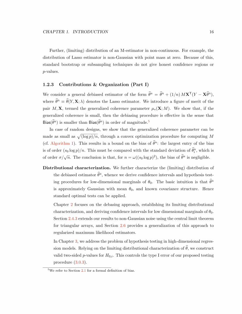
1.2.3 Contributions & Organization (Part I)
We consider a general debiased estimator of the form θu = θn + (1/n)MXT(Y − Xθn),
where θn ≡ θ(Y,X;λ) denotes the Lasso estimator. We introduce a figure of merit of the
pair M,X, termed the generalized coherence parameter µ∗(X;M). We show that, if the
generalized coherence is small, then the debiasing procedure is effective in the sense that
Bias(θu) is smaller than Bias(θn) in order of magnitude.5
In case of random designs, we show that the generalized coherence parameter can be
made as small as√
(log p)/n, through a convex optimization procedure for computing M
(cf. Algorithm 1). This results in a bound on the bias of θu: the largest entry of the bias
is of order (s0 log p)/n. This must be compared with the standard deviation of θui , which is
of order σ/√n. The conclusion is that, for n = ω((s0 log p)2), the bias of θu is negligible.
Distributional characterization. We further characterize the (limiting) distribution of
the debiased estimator θu, whence we derive confidence intervals and hypothesis test-
ing procedures for low-dimensional marginals of θ0. The basic intuition is that θu
is approximately Gaussian with mean θ0, and known covariance structure. Hence
standard optimal tests can be applied.
Chapter 2 focuses on the debasing approach, establishing its limiting distributional
characterization, and deriving confidence intervals for low dimensional marginals of θ0.
Section 2.4.3 extends our results to non-Gaussian noise using the central limit theorem
for triangular arrays, and Section 2.6 provides a generalization of this approach to
regularized maximum likelihood estimators.
In Chapter 3, we address the problem of hypothesis testing in high-dimensional regres-
sion models. Relying on the limiting distributional characterization of θ, we construct
valid two-sided p-values for H0,i. This controls the type I error of our proposed testing
procedure (3.0.3).
5We refer to Section 2.1 for a formal definition of bias.

CHAPTER 1. INTRODUCTION 17
Optimality. In Chapter 3, we prove a general lower bound on the power of our testing
procedure. Moreover, taking a minimax point of view, we prove a general upper
bound on the minimax power of tests with a given significance level α, in the case of
Gaussian random designs with i.i.d. rows. By comparing these bounds, we conclude
that the asymptotic efficiency of our approach is constant-optimal. Namely, it is lower
bounded by a constant 1/ηΣ,s0 which is bounded away from 0. Here Σ is the population
level covariance matrix of the design, i.e. Σ = E(X1XT1 ), and ηΣ,s0 is always upper
bounded by the condition number of Σ. In particular, ηI,s0 = 1. Section 3.4 contains
an overview of some of the most recent and related procedures for hypothesis testing
in high-dimensional regression, namely multisample splitting [142, 96], Ridge-type
projection estimator [16], and low dimensional projection estimator (LDPE), proposed
by [149].
Hypothesis testing under optimal sample size. In Chapter 4, we focus on Gaussian
random designs with i.i.d. rows Xi ∼ N(0,Σ). In case of Σ = I, we build upon a
rigorous characterization of the asymptotic distribution of the Lasso estimator and
its debiased version, and propose a testing procedure under the optimal sample size,
i.e. n = O(s0 log(p/s0)). For general Gaussian designs, we show that a similar distri-
butional characterization (termed ‘standard distributional limit’) can be derived from
the replica heuristics in statistical physics. This derivation suggests near-optimality
of the statistical power for a large class of Gaussian designs.
Validation. In Chapter 5, we validate our approach on both synthetic and real data, com-
paring it with other proposals. In the interest of reproducibility, an R implementation
of our algorithm is available at http://www.stanford.edu/~montanar/sslasso/.
Proofs of theorems and technical lemmas in Part I are given in Chapter 6.
1.2.4 Previously published material
The chapters of Part I are based on previous publications:
• Publication [75]: Adel Javanmard and Andrea Montanari. Confidence Intervals and
Hypothesis Testing for High-Dimensional Regression. To appear in Journal of Ma-
chine Learning Research, 2014. (Short version [71] is published in Advances in Neural
Information Processing Systems, pages 1187-1195, 2013.)

CHAPTER 1. INTRODUCTION 18
• Publication [72]: Adel Javanmard and Andrea Montanari. Hypothesis Testing in
High-Dimensional Regression under the Gaussian Random Design Model: Asymptotic
Theory. To appear in IEEE Transaction on Information Theory, 2014.
1.3 Optimal compressed sensing via spatial coupling and
approximate message passing
Compressed sensing refers to a set of techniques that recover the signal accurately from
undersampled measurements. In other words, instead of first measuring the signal and then
compressing it, these techniques aim at measuring the signal in an already compressed form
without missing any information.
Traditional sampling methods, such as Shannon-Nyquist-Whittaker, demand sampling
rate proportional to the frequency bandwidth of the signal. By contrast, compressed sensing
techniques require sampling rate proportional to the information content of the signal.
Smaller sampling rate translates to faster and cheaper data collection and processing.
The theory of compressed sensing has three key ingredients: structure of the signal,
sensing mechanism, and reconstruction algorithm. In the following, we briefly discuss these
components.
Structure of the signal: Many real world signals enjoy some types of structure. For
instance, the signal of interest belong to some known class, or it is generated according
to some known distribution. A very common structure is sparsity, meaning that most
of the information is concentrated in relatively few coordinates of the signal. More
specifically, let x ∈ Rn be an n-dimensional signal, and define its `0 norm as
‖θ‖0 = |i : θi 6= 0| ,
i.e., the number of non-zero coordinates of x. We refer to ε ≡ ‖θ‖0/n as the sparsity
level of the signal as it represents the fraction of nonzero entries. Fortunately, many
natural signals have a small sparsity level in some domain. Sparsity has long been
used by compression algorithms to decrease storage costs; the goal of sparse recovery
and compressed sensing is to exploit sparsity to decrease the required sampling rate
for exact recovery.

CHAPTER 1. INTRODUCTION 19
Sensing mechanism: The simplest way of taking measurements of signal x ∈ Rn is
through a linear operator, namely the measurements are given by
y = Ax , (1.3.1)
where A ∈ Rm×n is the measurement matrix. Of course, in most of the cases, the
measurement are contaminated by noise and hence we consider a more general model
y = Ax+ w , (1.3.2)
with w representing the noise vector. We recall that the reconstruction problem in
compressed sensing requires to reconstruct x from the measured vector y ∈ Rm, and
the measurement matrix A ∈ Rm×n.
Conventional wisdom in compressed sensing suggests that random isotropic vectors,
with small coherence number, provide a suitable class of measurement vectors. To
be more specific, in this case the sensing vectors are independently sampled from a
population F , such that F obeys the isotropy property
Eaa∗ = I , a ∼ F .
Further, the coherence parameter µ(F ) is defined to be the smallest number such that
max1≤i≤n
|ai|2 ≤ µ(F )
holds deterministically or stochastically. It turns out the smaller µ(F ), the fewer
measurements are needed for accurate recovery. Some examples are the random ma-
trices whose entries are drawn independently form Gaussian, Bernoulli, or any other
sub-gaussian distribution. Another example is obtained by sampling, uniformly at
random, form rows of the DFT matrix.
Reconstruction algorithm: Since m < n, the system of equation (1.3.1) does not, in
general, admit a unique solution. Therefore the structure of the signal must be used
as a side information in the recovery algorithm. This leads to nonlinear and more
sophisticated schemes compared to the traditional sampling theory wherein the signals
are reconstructed by applying simple linear operators.

CHAPTER 1. INTRODUCTION 20
One popular class of reconstruction schemes uses linear programming methods. Con-
sider the noiseless model (1.3.1). Among the infinitely many solutions, we are in-
terested in the sparsest one. This can be formulated as the following optimization
problem:
minimizex
‖x‖0
subject to y = Ax(1.3.3)
However, this optimization is NP-complete and cannot be used in practice. Chen et
al. [31] proposed the following convex optimization, called Basis Pursuit, as a convex
relaxation of (1.3.3).
minimizex
‖x‖1
subject to y = Ax(P1)
Clearly, this optimization can be cast as a linear programming problem. This method
is shown to be remarkably successful in recovering the signal and an elegant theory
has been developed for it [31, 30, 38, 23, 54].
There is a large corpus of research on recovering sparse signals from a few number of
measurements [36, 23, 37]. It is shown that if only k entries of x are non-vanishing, then
roughly m & 2k log(n/k) measurements are sufficient for A random, and reconstruction
can be solved efficiently by convex programming. Deterministic sensing matrices achieve
similar performance, provided they satisfy a suitable restricted isometry condition [28].
On top of this, reconstruction is robust with respect to additive noise in measurements
[24, 44], namely, under the noisy model (1.3.2) with, say, w ∈ Rm a random vector with
i.i.d. components wi ∼ N(0, σ2). In this context, the notions of ‘robustness’ or ‘stability’
refers to the existence of universal constants C such that the per-coordinate mean square
error in reconstructing x from noisy observation y is upper bounded by C σ2.
From an information-theoretic point of view it remains however unclear why we cannot
achieve the same goal with far fewer than 2 k log(n/k) measurements. Indeed, we can in-
terpret Eq. (1.3.1) as describing an analog data compression process, with y a compressed
version of x. From this point of view, we can encode all the information about x in a single
real number y ∈ R (i.e., use m = 1), because the cardinality of R is the same as the one of

CHAPTER 1. INTRODUCTION 21
Rn. Motivated by this puzzling remark, Wu and Verdu [143] introduced a Shannon-theoretic
analogue of compressed sensing, wherein the vector x has i.i.d. components xi ∼ pX . Cru-
cially, the distribution pX is available to, and may be used by the reconstruction algorithm.
Under the mild assumptions that sensing is linear (as per (1.3.1)), and that the recon-
struction mapping is Lipschitz continuous, they proved that compression is asymptotically
lossless if and only if
m ≥ nd(pX) + o(n) . (1.3.4)
Here d(pX) is the (upper) Renyi information dimension of the distribution pX . We refer to
Section 7.1 for a precise definition of this quantity. Suffices to say that, if pX is ε-sparse
(i.e., if it puts mass at most ε on nonzeros) then d(pX) ≤ ε. Also, if pX is the convex
combination of a discrete part (sum of Dirac’s delta) and an absolutely continuous part
(with a density), then d(pX) is equal to the weight of the absolutely continuous part.
This result is quite striking. For instance, it implies that, for random k-sparse vectors,
m ≥ k + o(n) measurements are sufficient. Also, if the entries of x are random and take
values in, say, −10,−9, . . . ,−9,+10, then a sublinear number of measurements m =
o(n), is sufficient! At the same time, the result of Wu and Verdu presents two important
limitations. First, it does not provide robustness guarantees of the type described above.
Second and most importantly, it does not provide any computationally practical algorithm
for reconstructing x from measurements y.
In an independent line of work, Krzakala et al. [82] developed an approach that leverages
on the idea of spatial coupling. This idea was introduced in the compressed sensing literature
by Kudekar and Pfister [84] (see [85] and Section 7.3 for a discussion of earlier work on
this topic). Spatially coupled matrices are, roughly speaking, random sensing matrices
with a band-diagonal structure. The analogy is, this time, with channel coding.6 In this
context, spatial coupling, in conjunction with message-passing decoding, allows to achieve
Shannon capacity on memoryless communication channels. It is therefore natural to ask
whether an approach based on spatial coupling can enable to sense random vectors x at
an undersampling rate m/n close to the Renyi information dimension of the coordinates of
x, d(pX). Indeed, the authors of [82] evaluate such a scheme numerically on a few classes
of random vectors and demonstrate that it indeed achieves rates close to the fraction of
6Unlike [82], we follow here the terminology developed within coding theory.

CHAPTER 1. INTRODUCTION 22
non-zero entries. They also support this claim by insightful statistical physics arguments.
In PartII of this dissertation, we fill the gap between the above works, and present the
following contributions:
Construction. We describe a construction for spatially coupled sensing matrices A that is
somewhat broader than the one of [82] and give precise prescriptions for the asymp-
totic values of various parameters. We also use a somewhat different reconstruc-
tion algorithm from the one in [82], by building on the approximate message passing
(AMP) approach of [42, 43]. AMP algorithms have the advantage of smaller memory
complexity with respect to standard message passing, and of smaller computational
complexity whenever fast multiplication procedures are available for A.
Rigorous proof of convergence. Our main contribution is a rigorous proof that the
above approach indeed achieves the information-theoretic limits set out by Wu and
Verdu [143]. Indeed, we prove that, for sequences of spatially coupled sensing matrices
A(n)n∈N, A(n) ∈ Rm(n)×n with asymptotic undersampling rate δ = limn→∞m(n)/n,
AMP reconstruction is with high probability successful in recovering the signal x, pro-
vided δ > d(pX).
Robustness to noise. We prove that the present approach is robust7 to noise in the fol-
lowing sense. For any signal distribution pX and undersampling rate δ, there exists a
constant C such that the output x(y) of the reconstruction algorithm achieves a mean
square error per coordinate n−1E‖x(y) − x‖22 ≤ C σ2. This result holds under the
noisy measurement model (1.3.2) for a broad class of noise models for w, including
i.i.d. noise coordinates wi with Ew2i = σ2 <∞.
Non-random signals. Our proof does not apply uniquely to random signals x with i.i.d.
components, but indeed to more general sequences of signals x(n)n∈N, x(n) ∈ Rn
indexed by their dimension n. The conditions required are: (1) that the empirical
distribution of the coordinates of x(n) converges (weakly) to pX ; and (2) that ‖x(n)‖22converges to the second moment of the asymptotic law pX .
There is a fundamental reason why this more general framework turns out to be
equivalent to the random signal model. This can be traced back to the fact that, within
7This robustness bound holds for all δ > D(pX), where D(pX) is the upper MMSE dimension of pX .(see Definition 7.1.4). It is worth noting that D(pX) = d(pX) for a broad class of distributions pX includingdistributions without singular continuous component.

CHAPTER 1. INTRODUCTION 23
Classical Compressed Sensing Our Approach
Structure Sparsity Information dimension
Rate m = Ck log(n/k) m = d(pX) · n
Measurements Random isotropic vectors Spatially coupled matrices
Reconstruction Convex optimization Bayesian AMP
Robustness MSE ≤ Cσ2 MSE ≤ C(x)σ2
Table 1.3.1 Comparison between classical approach to compressed sensing and our approach.
our construction, the columns of the matrix A are probabilistically exchangeable.
Hence any vector x(n) is equivalent to the one whose coordinates have been randomly
permuted. The latter is in turn very close to the i.i.d. model. By the same token, the
rows of A are exchangeable and hence the noise vector w does not need to be random
either.
Interestingly, the present framework changes the notion of ‘structure’ that is relevant for
reconstructing the signal x. Indeed, the focus is shifted from the sparsity of x to the in-
formation dimension d(pX). In other words, the signal structure that facilitates recovery
from a small number of linear measurements is the low-dimensional structure in an infor-
mation theoretic sense, quantified by the information dimension of the signal. Table 1.3.1
provides a comparison between pillars of traditional compressed sensing and principles of
our approach. We refer to Part II for a detailed discussion on the salient features of our
approach presented in Table 1.3.1.
1.3.1 A toy example
The following example demonstrates the dramatic improvement achieved by our scheme.
Consider a signal x ∈ Rn whose coordinates are generated i.i.d. from the distribution
pX = 0.2δ0 + 0.3δ1 + 0.2δ−1 + 0.2δ3 + 0.1Uniform(−2, 2). Further suppose that we take
m noiseless linear measurements of x. Classical scheme based on `1 minimization (P1)
require m ≥ 0.97n for exact recovery. More generally, Donoho and Tanner [34] showed that
the reconstruction algorithm (P1) undergoes a phase transition: they characterized a curve
ε→ δ`1(ε) in the (ε, δ) plane such that the following happens for sensing matrices A ∈ Rm×n
CHAPTER 1. INTRODUCTION 24
δ`1(ε)
ε
δ
(0.8, 0.97)
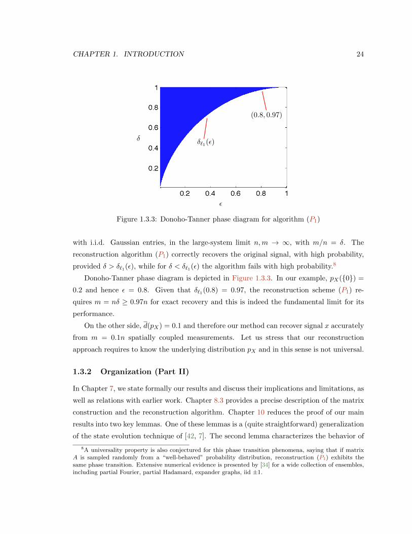
Figure 1.3.3: Donoho-Tanner phase diagram for algorithm (P1)
with i.i.d. Gaussian entries, in the large-system limit n,m → ∞, with m/n = δ. The
reconstruction algorithm (P1) correctly recovers the original signal, with high probability,
provided δ > δ`1(ε), while for δ < δ`1(ε) the algorithm fails with high probability.8
Donoho-Tanner phase diagram is depicted in Figure 1.3.3. In our example, pX(0) =
0.2 and hence ε = 0.8. Given that δ`1(0.8) = 0.97, the reconstruction scheme (P1) re-
quires m = nδ ≥ 0.97n for exact recovery and this is indeed the fundamental limit for its
performance.
On the other side, d(pX) = 0.1 and therefore our method can recover signal x accurately
from m = 0.1n spatially coupled measurements. Let us stress that our reconstruction
approach requires to know the underlying distribution pX and in this sense is not universal.
1.3.2 Organization (Part II)
In Chapter 7, we state formally our results and discuss their implications and limitations, as
well as relations with earlier work. Chapter 8.3 provides a precise description of the matrix
construction and the reconstruction algorithm. Chapter 10 reduces the proof of our main
results into two key lemmas. One of these lemmas is a (quite straightforward) generalization
of the state evolution technique of [42, 7]. The second lemma characterizes the behavior of
8A universality property is also conjectured for this phase transition phenomena, saying that if matrixA is sampled randomly from a “well-behaved” probability distribution, reconstruction (P1) exhibits thesame phase transition. Extensive numerical evidence is presented by [34] for a wide collection of ensembles,including partial Fourier, partial Hadamard, expander graphs, iid ±1.

CHAPTER 1. INTRODUCTION 25
the state evolution recursion, and is proved in Chapter 11. In Chapter 12, we study the
problem of sampling a random signal with sparse support in frequency domain, and propose
a sampling scheme inspired by the idea of spatial coupling. As we discuss one possible
implementation of this idea is through Gabor transform. We show empirically that this
scheme achieves correct reconstruction at information-theoretically optimal undersampling
rate.
The proof of a number of intermediate technical steps is deferred to the appendices.
1.3.3 Previously published material
The chapters of Part II are based on previous publications:
• Publication [41]: David L. Donoho, Adel Javanmard and Andrea Montanari. Information-
Theoretically Optimal Compressed Sensing via Spatial Coupling and Approximate
Message Passing. IEEE Transactions on Information Theory, 59(11):7434-7464, 2013.
(Short version [40] is published in IEEE International Symposium on Information
Theory (ISIT), pages 1231-1235, 2012.)
• Publication [70]: Adel Javanmard and Andrea Montanari. Subsampling at Informa-
tion Theoretically Optimal Rates. In IEEE International Symposium on Information
Theory (ISIT), pages 2431-2435, 2012.
• Publication [74]: Adel Javanmard and Andrea Montanari. State Evolution for General
Approximate Message Passing Algorithms, with Applications to Spatial Coupling.
Journal of Information and Inference, 2(2):115-144, 2013.

Part I
Assigning Statistical Significance in
High-Dimensional Problems
26

Chapter 2
Confidence Intervals for
High-Dimensional Models
We recall the linear regression model with n i.i.d. samples and p parameters, as described
by (1.1.6), where the goal is to learn vector of parameters θ0.
In the classic setting, n p and the estimation method of choice is ordinary least
squares yielding θOLS = (XTX)−1XTY . Least squares θOLS has an explicit formulation,
and admits an exact distributional characterization. In particular θOLS is Gaussian with
mean θ0 and covariance σ2(XTX)−1. This directly allows to construct confidence intervals
for single parameters θ0,i based on the estimate θOLS.1
In the high-dimensional setting where p > n, the matrix (XTX) is rank deficient and
one has to resort to structured estimators. We discussed some remarkable properties of
these estimator in the introduction. These properties, however, come at a price. Deriving
an exact characterization for the distribution of structured estimators is not tractable in
general, and hence there is no simple procedure to construct confidence intervals and p-
values. A closely related property is that structured estimators are biased, an unavoidable
property in high dimension, since a point estimate in p-dimension must be produced from
data in lower dimension Y ∈ Rn, n < p.
In our presentation, we focus on Lasso estimator θn ≡ θn(Y,X;λ), as per (1.1.7) which
promotes sparse reconstructions through an `1 penalty. Later in the chapter, we discuss the
case of general structured estimators.
1For instance, letting Q ≡ (XTX/n)−1, θOLSi − 1.96σ
√Qii/n, θ
OLSi + 1.96σ
√Qii/n] is a 95% confidence
interval [141].
27

CHAPTER 2. CONFIDENCE INTERVALS FOR HIGH-DIMENSIONAL MODELS 28
2.1 Preliminaries and notations
In this section we introduce some basic definitions used throughout this part, starting with
simple notations.
For a matrix A and set of indices I, J , we let AI,J denote the submatrix formed by the
rows in I and columns in J . Also, AI,· (resp. A·,I) denotes the submatrix containing just
the rows (reps. columns) in I. Likewise, for a vector v, vI is the restriction of v to indices
in I. We use the shorthand A−1I,J = (A−1)I,J . In particular, A−1
i,i = (A−1)i,i. The maximum
and the minimum singular values of A are respectively denoted by σmax(A) and σmin(A).
We write ‖v‖p for the standard `p norm of a vector v, i.e., ‖v‖p = (∑
i |vi|p)1/p. and ‖v‖0for the number of nonzero entries of v. For a matrix A, ‖A‖p is the `p operator norm, and
|A|p is the elementwise `p norm. For a vector v, supp(v) represents the positions of nonzero
entries of v. Throughout, φ(x) = e−x2/2/√
2π, and Φ(x) ≡∫ x−∞ φ(t)dt respectively denote
the PDF and the CDF of the standard normal distribution. Finally, with high probability
(w.h.p) means with probability converging to one as n→∞.
We let Σ ≡ XTX/n be the sample covariance matrix. For p > n, Σ is always singular.
However, we may require Σ to be nonsingular for a restricted set of directions.
Definition 2.1.1. Given a symmetric matrix Σ ∈ Rp×p and a set S ⊆ [p], the corresponding
compatibility constant is defined as
φ2(Σ, S) ≡ minθ∈Rp
|S| 〈θ, Σ θ〉‖θS‖21
: θ ∈ Rp, ‖θSc‖1 ≤ 3‖θS‖1. (2.1.1)
We say that Σ ∈ Rp×p satisfies the compatibility condition for the set S ⊆ [p], with constant
φ0 if φ(Σ, S) ≥ φ0. We say that it holds for the design matrix X, if it holds for Σ = XTX/n.
In the following, we shall drop the argument Σ if clear from the context. Note that
a slightly more general definition is used normally [19, Section 6.13], where the condition
‖θSc‖1 ≤ 3‖θS‖1, is replaced by ‖θSc‖1 ≤ L‖θS‖1. The resulting constant φ(Σ, S, L) depends
on L. For the sake of simplicity, we restrict ourselves to the case L = 3.
Definition 2.1.2. The sub-gaussian norm of a random variable X, denoted by ‖X‖ψ2, is
defined as
‖X‖ψ2 = supq≥1
q−1/2(E|X|q)1/q .

CHAPTER 2. CONFIDENCE INTERVALS FOR HIGH-DIMENSIONAL MODELS 29
For a random vector X ∈ Rn, its sub-gaussian norm is defined as
‖X‖ψ2 = supx∈Sn−1
‖〈X,x〉‖ψ2 ,
where Sn−1 denotes the unit sphere in Rn.
Definition 2.1.3. The sub-exponential norm of a random variable X, denoted by ‖X‖ψ1,
is defined as
‖X‖ψ1 = supq≥1
q−1(E|X|q)1/q .
For a random vector X ∈ Rn, its sub-exponential norm is defined as
‖X‖ψ1 = supx∈Sn−1
‖〈X,x〉‖ψ1 ,
where Sn−1 denotes the unit sphere in Rn.
We next formally define bias of an estimator.
Definition 2.1.4. Given an estimator θn of the parameter vector θ0, we define its bias to
be the vector
Bias(θn) ≡ Eθn − θ0|X . (2.1.2)
Note that, if the design is random, Bias(θn) is a measurable function of X. If the de-
sign is deterministic, Bias(θn) is a deterministic quantity as well, and the conditioning is
superfluous.
Throughout, we denote by S ≡ supp(θ0) the support of θ0 ∈ Rp, defined as
supp(θ0) ≡ i ∈ [p] : θ0,i 6= 0 ,
where we use the notation [p] = 1, . . . , p. We further let s0 ≡ |S|.
2.2 The bias of the Lasso
Structured estimators are biased due to the regularization term. In particular, Lasso esti-
mator is biased towards small `1 norm.

CHAPTER 2. CONFIDENCE INTERVALS FOR HIGH-DIMENSIONAL MODELS 30
Let us begin with the simple case of X = I, n = p. The observed samples are given by
Y = θ0 + W . In this case, Lasso estimator is given by the soft thresholding function, i.e.,
θn = η(Y ;λ), where η : R× R+ → R is defined as
η(y;λ) =
y − λ if y > λ,
0 if − λ ≤ y ≤ λ,
y + λ otherwise.
(2.2.1)
and for a vector u ∈ Rn, we let η(u) denote the vector (η(u1), · · · , η(un)) obtained by
applying η component-wise. By a simple algebraic manipulation, we have
Bias(θni ) = −λ+ (λ− θ0,i)Φ(λ− θ0,i) + (λ+ θ0,i)Φ(−λ− θ0,i) + φ(λ− θ0,i)− φ(−λ− θ0,i).
Clearly, by choosing θ0,i large enough, Bias(θni ) and therefore ‖Bias(θn)‖∞ will be larger
than cλ for any fixed 0 < c < 1. Following theorem lower bounds the bias of the Lasso for
a broad class of design matrices.
Theorem 2.2.1. Consider linear model (1.1.6) and suppose that X has independent sub-
gaussian rows, with mean zero and subgaussian norm ‖X1‖ψ2 = κ, for some constant
κ ∈ (0,∞). Let θn be the Lasso estimator, with λ = cσ√
(log p)/n. Then, there exist
positive constants c∗, c∗∗ such that if n ≥ (3c∗∗s0/c)2 log p and p ≥ 1348/(c2−48), then the
following holds true: there exist a set of design matrices Bn ⊆ Rn×p, and coefficient vectors
θ0 ∈ Rp, ‖θ0‖0 ≤ s0, such that
X ∈ Bn ⇒ ‖Bias(θn)‖∞ ≥λ
3=cσ
3
√log p
n, (2.2.2)
P(Bn) ≥ 1− 4 e−c1n − 2 p−3 , (2.2.3)
where c1 = 1/(4c∗κ4).
A formal proof of this theorem is given in Section 6.1.4.
Bias of the Lasso estimator is a major difficulty in achieving our goal, namely construct-
ing confidence intervals for single parameters θ0,i. To overcome this challenge, we construct
a debiased estimator θu from the Lasso solution, and characterize its limiting distribution.
Armed with such characterization, we construct confidence intervals for the true parameters.

CHAPTER 2. CONFIDENCE INTERVALS FOR HIGH-DIMENSIONAL MODELS 31
2.3 Compensating the bias of the Lasso
In this section we present our construction of a debiased estimator θu and compare its bias
with the bias of the Lasso estimator.
2.3.1 A debiased estimator for θ0
We begin with the classical case n > p. Here, the least squares estimator is given by
θOLS = (Σ−1XTY/n), where Σ ≡ (XXT/n) denotes the sample covariance. Further, θOLS
is unbiased estimator for θ0.
In the high-dimensional regime, however, Σ is not invertible since n < p and therefore
θOLS cannot even be defined. Instead, we define a similar estimator θ, using a matrix
M ∈ Rp×p in lieu of Σ−1. (Take M to be an arbitrary matrix for now. We will discuss a
specific choice of M later.)
Define
θ ≡ 1
nMXTY . (2.3.1)
Plugging Y = Xθ0 +W in (2.3.1), we get
θ =1
nMXTXθ0 +
1
nMXTW
= θ0 + (M Σ− I)θ0︸ ︷︷ ︸Bias
+1
nMXTW︸ ︷︷ ︸
zero-mean noise
.
Note that Bias(θ) depends on the unknown vector of parameters θ0. In order to debias the
estimator, we use Lasso solution θn as an estimate of θ0. This leads us to a new estimator
θ∗ defined as follows.
θ∗(Y,X;M,λ) ≡ θ − (M Σ− I)θn(λ)
=1
nMXTY − (M Σ− I)θn(λ)
= θn(λ) +1
nMXT(Y −Xθn(λ)) . (2.3.2)
For notational simplicity, we shall omit the arguments Y,X,M, λ unless they are required
for clarity.

CHAPTER 2. CONFIDENCE INTERVALS FOR HIGH-DIMENSIONAL MODELS 32
2.3.1.1 How to choose M?
The quality of this debiasing procedure depends of course on the choice of M , as well as on
the design X. We characterize the pair (X,M) by the following figure of merit.
Definition 2.3.1. Given the pair X ∈ Rn×p and M ∈ Rp×p, let Σ = XTX/n denote the
associated sample covariance. Then, the generalized coherence parameter of X,M , denoted
by µ∗(X;M), is
µ∗(X;M) ≡∣∣M Σ− I
∣∣∞ . (2.3.3)
Here and below | · |∞ denotes the entrywise `∞ norm. The minimum (generalized) coher-
ence of X is µmin(X) = minM∈Rp×p µ∗(X;M). We denote by Mmin(X) any minimizer of
µ∗(X;M).
Note that the minimum coherence can be computed efficiently since M 7→ µ∗(X;M) is
a convex function (even more, the optimization problem is a linear program).
The motivation for our terminology can be grasped by considering the following special
case.
Remark 2.3.2. Assume that the columns of X are normalized to have `2 norm equal to√n
(i.e. ‖Xei‖2 =√n for all i ∈ [p]), and M = I. Then (M Σ − I)i,i = 0, and the maximum
|M Σ − I|∞ = maxi 6=j |(Σ)ij |. In other words µ(X; I) is the maximum normalized scalar
product between distinct columns of X:
µ∗(X; I) =1
nmaxi 6=j
∣∣〈Xei,Xej〉∣∣ . (2.3.4)
The quantity (2.3.4) is known as the coherence parameter of the matrix X/√n and
was first defined in the context of approximation theory by Mallat and Zhang [92], and by
Donoho and Huo [39].
Assuming, for simplicity, that the columns of X are normalized so that ‖Xei‖2 =√n, a
small value of the coherence parameter µ∗(X; I) means that the columns of X are roughly
orthogonal. We emphasize however that µ∗(X;M) can be much smaller than its classi-
cal coherence parameter µ∗(X; I). For instance, µ∗(X; I) = 0 if and only if X/√n is an
orthogonal matrix. On the other hand, µmin(X) = 0 if and only if X has rank p.2
2Of course this example requires n ≥ p. It is the simplest example that illustrates the difference betweencoherence and generalized coherence, and it is not hard to find related examples with n < p.

CHAPTER 2. CONFIDENCE INTERVALS FOR HIGH-DIMENSIONAL MODELS 33
The following theorem is a slight generalization of a result of [134] and its proof is given
in Section 6.1.1. Let us emphasize that it applies to deterministic design matrices X.
Theorem 2.3.3. Let X ∈ Rn×p be any (deterministic) design matrix, and θ∗ = θ∗(Y,X;M,λ)
be a general debiased estimator as per Eq. (2.3.2). Then, setting Z = MXTW/√n, we have
√n(θ∗ − θ0) = Z + ∆ , Z ∼ N(0, σ2M ΣMT) , ∆ =
√n(M Σ− I)(θ0 − θn) . (2.3.5)
Further, assume that X satisfies the compatibility condition for the set S = supp(θ0), |S| ≤s0, with constant φ0, and has generalized coherence parameter µ∗ = µ∗(X;M), and let
K ≡ maxi∈[p] Σi,i. Then, letting λ = σ√
(c2 log p)/n, we have
P(‖∆‖∞ ≥
4cµ∗σs0
φ20
√log p
)≤ 2p−c0 , c0 =
c2
32K− 1 . (2.3.6)
Further, if M = Mmin(X) minimizes the convex cost function |M Σ − I|∞, then µ∗ can be
replaced by µmin(X) in Eq. (2.3.6).
The above theorem decomposes the estimation error (θ∗−θ0) into a zero mean Gaussian
term Z/√n and a bias term ∆/
√n whose maximum entry is bounded as per Eq. (2.3.6).
This estimate on ‖∆‖∞ depends on the design matrix through two constants: the com-
patibility constant φ0 and the generalized coherence parameter µ∗(X;M). The former is
a well studied property of the design matrix [19, 133], and assuming φ0 of order one is
nearly necessary for the Lasso to achieve optimal estimation rate in high dimension. On
the contrary, the definition of µ∗(X;M) is a new contribution of the present work.
The next theorem establishes that, for a natural probabilistic model of the design matrix
X, both φ0 and µ∗(X;M) can be bounded with probability converging rapidly to one as
n, p→∞.
Theorem 2.3.4. Let Σ ∈ Rp×p be such that σmin(Σ) ≥ Cmin > 0, and σmax(Σ) ≤ Cmax <
∞, and maxi∈[p] Σii ≤ 1. Assume XΣ−1/2 to have independent subgaussian rows, with zero
mean and subgaussian norm ‖Σ−1/2X1‖ψ2 = κ, for some constant κ ∈ (0,∞).
(a) For φ0, s0,K ∈ R>0, let En = En(φ0, s0,K) be the event that the compatibility condition
holds for Σ = (XTX/n), for all sets S ⊆ [p], |S| ≤ s0 with constant φ0 > 0, and that

CHAPTER 2. CONFIDENCE INTERVALS FOR HIGH-DIMENSIONAL MODELS 34
maxi∈[p] Σi,i ≤ K. Explicitly
En(φ0, s0,K) ≡
X ∈ Rn×p : minS: |S|≤s0
φ(Σ, S) ≥ φ0, maxi∈[p]
Σi,i ≤ K, Σ = (XTX/n).
(2.3.7)
Then there exists c∗ ≤ 2000 such that the following happens. If n ≥ ν0 s0 log(p/s0),
ν0 ≡ 5× 10⁴c∗(Cmax/Cmin)2κ4, φ0 =√Cmin/2, and K ≥ 1 + 20κ2
√(log p)/n, then
P(X ∈ En(φ0, s0,K)
)≥ 1− 4 e−c1n , c1 ≡
1
4c∗κ4. (2.3.8)
(b) For a > 0, let Gn = Gn(a) be the following event:
Gn(a) ≡
X ∈ Rn×p : µmin(X) < a
√log p
n
. (2.3.9)
Then, for n ≥ a2Cmin log p/(4e2Cmaxκ4)
P(X ∈ Gn(a)
)≥ 1− 2 p−c2 , c2 ≡
a2Cmin
24e2κ4Cmax− 2 . (2.3.10)
The proof of this theorem is given in Section 6.1.2 (for part (a)) and Section 6.1.3 (part
(b)).
The proof that event En holds with high probability relies crucially on a theorem by
Rudelson and Zhou [116, Theorem 6]. Simplifying somewhat, the latter states that, if the
restricted eigenvalue condition of [14] holds for the population covariance Σ, then it holds
with high probability for the sample covariance Σ. (Recall that the restricted eigenvalue
condition is implied by a lower bound on the minimum singular value3, and that it implies
the compatibility condition [133].)
Motivated by Theorem 2.3.3, we propose a procedure for constructing matrix M . Our
approach is to construct M by solving a convex program that aims at optimizing two objec-
tives. One one hand, we try to control |M Σ−I|∞ which, as shown in Theorem 2.3.3, controls
the non-Gaussianity and bias of the estimator. On the other, we minimize [M ΣM ]i,i, for
each i ∈ [p], which controls the variance of of the i-th coordinate of the estimator. The pro-
cedure and the corresponding debiased estimator θu are described in Algorithm 1. Note that
3Note, in particular, at the cost of further complicating the last statement, the condition σmin(Σ) = Ω(1)can be further weakened.

CHAPTER 2. CONFIDENCE INTERVALS FOR HIGH-DIMENSIONAL MODELS 35
Algorithm 1 Unbiased estimator for θ0 in high-dimensional linear regression models
Input: Measurement vector Y , design matrix X, parameters λ, µ.Output: Unbiased estimator θu.
1: Let θn = θn(Y,X;λ) be the Lasso estimator as per Eq. (1.1.7).2: Set Σ ≡ (XTX)/n.3: for i = 1, 2, . . . , p do4: Let mi be a solution of the convex program:
minimize mTΣm
subject to ‖Σm− ei‖∞ ≤ µ ,(2.3.11)
where ei ∈ Rp is the vector with one at the i-th position and zero everywhere else.5: Set M = (m1, . . . ,mp)
T. If any of the above problems is not feasible, then set M = Ip×p.
6: Define the estimator θu as follows:
θu = θn(λ) +1
nMXT(Y −Xθn(λ)) (2.3.12)
event Gn, defined by (2.3.9), can be equivalently stated as the event that problem (2.3.11),
for all i ∈ [p], is feasible with µ = a√
(log p)/n.
Finally, by putting together Theorem 2.3.3 and Theorem 2.3.4, we obtain the following
conclusion. We refer to Section 6.1.5 for the proof of Theorem 2.3.5.
Theorem 2.3.5. Consider the linear model (1.1.6) and let θu be defined as per Eq. (2.3.12)
in Algorithm 1, with µ = a√
(log p)/n. Then, setting Z = MXTW/√n, we have
√n(θu − θ0) = Z + ∆ , Z|X ∼ N(0, σ2M ΣMT) , ∆ =
√n(M Σ− I)(θ0 − θn) . (2.3.13)
Further, under the assumptions of Theorem 2.3.4, and for n ≥ max(ν0s0 log(p/s0), ν1 log p),
ν1 = max(1600κ4, a2/(4e2κ4)), and λ = σ√
(c2 log p)/n, we have
P‖∆‖∞ ≥
(16ac σ
Cmin
)s0 log p√n
≤ 4 e−c1n + 4 p−c0∧c2 . (2.3.14)
where c0 = (c2/48)− 1 and c1, c2 are given by Eqs. (2.3.8) and (2.3.10).
Finally, the tail bound (2.3.14) holds for any choice of M that is only function of the
design matrix X, and satisfies the feasibility condition in Eq. (2.3.11), i.e. |M Σ− I|∞ ≤ µ.
Assuming σ,Cmin of order one, the last theorem establishes that, for random designs,

CHAPTER 2. CONFIDENCE INTERVALS FOR HIGH-DIMENSIONAL MODELS 36
the maximum size of the ‘bias term’ ∆i over i ∈ [p] is:
‖∆‖∞ = O(s0 log p√
n
)(2.3.15)
On the other hand, the ‘noise term’ Zi is roughly of order
√[M ΣMT]ii. Bounds on the
variances [M ΣMT]ii will be given in next Chapter (cf. Eq. (6.2.1) in the Proof of The-
orem 3.1.1) showing that, if M is computed through Algorithm 1, [M ΣMT]ii is of order
one for a broad family of random designs. As a consequence |∆i| is much smaller than |Zi|whenever s0 = o(
√n/ log p). We summarize these remarks below.
Remark 2.3.6. Theorem 2.3.5 only requires that the support size satisfies s0 = O(n/ log p).
If we further assume s0 = o(√n/ log p), then we have ‖∆‖∞ = o(1) with high probability.
Hence, θu is an asymptotically unbiased estimator for θ0.
A more formal comparison of the bias of θu, and of the one of the Lasso estimator θn can
be found in Section 2.3.2 below. Section 2.3.3 compares our approach with other related
work.
As it can be seen from the statement of Theorem 2.3.3 and Theorem 2.3.4, the claim
of Theorem 2.3.5 does not rely on the specific choice of the objective function in opti-
mization problem (2.3.11) and only uses the constraint on ‖Σm − ei‖∞. In particular it
holds for any matrix M that is feasible. On the other hand, the specific objective function
problem (2.3.11) minimizes the variance of the noise term, Var(Zi).
2.3.2 Discussion: bias reduction
Theorems 2.3.3 and 2.3.4 provide a quantitative framework to discuss in what sense the
Lasso estimator θn is asymptotically biased, while the debiased estimator θu is asymptoti-
cally unbiased.
Invoking definition of bias (2.1.2), it follows from Eq. (2.3.5) that
Bias(θu) =1√nE∆|X . (2.3.16)
Applying Theorem 2.3.5 with high probability, ‖∆‖∞ = O(s0 log p/√n). The next corollary
states that this bound on ‖∆‖∞ translates into a bound on Bias(θu) for all X in a set that
has probability rapidly converging to one as n, p get large.

CHAPTER 2. CONFIDENCE INTERVALS FOR HIGH-DIMENSIONAL MODELS 37
Corollary 2.3.7. Under the assumptions of Theorem 2.3.5, let c1, c2 be defined as per
equations (2.3.8) and (2.3.10). Then we have
X ∈ En(√Cmin/2, s0, 3/2) ∩ Gn(a) ⇒ ‖Bias(θu)‖∞ ≤
160a
Cmin· σs0 log p
n, (2.3.17)
P(X ∈ En(
√Cmin/2, s0, 3/2) ∩ Gn(a)
)≥ 1− 4e−c1n − 2 p−c2 . (2.3.18)
The proof of this corollary can be found in Section 6.1.6.
This result can be contrasted with a converse result for the Lasso estimator. Namely, as
stated in Theorem 2.2.1, there are choices of the vector θ0, and of the design covariance Σ,
such that ‖Bias(θn)‖∞ is of order σ√
(log p)/n. Comparing this bound with the bound on
‖Bias(θu)‖∞, as established in Corollary 2.3.7, we conclude that if s0 is significantly smaller
than√n/ log p (which is the main regime studied in this chapter), then ‖Bias(θn)‖∞
‖Bias(θu)‖∞. Hence, our approach has effectively reduced the bias.
2.3.3 Comparison with earlier results
The idea of constructing a debiased estimator of the form θu = θn + (1/n)MXT(Y −Xθn)
was used by Javanmard and Montanari in [72], that suggested the choice M = cΣ−1, with
Σ = E(X1XT1 ) the population covariance matrix and c a positive constant. We discuss this
approach meticulously in Chapter 4. Van de Geer, Buhlmann, Ritov and Dezeure [134] used
the same construction with M an estimate of Σ−1 which is appropriate for sparse inverse
covariances. These authors prove semi-parametric optimality in a non-asymptotic setting,
provided the sample size is at least n = Ω((s0 log p)2).
The rationale for choosing M to be an estimate of Σ−1 is as follows.
One step of Newton method. Recall that Lasso estimator is given as the solution of
the optimization problem below:
θn ≡ argminθ∈Rp
1
2n‖Y −Xθ‖2 + λ‖θ‖1
.
Lasso solution θn is biased due to the regularization term. On the other hand, it is easy to
see that
argminθ∈Rp
1
2nE(‖Y −Xθ‖2) = θ0 , (2.3.19)

CHAPTER 2. CONFIDENCE INTERVALS FOR HIGH-DIMENSIONAL MODELS 38
where the expectation is taken with respect to the law of the samples (Yi, Xi)ni=1. There-
fore, a natural approach for debiasing is to take θn as the initial guess and perform one step
of Newton method to move towards the minimizer of (2.3.19), i.e., θ0. This leads to
θ∗(Y,X; Σ−1, λ) = θn +1
nΣ−1XT(Y −Xθn) .
This justifies the choice of M = Σ−1.
From a technical point of view, the presented approach in this chapter starts from a
simple decomposition of the debiased estimator θu into a Gaussian part and an error term,
already used in [134]. However, departing radically from earlier work, we realize that M
need not be a good estimator of Σ−1 in order for the debiasing procedure to work. We
instead set M as to minimize the error term and the variance of the Gaussian term. As
a consequence of this choice, our approach applies to general covariance structures Σ. By
contrast, earlier approaches applied only to sparse Σ, as in [72], or sparse Σ−1 as in [134].
The only assumptions we make on Σ are the standard compatibility conditions required for
high-dimensional consistency [19].
In the case of linear statistical models considered here, the authors of [134] construct
a debiased estimator of the form (2.3.2). However, instead of solving the optimization
problem (2.3.11), they follow [149] and use the regression coefficients of the i-th column of
X on the other columns to construct the i-th row of M . These regression coefficients are
computed, once again, using the Lasso (node-wise Lasso). It useful to spell out the most
important differences between our contribution and the ones of [134]:
1. The case of fixed non-random designs is covered by [134, Theorem 2.1], which should
be compared to our Theorem 2.3.3. While in our case the bias is controlled by the
generalized coherence parameter, a similar role is played in [134] by the regularization
parameters of the nodewise Lasso.
2. The case of random designs is covered by [134, Theorem 2.2, Theorem 2.4], which
should be compared with our Theorem 2.3.5. In this case, the assumptions underlying
our result are less restrictive. More precisely:
(a) [134, Theorem 2.2, Theorem 2.4] assume X has i.i.d. rows, while we only assume
the rows are independent.
(b) [134, Theorem 2.2, Theorem 2.4] assumes the rows of the inverse covariance

CHAPTER 2. CONFIDENCE INTERVALS FOR HIGH-DIMENSIONAL MODELS 39
matrix Σ−1 are sparse. More precisely, letting sj be the number of non-zero
entries of the j-th row of Σ−1, [134] assumes maxj∈[p] sj = o(n/ log p), that is
much smaller than p. We do not make any sparsity assumption on Σ−1, and sj
can be as large as p. [134, Theorem 2.4] also considers a slightly different setting,
where X has bounded entries, under analogous sparsity assumptions.
It is currently unknown whether the sparsity assumption in [134] is required for that
approach to work, or it is rather an artifact of the specific analysis. Indeed [134,
Theorem 2.1] can in principle be used to weaken this condition.
In addition, our Theorem 2.3.5 provides the specific dependence on the maximum and
minimum singular value of Σ.
Note that solving the convex problem (2.3.11) is not more burdensome than solving
the nodewise Lasso as in [149, 134], This can be confirmed by checking that the dual of
problem (2.3.11) is an `1-regularized quadratic optimization problem. It has therefore the
same complexity as the nodewise Lasso (but it is different from the nodewise Lasso). We
refer to Section 5.1 for a thorough discussion on this.
2.4 Confidence intervals
A direct application of Theorem 2.3.5 is to derive confidence intervals for each single pa-
rameter θ0,i of a high-dimensional model. Throughout, we make the sparsity assumption
s0 = o(√n/ log p) and omit explicit constants that can be readily derived from Theorem
2.3.5.
2.4.1 Preliminary lemmas
As discussed above, the bias term ∆ is negligible with respect to the random term Z in
the decomposition (2.3.13), provided the latter has variance of order one. Our first lemma
establishes that this is indeed the case.
Lemma 2.4.1. Let M = (m1, . . . ,mp)T be the matrix with rows mT
i obtained by solving
convex program (2.3.11) in Algorithm 1. Then for all i ∈ [p],
[M ΣMT]i,i ≥(1− µ)2
Σi,i
.

CHAPTER 2. CONFIDENCE INTERVALS FOR HIGH-DIMENSIONAL MODELS 40
Lemma 2.4.1 is proved in Appendix A.1.
Using this fact, we can then characterize the asymptotic distribution of the residu-
als (θu − θ0,i). Theorem 2.3.5 naturally suggests to consider the scaled residual√n(θui −
θ0,i)/(σ[M ΣMT]1/2i,i ). In the next lemma we consider a slightly more general scaling, replac-
ing σ by a consistent estimator σ.
Lemma 2.4.2. Consider a sequence of design matrices X ∈ Rn×p, with dimensions n→∞,
p = p(n) → ∞ satisfying the following assumptions, for constants Cmin, Cmax, κ ∈ (0,∞)
independent of n. For each n, Σ ∈ Rp×p is such that σmin(Σ) ≥ Cmin > 0, and σmax(Σ) ≤Cmax < ∞, and maxi∈[p] Σii ≤ 1. Assume XΣ−1/2 to have independent subgaussian rows,
with zero mean and subgaussian norm ‖Σ−1/2X1‖ψ2 ≤ κ,
Consider the linear model (1.1.6) and let θu be defined as per Eq. (2.3.12) in Algorithm 1,
with µ = a√
(log p)/n and λ = σ√
(c2 log p)/n, with a, c large enough constants. Finally,
let σ = σ(y,X) be an estimator of the noise level satisfying, for any ε > 0,
limn→∞
supθ0∈Rp; ‖θ0‖0≤s0
P(∣∣∣ σσ− 1∣∣∣ ≥ ε) = 0 . (2.4.1)
If s0 = o(√n/ log p) (s0 ≥ 1), then, for all x ∈ R, we have
limn→∞
supθ0∈Rp; ‖θ0‖0≤s0
∣∣∣∣∣P√
n(θui − θ0,i)
σ[M ΣMT]1/2i,i
≤ x
− Φ(x)
∣∣∣∣∣ = 0 . (2.4.2)
The proof of this lemma can be found in Section 6.1.7. We also note that the dependence
of a and c on Cmin, Cmax, κ can be easily reconstructed from Theorem 2.3.4.
The last lemma requires a consistent estimator of σ, in the sense of Eq. (2.4.1). Several
proposals have been made to estimate the noise level in high-dimensional linear regression.
A short list of references includes [50, 51, 122, 148, 124, 11, 49, 112, 32, 52, 5]. Consistency
results have been proved for several of these estimators.
In order to demonstrate that the consistency criterion (2.4.1) can be achieved, we use
the scaled Lasso [124] given by
θn(λ), σ(λ) ≡ arg minθ∈Rp,σ>0
1
2σn‖Y −Xθ‖22 +
σ
2+ λ‖θ‖1
. (2.4.3)
This is a joint convex optimization problem which provides an estimate of the noise level
in addition to an estimate of θ0.

CHAPTER 2. CONFIDENCE INTERVALS FOR HIGH-DIMENSIONAL MODELS 41
The following lemma uses the analysis of [124] to show that σ satisfies the consistency
criterion (2.4.1).
Lemma 2.4.3. Under the assumptions of Lemma 2.4.2, let σ = σ(λ) be the scaled Lasso
estimator of the noise level, see (2.4.3), with λ = 10√
(2 log p)/n. Then σ satisfies (2.4.1).
The proof of this lemma is fairly straightforward and can be found in Appendix A.2.
In view of Lemma 2.4.2, it is quite straightforward to construct asymptotically valid
confidence intervals. Namely, for i ∈ [p] and significance level α ∈ (0, 1), we let
Ji(α) ≡ [θui − δ(α, n), θui + δ(α, n)] ,
δ(α, n) ≡ Φ−1(1− α/2)σ√n
[M ΣMT]1/2i,i .
(2.4.4)
Theorem 2.4.4. Consider a sequence of design matrices X ∈ Rn×p, with dimensions
n→∞, p = p(n)→∞ satisfying the assumptions of Lemma 2.4.2.
Consider the linear model (1.1.6) and let θu be defined as per Eq. (2.3.12) in Algorithm 1,
with µ = a√
(log p)/n and λ = σ√
(c2 log p)/n, with a, c large enough constants. Finally,
let σ = σ(y,X) a consistent estimator of the noise level in the sense of Eq. (2.4.1). Then
the confidence interval Ji(α) is asymptotically valid, namely
limn→∞
P(θ0,i ∈ Ji(α)
)= 1− α . (2.4.5)
Proof: The proof is an immediate consequence of Lemma 2.4.2 since
limn→∞
P(θ0,i ∈ Ji(α)
)= limn→∞
P
√n(θui − θ0,i)
σ[M ΣMT]1/2i,i
≤ Φ−1(1− α/2)
− limn→∞
P
√n(θui − θ0,i)
σ[M ΣMT]1/2i,i
≤ −Φ−1(1− α/2)
=1− α . (2.4.6)
2.4.2 Generalization to simultaneous confidence intervals
In many situations, it is necessary to perform statistical inference on more than one of the
parameters simultaneously. For instance, we might be interested in performing inference
about θ0,R ≡ (θ0,i)i∈R for some set R ⊆ [p].

CHAPTER 2. CONFIDENCE INTERVALS FOR HIGH-DIMENSIONAL MODELS 42
The simplest generalization of our method is to the case in which |R| stays finite as
n, p→∞. In this case we have the following generalization of Lemma 2.4.2. (The proof is
the same as for Lemma 2.4.2, and hence we omit it.)
Lemma 2.4.5. Under the assumptions of Lemma 2.4.2, define
Q(n) ≡ σ2
n[M ΣMT] . (2.4.7)
Let R = R(n) be a sequence of sets R(n) ⊆ [p], with |R(n)| = k fixed as n, p → ∞, and
further assume s0 = o(√n/ log p), with s0 ≥ 1. Then, for all x = (x1, . . . , xk) ∈ Rk, we
have
limn→∞
supθ0∈Rp; ‖θ0‖0≤s0
∣∣∣P(Q(n)R,R)−1/2(θuR − θ0,R) ≤ x
− Φk(x)
∣∣∣ = 0 , (2.4.8)
where (a1, . . . , ak) ≤ (b1, . . . , bk) indicates that a1 ≤ b1,. . .ak ≤ bk, and Φk(x) = Φ(x1) ×· · · × Φ(xk).
This lemma allows to construct confidence regions for low-dimensional projections of
θ0, much in the same way as we used Lemma 2.4.2 to compute confidence intervals for
one-dimensional projections in Section 2.4.
Explicitly, let Ck,α ⊆ Rk be any Borel set such that∫Ck,α φk(x) dx ≥ 1− α , where
φk(x) =1
(2π)k/2exp
(− ‖x‖
2
2
),
is the k-dimensional Gaussian density. Then, for R ⊆ [p], we define JR(α) ⊆ Rk as follows
JR(α) ≡ θuR + (Q(n)R,R)1/2Ck,α . (2.4.9)
Then Lemma 2.4.5 implies (under the assumptions stated there) that JR(α) is a valid
confidence region
limn→∞
P(θ0,R ∈ JR(α)
)= 1− α . (2.4.10)

CHAPTER 2. CONFIDENCE INTERVALS FOR HIGH-DIMENSIONAL MODELS 43
2.4.3 Non-Gaussian noise
As can be seen from the proof of Theorem 2.3.5, Z = MXTW/√n, and since the noise
is Gaussian, i.e., W ∼ N(0, σ2I), we have Z|X ∼ N(0, σ2M ΣMT). We claim that the dis-
tribution of the coordinates of Z is asymptotically Gaussian, even if W is non-Gaussian,
provided the definition of M is modified slightly. As a consequence, the definition of confi-
dence intervals in Corollary 2.4.4 remains valid in this broader setting.
In case of non-Gaussian noise, we write
√n(θui − θ0,i)
σ[M ΣMT]1/2i,i
=1√n
mTi XTW
σ[mTi Σmi]1/2
+ o(1)
=1√n
n∑j=1
mTi XjWj
σ[mTi Σmi]1/2
+ o(1) .
Conditional on X, the summands ξj = mTi XjWj/(σ[mT
i Σmi]1/2) are independent and zero
mean. Further,∑n
j=1 E(ξ2j |X) = 1. Therefore, if Lindenberg condition holds, namely for
every ε > 0, almost surely
limn→∞
1
n
n∑j=1
E(ξ2j I|ξj |>ε√n|X) = 0 , (2.4.11)
then∑n
j=1 ξj/√n|X d−→ N(0, 1), from which we can build the valid confidence intervals as
in (2.4.4).
In order to ensure that the Lindeberg condition holds, we modify the optimization
problem (2.4.12) as follows:
minimize mTΣm
subject to ‖Σm− ei‖∞ ≤ µ
‖Xm‖∞ ≤ nβ for arbitrary fixed 1/4 < β < 1/2
(2.4.12)
Next theorem shows the validity of the proposed p-values in the non-Gaussian noise setting.
Theorem 2.4.6. Suppose that the noise variables Wi are independent with E(Wi) = 0,
E(W 2i ) = σ2, and E(|Wi|2+a) ≤ C σ2+a for some a > 0.
Let M = (m1, . . . ,mp)T be the matrix with rows mT
i obtained by solving optimization

CHAPTER 2. CONFIDENCE INTERVALS FOR HIGH-DIMENSIONAL MODELS 44
problem (2.4.12). Then under the assumptions of Theorem 2.3.5, and for sparsity level
s0 = o(√n/ log p), an asymptotic two-sided confidence interval for θ0,i with significance α
is given by Ii = [θui − δ(α, n), θui + δ(α, n)] where
δ(α, n) = Φ−1(1− α/2)σ n−1/2√
[M ΣMT]i,i . (2.4.13)
Theorem 2.4.6 is proved in Section 6.1.8.
2.5 Comparison with Local Asymptotic Normality
Our approach is based on an asymptotic distributional characterization of a debiased esti-
mator, cf. Theorem 2.3.5. As shown, debiased estimator θu is asymptotically normal under
proper scaling of sample size. This is analogous to what happens in classical statistics, where
local asymptotic normality (LAN) can be used to characterize an estimator distribution, and
hence derive test statistics [87, 135].
This analogy is only superficial, and the mathematical phenomenon underlying Theorem
2.3.5 is altogether different from the one in local asymptotic normality. We refer to [8] for
a more complete understanding, and only mention a few points:
1. LAN theory holds in the low-dimensional limit, where the number of parameters p is
much smaller than the number of samples n. Even more, the focus is on p fixed, and
n→∞.
In contrast, the Gaussian limit in Theorem 2.3.5 holds with p proportional to n.
2. Indeed, in the present case, the Lasso estimator (which is of course a special case
of M-estimator) θ is not normal. Only the debiased estimator θu is asymptotically
normal. Further, while LAN theory holds quite generally in the classical asymptotics,
the present theory is more sensitive to the properties of the design matrix X.
2.6 General regularized maximum likelihood
In this section, we generalize our results beyond the linear regression model to regularized
maximum likelihood. For univariate y, and vector x ∈ Rq, we let fθ(y|x)θ∈Rp be a family
of conditional probability densities parameterized by θ, that are absolutely continuous with

CHAPTER 2. CONFIDENCE INTERVALS FOR HIGH-DIMENSIONAL MODELS 45
respect to a common measure ω(dy), and suppose that the gradient ∇θfθ(y|x) exists and
is square integrable.
As in for linear regression, we assume that the data is given by n i.i.d. pairs (X1, Y1),
· · · , (Xn, Yn), where conditional on Xi, the response variable Yi is distributed as
Yi ∼ fθ0( · |Xi) .
for some parameter vector θ0 ∈ Rp. We consider the following regularized estimator:
θ ≡ arg minθ∈Rp
`(θ) + λR(θ)
, (2.6.1)
with `(θ) =∑n
i=1 `i(θ)/n, and `i(θ) = − log fθ(Yi|Xi) the normalized negative log-likelihood.
We next generalize the definition of Σ. Let Ii(θ) be the Fisher information of fθ(Y |Xi),
defined as
Ii(θ) ≡ E[(∇θ log fθ(Y |Xi)
)(∇θ log fθ(Y |Xi)
)T∣∣∣Xi
]= −E
[(∇2θ log f(Y |Xi, θ)
)∣∣∣Xi
],
where expectation is taken with respect to the law fθ0(·|Xi), and ∇2θ denotes the Hessian
operator. The second identity here holds under suitable regularity conditions [88].
We assume E[Ii(θ)] 0, with expectation taken with respect to the law of Xini=1, and
define Σ ∈ Rp×p as follows:
Σ ≡ 1
n
n∑i=1
Ii(θ) . (2.6.2)
Note that (in general) Σ depends on θ. Finally, the debiased estimator θu is defined by
θu ≡ θ −M∗∇θ`(θ) , (2.6.3)
with M∗ given again by the solution of the convex program (2.3.11), with the definition of Σ
provided here. Notice that this construction is analogous to the one in [134] (although the
present setting is somewhat more general) with the crucial difference of the construction of
M∗.
A formal justification can be given in complete analogy with the linear case. Here we
only provide a simple heuristic.

CHAPTER 2. CONFIDENCE INTERVALS FOR HIGH-DIMENSIONAL MODELS 46
By Taylor expansion of `(θ) around θ0 we get θu ≈ θ−M∗∇θ`(θ0)−M∗∇2θ`(θ0)(θ− θ0).
Approximating ∇2θ`(θ0) ≈ Σ (which amounts to taking expectation with respect to the
response variables Yi), we get θu− θ0 ≈ −M∗∇θ`(θ0)− (M∗Σ− I)(θ− θ0). Conditionally on
Xi1≤i≤n, the first term has zero expectation and covariance M∗ΣMT∗ . Further, by central
limit theorem, its low-dimensional marginals are approximately Gaussian. The bias term
−(M∗Σ − I)(θ − θ0) can be bounded as in the linear regression case, building on the fact
that M∗ is chosen as to minimize |M Σ− I|∞.
Example (`1-regularized logistic regression). Under this model, the binary response
Yi ∈ 0, 1 is distributed as Yi ∼ fθ0( · |Xi) where
fθ0(1|x) =1
1 + e−〈x,θ0〉,
fθ0(0|x) =1
1 + e〈x,θ0〉.
It is easy to see that in this case Ii(θ) = qi(1 − qi)XiXTi , with qi = (1 + e−〈θ,Xi〉)−1, and
thus
Σ =1
n
n∑i=1
qi(1− qi)XiXTi .
Chapter 3
Hypothesis Testing in
High-Dimensional Regression
An important advantage of sparse linear regression models is that they provide parsimonious
explanations of the data in terms of a small number of covariates. The easiest way to select
the ‘active’ covariates is to choose the indexes i for which θni 6= 0. This approach however
does not provide a measure of statistical significance for the finding that the coefficient is
non-zero.
In this chapter, we focus on hypothesis testing in high-dimensional regression models.
More specifically, considering the linear regression model (1.1.6), we are interested in testing
null hypothesis of the form:
H0,i : θ0,i = 0 , (3.0.1)
versus the alternative HA,i : θ0,i 6= 0, for i ∈ [p] ≡ 1, 2, · · · , p, and constructing p-values
for these tests. A testing procedure faces two types of error: type I error and type II error.
• Type I error : It is the incorrect rejection of a true null hypothesis.
• Type II error : It is the failure to reject a false null hypothesis.
The quality of a test is measured in terms of the probabilities of type I and type II errors,
respectively denoted by α and β. The quantity α is also referred to as significance level
(false positive rate) of the test, and 1− β as its statistical power (true positive rate).
47

CHAPTER 3. HYPOTHESIS TESTING IN HIGH-DIMENSIONAL REGRESSION 48
It is important to consider the tradeoff between statistical significance and power. Indeed
any significance level α can be achieved by randomly rejecting H0,i with probability α. This
test achieves power 1−β = α. Further note that, without further assumption, no nontrivial
power can be achieved. In fact, choosing θ0,i 6= 0 arbitrarily close to zero, H0,i becomes
indistinguishable from its alternative. We will therefore assume that, whenever θ0,i 6= 0, we
have |θ0,i| > γ as well. The smallest value of µ such that the power and significance reach
some fixed non-trivial value (e.g., α = 0.05 and 1− β ≥ 0.9) has a particularly compelling
interpretation, and provides an answer to the following question:
What is the minimum magnitude of θ0,i to be able to distinguish it from the
noise level, with a given degree of confidence?
Some intuition can be gained by considering special cases. For the case of orthogonal designs
we have n = p and XTX = nIn×n. By an orthogonal transformation, we can restrict
ourselves to X =√n In×n, i.e., yi =
√n θ0,i + wi. Hence testing hypothesis H0,i reduces
to testing for the mean of a univariate Gaussian. It is easy to see that we can distinguish
the i-th entry from noise only if its size is at least of order σ/√n. More precisely, for
any α ∈ (0, 1), β ∈ (0, α), we can achieve significance α and power 1 − β if and only if
|θ0,i| ≥ c(α, β)σ/√n for some constant c(α, β) [89, Section 3.9].
In this chapter, we propose a procedure for testing H0,i versus its alternative HA,i. we
further prove that this test achieves a ‘nearly optimal’ power-significance trade-off in the
case of Gaussian random designs with i.i.d. rows. Here, ‘optimality’ is in the minimax sense.
More specifically, we first prove a general upper bound on the minimax power of tests with
a given significance level α, over the family of s0-sparse parameter vectors. We next show
that our procedure exhibits the same trade-off, provided that the sample size is increased
by a factor ηΣ,s0 , or equivalently if the the noise level σ is decreased by a factor√ηΣ,s0 .
Here, Σ denotes the population level covariance of the Gaussian design, i.e. Σ = E(X1XT1 ),
and ηΣ,s0 is always upper bounded by the condition number of Σ. In particular, ηI,s0 = 1.
Motivated by the distributional characterization of the debiased estimator θu, provided
in Theorem 2.3.5, we construct a p-value Pi for the test H0,i as follows:
Pi = 2
(1− Φ
( √n |θui |
σ[M ΣMT]1/2i,i
)). (3.0.2)

CHAPTER 3. HYPOTHESIS TESTING IN HIGH-DIMENSIONAL REGRESSION 49
The decision rule is then based on the p-value Pi:
Ti,X(Y ) =
1 if Pi ≤ α (reject H0,i) ,
0 otherwise (accept H0,i) ,(3.0.3)
where α is the fixed target type I error probability.
3.1 Minimax formulation
We consider the minimax criterion to measure the quality of a testing procedure. In order
to define it formally, we first need to establish some notations.
A testing procedure for the family of hypotheses H0,i, cf. Eq. (3.0.1), is given by a
family of measurable functions Ti,Xi∈[p], with Ti,X : Rn → 0, 1. Here Ti,X(Y ) = 1 has
the interpretation that hypothesis H0,i is rejected when the observation is Y ∈ Rn and the
design matrix is X. We will hereafter drop the subscript X whenever clear from the context.
As mentioned above, we will measure the quality of a test Ti in terms of its significance
level α and power 1− β. Adopting a minimax point of view, we require that these metrics
are achieved uniformly over s0-sparse vectors. Formally, for γ > 0, we let
αn(Ti) ≡ supPθ0(Ti,X(Y ) = 1) : θ0 ∈ Rp, ‖θ0‖0 ≤ s0(n), θ0,i = 0
. (3.1.1)
βn(Ti; γ) ≡ supPθ0(Ti,X(Y ) = 0) : θ0 ∈ Rp, ‖θ0‖0 ≤ s0(n), |θ0,i| ≥ γ
. (3.1.2)
In words, for any s0-sparse vector with θi = 0, the probability of false alarm is upper
bounded by αn(Ti). On the other hand, if θ is s0-sparse with |θi| ≥ γ, the probability of
misdetection is upper bounded by βn(Ti;µ). Note that Pθ(·) is the induced probability dis-
tribution on (Y,X) for random design X and noise realization w, given the fixed parameter
vector θ. Throughout we will accept randomized testing procedures as well.1
Our next theorem establishes bounds on αn(Ti) and βn(Ti; γ) for our decision rule (3.0.3).
Theorem 3.1.1. Consider a sequence of design matrices X ∈ Rn×p, with dimensions
n→∞, p = p(n)→∞ satisfying the assumptions of Lemma 2.4.2.
Consider the linear model (1.1.6) and let θu be defined as per Eq. (2.3.12) in Algorithm 1,
with µ = a√
(log p)/n and λ = σ√
(c2 log p)/n, with a, c large enough constants. Finally,
1Formally, this corresponds to assuming Ti(Y ) = Ti(Y ;U) with U uniform in [0, 1] and independent ofthe other random variables.

CHAPTER 3. HYPOTHESIS TESTING IN HIGH-DIMENSIONAL REGRESSION 50
let σ = σ(y,X) a consistent estimator of the noise level in the sense of Eq. (2.4.1), and T
be the test defined in Eq. (3.0.3).
Then the following holds true for any fixed sequence of integers i = i(n):
limn→∞
αn(Ti) ≤ α . (3.1.3)
lim infn→∞
1− βn(Ti; γ)
1− β∗i,n(γ)≥ 1 , 1− β∗i,n(γ) ≡ G
(α,
√nγ
σ[Σ−1i,i ]1/2
), (3.1.4)
where, for α ∈ [0, 1] and u ∈ R+, the function G(α, u) is defined as follows:
G(α, u) = 2− Φ(Φ−1(1− α/2) + u)− Φ(Φ−1(1− α/2)− u) .
Theorem 3.1.1 is proved in Section 6.2.1. It is easy to see that, for any α > 0, u 7→G(α, u) is continuous and monotone increasing. Moreover, G(α, 0) = α which is the trivial
power obtained by randomly rejecting H0,i with probability α. As γ deviates from zero,
we obtain nontrivial power. Notice that in order to achieve a specific power β > α, our
scheme requires γ ≥ cβ(σ/√n), for some constant cβ that depends on β. This is because
Σ−1i,i ≤ σmax(Σ−1) ≤ (σmin(Σ))−1 = O(1).
3.2 Familywise error rate
A common scenario in much of empirical research is to test multiple hypotheses simulta-
neous. Accounting for the multiplicity of individual tests can be achieved by controlling
an appropriate error rate. The traditional or classical familywise error rate(FWER) is the
probability of one or more false discoveries. Formally considering the family of hypotheses
H0,i : θ0,i = 0i∈[p], we want to propose Ti,X : Rn → 0, 1, for each i ∈ [p], X ∈ Rn×p
such that
FWER(T, n) ≡ supθ0∈Rp,‖θ0‖0≤s0
P∃i ∈ [p] : θ0,i = 0 , Ti,X(Y ) = 1
, (3.2.1)
Here T = Ti,Xi∈[p] represents the family of tests.

CHAPTER 3. HYPOTHESIS TESTING IN HIGH-DIMENSIONAL REGRESSION 51
In order to achieve familywise error control, we adopt a standard trick based on Bon-
ferroni inequality. Given p-values defined as per Eq. (3.0.2), we let
TFi,X(Y ) =
1 if Pi ≤ α/p (reject H0,i) ,
0 otherwise (accept H0,i) .(3.2.2)
Then we have the following error control guarantee.
Theorem 3.2.1. Consider a sequence of design matrices X ∈ Rn×p, with dimensions
n→∞, p = p(n)→∞ satisfying the assumptions of Lemma 2.4.2.
Consider the linear model (1.1.6) and let θu be defined as per Eq. (2.3.12) in Algorithm
1, with µ = a√
(log p)/n and λ = σ√
(c2 log p)/n, with a, c large enough constants. Finally,
let σ = σ(y,X) be a consistent estimator of the noise level in the sense of Eq. (2.4.1), and
T be the test defined in Eq. (3.2.2). Then:
lim supn→∞
FWER(TF, n) ≤ α . (3.2.3)
The proof of this theorem is similar to the one of Lemma 2.4.2 and Theorem 3.1.1, and
is deferred to Section 6.2.2.
3.3 Minimax optimality of a test
We show near optimality of testing procedure (3.0.3) for the case of random designs with
i.i.d. Gaussian rows. To this end, we first develop an upper bound for the minimax power
of tests with a given significance level α, under Gaussian random design model. Near
optimality of test (3.0.3) is then proved by comparing its statistical power, as derived in
Theorem 3.1.1 with the developed upper bound.
Definition 3.3.1. The minimax power for testing hypothesis H0,i against the alternative
|θi| ≥ γ is given by the function 1− βopti,n ( · ; γ) : [0, 1]→ [0, 1] where, for α ∈ [0, 1]
1− βopti,n (α; γ) ≡ sup
Ti
1− βn(Ti; γ) : αn(Ti) ≤ α
, (3.3.1)
where αn(Ti) and βn(Ti; γ) are respectively given by (3.1.1) and (3.1.2).

CHAPTER 3. HYPOTHESIS TESTING IN HIGH-DIMENSIONAL REGRESSION 52
Note that for standard Gaussian designs (and more generally for designs with exchange-
able columns), αn(Ti), βn(Ti; γ) do not depend on the index i ∈ [p].
The following are straightforward yet useful properties.
Remark 3.3.2. The optimal power α 7→ 1−βopti,n (α; γ) is non-decreasing. Further, by using
a test such that Ti,X(Y ) = 1 with probability α independently of Y , X, we conclude that
1− βopti,n (α; γ) ≥ α.
Proof. To prove the first property, notice that, for any α ≤ α′ we have 1 − βopti,n (α; γ) ≤
1−βopti,n (α′; γ). Indeed 1−βopt
i,n (α′; γ) is obtained by taking the supremum in Eq. (3.3.1) over
a family of tests that includes those over which the supremum is taken for 1− βopti,n (α; γ).
Next, a completely randomized test outputs Ti,X(Y ) = 1 with probability α indepen-
dently of X, Y . We then have Pθ(Ti,X(Y ) = 0
)= 1−α for any θ, whence βn(Ti; γ) = 1−α.
Since this test offers –by definition– the prescribed control on type I errors, we have, by
Eq. (3.3.1), 1− βopti,n (α; γ) ≥ 1− βn(Ti; γ) = α.
3.3.1 Upper bound on the minimax power
Our upper bound on the minimax power is stated in terms of the function G : [0, 1]×R+ →[0, 1], (α, u) 7→ G(α, u), defined as follows.
G(α, u) ≡ 2− Φ(
Φ−1(1− α
2) + u
)− Φ
(Φ−1(1− α
2)− u
). (3.3.2)
It is easy to check that, for any α > 0, u 7→ G(α, u) is continuous and monotone increasing.
For u fixed α 7→ G(α, u) is continuous and monotone increasing. Finally G(α, 0) = α and
limu→∞G(α, u) = 1.
We then have the following upper bound on the optimal power of random Gaussian
designs. We provide a proof outline in Section 3.3.1.1, and refer to Section 6.2.5 for the
complete proof.
Theorem 3.3.3. For i ∈ [p], let 1−βopti,n (α; γ) be the minimax power of a Gaussian random
design X with covariance matrix Σ ∈ Rp×p, as per Definition 3.3.1. For S ⊆ [p]\i, define

CHAPTER 3. HYPOTHESIS TESTING IN HIGH-DIMENSIONAL REGRESSION 53
Σi|S ≡ Σii − Σi,SΣ−1S,SΣS,i ∈ R. Then, for any ` ∈ R and |S| < s0,
1− βopti,n (α; γ) ≤ G
(α,
γ
σeff(`)
)+ Fn−s0+1(n− s0 + `) ,
σeff(`) ≡ σ√Σi|S(n− s0 + `)
,(3.3.3)
where Fk(x) = P(Zk ≥ x), and Zk is a chi-squared random variable with k degrees of
freedom.
In other words, the statistical power is upper bounded by the one of testing the mean
of a scalar Gaussian random variable, with effective noise variance σ2eff ≈ σ2/[Σi|S(n− s0)].
(Note indeed that by concentration of a chi-squared random variable around their mean, `
can be taken small as compared to n− s0.)
The next corollary specializes the above result to the case of standard Gaussian designs.
(The proof is immediate and hence we omit it.)
Corollary 3.3.4. For i ∈ [p], let 1− βopti,n (α; γ) be the minimax power of a standard Gaus-
sian design X with covariance matrix Σ = Ip×p, cf. Definition 3.3.1. Then, for any
ξ ∈ [0, (3/2)√n− s0 + 1] we have
1− βopti,n (α; γ) ≤ G
(α,γ(√n− s0 + 1 + ξ)
σ
)+ e−ξ
2/8 . (3.3.4)
It is instructive to look at the last result from a slightly different point of view. Given
α ∈ (0, 1) and 1− β ∈ (α, 1), how big does the entry γ need to be so that 1− βopti,n (α; γ) ≥
1 − β? It follows from Corollary 3.3.4 that to achieve a pair (α, β) as above we require
γ ≥ γUB = cσ/√n for some c = c(α, β).
As further clarified in the next section and in Section 6.2.3, Theorem 3.3.3 by an oracle-
based argument. Namely, we upper bound the power of any hypothesis testing method, by
the power of an oracle that knows, for each coordinates j ∈ [p] \ i, whether θ0,j ∈ supp(θ0)
or not. In other words the procedure has access to supp(θ0)\i. At first sight, this oracle
appears exceedingly powerful, and hence the bound might be loose. Surprisingly, the bound
turns out to be tight, at least in an asymptotic sense, as demonstrated in Section 4.1.

CHAPTER 3. HYPOTHESIS TESTING IN HIGH-DIMENSIONAL REGRESSION 54
3.3.1.1 Proof outline
The proof of Theorem 3.3.3 is based on a simple reduction to the binary hypothesis testing
problem. We first introduce the binary testing problem, in which the vector of coefficients
θ is chosen randomly according to one of two distributions.
Definition 3.3.5. Let Q0 be a probability distribution on Rp supported on R0 ≡ θ ∈ Rp :
‖θ‖0 ≤ s0, θi = 0, and Q1 a probability distribution supported on R1 ≡ θ ∈ Rp : ‖θ‖0 ≤s0, |θi| ≥ γ. For fixed design matrix X ∈ Rn×p, and z ∈ 0, 1, let PQ,z,X denote the law
of y as per model (1.3.2) when θ0 is chosen randomly with θ0 ∼ Qz.We denote by 1−βbin
i,X( · ;Q) the optimal power for the binary hypothesis testing problem
θ0 ∼ Q0 versus θ0 ∼ Q1, namely:
βbini,X(αX;Q) ≡ inf
T
PQ,1,X(Ti,X(Y ) = 0) : PQ,0,X(Ti,X(Y ) = 1) ≤ αX
. (3.3.5)
The reduction is stated in the next lemma.
Lemma 3.3.6. Let Q0, Q1 be any two probability measures supported, respectively, on R0
and R1 as per Definition 3.3.5. Then, the minimax power for testing hypothesis H0,i under
the random design model, cf. Definition 3.3.1, is bounded as
βopti,n (α; γ) ≥ inf
Eβbin
i,X(αX;Q) : E(αX) ≤ α. (3.3.6)
Here expectation is taken with respect to the law of X and the inf is over all measurable
functions X 7→ αX.
For the proof we refer to Section 6.2.3.
The binary hypothesis testing problem is characterized in the next lemma by reducing
it to a simple regression problem. Let xi = Xei denote the i-th column of design X. For
S ⊆ [p], we denote by PS the orthogonal projector on the linear space spanned by the
columns xii∈S . We also let P⊥S = In×n−PS be the projector on the orthogonal subspace.
Lemma 3.3.7. Let X ∈ Rn×p and i ∈ [p]. For S ⊂ [p] \ i, α ∈ [0, 1], define
1− βoraclei,X (α;S, γ) = G
(α,γ‖P⊥S xi‖2
σ
). (3.3.7)

CHAPTER 3. HYPOTHESIS TESTING IN HIGH-DIMENSIONAL REGRESSION 55
If |S| < s0 then for any ξ > 0 there exists distributions Q0, Q1 as per Definition 3.3.5,
depending on i, S, γ but not on X, such that βbini,X(α;Q) ≥ βoracle
i,X (α;S, γ)− ξ.
The proof of this Lemma is presented in Section 6.2.4.
The proof of Theorem 3.3.3 follows from Lemmas 3.3.6 and 3.3.7, cf. Section 6.2.5.
3.3.2 Near optimality of Ti,X(Y )
Comparing the established upper bound in Theorem 3.3.3 with the result of Theorem 3.1.1,
we get the following corollary.
Corollary 3.3.8. Consider a Gaussian random design model that satisfies the conditions
of Theorem 3.1.1, and for i ∈ [p], let Ti be the testing procedure defined in Eq. (3.0.3), with
θu as in Algorithm 1. Further, let
ηΣ,s0 ≡ mini∈[p];S
Σi|S Σ−1
ii : S ⊆ [p]\i, |S| < s0
. (3.3.8)
Under the sparsity assumption s0 = o(√n/ log p), the following holds true. If Ti is
any sequence of tests with lim supn→∞ αn(Ti) ≤ α, then for any fixed sequence of integers
i = i(n), we have
lim infn→∞
1− βn(Ti; γ)
1− βn/ηΣ,s0(Ti; γ)
≥ 1 , (3.3.9)
where βn(T ; γ) for a test T is defined by (3.1.2).
In other words, the asymptotic efficiency of the sequence tests Tii∈[p] is at least 1/ηΣ,s0.
Hence, our testing procedure has nearly optimal power in the following sense. It has
power at least as large as the power of any other testing procedure, provided the latter is
applied to a sample size decreased by a factor ηΣ,s0 .
Further, under the assumptions of Theorem 2.3.5, the factor ηΣ,s0 is a bounded constant.
Indeed
ηΣ,s0 ≤ Σ−1i,i Σi,i ≤
σmax(Σ)
σmin(Σ)≤ Cmax
Cmin, (3.3.10)
since Σ−1ii ≤ (σmin(Σ))−1, and Σi|S ≤ Σi,i ≤ σmax(Σ) due to ΣS,S 0.

CHAPTER 3. HYPOTHESIS TESTING IN HIGH-DIMENSIONAL REGRESSION 56
Note that n, γ and σ appears in our upper bound (3.3.3) in the combination γ√n/σ,
which is the natural measure of the signal-to-noise ratio (where, for simplicity, we neglected
s0 = o(√n/ log p) with respect to n). Hence, the above result can be restated as follows. The
testing procedure (3.0.3) has power at least as large as the power of any other procedure,
provided the latter is applied at a noise level augmented by a factor√ηΣ,s0 .
3.4 Other proposals
The method of Van de Geer, Buhlmann, Ritov and Dezeure [134], explained in Section 2.3.3
can also be used for constructing p-values and testing null hypotheses H0,i : θ0,i = 0 versus
alternative H0,A : θ0,i 6= 0. Here, we discuss tow other proposal. Numerical comparison
among the methods is given in Chapter 5.
3.4.1 Multisample splitting
As we discussed in Sectionsec:WhyHard, while the problem of uncertainty assessment is
challenging in high-dimensional models (n < p), well-established methods are proposed for
low-dimensional models (n > p) using the large sample theory. The idea behind sample
splitting method is based on a reduction from the high-dimensional domain to the low-
dimensional domain.
More specifically, in this approach the sample set is split into two equal parts. On the
first part, Lasso estimator is used to select the variables and then restricting to the chosen
variables, statistical inference is performed based on the second half of the data. Note that
the latter is a low-dimensional problems as the size of chosen variables is expected to be
much smaller than the sample size.
The procedure is explained in Algorithm 2 aiming for controlling the familywise error
rate (FWER).
One major assumption here is that the screening property holds for the first part, namely
S ⊇ S. The whole idea is implicit in [142]. In practice, however, the screening property is
not satisfied exactly. We refer to [18] for constructing valid p-values under weaker condition.
A nice property of Algorithm 2 is that the correction for multiplicity of testing involves
only the factor |S|, whereas in classical Bonferroni the p-values are multiplied by p to adjust
for multiple testing.
A major difficulty of the single sample splitting method is that it undergoes a p-value

CHAPTER 3. HYPOTHESIS TESTING IN HIGH-DIMENSIONAL REGRESSION 57
Algorithm 2 Single sample splitting for multiple testing of H0,i, for i ∈ [p]
Input: Measurement vector Y , design matrix X.Output: Adjusted p-values for controlling FWER.
1: Split sample set [n] into two equal subsets I1 and I2.2: Applying Lasso estimator on I1, select the variables S ⊆ [p]. Choosing regularization
parameter large enough, ensure that |S| ≤ |I2| = n/2.3: Consider the sample set I2 restricted to the reduced set of variables S. Compute p-
values Pi for H0,i, i ∈ S, using classical least squares (the t-test). This is well defined
since |S| ≤ |I2|. For i /∈ S, assign Pi = 1.4: For multiple testing, adjust the p-values as
Pcorr,i = min(Pi · |S|, 1) .
lottery phenomenon: Different splits leads to widely different corresponding p-values. To
overcome this problem, Meinshausen et al. [96] proposed the multisample splitting proce-
dure, summarized in Algorithm 3
The idea is to run the single sample splitting Algorithm 2 B times, for a large B, leading
to p-values P(1)corr,i, · · · , P
(B)corr,i, for i ∈ [p]. These p-values are then aggregated to a single
p-value Pi.
Note that p-values P(1)corr,i, · · · , P
(B)corr,i are dependent since all the different splits are stem
from the same full data set, and therefore the aggregation should be done carefully. The
method of [96] aggregates the p-values through empirical η-quantiles Q(η):
Qi(η) ≡ min
empirical η-quantile (P(b)corr,i/η; b = 1, · · · , B), 1
. (3.4.1)
3.4.2 Bias-corrected projection estimator
We begin with a general linear estimator for estimating parameters θ0,i. Namely, for each
i ∈ [p], consider a vector Zi ∈ Rn and a corresponding estimator
θ0,i =〈Zi, Y 〉〈Zi, xi〉
,

CHAPTER 3. HYPOTHESIS TESTING IN HIGH-DIMENSIONAL REGRESSION 58
Algorithm 3 Multisample splitting for multiple testing of H0,i, for i ∈ [p]
Input: Measurement vector Y , design matrix X, parameters B, 0 < ηmin<1.Output: Adjusted p-values for controlling FWER.
1: Run the single sample splitting Algorithm 2 B times. Let P (b)corr,i : b = 1, · · · , B be
the produced p-values.2: Aggregate the p-values from the previous step, leading to a single p-value Pi, for i ∈ [p],
in the following way:
Pi = min
(1− log(ηmin)) infη∈(ηmin,1)
Qi(η), 1,
where Qi(η) is given by (3.4.1).
where xi = Xei denotes the i-th column of X. Substituting for Y =∑p
j=1 xjθ0,j +W and
using E(W ) = 0, we obtain
E(θi) = θ0,i +∑
j∈[p],j 6=i
Pijθ0,j , Pij =〈Zi, xj〉〈Zi, xj〉
.
Clearly, any linear estimator is biased in the high-dimensional regime (n < p), since there
is no vector Zi ∈ Rn that is orthogonal to all the (p− 1) vectors xj , for j ∈ [p], j 6= i.
The ideas is to correct bias of such linear estimator using the Lasso. This leads to the
following bias-corrected estimator:
θcorr,i = θi −∑j 6=i
Pij θLasso,j .
Concrete suggestions are proposed for choosing vectors Zi. In [16], these vectors are cho-
sen based on Ridge regression (Ridge-type projection estimator θcorr−Ridge). The authors
in [149], use Zi constructed based on Lasso regression (Low-dimensional projection estimator
θcorr−Lasso).
It is shown that θcorr−Ridge and θcorr−Lasso are unbiased under sparsity scaling s0 =
o((n/ log p)ξ) for some ξ ∈ (0, 1/2), or equivalently under sample size n = ω((log p)s1/ξ0 ).
More specifically,√n(θcorr,i − θ0,i)/σi → N(0, 1) ,
where σ2i = σ2ωi with σ a consistent estimate of σ (e.g., using the scaled Lasso (2.4.3)),
and ωi is given explicitly based on the design X. Confidence intervals and p-values are then

CHAPTER 3. HYPOTHESIS TESTING IN HIGH-DIMENSIONAL REGRESSION 59
derived based on such distributional characterization.
When specialized to the case of standard Gaussian designs Xi ∼ N(0, Ip×p), these meth-
ods require |θ0,i| ≥ c maxσs0 log p/ n, σ/√n to reject hypothesis H0,i with a given degree
of confidence (with c being a constant independent of the problem dimensions). By contrast,
as discussed below Eq. (3.1.4), testing procedure (3.0.3) requires |θ0,i| ≥ cβ(σ/√n) to achieve
a specific power β, with cβ depending upon power β. In other words, the Ridge-based and
the low-dimensional projection estimators require the coefficient of interest to be larger by
a diverging factor O(s0 log p/√n) than what is required by testing procedure (3.0.3).
In Chapter 5, we also present extensive simulation results indicating that the proposed
methods of [16] and [149] are overly conservative. Namely, they achieve smaller type I error
than the prescribed level α and this comes at the cost of a smaller statistical power than
testing procedure (3.0.3).

Chapter 4
Hypothesis Testing under Optimal
Sample Size
The methods presented in previous chapters for constructing confidence intervals and hy-
pothesis testing require the sample size n that asymptotically dominates (s0 log p)2. On the
other hand, nearly optimal estimation via Lasso is possible for significantly smaller sample
size, namely for n ≥ Cs0 log p, for some constant C [25, 14]. This suggests the following
natural question
Is it possible to design a minimax optimal test for hypotheses H0,i, for optimal
sample size n = O(s0 log(p/s0))?
In this chapter we provide an affirmative answer in case of random designs with i.i.d.
Gaussian rows.
Our approach is based on a debiasing of the Lasso estimator, slightly different from the
one presented in Chapter 2. In case of standard Gaussian designs, our analysis is based
on rigorous characterization of the asymptotic distribution of the Lasso estimator and its
debiased version. In case of non-standard Gaussian designs, i.e. i.i.d. rows Xi ∼ N(0,Σ), we
derive a similar distributional characterization, termed standard distributional limit. The
analysis assumes Σ is known and is based on the powerful replica heuristics in statistical
physics.
The Gaussian design assumption arises naturally in some important applications. Con-
sider for instance the problem of learning a high-dimensional Gaussian graphical model from
data. In this case we are given i.i.d. samples Z1, Z2, · · · , Zn ∼ N(0,K−1), with K a sparse
60

CHAPTER 4. HYPOTHESIS TESTING UNDER OPTIMAL SAMPLE SIZE 61
positive definite matrix whose non-zero entries encode the underlying graph structure. As
first shown by Meinshausen and Buhlmann [95], the i-th row of K can be estimated by
performing linear regression of the i-th entry of the samples Z1, Z2, · · · , Zn onto the other
entries [113]. This reduces the problem to a high-dimensional regression model under Gaus-
sian designs. Standard Gaussian designs were also shown to provide useful insights for
compressed sensing applications [37, 45, 46, 48].
4.1 Hypothesis testing for standard Gaussian designs
In Subsection 4.1.1 we describe our hypothesis testing procedure (that we refer to as
SDL-test) in the case of standard Gaussian designs. In Subsection 4.1.2, we develop
asymptotic bounds on the probability of type I and type II errors. The test is shown to
nearly achieve the ideal tradeoff between significance level α and power 1 − β, using the
upper bound stated in Section 3.3.
Our results are based on a characterization of the high-dimensional behavior of the Lasso
estimator, developed in [8]. For the reader’s convenience, and to provide further context,
we recall this result in subsection 4.1.3.
4.1.1 Hypothesis testing procedure
Our SDL-test procedure for standard Gaussian designs is described in Algorithm 4.
The key is the construction of the unbiased estimator θu in step 3. The asymptotic
analysis developed in [8] and in the next section establishes that θu is an asymptotically
unbiased estimator of θ0, and the empirical distribution of θui − θ0,ipi=1 is asymptotically
normal with variance τ2. Further, the variance τ2 can be consistently estimated using the
residual vector r ≡ d(y − Xθ)/√n. These results establish that (in a sense that will be
made precise next) the regression model (1.3.2) is asymptotically equivalent to a simpler
sequence model
θu = θ0 + noise (4.1.1)
with noise having zero mean. In particular, under the null hypothesis H0,i, θui is asymp-
totically gaussian with mean 0 and variance τ2. This motivates rejecting the null if
|θui | ≥ τΦ−1(1 − α/2). Note that debiased estimator θu (4.1.3) is defined in a very similar

CHAPTER 4. HYPOTHESIS TESTING UNDER OPTIMAL SAMPLE SIZE 62
Algorithm 4 SDL-test : Testing hypothesis H0,i under standard Gaussian design.
Input: regularization parameter λ, significance level αOutput: p-values Pi, test statistics Ti,X(Y )
1: Let
θ(λ) = argminθ∈Rp 1
2n‖Y −Xθ‖2 + λ‖θ‖1
.
2: Let
d =
(1− 1
n‖θ(λ)‖0
)−1
, τ =1
Φ−1(0.75)
d√n|(Y −Xθ(λ))|(n/2), (4.1.2)
where for v ∈ RK , |v|` is the `-th largest entry in the vector (|v1|, · · · , |vn|).3: Let
θu = θ(λ) +d
nXT(Y −Xθ(λ)). (4.1.3)
4: Assign the p-values Pi for the test H0,i as follows.
Pi = 2(
1− Φ(∣∣ θuiτ
∣∣)).5: The decision rule is then based on the p-values:
Ti,X(Y ) =
1 if Pi ≤ α (reject the null hypothesis H0,i),
0 otherwise (accept the null hypothesis).
way to the debiased estimator (2.3.12), in Chapter 2, with M = d ·I. We refer to Section 4.3
for a thorough discussion on the role of this factor.
4.1.2 Asymptotic analysis
For given dimension p, an instance of the standard Gaussian design model is defined by the
tuple (θ0, n, σ), where θ0 ∈ Rp, n ∈ N, σ ∈ R+. We consider sequences of instances indexed
by the problem dimension (θ0(p), n(p), σ(p))p∈N.
Definition 4.1.1. The sequence of instances (θ0(p), n(p), σ(p))p∈N indexed by p is said
to be a converging sequence if n(p)/p → δ ∈ (0,∞), σ(p)2/n → σ20, and the empirical

CHAPTER 4. HYPOTHESIS TESTING UNDER OPTIMAL SAMPLE SIZE 63
distribution of the entries θ0(p) converges weakly to a probability measure pΘ0 on R with
bounded second moment. Further p−1∑
i∈[p] θ0,i(p)2 → EpΘ0
Θ20.
Note that this definition assumes the coefficients θ0,i are of order one, while the noise
is scaled as σ(p)2 = Θ(n). Equivalently, we could have assumed θ0,i = Θ(1/√n) and
σ2(p) = Θ(1): the two settings only differ by a scaling of Y . We favor the first scaling as it
simplifies somewhat the notation in the following.
As before, we will measure the quality of the proposed test in terms of its significance
level (size) α and power 1 − β. Recall that α and β respectively indicate the type I error
(false positive) and type II error (false negative) rates. The following theorem establishes
that the Pi’s are indeed valid p-values, i.e., allow to control type I errors. Throughout
S0(p) = i ∈ [p] : θ0,i(p) 6= 0 is the support of θ0(p).
Theorem 4.1.2. Let (θ0(p), n(p), σ(p))p∈N be a converging sequence of instances of the
standard Gaussian design model. Assume limp→∞ |S0(p)|/p = P(Θ0 6= 0). Then, for i ∈Sc0(p), we have
limp→∞
Pθ0(p)(Ti,X(Y ) = 1) = α . (4.1.4)
A more general form of Theorem 4.1.2 (cf. Theorem 4.2.3) is proved in Section 6.3.2.
We indeed prove the stronger claim that the following holds true almost surely
limp→∞
1
|Sc0(p)|∑
i∈Sc0(p)
Ti,X(Y ) = α . (4.1.5)
The result of Theorem 4.1.2 follows then by taking the expectation of both sides of Eq. (4.1.5)
and using bounded convergence theorem and exchangeability of the columns of X.
Our next theorem proves a lower bound for the power of the proposed test. Here, we
assume that the non-zero entries of θ0 are lower bounded in magnitude. Otherwise, it would
be impossible to distinguish arbitrarily small parameters θ0,i from θ0,i = 0. Notice that for
the testing procedure (3.0.3) to achieve the near optimal minimax power, we only required
|θ0,i| ≥ γ where θ0,i is the parameter of interest. By contrast, here we are assuming that
|θ0,i| ≥ γ for all i ∈ S0(p).
Theorem 4.1.3. There exists a (deterministic) choice of λ = λ(pΘ0 , σ, ε, δ) such that the
following happens.

CHAPTER 4. HYPOTHESIS TESTING UNDER OPTIMAL SAMPLE SIZE 64
Let (θ0(p), n(p), σ(p))p∈N be a converging sequence of instances under the standard
Gaussian design model. Assume that |S0(p)| ≤ εp, and for all i ∈ S0(p), |θ0,i(p)| ≥ γ with
γ = γ0σ(p)/√n(p). for i ∈ S0(p), we have
limp→∞
Pθ0(p)(Ti,X(Y ) = 1) ≥ G(α,γ0
τ∗
), (4.1.6)
where τ∗ = τ∗(σ0, ε, δ) is defined as follows
τ2∗ =
1
1−M(ε)/δ, if δ > M(ε),
∞, if δ ≤M(ε).
(4.1.7)
Here, M(ε) is given by the following parametric expression in terms of the parameter κ ∈(0,∞):
ε =2(φ(κ)− κΦ(−κ))
κ+ 2(φ(κ)− κΦ(−κ)), M(ε) =
2φ(κ)
κ+ 2(φ(κ)− κΦ(−κ)). (4.1.8)
In Appendix B.2, we also provide an explicit formula for the regularization parameter
λ = λ(pΘ0 , σ, ε, δ) that achieves this power. Theorem 4.1.3 is proved in Section 6.3.1. We
indeed prove the stronger claim that the following holds true almost surely:
limp→∞
1
|S0(p)|∑
i∈S0(p)
Ti,X(Y ) ≥ G(α,γ0
τ∗
). (4.1.9)
The result of Theorem 4.1.3 follows then by taking the expectation of both sides of Eq. (4.1.9)
and using exchangeability of the columns of X.
Again, it is convenient to rephrase Theorem 4.1.3 in terms of the minimum value of γ
for which we can achieve statistical power 1− β ∈ (α, 1) at significance level α. It is known
that M(ε) = 2ε log(1/ε) (1+O(ε)) [44]. Hence, for n ≥ 2 s0 log(p/s0) (1+O(s0/p)), we have
τ2∗ = O(1). Since limu→∞G(α, u) = 1, any pre-assigned statistical power can be achieved
by taking γ ≥ C(ε, δ)σ/√n.
Let us finally comment on the choice of the regularization parameter λ. Theorem 4.1.2
holds irrespective of λ, as long as it is kept fixed in the asymptotic limit. In other words,
control of type I errors is fairly insensitive to the regularization parameters. On the other
hand, to achieve optimal minimax power, it is necessary to tune λ to the correct value. The
tuned value of λ = λ(pΘ0 , σ, ε, δ) for the standard Gaussian sequence model is provided in

CHAPTER 4. HYPOTHESIS TESTING UNDER OPTIMAL SAMPLE SIZE 65
Appendix B.2. Further, the factor σ (and hence the need to estimate the noise level) can be
omitted if –instead of the Lasso– we use the scaled Lasso [124]. In Chapter 5, Section 5.4,
we discuss another way of choosing λ that also avoid estimating the noise level.
4.1.3 Gaussian limit
Theorems 4.1.2 and 4.1.3 are based on an asymptotic distributional characterization of the
Lasso estimator developed in [8]. We restate it here for the reader’s convenience.
Theorem 4.1.4 ([8]). Let (θ0(p), n(p), σ(p))p∈N be a converging sequence of instances of
the standard Gaussian design model. Denote by θ = θ(Y,X, λ) the Lasso estimator given
as per Eq. (1.1.7) and define θu ∈ Rp, r ∈ Rn by letting
θu ≡ θ +d
nXT(Y −Xθ) , r ≡ d√
n(Y −Xθ) , (4.1.10)
with d = (1− ‖θ‖0/n)−1.
Then, with probability one, the empirical distribution of (θ0,i, θui )pi=1 converges weakly
to the probability distribution of (Θ0,Θ0 + τ0Z), for some τ0 ∈ R, where Z ∼ N(0, 1), and
Θ0 ∼ pΘ0 is independent of Z. Furthermore, with probability one, the empirical distribution
of ripi=1 converges weakly to N(0, τ20 ).
Finally τ0 ∈ R is defined by the unique solution of Eqs. (B.1.4) and (B.1.5) in Appendix
B.1.
In particular, this result implies that the empirical distribution of θui − θ0,ipi=1 is
asymptotically normal with variance τ20 . This naturally motivates the use of |θui |/τ0 as a
test statistics for hypothesis H0,i : θ0,i = 0.
The definitions of d and τ in step 2 are also motivated by Theorem 4.1.4. In particular,
d(Y − Xθ)/√n is asymptotically normal with variance τ2
0 . This is used in step 2, where
τ is just the robust median absolute deviation (MAD) estimator (we choose this estimator
since it is more resilient to outliers than the sample variance [66]).
4.2 Hypothesis testing for nonstandard Gaussian designs
In this section, we generalize our testing procedure to nonstandard Gaussian design models
where the rows of the design matrix X are drawn independently from distribution N(0,Σ).

CHAPTER 4. HYPOTHESIS TESTING UNDER OPTIMAL SAMPLE SIZE 66
We first describe the generalized SDL-test procedure in subsection 4.2.1 under the
assumption that Σ is known. In subsection 4.2.2, we show that this generalization can be
justified from a certain generalization of the Gaussian limit theorem 4.1.4 to nonstandard
Gaussian designs. Establishing such a generalization of Theorem 4.1.4 appears extremely
challenging. We nevertheless show that such a limit theorem follows from the replica method
of statistical physics in section 4.2.3.
Finally, in Section 4.2.4 we propose Algorithm 6, a procedure for estimating the covari-
ance Σ.
4.2.1 Hypothesis testing procedure
The hypothesis testing procedure SDL-test for general Gaussian designs is defined in Al-
gorithm 5. The basic intuition of this generalization is that (θui − θ0,i)/(τ [(Σ−1)ii]1/2) is
expected to be asymptotically N(0, 1), whence the definition of (two-sided) p-values Pi fol-
lows as in step 4. Parameters d and τ in step 2 are defined in the same manner to the
standard Gaussian designs.
4.2.2 Asymptotic analysis
For given dimension p, an instance of the nonstandard Gaussian design model is defined by
the tuple (Σ, θ0, n, σ), where Σ ∈ Rp×p, Σ 0, θ0 ∈ Rp, n ∈ N, σ ∈ R+. We are interested
in the asymptotic properties of sequences of instances indexed by the problem dimension
(Σ(p), θ0(p), n(p), σ(p))p∈N. Motivated by Proposition 4.1.4, we define a property of a
sequence of instances that we refer to as standard distributional limit.
Definition 4.2.1. A sequence of instances (Σ(p), θ0(p), n(p), σ(p))p∈N indexed by p is
said to have an (almost sure) standard distributional limit if there exist τ, d ∈ R (with d
potentially random, and both τ , d potentially depending on p), such that the following holds.
Denote by θ = θ(y,X, λ) the Lasso estimator given as per Eq. (1.1.7) and define θu ∈ Rp,r ∈ Rn by letting
θu ≡ θ +d
nΣ−1XT(Y −Xθ) , r ≡ d√
n(Y −Xθ). (4.2.3)
Let vi = (θ0,i, (θui − θ0,i)/τ, (Σ
−1)ii), for 1 ≤ i ≤ p, and ν(p) be the empirical distribution of

CHAPTER 4. HYPOTHESIS TESTING UNDER OPTIMAL SAMPLE SIZE 67
Algorithm 5 SDL-test: Testing hypothesis H0,i under nonstandard Gaussian design.
Input: regularization parameter λ, significance level α, covariance matrix ΣOutput: p-values Pi, test statistics Ti,X(Y )
1: Let
θ(λ) = argminθ∈Rp 1
2n‖Y −Xθ‖2 + λ‖θ‖1
.
2: Let
d =
(1− 1
n‖θ(λ)‖0
)−1
, τ =1
Φ−1(0.75)
d√n|(Y −Xθ(λ))|(n/2), (4.2.1)
where for v ∈ RK , |v|` is the `-th largest entry in the vector (|v1|, · · · , |vn|).3: Let
θu = θ(λ) +d
nΣ−1XT(Y −Xθ(λ)). (4.2.2)
4: Assign the p-values Pi for the test H0,i as follows.
Pi = 2
(1− Φ
(∣∣∣ θuiτ [(Σ−1)ii]1/2
∣∣∣)).5: The decision rule is then based on the p-values:
Ti,X(Y ) =
1 if Pi ≤ α (reject the null hypothesis H0,i),
0 otherwise (accept the null hypothesis).
vipi=1 defined as
ν(p) =1
p
p∑i=1
δvi , (4.2.4)
where δvi denotes the Dirac delta function centered at vi. Then, with probability one, the
empirical distribution ν(p) converges weakly to a probability measure ν on R3 as p → ∞.
Here, ν is the probability distribution of (Θ0,Υ1/2Z,Υ), where Z ∼ N(0, 1), and Θ0 and Υ
are random variables independent of Z. Furthermore, with probability one, the empirical
distribution of ri/τni=1 converges weakly to N(0, 1).

CHAPTER 4. HYPOTHESIS TESTING UNDER OPTIMAL SAMPLE SIZE 68
Remark 4.2.2. This definition is non-empty by Theorem 4.1.4. Indeed, if (θ0(p), n(p), σ(p))p∈Nis converging as per Definition 4.1.1, and a > 0 is a constant, then Theorem 4.1.4 states
that (Σ(p) = a Ip×p, θ0(p), n(p), σ(p))p∈N has a standard distributional limit.
Proving the standard distributional limit for general sequences (Σ(p), θ0(p), n(p), σ(p))p∈Nis an outstanding mathematical challenge. In Section 4.2.3 we discuss non-rigorous evidence
towards its validity using replica method in statistical physics. The numerical simulations
in Chapter 5 further support the usefulness of this notion.
We will next show that the SDL-test procedure is appropriate for any random design
model for which the standard distributional limit holds. Our first theorem is a generalization
of Theorem 4.1.2 to this setting.
Theorem 4.2.3. Let (Σ(p), θ0(p), n(p), σ(p))p∈N be a sequence of instances for which a
standard distributional limit holds. Further assume limp→∞ |S0(p)|/p = P(Θ0 6= 0). Then,
limp→∞
1
|Sc0(p)|∑
i∈Sc0(p)
Pθ0(p)(Ti,X(Y ) = 1) = α . (4.2.5)
The proof of Theorem 4.2.3 is deferred to Section 6.3.2. In the proof, we show the
stronger result that the following holds true almost surely
limp→∞
1
|Sc0(p)|∑
i∈Sc0(p)
Ti,X(Y ) = α . (4.2.6)
The result of Theorem 4.2.3 follows then by taking the expectation of both sides of Eq. (4.2.6)
and using bounded convergence theorem.
The following theorem characterizes the power of SDL-test for general Σ, and under
the assumption that a standard distributional limit holds.
Theorem 4.2.4. Let (Σ(p), θ0(p), n(p), σ(p))p∈N be a sequence of instances with stan-
dard distributional limit. Assume (without loss of generality) σ(p) =√n(p), and further
|θ0,i(p)|/[(Σ−1)ii]1/2 ≥ γ0 for all i ∈ S0(p), and limo→∞ |S0(p)|/p = P(Θ0 6= 0) ∈ (0, 1).
Then,
limp→∞
1
|S0(p)|∑
i∈S0(p)
Pθ0(p)(Ti,X(Y ) = 1) ≥ G(α,γ0
τ
). (4.2.7)

CHAPTER 4. HYPOTHESIS TESTING UNDER OPTIMAL SAMPLE SIZE 69
Theorem 4.2.4 is proved in Section 6.3.3. We indeed prove the stronger result that the
following holds true almost surely
limp→∞
1
|S0(p)|∑
i∈S0(p)
Ti,X(Y ) ≥ G(α,γ0
τ
). (4.2.8)
Note that in Theorem 4.1.3, τ∗ admits an explicit formula that, for a suitable choice
of λ, leads to an analytical lower bound for the power. By contrast, in Theorem 4.2.4, τ
depends upon λ implicitly and can be estimated from the data as in step 3 of SDL-test
procedure. The result of Theorem 4.2.4 holds for any value of λ.
4.2.3 Gaussian limit via the replica heuristics
As mentioned above, the standard distributional limit follows from Theorem 4.1.4 for Σ =
Ip×p. Even in this simple case, the proof is rather challenging [8]. Partial generalization to
non-gaussian designs and other convex problems appeared recently in [6] and [106], each
requiring over 50 pages of proofs.
On the other hand, these and similar asymptotic results can be derived heuristically
using the ‘replica method’ from statistical physics. In Appendix B.3, we use this approach
to derive the following claim1.
Replica Method Claim 4.2.5. Assume the sequence of instances (Σ(p), θ0(p), n(p), σ(p))p∈Nis such that, as p→∞: (i) n(p)/p→ δ > 0; (ii) σ(p)2/n(p)→ σ2
0 > 0; (iii) The sequence
of functions
E(p)(a, b) ≡ 1
pE minθ∈Rp
b2‖θ − θ0 −
√aΣ−1/2z‖2Σ + λ‖θ‖1
, (4.2.9)
with ‖v‖2Σ ≡ 〈v,Σv〉 and z ∼ N(0, Ip×p) admits a differentiable limit E(a, b) on R+ × R+,
with ∇E(p)(a, b)→ ∇E(a, b). Then the sequence has a standard distributional limit. Further
let
ηb(Y ) ≡ arg minθ∈Rp
b2‖θ − Y ‖2Σ + λ‖θ‖1
, (4.2.10)
E1(a, b) ≡ limp→∞
1
pE∥∥ηb(θ0 +
√aΣ−1/2z)− θ0
∥∥2
Σ
, (4.2.11)
1In Appendix B.3 we derive indeed a more general result, where the `1 regularization is replaced by anarbitrary separable penalty.

CHAPTER 4. HYPOTHESIS TESTING UNDER OPTIMAL SAMPLE SIZE 70
where the the limit exists by the above assumptions on the convergence of E(p)(a, b). Then,
the parameters τ and d of the standard distributional limit are obtained by setting d =
(1− θ/n)−1 and solving the following with respect to τ2:
τ2 = σ20 +
1
δE1(τ2, 1/d) . (4.2.12)
In other words, the replica method indicates that the standard distributional limit holds
for a large class of non-diagonal covariance structures Σ. It is worth stressing that conver-
gence assumption for the sequence E(p)(a, b) is quite mild, and is satisfied by a large family
of covariance matrices. For instance, it can be proved that it holds for block-diagonal ma-
trices Σ as long as the blocks have bounded length and the blocks empirical distribution
converges.
The replica method is a non-rigorous but highly sophisticated calculation procedure
that has proved successful in a number of very difficult problems in probability theory
and probabilistic combinatorics. Attempts to make the replica method rigorous have been
pursued over the last 30 years by some world-leading mathematicians [126, 107, 60, 2].
This effort achieved spectacular successes, but so far does not provide tools to prove the
above replica claim. In particular, the rigorous work mainly focuses on ‘i.i.d. randomness’,
corresponding to the case covered by Theorem 4.1.4.
Over the last ten years, the replica method has been used to derive a number of fascinat-
ing results in information theory and communications theory, see e.g. [127, 63, 128, 21, 145].
More recently, several groups used it successfully in the analysis of high-dimensional sparse
regression under standard Gaussian designs [109, 77, 61, 145, 125, 131, 76]. The rigorous
analysis of ours and other groups [100, 8, 6, 106] subsequently confirmed these heuristic
calculations in several cases.
There is a fundamental reason that makes establishing the standard distributional limit
a challenging task. This requires in fact to characterize the distribution of the estima-
tor (1.1.7) in a regime where the standard deviation of θi is of the same order as its mean.
Further, θi does not converge to the true value θ0,i, hence making perturbative arguments
ineffective.

CHAPTER 4. HYPOTHESIS TESTING UNDER OPTIMAL SAMPLE SIZE 71
4.2.4 Covariance estimation
So far we assumed that the design covariance Σ is known. This setting is relevant for semi-
supervised learning applications, where the data analyst has access to a large number N p
of ‘unlabeled examples’. These are i.i.d. feature vectors U1, U2,. . .UN with U1 ∼ N(0,Σ)
distributed as X1, for which the response variable Yi is not available. In this case Σ can be
estimated accurately by N−1∑n
i=1 uiuTi . We refer to [29] for further background on such
applications.
In other applications, Σ is unknown and no additional data is available. In this case we
proceed as follows:
1. We estimate Σ from the design matrix X (equivalently, from the feature vectors X1,
X2, · · · , Xn). We let Σ denote the resulting estimate.
2. We use Σ instead of Σ in step 3 of our hypothesis testing procedure.
The problem of estimating covariance matrices in high-dimensional setting has attracted
considerable attention in the past. Several estimation methods provide a consistent estimate
Σ, under suitable structural assumptions on Σ. For instance if Σ−1 is sparse, one can
apply the graphical model method of [95], the regression approach of [113], or CLIME
estimator [20], to name a few.
Since the covariance estimation problem is not the focus here, we will test the above
approach using a very simple covariance estimation method. Namely, we assume that Σ is
sparse and estimate it by thresholding the empirical covariance. A detailed description of
this estimator is given in Algorithm 6. We refer to [13] for a theoretical analysis of this
type of methods. Note that the Lasso is unlikely to perform well if the columns of X are
highly correlated and hence the assumption of sparse Σ is very natural. On the other hand,
we would like to emphasize that this covariance thresholding estimation is only one among
many possible approaches.
In our numerical experiments in Chapter 5, we use the estimated covariance returned
by Algorithm 6. As shown there, computed p-values appear to be fairly robust with respect
to errors in the estimation of Σ. It would be interesting to develop a rigorous analysis of
SDL-test that accounts for the covariance estimation error.

CHAPTER 4. HYPOTHESIS TESTING UNDER OPTIMAL SAMPLE SIZE 72
Algorithm 6 Subroutine for estimating covariance Σ
Input: Design matrix XOutput: Estimate Σ
1: Let C = (1/n)XTX ∈ Rp×p.2: Let σ1 be the empirical variance of the entries in S and let A = Cij : |Cij | ≤ 3σ1.3: Let σ2 be the variance of entries in A.4: Construct C as follows:
Cij = Cij I(|Cij | ≥ 3σ2). (4.2.13)
5: Denote by ζ1 and ζ2 the smallest and the smallest positive eigenvalues of C respectively.6: Set
Σ = C + (ζ2 − ζ1)I . (4.2.14)
4.3 Role of the factor d
It is worth stressing one subtle, yet interesting, difference between debiasing methods of the
Lasso stated in the previous chapter, with the one of the present chapter, i.e. (4.2.2). In all
of these approaches, a debiased estimator is constructed of the form (2.3.2). However:
• The approach of [149, 134] sets M to be an estimate of Σ−1. In the idealized situation
where Σ is known, this construction reduces to setting M = Σ−1.
• By contrast, prescription (4.2.2) amounts to setting M = dΣ−1, with d = (1 −‖θ‖0/n)−1. In other words, we choose M as a scaled version of the inverse covariance.
The mathematical reason for the specific scaling factor is elucidated by the proof of The-
orem 4.1.4 in [8]. Here we limit ourselves to illustrating through numerical simulations
that this factor is indeed crucial to ensure the normality of (θui − θ0,i) in the regime
n = Θ(s0 log(p/s0)).
We consider a setup where the rows of the design matrix are generated independently
from N(0,Σ) with Σjk (for j ≤ k) given by
Σjk =
1 if k = j ,
0.1 if k ∈ j + 1, · · · , j + 5 or k ∈ j + p− 5, . . . , j + p− 1,
0 for all other j ≤ k.
(4.3.1)

CHAPTER 4. HYPOTHESIS TESTING UNDER OPTIMAL SAMPLE SIZE 73
Elements below the diagonal are given by the symmetry condition Σkj = Σjk. (Notice that
this is a circulant matrix.)
We fix undersampling ratio δ = n/p and sparsity level ε = s0/p and consider values
p ∈ 250, 500, 750, · · · , 3500. We also take active sets S0 with |S0| = s0 chosen uniformly
at random from the index set 1, · · · , p and set θ0,i = 0.15 for i ∈ S.
The goal is to illustrate the effect of the scaling factor d on the empirical distribution
of (θui − θ0,i), for large n, p, s0. As we will see, the effect becomes more pronounced as the
ratio n/s0 = δ/ε (i.e. the number of samples per non-zero coefficient) becomes smaller.
As above, we use θu for the unbiased estimator (4.2.2) (which amounts to Eq. (2.3.2) with
M = dΣ−1). We will use θd=1 for the ‘ideal’ unbiased estimator corresponding to the
proposal of [149, 134] (which amounts to Eq. (2.3.2) with M = Σ−1).
• Small n/s0 : We set ε = 0.2, δ = 0.6 (and thus n = 3s0). Let v = (vi)pi=1 with
vi ≡ (θi − θ0,i)/(τ [(Σ−1)ii]1/2). In Fig 4.3.1(a), the empirical kurtosis2 of vipi=1 is
plotted for the two cases θi = θui , and θi = θd=1i . When using θu, the kurtosis is
very small and data are consistent with the kurtosis vanishing as p → ∞. This is
suggestive of the fact that (θui − θ0,i)/(τ [(Σ−1)ii]1/2) is asymptotically Gaussian, and
hence satisfies a standard distributional limit. However, if we use θd=1, the empirical
kurtosis of v does not converge to zero.
In Fig. 4.3.2, we plot the histogram of v for p = 3000 and using both θu and θd=1.
Again, the plots clearly demonstrate importance of d in obtaining a Gaussian behavior.
• Large n/s0 : We set ε = 0.02, δ = 0.6 (and thus n = 30s0). Figures 4.3.1(b) and
4.3.3 show similar plots for this case. As we see, the effect of d becomes less noticeable
here. The reason is that we expect ‖θ‖0/n = O(s0/n), and d = (1 − ‖θ‖0/n)−1 =
1 +O(s0/n) ≈ 1 for s0 much smaller than n.
2Recall that the empirical of sample kurtosis is defined as κ ≡ (m4/m22)−3 with m` ≡ p−1 ∑p
i=1(vi− v)`
and v ≡ p−1 ∑pi=1 vi.

CHAPTER 4. HYPOTHESIS TESTING UNDER OPTIMAL SAMPLE SIZE 74
500 1000 1500 2000 2500 3000 3500
0.0
0.5
1.0
1.5
2.0
2.5
3.0
with dwithout d
p
Em
pir
ical
ku
rtos
isofv
(a) ε = 0.2
500 1000 1500 2000 2500 3000 3500
0.0
0.5
1.0
1.5
2.0
2.5
3.0
with dwithout d
p
Em
pir
ical
ku
rtos
isofv
(b) ε = 0.02
Figure 4.3.1: Empirical kurtosis of vector v with and without normalization factor d. Inleft panel n = 3 s0 (with ε = 0.2, δ = 0.6) and in the right panel n = 30 s0 (with ε = 0.02,δ = 0.6).

CHAPTER 4. HYPOTHESIS TESTING UNDER OPTIMAL SAMPLE SIZE 75
Density
-10 -5 0 5 10
0.0
0.1
0.2
0.3
0.4
p
Histogram of v
(a) with factor d
Density
-10 -5 0 5 10
0.0
0.1
0.2
0.3
0.4
p
Histogram of v
(b) without factor d
Figure 4.3.2: Histogram of v for n = 3 s0 (ε = 0.2, δ = 0.6) and p = 3000. In left panel,factor d is computed by Eq. (4.2.1) and in the right panel, d = 1.

CHAPTER 4. HYPOTHESIS TESTING UNDER OPTIMAL SAMPLE SIZE 76
Density
-6 -4 -2 0 2 4 6
0.0
0.1
0.2
0.3
0.4
p
Histogram of v
(a) with factor d
Density
-6 -4 -2 0 2 4 6
0.0
0.1
0.2
0.3
0.4
p
Histogram of v
(b) without factor d
Figure 4.3.3: Histogram of v for n = 30 s0 (ε = 0.02, δ = 0.6) and p = 3000. In left panel,factor d is computed by Eq. (4.2.1) and in the right panel, d = 1.

Chapter 5
Numerical Validation
We compare performance of the debiasing approach Algorithm 1 with the Ridge-type and
the low-dimensional projection estimators (explained in Section 3.4.2), and the SDL-test
test (Algorithm 4 and Algorithm 5) on both synthetic and real data. We also validate the
theoretical results about the type I error and power of testing procedure (3.0.3) (Section 3.1)
and the results about the SDL-test (Sections 4.1.2, 4.2.2) by numerical simulations.
In the interest of reproducibility, an R implementation of Algorithm 1 is available at
http://www.stanford.edu/~montanar/sslasso/. Recall that in step 4 of Algorithm 1 we
need to solve the following optimization for i ∈ [p]:
minimize mTΣm
subject to ‖Σm− ei‖∞ ≤ µ ,(5.0.1)
These optimizations can be solved in parallel, since they are decoupled. Before proceeding
to the numerical experiments, we will briefly remark on this optimization.
5.1 Remark on optimization (5.0.1)
We recast the problem as follows:
minimize mTΣm
subject to 〈z, Σm− ei〉 ≤ µ ,
‖z‖1 = 1 .
77

CHAPTER 5. NUMERICAL VALIDATION 78
The Lagrangian is then given by
L(ν,m, z) = mTΣm+ ν(〈z, Σm− ei〉 − µ
), ‖z‖1 = 1 .
Optimizing over m, we get∂L∂m
= 2Σm∗ + νΣz = 0 ,
with m∗ the optimizer. Therefore, m∗ = −νz/2. The dual problem is then given by
maximize − ν2
4zTΣz − ν〈z, ei〉 − νµ
subject to ‖z‖1 = 1 .
We let β = −m∗ = νz/2. Hence, ‖β‖1 = ν/2 since ‖z‖1 = 1. Rewriting the dual problem
in terms of β, we arrive at:
minimizeβ∈Rp
1
2βTΣβ + 〈β, ei〉+ µ‖β‖1 (5.1.1)
We use a line search to find the smallest value of µ that makes (5.0.1) feasible.
For a fixed µ, we solve the dual problem (5.1.1) by coordinate descent. Write (5.1.1) as
1
2Σj,jβ
2j + Σj,∼jβ∼jβj +
∑`,k 6=j
Σ`,kβ`βk + βi + µ‖β∼j‖1 + µ|βj | ,
where Σj,∼j and β∼j respectively denote the j-th row of Σ with Σj,j removed, and the
restriction of β to coordinates other than j. Minimizing w.r.t. βj , we get
βj +Σj,∼jβ∼j + δij
Σj,j
+( µ
Σj,j
)ξ = 0 ,
where δij = I(i = j) and ξ ∈ ∂|βj |, with ∂| · | denoting the subdifferential of | · | at βj .
It is easy to see that βj is given by
βj ←−1
Σj,j
η(−Σj,∼jβ∼j − δij ;µ) , (5.1.2)
where η(·) is the soft thresholding function defined by (2.2.1). The update (5.1.2) is repeated
for j = 1, 2, · · · , p, 1, 2, · · · , p, · · · until convergence.

CHAPTER 5. NUMERICAL VALIDATION 79
5.2 Experiment 1
In this experiment, we compare Algorithm 1, multisample splitting (cf. Section 3.4.1), and
the Ridge-type projection estimator (cf. Section 3.4.2) on synthetic data.
Consider linear model (1.3.2), where the rows of design matrix X are fixed i.i.d. realiza-
tions from N(0,Σ), where Σ ∈ Rp×p is a circulant symmetric matrix with entries Σjk given
as follows for j ≤ k:
Σjk =
1 if k = j ,
0.1 if k ∈ j + 1, . . . , j + 5
or k ∈ j + p− 5, . . . , j + p− 1 ,
0 for all other j ≤ k .
(5.2.1)
Regarding the regression coefficient, we consider a uniformly random support S ⊆ [p], with
|S| = s0 and let θ0,i = b for i ∈ S and θ0,i = 0 otherwise. The measurement errors are
Wi ∼ N(0, 1), for i ∈ [n]. We consider several configurations of (n, p, s0, b) and for each
configuration report our results based on 20 independent realizations of the model with
fixed design and fixed regression coefficients. In other words, we repeat experiments over
20 independent realization of the measurement errors.
We use the regularization parameter λ = 4σ√
(2 log p)/n, where σ is given by the scaled
Lasso (2.4.3) with λ = 10√
(2 log p)/n. Furthermore, parameter µ (cf. Eq. (2.3.11)) is set
to µ = 2√
(log p)/n. This choice of µ is guided by Theorem 2.3.4 (b).
Throughout, we set the significance level α = 0.05.
Confidence intervals. For each configuration, we consider 20 independent realizations
of measurement noise and for each parameter θ0,i, we compute the average length of the
corresponding confidence interval, denoted by Avglength(Ji(α)) where Ji(α) is given by
equation (2.4.4) and the average is taken over the realizations. We then define
` ≡ p−1∑i∈[p]
Avglength(Ji(α)) . (5.2.2)
We also consider the average length of intervals for the active and inactive parameters, as

CHAPTER 5. NUMERICAL VALIDATION 80
Configuration
Measure
` `S `Sc Cov CovS CovSc
(1000, 600, 10, 0.5) 0.1870 0.1834 0.1870 0.9766 0.9600 0.9767(1000, 600, 10, 0.25) 0.1757 0.1780 0.1757 0.9810 0.9000 0.9818(1000, 600, 10, 0.1) 0.1809 0.1823 0.1809 0.9760 1 0.9757(1000, 600, 30, 0.5) 0.2107 0.2108 0.2107 0.9780 0.9866 0.9777(1000, 600, 30, 0.25) 0.1956 0.1961 0.1956 0.9660 0.9660 0.9659(1000, 600, 30, 0.1) 0.2023 0.2043 0.2023 0.9720 0.9333 0.9732(2000, 1500, 50, 0.5) 0.1383 0.1391 0.1383 0.9754 0.9800 0.9752(2000, 1500, 50, 0.25) 0.1356 0.1363 0.1355 0.9720 0.9600 0.9723(2000, 1500, 50, 0.1) 0.1361 0.1361 0.1361 0.9805 1 0.9800(2000, 1500, 25, 0.5) 0.1233 0.1233 0.1233 0.9731 0.9680 0.9731(2000, 1500, 25, 0.25) 0.1208 0.1208 0.1208 0.9735 1 0.9731(2000, 1500, 25, 0.1) 0.1242 0.1237 0.1242 0.9670 0.9200 0.9676
Table 5.2.1 Simulation results for the synthetic data described in Experiment 1. The resultscorresponds to 95% confidence intervals.
follows:
`S ≡ s−10
∑i∈S
Avglength(Ji(α)) , `Sc ≡ (p− s0)−1∑i∈Sc
Avglength(Ji(α)) . (5.2.3)
Similarly, we consider average coverage for individual parameters. We define the follow-
ing three metrics:
Cov ≡ p−1∑i∈[p]
P[θ0,i ∈ Ji(α)] , (5.2.4)
CovS ≡ s−10
∑i∈S
P[θ0,i ∈ Ji(α)] , (5.2.5)
CovSc ≡ (p− s0)−1∑i∈Sc
P[0 ∈ Ji(α)] , (5.2.6)
where P denotes the empirical probability computed based on the 20 realizations for each
configuration. The results are reported in Table 5.2.1. In Fig. 5.2.1, we plot the constructed
95%-confidence intervals for one realization of configuration (n, p, s0, b) = (1000, 600, 10, 1).
For sake of clarity, we plot the confidence intervals for only 100 of the 1000 parameters.
False positive rates and statistical powers. Table 5.2.2 summarizes the false positive
rates and the statistical powers achieved by our proposed method, the multisample-splitting

CHAPTER 5. NUMERICAL VALIDATION 81
0 200 400 600 800 1000
0.0
0.2
0.4
0.6
0.8
1.0
o
o
coordinates of θu
coordinates of θ0
Figure 5.2.1: 95% confidence intervals for one realization of configuration (n, p, s0, b) =(1000, 600, 10, 1). For clarity, we plot the confidence intervals for only 100 of the 1000 pa-rameters. The true parameters θ0,i are in red and the coordinates of the debiased estimator
θu are in black.
method [96], and the Ridge-type projection estimator [16] for several configurations. The
results are obtained by taking average over 20 independent realizations of measurement
errors for each configuration. As we see the multisample-splitting achieves false positive
rate 0 on all of the configurations considered here, making no type I error. However, the
true positive rate is always smaller than that of our proposed method. By contrast, our
method achieves false positive rate close to the pre-assigned significance level α = 0.05 and
obtains much higher true positive rate. Similar to the multisample-splitting, the Ridge-
type projection estimator is conservative and achieves false positive rate smaller than α.
This, however, comes at the cost of a smaller true positive rate than our method. It is
worth noting that an ideal testing procedure should allow to control the level of statistical
significance α, and obtain the maximum true positive rate at that level.
Here, we used the R-package hdi to test multisample-splitting and the Ridge-type pro-
jection estimator.
Let Z = (zi)pi=1 denote the vector with zi ≡
√n(θui − θ0,i)/σ
√[M ΣMT]i,i. Fig. 5.2.2
shows the sample quantiles of Z versus the quantiles of the standard normal distribution for

CHAPTER 5. NUMERICAL VALIDATION 82
Our method Multisample-splitting Ridge-type projection estimatorConfiguration FP TP FP TP FP TP
(1000, 600, 10, 0.5) 0.0452 1 0 1 0.0284 0.8531(1000, 600, 10, 0.25) 0.0393 1 0 0.4 0.02691 0.7506(1000, 600, 10, 0.1) 0.0383 0.8 0 0 0.2638 0.6523(1000, 600, 30, 0.5) 0.0433 1 0 1 0.0263 0.8700(1000, 600, 30, 0.25) 0.0525 1 0 0.4 0.2844 0.8403(1000, 600, 30, 0.1) 0.0402 0.7330 0 0 0.2238 0.6180(2000, 1500, 50, 0.5) 0.0421 1 0 1 0.0301 0.9013(2000, 1500, 50, 0.25) 0.0415 1 0 1 0.0292 0.8835(2000, 1500, 50, 0.1) 0.0384 0.9400 0 0 0.02655 0.7603(2000, 1500, 25, 0.5) 0.0509 1 0 1 0.0361 0.9101(2000, 1500, 25, 0.25) 0.0481 1 0 1 0.3470 0.8904(2000, 1500, 25, 0.1) 0.0551 1 0 0.16 0.0401 0.8203
Table 5.2.2 Simulation results for the synthetic data described in Experiment 1. The falsepositive rates (FP) and the true positive rates (TP) are computed at significance levelα = 0.05.
one realization of the configuration (n, p, s0, b) = (1000, 600, 10, 1). The scattered points are
close to the line with unit slope and zero intercept. This confirms the result of Theorem 2.4.2
regarding the gaussianity of the entries zi.
For the same problem, in Fig. 5.2.3 we plot the empirical CDF of the computed p-values
restricted to the variables outside the support. Clearly, the p-values for these entries are
uniformly distributed as expected.
5.3 Experiment 2
In this experiment, we compare Algorithm 1, multisample splitting (cf. Section 3.4.1), and
the Ridge-type projection estimator (cf. Section 3.4.2) on real data.
We consider a high-throughput genomic data set concerning riboflavin (vitamin B2)
production rate. This data set is made publicly available by [17] and contains n = 71
samples and p = 4, 088 covariates corresponding to p = 4, 088 genes. For each sample, there
is a real-valued response variable indicating the logarithm of the riboflavin production rate
along with the logarithm of the expression level of the p = 4, 088 genes as the covariates.
Following [17], we model the riboflavin production rate as a linear model with p = 4, 088
covariates and n = 71 samples, as in Eq. (1.1.6). We use the R package glmnet [56] to fit
the Lasso estimator. Similar to the previous section, we use the regularization parameter
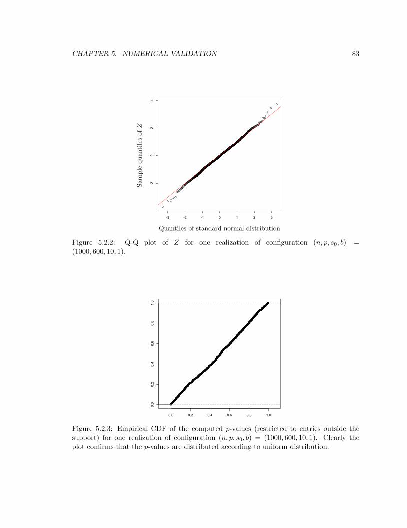
CHAPTER 5. NUMERICAL VALIDATION 83
-3 -2 -1 0 1 2 3
-20
24
Quantiles of standard normal distribution
Sam
ple
qu
anti
les
ofZ
Figure 5.2.2: Q-Q plot of Z for one realization of configuration (n, p, s0, b) =(1000, 600, 10, 1).
0.0 0.2 0.4 0.6 0.8 1.0
0.0
0.2
0.4
0.6
0.8
1.0
Figure 5.2.3: Empirical CDF of the computed p-values (restricted to entries outside thesupport) for one realization of configuration (n, p, s0, b) = (1000, 600, 10, 1). Clearly theplot confirms that the p-values are distributed according to uniform distribution.
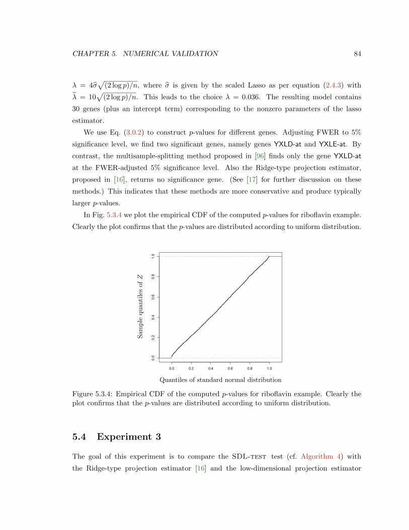
CHAPTER 5. NUMERICAL VALIDATION 84
λ = 4σ√
(2 log p)/n, where σ is given by the scaled Lasso as per equation (2.4.3) with
λ = 10√
(2 log p)/n. This leads to the choice λ = 0.036. The resulting model contains
30 genes (plus an intercept term) corresponding to the nonzero parameters of the lasso
estimator.
We use Eq. (3.0.2) to construct p-values for different genes. Adjusting FWER to 5%
significance level, we find two significant genes, namely genes YXLD-at and YXLE-at. By
contrast, the multisample-splitting method proposed in [96] finds only the gene YXLD-at
at the FWER-adjusted 5% significance level. Also the Ridge-type projection estimator,
proposed in [16], returns no significance gene. (See [17] for further discussion on these
methods.) This indicates that these methods are more conservative and produce typically
larger p-values.
In Fig. 5.3.4 we plot the empirical CDF of the computed p-values for riboflavin example.
Clearly the plot confirms that the p-values are distributed according to uniform distribution.
0.0 0.2 0.4 0.6 0.8 1.0
0.0
0.2
0.4
0.6
0.8
1.0
Quantiles of standard normal distribution
Sam
ple
qu
anti
les
ofZ
Figure 5.3.4: Empirical CDF of the computed p-values for riboflavin example. Clearly theplot confirms that the p-values are distributed according to uniform distribution.
5.4 Experiment 3
The goal of this experiment is to compare the SDL-test test (cf. Algorithm 4) with
the Ridge-type projection estimator [16] and the low-dimensional projection estimator

CHAPTER 5. NUMERICAL VALIDATION 85
0 0.02 0.04 0.06 0.080
0.2
0.4
0.6
0.8
1
1.2
1.4
1.6
Type I error
Aver
age
pow
er
SDL−test (α = 0.05)SDL−test (α = 0.025)Ridge−based regression ( α = 0.05)Ridge−based regression ( α = 0.025)Asymptotic Bound
Figure 5.4.5: Comparison between SDL-test ( Algorithm 4), Ridge-based regression [16]and the asymptotic bound for SDL-test (established in Theorem 4.1.3). Here, p =1000, n = 600, s0 = 25, γ = 0.15.
(LDPE) [149] (cf. Section Subsection 3.4.2) on synthetic data and standard Gaussian de-
sign. we further corroborate the theoretical results of Section 4.1.2 by simulation.
We generate synthetic data from the linear model (1.1.6) with W ∼ N(0, Ip×p) and the
following configurations.
Design matrix: For pairs of values (n, p) = (300, 1000), (600, 1000), (600, 2000), the
design matrix is generated from a realization of n i.i.d. rows Xi ∼ N(0, Ip×p).
Regression parameters: We consider active sets S0 with |S0| = s0 ∈ 10, 20, 25, 50, 100,chosen uniformly at random from the index set 1, · · · , p. We also consider two different
strengths of active parameters θ0,i = γ, for i ∈ S0, with γ ∈ 0.1, 0.15.We examine the performance of SDL-test (cf. Algorithm 4) at significance levels
α = 0.025, 0.05. The experiments are done using glmnet-package in R that fits the entire
Lasso path for linear regression models. Let ε = s0/p and δ = n/p. We do not assume ε is
known, but rather estimate it as ε = 0.25 δ/ log(2/δ). The value of ε is half the maximum
sparsity level ε for the given δ such that the Lasso estimator can correctly recover the
parameter vector if the measurements were noiseless [42, 8]. Provided it makes sense to use
Lasso at all, ε is thus a reasonable ballpark estimate.

CHAPTER 5. NUMERICAL VALIDATION 86
0 0.02 0.04 0.06 0.08 0.10
0.2
0.4
0.6
0.8
1
Asymptotic boundSDL−testRidge−based regressionLDPE
Figure 5.4.6: Comparison between SDL-test , Ridge-based regression [16], andLDPE [149]. The curve corresponds to the asymptotic bound for SDL-test as establishedin Theorem 4.1.3. For the same values of type I error achieved by methods, SDL-testresults in a higher statistical power. Here, p = 1000, n = 600, s0 = 25, γ = 0.15.
The regularization parameter λ is chosen as to satisfy
λd = κ∗τ (5.4.1)
where τ and d are determined in step 2 of the procedure. Here κ∗ = κ∗(ε) is the minimax
threshold value for estimation using soft thresholding in the Gaussian sequence model, see
[44] and Remark B.2.1. Note that τ and d in the equation above depend implicitly upon λ.
Since glmnet returns the entire Lasso path, the value of λ solving the above equation can
be computed by the bisection method.
As mentioned above, the control of type I error is fairly robust for a wide range of values
of λ. However, the above is an educated guess based on the analysis of [42, 8]. We also
tried the values of λ proposed for instance in [133, 16] on the basis of oracle inequalities.
Figure 5.4.5 shows the results of SDL-test and the method of [16] for parameter values
p = 1000, n = 600, s0 = 25, γ = 0.15, and significance levels α ∈ 0.025, 0.05. Each
point in the plot corresponds to one realization of this configuration (there are a total
of 10 realizations). We also depict the theoretical curve (α,G(α, γ0/τ∗)), predicted by
Theorem 4.1.3. The empirical results are in good agreement with the asymptotic prediction.

CHAPTER 5. NUMERICAL VALIDATION 87
We compare SDL-test with the Ridge-based regression method [16] and the low dimen-
sional projection estimator (LDPE ) [149]. Tables 5.4.1 and 5.4.2 summarize the results
for a few configurations (p, n, s0, γ), and α = 0.05, 0.025.
As demonstrated by these results, LDPE [149] and the Ridge-based regression [16] are
both overly conservative. Namely, they achieve smaller type I error than the prescribed
level α and this comes at the cost of a smaller statistical power than our testing procedure.
This is to be expected since the approach of [16] and [149] cover a broader class of design
matrices X, and are not tailored to random designs.
Note that being overly conservative is a drawback, when this comes at the expense
of statistical power. The data analysts should be able to decide the level of statistical
significance α, and obtain optimal statistical power at that level.
The reader might wonder whether the loss in statistical power of methods in [16] and
[149] is entirely due to the fact that these methods achieve a smaller number of false positives
than requested. In Fig. 5.4.6, we run SDL-test , Ridge-based regression [16], and LDPE
for α ∈ 0.01, 0.02, · · · , 0.1 and for 10 realizations of the problem per each value of α. We
plot the average type I error and the average power of each method versus α. As we see even
for the same empirical fraction of type I errors, SDL-test results in a higher statistical
power.

CHAPTER 5. NUMERICAL VALIDATION 88
Method Type I err Type I err Avg. power Avg. power(mean) (std.) (mean) (std)
SDL-test (1000, 600, 50, 0.15) 0.06189 0.01663 0.83600 0.04300Ridge-based regression (1000, 600, 50, 0.15) 0.00989 0.00239 0.35000 0.07071
LDPE (1000, 600, 50, 0.15) 0.03925 0.00588 0.55302 0.07608Asymptotic Bound (1000, 600, 50, 0.15) 0.05 NA 0.84721 NA
SDL-test (1000, 600, 25, 0.15) 0.0572 0.0190 0.8840 0.0638Ridge-based regression (1000, 600, 25, 0.15) 0.0203 0.0052 0.3680 0.1144
LDPE (1000, 600, 25, 0.15) 0.04010 0.00917 0.62313 0.05408Asymptotic Bound (1000, 600, 25, 0.15) 0.05 NA 0.9057 NA
SDL-test (1000, 300, 50, 0.15) 0.05547 0.01554 0.45800 0.06957Ridge-based regression (1000, 300, 50, 0.15) 0.01084 0.00306 0.19200 0.04541
LDPE (1000, 300, 50, 0.15) 0.03022 0.00601 0.23008 0.08180Asymptotic Bound (1000, 300, 50, 0.15) 0.05 NA 0.31224 NA
SDL-test (1000, 300, 25, 0.15) 0.05149 0.01948 0.55600 0.11384Ridge-based regression (1000, 300, 25, 0.15) 0.00964 0.00436 0.32400 0.09324
LDPE (1000, 300, 25, 0.15) 0.04001 0.00531 0.34091 0.06408Asymptotic Bound (1000, 300, 25, 0.15) 0.05 NA 0.51364 NA
SDL-test (2000, 600, 100, 0.1) 0.05037 0.00874 0.44800 0.04940Ridge-based regression (2000, 600, 100, 0.1) 0.01232 0.00265 0.21900 0.03143
LDPE (2000, 600, 100, 0.1) 0.03012 0.00862 0.31003 0.06338Asymptotic Bound (2000, 600, 100, 0.1) 0.05 NA 0.28324 NA
SDL-test (2000, 600, 50, 0.1) 0.05769 0.00725 0.52800 0.08548Ridge-based regression (2000, 600, 50, 0.1) 0.01451 0.00303 0.27000 0.04137
LDPE (2000, 600, 50, 0.1) 0.03221 0.01001 0.35063 0.05848Asymptotic Bound (2000, 600, 50, 0.1) 0.05 NA 0.46818 NA
SDL-test (2000, 600, 20, 0.1) 0.05167 0.00814 0.58000 0.11595Ridge-based regression (2000, 600, 20, 0.1) 0.01879 0.00402 0.34500 0.09846
LDPE (2000, 600, 20, 0.1) 0.04021 0.00608 0.42048 0.08331Asymptotic Bound (2000, 600, 20, 0.1) 0.05 NA 0.58879 NA
SDL-test (2000, 600, 100, 0.15) 0.05368 0.01004 0.64500 0.05104Ridge-based regression (2000, 600, 100, 0.15) 0.00921 0.00197 0.30700 0.04877
LDPE (2000, 600, 100, 0.15) 0.02890 0.00493 0.58003 0.06338Asymptotic Bound (2000, 600, 100, 0.15) 0.05 NA 0.54728 NA
SDL-test (2000, 600, 20, 0.15) 0.04944 0.01142 0.89500 0.07619Ridge-based regression (2000, 600, 20, 0.15) 0.01763 0.00329 0.64000 0.08756
LDPE (2000, 600, 20, 0.15) 0.03554 0.005047 0.73560 0.04008Asymptotic Bound (2000, 600, 20, 0.15) 0.05 NA 0.90608 NA
Table 5.4.1 Comparison between SDL-test, Ridge-based regression [16], LDPE [149] and theasymptotic bound for SDL-test (cf. Theorem 4.1.3) in Experiment 3. The significance level isα = 0.05. The means and the standard deviations are obtained by testing over 10 realizations ofthe corresponding configuration. Here a quadruple such as (1000, 600, 50, 0.1) denotes the values ofp = 1000, n = 600, s0 = 50, γ = 0.1.

CHAPTER 5. NUMERICAL VALIDATION 89
Method Type I err Type I err Avg. power Avg. power(mean) (std.) (mean) (std)
SDL-test (1000, 600, 50, 0.15) 0.02874 0.00546 0.75600 0.07706Ridge-based regression (1000, 600, 50, 0.15) 0.00379 0.00282 0.22800 0.06052
LDPE (1000, 600, 100, 0.1) 0.01459 0.00605 0.41503 0.08482Asymptotic Bound (1000, 600, 50, 0.15) 0.025 NA 0.77107 NA
SDL-test (1000, 600, 25, 0.15) 0.03262 0.00925 0.79200 0.04131Ridge-based regression (1000, 600, 25, 0.15) 0.00759 0.00223 0.28800 0.07729
LDPE (1000, 600, 25, 0.15) 0.01032 0.00490 0.55032 0.07428Asymptotic Bound (1000, 600, 25, 0.15) 0.025 NA 0.84912 NA
SDL-test (1000, 300, 50, 0.15) 0.02916 0.00924 0.36000 0.08380Ridge-based regression (1000, 300, 50, 0.15) 0.00400 0.00257 0.10800 0.05432
LDPE (1000, 300, 50, 0.15) 0.01520 0.00652 0.25332 0.06285Asymptotic Bound (1000, 300, 50, 0.15) 0.025 NA 0.22001 NA
SDL-test (1000, 300, 25, 0.15) 0.03005 0.00894 0.42400 0.08884Ridge-based regression (1000, 300, 25, 0.15) 0.00492 0.00226 0.21600 0.06310
LDPE (1000, 300, 25, 0.15) 0.00881 0.00377 0.31305 0.05218Asymptotic Bound (1000, 300, 25, 0.15) 0.025 NA 0.40207 NA
SDL-test (2000, 600, 100, 0.1) 0.03079 0.00663 0.33000 0.05033Ridge-based regression (2000, 600, 100, 0.1) 0.00484 0.00179 0.11200 0.03615
LDPE (2000, 600, 100, 0.1) 0.01403 0.00970 0.24308 0.06041Asymptotic Bound (2000, 600, 100, 0.1) 0.025 NA 0.19598 NA
SDL-test (2000, 600, 50, 0.1) 0.02585 0.00481 0.41200 0.06197Ridge-based regression (2000, 600, 50, 0.1) 0.00662 0.00098 0.20600 0.03406
LDPE (2000, 600, 50, 0.1) 0.01601 0.00440 0.27031 0.03248Asymptotic Bound (2000, 600, 50, 0.1) 0.025 NA 0.35865 NA
SDL-test (2000, 600, 20, 0.1) 0.02626 0.00510 0.47500 0.10607Ridge-based regression (2000, 600, 20, 0.1) 0.00838 0.00232 0.23500 0.08182
LDPE (2000, 600, 20, 0.1) 0.02012 0.00628 0.34553 0.09848Asymptotic Bound (2000, 600, 20, 0.1) 0.025 NA 0.47698 NA
SDL-test (2000, 600, 100, 0.15) 0.02484 0.00691 0.52700 0.09522Ridge-based regression (2000, 600, 100, 0.15) 0.00311 0.00154 0.22500 0.04007
LDPE (2000, 600, 100, 0.15) 0.01482 0.00717 0.38405 0.03248Asymptotic Bound (2000, 600, 100, 0.15) 0.025 NA 0.43511 NA
SDL-test (2000, 600, 20, 0.15) 0.03116 0.01304 0.81500 0.09443Ridge-based regression (2000, 600, 20, 0.15) 0.00727 0.00131 0.54500 0.09560
LDPE (2000, 600, 20, 0.15) 0.01801 0.00399 0.68101 0.06255Asymptotic Bound (2000, 600, 20, 0.15) 0.025 NA 0.84963 NA
Table 5.4.2 Comparison between SDL-test, Ridge-based regression [16], LDPE [149] and theasymptotic bound for SDL-test (cf. Theorem 4.1.3) in Experiment 3. The significance level isα = 0.025. The means and the standard deviations are obtained by testing over 10 realizations ofthe corresponding configuration. Here a quadruple such as (1000, 600, 50, 0.1) denotes the values ofp = 1000, n = 600, s0 = 50, γ = 0.1

CHAPTER 5. NUMERICAL VALIDATION 90
5.5 Experiment 4
In carrying out comparison between SDL-test , Ridge-type projection estimator [16] and
the low-dimensional projection estimator (LDPE) [149] for correlated Gaussian designs, we
consider the same setup as Experiment 3. The only difference is that the rows of the design
matrix are independently Xi ∼ N(0,Σ). We choose Σ ∈ Rp×p to be a the symmetric matrix
with entries Σjk are defined as follows for j ≤ k
Σjk =
1 if k = j ,
0.1 if k ∈ j + 1, · · · , j + 5
or k ∈ j + p− 5, . . . , j + p− 1,
0 for all other j ≤ k.
(5.5.1)
Elements below the diagonal are given by the symmetry condition Σkj = Σjk. (Notice that
this is a circulant matrix.)
In Fig. 5.5.7(a), we compare SDL-testwith the Ridge-based regression method pro-
posed in [16]. While the type I errors of SDL-test are in good match with the chosen
significance level α, the method of [16] is conservative. As in the case of standard Gaus-
sian designs, this results in significantly smaller type I errors than α and smaller average
power in return. Also, in Fig. 5.5.8, we run SDL-test , Ridge-based regression [16], and
LDPE [149] for α ∈ 0.01, 0.02, · · · , 0.1 and for 10 realizations of the problem per each
value of α. We plot the average type I error and the average power of each method versus
α. As we see, similar to the case of standard Gaussian designs, even for the same empirical
fraction of type I errors, SDL-test results in a higher statistical power.
Tables 5.5.1 and 5.5.2 summarize the results of comparison among these methods for
several configurations (p, n, s0, γ), and α = 0.05, 0.025.
Let z = (zi)pi=1 denote the vector with entries zi ≡ θui /(τ [(Σ−1)ii]
1/2). In Fig. 5.5.7(b)
we plot the normalized histograms of zS0 (in red) and zSc0 (in white), where zS0 and zSc0respectively denote the restrictions of z to the active set S0 and the inactive set Sc0. The
plot clearly exhibits the fact that zSc0 has (asymptotically) standard normal distribution
and the histogram of zS0 appears as a distinguishable bump. This is the core intuition in
defining SDL-test.

CHAPTER 5. NUMERICAL VALIDATION 91
0 0.02 0.04 0.06 0.080
0.1
0.2
0.3
0.4
0.5
0.6
0.7
0.8
0.9
Type I error
Aver
age
pow
er
SDL−test (α = 0.05)SDL−test (α = 0.025)Ridge−based regression ( α = 0.05)Ridge−based regression ( α = 0.025)
(a) Comparison between SDL-test and Ridge-type projectionestimator [16] (cf. Section 3.4.2).
−6 −4 −2 0 2 4 60
0.05
0.1
0.15
0.2
0.25
0.3
0.35
0.4
(b) Normalized histograms of zS0 (in red) and zSc0
(in white) forone realization.
Figure 5.5.7: Numerical results for Experiment 4 and p = 2000, n = 600, s0 = 50, γ = 0.1.

CHAPTER 5. NUMERICAL VALIDATION 92
0 0.05 0.10
0.2
0.4
0.6
0.8
1
SDL−testRidge−based regressionLDPE
Figure 5.5.8: Comparison between SDL-test , Ridge-based regression [16], and LDPE [149]in the setting of Experiment 4. For the same values of type I error achieved by methods,SDL-test results in a higher statistical power. Here, p = 1000, n = 600, s0 = 25, γ = 0.15.
5.6 Experiment 5
In this experiment, we apply SDL-test and the Ridge-type projection estimator [16] on
the UCI communities and crimes dataset [55]. This concerns the prediction of the rate of
violent crime in different communities within US, based on other demographic attributes
of the communities. The dataset consists of a response variable along with 122 predictive
attributes for 1994 communities. Covariates are quantitative, including e.g., the fraction of
urban population or the median family income. We consider a linear model as in (1.1.6)
and hypotheses H0,i. Rejection of H0,i indicates that the i-th attribute is significant in
predicting the response variable.
We perform the following preprocessing steps: (i) Each missing value is replaced by the
mean of the non missing values of that attribute for other communities. (ii) We eliminate
16 attributes to make the ensemble of the attribute vectors linearly independent. Thus we
obtain a design matrix Xtot ∈ Rntot×p with ntot = 1994 and p = 106; (iii) We normalize
each column of the resulting design matrix to have mean zero and `2 norm equal to√ntot.
In order to evaluate various hypothesis testing procedures, we need to know the true
significant variables. To this end, we let θ0 = (XTtotXtot)
−1XTtotY be the least-square es-
timator, using the whole data set. Figure 5.6.9 shows the the entries of θ0. Clearly, only

CHAPTER 5. NUMERICAL VALIDATION 93
Method Type I err Type I err Avg. power Avg. power(mean) (std.) (mean) (std)
SDL-test (1000, 600, 50, 0.15) 0.05179 0.01262 0.81400 0.07604Ridge-based regression (1000, 600, 50, 0.15) 0.01095 0.00352 0.34000 0.05735
LDPE (1000, 600, 50, 0.15) 0.02653 0.00574 0.66800 0.07823Lower bound (1000, 600, 50, 0.15) 0.05 NA 0.84013 0.03810
SDL-test (1000, 600, 25, 0.15) 0.04937 0.01840 0.85600 0.06310Ridge-based regression (1000, 600, 25, 0.15) 0.01969 0.00358 0.46800 0.08011
LDPE (1000, 600, 25, 0.15) 0.01374 0.00709 0.63200 0.07155Lower bound (1000, 600, 25, 0.15) 0.05 NA 0.86362 0.02227
SDL-test (1000, 300, 50, 0.15) 0.05111 0.01947 0.43800 0.09402Ridge-based regression (1000, 300, 50, 0.15) 0.01011 0.00362 0.20200 0.05029
LDPE (1000, 300, 50, 0.15) 0.03621 0.00701 0.37600 0.07127Lower bound (1000, 300, 50, 0.15) 0.05 NA 0.43435 0.03983
SDL-test (1000, 300, 25, 0.15) 0.05262 0.01854 0.53600 0.08044Ridge-based regression (1000, 300, 25, 0.15) 0.01344 0.00258 0.33200 0.08230
LDPE (1000, 300, 25, 0.15) 0.01682 0.00352 0.36800 0.10354Lower bound (1000, 300, 25, 0.15) 0.05 NA 0.50198 0.05738
SDL-test (2000, 600, 100, 0.1) 0.05268 0.01105 0.43900 0.04383Ridge-based regression (2000, 600, 100, 0.1) 0.01205 0.00284 0.21200 0.04392
LDPE (2000, 600, 100, 0.1) 0.028102 0.00720 0.33419 0.04837Lower bound (2000, 600, 100, 0.1) 0.05 NA 0.41398 0.03424
SDL-test (2000, 600, 50, 0.1) 0.05856 0.00531 0.50800 0.05350Ridge-based regression (2000, 600, 50, 0.1) 0.01344 0.00225 0.26000 0.03771
LDPE (2000, 600, 50, 0.1) 0.03029 0.00602 0.37305 0.07281Lower bound (2000, 600, 50, 0.1) 0.05 NA 0.49026 0.02625
SDL-test (2000, 600, 20, 0.1) 0.04955 0.00824 0.57500 0.13385Ridge-based regression (2000, 600, 20, 0.1) 0.01672 0.00282 0.35500 0.08960
LDPE (2000, 600, 20, 0.1) 0.03099 0.00805 0.31350 0.04482Lower bound (2000, 600, 20, 0.1) 0.05 NA 0.58947 0.04472SDL-test (2000, 600, 100, 0.15) 0.05284 0.00949 0.61600 0.06802
Ridge-based regression (2000, 600, 100, 0.15) 0.00895 0.00272 0.31800 0.04131LDPE (2000, 600, 100, 0.15) 0.01022 0.00570 0.35904 0.05205
Lower bound (2000, 600, 100, 0.15) 0.05 NA 0.64924 0.05312SDL-test (2000, 600, 20, 0.15) 0.05318 0.00871 0.85500 0.11891
Ridge-based regression (2000, 600, 20, 0.15) 0.01838 0.00305 0.68000 0.12517LDPE (2000, 600, 20, 0.15) 0.02512 0.00817 0.36434 0.05824
Lower bound (2000, 600, 20, 0.15) 0.05 NA 0.87988 0.03708
Table 5.5.1 Comparison between SDL-test, Ridge-based regression [16], LDPE [149] and the lowerbound for the statistical power of SDL-test (cf. Theorem 4.2.4) in Experiment 4. The significancelevel is α = 0.05. The means and the standard deviations are obtained by testing over 10 realizationsof the corresponding configuration. Here a quadruple such as (1000, 600, 50, 0.1) denotes the valuesof p = 1000, n = 600, s0 = 50, γ = 0.1

CHAPTER 5. NUMERICAL VALIDATION 94
Method Type I err Type I err Avg. power Avg. power(mean) (std.) (mean) (std)
SDL-test (1000, 600, 50, 0.15) 0.02579 0.00967 0.71800 0.03824Ridge-based regression (1000, 600, 50, 0.15) 0.00326 0.00274 0.21000 0.05437
LDPE (1000, 600, 50, 0.15) 0.01245 0.00391 0.64807 0.065020Lower bound (1000, 600, 50, 0.15) 0.025 NA 0.75676 0.05937
SDL-test (1000, 600, 25, 0.15) 0.02462 0.00866 0.75600 0.12429Ridge-based regression (1000, 600, 25, 0.15) 0.01077 0.00346 0.30400 0.08262
LDPE (1000, 600, 25, 0.15) 0.00931 0.00183 0.68503 0.17889Lower bound (1000, 600, 25, 0.15) 0.025 NA 0.80044 0.05435
SDL-test (1000, 300, 50, 0.15) 0.02646 0.01473 0.39200 0.11478Ridge-based regression (1000, 300, 50, 0.15) 0.00368 0.00239 0.15000 0.04137
LDPE (1000, 300, 50, 0.15) 0.01200 0.00425 0.28800 0.09654Lower bound (1000, 300, 50, 0.15) 0.025 NA 0.36084 0.04315
SDL-test (1000, 300, 25, 0.15) 0.02400 0.00892 0.42400 0.09834Ridge-based regression (1000, 300, 25, 0.15) 0.00513 0.00118 0.18800 0.07786
LDPE (1000, 300, 25, 0.15) 0.00492 0.00169 0.24500 0.07483Lower bound (1000, 300, 25, 0.15) 0.025 NA 0.42709 0.03217
SDL-test (2000, 600, 100, 0.1) 0.03268 0.00607 0.32600 0.07412Ridge-based regression (2000, 600, 100, 0.1) 0.00432 0.00179 0.14100 0.05065
LDPE (2000, 600, 100, 0.1) 0.01240 0.00572 0.20503 0.09280Lower bound (2000, 600, 100, 0.1) 0.025 NA 0.32958 0.03179
SDL-test (2000, 600, 50, 0.1) 0.03108 0.00745 0.41800 0.04662Ridge-based regression (2000, 600, 50, 0.1) 0.00687 0.00170 0.18800 0.06680
LDPE (2000, 600, 50, 0.1) 0.014005 0.00740 0.25331 0.04247Lower bound (2000, 600, 50, 0.1) 0.025 NA 0.40404 0.06553
SDL-test (2000, 600, 20, 0.1) 0.02965 0.00844 0.38500 0.07091Ridge-based regression (2000, 600, 20, 0.1) 0.00864 0.00219 0.22500 0.07906
LDPE (2000, 600, 20, 0.1) 0.01912 0.00837 0.31551 0.06288Lower bound (2000, 600, 20, 0.1) 0.025 NA 0.47549 0.06233SDL-test (2000, 600, 100, 0.15) 0.026737 0.009541 0.528000 0.062681
Ridge-based regression (2000, 600, 100, 0.15) 0.002947 0.000867 0.236000 0.035653LDPE (2000, 600, 100, 0.15) 0.01012 0.00417 0.36503 0.05823
Lower bound (2000, 600, 100, 0.15) 0.025 NA 0.54512 0.05511SDL-test (2000, 600, 20, 0.15) 0.03298 0.00771 0.79000 0.12202
Ridge-based regression (2000, 600, 20, 0.15) 0.00732 0.00195 0.53500 0.07091LDPE (2000, 600, 20, 0.15) 0.01302 0.00711 0.60033 0.03441
Lower bound (2000, 600, 20, 0.15) 0.025 NA 0.81899 0.03012
Table 5.5.2 Comparison between SDL-test, Ridge-based regression [16], LDPE [149] and thelower bound for the statistical power of SDL-test (cf. Theorem 4.2.4) in Experiment 4. Thesignificance level is α = 0.025. The means and the standard deviations are obtained by testingover 10 realizations of the corresponding configuration. Here a quadruple such as (1000, 600, 50, 0.1)denotes the values of p = 1000, n = 600, s0 = 50, γ = 0.1

CHAPTER 5. NUMERICAL VALIDATION 95
0 20 40 60 80 100
-0.10
-0.05
0.00
0.05
0.10
0.15
0.20
θ 0
θ0
Figure 5.6.9: Parameter vector θ0 for the communities data set.
a few entries have non negligible values which correspond to the predictive attributes. In
computing type I errors and powers, we take the elements in θ0 with magnitude larger than
0.04 as active and the others as inactive.
In order to validate our approach in the high-dimensional p > n regime, we take random
subsamples of the communities (hence subsamples of the rows of Xtot) of size n = 84. We
compare SDL-test with the method of [16], over 20 realizations and significance levels
α = 0.01, 0.025, 0.05. The fraction of type I errors and statistical power is computed by
comparing to θ0. Table 5.6.1 summarizes the results. As the reader can see, Ridge-type
projection estimator is very conservative yielding to no type-I errors but a much smaller
power than SDL-test.
In Table 5.6.2, we report the relevant features obtained from the whole dataset as
described above, corresponding to the nonzero entries in θ0. We also report the features
identified as relevant by SDL-test and those identified as relevant by Ridge-type projection
estimator, from one random subsample of communities of size n = 84. Features description
is available in [55].
Finally, in Fig. 5.6.10 we plot the normalized histograms of vS0 (in red) and vSc0 (in
white). Recall that v = (vi)pi=1 denotes the vector with vi ≡ θui /(τ [(Σ−1)ii]
1/2). Further,
vS0 and vSc0 respectively denote the restrictions of v to the active set S0 and the inactive set
Sc0. This plot demonstrates that vSc0 has roughly standard normal distribution as expected

CHAPTER 5. NUMERICAL VALIDATION 96
−10 0 10 20 300
0.1
0.2
0.3
0.4
0.5
Figure 5.6.10: Normalized histogram of vS0 (in red) and vSc0 (in white) for the communitiesdata set.
by the developed theory in Chapter 4.
Method Type I err Avg. power(mean) (mean)
SDL-test (α = 0.05) 0.0172043 0.4807692Ridge-based regression 0 0.1423077
SDL-test (α = 0.025) 0.01129032 0.4230769Ridge-based regression 0 0.1269231
SDL-test (α = 0.01) 0.008602151 0.3576923Ridge-based regression 0 0.1076923
Table 5.6.1 Simulation results for the communities data set.

CHAPTER 5. NUMERICAL VALIDATION 97
Relevant features
racePctHisp, PctTeen2Par, PctImmigRecent, PctImmigRec8, Pc-tImmigRec10, PctNotSpeakEnglWell, OwnOccHiQuart, Num-Street, PctSameState85, LemasSwFTFieldPerPop, LemasTotRe-qPerPop, RacialMatchCommPol, PolicOperBudg
α = 0.01Relevant features
(SDL-test )
racePctHisp, PctTeen2Par, PctImmigRecent, PctImmigRec8, Pc-tImmigRec10, PctNotSpeakEnglWell, OwnOccHiQuart, Num-Street, PctSameState85, LemasSwFTFieldPerPop, LemasTotRe-qPerPop, RacialMatchCommPol, PolicOperBudg
Relevant features(Ridge-based regression)
racePctHisp, PctSameState85
α = 0.025Relevant features
(SDL-test )
racePctHisp, PctTeen2Par, PctImmigRecent, PctImmigRec8, Pc-tImmigRec10, PctNotSpeakEnglWell, PctHousOccup, OwnOc-cHiQuart, NumStreet, PctSameState85, LemasSwFTFieldPer-Pop, LemasTotReqPerPop, RacialMatchCommPol, PolicOper-Budg
Relevant features(Ridge-based regression)
racePctHisp, PctSameState85
α = 0.05Relevant features
(SDL-test )
racePctHisp, PctUnemployed, PctTeen2Par, PctImmigRecent,PctImmigRec8, PctImmigRec10, PctNotSpeakEnglWell, Pc-tHousOccup, OwnOccHiQuart, NumStreet, PctSameState85,LemasSwornFT, LemasSwFTFieldPerPop, LemasTotReqPerPop,RacialMatchCommPol, PctPolicWhite
Relevant features(Ridge-based regression)
racePctHisp, PctSameState85
Table 5.6.2 The relevant features (using the whole dataset) and the relevant features pre-dicted by SDL-test and the Ridge-type projection estimator [16] for a random subsampleof size n = 84 from the communities. The false positive predictions are in red.

Chapter 6
Proof of Theorems in Part I
This chapter contains proofs of Theorems and technical lemmas stated in Chapter 2.
6.1 Proof of Theorems in Chapter 2
6.1.1 Proof of Theorem 2.3.3
Substituting Y = Xθ0 +W in the definition (2.3.2), we get
θ∗ = θn +1
nMXTX(θ0 − θn) +
1
nMXTW
= θ0 +1√nZ +
1√n
∆ ,(6.1.1)
with Z,∆ defined as per the theorem statement. Further Z is Gaussian with the stated
covariance because it is a linear function of the Gaussian vector W ∼ N(0, σ2 Ip×p).
We are left with the task of proving the bound (2.3.6) on ∆. Note that by definition
(2.3.1), we have
‖∆‖∞ ≤√n |M Σ− I|∞ ‖θn − θ0‖1 =
√nµ∗‖θn − θ0‖1 . (6.1.2)
By [19, Theorem 6.1, Lemma 6.2], we have, for any λ ≥ 4σ√
2K log(pet2/2)/n
P(‖θn − θ0‖1 ≥
4λs0
φ20
)≤ 2 e−t
2/2 . (6.1.3)
(More precisely, we consider the trivial generalization of [19, Lemma 6.2] to the case
98

CHAPTER 6. PROOF OF THEOREMS IN PART I 99
(XTX/n)ii ≤ K, instead of (XTX/n)ii = 1 for all i ∈ [p].)
Substituting Eq. (6.1.2) in the last bound, we get
P(‖∆‖∞ ≥
4λµ∗s0√n
φ20
)≤ 2 e−t
2/2 . (6.1.4)
Finally, the claim follows by selecting t so that et2/2 = pc0 .
6.1.2 Proof of Theorem 2.3.4.(a)
Note that the event En requires two conditions. Hence, its complement is given by
En(φ0, s0,K)c = B1,n(φ0, s0) ∪ B2,n(K) , (6.1.5)
B1,n(φ0, s0) ≡
X ∈ Rn×p : minS: |S|≤s0
φ(Σ, S) < φ0, Σ = (XTX/n), (6.1.6)
B2,n(K) ≡
X ∈ Rn×p : maxi∈[p]
Σi,i > K, Σ = (XTX/n). (6.1.7)
We will bound separately the probability of B1,n and the probability of B2,n. The claim of
Theorem 2.3.4.(a) follows by union bound.
6.1.2.1 Controlling B1,n(φ0, s0)
It is also useful to recall the notion of restricted eigenvalue, introduced by Bickel, Ritov and
Tsybakov [14].
Definition 6.1.1. Given a symmetric matrix Q ∈ Rp×p an integer s0 ≥ 1, and L > 0, the
restricted eigenvalue of Q is defined as
φ2RE(Q, s0, L) ≡ min
S⊆[p],|S|≤s0minθ∈Rp
〈θ,Q θ〉‖θS‖22
: θ ∈ Rp, ‖θSc‖1 ≤ L‖θS‖1. (6.1.8)
[116] proves that, if the population covariance satisfies the restricted eigenvalue condi-
tion, then the sample covariance satisfies it as well, with high probability. More precisely,
by [116, Theorem 6] we have
P(φRE(Σ, s0, 3) ≥ 1
2φRE(Σ, s0, 9)
)≥ 1− 2e−n/(4c∗κ
4) , (6.1.9)
for some c∗ ≤ 2000, m ≡ 6×10⁴s0C2max/φ
2RE(Σ, s0, 9), and every n ≥ 4c∗mκ
4 log(120ep/m).

CHAPTER 6. PROOF OF THEOREMS IN PART I 100
Note that φRE(Σ, s0, 9) ≥ σmin(Σ)1/2 ≥√Cmin, and by Cauchy-Schwartz,
minS:|S|≤s0
φ(Σ, S) ≥ φRE(Σ, s0, 3) .
With the definitions in the statement (cf. Eq. (2.3.8)), we therefore have
P(
minS:|S|≤s0
φ(Σ, S) ≥ 1
2
√Cmin
)≥ 1− 2e−c1n . (6.1.10)
Equivalently, P(B1,n(φ0, s0)) ≤ 2 e−c1n.
6.1.2.2 Controlling B2,n(K)
By definition
Σii − 1 =1
n
n∑`=1
(〈X`, ei〉2 − 1) =1
n
n∑`=1
u`, . (6.1.11)
Note that u` are independent centered random variables. Further, (recalling that, for any
random variables U, V , ‖U + V ‖ψ1 ≤ ‖U‖ψ1 + ‖V ‖ψ1 , and ‖U2‖ψ1 ≤ 2‖U‖2ψ2) they are
subexponential with subexponential norm
‖u`‖ψ1 ≤ 2‖〈X`, ei〉2‖ψ1 ≤ 4‖〈X`, ei〉‖2ψ1
≤ 4‖〈Σ−1/2X`,Σ1/2ei〉‖2ψ1
≤ 4κ2‖Σ1/2ei‖22 = 4κ2Σii = 4κ2 .
By Bernstein-type inequality for centered subexponential random variables, cf. [136], we
get
P 1
n
∣∣∣ n∑`=1
u`
∣∣∣ ≥ ε ≤ 2 exp[− n
6min
((ε
4eκ2)2,
ε
4eκ2
)]. (6.1.12)
Hence, for all ε such that ε/(eκ2) ∈ [√
(48 log p)/n, 4],
P(
maxi∈[p]
Σii ≥ 1 + ε)≤ 2p exp
(− nε2
24e2κ4
)≤ 2e−c1n , (6.1.13)
which implies P(X ∈ B2,n(K)) ≤ 2 e−c1n for allK−1 ≥ 20κ2√
(log p)/n ≥√
(48e2κ4 log p)/n.

CHAPTER 6. PROOF OF THEOREMS IN PART I 101
6.1.3 Proof of Theorem 2.3.4.(b)
Obviously, we have
µmin(X) ≤∣∣Σ−1Σ− I
∣∣ , (6.1.14)
and hence the statement follows immediately from the following estimate.
Lemma 6.1.2. Consider a random design matrix X ∈ Rp×p, with i.i.d. rows having mean
zero and population covariance Σ. Assume that
(i) We have σmin(Σ) ≥ Cmin > 0, and σmax(Σ) ≤ Cmax <∞.
(ii) The rows of XΣ−1/2 are sub-gaussian with κ = ‖Σ−1/2X1‖ψ2.
Let Σ = (XTX)/n be the empirical covariance. Then, for any constant C > 0, the following
holds true.
P∣∣∣Σ−1Σ− I
∣∣∣∞≥ a
√log p
n
≤ 2p−c2 , (6.1.15)
with c2 = (a2Cmin)/(24e2κ4Cmax)− 2.
Proof of Lemma 6.1.2. The proof is based on Bernstein-type inequality for sub-exponential
random variables [136]. Let X` = Σ−1/2X`, for ` ∈ [n], and write
Z ≡ Σ−1Σ− I =1
n
n∑`=1
Σ−1X`X
T` − I
=
1
n
n∑`=1
Σ−1/2X`X
T` Σ1/2 − I
.
Fix i, j ∈ [p], and for ` ∈ [n], let v(ij)` = 〈Σ−1/2
i,· , X`〉〈Σ1/2j,· , X`〉−δi,j , where δi,j = 1i=j. No-
tice that E(v(ij)` ) = 0, and the v
(ij)` are independent for ` ∈ [n]. Also, Zi,j = (1/n)
∑n`=1 v
(ij)` .
By [136, Remark 5.18], we have
‖v(ij)` ‖ψ1 ≤ 2‖〈Σ−1/2
i,· , X`〉〈Σ1/2j,· , X`〉‖ψ1 .

CHAPTER 6. PROOF OF THEOREMS IN PART I 102
Moreover, for any two random variables X and Y , we have
‖XY ‖ψ1 = supp≥1
p−1E(|XY |p)1/p
≤ supp≥1
p−1E(|X|2p)1/2p E(|Y |2p)1/2p
≤ 2(
supq≥2
q−1/2E(|X|q)1/q)(
supq≥2
q−1/2E(|Y |q)1/q)
≤ 2‖X‖ψ2 ‖Y ‖ψ2 .
Hence, by assumption (ii), we obtain
‖v(ij)` ‖ψ1 ≤ 2‖〈Σ−1/2
i,· , X`〉‖ψ2‖〈Σ1/2j,· , X`〉‖ψ2
≤ 2‖Σ−1/2i,· ‖2‖Σ
1/2j,· ‖2κ
2 ≤ 2√Cmax/Cmin κ
2 .
Let κ′ = 2√Cmax/Cminκ
2. Applying Bernstein-type inequality for centered sub-exponential
random variables [136], we get
P 1
n
∣∣∣ n∑`=1
v(ij)`
∣∣∣ ≥ ε ≤ 2 exp[− n
6min
((ε
eκ′)2,
ε
eκ′
)].
Choosing ε = a√
(log p)/n, and assuming n ≥ [a/(eκ′)]2 log p, we arrive at
P
1
n
∣∣∣ n∑`=1
v(ij)`
∣∣∣ ≥ a√ log p
n
≤ 2p−a
2/(6e2κ′2) .
The result follows by union bounding over all possible pairs i, j ∈ [p].
6.1.4 Proof of Theorem 2.2.1
The KKT condition for the Lasso estimator reads
1
nXT(Y −Xθn) = λv(θn) ,

CHAPTER 6. PROOF OF THEOREMS IN PART I 103
with v(θn) ∈ Rp being a vector in the subgradient of the `1 norm at θn. Adding θn − θ0 to
both sides, and taking expectation over the noise, we get
Bias(θ∗) = Bias(θn) + λEv(θn)|X , (6.1.16)
where θ∗ is a debiased estimator of the general form (2.3.2), for M = I.
In the following, we show that there exist a set of design matrices Bn ⊆ Rn×p satisfying
the probability bound (2.2.3) and a constant 0 < c∗∗ ≤ 4800, such that for X ∈ Bn we have
‖Bias(θ∗)‖∞ ≤ c∗∗σs0 log p
n, (6.1.17)
‖Ev(θn)|X‖∞ ≥ 2
3. (6.1.18)
Note that by applying triangle inequality to (6.1.16), we have
‖Bias(θn)‖∞ ≥ λ‖Ev(θn)|X‖∞ − ‖Bias(θ∗)‖∞ .
Using the bounds (6.1.17) and (6.1.18) in the above inequality, and invoking the assumption
n ≥ (3c∗∗σs0/c)2 log p, we obtain the desired result.
We begin with proving inequality (6.1.17). By Theorem 2.3.4.(a), we have
P(X ∈ En(1/2, s0, 3/2)
)≥ 1− 4 e−c1n . (6.1.19)
Further, by Lemma 6.1.2, with Σ ≡ XTX/n, we have
P(µ∗(X; I) ≤ 30
√log p
n
)≥ 1− 2 p−3 . (6.1.20)
Hence, defining
Bn ≡ En(1/2, s0, 3/2) ∩
X ∈ Rn×p : µ∗(X; I) ≤ 30
√log p
n
(6.1.21)
we have the desired probability bound (2.2.3). Let θn = θn(Y,X; I, λ). By Theorem 2.3.3,
we have, for any X ∈ Bn
θ∗ = θ0 +1√nZ +
1√n
∆ , Z|X ∼ N(0, σ2Σ) , (6.1.22)

CHAPTER 6. PROOF OF THEOREMS IN PART I 104
and further
P‖∆‖∞ ≥
480cσs0 log p√n
∣∣∣X ≤ 2p1−(c2/48) . (6.1.23)
Let L = (480σs0 log p)/√n. Then,
‖Bias(θu)‖∞ ≤1√nE‖∆‖∞
∣∣X=
L√n
∫ ∞0
P‖∆‖∞ ≥ Lc
∣∣∣X dc
≤ 2L√n
∫ ∞0
min(1, p1−(c2/48)) dc ≤ 10L√n,
where (6.1.23) is used in the second inequality. Therefore, for some constant c∗∗ ≤ 4800,
we have
‖Bias(θ∗)‖∞ ≤ c∗∗σs0 log p
n. (6.1.24)
We next prove inequality (6.1.18). Note that v(θn)i = 1 whenever θni > 0, and |v(θn)i| ≤1 for all coordinates i. Therefore, letting b0 ≡ 480cσ(s0 log p)/n we have
1− Ev(θn)i|X ≤ 2P(θni ≤ 0
∣∣∣X) ≤ 2P(θui ≤ λ
∣∣∣X) (6.1.25)
≤ 2P(θ0,i +
1√nZi +
1√n
∆i ≤ λ∣∣∣X)
≤ 2P( 1√
nZi ≤ λ+ b0 − θ0,i
∣∣∣X)+ 2P(‖∆‖∞ >
√nb0
)= 2Φ
((λ+ b0 − θ0,i)
√n/(σ2Σii)
)+ 4p1−(c2/48)
≤ 2Φ(
(λ+ b0 − θ0,i)√
2n/(3σ2))
+ 4p1−(c2/48) (6.1.26)
with Φ(x) the standard normal distribution function. Here, we used the relation θu =
θ+λv(θ) in Eq. (6.1.25). Further, Eq. (6.1.26) holds because maxi∈[p] Σii ≤ 3/2 on Bn. We
then choose θ0 so that θ0,i ≥ b0 + λ+√
30σ2/n, for i ∈ supp(θ0). We therefore obtain
Ev(θn)i|X ≥ 1− 2Φ(−√
20)− 4p1−(c2/48) ≥ 2
3, (6.1.27)
where in the last step we used the assumption p ≥ 1348/(c2−48).

CHAPTER 6. PROOF OF THEOREMS IN PART I 105
This completes the proof of the theorem.
6.1.5 Proof of Theorem 2.3.5
Let
∆0 ≡(16ac σ
Cmin
)s0 log p√n
(6.1.28)
be a shorthand for the bound on ‖∆‖∞ appearing in Eq. (2.3.14). Then we have
P(‖∆‖∞ ≥ ∆0
)≤P(‖∆‖∞ ≥ ∆0
∩ En(
√Cmin/2, s0, 3/2) ∩ Gn(a)
)+ P
(En(√Cmin/2, s0, 3/2)
)+ P
(Gcn(a)
)≤P(‖∆‖∞ ≥ ∆0
∩ En(
√Cmin/2, s0, 3/2) ∩ Gn(a)
)+ 4 e−c1n + 2 p−c2 ,
where, in the firsr equation Ac denotes the complement of event A and the second inequality
follows from Theorem 2.3.4. Notice, in particular, that the bound (2.3.8) can be applied
for K = 3/2 since, under the present assumptions 20κ2√
(log p)/n ≤ 1/2. Finally
P(‖∆‖∞ ≥ ∆0
∩ En(
√Cmin/2, s0, 3/2) ∩ Gn(a)
)≤ sup
X∈En(√Cmin/2,s0,3/2)∩Gn(a)
P(‖∆‖∞ ≥ ∆0
∣∣∣X) ≤ 2 p−c0 . (6.1.29)
Here the last inequality follows from Theorem 2.3.3 applied per given X ∈ En(√Cmin/2, s0, 3/2)∩
Gn(a) and hence using the bound (2.3.6) with φ0 =√Cmin/2, K = 3/2, µ∗ = a
√(log p)/n.
6.1.6 Proof of Corollary 2.3.7
By Theorem 2.3.3, for any X ∈ En(√Cmin/2, s0, 3/2) ∩ Gn(a), we have
P‖∆‖∞ ≥ Lc
∣∣∣X ≤ 2 p1−(c2/48) , L ≡ 16aσ
Cmin
s0 log p√n
. (6.1.30)

CHAPTER 6. PROOF OF THEOREMS IN PART I 106
This is obtained by setting φ0 =√Cmin/2, K = 3/2, µ∗ = a
√(log p)/n in Eq. (2.3.6).
Hence
‖Bias(θu)‖∞ ≤1√nE‖∆‖∞
∣∣X=
L√n
∫ ∞0
P‖∆‖∞ ≥ Lc
∣∣∣X dc
≤ 2L√n
∫ ∞0
min(1, p1−(c2/48)) dc ≤ 10L√n, (6.1.31)
which coincides with Eq. (2.3.17). The probability estimate (2.3.18) simply follows from
Theorem 2.3.4 using union bound.
6.1.7 Proof of Lemma 2.4.2
We will prove that, under the stated assumptions
lim supn→∞
sup‖θ0‖0≤s0
P
√n(θui − θ0,i)
σ[M ΣMT]1/2i,i
≤ x
≤ Φ(x) . (6.1.32)
A matching lower bound follows by a completely analogous argument.
Notice that by Eq. (2.3.13), we have
√n(θui − θ0,i)
σ[M ΣMT]1/2ii
=eTi MXTW
σ[M ΣMT]1/2ii
+∆i
σ[M ΣMT]1/2ii
. (6.1.33)
Let V = XMTei/(σ[M ΣMT]1/2ii ) and Z ≡ V TW . We claim that Z ∼ N(0, 1). To see this,
note that ‖V ‖2 = 1, and V and W are independent. Hence,
P(Z ≤ x) = EP(V TW ≤ x|V ) = EΦ(x)|V = Φ(x) , (6.1.34)

CHAPTER 6. PROOF OF THEOREMS IN PART I 107
which proves our claim. In order to prove Eq. (6.1.32), fix ε > 0 and write
P
(√n(θui − θ0,i)
σ[M ΣMT]1/2i,i
≤ x
)= P
(σ
σZ +
∆i
σ[M ΣMT]1/2i,i
≤ x
)
≤ P(σσZ ≤ x+ ε
)+ P
(|∆i|
σ[M ΣMT]1/2i,i
≥ ε
)
≤ P(Z ≤ x+ 2ε+ ε|x|
)+ P
(|∆i|
σ[M ΣMT]1/2i,i
≥ ε
)
+ P(∣∣∣ σσ− 1∣∣∣ ≥ ε) .
By taking the limit and using the assumption (2.4.1), we obtain
lim supn→∞
sup‖θ0‖0≤s0
P
(√n(θui − θ0,i)
σ[M ΣMT]1/2i,i
≤ x
)≤
Φ(x+ 2ε+ ε|x|) + lim supn→∞
sup‖θ0‖0≤s0
P
(|∆i|
σ[M ΣMT]1/2i,i
≥ ε
).
Since ε > 0 is arbitrary, it is therefore sufficient to show that the limit on the right hand
side vanishes for any ε > 0.
Note that [M ΣMT]i,i ≥ 1/(4Σii) for all n large enough, by Lemma 2.4.1, and since
µ = a√
(log p)/n→ 0 as n, p→∞. We have therefore
P
(|∆i|
σ[M ΣMT]1/2i,i
≥ ε
)≤ P
( 2
σΣ
1/2ii |∆i| ≥ ε
)≤ P
( 5
σ|∆i| ≥ ε
)+ P
( σσ≤ 1
2
)+ P(Σii ≥
√2) .
Note that P((σ/σ) ≤ 1/2
)→ 0 by assumption (2.4.1), and P(Σii ≥
√2) → 0 by Theorem
2.3.4.(b). Hence
lim supn→∞
sup‖θ0‖0≤s0
P
(|∆i|
σ[M ΣMT]1/2i,i
≥ ε
)≤ lim sup
n→∞sup
‖θ0‖0≤s0P(‖∆‖∞ ≥
εσ
5
)≤ lim sup
n→∞
(4 e−c1n + 4 p−(c0∧c2)
)= 0 ,

CHAPTER 6. PROOF OF THEOREMS IN PART I 108
where the last inequality follows from Eq. (2.3.14), recalling that s0 = o(√n/ log p) and
hence (16acs0 log p)/(Cmin√n) ≤ ε/5 for all n large enough.
This completes the proof of Eq. (6.1.32). The matching lower bound follows by the same
argument.
6.1.8 Proof of Theorem 2.4.6
Under the assumptions of Theorem 2.3.5 and assuming s0 = o(√n/ log p), we have
√n(θu − θ0) =
1√nMXTW + ∆
with ‖∆‖∞ = o(1). Using Lemma 2.4.1, we have
√n(θui − θ0,i)
σ[M ΣMT]1/2i,i
= Zi + o(1) , with Zi ≡1√n
mTi XTW
σ[mTi Σmi]1/2
.
The following lemma characterizes the limiting distribution of Zi|X which implies the
validity of the proposed confidence intervals.
Lemma 6.1.3. Suppose that the noise variables Wi are independent with E(Wi) = 0, and
E(W 2i ) = σ2, and E(|Wi|2+a) ≤ C σ2+a for some a > 0. Let M = (m1, . . . ,mp)
T be the
matrix with rows mTi obtained by solving optimization problem (2.4.12). For i ∈ [p], define
Zi =1√n
mTi XTW
σ[mTi Σmi]1/2
.
Under the assumptions of Theorem 2.3.5, for any sequence i = i(n) ∈ [p], and any x ∈ R,
we have
limn→∞
P(Zi ≤ x|X) = Φ(x) .
Lemma 6.1.3 is proved in Appendix A.3.

CHAPTER 6. PROOF OF THEOREMS IN PART I 109
6.2 Proof of Theorems in Chapter 3
6.2.1 Proof of Theorem 3.1.1
We begin with proving Eq. (3.1.3). Defining Zi ≡√n(θui − θ0,i)/(σ[M ΣMT]
1/2i,i ), we have
limn→∞
αn(Ti) = limn→∞
supθ0
P(Pi ≤ α) : i ∈ [p], ‖θ0‖0 ≤ s0, θ0,i = 0
= lim
n→∞supθ0
P(
Φ−1(1− α
2) ≤
√n|θui |
σ[M ΣMT]1/2i,i
): i ∈ [p], ‖θ0‖0 ≤ s0, θ0,i = 0
= lim
n→∞supθ0
P(
Φ−1(1− α
2) ≤ |Zi|
): i ∈ [p], ‖θ0‖0 ≤ s0
≤ α ,
where the last inequality follows from Lemma 2.4.2.
We next prove Eq. (3.1.4). Recall that Σ−1·,i is a feasible solution of (2.3.11), for 1 ≤ i ≤ p
with probability at least 1− 2p−c2 , as per Lemma 6.1.2). On this event, letting mi be the
solution of the optimization problem (2.3.11), we have
mTi Σmi ≤ Σ−1
i,· ΣΣ−1·,i
= (Σ−1i,· ΣΣ−1
·,i − Σ−1ii ) + Σ−1
i,i
=1
n
N∑j=1
(V 2j − Σ−1
ii ) + Σ−1i,i ,
where Vj = Σ−1i,· Xj are i.i.d. random variables with E(V 2
j ) = Σ−1ii and sub-gaussian norm
‖Vj‖ψ2 ≤ ‖Σ−1/2i,· ‖2‖Σ
−1/2Xj‖ψ2 ≤ κ√
Σ−1i,i .
Letting Uj = V 2j −Σ−1
ii , we have that Uj is zero mean and sub-exponential with ‖Uj‖ψ1 ≤2‖V 2
j ‖ψ1 ≤ 4‖Vj‖2ψ2≤ 4κ2Σ−1
ii ≤ 4κ2σmin(Σ)−1 ≤ 4κ2C−1min ≡ κ′. Hence, by applying
Bernstein inequality (as, for instance, in the proof of Lemma 6.1.2), we have, for ε ≤ eκ′,
P(mTi Σmi ≥ Σ−1
i,i + ε)≤ 2 e−(n/6)(ε/eκ′)2
+ 2 p−c2 .
We can make c2 ≥ 2 by a suitable choice of a and therefore, by Borel-Cantelli we have the

CHAPTER 6. PROOF OF THEOREMS IN PART I 110
following almost surely
lim supn→∞
[mTi Σmi − Σ−1
i,i ] ≤ 0 . (6.2.1)
Now we are ready to prove the lower bound for the power. Let z∗ ≡ Φ−1(1 − α/2).
Then,
lim infn→∞
1− βn(Ti; γ)
1− β∗i,n(γ)
= lim infn→∞
1
1− β∗i,n(γ)infθ0
P(Pi ≤ α) : ‖θ0‖0 ≤ s0, |θ0,i| ≥ γ
= lim inf
n→∞
1
1− β∗i,n(γ)infθ0
P(z∗ ≤
√n|θui |
σ[M ΣMT]1/2i,i
): ‖θ0‖0 ≤ s0, |θ0,i| ≥ γ
= lim inf
n→∞
1
1− β∗i,n(γ)infθ0
P(z∗ ≤
∣∣∣Zi +
√nθ0,i
σ[M ΣMT]1/2i,i
∣∣∣) : ‖θ0‖0 ≤ s0, |θ0,i| ≥ γ
(a)
≥ lim infn→∞
1
1− β∗i,n(γ)infθ0
P(z∗ ≤
∣∣∣Zi +
√nγ
σ[Σ−1i,i ]1/2
∣∣∣) : ‖θ0‖0 ≤ s0
= lim inf
n→∞
1
1− β∗i,n(γ)
1− Φ
(z∗ −
√nγ
σ[Σ−1i,i ]1/2
)+ Φ
(− z∗ −
√nγ
σ[Σ−1i,i ]1/2
)= lim inf
n→∞
1
1− β∗i,n(γ)G(α,
√nγ
σ[Σ−1i,i ]1/2
)= 1 .
Here (a) follows from Eq. (6.2.1) and the fact |θ0,i| ≥ γ.
6.2.2 Proof of Theorem 3.2.1
Let Fp,s0 ≡ x ∈ Rp : ‖x‖0 ≤ s0, and fix ε ∈ (0, 1/10). By definition,
FWER(TF, n) = supθ0∈Fp,s0
P
∃i ∈ [p] \ supp(θ0), s.t.
√n |θui − θ0,i|
σ[M ΣMT]1/2i,i
≥ Φ−1(
1− α
2p
)
≤ supθ0∈Fp,s0
P
∃i ∈ [p] \ supp(θ0), s.t.
√n |θui − θ0,i|
σ[M ΣMT]1/2i,i
≥ (1− ε)Φ−1(
1− α
2p
)
+ supθ0∈Fp,s0
P(∣∣∣ σσ− 1∣∣∣ ≥ ε) .

CHAPTER 6. PROOF OF THEOREMS IN PART I 111
Since the second term vanishes as n → ∞ by Eq. (2.4.1). Using Bonferroni inequality,
letting zα(ε) ≡ (1− ε)Φ−1(1− α
2p
), we have
lim supn→∞
FWER(TF, n) ≤ lim supn→∞
p∑i=1
supθ0∈Fp,s0 ,θ0,i=0
P
√n |θui − θ0,i|
σ[M ΣMT]1/2i,i
≥ zα(ε)
= lim supn→∞
p∑i=1
supθ0∈Fp,s0 ,θ0,i=0
P
∣∣∣∣∣Zi +∆i
σ[M ΣMT]1/2ii
∣∣∣∣∣ ≥ zα(ε)
,
where, by Theorem 2.3.5, Zi ∼ N(0, 1) and ∆i is given by Eq. (2.3.13). We then have
lim supn→∞
FWER(TF, n) ≤ lim supn→∞
p∑i=1
P|Zi| ≥ zα(ε)− ε
+ lim sup
n→∞
p∑i=1
supθ0∈Fp,s0 ,θ0,i=0
P
‖∆‖∞ ≥
εσ
2Σ1/2ii
≤ 2p
(1− Φ(zα(ε)− ε)
)+ lim sup
n→∞pmaxi∈[p]
P(Σii ≥ 2)
+ lim supn→∞
supθ0∈Fp,s0 ,θ0,i=0
pP‖∆‖∞ ≥
εσ
4
, (6.2.2)
where in the first inequality, we used [M ΣMT]i,i ≥ 1/(4Σii) for all n large enough, by
Lemma 2.4.1, and since µ = a√
(log p)/n → 0 as n, p → ∞. Now, the second term in the
right hand side of Eq. (6.2.2) vanishes by Theorem 2.3.4.(a), and the last term is zero by
Theorem 2.3.5, since s0 = o(√n/ log p). Therefore
lim supn→∞
FWER(TF, n) ≤ 2p(1− Φ(zα(ε)− ε)
). (6.2.3)
The claim follows by letting ε→ 0.
6.2.3 Proof of Lemma 3.3.6
Fix α ∈ [0, 1], γ > 0, and assume that the minimum error rate for type II errors in testing
hypothesis H0,i at significance level α is β = βopti,n (α; γ). Further fix ξ > 0 arbitrarily small.
By definition there exists a statistical test Ti,X : Rm → 0, 1 such that Pθ(Ti,X(Y ) = 1) ≤ αfor any θ ∈ R0 and Pθ(Ti,X(Y ) = 0) ≤ β + ξ for any θ ∈ R1 (with R0,R1 ∈ Rp defined as

CHAPTER 6. PROOF OF THEOREMS IN PART I 112
in Definition 3.3.5). Equivalently:
EPθ(Ti,X(Y ) = 1|X)
≤ α, for any θ ∈ R0,
EPθ(Ti,X(Y ) = 0|X)
≤ β + ξ, for any θ ∈ R1.
(6.2.4)
We now take expectation of these inequalities with respect to θ ∼ Q0 (in the first case)
and θ ∼ Q1 (in the second case) and we get, with the notation introduced in the Definition
3.3.5,
EPQ,0,X(Ti,X(Y ) = 1)
≤ α ,
EPQ,1,X(Ti,X(Y ) = 0)
≤ β + ξ .
Call αX ≡ PQ,0,X(Ti,X(Y ) = 1). By assumption, for any test T , we have PQ,1,X(Ti,X(Y ) =
0) ≥ βbini,X(αX;Q) and therefore the last inequalities imply
EαX
≤ α ,
Eβbini,X(αX;Q)
≤ β + ξ .
(6.2.5)
The thesis follows since ξ > 0 is arbitrary.
6.2.4 Proof of Lemma 3.3.7
Fix X, α, i, S as in the statement and assume, without loss of generality, P⊥S xi 6= 0, and
rank(XS) = |S| < n. We take Q0 = N(0, J) where J ∈ Rp×p is the diagonal matrix with
Jjj = a if j ∈ S and Jjj = 0 otherwise. Here a ∈ R+ and will be chosen later. For the same
covariance matrix J , we let Q1 = N(γ ei, J) where ei is the i-th element of the standard
basis. Recalling that i /∈ S, and |S| < s0, the support of Q0 is in R0 and the support of Q1
is in R1.
Under PQ,0,X we have Y ∼ N(0, aXSXTS + σ2I), and under PQ,1,X we have Y ∼
N(γxi, aXSXTS + σ2I). Hence the binary hypothesis testing problem under study reduces
to the problem of testing a null hypothesis on the mean of a Gaussian random vector with
known covariance against a simple alternative. It is well known that the most powerful test
[89, Chapter 8] is obtained by comparing the ratio PQ,0,X(Y )/PQ,1,X(Y ) with a threshold.

CHAPTER 6. PROOF OF THEOREMS IN PART I 113
Equivalently, the most powerful test is of the form
Ti,X(Y ) = I〈γxi, (aXSXT
S + σ2I)−1Y 〉 ≥ c, (6.2.6)
for some c ∈ R that is to be chosen to achieve the desired significance level α. Letting
α ≡ 2Φ(− c
γ‖(aXSXTS + σ2I)−1/2xi‖
), (6.2.7)
it is a straightforward calculation to drive the power of this test as
G(α, γ‖(aXSXT
S + σ2I)−1/2xi‖),
where the function G(α, u) is defined as per Eq. (3.3.2). Next we show that the power of
this test converges to 1 − βoraclei,X (α;S, γ) as a → ∞. Hence the claim is proved by taking
a ≥ a(ξ) for some a(ξ) large enough.
Write
(aXSXTS + σ2I)−1/2 =
1
σ
(I +
a
σ2XSXT
S
)−1/2
=1
σ
I−XS
(σ2
aI + XT
SXS
)−1XTS
1/2, (6.2.8)
where the second step follows from matrix inversion lemma. Clearly, as a → ∞, the right
hand side of the above equation converges to (1/σ) P⊥S . Therefore, the power converges to
1− βoraclei,X (α;S, γ) = G(α, γσ−1‖P⊥S xi‖).
6.2.5 Proof of Theorem 3.3.3
Let uX ≡ γ‖P⊥S xi‖2/σ. By Lemma 3.3.6 and 3.3.7, we have,
1− βopti,n (α; γ) ≤ sup
EG(αX, uX) : E(αX) ≤ α
, (6.2.9)
with the sup taken over measurable functions X 7→ αX, andG(α, u) defined as per Eq. (3.3.2).
It is easy to check that α 7→ G(α, u) is concave for any u ∈ R+ and u 7→ G(α, u) is

CHAPTER 6. PROOF OF THEOREMS IN PART I 114
non-decreasing for any α ∈ [0, 1]. Further G takes values in [0, 1]. Hence
EG(αX, uX) ≤ EG(αX, uX)I(u ≤ u0)
+ P(uX > u0)
≤ EG(αX, u0)
+ P(uX > u0)
≤ G(E(αX), u0) + P(uX > u0)
≤ G(α, u0) + P(uX > u0)
(6.2.10)
Since xi and XS are jointly Gaussian, we have
xi = Σi,SΣ−1S,SXS + Σ
1/2i|S zi , (6.2.11)
with zi ∼ N(0, In×n) independent of XS . It follows that
uX = (γ/σ) Σ1/2i|S ‖P
⊥S zi‖2
d= (γ/σ)
√Σi|SZn−s0+1 , (6.2.12)
with Zn−s0+1 a chi-squared random variable with n−s0 +1 degrees of freedom. The desired
claim follows by taking u0 = (γ/σ)√
Σi|S(n− s0 + `).
6.3 Proofs of Theorems in Chapter 4
6.3.1 Proof of Theorem 4.1.3
Since (Σ(p) = Ip×p, θ0(p), n(p), σ(p))p∈N has a standard distributional limit, the empirical
distribution of (θ0,i, θui )pi=1 converges weakly to (Θ0,Θ0 + τZ) (with probability one). By
the portmanteau theorem, and the fact that lim infp→∞
σ(p)/√n(p) = σ0, we have
P(0 < |Θ0| < γ0σ0) ≤ limp→∞
1
p
p∑i=1
I(
0 < θ0,i < γ0σ(p)√n(p)
)= 0 . (6.3.1)
In addition, since γ0σ0/2 is a continuity point of the distribution of Θ0, we have
limp→∞
1
p
p∑i=1
I(|θ0,i| ≥γ0σ0
2) = P(|Θ0| ≥
γ0σ0
2). (6.3.2)

CHAPTER 6. PROOF OF THEOREMS IN PART I 115
Now, by Eq. (6.3.1), P(|Θ0| ≥ γ0σ0/2) = P(Θ0 6= 0). Further, I(|θ0,i| ≥ γ0σ0/2) = I(θ0,i 6=0) for 1 ≤ i ≤ p, as p→∞. Therefore, Eq. (6.3.2) yields
limp→∞
1
p|S0(p)| = lim
p→∞
1
p
p∑i=1
I(θ0,i 6= 0) = P(Θ0 6= 0). (6.3.3)
Hence,
limp→∞
1
|S0(p)|∑
i∈S0(p)
Ti,X(Y ) = limp→∞
1
|S0(p)|∑
i∈S0(p)
I(Pi ≤ α)
=1
P(Θ0 6= 0)limp→∞
1
p
p∑i=1
I(Pi ≤ α, i ∈ S0(p))
=1
P(Θ0 6= 0)limp→∞
1
p
p∑i=1
I(
Φ−1(
1− α
2
)≤ |θ
ui |τ, |θ0,i| ≥
γ0σ(p)√n(p)
)≥ 1
P(Θ0 6= 0)P(
Φ−1(
1− α
2
)≤∣∣Θ0
τ+ Z
∣∣, |Θ0| ≥ γ0σ0
).
Note that τ depends on the distribution pΘ0 . Since |S0(p)| ≤ εp, using Eq. (6.3.3), we
have P(Θ0 6= 0) ≤ ε, i.e. pΘ0 is ε-sparse. Let τ denote the maximum τ corresponding to
densities in the family of ε-sparse densities. As shown in [42], τ = τ∗σ0, where τ∗ is defined
by Eqs. (4.1.7) and (4.1.8). Consequently,
limp→∞
1
|S0(p)|∑
i∈S0(p)
Ti,X(Y ) ≥ P(
Φ−1(
1− α
2
)≤∣∣γ0
τ∗+ Z
∣∣)
= 1− P(− Φ−1
(1− α
2
)− γ0
τ∗≤ Z ≤ Φ−1
(1− α
2
)− γ0
τ∗
)= 1−
Φ(
Φ−1(
1− α
2
)− γ0/τ∗
)− Φ
(− Φ−1
(1− α
2
)− γ0/τ∗
)= G
(α,γ0
τ∗
). (6.3.4)
Now, we take the expectation of both sides of Eq. (6.3.4) with respect to the law of
random design X and random noise W . Changing the order of limit and expectation by
applying dominated convergence theorem and using linearity of expectation, we obtain
limp→∞
1
|S0(p)|∑
i∈S0(p)
EX,W Ti,X(Y ) ≥ G(α,γ0
τ∗
). (6.3.5)

CHAPTER 6. PROOF OF THEOREMS IN PART I 116
Since Ti,X(Y ) takes values in 0, 1, we have EX,W Ti,X(Y ) = Pθ0(p)(Ti,X(Y ) = 1). The re-
sult follows by noting that the columns of X are exchangeable and therefore Pθ0(p)(Ti,X(Y ) =
1) does not depend on i.
6.3.2 Proof of Theorem 4.2.3
Since the sequence Σ(p), θ0(p), n(p), σ(p)p∈N has a standard distributional limit, with
probability one the empirical distribution of (θ0,i, θui , (Σ
−1)ii)pi=1 converges weakly to the
distribution of (Θ0,Θ0 + τΥ1/2Z,Υ). Therefore, with probability one, the empirical distri-
bution of θui − θ0,i
τ [(Σ−1)ii]1/2
pi=1
converges weakly to N(0, 1). Hence,
limp→∞
1
|Sc0(p)|∑
i∈Sc0(p)
Ti,X(Y ) = limp→∞
1
|Sc0(p)|∑
i∈Sc0(p)
I(Pi ≤ α)
=1
P(Θ0 = 0)limp→∞
1
p
p∑i=1
I(Pi ≤ α, i ∈ Sc0(p))
=1
P(Θ0 = 0)limp→∞
1
p
p∑i=1
I(
Φ−1(
1− α
2
)≤ |θui |τ [(Σ−1)ii]1/2
, θ0,i = 0
)=
1
P(Θ0 = 0)P(
Φ−1(
1− α
2
)≤ |Z|, Θ0 = 0
)= P
(Φ−1
(1− α
2
)≤ |Z|
)= α.
Applying the same argument as in the proof of Theorem 4.1.3, we obtain the following by
taking the expectation of both sides of the above equation
limp→∞
1
|S0(p)|∑
i∈S0(p)
Pθ0(p)(Ti,X(Y ) = 1) = α . (6.3.6)
In particular, for the standard Gaussian design (cf. Theorem 4.1.2), since the columns of
X are exchangeable we get limp→∞ Pθ0(p)(Ti,X(Y ) = 1) = α for all i ∈ S0(p).

CHAPTER 6. PROOF OF THEOREMS IN PART I 117
6.3.3 Proof of Theorem 4.2.4
The proof of Theorem 4.2.4 proceeds along the same lines as the proof of Theorem 4.1.3.
Since (Σ(p), θ0(p), n(p), σ(p))p∈N has a standard distributional limit, with probability one
the empirical distribution of (θ0,i, θui , (Σ
−1)ii)pi=1 converges weakly to the distribution of
(Θ0,Θ0 + τΥ1/2Z,Υ). Similar to Eq. (6.3.3), we have
limp→∞
1
p|S0(p)| = P(Θ0 6= 0). (6.3.7)
Also
limp→∞
1
|S0(p)|∑
i∈S0(p)
Ti,X(Y )
= limp→∞
1
|S0(p)|∑
i∈S0(p)
I(Pi ≤ α)
=1
P(Θ0 6= 0)limp→∞
1
p
p∑i=1
I(Pi ≤ α, i ∈ S0(p))
=1
P(Θ0 6= 0)limp→∞
1
p
p∑i=1
I(
Φ−1(
1− α
2
)≤ |θui |τ [(Σ−1)ii]1/2
,|θ0,i|
[(Σ−1)ii]1/2≥ γ0
)=
1
P(Θ0 6= 0)P(
Φ−1(
1− α
2
)≤∣∣ Θ0
τΥ1/2+ Z
∣∣, |Θ0|Υ1/2
≥ γ0
)≥ 1
P(Θ0 6= 0)P(
Φ−1(1− α
2) ≤
∣∣γ0
τ+ Z
∣∣)= 1−
Φ(
Φ−1(
1− α
2
)− γ0
τ
)− Φ
(− Φ−1
(1− α
2
)− γ0
τ
)= G
(α,γ0
τ
). (6.3.8)
Similar to the proof of Theorem 4.1.3, by taking the expectation of both sides of the
above inequality we get
limp→∞
1
|S0(p)|∑
i∈S0(p)
Pθ0(Ti,X(Y ) = 1) ≥ G(α,γ0
τ
). (6.3.9)

Part II
Optimal Compressed Sensing via
Spatial Coupling and Approximate
Message Passing
118

Chapter 7
Reconstruction at Optimal Rate
We consider noisy linear model wherein m linear measurements are taken of an unknown
n-dimensional signal x ∈ Rn as per the following
y = Ax+ w , (7.0.1)
where y ∈ Rm denotes the vector of measurements, A ∈ Rm×n represents the measurement
(sensing) matrix, and w ∈ Rn is the measurement noise.
The reconstruction problem requires to reconstruct x given y and A. We let δ =
limn→∞m/n be the asymptotic undersampling rate. In Part II of this dissertation, we
present a construction of matrix A and a reconstruction algorithm that solves the recon-
struction problem at information-theoretically optimal rate, namely δ > d(pX) for exact
reconstruction of x from noiseless measurements (w = 0), and δ > D(pX) for robust re-
construction under the noisy model. Here, it is assumed that the empirical distribution of
the entries of x converges weakly to a probability measure pX on the real line and d(pX)
and D(pX) respectively denote the (upper) Renyi information dimension and the (upper)
MMSE dimension of pX , defined below. In the next section, we state formally our results
and discuss their implications and limitations, as well as relations with earlier work.
7.1 Formal statement of the results
We consider the noisy model (1.3.2). An instance of the problem is therefore completely
specified by the triple (x,w,A). We will be interested in the asymptotic properties of
119

CHAPTER 7. RECONSTRUCTION AT OPTIMAL RATE 120
sequence of instances indexed by the problem dimensions S = (x(n), w(n), A(n))n∈N. We
recall a definition from [8]. (More precisely, [8] introduces the B = 1 case of this definition.)
Definition 7.1.1. The sequence of instances S = x(n), w(n), A(n)n∈N indexed by n is
said to be a B-converging sequence if x(n) ∈ Rn, w(n) ∈ Rm, A(n) ∈ Rm×n with m = m(n)
is such that m/n→ δ ∈ (0,∞), and in addition the following conditions hold 1 :
(a) The empirical distribution of the entries of x(n) converges weakly to a probability
measure pX on R with bounded second moment. Further n−1∑n
i=1 xi(n)2 → EX2,where the expectation is taken with respect to pX .
(b) The empirical distribution of the entries of w(n) converges weakly to a probability mea-
sure pW on R with bounded second moment. Further m−1∑m
i=1wi(n)2 → EW 2 ≡σ2, where the expectation is taken with respect to pW .
(c) If ei1≤i≤n, ei ∈ Rn denotes the canonical basis, then lim supn→∞
maxi∈[n] ‖A(n)ei‖2 ≤ B,
lim infn→∞
mini∈[n] ‖A(n)ei‖2 ≥ 1/B.
We further say that (x(n), w(n))n≥0 is a converging sequence of instances, if they satisfy
conditions (a) and (b). We say that A(n)n≥0 is a B-converging sequence of sensing
matrices if they satisfy condition (c) above, and we call it a converging sequence if it is B-
converging for some B. Similarly, we say S is a converging sequence if it is B-converging
for some B.
Finally, if the sequence (x(n), w(n), A(n))n≥0 is random, the above conditions are
required to hold almost surely.
Notice that standard normalizations of the sensing matrix correspond to ‖A(n)ei‖22 = 1
(and hence B = 1) or to ‖A(n)ei‖22 = m(n)/n. The former corresponds to normalized
columns and the latter corresponds to normalized rows. Since throughout we assume
m(n)/n → δ ∈ (0,∞), these conventions only differ by a rescaling of the noise variance.
In order to simplify the proofs, we allow ourselves somewhat more freedom by taking B a
fixed constant.
1If (µk)k∈N is a sequence of measures and µ is another measure, all defined on R, the weak convergenceof µk to µ along with the convergence of their second moments to the second moment of µ is equivalent toconvergence in 2-Wasserstein distance [138]. Therefore, conditions (a)-(b) are equivalent to the following.The empirical distributions of the signal x(n) and the empirical distributions of noise w(n) converge in2-Wasserstein distance.

CHAPTER 7. RECONSTRUCTION AT OPTIMAL RATE 121
Given a sensing matrix A, and a vector of measurements y, a reconstruction algorithm
produces an estimate x(A; y) ∈ Rn of x. In our work we assume that the empirical dis-
tribution pX , and the noise level σ2 are known to the estimator, and hence the mapping
x : (A, y) 7→ x(A; y) implicitly depends on pX and σ2. Since however pX , σ2 are fixed
throughout, we avoid the cumbersome notation x(A, y, pX , σ2).
Given a converging sequence of instances S = x(n), w(n), A(n)n∈N, and an estimator
x, we define the asymptotic per-coordinate reconstruction mean square error as
MSE(S; x) = lim supn→∞
1
n
∥∥x(A(n); y(n))− x(n)
∥∥2. (7.1.1)
Notice that the quantity on the right hand side depends on the matrix A(n), which will be
random, and on the signal and noise vectors x(n), w(n) which can themselves be random.
Our results hold almost surely with respect to these random variables. In some applications
it is more customary to take the expectation with respect to the noise and signal distribution,
i.e., to consider the quantity
MSE(S; x) = lim supn→∞
1
nE∥∥x(A(n); y(n)
)− x(n)
∥∥2. (7.1.2)
It turns out that the almost sure bounds imply, in the present setting, bounds on the
expected mean square error MSE, as well.
In this part we study a specific low-complexity estimator, based on the AMP algorithm
first proposed in [42]. AMP is an iterative algorithm derived from the theory of belief
propagation in graphical models [99]. At each iteration t, it keeps track of an estimate
xt ∈ Rn of the unknown signal x. This is used to compute residuals (y−Axt) ∈ Rm. These
correspond to the part of observations that is not explained by the current estimate xt.
The residuals are then processed through a matched filter operator (roughly speaking, this
amounts to multiplying the residuals by the transpose of A) and then applying a non-linear
denoiser, to produce the new estimate xt+1.
Formally, we start with an initial guess x1i = EX for all i ∈ [n] and proceed by
xt+1 = ηt(xt + (Qt A)∗rt) , (7.1.3)
rt = y −Axt + bt rt−1 . (7.1.4)
The second equation corresponds to the computation of new residuals from the current

CHAPTER 7. RECONSTRUCTION AT OPTIMAL RATE 122
estimate. The memory term (also known as ‘Onsager term’ in statistical physics) plays
a crucial role as emphasized in [42, 7, 6, 74]. The first equation describes matched filter,
with multiplication by (QtA)∗, followed by application of the denoiser ηt. Throughout indicates Hadamard (entrywise) product and X∗ denotes the transpose of matrix X.
For each t, the denoiser ηt : Rn → Rn is a differentiable non-linear function that depends
on the input distribution pX . Further, ηt is separable2, namely, for a vector v ∈ Rn, we
have ηt(v) = (η1,t(v1), . . . , ηn,t(vn)). The matrix Qt ∈ Rm×n and the vector bt ∈ Rm can be
efficiently computed from the current state xt of the algorithm, Further Qt does not depend
on the problem instance and hence can be precomputed. BothQt and bt are block-constants,
i.e., they can be partitioned into blocks such that within each block all the entries have the
same value. This property makes their evaluation, storage and manipulation particularly
convenient.
We refer to the next section for explicit definitions of these quantities. A crucial element
is the specific choice of ηi,t. The general guiding principle is that the argument yt =
xt + (Qt A)∗rt in Eq. (7.1.3) should be interpreted as a noisy version of the unknown
signal x, i.e., yt = x + noise. The denoiser ηt must therefore be chosen as to minimize the
mean square error at iteration (t + 1). The papers [42, 33] take a minimax point of view,
and hence study denoisers that achieve the smallest mean square error over the worst case
signal x in a certain class. For instance, coordinate-wise soft thresholding is nearly minimax
optimal over the class of sparse signals [33]. Here we instead assume that the prior pX is
known, and hence the choice of ηi,t is uniquely dictated by the objective of minimizing the
mean square error at iteration t+ 1. In other words ηi,t takes the form of a Bayes optimal
estimator for the prior pX . In order to stress this point, we will occasionally refer to this
as the Bayes optimal AMP algorithm. As shown in Appendix C.2, xt is (almost surely) a
local Lipschitz continuous function of the observations y.
Finally notice that [43, 99] also derived AMP starting from a Bayesian graphical models
point of view, with the signal x modeled as random with i.i.d. entries. The algorithm in
Eqs. (7.1.3), (7.1.4) differs from the one in [43] in that the matched filter operation requires
scaling A by the matrix Qt. This is related to the fact that we will use a matrix A with
independent but not identically distributed entries and, as a consequence, the accuracy of
each entry xti depends on the index i as well as on t.
We denote by MSEAMP(S;σ2) the mean square error achieved by the Bayes optimal
2We refer to [33] for a study of non-separable denoisers in AMP algorithms.

CHAPTER 7. RECONSTRUCTION AT OPTIMAL RATE 123
AMP algorithm, where we made explicit the dependence on σ2. Since the AMP estimate
depends on the iteration number t, the definition of MSEAMP(S;σ2) requires some care.
The basic point is that we need to iterate the algorithm only for a constant number of
iterations, as n gets large. Formally, we let
MSEAMP(S;σ2) ≡ limt→∞
lim supn→∞
1
n
∥∥xt(A(n); y(n))− x(n)
∥∥2. (7.1.5)
As discussed above, limits will be shown to exist almost surely, when the instances (x(n),
w(n),A(n)) are random, and almost sure upper bounds on MSEAMP(S;σ2) will be proved.
(Indeed MSEAMP(S;σ2) turns out to be deterministic.) On the other hand, one might be
interested in the expected error
MSEAMP(S;σ2) ≡ limt→∞
lim supn→∞
1
nE∥∥xt(A(n); y(n)
)− x(n)
∥∥2. (7.1.6)
7.1.1 Renyi information dimension
We will tie the success of our compressed sensing scheme to the fundamental information-
theoretic limit established in [143]. The latter is expressed in terms of the Renyi information
dimension of the probability measure pX .
Definition 7.1.2. Let pX be a probability measure over R, and X ∼ pX . The upper and
lower information dimension of pX are defined as
d(pX) = lim sup`→∞
H([X]`)
log `. (7.1.7)
d(pX) = lim inf`→∞
H([X]`)
log `. (7.1.8)
Here H( · ) denotes Shannon entropy and, for x ∈ R, [x]` ≡ b`xc/`, and bxc ≡ maxk ∈Z : k ≤ x. If the lim sup and lim inf coincide, then we let d(pX) = d(pX) = d(pX).
Whenever the limit of H([X]`)/ log ` exists and is finite3, the Renyi information di-
mension can also be characterized as follows. Write the binary expansion of X, X =
D0.D1D2D3 . . . with Di ∈ 0, 1 for i ≥ 1. Then d(pX) is the entropy rate of the stochastic
process D1, D2, D3, . . . . It is also convenient to recall the following result from [114, 143].
3This condition can be replaced by H(bXc) < ∞. A sufficient condition is that E[log(1 + |X|)] < ∞,which is certainly satisfied if X has a finite variance [144].

CHAPTER 7. RECONSTRUCTION AT OPTIMAL RATE 124
Proposition 7.1.3 ([114, 143]). Let pX be a probability measure over R, and X ∼ pX .
Assume H(bXc) to be finite. If pX = (1 − ε)νd + εν with νd a discrete distribution (i.e.,
with countable support), then d(pX) ≤ ε. Further, if ν has a density with respect to Lebesgue
measure, then d(pX) = d(pX) = d(pX) = ε. In particular, if PX 6= 0 ≤ ε then d(pX) ≤ ε.
7.1.2 MMSE dimension
In order to present our result concerning the robust reconstruction, we need the definition
of MMSE dimension of the probability measure pX .
Given the signal distribution pX , we let mmse(s) denote the minimum mean square error
in estimating X ∼ pX from a noisy observation in gaussian noise, at signal-to-noise ratio s.
Formally
mmse(s) ≡ infη:R→R
E[X − η(
√sX + Z)
]2, (7.1.9)
where Z ∼ N(0, 1). Since the minimum mean square error estimator is just the conditional
expectation, this is given by
mmse(s) = E[X − E[X|Y ]
]2, Y =
√sX + Z . (7.1.10)
Notice that mmse(s) is naturally well defined for s = ∞, with mmse(∞) = 0. We will
therefore interpret it as a function mmse : R+ → R+ where R+ ≡ [0,∞] is the completed
non-negative real line.
We recall the inequality
0 ≤ mmse(s) ≤ 1
s, (7.1.11)
obtained by the estimator η(y) = y/√s. A finer characterization of the scaling of mmse(s)
is provided by the following definition.
Definition 7.1.4 ([144]). The upper and lower MMSE dimension of the probability measure
pX over R are defined as
D(pX) = lim sups→∞
s ·mmse(s) , (7.1.12)
D(pX) = lim infs→∞
s ·mmse(s) . (7.1.13)

CHAPTER 7. RECONSTRUCTION AT OPTIMAL RATE 125
If the lim sup and lim inf coincide, then we let D(pX) = D(pX) = D(pX).
It is also convenient to recall the following result from [144].
Proposition 7.1.5 ([144]). If H(bXc) <∞, then
D(pX) ≤ d(pX) ≤ d(pX) ≤ D(pX). (7.1.14)
Hence, if D(pX) exists, then d(pX) exists and D(pX) = d(pX). In particular, this is the
case if pX = (1 − ε)νd + εν with νd a discrete distribution (i.e., with countable support),
and ν has a density with respect to Lebesgue measure.
7.1.3 Main results
We are now in position to state our main results. The first one states that for any under-
sampling rate above Renyi information dimension δ > d(pX), we have MSEAMP(S;σ2)→ 0
as σ2 → 0 with, in particular, MSEAMP(S;σ2 = 0) = 0.
Theorem 7.1.6. Let pX be a probability measure on the real line and assume
δ > d(pX). (7.1.15)
Then there exists a random converging sequence of sensing matrices A(n)n≥0, A(n) ∈Rm×n, m(n)/n→ δ (with distribution depending only on δ), for which the following holds.
For any ε > 0, there exists σ0 = σ0(ε, δ, pX) such that for any converging sequence of
instances (x(n), w(n))n≥0 with parameters (pX , σ2, δ) and σ ∈ [0, σ0], we have, almost
surely
MSEAMP(S;σ2) ≤ ε . (7.1.16)
Further, under the same assumptions, we have MSEAMP(S;σ2) ≤ ε.
The second theorem characterizes the rate at which the mean square error goes to 0. In
particular, we show that MSEAMP(S;σ2) = O(σ2) provided δ > D(pX).
Theorem 7.1.7. Let pX be a probability measure on the real line and assume
δ > D(pX). (7.1.17)

CHAPTER 7. RECONSTRUCTION AT OPTIMAL RATE 126
Then there exists a random converging sequence of sensing matrices A(n)n≥0, A(n) ∈Rm×n, m(n)/n → δ (with distribution depending only on δ) and a finite stability constant
C = C(pX , δ), such that the following is true. For any converging sequence of instances
(x(n), w(n))n≥0 with parameters (pX , σ2, δ), we have, almost surely
MSEAMP(S;σ2) ≤ C σ2 . (7.1.18)
Further, under the same assumptions, we have MSEAMP(S;σ2) ≤ C σ2.
Finally, the sensitivity to small noise is bounded as
lim supσ→0
1
σ2MSEAMP(S;σ2) ≤ 4δ − 2D(pX)
δ −D(pX). (7.1.19)
The performance guarantees in Theorems 7.1.6 and 7.1.7 are achieved with special con-
structions of the sensing matrices A(n). These are matrices with independent Gaussian
entries with unequal variances (heteroscedastic entries), with a band diagonal structure.
The motivation for this construction, and connection with coding theory is further dis-
cussed in Section 9.1, while formal definitions are given in Section 8.1 and 8.4.
Notice that, by Proposition 7.1.5, D(pX) ≥ d(pX), and D(pX) = d(pX) for a broad class
of probability measures pX , including all measures that do not have a singular continuous
component (i.e., decomposes into a pure point mass component and an absolutely continuous
component).
The noiseless model (1.3.1) is covered as a special case of Theorem 7.1.6 by taking σ2 ↓ 0.
For the reader’s convenience, we state the result explicitly as a corollary.
Corollary 7.1.8. Let pX be a probability measure on the real line. Then, for any δ > d(pX)
there exists a random converging sequence of sensing matrices A(n)n≥0, A(n) ∈ Rm×n,
m(n)/n → δ (with distribution depending only on δ) such that, for any sequence of vec-
tors x(n)n≥0 whose empirical distribution converges to pX , the Bayes optimal AMP
asymptotically almost surely recovers x(n) from m(n) measurements y = A(n)x(n) ∈Rm(n). (By ‘asymptotically almost surely’ we mean MSEAMP(S; 0) = 0 almost surely, and
MSEAMP(S; 0) = 0.)
Note that it would be interesting to prove a stronger guarantee in the noiseless case,
namely limt→∞ xt(A(n); y(n)) = x(n) with probability converging to 1 as n → ∞. The
present work does not lead to a proof of this statement.

CHAPTER 7. RECONSTRUCTION AT OPTIMAL RATE 127
7.2 Discussion
Theorem 7.1.6 and Corollary 7.1.8 are, in many ways, puzzling. It is instructive to spell
out in detail a few specific examples, and discuss interesting features.
Example 1 (Bernoulli-Gaussian signal). Consider a Bernoulli-Gaussian distribu-
tion
pX = (1− ε) δ0 + ε γµ,σ (7.2.1)
where γµ,σ(dx) = (2πσ2)−1/2 exp−(x−µ)2/(2σ2)dx is the Gaussian measure with mean µ
and variance σ2. This model has been studied numerically in a number of papers, including
[4, 82]. By Proposition 7.1.3, we have d(pX) = ε, and by Proposition 7.1.5, D(pX) =
D(pX) = ε as well.
Construct random signals x(n) ∈ Rn by sampling i.i.d. coordinates x(n)i ∼ pX .
Glivenko-Cantelli’s theorem implies that the empirical distribution of the coordinates of
x(n) converges almost surely to pX , hence we can apply Corollary 7.1.8 to recover x(n)
from m(n) = nε+o(n) spatially coupled measurements y(n) ∈ Rm(n). Notice that the num-
ber of non-zero entries in x(n) is, almost surely, k(n) = nε+o(n). Hence, we can restate the
implication of Corollary 7.1.8 as follows. A sequence of vectors x(n) with Bernoulli-Gaussian
distribution and k(n) nonzero entries can almost surely recovered by m(n) = k(n) + o(n)
spatially coupled measurements.
Example 2 (Mixture signal with a point mass). The above remarks generalize
immediately to arbitrary mixture distributions of the form
pX = (1− ε) δ0 + ε q , (7.2.2)
where q is a measure that is absolutely continuous with respect to Lebesgue measure, i.e.,
q(dx) = f(x) dx for some measurable function f . Then, by Proposition 7.1.3, we have
d(pX) = ε, and by Proposition 7.1.5, D(pX) = D(pX) = ε as well. Similar to Example
1, the number of non-zero entries in x(n) is, almost surely, k(n) = nε + o(n), and we can
recover x(n) from m(n) = nε+ o(n) spatially coupled measurements. This can be recast as
follows.
Corollary 7.2.1. Let x(n)n≥0 be a sequence of vectors with i.i.d. components x(n)i ∼ pX

CHAPTER 7. RECONSTRUCTION AT OPTIMAL RATE 128
where pX is a mixture distribution as per Eq. (7.2.2). Denote by k(n) the number of nonzero
entries in x(n). Then, almost surely as n → ∞, Bayes optimal AMP recovers the signal
x(n) from m(n) = k(n) + o(n) spatially coupled measurements.
Under the regularity hypotheses of [143], no scheme can do substantially better, i.e.,
reconstruct x(n) from m(n) measurements if lim supn→∞
m(n)/k(n) < 1.
One way to think about this result is the following. If an oracle gave us the support
of x(n), we would still need m(n) ≥ k(n) − o(n) measurements to reconstruct the signal.
Indeed, the entries in the support have distribution q, and d(q) = 1. Corollary 7.1.8 implies
that the measurements overhead for estimating the support of x(n) is sublinear, o(n), even
when the support is of order n.
It is sometimes informally argued that compressed sensing requires at least Θ(k log(n/k))
for ‘information-theoretic reasons’, namely that specifying the support requires about nH(k/n)
≈ k log(n/k) bits. This argument is of course incomplete because it assumes that each mea-
surement yi is described by a bounded number of bits. Since it is folklore to say that sparse
signal recovery requires m ≥ C k log(n/k) measurement, it is instructive to survey the re-
sults of this type and explain why they do not apply to the present setting. This elucidates
further the implications of our results.
Specifically, [139, 1] prove information-theoretic lower bounds on the required number
of measurements, under specific constructions for the random sensing matrix A. Further,
these papers focus on the specific problem of exact support recovery. The paper [110] proves
minimax bounds for reconstructing vectors belonging to `p-balls. Notice that these bounds
are usually proved by exhibiting a least favorable prior, which is close to a signal with i.i.d.
coordinates. However, as the noise variance tends to zero, these bounds depend on the
sensing matrix in a way that is difficult to quantify. In particular, they provide no explicit
lower bound on the number of measurements required for exact recovery in the noiseless
limit. Similar bounds were obtained for arbitrary measurement matrices in [22]. Again,
these lower bounds vanish as noise tends to zero as soon as m(n) ≥ k(n).
A different line of work derives lower bounds from Gelfand’ width arguments [36, 79].
These lower bounds are only proved to be a necessary condition for a stronger reconstruction
guarantee. Namely, these works require the vector of measurements y = Ax to enable
recovery for all k-sparse vectors x ∈ Rn. This corresponds to the ‘strong’ phase transition
of [45, 37], and is also referred to as the ‘for all’ guarantee in the computer science literature
[12].

CHAPTER 7. RECONSTRUCTION AT OPTIMAL RATE 129
The lower bound that comes closest to the present setting is the ‘randomized’ lower
bound [3]. In this work the authors consider a fixed signal x and a random sensing matrix
as in our setting. In other words they do not assume a standard minimax setting. However
they require an `1 − `1 error guarantee which is a stronger stability condition than what
is achieved in Theorem 7.1.7, allowing for a more powerful noise process. Indeed the same
paper also proves that recovery is possible from m(n) = O(k(n)) measurements under
stronger conditions.
Example 3 (Discrete signal). Let K be a fixed integer, a1, . . . , aK ∈ R, and
(p1, p2, . . . , pK) be a collection of non-negative numbers that add up to one. Consider
the probability distribution that puts mass pi on each ai
pX =
K∑i=1
pi δai , (7.2.3)
and let x(n) be a signal with i.i.d. coordinates x(n)i ∼ pX . By Proposition 7.1.3, we have
d(pX) = 0. As above, the empirical distribution of the coordinates of the vectors x(n)
converges to pX . By applying Corollary 7.1.8 we obtain the following
Corollary 7.2.2. Let x(n)n≥0 be a sequence of vectors with i.i.d. components x(n)i ∼ pXwhere pX is a discrete distribution as per Eq. (7.2.3). Then, almost surely as n→∞, Bayes
optimal AMP recovers the signal x(n) from m(n) = o(n) spatially coupled measurements.
It is important to further discuss the last statement because the reader might be misled
into too optimistic a conclusion. Consider any signal x ∈ Rn. For practical purposes, this
will be represented with finite precision, say as a vector of `-bit numbers. Hence, in practice,
the distribution pX is always discrete, with K = 2` a fixed number dictated by the precision
requirements. A sublinear number of measurements m(n) = o(n) will then be sufficient to
achieve this precision.
On the other hand, Theorem 7.1.6 and Corollary 7.1.8 are asymptotic statements, and
the convergence rate is not claimed to be uniform in pX . In particular, the values of n at
which it becomes accurate will likely increase with K.
Example 4 (A discrete-continuous mixture). Consider the probability distribution
pX = ε+ δ+1 + ε−δ−1 + ε q , (7.2.4)

CHAPTER 7. RECONSTRUCTION AT OPTIMAL RATE 130
where ε+ +ε−+ε = 1 and the probability measure q has a density with respect to Lebesgue
measure. Again, let x(n) be a vector with i.i.d. components x(n)i ∼ pX . We can apply
Corollary 7.1.8 to conclude that m(n) = nε + o(n) spatially coupled measurements are
sufficient. This should be contrasted with the case of sensing matrices with i.i.d. entries
studied in [47] under convex reconstruction methods (namely solving the feasibility problem
y = Ax under the constraint ‖x‖∞ ≤ 1). In this case m(n) = n(1+ε)/2+o(n) measurements
are necessary.
In the next section we describe the basic intuition behind the surprising phenomenon
in Theorems 7.1.6 and 7.1.7, and why spatially coupled sensing matrices are so useful. We
conclude by stressing once more the limitations of these results:
• The Bayes optimal AMP algorithm requires knowledge of the signal distribution pX .
Notice however that only a good approximation of pX (call it pX
, and denote by X
the corresponding random variable) is sufficient. Assume indeed that pX and pX
can
be coupled in such a way that E(X − X)2 ≤ σ2. Then
x = x+ u (7.2.5)
where ‖u‖22 . nσ2. This is roughly equivalent to adding to the noise vector z further
‘noise’ z with variance σ2/δ. By this argument the guarantee in Theorem 7.1.7 de-
grades gracefully as pX
gets different from pX . Another argument that leads to the
same conclusion consists in studying the evolution of the algorithm (7.1.3), (7.1.4)
when ηt is matched to the incorrect prior, see Appendix C.1.
Finally, it was demonstrated numerically in [137, 82] that, in some cases, a good
‘proxy’ for pX can be learned through an Expectation-Maximization-style iteration.
A rigorous study of this approach goes beyond the scope of the present work.
• In particular, the present approach does not provide uniform guarantees over the class
of, say, sparse signals characterized by pX(0) ≥ 1− ε. In particular, both the phase
transition location, cf. Eq. (7.1.15), and the robustness constant, cf. Eq. (7.1.18),
depend on the distribution pX . This should be contrasted with the minimax approach
of [42, 44, 33] which provides uniform guarantees over sparse signals. See Table 7.2.1
for a comparison between the two schemes.
• As mentioned above, the guarantees in Theorems 7.1.6 and 7.1.7 are only asymptotic.

CHAPTER 7. RECONSTRUCTION AT OPTIMAL RATE 131
Minimax setup [44] Bayesian setup (present approach)
Sensing matrix i.i.d. Gaussian entries Spatially-coupled matrices(homoscedastic) (heteroscedastic)
Reconstruction algorithm AMP with soft thresholding Bayes optimal AMPdenoiser
Compression rate δ > M(ε) δ ≥ d(pX)
Sensitivity to noise M(ε)1−M(ε)/δ
4δ−2D(pX)
δ−D(pX)
Table 7.2.1 Comparison between the minimax setup in [44] and the Bayesian setup consid-ered in this dissertation. (cf. [44, Eq. (2.4)] for definition of M(ε)).
It would be important to develop analogous non-asymptotic results.
• The stability bound (7.1.18) is non-uniform, in that the proportionality constant C
depends on the signal distribution. It would be important to establish analogous
bounds that are uniform over suitable classes of distributions. (We do not expect
Eq. (7.1.18) to hold uniformly over all distributions.)
7.3 Related work
The most closely related earlier work was already discussed above.
More broadly, message passing algorithms for compressed sensing where the object of a
number of studies studies, starting with [4]. As mentioned, we will focus on approximate
message passing (AMP) as introduced in [42, 43]. As shown in [33] these algorithms can
be used in conjunction with a rich class of denoisers η( · ). A subset of these denoisers arise
as posterior mean associated to a prior pX . Several interesting examples were studied by
Schniter and collaborators [117, 118, 120], and by Rangan and collaborators [108, 78].
Spatial coupling has been the object of growing interest within coding theory over the
last few years. The first instance of spatially coupled code ensembles were the convolutional
LDPC codes of Felstrom and Zigangirov [53]. While the excellent performances of such codes
had been known for quite some time [121], the fundamental reason was not elucidated until
recently [85] (see also [90]). In particular [85] proved, for communication over the binary
erasure channel (BEC), that the thresholds of spatially coupled ensembles under message
passing decoding coincide with the thresholds of the base LDPC code under MAP decoding.
In particular, this implies that spatially coupled ensembles achieve capacity over the BEC.

CHAPTER 7. RECONSTRUCTION AT OPTIMAL RATE 132
The analogous statement for general memoryless symmetric channels was first elucidated
in [83] and finally proved in [86]. The paper [64] discusses similar ideas in a number of
graphical models.
The first application of spatial coupling ideas to compressed sensing is due to Kudekar
and Pfister [84]. They consider a class of sparse spatially coupled sensing matrices, very
similar to parity check matrices for spatially coupled LDPC codes. On the other hand,
their proposed message passing algorithms do not make use of the signal distribution pX ,
and do not fully exploit the potential of spatially coupled matrices. The message passing
algorithm used here belongs to the general class introduced in [42]. The specific use of
the minimum-mean square error denoiser was suggested in [43]. The same choice is made
in [82], which also considers Gaussian matrices with heteroscedastic entries although the
variance structure is somewhat less general.
Finally, let us mention that robust sparse recovery of k-sparse vectors from m =
O(k log log(n/k)) measurement is possible, using suitable ‘adaptive’ sensing schemes [68].

Chapter 8
Matrix and algorithm construction
In this chapter, we define an ensemble of random matrices, and the corresponding choices
of Qt, bt, ηt that achieve the reconstruction guarantees in Theorems 7.1.6 and 7.1.7. We
proceed by first introducing a general ensemble of random matrices. Correspondingly,
we define a deterministic recursion named state evolution, that plays a crucial role in the
algorithm analysis. In Section 8.3, we define the algorithm parameters and construct specific
choices of Qt, bt, ηt. The last section also contains a restatement of Theorems 7.1.6 and
7.1.7, in which this construction is made explicit.
8.1 General matrix ensemble
The sensing matrixA will be constructed randomly, from an ensemble denoted byM(W,M,N).
The ensemble depends on two integers M,N ∈ N, and on a matrix with non-negative entries
W ∈ RR×C+ , whose rows and columns are indexed by the finite sets R, C (respectively ‘rows’
and ‘columns’). The band-diagonal structure that is characteristic of spatial coupling is
imposed by a suitable choice of the matrix W . In this section we define the ensemble for a
general choice of W . In Section 8.4 we discuss a class of choices for W that corresponds to
spatial coupling, and that yields Theorems 7.1.6 and 7.1.7.
In a nutshell, the sensing matrix A is obtained from W through a suitable ‘lifting’
procedure. Each entry Wr,c is replaced by an M × N block with i.i.d. entries Aij ∼N(0,Wr,c/M). Rows and columns of A are then re-ordered uniformly at random to ensure
exchangeability. For the reader familiar with the application of spatial coupling to coding
theory, it might be useful to notice the differences and analogies with graph liftings. In that
133

CHAPTER 8. MATRIX AND ALGORITHM CONSTRUCTION 134
case, the ‘lifted’ matrix is obtained by replacing each edge in the base graph with a random
permutation matrix.
Passing to the formal definition, we will assume that the matrix W is roughly row-
stochastic, i.e.,
1
2≤∑c∈C
Wr,c ≤ 2 , for all r ∈ R . (8.1.1)
(This is a convenient simplification for ensuring correct normalization of A.) We will let
|R| ≡ Lr and |C| ≡ Lc denote the matrix dimensions. The ensemble parameters are related
to the sensing matrix dimensions by n = NLc and m = MLr.
In order to describe a random matrix A ∼ M(W,M,N) from this ensemble, partition
the columns and row indices in, respectively, Lc and Lr groups of equal size. Explicitly
[n] = ∪s∈CC(s) , |C(s)| = N ,
[m] = ∪r∈RR(r) , |R(r)| = M .
Here and below we use [k] to denote the set of first k integers [k] ≡ 1, 2, . . . , k. Further,
if i ∈ R(r) or j ∈ C(s) we will write, respectively, r = g(i) or s = g(j). In other words g( · )is the operator determining the group index of a given row or column.
With this notation we have the following concise definition of the ensemble.
Definition 8.1.1. A random sensing matrix A is distributed according to the ensemble
M(W,M,N) (and we write A ∼M(W,M,N)) if the partition of rows and columns ([m] =
∪r∈RR(r) and [n] = ∪s∈CC(s)) are uniformly random, and given this partitioning, the
entries Aij , i ∈ [m], j ∈ [n] are independent Gaussian random variables with 1
Aij ∼ N(
0,1
MWg(i),g(j)
). (8.1.2)
We refer to Fig. 8.1.1 for an illustration. Note that the randomness of the partitioning
of row and column indices is only used in the proof of Lemma 10.0.1 (cf. [74]), and hence
this and other illustrations assume that the partitions are contiguous.
Within the applications of spatial coupling to LDPC codes, see [83, 64, 86], the spatially-
coupled codes are constructed by ‘coupling’ or ‘chaining’ a sequence of sparse graphs. The
1As in many papers on compressed sensing, the matrix here has independent zero-mean Gaussian entries;however, unlike standard practice, here the entries are of widely different variances.

CHAPTER 8. MATRIX AND ALGORITHM CONSTRUCTION 135
••••
••••
••••
Nn
M
m
W1,1 W1,2 W1,3
W2,1 W2,2 W2,3 W2,4
W3,1 W3,2 W3,3 W3,4 W3,5
WLr−1,Lc−3WLr−1,Lc−2WLr−1,Lc−1WLr−1,Lc
WLr,Lc−2 WLr,Lc−1 WLr,Lc
Figure 8.1.1: Construction of the spatially coupled measurement matrix A as described in Sec-tion 8.1. The matrix is divided into blocks with size M by N . (Number of blocks in each row andeach column are respectively Lc and Lr, hence m = MLr, n = NLc). The matrix elements Aij
are chosen as N(0, 1MWg(i),g(j)). In this figure, Wi,j depends only on |i− j| and thus blocks on each
diagonal have the same variance.
indexes r ∈ R, c ∈ C in the above construction correspond to the index of the graph along
the chain in those constructions.
For proving Theorem 7.1.6 and Theorem 7.1.7 we will consider suitable sequences of
ensembles M(W,M,N) with undersampling ratio converging to δ. While a complete de-
scription is given below, let us stress that we take the limit M,N → ∞ (with M = Nδ)
before the limit Lr, Lc →∞ . Hence, the resulting matrix A is essentially dense: the fraction
of non-zero entries per row vanishes only after the number of groups goes to ∞.
8.2 State evolution
State evolution allows an exact asymptotic analysis of AMP algorithms in the limit of a large
number of dimensions. As indicated by the name, it bears close resemblance to the density
evolution method in iterative coding theory [115]. Somewhat surprisingly, this analysis

CHAPTER 8. MATRIX AND ALGORITHM CONSTRUCTION 136
approach is asymptotically exact despite the underlying factor graph being far from locally
tree-like.
State evolution was first developed in [42] on the basis of heuristic arguments, and
substantial numerical evidence. Subsequently, it was proved to hold for Gaussian sensing
matrices with i.i.d. entries, and a broad class of iterative algorithms in [7]. These proofs
were further generalized in [108], to cover ‘generalized’ AMP algorithms.
In the present case, state evolution takes the following form.2
Definition 8.2.1. Given W ∈ RR×C+ roughly row-stochastic, and δ > 0, the corresponding
state evolution maps T′W : RR+ → RC
+, T′′W : RC+ → RR
+, are defined as follows. For
φ = (φa)a∈R ∈ RR+, ψ = (ψi)i∈C ∈ RC
+, we let:
T′W (φ)i = mmse(∑b∈R
Wb,iφ−1b
), (8.2.1)
T′′W (ψ)a = σ2 +1
δ
∑i∈C
Wa,i ψi . (8.2.2)
We finally define TW = T′W T′′W .
In the following, we shall omit the subscripts from TW whenever clear from the context.
Definition 8.2.2. Given W ∈ RLr×Lc+ roughly row-stochastic, the corresponding state
evolution sequence is the sequence of vectors φ(t), ψ(t)t≥0, φ(t) = (φa(t))a∈R ∈ RR+,
ψ(t) = (ψi(t))i∈C ∈ RC+, defined recursively by φ(t) = T′′W (ψ(t)), ψ(t+ 1) = T′W (φ(t)), with
initial condition
ψi(0) =∞ for all i ∈ C . (8.2.3)
Hence, for all t ≥ 0,
φa(t) = σ2 +1
δ
∑i∈C
Wa,i ψi(t) ,
ψi(t+ 1) = mmse(∑b∈R
Wb,iφb(t)−1).
(8.2.4)
2In previous work, the state variable concerned a single scalar, representing the mean-squared error in thecurrent reconstruction, averaged across all coordinates. In this work, the dimensionality of the state variableis much larger, because it contains ψ, an individualized MSE for each coordinate of the reconstruction andalso φ, a noise variance for the residuals rt for each measurement coordinate.

CHAPTER 8. MATRIX AND ALGORITHM CONSTRUCTION 137
The quantities ψi(t), φa(t) correspond to the asymptotic MSE achieved by the AMP
algorithm. More precisely, ψi(t) corresponds to the asymptotic mean square error E(xtj −xj)
2 for j ∈ C(i), as N → ∞. Analogously, φa(t) is the noise variance in residuals rtj
corresponding to rows j ∈ R(a). This correspondence is stated formally in Lemma 10.0.1
below. The state evolution (8.2.4) describes the evolution of these quantities. In particular,
the linear operation in Eq. (7.1.4) corresponds to a sum of noise variances as per Eq. (8.2.2)
and the application of denoisers ηt corresponds to a noise reduction as per Eq. (8.2.1).
As we will see, the definition of denoiser function ηt involves the state vector φ(t).
(Notice that the state vectors φ(t), ψ(t)t≥0 can be precomputed). Hence, ηt is ‘tuned’
according to the predicted reconstruction error at iteration t.
8.3 General algorithm definition
In order to fully define the AMP algorithm (7.1.3), (7.1.4), we need to provide constructions
for the matrix Qt, the nonlinearities ηt, and the vector bt. In doing this, we exploit the fact
that the state evolution sequence φ(t)t≥0 can be precomputed.
We define the matrix Qt by
Qtij ≡φg(i)(t)
−1∑Lrk=1Wk,g(j)φk(t)−1
. (8.3.1)
Notice that Qt is block-constant: for any r, s ∈ [L], the block QtR(r),C(s) has all its entries
equal.
As mentioned in Section ??, the function ηt : Rn → Rn is chosen to be separable, i.e.,
for v ∈ RN :
ηt(v) =(ηt,1(v1), ηt,2(v2), . . . , ηt,N (vN )
). (8.3.2)
We take ηt,i to be a conditional expectation estimator for X ∼ pX in gaussian noise:
ηt,i(vi) = EX∣∣X + sg(i)(t)
−1/2Z = vi, sr(t) ≡
∑u∈R
Wu,rφu(t)−1 . (8.3.3)
Notice that the function ηt,i( · ) depends on i only through the group index g(i), and in
fact only parametrically through sg(i)(t). It is also interesting to notice that the denoiser

CHAPTER 8. MATRIX AND ALGORITHM CONSTRUCTION 138
ηt,i( · ) does not have any tuning parameter to be optimized over. This was instead the case
for the soft-thresholding AMP algorithm studied in [42] for which the threshold level had
to be adjusted in a non-trivial manner to the sparsity level. This difference is due to the
fact that the prior pX is assumed to be known and hence the optimal denoiser is uniquely
determined to be the posterior expectation as per Eq. (8.3.3).
Finally, in order to define the vector bti, let us introduce the quantity
〈η′t〉u =1
N
∑i∈C(u)
η′t,i(xti + ((Qt A)∗rt)i
). (8.3.4)
Recalling that Qt is block-constant, we define matrix Qt ∈ RLr×Lc as Qtr,u = Qti,j , with
i ∈ R(r) and j ∈ C(u). In words, Qt contains one representative of each block. The vector
bt is then defined by
bti ≡1
δ
∑u∈C
Wg(i),uQt−1g(i),u 〈η
′t−1〉u . (8.3.5)
Again bti is block-constant: the vector btC(u) has all its entries equal.
This completes our definition of the AMP algorithm. Let us conclude with a few com-
putational remarks:
1. The quantities Qt, φ(t) can be precomputed efficiently iteration by iteration, because
they are, respectively, Lr × Lc and Lr-dimensional, and, as discussed further below,
Lr, Lc are much smaller than m,n. The most complex part of this computation is
implementing the iteration (8.2.4), which has complexity O((Lr + Lc)3), plus the
complexity of evaluating the mmse function, which is a one-dimensional integral.
2. The vector bt is also block-constant, so can be efficiently computed using Eq. (8.3.5).
3. Instead of computing φ(t) analytically by iteration (8.2.4), φ(t) can also be estimated
from data xt, rt. In particular, by generalizing the methods introduced in [42, 99], we
get the estimator
φa(t) =1
M‖rtR(a)‖
22 , (8.3.6)
where rtR(a) = (rtj)j∈R(a) is the restriction of rt to the indices in R(a). An alternative

CHAPTER 8. MATRIX AND ALGORITHM CONSTRUCTION 139
more robust estimator (more resilient to outliers), would be
φa(t)1/2 =
1
Φ−1(3/4)|rtR(a)|(M/2) , (8.3.7)
where Φ(z) is the Gaussian distribution function, and, for v ∈ RK , |v|(`) is the `-th
largest entry in the vector (|v1|, |v2|, . . . , |vK |). (See, e.g., [66] for background in robust
estimation.) The idea underlying both of the above estimators is that the components
of rtR(a) are asymptotically i.i.d. with mean zero and variance φa(t).
8.4 Choices of parameters, and spatial coupling
In order to prove our main Theorem 7.1.6, we use a sensing matrix from the ensemble
M(W,M,N) for a suitable choice of the matrix W ∈ RR×C. Our construction depends on
parameters ρ ∈ R+, L,L0 ∈ N, and on the ‘shape function’ W. As explained below, ρ will
be taken to be small, and hence we will treat 1/ρ as an integer to avoid rounding (which
introduces in any case a negligible error).
Here and below ∼= denotes identity between two sets up to a relabeling.
Definition 8.4.1. A shape function is a function W : R→ R+ continuously differentiable,
with support in [−1, 1] and such that∫RW(u) du = 1, and W(−u) =W(u).
We let C ∼= −2ρ−1, . . . , 0, 1, . . . , L − 1, so that Lc = L + 2ρ−1. Also let C0 =
0, 1, . . . , L− 1.The rows are partitioned as follows:
R = R0 ∪∪−1i=−2ρ−1 Ri
,
where R0∼= −ρ−1, . . . , 0, 1, . . . , L − 1 + ρ−1, and Ri = iL0, . . . , (i + 1)L0 − 1, for i =
−2ρ−1, . . . ,−1. Hence, |Ri| = L0, and Lr = Lc + 2ρ−1L0.
Finally, we take N so that n = NLc, and let M = Nδ so that m = MLr = N(Lc +
2ρ−1L0)δ. Notice that m/n = δ(Lc + 2ρ−1L0)/Lc. Since we will take Lc much larger than
L0/ρ, we in fact have m/n arbitrarily close to δ.
Given these inputs, we construct the corresponding matrix W = W (L,L0,W, ρ) as
follows.

CHAPTER 8. MATRIX AND ALGORITHM CONSTRUCTION 140
€
11
€
11
€
€
0
€
0
€
0€
0
€
L+ 2ρ−1
2ρ−1
L0
L0
2ρ−1 L
R−2ρ−1
R−1
R0
C0
C
R
ρW(ρ(a− i))
Figure 8.4.2: Matrix W. The shaded region indicates the non zero entries in the lower part of thematrix. As shown (the lower part of ) the matrix W is band diagonal.
1. For i ∈ −2ρ−1, . . . ,−1, and each a ∈ Ri, we let Wa,i = 1. Further, Wa,j = 0 for all
j ∈ C \ i.
2. For all a ∈ R0∼= −ρ−1, . . . , 0, . . . , L− 1 + ρ−1, we let
Wa,i = ρW(ρ (a− i)
)i ∈ −2ρ−1, . . . , L− 1. (8.4.1)
The role of the rows in∪−1i=−2ρ−1Ri
and the corresponding rows in A are to oversample
the first few (namely the first 2ρ−1N) coordinates of the signal as explained in Section 9.1.
Furthermore, the restriction of W to the rows in R0 is band diagonal as W is supported on
[−1, 1]. See Fig. 8.4.2 for an illustration of the matrix W .
In the following we occasionally use the shorthand Wa−i ≡ ρW(ρ (a− i)
). Note that W

CHAPTER 8. MATRIX AND ALGORITHM CONSTRUCTION 141
is roughly row-stochastic. Also, the restriction of W to the rows in R0 is roughly column-
stochastic. This follows from the fact that the function W(·) has continuous (and thus
bounded) derivative on the compact interval [−1, 1], and∫RW(u)du = 1. Therefore, using
the standard convergence of Riemann sums to Riemann integrals and the fact that ρ is
small, we get the result.
We are now in position to restate Theorem 7.1.6 in a more explicit form.
Theorem 8.4.2. Let pX be a probability measure on the real line with δ > d(pX), and let
W : R→ R+ be a shape function. For any ε > 0, there exist L0, L, ρ, t0, σ20 = σ0(ε, δ, pX)2
such that L0/(Lρ) ≤ ε, and further the following holds true for W = W (L,L0,W, ρ).
For N ≥ 0, and A(n) ∼ M(W,M,N) with M = Nδ, and for all σ2 ≤ σ20, t ≥ t0, we
almost surely have
lim supN→∞
1
n
∥∥xt(A(n); y(n))− x(n)
∥∥2 ≤ ε . (8.4.2)
Further, under the same assumptions, we have
lim supN→∞
1
nE∥∥xt(A(n); y(n)
)− x(n)
∥∥2 ≤ ε . (8.4.3)
In order to obtain a stronger form of robustness, as per Theorem 7.1.7, we slightly modify
the sensing scheme. We construct the sensing matrix A from A by appending 2ρ−1L0 rows
in the bottom.
A =
(A
0 I
), (8.4.4)
where I is the identity matrix of dimensions 2ρ−1L0. Note that this corresponds to increas-
ing the number of measurements; however, the asymptotic undersampling rate remains δ,
provided that L0/(Lρ)→ 0, as n→∞.
The reconstruction scheme is modified as follows. Let x1 be the vector obtained by
restricting x to entries in ∪iC(i), where i ∈ −2ρ−1, · · · , L − 2ρ−1 − 1. Also, let x2 be
the vector obtained by restricting x to entries in ∪iC(i), where i ∈ L− 2ρ−1, · · · , L− 1.Therefore, x = (x1, x2)T . Analogously, let y = (y1, y2)T where y1 is given by the restriction
of y to ∪i∈RR(i) and y2 corresponds to the additional 2ρ−1L0 rows. Define w1 and w2 from

CHAPTER 8. MATRIX AND ALGORITHM CONSTRUCTION 142
the noise vector w, analogously. Hence,(y1
y2
)=
(A
0 I
)(x1
x2
)+
(w1
w2
). (8.4.5)
Note that the sampling rate for vector x2 is one, i.e., y2 and x2 are of the same length
and are related to each other through the identity matrix I. Hence, we have a fairly good
approximation of these entries. We use the AMP algorithm as described in the previous
section to obtain an estimation of x1. Formally, let xt be the estimation at iteration t
obtained by applying the AMP algorithm to the problem y1 = Ax + w1. The modified
estimation is then xt = (xt1, y2)T .
As we will see later, this modification in the sensing matrix and algorithm, while not
necessary, simplifies some technical steps in the proof.
Theorem 8.4.3. Let pX be a probability measure on the real line with δ > D(pX), and let
W : R → R+ be a shape function. There exist L0, L, ρ, t0 and a finite stability constant
C = C(pX , δ), such that L0/(Lρ) < ε, for any given ε > 0, and the following holds true for
the modified reconstruction scheme.
For t ≥ t0, we almost surely have,
lim supN→∞
1
n
∥∥xt(A(n); y(n))− x(n)
∥∥2 ≤ Cσ2. (8.4.6)
Further, under the same assumptions, we have
lim supN→∞
1
nE∥∥xt(A(n); y(n)
)− x(n)
∥∥2 ≤ Cσ2. (8.4.7)
Finally, in the asymptotic case where ` = Lρ→∞, ρ→ 0, L0 →∞, we have
lim supσ→0
1
σ2
limt→∞
lim supN→∞
1
n
∥∥xt(A(n); y(n))− x(n)
∥∥2≤ 4δ − 2D(pX)
δ −D(pX).
It is obvious that Theorems 8.4.2 and 8.4.3 respectively imply Theorems 7.1.6 and 7.1.7.
We shall therefore focus on the proofs of Theorems 8.4.2 and 8.4.3 in the rest of this part.
It is worth noting that as per Theorem 8.4.3, the sensitivity constant at small noise
depends on the signal distribution pX only through its upper MMSE dimension D(pX). In

CHAPTER 8. MATRIX AND ALGORITHM CONSTRUCTION 143
particular, for signal distribution of the form (7.2.2), the robustness guarantee is indepen-
dent of the q component.
Notice that the results of Theorems 8.4.2 and 8.4.3 only deal with a linear subsequence
n = NLc with N → ∞. However, this is sufficient to prove the claim of Theorems 7.1.6
and 7.1.7. More specifically, suppose that n is not a multiple of Lc. Let n′ be the smallest
number greater than n which is divisible by Lc, i.e., n′ = dn/LceLc, and let x = (x, 0)T ∈ Rn′
be obtained by padding x with zeros. Let xt denote the Bayes optimal AMP estimate
of x and xt be the restriction of xt to the first n entries. We have (1/n)‖xt − x‖2 ≤(n′/n)(1/n′)‖xt − x‖2. The result of Theorem 7.1.6 follows by applying Theorem 8.4.2 (for
the sequence n = NLc, N → ∞), and noting that n′/n ≤ (1 + Lc/n) → 1, as N → ∞.
Similar comment applies to Theorems 8.4.3 and 7.1.7.

Chapter 9
Magic of Spatial Coupling
9.1 How does spatial coupling work?
Spatial coupling was developed in coding theory to construct capacity achieving LDPC codes
[53, 121, 83, 64, 86]. The standard construction starts from the parity check matrix of an
LDPC code that is sparse but unstructured apart from the degree sequence. A spatially
coupled ensemble is then obtained by enforcing a band-diagonal structure, while keeping
the degree sequence unchanged. Usually this is done by graph liftings, but the underlying
principle is more general [64].
Following the above intuition, spatially coupled sensing matrices A are, roughly speak-
ing, random band-diagonal matrices. The construction given below (as the one of [82])
uses matrices with independent zero-mean Gaussian entries, with non-identical variances
(heteroscedastic entries). However, the simulations of [70] suggest that a much broader set
of matrices display similar performances. As discussed in Section 8.1, the construction is
analogous to graph liftings. We start by a matrix of variances W = (Wr,c) and obtain the
sensing matrix A by replacing each entry Wr,c by a block with i.i.d. Gaussian entries with
variance proportional to Wr,c.
It is convenient to think of the graph structure that they induce on the reconstruction
problem. Associate one node (a variable node in the language of factor graphs) to each
coordinate i in the unknown signal x. Order these nodes on the real line R, putting the i-th
node at location i ∈ R. Analogously, associate a node (a factor node) to each coordinate
a in the measurement vector y, and place the node a at position a/δ on the same line.
Connect this node to all the variable nodes i such that Aai 6= 0. If A is band diagonal, only
144

CHAPTER 9. MAGIC OF SPATIAL COUPLING 145
€
1δ
€
1
Additional measurements associated to the first few coordinates
Figure 9.1.1: Graph structure of a spatially coupled matrix. Variable nodes are shown as circleand check nodes are represented by square.
nodes that are placed close enough will be connected by an edge. See Figure 9.1.1 for an
illustration.
In a spatially coupled matrix, additional measurements are associated to the first few
coordinates of x, say coordinates x1, . . . , xn0 with n0 much smaller than n. This has a
negligible impact on the overall undersampling ratio as n/n0 → ∞. Although the overall
undersampling remains δ < 1, the coordinates x1, . . . , xn0 are oversampled. This ensures
that these first coordinates are recovered correctly (up to a mean square error of order
σ2). As the algorithm is iterated, the contribution of these first few coordinates is correctly
subtracted from all the measurements, and hence we can effectively eliminate those nodes
from the graph. In the resulting graph, the first few variables are effectively oversampled
and hence the algorithm will reconstruct their values, up to a mean square error of order
σ2. As the process is iterated, variables are progressively reconstructed, proceeding from
left to right along the node layout.
While the above explains the basic dynamics of AMP reconstruction algorithms un-
der spatial coupling, a careful consideration reveals that this picture leaves open several
challenging questions. In particular, why does the overall undersampling factor δ have to
exceed d(pX) for reconstruction to be successful? Our proof is based on a potential function
argument. We will prove that there exists a potential function for the AMP algorithm, such
that, when δ > d(pX), this function has its global minimum close to exact reconstruction.
Further, we will prove that, unless this minimum is essentially achieved, AMP can always
decrease the function. This technique is different from the one followed in [85] for the LDPC
codes over the binary erasure channel, and we think it is of independent interest.

CHAPTER 9. MAGIC OF SPATIAL COUPLING 146
9.2 Advantages of spatial coupling
Within the construction proposed in this dissertation, spatially coupled sensing matrices
have independent heteroscedastic entries (entries with different variances). In addition to
this, we also oversample a few number of coordinates of the signal, namely the first 2ρ−1N
coordinates. In this section we informally discuss the various components of this scheme.
It can be instructive to compare this construction with the case of homoscedastic Gaus-
sian matrices (i.i.d. entries). For the reader familiar with coding theory, this comparison
is analogous to the comparison between regular LDPC codes and spatially coupled regular
LDPC codes. Regular LDPC codes have been known since Gallager [57, 94] to achieve the
channel capacity, as the degree gets large, under maximum likelihood decoding. However
their performances under practical (belief propagation) decoding is rather poor. When
the code ensemble is modified via spatial coupling, the belief propagation performances im-
prove to become asymptotically equivalent to the maximum likelihood performances. Hence
spatially coupled LDPC codes achieve capacity under practical decoding schemes.
Similarly, standard (non-spatially coupled) sensing matrices achieve the information
theoretic limit under computationally unpractical recovery schemes [143], but do not per-
form ideally under practical reconstruction algorithms. Consider for instance Bayes optimal
AMP. Within the standard ensemble, the state evolution recursion reads
φ(t) = σ2 +1
δψ(t) ,
ψ(t+ 1) = mmse(φ(t)−1
).
(9.2.1)
Note that ψ(t + 1) is the minimum mean square error at signal-to-noise ratio φ(t)−1, i.e.,
treating the residual part as noise. Let δ(pX) ≡ sups≥0 s ·mmse(s) > d(pX). It is immediate
to see that the last recursion develops two (or possibly more) stable fixed points for δ <
δ(pX) and all σ2 small enough. The smallest fixed point, call it φgood, corresponds to correct
reconstruction and is such that φgood = O(σ2) as σ → 0. The largest fixed point, call it
φbad, corresponds to incorrect reconstruction and is such that φbad = Θ(1) as σ → 0. A
study of the above recursion shows that limt→∞ φ(t) = φbad. State evolution converges to
the ‘incorrect’ fixed point, hence predicting a large MSE for AMP.
On the contrary, for d(pX) < δ < δ(pX) the recursion (9.2.1) converges (for appropriate
choices of W as in the previous section) to the ‘ideal’ fixed point limt→∞ φa(t) = φgood for
all a (except possibly those near the boundaries). This is illustrated in Fig. 10.1.1. We also

CHAPTER 9. MAGIC OF SPATIAL COUPLING 147
refer to [64] for a survey of examples of the same phenomenon and to [82, 70] for further
discussion in compressed sensing.
The above discussion also clarifies why the posterior expectation denoiser is useful.
Spatially coupled sensing matrices do not yield better performances than the ones dictated
by the best fixed point in the ‘standard’ recursion (9.2.1). In particular, replacing the Bayes
optimal denoiser by another denoiser ηt amounts, roughly, to replacing mmse in Eq. (9.2.1)
by the MSE of another denoiser, hence leading to worse performances.
In particular, if the posterior expectation denoiser is replaced by soft thresholding, the
resulting state evolution recursion always has a unique stable fixed point for homoscedastic
matrices [42]. This suggests that spatial coupling does not lead to any improvement for soft
thresholding AMP and hence (via the correspondence of [8]) for Lasso or `1 reconstruction.
This expectation is indeed confirmed numerically in [70].

Chapter 10
Key Lemmas and Proof of the
Main Theorems
Our proof is based in a crucial way on state evolution. This effectively reduces the analysis
of the algorithm (7.1.3), (7.1.4) to the analysis of the deterministic recursion (8.2.4).
Lemma 10.0.1. Let W ∈ RR×C+ be a roughly row-stochastic matrix (see Eq. (8.1.1))and
φ(t), Qt, bt be defined as in Section 8.3. Let M = M(N) be such that M/N → δ, as
N → ∞. Define m = MLr, n = NLc, and for each N ≥ 1, let A(n) ∼ M(W,M,N). Let
(x(n), w(n))n≥0 be a converging sequence of instances with parameters (pX , σ2). Then,
for all t ≥ 1, almost surely we have
lim supN→∞
1
N‖xtC(i)(A(n); y(n))− xC(i)‖22 = mmse
(∑a∈R
Wa,iφa(t− 1)−1). (10.0.1)
for all i ∈ C.
This lemma is a straightforward generalization of [7]. We leave out the formal proof of
this lemma since it does not require new ideas, but a significant amount of new notations.
We instead refer to our publication [74] which covers an even more general setting. In the
interest of self-containedness, and to develop useful intuition on state evolution, we present
an heuristic derivation of the state evolution equations (8.2.4) in Section 10.2.
The next Lemma provides the needed analysis of the recursion (8.2.4).
Lemma 10.0.2. Let δ > 0, and pX be a probability measure on the real line. Let W : R→R+ be a shape function.
148

CHAPTER 10. KEY LEMMAS AND PROOF OF THE MAIN THEOREMS 149
(a) If δ > d(pX), then for any ε > 0, there exist σ0 = σ0(ε, δ, pX), ρ, L∗ > 0, such that
for any σ2 ∈ [0, σ20], L0 > 3/δ, and L > L∗, the following holds for W = W (L,L0,W, ρ):
limt→∞
1
L
L+ρ−1−1∑a=−ρ−1
φa(t) ≤ ε. (10.0.2)
(b) If further δ > D(pX), then there exist ρ, L∗ > 0, and a finite stability constant C =
C(pX , δ), such that for L0 > 3/δ, and L > L∗, the following holds for W = W (L,L0,W, ρ).
limt→∞
1
L
L−ρ−1−1∑a=−ρ−1
φa(t) ≤ Cσ2. (10.0.3)
Finally, in the asymptotic case where ` = Lρ→∞, ρ→ 0, L0 →∞, we have
lim supσ→0
limt→∞
1
σ2 L
L−ρ−1−1∑a=−ρ−1
φa(t) ≤3δ −D(pX)
δ −D(pX). (10.0.4)
The proof of this lemma is deferred to Section 11 and is indeed the technical core of our
result.
Now, we have in place all we need to prove our main results.
Proof (Theorem 8.4.2). Recall that C ∼= −2ρ−1 · · · , L− 1. Therefore,
lim supN→∞
1
n
∥∥xt(A(n); y(n))− x(n)
∥∥2 ≤ 1
Lc
∑i∈C
lim supN→∞
1
N
∥∥xtC(i)
(A(n); y(n)
)− xC(i)(n)
∥∥2
(a)
≤ 1
Lc
L−1∑i=−2ρ−1
mmse
(∑a∈R
Wa,iφa(t− 1)−1
)
(b)
≤ 1
Lc
L−1∑i=−2ρ−1
mmse
∑a∈R0
Wa,iφa(t− 1)−1
(c)
≤ 1
Lc
L−1∑i=−2ρ−1
mmse
(1
2φi+ρ−1(t− 1)−1
)(d)
≤ 1
Lc
L+ρ−1−1∑a=−ρ−1
2φa(t− 1).
(10.0.5)

CHAPTER 10. KEY LEMMAS AND PROOF OF THE MAIN THEOREMS 150
Here, (a) follows from Lemma 10.0.1; (b) follows from the fact that mmse is non-increasing;
(c) holds because of the following facts: (i) φa(t) is nondecreasing in a for every t (see
Lemma 11.3.4 below). (ii) Restriction of W to the rows in R0 is roughly column-stochastic.
(iii) mmse is non-increasing; (d) follows from the inequality mmse(s) ≤ 1/s. The result is
immediate due to Lemma 10.0.2, Part (a).
Now, we prove the claim regarding the expected error. Let fn = 1n‖x
t(A(n); y(n)) −x(n)‖2. Since lim sup
n→∞fn ≤ ε, there exists n0 such that fn ≤ 2ε for n ≥ n0. Applying reverse
Fatou’s lemma to the bounded sequence fnn≥n0 , we have lim supN→∞
Efn ≤ E[lim supN→∞
fn] ≤
ε.
Proof (Theorem 8.4.3). The proof proceeds in a similar manner to the proof of Theo-
rem 8.4.2.
lim supN→∞
1
n
∥∥xt(A(n); y(n))− x(n)
∥∥2
≤ 1
Lc
L−2ρ−1−1∑i=−2ρ−1
lim supN→∞
1
N
∥∥xtC(i)
(A(n); y(n)
)− xC(i)(n)
∥∥2+ limN→∞
1
N
∥∥w2(n)∥∥2
≤ 1
Lc
L−2ρ−1−1∑i=−2ρ−1
mmse
(∑a∈R
Wa,iφa(t− 1)−1
)+ limN→∞
1
N
∥∥w2(n)∥∥2
≤ 1
Lc
L−2ρ−1−1∑i=−2ρ−1
mmse
∑a∈R0
Wa,iφa(t− 1)−1
+ limN→∞
1
N
∥∥w2(n)∥∥2
≤ 1
Lc
L−2ρ−1−1∑i=−2ρ−1
mmse
(1
2φi+ρ−1(t− 1)−1
)+ limN→∞
1
N
∥∥w2(n)∥∥2
≤ 1
Lc
L−ρ−1−1∑a=−ρ−1
2φa(t− 1) + limN→∞
1
N
∥∥w2(n)∥∥2≤ C σ2,
(10.0.6)
where the last step follows from Part (b) in Lemma 10.0.2, and Part (b) in Definition 7.1.1.
The claim regarding the expected error follows by a similar argument to the one in the
proof of Theorem 8.4.2.
Finally, in the asymptotic case, where ` = Lρ → ∞, L0 → ∞, ρ → 0, we have∑a∈R0
Wa,i =∑
a∈R0ρW(ρ(a− i))→
∫W(u) du = 1, and the bound in Eq. (10.0.6) can be
strengthened by replacing 2φa(t− 1) with φa(t− 1). Using Eq. (10.0.4) in Eq. (10.0.6), we
obtain the desired result.

CHAPTER 10. KEY LEMMAS AND PROOF OF THE MAIN THEOREMS 151
10.1 Numerical experiments
We consider a Bernoulli-Gaussian distribution pX = (1−ε)δ0+ε γ0,1. Recall that γµ,σ(dx) =
(2πσ2)−1/2 exp−(x−µ)2/(2σ2)dx. We construct a random signal x(n) ∈ Rn by sampling
i.i.d. coordinates x(n)i ∼ pX . We have d(pX) = ε by Proposition 7.1.3 and
ηt,i(vi) =εγ1+s−1
g(i)(vi)
εγ1+s−1g(i)
(vi) + (1− ε)γs−1g(i)
(vi)· 1
1 + s−1g(i)
vi. (10.1.1)
In the experiments, we use ε = 0.1, σ = 0.01, ρ = 0.1, M = 6, N = 50, L = 500, L0 = 5.
10.1.1 Evolution of the AMP algorithm
Our first set of experiments aims at illustrating the evolution of the profile φ(t) defined by
state evolution versus iteration t, and comparing the predicted errors by the state evolution
with the empirical errors.
Figure 10.1.1 shows the evolution of profile φ(t) ∈ RLr , given by the state evolution
recursion (8.2.4). As explained in Section 9.1, in the spatially coupled sensing matrix,
additional measurements are associated to the first few coordinates of x, namely, 2ρ−1N =
1000 first coordinates. This ensures that the values of these coordinates are recovered up
to a mean square error of order σ2. This is reflected in the figure as the profile φ becomes
of order σ2 on the first few entries after a few iterations (see t = 5 in the figure). As the
iteration proceeds, the contribution of these components is correctly subtracted from all the
measurements, and essentially they are removed from the problem. Now, in the resulting
problem the first few variables are effectively oversampled and the algorithm reconstructs
their values up to a mean square error of σ2. Correspondingly, the profile φ falls to a
value of order σ2 in the next few coordinates. As the process is iterated, all the variables
are progressively reconstructed and the profile φ follows a traveling wave with constant
velocity. After a sufficient number of iterations (t = 800 in the figure), φ is uniformly of
order σ2.
Next, we numerically verify that the deterministic state evolution recursion predicts the
performance of the AMP at each iteration. Define the empirical and the predicted mean

CHAPTER 10. KEY LEMMAS AND PROOF OF THE MAIN THEOREMS 152
0 100 200 300 400 500 600 700 8000
0.1
0.2
0.3
0.4
0.5
0.6
t=5t=100t=200t=300t=400t=500t=600t=700t=800
a
φa(t)
Figure 10.1.1: Profile φa(t) versus a for several iteration numbers.
square errors respectively by
MSEAMP(t) =1
n‖xt(y)− x‖22, (10.1.2)
MSESE(t) =1
Lc
∑i∈C
mmse(∑a∈R
Wa,iφ−1a (t− 1)
). (10.1.3)
The values of MSEAMP(t) and MSESE(t) are depicted versus t in Fig. 10.1.2. (Values of
MSEAMP(t) and the error bars correspond to M = 30 Monte Carlo instances). This verifies
that the state evolution provides an iteration-by-iteration prediction of the AMP perfor-
mance. We observe that MSEAMP(t) (and MSESE(t)) decreases linearly versus t.
10.1.2 Phase diagram
Consider a noiseless setting and let A be a sensing matrix–reconstruction algorithm scheme.
The curve ε 7→ δA(ε) describes the sparsity-undersampling tradeoff of A if the following
happens in the large-system limit n,m→∞, with m/n = δ. The scheme A does (with high
probability) correctly recover the original signal provided δ > δA(ε), while for δ < δA(ε)
the algorithm fails with high probability.
The goal of this section is to numerically compute the sparsity-undersampling tradeoff
curve for the proposed scheme (spatially coupled sensing matrices and Bayes optimal AMP
). We consider a set of sparsity parameters ε ∈ 0.1, 0.2, 0.3, 0.4, 0.5, and for each value of
ε, evaluate the empirical phase transition through a logit fit (we omit details, but follow

CHAPTER 10. KEY LEMMAS AND PROOF OF THE MAIN THEOREMS 153
0 200 400 600 800−4
−3.5
−3
−2.5
−2
−1.5
−1
−0.5
0
Iteration
log 10
(M
SE
)
MSEAMP
(t)
MSESE
(t)
Figure 10.1.2: Comparison of MSEAMP and MSESE across iteration.
0 0.2 0.4 0.6 0.8 10
0.2
0.4
0.6
0.8
1
ε
δ
δ = εEmpirical phase diagram
Figure 10.1.3: Phase diagram for the spatially coupled sensing matrices and Bayes optimalAMP.
the methodology described in [42]). As shown in Fig 10.1.3, the numerical results are
consistent with the claim that this scheme achieves the information theoretic lower bound
δ > d(pX) = ε. (We indeed expect the gap to decrease further by taking larger values of
L).

CHAPTER 10. KEY LEMMAS AND PROOF OF THE MAIN THEOREMS 154
10.2 State evolution: an heuristic derivation
This section presents an heuristic derivation of the state evolution equations (8.2.4). Our
objective is to provide some basic intuition: a proof in a more general setting will appear
in a separate publication [74]. An heuristic derivation similar to the present one, for the
special cases of sensing matrices with i.i.d. entries was presented in [7].
Consider the recursion (7.1.3)-(7.1.4), and introduce the following modifications: (i) At
each iteration, replace the random matrix A with a new independent copy At; (ii) Replace
the observation vector y with yt = Atx + w; (iii) Eliminate the last term in the update
equation for rt. Then, we have the following update rules:
xt+1 = ηt(xt + (Qt At)∗rt) , (10.2.1)
rt = yt −Atxt , (10.2.2)
where A0, A1, A2, · · · are i.i.d. random matrices distributed according to the ensemble
M(W,M,N), i.e.,
Atij ∼ N(
0,1
MWg(i),g(j)
). (10.2.3)
Rewriting the recursion by eliminating rt, we obtain:
xt+1 = ηt((Qt At)∗yt + (I − (Qt At)∗At)xt)
= ηt(x+ (Qt At)∗w +Bt(xt − x)) ,(10.2.4)
where Bt = I − (QtAt)∗At ∈ Rn×n. Note that the recursion (10.2.4) does not correspond
to the AMP update rules defined per Eqs. (7.1.3) and (7.1.4). In particular, it does not
correspond to any practical algorithm since the sensing matrix A is a fixed input to a
reconstruction algorithm and is not resampled at each iteration. However, it is much easier
to analyze, since At is independent of xt and therefore the distribution of (Qt At)∗rt
can be easily characterized. Also, it is useful for presenting the intuition behind the AMP
algorithm and to emphasize the role of the term bt rt−1 in the update rule for rt. As
it emerges from the proof of [7], this term does asymptotically cancel dependencies across
iterations.
By virtue of the central limit theorem, each entry of Bt is approximately normal. More

CHAPTER 10. KEY LEMMAS AND PROOF OF THE MAIN THEOREMS 155
specifically, Btij is approximately normal with mean zero and variance
1
M
∑r∈R
Wr,g(i)Wr,g(j)(Qtr,g(i))
2 ,
for i, j ∈ [n]. Define τt(s) = limN→∞ ‖xtC(s) − xC(s)‖2/N , for s ∈ C. It is easy to show
that distinct entries in Bt are approximately independent. Also, Bt is independent of
Bs1≤s≤t−1, and in particular, of xt − x. Hence, Bt(xt − x) converges to a vector, say v,
with i.i.d. normal entries, and for i ∈ [n],
Evi = 0, Ev2i =
N
M
∑u∈C
∑r∈R
Wr,g(i)Wr,u(Qtr,g(i))2 τt(u). (10.2.5)
Conditional on w, (Qt At)∗w is a vector with i.i.d. zero-mean normal entries . Also,
the variance of its ith entry, for i ∈ [n], is
1
M
∑r∈R
Wr,g(i)(Qtr,g(i))
2‖wR(r)‖2, (10.2.6)
which converges to∑
r∈RWr,g(i)(Qtr,g(i))
2σ2, by the law of large numbers. With slightly
more work, it can be shown that these entries are approximately independent of the ones
of Bt(xt − x).
Summarizing, the ith entry of the vector in the argument of ηt in Eq. (10.2.4) converges
to X + τt(g(i))1/2Z with Z ∼ N(0, 1) independent of X, and
τt(s) =∑r∈R
Wr,s(Qtr,s)
2σ2 +
1
δ
∑u∈C
Wr,u τt(u), (10.2.7)
for s ∈ C. In addition, using Eq. (10.2.4) and invoking Eqs. (8.3.2), (8.3.3), each entry of
xt+1C(s) − xC(s) converges to ηt,s(X + τt(s)
1/2Z)−X, for s ∈ C. Therefore,
τt+1(s) = limN→∞
1
N‖xt+1
C(s) − xC(s)‖2
= E[ηt,s(X + τt(s)1/2Z)−X]2 = mmse(τt(s)
−1).
(10.2.8)

CHAPTER 10. KEY LEMMAS AND PROOF OF THE MAIN THEOREMS 156
Using Eqs. (10.2.7) and (10.2.8), we obtain:
τt+1(s) =∑r∈R
Wr,s(Qt+1r,s )2
σ2 +
1
δ
∑u∈C
Wr,ummse(τt(u)−1). (10.2.9)
Applying the change of variable τt(u)−1 =∑
b∈RWb,uφb(t)−1, and substituting for Qt+1
r,s
from Eq. (8.3.1), we obtain the state evolution recursion, Eq. (8.2.4).
In conclusion, we showed that the state evolution recursion would hold if the matrix A
was resampled independently from the ensemble M(W,M,N), at each iteration. However,
in our proposed AMP algorithm, the matrix A is constant across iterations, and the above
argument is not valid since xt and A are dependent. The dependency between A and xt
cannot be neglected. Indeed, state evolution does not apply to the following naive iteration
in which we dropped the memory term bt rt−1:
xt+1 = ηt(xt + (Qt A)∗rt) , (10.2.10)
rt = yt −Axt . (10.2.11)
Indeed, the term bt rt−1 leads to an asymptotic cancellation of the dependencies between
A and xt as proved in [7, 74].
Chapter 11
Analysis of state evolution: Proof
of Lemma 10.0.2
This section is devoted to the analysis of the state evolution recursion for spatially coupled
matrices A, hence proving Lemma 10.0.2.
In order to prove Lemma 10.0.2, we will construct a free energy functional EW(φ) such
that the fixed points of the state evolution are the stationary points of EW . We then
assume by contradiction that the claim of the lemma does not hold, i.e., φ(t) converges
to a fixed point φ(∞) with φa(∞) σ2 for a significant fraction of the indices a. We
then obtain a contradiction by describing an infinitesimal deformation of this fixed point
(roughly speaking, a shift to the right) that decreases its free energy.
11.1 Outline
A more precise outline of the proof is given below:
(i) We establish some useful properties of the state evolution sequence φ(t), ψ(t)t≥0.
This includes a monotonicity property as well as a lower and an upper bound for the
state vectors.
(ii) We define a modified state evolution sequence, denoted by φmod(t), ψmod(t)t≥0. This
sequence dominates the original state vectors (see Lemma 11.3.2) and hence it suffices
to focus on the modified state evolution to get the desired result. As we will see the
modified state evolution is more amenable to analysis.
157

CHAPTER 11. ANALYSIS OF STATE EVOLUTION: PROOF OF LEMMA 10.0.2 158
(iii) We next introduce continuum state evolution which serves as the continuous analog
of the modified state evolution. (The continuum states are functions rather than
vectors). The bounds on the continuum state evolution sequence lead to bounds on
the modified state vectors.
(iv) Analysis of the continuum state evolution incorporates the definition of a free energy
functional defined on the space of non-negative measurable functions with bounded
support. The energy is constructed in a way to ensure that the fixed points of the
continuum state evolution are the stationary points of the free energy. Then, we show
that if the undersampling rate is greater than the information dimension, the solution
of the continuum state evolution can be made as small as O(σ2). If this were not
the case, the (large) fixed point could be perturbed slightly in such a way that the
free energy decreases to the first order. However, since the fixed point is a stationary
point of the free energy, this leads to a contradiction.
11.2 Properties of the state evolution sequence
Throughout this section pX is a given probability distribution over the real line, andX ∼ pX .
Also, we will take σ > 0. The result for the noiseless model (Corollary 7.1.8) follows by
letting σ ↓ 0. Recall the inequality
mmse(s) ≤ min(Var(X),1
s) . (11.2.1)
Definition 11.2.1. For two vectors φ, φ ∈ RK , we write φ φ if all φr ≥ φr for r ∈1, . . . ,K.
Proposition 11.2.2. For any W ∈ RR×C+ , the maps T′W : RR
+ → RC+ and T′′W : RC
+ → RR+,
as defined in Definition 8.2.1, are monotone; i.e., if φ φ then T′W (φ) T′W (φ), and if
ψ ψ then T′′W (ψ) T′′W (ψ). Consequently, TW is also monotone.
Proof. It follows immediately from the fact that s 7→ mmse(s) is a monotone decreasing
function and the positivity of the matrix W .
Proposition 11.2.3. The state evolution sequence φ(t), ψ(t)t≥0 with initial condition
ψi(0) = ∞, for i ∈ C, is monotone decreasing, in the sense that φ(0) φ(1) φ(2) . . .
and ψ(0) ψ(1) ψ(2) . . . .

CHAPTER 11. ANALYSIS OF STATE EVOLUTION: PROOF OF LEMMA 10.0.2 159
Proof. Since ψi(0) = ∞ for all i, we have ψ(0) ψ(1). The thesis follows from the
monotonicity of the state evolution map.
Proposition 11.2.4. The state evolution sequence φ(t), ψ(t)t≥0 is monotone increas-
ing in σ2. Namely, let 0 ≤ σ1 ≤ σ2 and φ(1)(t), ψ(1)(t)t≥0, φ(2)(t), ψ(2)(t)t≥0 be the
state evolution sequences corresponding to setting, respectively, σ2 = σ21 and σ2 = σ2
2 in
Eq. (8.2.4), with identical initial conditions. Then φ(1)(t) φ(2)(t), ψ(1)(t) ψ(2)(t) for
all t.
Proof. Follows immediately from Proposition 11.2.2 and the monotonicity of the one-step
mapping (8.2.4).
Lemma 11.2.5. Assume δL0 > 3. Then there exists t0 (depending only on pX), such that,
for all t ≥ t0 and all i ∈ −2ρ−1, . . . ,−1, a ∈ Ri, we have
ψi(t) ≤ mmse( L0
2σ2
)≤ 2σ2
L0, (11.2.2)
φa(t) ≤ σ2 +1
δmmse
( L0
2σ2
)≤(
1 +2
δL0
)σ2 . (11.2.3)
Proof. Take i ∈ −2ρ−1, · · · ,−1. For a ∈ Ri, we have φa(t) = σ2 + (1/δ)ψi(t). Further
from mmse(s) ≤ 1/s, we deduce that
ψi(t+ 1) = mmse(∑b∈R
Wb,iφb(t)−1)≤(∑b∈R
Wb,iφb(t)−1)−1
≤(∑a∈Ri
Wa,iφa(t)−1)−1
=(L0φa(t)
−1)−1
=φa(t)
L0.
(11.2.4)
Here we used the facts that Wa,i = 1, for a ∈ Ri and |Ri| = L0. Substituting in the earlier
relation, we get ψi(t + 1) ≤ (1/L0)(σ2 + (1/δ)ψi(t)). Recalling that δL0 > 3, we have
ψi(t) ≤ 2σ2/L0, for all t sufficiently large. Now, using this in the equation for φa(t), a ∈ Ri,
we obtain
φa(t) = σ2 +1
δψi(t) ≤
(1 +
2
δL0
)σ2. (11.2.5)

CHAPTER 11. ANALYSIS OF STATE EVOLUTION: PROOF OF LEMMA 10.0.2 160
We prove the other claims by repeatedly substituting in the previous bounds. In particular,
ψi(t) = mmse(∑b∈R
Wb,iφb(t− 1)−1)≤ mmse
(∑a∈Ri
Wa,iφa(t)−1)
= mmse(L0φa(t)−1) ≤ mmse
( L0
(1 + 2δL0
)σ2
)≤ mmse
( L0
2σ2
),
(11.2.6)
where we used Eq. (11.2.5) in the penultimate inequality. Finally,
φa(t) ≤ σ2 +1
δψi(t) ≤ σ2 +
1
δmmse
( L0
2σ2
), (11.2.7)
where the inequality follows from Eq. (11.2.6).
Next we prove a lower bound on the state evolution sequence. Here and below C0 ≡C\−2ρ−1, . . . ,−1 ∼= 0, . . . , L−1. Also, recall that R0 ≡ −ρ−1, . . . , 0, . . . , L−1+ρ−1.(See Fig. 8.4.2).
Lemma 11.2.6. For any t ≥ 0, and any i ∈ C0, ψi(t) ≥ mmse(2σ−2). Further, for any
a ∈ R0 and any t ≥ 0 we have φa(t) ≥ σ2 + (2δ)−1mmse(2σ2).
Proof. Since φa(t) ≥ σ2 by definition, we have, for i ≥ 0, ψi(t) ≥ mmse(σ−2∑
bWbi) ≥mmse(2σ−2), where we used the fact that the restriction of W to columns in C0 is roughly
column-stochastic. Plugging this into the expression for φa, we get
φa(t) ≥ σ2 +1
δ
∑i∈C
Wa,i mmse(2σ−2) ≥ σ2 +1
2δmmse(2σ−2) . (11.2.8)
Notice that for L0,∗ ≥ 4 and for all L0 > L0,∗, the upper bound for ψi(t), i ∈−2ρ−1, · · · ,−1, given in Lemma 11.2.5 is below the lower bound for ψi(t), with i ∈ C0,
given in Lemma 11.2.6; i.e., for all σ,
mmse( L0
2σ2
)≤ mmse
( 2
σ2
). (11.2.9)
11.3 Modified state evolution
First of all, by Proposition 11.2.4 we can assume, without loss of generality σ > 0.

CHAPTER 11. ANALYSIS OF STATE EVOLUTION: PROOF OF LEMMA 10.0.2 161
Motivated by the monotonicity properties of the state evolution sequence mentioned in
Lemmas 11.2.5 and 11.2.6, we introduce a new state evolution recursion that dominates
the original one and yet is more amenable to analysis. Namely, we define the modified
state evolution maps F′W : RR0+ → RC0
+ , F′′W : RC0+ → RR0
+ . For φ = (φa)a∈R0 ∈ RR0+ ,
ψ = (ψi)i∈C0 ∈ RC0+ , and for all i ∈ C0, a ∈ R0, let:
F′W (φ)i = mmse( ∑b∈R0
Wb−iφ−1b
), (11.3.1)
F′′W (ψ)a = σ2 +1
δ
∑i∈Z
Wa−i ψi . (11.3.2)
where, in the last equation we set by convention, ψi(t) = mmse(L0/(2σ2)) for i ≤ −1, and
ψi = ∞ for i ≥ L, and recall the shorthand Wa−i ≡ ρW(ρ (a − i)
)introduced in Section
8.4. We also let FW = F′W F′′W .
Definition 11.3.1. The modified state evolution sequence is the sequence φ(t), ψ(t)t≥0
with φ(t) = F′′W (ψ(t)) and ψ(t + 1) = F′W (φ(t)) for all t ≥ 0, and ψi(0) = ∞ for all
i ∈ C0. We also adopt the convention that, for i ≥ L, ψi(t) = +∞ and for i ≤ −1,
ψi(t) = mmse(L0/(2σ2)), for all t.
Lemma 11.2.5 then implies the following.
Lemma 11.3.2. Let φ(t), ψ(t)t≥0 denote the state evolution sequence as per Definition
8.2.2, and φmod(t), ψmod(t)t≥0 denote the modified state evolution sequence as per Def-
inition 11.3.1. Then, there exists t0 (depending only on pX), such that, for all t ≥ t0,
φ(t) φmod(t− t0) and ψ(t) ψmod(t− t0).
Proof. Choose t0 = t(L0, δ) as given by Lemma 11.2.5. We prove the claims by induction on
t. For the induction basis (t = t0), we have from Lemma 11.2.5, ψi(t0) ≤ mmse(L0/(2σ2)) =
ψmodi (0), for i ≤ −1. Also, we have ψmod
i (0) =∞ ≥ ψi(t0), for i ≥ 0. Further,
φmoda (0) = F′′W (ψmod(0))a ≥ T′′W (ψmod(0))a ≥ T′′W (ψ(t0))a = φa(t0), (11.3.3)
for a ∈ R0. Here, the last inequality follows from monotonicity of T′′W (Proposition 11.2.2).
Now, assume that the claim holds for t; we prove it for t+ 1. For i ∈ C0, we have
ψmodi (t+ 1− t0) = F′W (φmod(t− t0))i = T′W (φmod(t− t0))i
≥ T′W (φ(t))i = ψi(t+ 1),(11.3.4)

CHAPTER 11. ANALYSIS OF STATE EVOLUTION: PROOF OF LEMMA 10.0.2 162
where the inequality follows from monotonicity of T′W (Proposition 11.2.2) and the induction
hypothesis. In addition, for a ∈ R0,
φmoda (t+ 1− t0) = F′′W (ψmod(t+ 1− t0))a ≥ T′′W (ψmod(t+ 1− t0))a
≥ T′′W (ψ(t+ 1))a = φa(t+ 1).(11.3.5)
Here, the last inequality follows from monotonicity of T′′W and Eq. (11.3.4).
By Lemma 11.3.2, we can now focus on the modified state evolution sequence in order
to prove Lemma 10.0.2. Notice that the mapping FW has a particularly simple description
in terms of a shift-invariant state evolution mapping. Explicitly, define T′W,∞ : RZ → RZ,
T′′W,∞ : RZ → RZ, by letting, for φ, ψ ∈ RZ and all i, a ∈ Z:
T′W,∞(φ)i = mmse(∑b∈Z
Wb−iφ−1b
), (11.3.6)
T′′W,∞(ψ)a = σ2 +1
δ
∑i∈Z
Wa−i ψi . (11.3.7)
Further, define the embedding H : RC0 → RZ by letting
(Hψ)i =
mmse(L0/(2σ
2)) if i < 0,
ψi if 0 ≤ i ≤ L− 1,
+∞ if i ≥ L,
(11.3.8)
And the restriction mapping H′a,b : RZ → Rb−a+1 by H′a,bψ = (ψa, . . . , ψb).
Lemma 11.3.3. With the above definitions, FW = H′0,L−1 TW,∞ H.
Proof. Clearly, for any ψ = (ψi)i∈C0 , we have T′′W H(ψ)a = F′′W H(ψ)a for a ∈ R0, since
the definition of the embedding H is consistent with the convention adopted in defining the
modified state evolution. Moreover, for i ∈ C0∼= 0, . . . , L− 1, we have
T′W,∞(φ)i = mmse(∑b∈Z
Wb−iφ−1b
)= mmse
( ∑−ρ−1≤b≤L−1+ρ−1
Wb−iφ−1b
)= mmse
( ∑b∈R0
Wb−iφ−1b
)= F′W (φ)i.
(11.3.9)
Hence, T′W,∞T′′W,∞H(ψ)i = F′W F′′W H(ψ)i, for i ∈ C0. Therefore, H′0,L−1TW,∞H(ψ) =

CHAPTER 11. ANALYSIS OF STATE EVOLUTION: PROOF OF LEMMA 10.0.2 163
FW H(ψ), for any ψ ∈ RC0+ , which completes the proof.
We will say that a vector ψ ∈ RK is nondecreasing if, for every 1 ≤ i < j ≤ K, ψi ≤ ψj .
Lemma 11.3.4. If ψ ∈ RC0 is nondecreasing, with ψi ≥ mmse(L0/(2σ2)) for all i, then
FW (ψ) is nondecreasing as well. In particular, if φ(t), ψ(t)t≥0 is the modified state evo-
lution sequence, then φ(t) and ψ(t) are nondecreasing for all t.
Proof. By Lemma 11.3.3, we know that FW = H′0,L−1 TW,∞ H. We first notice that, by
the assumption ψi ≥ mmse(L0/(2σ2)), we have that H(ψ) is nondecreasing.
Next, if ψ ∈ RZ is nondecreasing, TW,∞(ψ) is nondecreasing as well. In fact, the
mappings T′W,∞ and T′′W,∞ both preserve the nondecreasing property, since both are shift
invariant, and mmse( · ) is a decreasing function. Finally, the restriction of a nondecreasing
vector is obviously nondecreasing.
This proves that FW preserves the nondecreasing property. To conclude that ψ(t) is
nondecreasing for all t, notice that the condition ψi(t) ≥ mmse(L0/(2σ2)) is satisfied at all
t by Lemma 11.2.6 and condition (11.2.9). The claim for ψ(t) follows by induction.
Now, since F′′W preserves the nondecreasing property, we have φ(t) = F′′W (ψ(t)) is non-
decreasing for all t, as well.
11.4 Continuum state evolution
We start by defining the continuum state evolution mappings. For Ω ⊆ R, let M (Ω) be the
space of non-negative measurable functions on Ω (up to measure-zero redefinitions). Define
F ′W : M ([−1, ` + 1]) → M ([0, `]) and F ′′W : M ([0, `]) → M ([−1, ` + 1]) as follows. For
φ ∈M ([−1, `+ 1]), ψ ∈M ([0, `]), and for all x ∈ [0, `], y ∈ [−1, `+ 1], we let
F ′W(φ)(x) = mmse(∫ `+1
−1W(x− z)φ(z)−1dz
), (11.4.1)
F ′′W(ψ)(y) = σ2 +1
δ
∫RW(y − x)ψ(x)dx , (11.4.2)
where we adopt the convention that ψ(x) = mmse(L0/(2σ2)) for x < 0, and ψ(x) = ∞ for
x > `.
Definition 11.4.1. The continuum state evolution sequence is the sequence φ( · ; t), ψ( · ; t)t≥0,
with φ(t) = F ′′W(ψ(t)) and ψ(t + 1) = F ′W(φ(t)) for all t ≥ 0, and ψ(x; 0) = ∞ for all
CHAPTER 11. ANALYSIS OF STATE EVOLUTION: PROOF OF LEMMA 10.0.2 164
x ∈ [0, `].
Recalling Eq. (11.2.1), we have ψ(x; t) = F ′W(φ(t − 1))(x) ≤ Var(X), for t ≥ 1. Also,
φ(x; t) = F ′′W(ψ(t))(x) ≤ σ2 + (1/δ)Var(X), for t ≥ 1. Define,
ΦM = 1 +1
δVar(X). (11.4.3)
Assuming σ < 1, we have φ(x; t) < ΦM , for all t ≥ 1.
The point of introducing continuum state evolution is that by construction of the matrix
W and the continuity ofW, when ρ is small, one can approximate summation by integration
and study the evolution of the continuum states which are represented by functions rather
than vectors. This observation is formally stated in lemma below.
Lemma 11.4.2. Let φ( · ; t), ψ( · ; t)t≥0 be the continuum state evolution sequence and
φ(t), ψ(t)t≥0 be the modified discrete state evolution sequence, with parameters ρ and
L = `/ρ. Then for any t ≥ 0
limρ→0
1
L
L−1∑i=0
∣∣ψi(t)− ψ(ρi; t)∣∣ = 0 , (11.4.4)
limρ→0
1
L
L−ρ−1−1∑a=−ρ−1
∣∣φa(t)− φ(ρa; t)∣∣ = 0 . (11.4.5)
Lemma 11.4.2 is proved in Appendix D.1.
Corollary 11.4.3. The continuum state evolution sequence φ( · ; t), ψ( · ; t)t≥0, with initial
condition ψ(x) = mmse(L0/(2σ2)) for x < 0, and ψ(x) = ∞ for x > `, is monotone
decreasing, in the sense that φ(x; 0) ≥ φ(x; 1) ≥ φ(x; 2) ≥ · · · and ψ(x; 0) ≥ ψ(x; 1) ≥ψ(x; 2) ≥ · · · , for all x ∈ [0, `].
Proof. Follows immediately from Lemmas 11.2.3 and 11.4.2.
Corollary 11.4.4. Let φ( · ; t), ψ( · ; t)t≥2 be the continuum state evolution sequence.
Then for any t, x 7→ ψ(x; t) and x 7→ φ(x; t) are nondecreasing Lipschitz continuous func-
tions.
Proof. Nondecreasing property of functions x 7→ ψ(x; t), and x 7→ φ(x; t) follows imme-
diately from Lemmas 11.3.4 and 11.4.2. Further, since ψ(x; t) is bounded for t ≥ 1, and

CHAPTER 11. ANALYSIS OF STATE EVOLUTION: PROOF OF LEMMA 10.0.2 165
W( · ) is Lipschitz continuous, recalling Eq. (11.4.2), the function x 7→ φ(x; t) is Lipschitz
continuous as well, for t ≥ 1. Similarly, since σ2 < φ(x; t) < ΦM , invoking Eq. (11.4.1), the
function x 7→ ψ(x; t) is Lipschitz continuous for t ≥ 2.
11.4.1 Free energy
A key role in our analysis is played by the free energy functional. In order to define the free
energy, we first provide some preliminaries. Define the mutual information between X and
a noisy observation of X at signal-to-noise ratio s by
I(s) ≡ I(X;√sX + Z) , (11.4.6)
with Z ∼ N(0, 1) independent of X ∼ pX . Recall the relation [62]
d
dsI(s) =
1
2mmse(s) . (11.4.7)
Furthermore, the following identities relate the scaling law of mutual information under
weak noise to Renyi information dimension [144].
Proposition 11.4.5. Assume H(bXc) <∞. Then
lim infs→∞
I(s)12 log s
= d(pX),
lim sups→∞
I(s)12 log s
= d(pX).
(11.4.8)
Now we are ready to define the free energy functional.
Definition 11.4.6. LetW( · ) be a shape function, and σ, δ > 0 be given. The corresponding
free energy is the functional EW : M ([−1, `+1])→ R defined as follows for φ ∈M ([−1, `+
1]):
EW(φ) =δ
2
∫ `−1
−1
ς2(x)
φ(x)+ log φ(x)
dx+
∫ `
0I(∫W(x− z)φ(z)−1dz
)dx, (11.4.9)
where
ς2(x) = σ2 +1
δ
(∫y≤0W(y − x)dy
)mmse
( L0
2σ2
). (11.4.10)

CHAPTER 11. ANALYSIS OF STATE EVOLUTION: PROOF OF LEMMA 10.0.2 166
The name ‘free energy’ is motivated by the connection with statistical physics, whereby
EW(φ) is the asymptotic log-partition function for the Gibbs-Boltzmann measure corre-
sponding to the posterior distribution of x given y. (This connection is however immaterial
for our proof and we will not explore it further, see for instance [82].)
Notice that this is where the Renyi information comes into the picture. The mutual
information appears in the expression of the free energy and the mutual information is
related to the Renyi information via Proposition 11.4.5.
Viewing EW as a function defined on the Banach space L2([−1, `]), we will denote by
∇EW(φ) its Frechet derivative at φ. This will be identified, via standard duality, with
a function in L2([−1, `]). It is not hard to show that the Frechet derivative exists on
φ : φ(x) ≥ σ2 and is such that
∇EW(φ)(y) =
δ
2φ2(y)
φ(y)− ς2(y)− 1
δ
∫ `
0W(x− y)mmse
( ∫W(x− z)φ(z)−1dz
)dx,
(11.4.11)
for −1 ≤ y ≤ ` − 1. Note that the condition φ(x) ≥ σ2 is immediately satisfied by the
state evolution sequence since, by Eq. (11.4.2), F ′′W(ψ)(y) ≥ σ2 for all y (becauseW(y−x),
ψ(x; t) ≥ 0); see also Definition 11.4.1.
The specific choice of the free energy in Eq. (11.4.9) ensures that the fixed points of the
continuum state evolution are the stationary points of the free energy.
Corollary 11.4.7. If φ, ψ is the fixed point of the continuum state evolution, then
∇EW (φ)(y) = 0, for −1 ≤ y ≤ `− 1.
Proof. We have φ = F ′′W(ψ) and ψ = F ′W(φ), whereby for −1 ≤ y ≤ `− 1,
φ(y) = σ2 +1
δ
∫W(y − x)ψ(x)dx
= σ2 +1
δ
(∫x≤0W(y − x)dx
)mmse
(L0
2σ2
)+
1
δ
∫ `
0W(y − x)mmse
(∫ `+1
−1W(x− z)φ(z)−1dz
)dx
= ς2(y) +1
δ
∫ `
0W(y − x)mmse
(∫ `+1
−1W(x− z)φ(z)−1dz
)dx.
(11.4.12)
The result follows immediately from Eq. (11.4.11).

CHAPTER 11. ANALYSIS OF STATE EVOLUTION: PROOF OF LEMMA 10.0.2 167
Definition 11.4.8. Define the potential function V : R+ → R+ as follows.
V (φ) =δ
2
(σ2
φ+ log φ
)+ I(φ−1). (11.4.13)
As we will see later, the analysis of the continuum state evolution involves a decompo-
sition of the free energy functional into three terms and a careful treatment of each term
separately. The definition of the potential function V is motivated by that decomposition.
Using Eq. (11.4.8), we have for φ→ 0,
V (φ) =δ
2
(σ2
φ+ log φ
)+
1
2d(pX) log(φ−1)(1 + o(1))
=δσ2
2φ+
1
2
δ − d(pX)(1 + o(1))
log(φ).
(11.4.14)
Define
φ∗ = σ2 +1
δmmse
( L0
2σ2
). (11.4.15)
Notice that σ2 < φ∗ ≤ (1+2/(δL0))σ2 < 2σ2, given that δL0 > 3. The following proposition
upper bounds V (φ∗) and its proof is deferred to Appendix D.2.
Proposition 11.4.9. There exists σ2 > 0, such that, for σ ∈ (0, σ2], we have
V (φ∗) ≤ δ
2+δ − d(pX)
4log(2σ2). (11.4.16)
Now, we write the energy functional in terms of the potential function.
EW(φ) =
∫ `−1
−1V (φ(x)) dx+
δ
2
∫ `−1
−1
ς2(x)− σ2
φ(x)dx+ EW(φ), (11.4.17)
with,
EW(φ) =
∫ `
0
I(W ∗ φ(y)−1)− I(φ(y − 1)−1)
dy. (11.4.18)
11.4.2 Analysis of the continuum state evolution
Now we are ready to study the fixed points of the continuum state evolution.

CHAPTER 11. ANALYSIS OF STATE EVOLUTION: PROOF OF LEMMA 10.0.2 168
Lemma 11.4.10. Let δ > 0, and pX be a probability measure on the real line with δ >
d(pX). For any κ > 0, there exist `0, σ20 = σ0(κ, δ, pX)2, such that, for any ` > `0
and σ ∈ (0, σ0], and any fixed point of continuum state evolution,φ, ψ, with ψ and φ
nondecreasing Lipschitz functions and ψ(x) ≥ mmse(L0/(2σ2)), the following holds.∫ `−1
−1|φ(x)− φ∗| dx ≤ κ`. (11.4.19)
Proof. The claim is trivial for κ ≥ ΦM , since φ(x) ≤ ΦM . Fix κ < ΦM , and choose σ1,
such that φ∗ < κ/2, for σ ∈ (0, σ1]. Since φ is a fixed point of continuum state evolution,
we have ∇EW(φ) = 0, on the interval [−1, ` − 1] by Corollary 11.4.7. Now, assume that∫ `−1−1 |φ(x) − φ∗| > κ`. We introduce an infinitesimal perturbation of φ that decreases the
energy in the first order; this contradicts the fact ∇EW(φ) = 0 on the interval [−1, `− 1].
Claim 11.4.11. For each fixed point of continuum state evolution that satisfies the hypoth-
esis of Lemma 11.4.10, the following holds. For any K > 0, there exists `0, such that,
for ` > `0 there exist x1 < x2 ∈ [0, ` − 1), with x2 − x1 = K and κ/2 + φ∗ < φ(x), for
x ∈ [x1, x2].
Claim 11.4.11 is proved in Appendix D.3.
Fix K > 2 and let x0 = (x1 + x2)/2. Thus, x0 ≥ 1. For a ∈ (0, 1], define
φa(x) =
φ(x), for x2 ≤ x,
φ( x2−x0x2−x0−a x−
ax2x2−x0−a), for x ∈ [x0 + a, x2),
φ(x− a), for x ∈ [−1 + a, x0 + a),
φ∗, for x ∈ [−1,−1 + a).
(11.4.20)
See Fig. 11.4.1 for an illustration. (Note that from Eq. (11.4.2), φ(−1) = φ∗). In the
following, we bound the difference of the free energies of functions φ and φa.
Proposition 11.4.12. For each fixed point of continuum state evolution, satisfying the
hypothesis of Lemma 11.4.10, there exists a constant C(K), such that∫ `−1
−1
ς2(x)− σ2
φa(x)− ς2(x)− σ2
φ(x)
dx ≤ C(K)a.
We refer to Appendix D.4 for the proof of Proposition 11.4.12.

CHAPTER 11. ANALYSIS OF STATE EVOLUTION: PROOF OF LEMMA 10.0.2 169
Figure 11.4.1: An illustration of function φ(x) and its perturbation φa(x).
Proposition 11.4.13. For each fixed point of continuum state evolution, satisfying the
hypothesis of Lemma 11.4.10, there exists a constant C(κ,K), such that,
EW(φa)− EW(φ) ≤ C(κ,K)a.
Proof of Proposition 11.4.13 is deferred to Appendix D.5.
Using Eq. (11.4.17) and Proposition 11.4.13, we have
EW(φa)− EW(φ) ≤∫ `−1
−1
V (φa(x))− V (φ(x))
dx+ C(κ,K)a, (11.4.21)
where the constants (δ/2)C(K) and C(κ,K) are absorbed in C(κ,K).
We proceed by proving the following proposition. Its proof is deferred to Appendix D.6.
Proposition 11.4.14. For any C = C(κ,K), there exists σ0, such that for σ ∈ (0, σ0] the
following holds. ∫ `−1
−1
V (φa(x))− V (φ(x))
dx < −2C(κ,K)a. (11.4.22)

CHAPTER 11. ANALYSIS OF STATE EVOLUTION: PROOF OF LEMMA 10.0.2 170
Fix C(κ,K) > 0. As a result of Eq. (11.4.21) and Proposition 11.4.14,
EW(φa)− EW(φ) <
∫ `−1
−1
V (φa(x))− V (φ(x))
dx+ C(κ,K)a
≤ −C(κ,K)a .
(11.4.23)
Since φ is a Lipschitz function by assumption, it is easy to see that ‖φa − φ‖2 ≤ C a,
for some constant C. By Taylor expansion of the free energy functional around function φ,
we have
〈∇EW(φ), φa − φ〉 = EW(φa)− EW(φ) + o(‖φa − φ‖2)
≤ −C(κ,K)a+ o(a).(11.4.24)
However, since φ, ψ is a fixed point of the continuum state evolution, we have∇EW(φ) = 0
on the interval [−1, ` − 1] (cf. Corollary 11.4.7). Also, φa − φ is zero out of [−1, ` − 1].
Therefore, 〈∇EW(φ), φa − φ〉 = 0, which leads to a contradiction in Eq (11.4.24). This
implies that our first assumption∫ `−1−1 |φ(x)− φ∗| dx > κ` is false. The result follows.
11.4.3 Analysis of the continuum state evolution: robust reconstruction
Next lemma pertains to the robust reconstruction of the signal. Prior to stating the lemma,
we need to establish some definitions. Due to technical reasons in the proof, we consider an
alternative decomposition of EW(φ) to Eq. (11.4.17).
Define the potential function Vrob : R+ → R+ as follows.
Vrob(φ) =δ
2
(σ2
φ+ log φ
), (11.4.25)
and decompose the Energy functional as:
EW(φ) =
∫ `−1
−1Vrob(φ(x)) dx+
δ
2
∫ `−1
−1
ς2(x)− σ2
φ(x)dx+ EW,rob(φ), (11.4.26)
with,
EW,rob(φ) =
∫ `
0I(W ∗ φ(y)−1)dy. (11.4.27)
Lemma 11.4.15. Let δ > 0, and pX be a probability measure on the real line with δ >

CHAPTER 11. ANALYSIS OF STATE EVOLUTION: PROOF OF LEMMA 10.0.2 171
D(pX). For any 0 < α < 1, there exist `0 = `0(α), σ20 = σ0(pX , δ, α)2, such that , for any
` > `0 and σ ∈ (0, σ0], and for any fixed point of continuum state evolution, φ, ψ, with ψ
and φ nondecreasing Lipschitz functions and ψ(x) ≥ mmse(L0/(2σ2)), the following holds.∫ `−1
−1|φ(x)− φ∗| dx ≤ Cσ2` , (11.4.28)
with C = 2δ(1−α)(δ−D(pX))
.
Proof. Suppose∫ `−1−1 |φ(x) − φ∗|dx > Cσ2`, for the given C. Similar to the proof of
Lemma 11.4.10, we obtain an infinitesimal perturbation of φ that decreases the free en-
ergy in the first order, contradicting the fact ∇EW(φ) = 0 on the interval [−1, `− 1].
By definition of upper MMSE dimension (Eq. (7.1.12)), for any ε > 0, there exists φ1,
such that, for φ ∈ [0, φ1],
mmse(φ−1) ≤ (D(pX) + ε)φ. (11.4.29)
Henceforth, fix ε and φ1.
Claim 11.4.16. For each fixed point of continuum state evolution that satisfies the hypothe-
sis of Lemma 11.4.15, the following holds. For any K > 0, 0 < α < 1, there exist `0 = `0(α)
and σ0 = σ0(ε, α, pX , δ), such that for ` > `0 and σ ∈ (0, σ0], there exist x1 < x2 ∈ [0, `−1),
with x2 − x1 = K and Cσ2(1− α) ≤ φ(x) ≤ φ1, for x ∈ [x1, x2].
Claim 11.4.16 is proved in Appendix D.7. For positive values of a, define
φa(x) =
φ(x), for x ≤ x1, x2 ≤ x,
(1− a)φ(x) for x ∈ (x1, x2).(11.4.30)
Our aim is to show that EW(φa)− EW(φ) ≤ −c a, for some constant c > 0.
Invoking Eq. (11.4.17), we have
EW(φa)− EW(φ) =
∫ `−1
−1Vrobφa(x))− Vrob(φ(x)) dx
+δ
2
∫ `−1
−1(ς2(x)− σ2)
(1
φa(x)− 1
φ(x)
)dx+ EW,rob(φa)− EW,rob(φ).
(11.4.31)

CHAPTER 11. ANALYSIS OF STATE EVOLUTION: PROOF OF LEMMA 10.0.2 172
The following proposition bounds each term on the right hand side separately.
Proposition 11.4.17. For the function φ(x) and its perturbation φa(x), we have∫ `−1
−1Vrob(φa(x))− Vrob(φ(x)) dx ≤ δ
2K log(1− a) +K
δa
2C(1− α)(1− a), (11.4.32)∫ `−1
−1(ς2(x)− σ2)
(1
φa(x)− 1
φ(x)
)dx ≤ K a
C(1− α)(1− a), (11.4.33)
EW,rob(φa)− EW,rob(φ) ≤ −D(pX) + ε
2(K + 2) log(1− a). (11.4.34)
We refer to Appendix D.8 for the proof of Proposition 11.4.17.
Combining the bounds given by Proposition 11.4.17, we obtain
EW(φa)− EW(φ) ≤K
2log(1− a)
δ − (D(pX) + ε)(1 +
2
K)
+Kδa
C(1− α)(1− a).
(11.4.35)
Since δ > D(pX) by our assumption, and C = 2δ(1−α)(δ−D(pX))
, there exist ε, a small enough
and K large enough, such that
c = δ − (D(pX) + ε)(1 +2
K)− 2δ
C(1− α)(1− a)> 0.
Using Eq. (11.4.35), we get
EW(φa)− EW(φ) ≤ −cK2a. (11.4.36)
By an argument analogous to the one in the proof of Lemma 11.4.10, this is in contradiction
with ∇EW(φ) = 0. The result follows.
11.5 Proof of Lemma 10.0.2
By Lemma 11.3.2, φa(t) ≤ φmoda (t−t0), for a ∈ R0∼= ρ−1, · · · , L−1+ρ−1 and t ≥ t1(L0, δ).
Therefore, we only need to prove the claim for the modified state evolution. The idea of
the proof is as follows. In the previous section, we analyzed the continuum state evolution
and showed that at the fixed point, the function φ(x) is close to the constant φ∗. Also, in
Lemma 11.4.2, we proved that the modified state evolution is essentially approximated by

CHAPTER 11. ANALYSIS OF STATE EVOLUTION: PROOF OF LEMMA 10.0.2 173
the continuum state evolution as ρ→ 0. Combining these results implies the thesis.
Proof (Part(a)). By monotonicity of continuum state evolution (cf. Corollary 11.4.3),
limt→∞ φ(x; t) = φ(x) exists. Further, by continuity of state evolution recursions, φ(x)
is a fixed point. Finally, φ(x) is a nondecreasing Lipschitz function (cf. Corollary 11.4.4).
Using Lemma 11.4.10 in conjunction with the Dominated Convergence theorem, we have,
for any ε > 0
limt→∞
1
`
∫ `−1
−1|φ(x; t)− φ∗|dx ≤ ε
4, (11.5.1)
for σ ∈ (0, σ20] and ` > `0. Therefore, there exists t2 > 0 such that 1
`
∫ `−1−1 |φ(x; t2)−φ∗|dx ≤
ε/2. Moreover, for any t ≥ 0,
1
`
∫ `−1
−1|φ(x; t)− φ∗|dx = lim
ρ→0
ρ
`
L−ρ−1−1∑a=−ρ−1
|φ(ρa; t)− φ∗|
= limρ→0
1
L
L−ρ−1−1∑a=−ρ−1
|φ(ρa; t)− φ∗|.
(11.5.2)
By triangle inequality, for any t ≥ 0,
limρ→0
1
L
L−ρ−1−1∑a=−ρ−1
|φa(t)− φ∗| ≤ limρ→0
1
L
L−ρ−1−1∑a=−ρ−1
|φa(t)− φ(ρa; t)|+
limρ→0
1
L
L−ρ−1−1∑a=−ρ−1
|φ(ρa; t)− φ∗|
=1
`
∫ `−1
−1|φ(x; t)− φ∗|dx,
(11.5.3)
where the last step follows from Lemma 11.4.2 and Eq. (11.5.2).

CHAPTER 11. ANALYSIS OF STATE EVOLUTION: PROOF OF LEMMA 10.0.2 174
Since the sequence φ(t) is monotone decreasing in t, we have
limρ→0
limt→∞
1
L
L−ρ−1−1∑a=−ρ−1
φa(t) ≤ limρ→0
1
L
L−ρ−1−1∑a=−ρ−1
φa(t2)
≤ limρ→0
1
L
L−ρ−1−1∑a=−ρ−1
(|φa(t2)− φ∗|+ φ∗)
≤ 1
`
∫ `−1
−1|φ(x; t2)− φ∗|dx+ φ∗
≤ ε
2+ φ∗.
(11.5.4)
Finally,
limt→∞
L+ρ−1−1∑a=−ρ−1
φa(t) ≤2ρ−1
LΦM +
ε
2+ φ∗
≤ 2ρ−1
L∗ΦM +
ε
2+ 2σ0.
(11.5.5)
Clearly, by choosing L∗ large enough and σ0 sufficiently small, we can ensure that the right
hand side of Eq. (11.5.5) is less than ε.
Proof (Part(b)). Consider the following two cases.
• σ ≤ σ0: In this case, proceeding along the same lines as the proof of Part (a), and
using Lemma 11.4.15 in lieu of Lemma 11.4.10, we have
limt→∞
1
L
L−ρ−1−1∑a=−ρ−1
φa(t) ≤ Cσ2 + φ∗ ≤(
2δ
(1− α)(δ −D(pX))+ 1 +
2
δL0
)σ2 . (11.5.6)
• σ > σ0: Since φa(t) ≤ σ2 + (1/δ)Var(X) for any t > 0, we have
limt→∞
1
L
L−ρ−1−1∑a=−ρ−1
φa(t) ≤ σ2 +1
δVar(X) . (11.5.7)
Choosing
C = max 2δ
(1− α)(δ −D(pX))+ 1 +
2
δL0, 1 +
Var(X)
δσ20
,

CHAPTER 11. ANALYSIS OF STATE EVOLUTION: PROOF OF LEMMA 10.0.2 175
proves the claim in both cases.
Finally, in the asymptotic case where ` = Lρ → ∞, ρ → 0, L0 → ∞, we have α → 0
and using Eq. (11.5.6), we get
lim supσ→0
limt→∞
1
σ2 L
L−ρ−1−1∑a=−ρ−1
φa(t) ≤3δ −D(pX)
δ −D(pX).

Chapter 12
Gabor Transform & Spatial
Coupling
As discussed in PartII, using spatial coupling and (approximate) message passing, our ap-
proach allows successful compressed sensing recovery from a number of measurements that
achieves the information-theoretic limit. However, this approach presents in fact several un-
realistic features. In particular, the entries of A are independent Gaussian entries with zero
mean and suitably chosen variances. It is obviously difficult to implement such a measure-
ment matrix through a physical sampling mechanism. This chapter aims at showing that
the spatial coupling phenomenon is significantly more robust and general than suggested
by the constructions of [82, 41].
We study the problem of sampling a random signal with sparse support in frequency
domain. Shannon famously considered a scheme that instantaneously samples the signal at
equispaced times. He proved that the signal can be reconstructed as long as the sampling
rate exceeds twice the bandwidth (Nyquist rate). Candes, Romberg, Tao introduced a
scheme that acquires instantaneous samples of the signal at random times. They proved
that the signal can be uniquely and efficiently reconstructed, provided the sampling rate
exceeds the frequency support of the signal, times logarithmic factors.
In this chapter, we consider a probabilistic model for the signal, and a sampling scheme
inspired by the idea of spatial coupling in coding theory. Namely, we propose to acquire non-
instantaneous samples at random times. Mathematically, this is implemented by acquiring
a small random subset of Gabor coefficients. We show empirically that this scheme achieves
correct reconstruction as soon as the sampling rate exceeds the frequency support of the
176

CHAPTER 12. GABOR TRANSFORM & SPATIAL COUPLING 177
signal, thus reaching the information theoretic limit.
12.1 Definitions
For the sake of simplicity, we consider a discrete-time model (analogous to the one of [23])
and denote signals in time domain as x ∈ Cn, x = (x(t))1≤t≤n = (x(1), . . . , x(n))T. Their
discrete Fourier transform is denoted by x ∈ Cn, x = (x(ω))ω∈Ωn , where Ωn = ω = 2πk/n :
k ∈ 0, 1, . . . ,n− 1. The Fourier transform x = (Fx) is given by
x(ω) = 〈bω, x〉 =n∑t=1
bω(t) x(t) , bω(t) ≡ 1√neiωt . (12.1.1)
Here 〈 · , · 〉 denotes the standard scalar product on Cn. Also, for a complex variable z, z
is the complex conjugate of z. Notice that (bω)ω∈Ωn is an orthonormal basis of Cn. This
implies Parseval’s identity 〈x1, x2〉 = 〈x1, x2〉. In addition, the inverse transform is given by
x(t) =∑ω∈Ωn
x(ω) bω(t) =1√n
∑ω∈Ωn
x(ω) eiωt . (12.1.2)
We will denote by Tn = 1, . . . , n the time domain, and will consider signals that are sparse
in the Fourier domain.
A sampling mechanism is defined by a measurement matrix A ∈ Rm×n. Measurement
vector y = (y(1), . . . , y(m))T ∈ Rm is given by
y = Ax+ w ≡ y0 + w , (12.1.3)
where w is a noise vector with variance σ2, and y0 is the vector of ideal (noiseless) measure-
ments. In other words, y(i) = 〈ai, x〉 where we let a∗1, . . . a∗m be the rows of A. Instantaneous
sampling corresponds to vectors ai that are canonical base vectors.
Measurements can also be given in terms of the Fourier transform of the signal:
y = AFx+ w , AF = AF∗ . (12.1.4)
The rows of AF are denoted by a∗1, . . . , a∗m, and obviously ai = Fai. Here and below, for a
matrix M , M∗ is the hermitian adjoint of M , i.e. M∗ij = Mji .

CHAPTER 12. GABOR TRANSFORM & SPATIAL COUPLING 178
12.2 Information theory model
In [23], Candes, Romberg, Tao studied a randomized scheme that samples the signal in-
stantaneously at uniformly random times. Mathematically, this corresponds to choosing the
measurement vectors ai to be a random subset of the canonical basis in Cn. They proved
that, with high probability, these measurements allow to reconstruct x uniquely and effi-
ciently, provided m ≥ C|S| log n, where S = ω ∈ Ω : x(ω) 6= 0 is the frequency support
of the signal.
In this chapter, we consider a probabilistic model for the signal x, namely we assume
that the components x(ω), ω ∈ Ω are i.i.d. with Px(ω) 6= 0 ≤ ε and E|x(ω)|2 ≤ C <∞.
The distribution of x(ω) is assumed to be known. Indeed, information theoretic thinking has
led to impressive progress in digital communication, as demonstrated by the development
of modern iterative codes [115]. More broadly, probabilistic models can lead to better
understanding of limits and assumptions in relevant applications to digital communication
and sampling theory.
12.3 Contributions
The goal of present chapter is to show that the spatial coupling phenomenon is –in the
present context– significantly more general than suggested by the constructions of [82, 41].
Unfortunately, a rigorous analysis of message passing algorithms is beyond reach for sensing
matrices with dependent or deterministic entries. We thus introduce an ensemble of sensing
matrices, and show numerically that, under approximate message passing (AMP) recon-
struction, they allow recovery at undersampling rates close to the information dimension.
Similar simulations were already presented by Krzakala et al. [82] in the case of matrices
with independent entries.
Our matrix ensemble can be thought of as a modification of the one in [23] for imple-
menting spatial coupling. As mentioned above, [23] suggests to sample the signal pointwise
(instantaneously) in time. In the Fourier domain (in which the signal is sparse) this corre-
sponds to taking measurements that probe all frequencies with the same weight. In other
words, AF is not band-diagonal as required in spatial coupling. Our solution is to ‘smear
out’ the samples: instead of measuring x(t∗), we modulate the signal with a wave of fre-
quency ω∗, and integrate it over a window of size W−1 around t∗. In Fourier space, this

CHAPTER 12. GABOR TRANSFORM & SPATIAL COUPLING 179
corresponds to integrating over frequencies within a window W around ω∗. Each measure-
ment corresponds to a different time-frequency pair (t∗, ω∗). While there are many possible
implementations of this idea, the Gabor transform offers an analytically tractable avenue.
Our method can be thought of as a subsampling of a discretized Gabor transform of the
signal.
In [93], Gabor frames have also been used to exploit the sparsity of signals in time and
enable sampling multipulse signals at sub-Nyquist rates.
12.4 Sampling scheme
12.4.1 Constructing the sensing matrix
The sensing matrix A is drawn from a random ensemble denoted by M(n,m1, L, `, ξ, δ).
Here n,m1, L, ` are integers and ξ, δ ∈ (0, 1). The rows of A are partitioned as follows:
R =∪m1k=1 Rk
∪ R0, (12.4.1)
where |Rk| = L, and |R0| = bnδc. Hence, m = m1L + bnδc. Notice that m/n =
(m1L + bnδc)/n. Since we will take n much larger than m1L, the undersampling ratio
m/n will be arbitrary close to δ. Indeed, with an abuse of language, we will refer to δ as
the undersampling ratio.
We construct the sensing matrix A as follows:
1. For each k ∈ 1, · · · ,m1, and each r ∈ Rk, ar = b2πk/n.
2. The rows arr∈R0 are defined as
ar(t) = a(t; tr, ωr) , (12.4.2)
where trr∈R0 are independent and uniformly random in Tn, and ωrr∈R0 are equi-
spaced in Ωn. Finally, for t∗ ∈ Tn, and ω∗ ∈ Ωn, we define
a(t; t∗, ω∗) =1
C`eiω∗t Pξ,`(t∗, t) , C` =
∑t∈Tn
Pξ,`(t∗, t)21/2
.
Here Pξ,`(t∗, t) is the probability that a random walk on the circle with n sites
1, . . . , n starting at time 0 at site t∗ is found at time ` at site t. The random

CHAPTER 12. GABOR TRANSFORM & SPATIAL COUPLING 180
walk is lazy, i.e. it stays on the same position with probability 1 − ξ ∈ (0, 1) and
moves with probability ξ choosing either of the adjacent sites with equal probability.
Notice that the probabilities Pξ,`(t∗, t) satisfy the recursion
Pξ,`+1(t∗, t) = (1− ξ)Pξ,`(t∗, t) +ξ
2Pξ,`(t∗ − 1, t)
+ξ
2Pξ,`(t∗ + 1, t) , Pξ,0(t∗, t) = I(t = t∗) ,
(12.4.3)
where sums on Tn are understood to be performed modulo n. We can think of Pξ,` as a
discretization of a Gaussian kernel. Indeed, for 1 ` n2 we have, by the local central
limit theorem,
Pξ,`(t∗, t) ≈1
(2πξ`)1/2exp
− (t− t∗)2
2ξ`
. (12.4.4)
and hence C` ≈ (4πξ`)−1/4.
The above completely define the sensing process. For the signal reconstruction we will
use AMP in the Fourier domain, i.e. we will try to reconstruct x from y = AFx + w. It is
therefore convenient to give explicit expressions for the measurement matrix in this domain.
1. For each k ∈ 1, · · · ,m1, and each r ∈ Rk, we have ar = ek, where ek ∈ Rn refers
to the kth standard basis element, e.g., e1 = (1, 0, 0, · · · , 0). These rows are used to
sense the extreme of the spectrum frequencies.
2. For r ∈ R0, we have ar(ω) = a(ω; tr, ωr), where
a(ω; t∗, ω∗) =1
C`√ne−i(ω−ω∗)t∗
(1− ξ + ξ cos(ω − ω∗)
)`.
Again, to get some insight, we consider the asymptotic behavior for 1 ` n2. It is
easy to check that a is significantly different from 0 only if ω − ω∗ = O(`−1/2) and
a(ω; t∗, ω∗) ≈1
C`√n
exp− i(ω − ω∗)t∗ −
1
2ξ`(ω − ω∗)2
.
Hence the measurement yi depends on the signal Fourier transform only within a window
of size W = O(`−1/2), with 1/n W 1. As claimed in the introduction, we recognize
that the rows of A are indeed (discretized) Gabor filters. Also it is easy to check that AF is
roughly band-diagonal with width W .

CHAPTER 12. GABOR TRANSFORM & SPATIAL COUPLING 181
12.4.2 Algorithm
We use a generalization of the AMP algorithm for spatially-coupled sensing matrices (cf.
Chapter 8) to the complex setting. Assume that the empirical law of the entries of x(n)
converges weakly to a limit pX
, with bounded second moment. The algorithm proceeds by
the following iteration (initialized with x1i = EX for all i ∈ [n]). For xt ∈ Cn, rt ∈ Cm,
xt+1 = ηt(xt + (Qt AF)∗rt) ,
rt = y −AFxt + bt rt−1 + dt rt−1 .
(12.4.5)
Here ηt(v) = (ηt,1(v1), . . . , ηt,n(vn)), where ηt,i : C → C is a scalar denoiser. Similar to
Chapter 8, we assume that the prior pX
is known and use the posterior expectation denoiser
ηt,i(vi) = EX|X + s−1/2i Z = vi , si =
∑a∈[m]
Waiφa(t)−1 ,
where X ∼ pX
and Z ∼ NC(0, 1) is a standard complex normal random variable, indepen-
dent of X. Also, rt is the complex conjugate of rt and indicates Hadamard (entrywise)
product. The matrix Qt ∈ Rm×n, and the vector bt ∈ Rm are given by
Qtai =φa(t)
−1∑b∈[m]Wbiφb(t)−1
, (12.4.6)
bta =∑i∈[n]
Qt−1ai Wai ∂ηt−1,i , (12.4.7)
dta =∑i∈[n]
Qt−1ai (AF)2
ai ∂ηt−1,i , (12.4.8)
where Wai ≡ |(AF)ai|2 and ∂ηt,i ≡ ∂ηt,i(xti + ((Qt AF)∗rt)i), ∂ηt,i ≡ ∂ηt,i(x
ti + ((Qt
AF)∗rt)i). Throughout, ηt,i(v) is viewed as a function of v, v, and v, v are taken as inde-
pendent variables in the sense that ∂v/∂v = 0. Then, ∂ηt,i and ∂ηt,i respectively denote the
partial derivative of ηt,i with respect to v and v. Also, derivative is understood here on the
complex domain. (These are the principles of Wirtinger’s calculus for the complex func-
tions [119]). Finally, the sequence φ(t)t≥0 is determined by the following state evolution
recursion.
φa(t+ 1) = σ2 +∑i∈[n]
Waimmse( ∑b∈[m]
Wbiφb(t)−1). (12.4.9)

CHAPTER 12. GABOR TRANSFORM & SPATIAL COUPLING 182
Here mmse( · ) is defined as follows. If X ∼ pX
and Y = X + s−1/2Z for Z ∼ NC(0, 1)
independent of X, then
mmse(s) ≡ 1
2E∣∣X − E[X|Y ]
∣∣2 . (12.4.10)
12.5 Numerical simulations
We consider a Bernoulli-Gaussian distribution pX
= (1−ε)δ0+ε γC, where γC is the standard
complex gaussian measure and δ0 is the delta function at 0. We construct a random signal
(x(ω))ω∈Ωn by sampling i.i.d. coordinates x(ω) ∼ pX
. We have d(pX
) = ε [143] and
ηt,i(vi) =εγ1+s−1
i(vi)
εγ1+s−1i
(vi) + (1− ε)γs−1i
(vi)· 1
1 + s−1i
vi, (12.5.1)
where γσ2(z) = 1/(πσ2) exp−zz/σ2 is the density function of the complex normal distri-
bution with mean zero and variance σ2.
12.5.1 Evolution of the algorithm
Our first set of experiments aims at illustrating the spatial coupling phenomenon and check-
ing the predictions of state evolution. In these experiments we use ε = 0.1, σ = 0.001,
δ = 0.15, n = 5000, ` = 800, m1 = 20, L = 3, and ξ = 0.5.
State evolution yields an iteration-by-iteration prediction of the AMP performance in
the limit of a large number of dimensions. State evolution can be proved rigorously for
sensing matrices with independent entries [7, 6]. We also refer to [74] for a derivation which
directly studies the case of spatially-coupled matrices. We expect however the prediction
to be robust and will check it through numerical simulations for the current sensing matrix
AF. In particular, state evolution predicts that
E|xti(y)− xi|2 ≈ mmse(∑a∈R
Wa,iφ−1a (t− 1)
). (12.5.2)
Figure 12.5.1 shows the evolution of profile φ(t) ∈ Rm, given by the state evolution
recursion (12.4.9). This clearly demonstrates the spatial coupling phenomenon. In our
sampling scheme, additional measurements are associated to the first few coordinates of
x, namely, x1, · · · , xm1 . This has negligible effect on the undersampling rate ratio because

CHAPTER 12. GABOR TRANSFORM & SPATIAL COUPLING 183
0 100 200 300 400 500 600 700 8000
0.01
0.02
0.03
0.04
0.05
0.06
a
t=5t=50t=100t=150t=200t=250t=300t=350t=400
a
φa(t)
Figure 12.5.1: Profile φa(t) versus a for several iteration numbers.
m1L/n→ 0. However, the Fourier components x1, · · · , xm1 are oversampled. This leads to
a correct reconstruction of these entries (up to a mean square error of order σ2). This is
reflected by the fact that φ becomes of order σ2 on the first few entries after a few iterations
(see t = 5 in the figure). As the iteration proceeds, the contribution of these components is
correctly subtracted from all the measurements, and essentially they are removed from the
problem. Now, in the resulting problem the first few variables are effectively oversampled
and the algorithm reconstructs their values up to a mean square error of σ2. Correspond-
ingly, the profile φ falls to a value of order σ2 in the next few coordinates. As the process
is iterated, all the variables are progressively reconstructed and the profile φ follows a trav-
eling wave with constant velocity. After a sufficient number of iterations (t = 400 in the
figure), φ is uniformly of order σ2.
In order to check the prediction of state evolution, we compare the empirical and the
predicted mean square errors
MSEAMP =1
n‖xt(y)− x‖22, (12.5.3)
MSESE =1
n
n∑i=1
mmse(∑a∈R
Wa,iφ−1a (t− 1)
). (12.5.4)
The values of MSEAMP and MSESE versus iteration are depicted in Fig. 12.5.2. (Values of
MSEAMP and the bar errors correspond to M = 30 Monte Carlo instances). This verifies
that the state evolution provides an iteration-by iteration prediction of AMP performance.
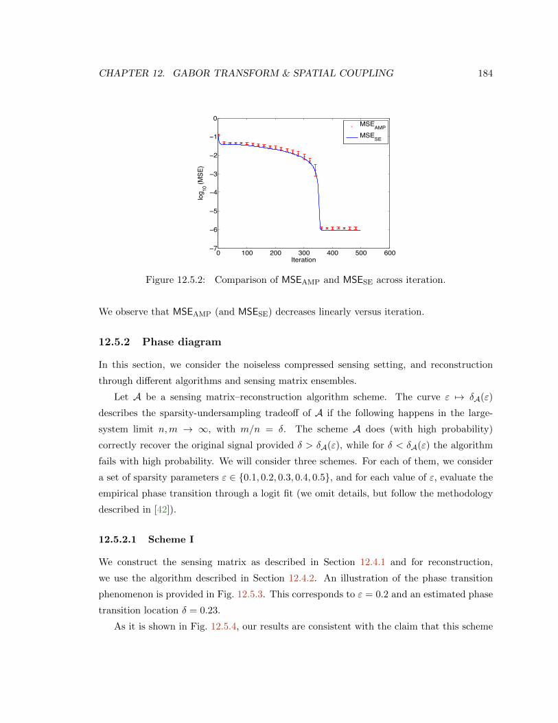
CHAPTER 12. GABOR TRANSFORM & SPATIAL COUPLING 184
0 100 200 300 400 500 600−7
−6
−5
−4
−3
−2
−1
0
Iteration
log 10
(MSE
)
MSEAMPMSESE
Figure 12.5.2: Comparison of MSEAMP and MSESE across iteration.
We observe that MSEAMP (and MSESE) decreases linearly versus iteration.
12.5.2 Phase diagram
In this section, we consider the noiseless compressed sensing setting, and reconstruction
through different algorithms and sensing matrix ensembles.
Let A be a sensing matrix–reconstruction algorithm scheme. The curve ε 7→ δA(ε)
describes the sparsity-undersampling tradeoff of A if the following happens in the large-
system limit n,m → ∞, with m/n = δ. The scheme A does (with high probability)
correctly recover the original signal provided δ > δA(ε), while for δ < δA(ε) the algorithm
fails with high probability. We will consider three schemes. For each of them, we consider
a set of sparsity parameters ε ∈ 0.1, 0.2, 0.3, 0.4, 0.5, and for each value of ε, evaluate the
empirical phase transition through a logit fit (we omit details, but follow the methodology
described in [42]).
12.5.2.1 Scheme I
We construct the sensing matrix as described in Section 12.4.1 and for reconstruction,
we use the algorithm described in Section 12.4.2. An illustration of the phase transition
phenomenon is provided in Fig. 12.5.3. This corresponds to ε = 0.2 and an estimated phase
transition location δ = 0.23.
As it is shown in Fig. 12.5.4, our results are consistent with the claim that this scheme

CHAPTER 12. GABOR TRANSFORM & SPATIAL COUPLING 185
0 0.1 0.2 0.3 0.4 0.50
0.2
0.4
0.6
0.8
1
Succ
ess
Rat
e
δ
EmpiricalLogit fit
Figure 12.5.3: Phase transition diagram for Scheme I, and ε = 0.2.
achieves successful reconstruction at rates close to the information theoretic lower bound
δ > d(pX
) = ε. (We indeed expect the gap to decrease further by taking larger values of
`, n.)
12.5.2.2 Scheme II
The sensing matrix AF is obtained by choosing m rows of the Fourier matrix F at random.
In time domain, this corresponds to sampling at m random time instants as in [23]. Recon-
struction is done via AMP algorithm with posterior expectation as the denoiser η. More
specifically, through the following iterative procedure.
xt+1 = ηt(xt +A∗rt) ,
rt = y −Axt +1
δrt−1〈∂ηt−1〉+
1
δrt−1〈∂ηt−1〉 .
(12.5.5)
Here ηt(v) = (ηt(v1), . . . , ηt(vn)), where ηt(vi) = EX|X + φ1/2t Z = vi and Z ∼ NC(0, 1).
Also ∂ηt,i ≡ ∂ηt(xti + (A∗rt)i), ∂ηt,i ≡ ∂ηt(x
ti + (A∗rt)i) and for a vector u ∈ Rn, 〈u〉 =
n−1∑n
i=1 ui.
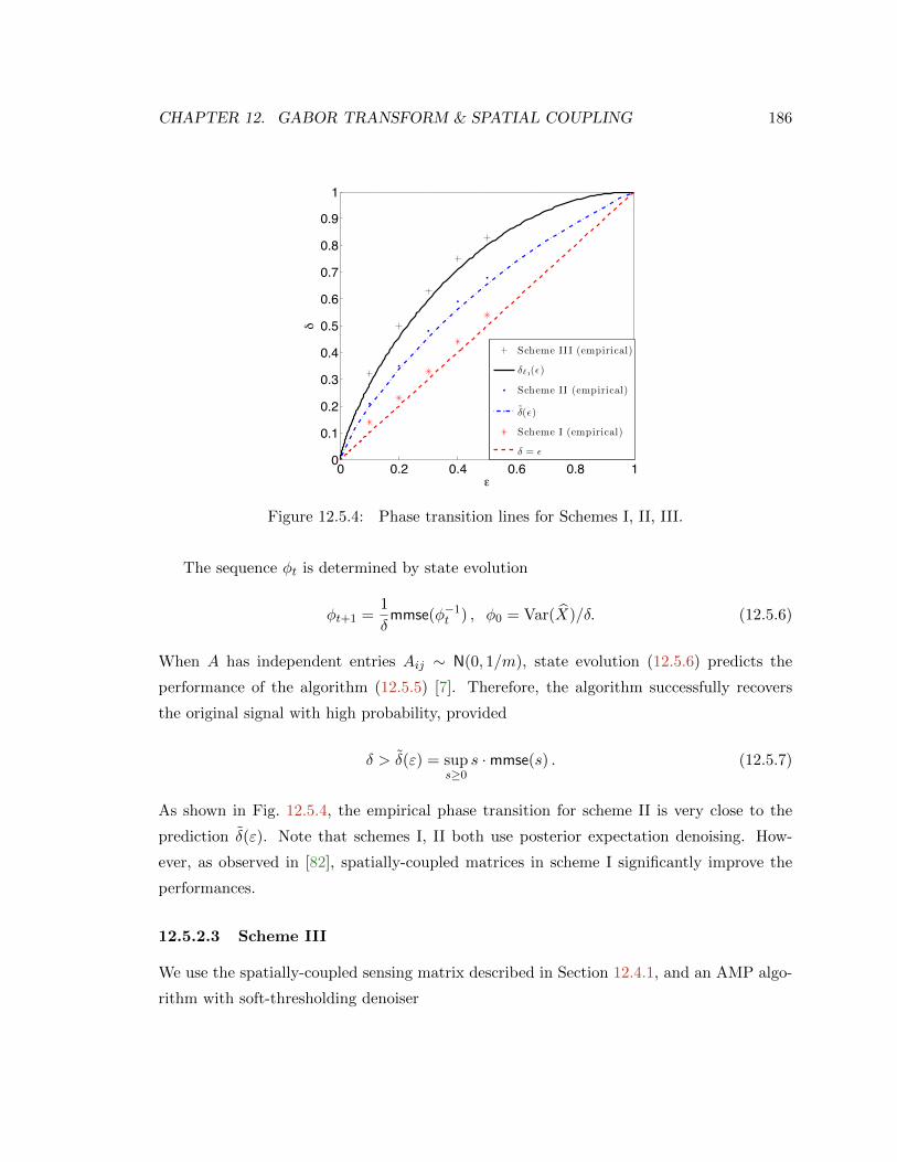
CHAPTER 12. GABOR TRANSFORM & SPATIAL COUPLING 186
0 0.2 0.4 0.6 0.8 10
0.1
0.2
0.3
0.4
0.5
0.6
0.7
0.8
0.9
1
ε
δ
Scheme II I (empirical)
!!1(")
Scheme II (empirical)
!(")
Scheme I (empirical)
! = "
Figure 12.5.4: Phase transition lines for Schemes I, II, III.
The sequence φt is determined by state evolution
φt+1 =1
δmmse(φ−1
t ) , φ0 = Var(X)/δ. (12.5.6)
When A has independent entries Aij ∼ N(0, 1/m), state evolution (12.5.6) predicts the
performance of the algorithm (12.5.5) [7]. Therefore, the algorithm successfully recovers
the original signal with high probability, provided
δ > δ(ε) = sups≥0
s ·mmse(s) . (12.5.7)
As shown in Fig. 12.5.4, the empirical phase transition for scheme II is very close to the
prediction δ(ε). Note that schemes I, II both use posterior expectation denoising. How-
ever, as observed in [82], spatially-coupled matrices in scheme I significantly improve the
performances.
12.5.2.3 Scheme III
We use the spatially-coupled sensing matrix described in Section 12.4.1, and an AMP algo-
rithm with soft-thresholding denoiser

CHAPTER 12. GABOR TRANSFORM & SPATIAL COUPLING 187
ηST (z; θ) =(
1− θ
|z|
)+z . (12.5.8)
The algorithm is defined as in Eq. (12.4.5), except that the soft-thresholding denoiser is
used in lieu of the posterior expectation. Formally, let ηt(v) = (ηt,1(v1), · · · , ηt,n(vn)) with
ηt,i(vi) = ηST (vi, α∗(ε)s
−1/2i ), si =
∑a∈[m]
Waiφa(t)−1, (12.5.9)
and the sequence of profiles φ(t)t≥0 is given by the following recursion.
φa(t+ 1) =∑i∈[n]
Wai E|ηt,i(X + s−1/2i Z;α∗s
−1/2i )− X|2.
Finally α∗ = α∗(ε) is tuned to optimize the phase transition boundary.
This is in fact a generalization of the complex AMP (CAMP) algorithm that was de-
veloped in [91] for unstructured matrices. CAMP strives to solve the standard convex
relaxation
minimize ‖x‖1
subject to AFx = y ,
where we recall ‖x‖1 ≡∑
ω∈Ωn|x(ω)|. For a given ε, we denote by δ`1(ε) the phase transition
location for `1 minimization, when sensing matrices with i.i.d. entries are used. This
coincides with the one of CAMP with optimally tuned α = α∗(ε) [146, 91].
The empirical phase transition of Scheme III is shown in Fig. 12.5.4. The results are
consistent with the claim that the phase boundary coincides with δ`1 . In other words,
spatially-coupled sensing matrix does not improve the performances under `1 reconstruc-
tion (or under AMP with soft-thresholding denoiser). This agrees with earlier findings by
Krzakala et al. for Gaussian matrices ([82], and private communications). This can be
inferred from the the state evolution map. For AMP with posterior expectation denoiser,
and for ε < δ < δ(ε), the state evolution map has two stable fixed points; one of order σ2,
and one much larger. Spatial coupling makes the algorithm converge to the ‘right’ fixed
point. However, the state evolution map corresponding to the soft-thresholding denoiser
is concave and has only one stable fixed point, much larger than σ2. Therefore, spatial
coupling is not helpful in this setting.

Appendix A
Supplement to Chapter 2
A.1 Proof of Lemma 2.4.1
Let Ci(µ) be the optimal value of the optimization problem (2.3.11). We claim that
Ci(µ) ≥ (1− µ)2
Σii
. (A.1.1)
To prove this claim notice that the constraint implies (by considering its i-th component):
1− 〈ei, Σm〉 ≤ µ .
Therefore if m is feasible and c ≥ 0, then
〈m, Σm〉 ≥ 〈m, Σm〉+ c(1− µ)− c〈ei, Σm〉 ≥ minm
〈m, Σm〉+ c(1− µ)− c〈ei, Σm〉
.
Minimizing over all feasible m gives
Ci(µ) ≥ minm
〈m, Σm〉+ c(1− µ)− c〈ei, Σm〉
. (A.1.2)
The minimum over m is achieved at m = cei/2. Plugging in for m, we get
Ci(µ) ≥ c(1− µ)− c2
4Σii (A.1.3)
188

APPENDIX A. SUPPLEMENT TO CHAPTER 2 189
Optimizing this bound over c, we obtain the claim (A.1.1), with the optimal choice being
c = 2(1− µ)/Σii.
A.2 Proof of Lemma 2.4.3
Let En = En(φ0, s0,K) be the event defined as per Theorem 2.3.4.(a). In particular, we take
φ0 =√Cmin/2, and K ≥ 1 + 20κ2
√(log p)/n.1 Further note that we can assume without
loss of generality n ≥ ν0 s0 log(p/s0), since s0 = o(√n/ log p). Fixing ε > 0, we have
P(∣∣∣ σσ− 1∣∣∣ ≥ ε) ≤ sup
X∈EnP(∣∣∣ σσ− 1∣∣∣ ≥ ε ∣∣∣X)+ P
(X 6∈ En
)≤ sup
X∈EnP(∣∣∣ σσ− 1∣∣∣ ≥ ε ∣∣∣X)+ 4 e−c1n ,
where c1 > 0 is a constant defined as per Theorem 2.3.4.(a).
We are therefore left with the task of bounding the first term in the last expression
above, uniformly over θ0 ∈ Rp, ‖θ0‖0 ≤ s0. For X ∈ En, we apply the result of [124,
Theorem 1]. More precisely, using the notations of [124], with λ0 = λ, ξ = 3, T = supp(θ0),
κ(ξ, T ) ≥ φ0, we have η∗(λ, ξ) ≤ 4s0λ2/φ2
0. Further, let σ∗ be the oracle estimator of σ
introduced there. If ‖XTW/(nσ∗)‖∞ ≤ λ/4, using Eq. (13) in [124], we obtain
∣∣∣ σσ∗− 1∣∣∣ ≤ 2
√s0λ
σ∗φ0≤ ε
2, (A.2.1)
where the last inequality follows for all n large enough since s0 = o(√n/ log p).
Hence
supX∈En
P(∣∣∣ σσ− 1∣∣∣ ≥ ε ∣∣∣X) ≤ sup
X∈EnP(‖XTW/n‖∞ > λ/4
∣∣∣X)+ supX∈En
P(∣∣∣σ∗σ− 1∣∣∣ ≥ ε
10
∣∣∣X) ,(A.2.2)
where we note that the right hand side is independent of θ0. The first term vanishes as
n → ∞ by a standard tail bound on the supremum of p Gaussian random variables. The
second term also vanishes because it is controlled by the tail of a chi-squared random variable
(see [124]).
1 For instance K = 1.1 will work for all n large enough since (s0 log p)2/n → 0, with s0 ≥ 1, byassumption.

APPENDIX A. SUPPLEMENT TO CHAPTER 2 190
A.3 Proof of Lemma 6.1.3
Write
Zi =1√n
n∑j=1
ξj with ξj ≡mTi XjWj
σ[mTi Σmi]1/2
.
Conditional on X, the summands ξj are zero mean and independent. Further,∑n
j=1 E(ξ2j |X) =
n. We next prove the Lindenberg condition as per Eq. (2.4.11). Let cn ≡ (mTi Σmi)
1/2. By
Lemma 2.4.1, we have lim infn→∞ cn ≥ c∞ > 0, almost surely. If all the optimization
problems in (2.4.12) are feasible, then |ξj | ≤ c−1n ‖Xmi‖∞‖W‖∞/σ ≤ c−1
n nβ(‖W‖∞/σ).
Hence,
limn→∞
1
n
n∑j=1
E(ξ2j I|ξj |>ε√n|X
)≤ lim
n→∞
1
n
n∑j=1
E(ξ2j I‖W‖∞/σ>εcnn1/2−β|X
)= lim
n→∞
1
n
n∑j=1
mTi XjX
Tj mi
mTi Σmi
E(W 2j I‖W‖∞>εc∞n1/2−β
)≤ lim
n→∞E(W 2
1 I|W1|>εc∞n1/2−β
)≤ c′(ε) lim
n→∞n−a(1/2−β)E|W1|2+a = 0 .
where Wj = Wj/σ and the last limit follows since β < 1/2 and a > 0.
Using Lindenberg central limit theorem, we obtain Zi|X converges weakly to standard
normal distribution, and hence, X-almost surely
limn→∞
P(Zi ≤ x|X) = Φ(x) .
What remains is to show that with high probability all the p optimization problems
in (2.4.12) are feasible. In particular, we show that Σ−1i,· is a feasible solution to the i-th
optimization problem, for i ∈ [p]. By Lemma 6.1.2, |Σ−1Σ− I|∞ ≤ µ, with high probability.
Moreover,
supj∈[p]‖Σ−1
i,· Xj‖ψ2 = supj∈[p]‖Σ−1/2
i,· Σ−1/2Xj‖ψ2
= ‖Σ−1/2i,· ‖2 sup
j∈[p]‖Σ−1/2Xj‖ψ2
= [Σ−1i,i ]1/2 sup
j∈[p]‖Σ−1/2Xj‖ψ2 = O(1) .

APPENDIX A. SUPPLEMENT TO CHAPTER 2 191
Using tail bound for sub-gaussian variables Σ−1i,· Xj and union bounding over j ∈ [n], we get
P(‖XΣ−1·,i ‖∞ > nβ) ≤ ne−cn2β
,
for some constant c > 0. Note that s0 = o(√n/ log p) and β > 1/4 imply p = eo(n
2β). Hence,
almost surely, Σ−1i,· is a feasible solution to optimization problem (2.4.12), for all i ∈ [p].

Appendix B
Supplement to Chapter 4
B.1 Effective noise variance τ 20
As stated in Theorem 4.1.4 the unbiased estimator θu can be regarded –asymptotically– as
a noisy version of θ0 with noise variance τ20 . An explicit formula for τ0 is given in [8]. For
the reader’s convenience, we explain it here using our notations.
Denote by η : R× R+ → R the soft thresholding function
η(x; a) =
x− a if x > a,
0 if − a ≤ x ≤ a
x+ a otherwise.
(B.1.1)
Further define function F : R+ × R+ → R+ as
F(τ2, a) = σ2 +1
δE[η(Θ0 + τZ; a)−Θ0]2 , (B.1.2)
where Θ0 and Z are defined as in Theorem 4.1.4. Let κmin = κmin(δ) be the unique non-
negative solution of the equation
(1 + κ2)Φ(−κ)− κφ(κ) =δ
2. (B.1.3)
The effective noise variance τ20 is obtained by solving the following two equations for κ and
192
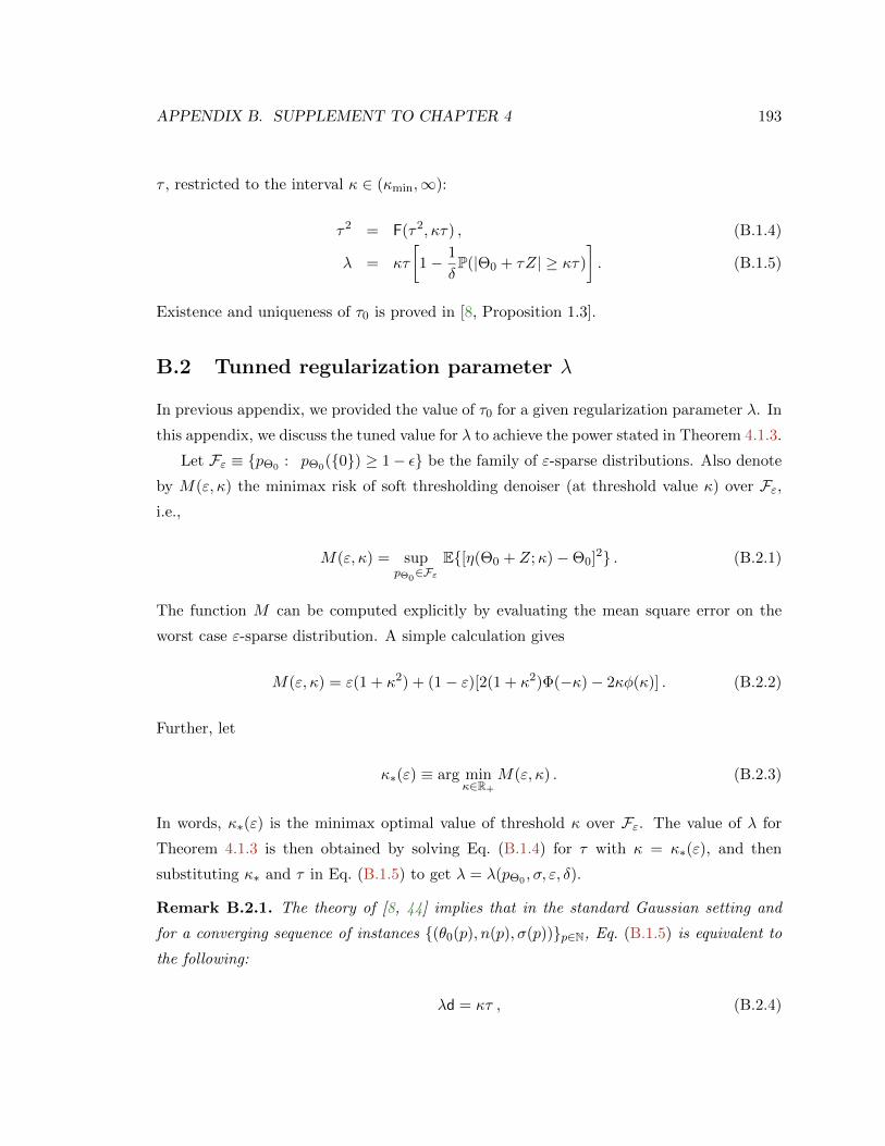
APPENDIX B. SUPPLEMENT TO CHAPTER 4 193
τ , restricted to the interval κ ∈ (κmin,∞):
τ2 = F(τ2, κτ) , (B.1.4)
λ = κτ
[1− 1
δP(|Θ0 + τZ| ≥ κτ)
]. (B.1.5)
Existence and uniqueness of τ0 is proved in [8, Proposition 1.3].
B.2 Tunned regularization parameter λ
In previous appendix, we provided the value of τ0 for a given regularization parameter λ. In
this appendix, we discuss the tuned value for λ to achieve the power stated in Theorem 4.1.3.
Let Fε ≡ pΘ0 : pΘ0(0) ≥ 1− ε be the family of ε-sparse distributions. Also denote
by M(ε, κ) the minimax risk of soft thresholding denoiser (at threshold value κ) over Fε,i.e.,
M(ε, κ) = suppΘ0∈Fε
E[η(Θ0 + Z;κ)−Θ0]2 . (B.2.1)
The function M can be computed explicitly by evaluating the mean square error on the
worst case ε-sparse distribution. A simple calculation gives
M(ε, κ) = ε(1 + κ2) + (1− ε)[2(1 + κ2)Φ(−κ)− 2κφ(κ)] . (B.2.2)
Further, let
κ∗(ε) ≡ arg minκ∈R+
M(ε, κ) . (B.2.3)
In words, κ∗(ε) is the minimax optimal value of threshold κ over Fε. The value of λ for
Theorem 4.1.3 is then obtained by solving Eq. (B.1.4) for τ with κ = κ∗(ε), and then
substituting κ∗ and τ in Eq. (B.1.5) to get λ = λ(pΘ0 , σ, ε, δ).
Remark B.2.1. The theory of [8, 44] implies that in the standard Gaussian setting and
for a converging sequence of instances (θ0(p), n(p), σ(p))p∈N, Eq. (B.1.5) is equivalent to
the following:
λd = κτ , (B.2.4)

APPENDIX B. SUPPLEMENT TO CHAPTER 4 194
where the normalization factor d is given by Eq. (4.1.2).
B.3 Replica method calculation
In this section we outline the replica calculation leading to the Claim 4.2.5. Indeed we
consider an even more general setting, where the `1 regularization is replaced by an arbitrary
separable penalty. Namely, instead of the Lasso, we consider regularized least squares
estimators of the form
θ(Y,X) = arg minθ∈Rp
1
2n‖Y −Xθ‖2 + J(θ)
, (B.3.1)
with J(θ) being a convex separable penalty function; namely for a vector θ ∈ Rp, we have
J(θ) = J1(θ1) + · · · + Jp(θp), with J` : R → R a convex function. Important instances
from this ensemble of estimators are Ridge-regression (J(θ) = λ‖θ‖2/2), and the Lasso
(J(θ) = λ‖θ‖1). The Replica Claim 4.2.5 is generalized to the present setting replacing
λ‖θ‖1 by J(θ). The only required modification concerns the definition of the factor d. We
let d be the unique positive solution of the following equation
1 =1
d+
1
nTrace
(I + dΣ−1/2∇2J(θ)Σ−1/2)−1
, (B.3.2)
where ∇2J(θ) denotes the Hessian, which is diagonal since J is separable. If J is non
differentiable, then we formally set [∇2J(θ)]ii = ∞ for all the coordinates i such that J is
non-differentiable at θi. It can be checked that this definition is well posed and yields the
previous choice for J(θ) = λ‖θ‖1.
We pass next to establishing the claim. We limit ourselves to the main steps, since
analogous calculations can be found in several earlier works [127, 63, 125]. For a general
introduction to the method and its motivation we refer to [98, 97]. Also, for the sake of
simplicity, we shall focus on characterizing the asymptotic distribution of θu, cf. Eq. (4.2.3).
The distribution of r is derived by the same approach.
Fix a sequence of instances (Σ(p), θ0(p), n(p), σ(p))p∈N. For the sake of simplicity, we
assume σ(p)2 = n(p)σ20 and n(p) = pδ (the slightly more general case σ(p)2 = n(p)[σ2
0 +o(1)]
and n(p) = p[δ+o(1)] does not require any change to the derivation given here, but is more
cumbersome notationally). Fix g : R × R × R → R a continuous function convex in its
first argument, and let g(u, y, z) ≡ maxx∈R[ux − g(x, y, z)] be its Lagrange dual. The
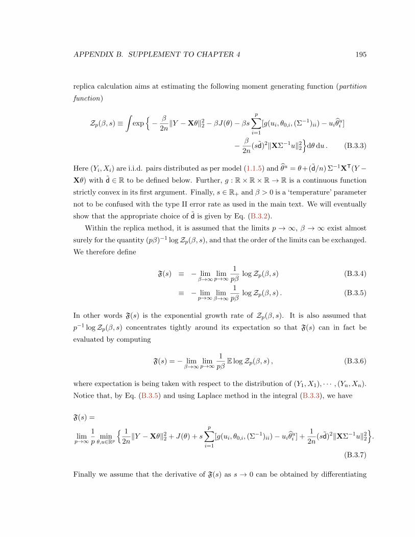
APPENDIX B. SUPPLEMENT TO CHAPTER 4 195
replica calculation aims at estimating the following moment generating function (partition
function)
Zp(β, s) ≡∫
exp− β
2n‖Y −Xθ‖22 − βJ(θ)− βs
p∑i=1
[g(ui, θ0,i, (Σ−1)ii)− uiθui ]
− β
2n(sd)2‖XΣ−1u‖22
dθ du . (B.3.3)
Here (Yi, Xi) are i.i.d. pairs distributed as per model (1.1.5) and θu = θ+(d/n) Σ−1XT(Y −Xθ) with d ∈ R to be defined below. Further, g : R× R× R→ R is a continuous function
strictly convex in its first argument. Finally, s ∈ R+ and β > 0 is a ‘temperature’ parameter
not to be confused with the type II error rate as used in the main text. We will eventually
show that the appropriate choice of d is given by Eq. (B.3.2).
Within the replica method, it is assumed that the limits p → ∞, β → ∞ exist almost
surely for the quantity (pβ)−1 logZp(β, s), and that the order of the limits can be exchanged.
We therefore define
F(s) ≡ − limβ→∞
limp→∞
1
pβlogZp(β, s) (B.3.4)
≡ − limp→∞
limβ→∞
1
pβlogZp(β, s) . (B.3.5)
In other words F(s) is the exponential growth rate of Zp(β, s). It is also assumed that
p−1 logZp(β, s) concentrates tightly around its expectation so that F(s) can in fact be
evaluated by computing
F(s) = − limβ→∞
limp→∞
1
pβE logZp(β, s) , (B.3.6)
where expectation is being taken with respect to the distribution of (Y1, X1), · · · , (Yn, Xn).
Notice that, by Eq. (B.3.5) and using Laplace method in the integral (B.3.3), we have
F(s) =
limp→∞
1
pminθ,u∈Rp
1
2n‖Y −Xθ‖22 + J(θ) + s
p∑i=1
[g(ui, θ0,i, (Σ−1)ii)− uiθui ] +
1
2n(sd)2‖XΣ−1u‖22
.
(B.3.7)
Finally we assume that the derivative of F(s) as s → 0 can be obtained by differentiating

APPENDIX B. SUPPLEMENT TO CHAPTER 4 196
inside the limit. This condition holds, for instance, if the cost function is strongly convex
at s = 0. We get
dF
ds(s = 0) = lim
p→∞
1
p
p∑i=1
minui∈R
[g(ui, θ0,i, (Σ−1)ii)− uiθui ] (B.3.8)
where θu = θ+(d/n) Σ−1XT(Y −Xθ) and θ is the minimizer of the regularized least squares
as per Eq. (B.3.1). Since, by duality g(x, y, z) ≡ maxu∈R[ux− g(u, y, z)], we get
dF
ds(s = 0) = − limp→∞
1p
∑pi=1 g(θui , θ0,i, (Σ
−1)ii) . (B.3.9)
Hence, by computing F(s) using Eq. (B.3.6) for a complete set of functions g, we get access
to the corresponding limit quantities (B.3.9) and hence, via standard weak convergence
arguments, to the joint empirical distribution of the triple (θui , θ0,i, (Σ−1)ii), cf. Eq. (4.2.4).
In order to carry out the calculation of F(s), we begin by rewriting the partition function
(B.3.3) in a more convenient form. Using the definition of θu and after a simple manipulation
Zp(β, s) =∫exp
− β
2n‖Y −X(θ + sdΣ−1u)‖22 − βJ(θ) + βs〈u, θ〉 − β s
p∑i=1
g(ui, θ0,i, (Σ−1)ii)
dθ du .
(B.3.10)
Define the measure ν(dθ) over θ ∈ Rp as follows
ν(dθ) =
∫exp
− βJ(θ − sdΣ−1u) + βs〈θ − sdΣ−1u, u〉 − βs
p∑i=1
g(ui, θ0,i, (Σ−1)ii)
du .
(B.3.11)
Using this definition and with the change of variable θ′ = θ + sdΣ−1u, we can rewrite

APPENDIX B. SUPPLEMENT TO CHAPTER 4 197
Eq. (B.3.10) as
Zp(β, s) ≡∫
exp− β
2n‖Y −Xθ‖22
ν(dθ)
=
∫exp
i
√β
n〈z, Y −Xθ〉
ν(dθ) γn(dz)
=
∫exp
i
√β
n〈W, z〉+ i
√β
n〈z,X(θ0 − θ)〉
ν(dθ) γ(dz) , (B.3.12)
where γn(dz) denotes the standard Gaussian measure on Rn:
γn(dz) ≡ (2π)−n2 exp
(− ‖z‖
22
2
)dz.
The replica method aims at computing the expected log-partition function, cf. Eq. (B.3.6)
using the identity
E logZp(β, s) =d
dk
∣∣∣∣k=0
logEZp(β, s)k
. (B.3.13)
This formula would require computing fractional moments of Zp as k → 0. The replica
method consists in a prescription that allows to compute a formal expression for the k
integer, and then extrapolate it as k → 0. Crucially, the limit k → 0 is inverted with the
one p→∞:
limp→∞
1
pE logZp(β, s) =
d
dk
∣∣∣∣k=0
limp→∞
1
plogE
Zp(β, s)k
. (B.3.14)
In order to represent Zp(β, s)k, we use the identity
(∫f(x) ρ(dx)
)k=
∫f(x1)f(x2) · · · f(xk) ρ(dx1) · · · ρ(dxk) . (B.3.15)
In order to apply this formula to Eq. (B.3.12), we let, with a slight abuse of notation,
νk(dθ) ≡ ν(dθ1) × ν(dθ2) × · · · × ν(dθk) be a measure over (Rp)k, with θ1, . . . , θk ∈ Rp.Analogously γkn(dz) ≡ γn(dz1)× γn(dz2)× · · · × γn(dzk), with z1, . . . , zk ∈ Rn. With these

APPENDIX B. SUPPLEMENT TO CHAPTER 4 198
notations, we have
EZp(β, s)k =
∫E exp
i
√β
n〈W,
k∑a=1
za〉+ i
√β
n〈X,
k∑a=1
za(θ0 − θa)T〉νk(dθ) γkn(dz) .
(B.3.16)
In the above expression E denotes expectation with respect to the noise vector W , and
the design matrix X. Further, we used 〈 · , · 〉 to denote matrix scalar product as well:
〈A,B〉 ≡ Trace(ATB).
At this point we can take the expectation with respect to W , X. We use the fact that,
for any M ∈ Rn×p, u ∈ Rn
E
exp(i〈W,u〉
)= exp
− 1
2nσ2
0 ‖u‖22,
E
exp(i〈M,X〉
)= exp
− 1
2〈M,MΣ〉
,
(B.3.17)
Using these identities in Eq. (B.3.16), we obtain
EZkp =∫exp
− 1
2βσ2
0
k∑a=1
‖za‖22 −β
2n
k∑a,b=1
〈za, zb〉 〈(θa − θ0),Σ(θb − θ0)〉νk(dθ) γkn(dz) .
(B.3.18)
We next use the identity
e−xy =1
2πi
∫(−i∞,i∞)
∫(−∞,∞)
e−ζq+ζx−qy dζ dq , (B.3.19)
where the integral is over ζ ∈ (−i∞, i∞) (imaginary axis) and q ∈ (−∞,∞). We apply
this identity to Eq. (B.3.18), and introduce integration variables Q ≡ (Qab)1≤a,b≤k and
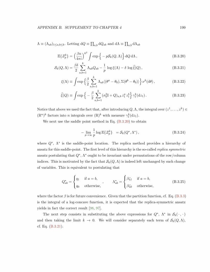
APPENDIX B. SUPPLEMENT TO CHAPTER 4 199
Λ ≡ (Λab)1≤a,b≤k. Letting dQ ≡∏a,b dQab and dΛ ≡
∏a,b dΛab
EZkp =( βn
4πi
)k2 ∫exp
− pSk(Q,Λ)
dQdΛ , (B.3.20)
Sk(Q,Λ) =βδ
2
k∑a,b=1
ΛabQab −1
plog ξ(Λ)− δ log ξ(Q) , (B.3.21)
ξ(Λ) ≡∫
expβ
2
k∑a,b=1
Λab〈(θa − θ0),Σ(θb − θ0)〉νk(dθ) , (B.3.22)
ξ(Q) ≡∫
exp− β
2
k∑a,b=1
(σ20I +Q)a,b z
a1 z
b1
γk1 (dz1) . (B.3.23)
Notice that above we used the fact that, after introducingQ,Λ, the integral over (z1, . . . , zk) ∈(Rn)k factors into n integrals over (R)k with measure γk1 (dz1).
We next use the saddle point method in Eq. (B.3.20) to obtain
− limp→∞
1
plogEZkp = Sk(Q∗,Λ∗) , (B.3.24)
where Q∗, Λ∗ is the saddle-point location. The replica method provides a hierarchy of
ansatz for this saddle-point. The first level of this hierarchy is the so-called replica symmetric
ansatz postulating that Q∗, Λ∗ ought to be invariant under permutations of the row/column
indices. This is motivated by the fact that Sk(Q,Λ) is indeed left unchanged by such change
of variables. This is equivalent to postulating that
Q∗ab =
q1 if a = b,
q0 otherwise,, Λ∗ab =
βζ1 if a = b,
βζ0 otherwise,(B.3.25)
where the factor β is for future convenience. Given that the partition function, cf. Eq. (B.3.3)
is the integral of a log-concave function, it is expected that the replica-symmetric ansatz
yields in fact the correct result [98, 97].
The next step consists in substituting the above expressions for Q∗, Λ∗ in Sk( · , · )and then taking the limit k → 0. We will consider separately each term of Sk(Q,Λ),
cf. Eq. (B.3.21).

APPENDIX B. SUPPLEMENT TO CHAPTER 4 200
Let us begin with the first term
k∑a,b=1
Λ∗abQ∗ab = k βζ1q1 + k(k − 1)βζ0q0 . (B.3.26)
Hence
limk→0
βδ
2k
k∑a,b=1
Λ∗abQ∗ab =
β2δ
2(ζ1q1 − ζ0q0) . (B.3.27)
Let us consider ξ(Q∗). We have
log ξ(Q∗) = −1
2log Det(I + βσ2I + βQ∗) (B.3.28)
= −k − 1
2log(1 + β(q1 − q0)
)− 1
2log(1 + β(q1 − q0) + βk(σ2 + q0)
). (B.3.29)
In the limit k → 0 we thus obtain
limk→0
1
k(−δ) log ξ(Q∗) =
δ
2log(1 + β(q1 − q0)
)+δ
2
β(σ2 + q0)
1 + β(q1 − q0). (B.3.30)
Finally, introducing the notation ‖v‖2Σ ≡ 〈v,Σv〉, we have
ξ(Λ∗) ≡∫
expβ2
2(ζ1 − ζ0)
k∑a=1
‖θa − θ0‖2Σ +β2ζ0
2
k∑a,b=1
〈(θa − θ0),Σ(θb − θ0)〉νk(dθ) ,
= E∫
expβ2
2(ζ1 − ζ0)
k∑a=1
‖θa − θ0‖2Σ + β√ζ0
k∑a=1
〈z,Σ1/2(θa − θ0)〉νk(dθ) ,
(B.3.31)
where expectation is with respect to z ∼ N(0, Ip×p). Notice that, given z ∈ Rp, the integrals
over θ1, θ2, . . . , θk factorize, whence
ξ(Λ∗) = E
[∫exp
β2
2(ζ1 − ζ0)‖θ − θ0‖2Σ + β
√ζ0〈z,Σ1/2(θ − θ0)〉
ν(dθ)
]k. (B.3.32)

APPENDIX B. SUPPLEMENT TO CHAPTER 4 201
Therefore
limk→0
(−1)
pklog ξ(Λ∗) =
− 1
pE
log
[∫exp
β2
2(ζ1 − ζ0)‖θ − θ0‖2Σ + β
√ζ0〈z,Σ1/2(θ − θ0)〉
ν(dθ)
].
(B.3.33)
Putting Eqs. (B.3.27), (B.3.30), and (B.3.33) together we obtain
− limp→∞
1
pβE logZp = lim
k→0
1
kβSk(Q∗,Λ∗)
=βδ
2(ζ1q1 − ζ0q0) +
δ
2βlog(1 + β(q1 − q0)
)+δ
2
σ2 + q0
1 + β(q1 − q0)
− limp→∞
1
pβE
log
[∫exp
β2
2(ζ1 − ζ0)‖θ − θ0‖2Σ
+ β√ζ0〈z,Σ1/2(θ − θ0)〉
ν(dθ)
]. (B.3.34)
We can next take the limit β → ∞. In doing this, one has to be careful with respect
to the behavior of the saddle point parameters q0, q1, ζ0, ζ1. A careful analysis (omitted
here) shows that q0, q1 have the same limit, denoted here by q0, and ζ0, ζ1 have the same
limit, denoted by ζ0. Moreover q1 − q0 = (q/β) + o(β−1) and ζ1 − ζ0 = (−ζ/β) + o(β−1).
Substituting in the above expression, and using Eq. (B.3.6), we get
F(s) =δ
2(ζ0q − ζq0) +
δ
2
q0 + σ2
1 + q
+ limp→∞
1
pE minθ∈Rp
ζ2‖θ − θ0‖2Σ −
√ζ0〈z,Σ1/2(θ − θ0)〉+
˜J(θ; s)
, (B.3.35)
˜J(θ; s) = min
u∈Rp
J(θ − sdΣ−1u)− s〈θ − sdΣ−1u, u〉+ s
p∑i=1
g(ui, θ0,i, (Σ−1)ii)
. (B.3.36)

APPENDIX B. SUPPLEMENT TO CHAPTER 4 202
After the change of variable θ − sdΣ−1u→ θ, this reads
F(s) =δ
2(ζ0q − ζq0) +
δ
2
q0 + σ20
1 + q− ζ0
2ζ
+ limp→∞
1
pE minθ,u∈Rp
ζ2
∥∥∥θ − θ0 −√ζ0
ζΣ−1/2z + sdΣ−1u
∥∥∥2
Σ+ J(θ, u; s)
,
J(θ, u; s) = J(θ)− s〈θ, u〉+ s
p∑i=1
g(ui, θ0,i, (Σ−1)ii) .
Finally, we must set ζ, ζ0 and q, q0 to their saddle point values. We start by using the
stationarity conditions with respect to q, q0:
∂F
∂q(s) =
δ
2ζ0 −
δ
2
q0 + σ20
(1 + q)2, (B.3.37)
∂F
∂q0(s) = −δ
2ζ +
δ
2
1
1 + q. (B.3.38)
We use these to eliminate q and q0. Renaming ζ0 = ζ2τ2, we get our final expression for
F(s):
F(s) =− 1
2(1− δ)ζτ2 − δ
2ζ2τ2 +
δ
2σ2
0ζ
+ limp→∞
1
pE minθ,u∈Rp
ζ2
∥∥∥θ − θ0 − τΣ−1/2z + sdΣ−1u∥∥∥2
Σ+ J(θ, u; s)
, (B.3.39)
with
J(θ, u; s) = J(θ)− s〈θ, u〉+ s
p∑i=1
g(ui, θ0,i, (Σ−1)ii) . (B.3.40)
Here it is understood that ζ and τ2 are to be set to their saddle point values.
We are interested in the derivative of F(s) with respect to s, cf. Eq. (B.3.9). Consider
first the case s = 0. Using the assumption E(p)(a, b)→ E(a, b), cf. Eq. (4.2.9), we get
F(s = 0) = −1
2(1− δ)ζτ2 − δ
2ζ2τ2 +
δ
2σ2
0ζ + E(τ2, ζ) . (B.3.41)

APPENDIX B. SUPPLEMENT TO CHAPTER 4 203
The values of ζ, τ2 are obtained by setting to zero the partial derivatives
∂F
∂ζ(s = 0) = −1
2(1− δ)τ2 − δζτ2 +
δ
2σ2
0 +∂E
∂ζ(τ2, ζ) , (B.3.42)
∂F
∂τ2(s = 0) = −1
2(1− δ)ζ − δ
2ζ2 +
∂E
∂τ2(τ2, ζ) , (B.3.43)
Define, as in the statement of the Replica Claim
E1(a, b) ≡ limp→∞
1
pE∥∥ηb(θ0 +
√aΣ−1/2z)− θ0
∥∥2
Σ
, (B.3.44)
E2(a, b) ≡ limp→∞
1
pE
div ηb(θ0 +√aΣ−1/2z)
= lim
p→∞
1
pτE〈ηb(θ0 +
√aΣ−1/2z),Σ1/2z〉
, (B.3.45)
where the last identity follows by integration by parts. These limits exist by the assumption
that ∇E(p)(a, b)→ ∇E(a, b). In particular
∂E
∂ζ(τ2, ζ) =
1
2E1(τ2, ζ)− τ2 E2(τ2, ζ) +
1
2τ2 , (B.3.46)
∂E
∂τ2(τ2, ζ) = −ζ
2E2(τ2, ζ) +
1
2ζ . (B.3.47)
Substituting these expressions in Eqs. (B.3.42), (B.3.43), and simplifying, we conclude that
the derivatives vanish if and only if ζ, τ2 satisfy the following equations
τ2 = σ20 +
1
δE1(τ2, ζ) , (B.3.48)
ζ = 1− 1
δE2(τ2, ζ) . (B.3.49)
The solution of these equations is expected to be unique for J convex and σ20 > 0.
Next consider the derivative of F(s) with respect to s, which is our main object of
interest, cf. Eq. (B.3.9). By differentiating Eq. (B.3.39) and inverting the order of derivative
and limit, we get
dF
ds(s = 0) = lim
p→∞
1
pE minu∈Rp
ζd〈u, θ − θ0 − τΣ−1/2z〉 − 〈θ, u〉+
p∑i=1
g(ui, θ0,i, (Σ−1)ii)
,
where θ is the minimizer at s = 0, i.e., θ = ηζ(θ0 + τΣ−1/2z), and ζ, τ2 solve Eqs. (B.3.48),

APPENDIX B. SUPPLEMENT TO CHAPTER 4 204
(B.3.49). At this point we choose d = 1/ζ. Minimizing over u (recall that g(x, y, z) =
maxu∈R[ux− g(u, y, z)]), we get
dF
ds(s = 0) = − lim
p→∞
1
pE g(θ0,i + τ(Σ−1/2z)i, θ0,i, (Σ
−1)ii) . (B.3.50)
Comparing with Eq. (B.3.9), this proves the claim that the standard distributional limit
does indeed hold.
Notice that τ2 is given by Eq. (B.3.48) that, for d = 1/ζ coincides with the claimed
Eq. (4.2.12). Finally consider the scale parameter d = d(p) defined by Eq. (B.3.2). We
claim that
limp→∞
d(p) = d =1
ζ. (B.3.51)
Consider, for the sake of simplicity, the case that J is differentiable and strictly convex (the
general case can be obtained as a limit). Then the minimum condition of the proximal
operator (4.2.10) reads
θ = ηb(Y ) ⇔ bΣ(Y − θ) = ∇J(θ) . (B.3.52)
Differentiating with respect to θ, and denoting by Dηb the Jacobian of ηb, we get Dηb(Y ) =
(I + b−1Σ−1∇2J(θ))−1 and hence
E2(a, b) = limp→∞
1
pETrace
(1 + b−1Σ−1/2∇2J(θ)Σ−1/2)−1
, (B.3.53)
θ ≡ ηb(θ0 +√aΣ−1/2 z) . (B.3.54)
Hence, combining Eqs. (B.3.49) and (B.3.53) implies that d = ζ−1 satisfies
1 =1
d+ limp→∞
1
nETrace
(1 + dΣ−1/2∇2J(θ)Σ−1/2)−1
, (B.3.55)
θ ≡ η1/d(θ0 + τ Σ−1/2 z) . (B.3.56)
The claim (B.3.51) follows by comparing this with Eq. (B.3.2), and noting that, by the
above θ is indeed asymptotically distributed as the estimator (B.3.1).

Appendix C
Supplement to Chapter 7
C.1 Dependence of the algorithm on the prior pX
In this appendix we briefly discuss the impact of a wrong estimation of the prior pX on the
AMP algorithm. Namely, suppose that instead of the true prior pX , we have an approxima-
tion of pX denoted by pX
. The only change in the algorithm is in the posterior expectation
denoiser. That is to say, the denoiser η in Eq. (7.1.3) will be replaced by a new denoiser η.
We will quantify the discrepancy between pX and pX
through their Kolmogorov-Smirnov
distance DKS(pX , pX). Denoting by FX(z) = pX((−∞, z]) and FX
(z) = pX
((−∞, z]) the
corresponding distribution functions, we have
DKS(pX , pX) = supz∈R
∣∣FX(z)− FX
(z)∣∣ .
The next lemma establishes a bound on the pointwise distance between η and η in terms
of DKS(pX , pX).
Note that state evolution (8.2.4) applies also to the algorithm with the mismatched
denoiser, provided the mmse( · ) function is replaced by the mean square error for the non-
optimal denoiser η. Hence the bound on |η(y) − η(y)| given below can be translated into
a bound on the performance of AMP with the mismatched prior. A full study of this
issue goes beyond the scope of this dissertation and will be the object of a forthcoming
publication.
For the sake of simplicity we shall assume that pX , pX have bounded supports. The
general case requires a more careful consideration.
205

APPENDIX C. SUPPLEMENT TO CHAPTER 7 206
Lemma C.1.1. Let η : R → R be the Bayes optimal estimator for estimating X ∼ pX in
Gaussian noise η(y) = E(X|X + Z = y), with Z ∼ N(0, 1). Define denoiser η similarly,
with respect to pX
. Assume that pX is supported in [−M,M ]. Then for any pX
supported
in [−M,M ], we have
|η(y)− η(y)| ≤ M(15 + 10M |y|)Ee−X2/2
DKS(pX , pX) e2M |y| .
Proof. Throughout the proof we let ∆ ≡ DKS(pX , pX), and ∆1 ≡ Ee−X2/2.Let γ(z) = exp(−z2/2)/
√2π be the Gaussian density. We then have η(y) = EXγ(X −
y)/Eγ(X−y). Let pW be the probability measure with Radon-Nikodym derivative with
respect to pX given by
dpWdpX
(x) =e−x
2/2
Ee−X2/2.
We define pW
analogously from the measure pX
and let W, W be two random variables with
law pW and pW
, respectively. We then have
η(y) =EWeyW EeyW
. (C.1.1)
Letting FW , FW
denote the corresponding distribution functions, we have
FW (x) =
∫ x
−∞dpW (w) =
∫ x−∞ e
−z2/2 dpX(z)
Ee−X2/2=e−x
2/2FX(x) +∫ x−∞ ze
−z2/2FX(z) dz∫∞−∞ ze
−z2/2FX(z) dz.
Letting NW (x) be the numerator in this expression, we have
∣∣NW (x)−NW
(x)∣∣ ≤ ∣∣FX(x)− F
X(x)∣∣+
∫ x
−∞|z| e−z2/2
∣∣FX(z)− FX
(z)∣∣dz ≤ 3∆ .
Proceeding analogously for the denominator, we have
∣∣Ee−X2/2 − Ee−X2/2∣∣ ≤ ∫ ∞
−∞|z| e−z2/2
∣∣FX(z)− FX
(z)∣∣dz ≤ 2∆ .
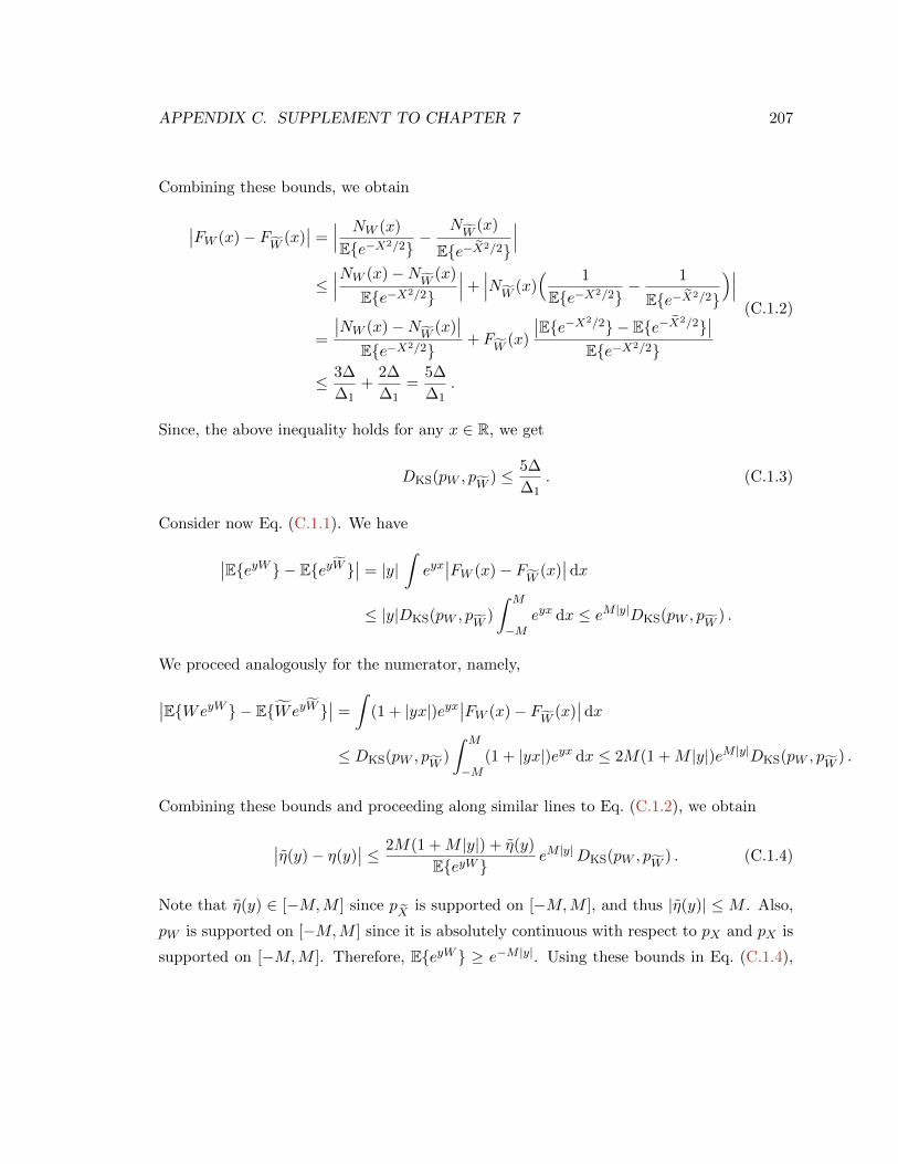
APPENDIX C. SUPPLEMENT TO CHAPTER 7 207
Combining these bounds, we obtain
∣∣FW (x)− FW
(x)∣∣ =
∣∣∣ NW (x)
Ee−X2/2−
NW
(x)
Ee−X2/2
∣∣∣≤∣∣∣NW (x)−N
W(x)
Ee−X2/2
∣∣∣+∣∣∣NW
(x)( 1
Ee−X2/2− 1
Ee−X2/2
)∣∣∣=
∣∣NW (x)−NW
(x)∣∣
Ee−X2/2+ F
W(x)
∣∣Ee−X2/2 − Ee−X2/2∣∣
Ee−X2/2
≤ 3∆
∆1+
2∆
∆1=
5∆
∆1.
(C.1.2)
Since, the above inequality holds for any x ∈ R, we get
DKS(pW , pW ) ≤ 5∆
∆1. (C.1.3)
Consider now Eq. (C.1.1). We have
∣∣EeyW − EeyW ∣∣ = |y|
∫eyx∣∣FW (x)− F
W(x)∣∣dx
≤ |y|DKS(pW , pW )
∫ M
−Meyx dx ≤ eM |y|DKS(pW , pW ) .
We proceed analogously for the numerator, namely,
∣∣EWeyW − EWeyW ∣∣ =
∫(1 + |yx|)eyx
∣∣FW (x)− FW
(x)∣∣dx
≤ DKS(pW , pW )
∫ M
−M(1 + |yx|)eyx dx ≤ 2M(1 +M |y|)eM |y|DKS(pW , pW ) .
Combining these bounds and proceeding along similar lines to Eq. (C.1.2), we obtain
∣∣η(y)− η(y)∣∣ ≤ 2M(1 +M |y|) + η(y)
EeyW eM |y|DKS(pW , pW ) . (C.1.4)
Note that η(y) ∈ [−M,M ] since pX
is supported on [−M,M ], and thus |η(y)| ≤ M . Also,
pW is supported on [−M,M ] since it is absolutely continuous with respect to pX and pX is
supported on [−M,M ]. Therefore, EeyW ≥ e−M |y|. Using these bounds in Eq. (C.1.4),

APPENDIX C. SUPPLEMENT TO CHAPTER 7 208
we obtain
∣∣η(y)− η(y)∣∣ ≤M(3 + 2M |y|) e2M |y|DKS(pW , pW ) . (C.1.5)
The result follows by plugging in the bound given by Eq. (C.1.3).
C.2 Lipschitz continuity of AMP
Let xt be the Bayes optimal AMP estimation at iteration t as given by Eqs. (7.1.3), (7.1.4).
We show that for each fixed iteration number t, the mapping y → xt(y) is locally Lipschitz
continuous.
Lemma C.2.1. For any R,B > 0, t ∈ N, there exists L = L(R,B; t) < ∞ such that for
any y, y ∈ Rm with ‖y‖, ‖y‖ ≤ R, and any matrix A with ‖A‖2 ≤ B we have
‖xt(y)− xt(y)‖ ≤ L ‖y − y‖ . (C.2.1)
Note that in the statement we assume ‖A‖2 to be finite. This happens as long as the
entries of A are bounded and hence almost surely within our setting.
Also, we assume ‖y‖, ‖y‖ ≤ R for some fixed R. In other words, we prove that the
algorithm is locally Lipschitz. We can obtain an algorithm that is globally Lipschitz by
defining xt(y) via the AMP iteration for ‖y‖ ≤ R, and by an arbitrary bounded Lipschitz
extension for ‖y‖ ≥ R. Notice that ‖y‖ ≤ B‖x‖ + ‖w‖, and, by the law of large numbers,
‖x‖2 ≤ (EX2+ε)n, ‖w‖2 ≤ (σ2+ε)m with probability converging to 1. Hence, the globally
Lipschitz modification of AMP achieves the same performance as the original AMP, almost
surely. (Note that R can depend on n).
Proof (Lemma C.2.1). Suppose that we have two measurement vectors y and y. Note that
the state evolution is completely characterized in terms of prior pX and noise variance σ2,
and can be precomputed (independent of measurement vector).
Let (xt, rt) correspond to the AMP with measurement vector y and (xt, rt) correspond
to the AMP with measurement vector y. (To clarify, note that xt ≡ xt(y) and xt ≡ xt(y)).
Further define
ξt = max(‖xt − xt‖, ‖rt − rt‖, ‖y − y‖) .

APPENDIX C. SUPPLEMENT TO CHAPTER 7 209
We show that
ξt ≤ Ct(1 + ‖y‖) ξt−1 , (C.2.2)
for a constant Ct. This establishes the claim since
‖xt − xt‖ ≤ ξt ≤ CtCt−1 . . . C2 (1 + ‖y‖)t−1ξ1 = CtCt−1 . . . C2 (1 + ‖y‖)t−1‖y − y‖ ,
where the last step holds since x1i = x1
i = EX and r1 − r1 = y − y.
In order to prove Eq. (C.2.2), we need to prove the following two claims.
Claim C.2.2. For any fixed iteration number t, there exists a constant Ct, such that
‖rt‖ ≤ Ct max(‖x1‖, ‖y‖) .
Proof (Claim C.2.2). Define λt = max(‖xt+1‖, ‖rt‖, ‖y‖). Then,
‖rt‖ ≤ ‖y‖+ ‖A‖2‖xt‖+ ‖bt‖∞‖rt−1‖.
Note that A has bounded operator by assumption. Also, the posterior mean η is a smooth
function with bounded derivative. Therefore, recalling the definition of bt,
bt ≡ 1
δ
∑u∈C
Wg(i),uQt−1g(i),u〈η
′t−1〉u ,
we have ‖bt‖∞ ≤ C1,t for some constant C1,t. Hence, ‖rt‖ ≤ C2,tλt−1. Moreover,
‖xt+1‖ = ‖ηt(xt + (Qt A)∗rt)‖ ≤ C(‖xt‖+ ‖Qt A‖2‖rt‖) ≤ C3,t max(‖xt‖, ‖rt‖) ,
for some constant C3,t. In the first inequality, we used the fact that η is Lipschitz continuous.
Therefore, λt ≤ C ′tλt−1, where C ′t = max(1, C2,t, C3,t, C2,tC3,t), and
‖rt‖ ≤ λt ≤ C ′t · · ·C ′1λ0 ≤ C ′t · · ·C ′1 max(‖x1‖, ‖y‖),
with x1i = EX, for i ∈ [n].

APPENDIX C. SUPPLEMENT TO CHAPTER 7 210
Claim C.2.3. For any fixed iteration number t, there exists a constant Ct, such that
‖bt rt−1 − bt rt−1‖ ≤ Ct(1 + ‖y‖) max(‖xt−1 − xt−1‖, ‖rt−1 − rt−1‖) .
Proof (Claim C.2.3). Using triangle inequality, we have
‖bt rt−1 − bt rt−1‖ ≤ ‖(bt − bt) rt−1‖+ ‖bt (rt−1 − rt−1)‖ . (C.2.3)
Since η′ is Lipschitz continuous, we have
‖bt − bt‖ ≤ C1,t(‖xt−1 − xt−1‖+ ‖rt−1 − rt−1‖) ,
for some constant C1,t. Also, as discussed in the proof of Claim C.2.2, the Onsager terms
bt are uniformly bounded. Applying these bounds to the right hand side of Eq. (C.2.3), we
obtain
‖bt rt−1 − bt rt−1‖ ≤ C1,t (‖xt−1 − xt−1‖+ ‖rt−1 − rt−1‖) ‖rt−1‖+ C2,t ‖rt−1 − rt−1‖
≤ Ct(1 + ‖y‖) max(‖xt−1 − xt−1‖, ‖rt−1 − rt−1‖) ,
for some constants C1,t, C2,t, Ct. The last inequality here follows from the bound given in
Claim C.2.2.
Now, we are ready to prove Eq. (C.2.2). We write
‖xt − xt‖ = ‖ηt−1(xt−1 + (Qt−1 A)∗rt−1)− ηt−1(xt−1 + (Qt−1 A)∗rt−1)‖
≤ C(‖xt−1 − xt−1‖+ ‖Qt−1 A‖2‖rt−1 − rt−1‖
)≤ C1,t max(‖xt−1 − xt−1‖, ‖rt−1 − rt−1‖, ‖y − y‖) = C1,t ξt−1 , (C.2.4)
for some constant C1,t. Furthermore,
‖rt − rt‖ ≤ ‖y − y‖+ ‖A‖2‖xt − xt‖+ ‖bt rt−1 − bt rt−1‖
≤ ‖y − y‖+ ‖A‖2C1,t ξt−1 + C ′t(1 + ‖y‖) max(‖xt−1 − xt−1‖, ‖rt−1 − rt−1‖)
≤ C2,t (1 + ‖y‖) ξt−1 , (C.2.5)

APPENDIX C. SUPPLEMENT TO CHAPTER 7 211
for some constant C2,t and using Eq. (C.2.4) and Claim C.2.3 in deriving the second in-
equality. Combining Eqs. (C.2.4) and (C.2.5), we obtain
ξt ≤ max(1, C1,t, C2,t) (1 + ‖y‖) ξt−1 .

Appendix D
Supplement to Chapter 11
D.1 Proof of Lemma 11.4.2
We prove the first claim, Eq. (11.4.4). The second one follows by a similar argument. The
proof uses induction on t. It is a simple exercise to show that the induction basis (t = 1)
holds (the calculation follows the same lines as the induction step). Assuming the claim for
t, we write, for i ∈ 0, 1, . . . , L− 1
|ψi(t+ 1)− ψ(ρi; t+ 1)| =∣∣∣mmse
( ∑b∈R0
Wb−i [σ2 +1
δ
∑j∈Z
Wb−jψj(t)]−1)
−mmse(∫ `+1
−1W(z − ρi) [σ2 +
1
δ
∫RW(z − y)ψ(y; t)dy]−1dz
)∣∣∣≤∣∣∣mmse
( ∑b∈R0
Wb−i [σ2 +1
δ
∑j∈Z
Wb−jψj(t)]−1)
−mmse( ∑b∈R0
Wb−i [σ2 +1
δ
∑j∈Z
Wb−jψ(ρj; t)]−1)∣∣∣
+∣∣∣mmse
( ∑b∈R0
ρW(ρ(b− i)) [σ2 +1
δ
∑j∈Z
ρW(ρ(b− j))ψ(ρj; t)]−1)
−mmse(∫ `+1
−1W(z − ρi) [σ2 +
1
δ
∫RW(z − y)ψ(y; t)dy]−1dz
)∣∣∣.
(D.1.1)
Now, we bound the two terms on the right hand side separately. Note that the arguments
of mmse( · ) in the above terms are at most 2/σ2. Since mmse has a continuous derivative,
there exists a constant C such that | dds mmse(s)| ≤ C, for s ∈ [0, 2/σ2]. Then, considering
212

APPENDIX D. SUPPLEMENT TO CHAPTER 11 213
the first term in the upper bound (D.1.1), we have∣∣∣mmse( ∑b∈R0
Wb−i [σ2 +1
δ
∑j∈Z
Wb−jψj(t)]−1)−mmse
( ∑b∈R0
Wb−i [σ2 +1
δ
∑j∈Z
Wb−jψ(ρj; t)]−1)∣∣∣
≤ C∣∣∣ ∑b∈R0
Wb−i
([σ2 +
1
δ
∑j∈Z
Wb−jψj(t)]−1 − [σ2 +
1
δ
∑j∈Z
Wb−jψ(ρj; t)]−1)∣∣∣
≤ C
σ4
∑b∈R0
Wb−i1
δ
∣∣∣ L−1∑j=−∞
Wb−j(ψ(ρj; t)− ψj(t))∣∣∣
≤ C
δσ4
∑b∈R0
Wb−i
L−1∑j=−∞
Wb−j |ψ(ρj; t)− ψj(t)|
=C
δσ4
L−1∑j=0
( ∑b∈R0
Wb−iWb−j
)|ψ(ρj; t)− ψj(t)|
≤ C
δσ4
(∑i∈Z
W 2i
) L−1∑j=0
|ψ(ρj; t)− ψj(t)|
≤ C ′ρ
δσ4
L−1∑j=0
|ψ(ρj; t)− ψj(t)|.
(D.1.2)
Here we used∑
i∈ZW2i =
∑i∈Z ρ
2W(ρi)2 ≤ C∑|i|≤ρ−1 ρ2 ≤ Cρ (where the first inequality
follows from the fact that W is bounded).

APPENDIX D. SUPPLEMENT TO CHAPTER 11 214
To bound the second term in Eq. (D.1.1), note that∣∣∣mmse( ∑b∈R0
ρW(ρ(b− i)) [σ2 +1
δ
∑j∈Z
ρW(ρ(b− j))ψ(ρj; t)]−1)
−mmse(∫ `+1
−1W(z − ρi) [σ2 +
1
δ
∫RW(z − y)ψ(y; t)dy]−1dz
)∣∣∣≤ C
∣∣∣ ∑b∈R0
ρW(ρ(b− i)) [σ2 +1
δ
∑j∈Z
ρW(ρ(b− j))ψ(ρj; t)]−1
−∫ `+1
−1W(z − ρi) [σ2 +
1
δ
∫RW(z − y)ψ(y; t)dy]−1dz
∣∣∣≤ C
∣∣∣ ∑b∈R0
ρW(ρ(b− i)) [σ2 +1
δ
∑j∈Z
ρW(ρ(b− j))ψ(ρj; t)]−1
−∑b∈R0
ρW(ρ(b− i)) [σ2 +1
δ
∫RW(ρb− y)ψ(y; t)dy]−1
∣∣∣+ C
∣∣∣ ∑b∈R0
ρW(ρ(b− i)) [σ2 +1
δ
∫RW(ρb− y)ψ(y; t)dy]−1dz
−∫ `+1
−1W(z − ρi) [σ2 +
1
δ
∫RW(z − y)ψ(y; t)dy]−1dz
∣∣∣≤ C
δσ4
∑b∈R0
ρW(ρ(b− i))∣∣∣∑j∈Z
ρF1(ρb; ρj)−∫RF1(ρb; y)dy
∣∣∣+ C
∣∣∣ ∑b∈R0
ρF2(ρb)−∫ `+1
−1F2(z)dz
∣∣∣
(D.1.3)
where F1(x; y) = W(x− y)ψ(y; t) and F2(z) = W(z − ρi) [σ2 + 1δ
∫RW(z − y)ψ(y; t)dy]−1.
Since the functions W( · ) and ψ( · ) have continuous (and thus bounded) derivative on
compact interval [0, `], the same is true for F1 and F2. Using the standard convergence
of Riemann sums to Riemann integrals, right hand side of Eq. (D.1.3) can be bounded
by C3ρ/δσ4, for some constant C3. Let εi(t) = |ψi(t) − ψ(ρi; t)|. Combining Eqs. (D.1.2)
and (D.1.3), we get
εi(t+ 1) ≤ ρ
δσ4
C ′ L−1∑j=0
εj(t) + C3
. (D.1.4)

APPENDIX D. SUPPLEMENT TO CHAPTER 11 215
Therefore,
1
L
L−1∑i=0
εi(t+ 1) ≤ `
δσ4
C ′L
L−1∑j=0
εj(t)
+C3ρ
δσ4. (D.1.5)
The claims follows from the induction hypothesis.
D.2 Proof of Proposition 11.4.9
By Eq. (11.4.8), for any ε > 0, there exists φ0, such that for 0 ≤ φ ≤ φ0,
I(φ−1) ≤ d(pX) + ε
2log(φ−1). (D.2.1)
Therefore,
V (φ) ≤ δσ2
2φ+δ − d(pX)− ε
2log φ. (D.2.2)
Now let ε = (δ−d(pX))/2 and σ2 =√φ0/2. Hence, for σ ∈ (0, σ2], we get φ∗ < 2σ2 ≤ φ0.
Plugging in φ∗ for φ in the above equation, we get
V (φ∗) ≤ δσ2
2φ∗+δ − d(pX)
4log φ∗
<δ
2+δ − d(pX)
4log(2σ2) .
(D.2.3)
D.3 Proof of Claim 11.4.11
Recall that κ < ΦM and φ(x) is nondecreasing. Let
0 < θ =ΦM − κΦM − κ
2
< 1.

APPENDIX D. SUPPLEMENT TO CHAPTER 11 216
We show that φ(θ`− 1) ≥ κ/2 +φ∗. If this is not true, using the nondecreasing property of
φ(x), we obtain∫ `−1
−1|φ(x)− φ∗| dx =
∫ θ`−1
−1|φ(x)− φ∗| dx+
∫ `−1
θ`−1|φ(x)− φ∗| dx
<κ
2θ`+ ΦM (1− θ)`
= κ`,
(D.3.1)
contradicting our assumption. Therefore, φ(x) ≥ κ/2+φ∗, for θ`−1 ≤ x ≤ `−1. For given
K, choose `0 = K/(1− θ). Hence, for ` > `0, interval [θ`− 1, `− 1) has length at least K.
The result follows.
D.4 Proof of Proposition 11.4.12
We first establish some properties of function ς2(x).
Remark D.4.1. The function ς2(x) as defined in Eq. (11.4.10), is non increasing in x.
Also, ς2(x) = σ2 + (1/δ) mmse(L0/(2σ2)), for x ≤ −1 and ς2(x) = σ2, for x ≥ 1. For
δL0 > 3, we have σ2 ≤ ς2(x) < 2σ2.
Remark D.4.2. The function ς2(x)/σ2 is Lipschitz continuous. More specifically, there
exists a constant C, such that, |ς2(α1)− ς2(α2)| < Cσ2|α2−α1|, for any two values α1, α2.
Further, if L0δ > 3 we can take C < 1.
The proof of Remarks D.4.1 and D.4.2 are immediate from Eq. (11.4.10).
To prove the proposition, we split the integral over the intervals [−1,−1 + a), [−1 +
a, x0 + a), [x0 + a, x2), [x2, `− 1), and bound each one separately. Firstly, note that∫ `−1
x2
ς2(x)− σ2
φa(x)− ς2(x)− σ2
φ(x)
dx = 0, (D.4.1)
since φa(x) and φ(x) are identical for x ≥ x2.
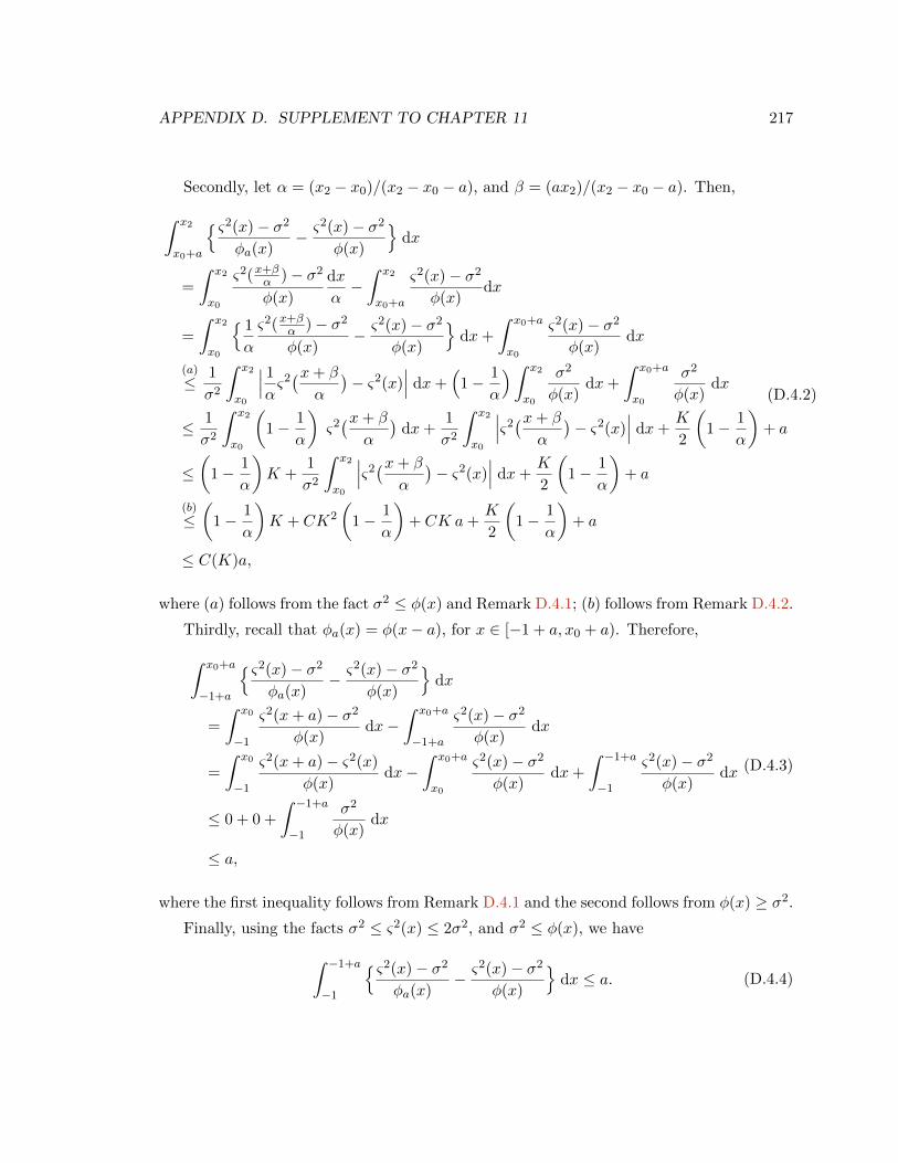
APPENDIX D. SUPPLEMENT TO CHAPTER 11 217
Secondly, let α = (x2 − x0)/(x2 − x0 − a), and β = (ax2)/(x2 − x0 − a). Then,∫ x2
x0+a
ς2(x)− σ2
φa(x)− ς2(x)− σ2
φ(x)
dx
=
∫ x2
x0
ς2(x+βα )− σ2
φ(x)
dx
α−∫ x2
x0+a
ς2(x)− σ2
φ(x)dx
=
∫ x2
x0
1
α
ς2(x+βα )− σ2
φ(x)− ς2(x)− σ2
φ(x)
dx+
∫ x0+a
x0
ς2(x)− σ2
φ(x)dx
(a)
≤ 1
σ2
∫ x2
x0
∣∣∣ 1ας2(x+ β
α
)− ς2(x)
∣∣∣ dx+(
1− 1
α
)∫ x2
x0
σ2
φ(x)dx+
∫ x0+a
x0
σ2
φ(x)dx
≤ 1
σ2
∫ x2
x0
(1− 1
α
)ς2(x+ β
α
)dx+
1
σ2
∫ x2
x0
∣∣∣ς2(x+ β
α
)− ς2(x)
∣∣∣ dx+K
2
(1− 1
α
)+ a
≤(
1− 1
α
)K +
1
σ2
∫ x2
x0
∣∣∣ς2(x+ β
α
)− ς2(x)
∣∣∣ dx+K
2
(1− 1
α
)+ a
(b)
≤(
1− 1
α
)K + CK2
(1− 1
α
)+ CK a+
K
2
(1− 1
α
)+ a
≤ C(K)a,
(D.4.2)
where (a) follows from the fact σ2 ≤ φ(x) and Remark D.4.1; (b) follows from Remark D.4.2.
Thirdly, recall that φa(x) = φ(x− a), for x ∈ [−1 + a, x0 + a). Therefore,∫ x0+a
−1+a
ς2(x)− σ2
φa(x)− ς2(x)− σ2
φ(x)
dx
=
∫ x0
−1
ς2(x+ a)− σ2
φ(x)dx−
∫ x0+a
−1+a
ς2(x)− σ2
φ(x)dx
=
∫ x0
−1
ς2(x+ a)− ς2(x)
φ(x)dx−
∫ x0+a
x0
ς2(x)− σ2
φ(x)dx+
∫ −1+a
−1
ς2(x)− σ2
φ(x)dx
≤ 0 + 0 +
∫ −1+a
−1
σ2
φ(x)dx
≤ a,
(D.4.3)
where the first inequality follows from Remark D.4.1 and the second follows from φ(x) ≥ σ2.
Finally, using the facts σ2 ≤ ς2(x) ≤ 2σ2, and σ2 ≤ φ(x), we have∫ −1+a
−1
ς2(x)− σ2
φa(x)− ς2(x)− σ2
φ(x)
dx ≤ a. (D.4.4)

APPENDIX D. SUPPLEMENT TO CHAPTER 11 218
Combining Eqs. (D.4.1), (D.4.2), (D.4.3), and (D.4.4) implies the desired result.
D.5 Proof of Proposition 11.4.13
Proof. Let EW(φa) = EW,1(φa) + EW,2(φa) + EW,3(φa), where
EW,1(φa) =
∫ `−1
x0+aI(W ∗ φa(y)−1)− I(φa(y − 1)−1)dy,
EW,2(φa) =
∫ x0+a
aI(W ∗ φa(y)−1)− I(φa(y − 1)−1)dy,
EW,3(φa) =
∫ a
0I(W ∗ φa(y)−1)− I(φa(y − 1)−1)dy.
(D.5.1)
Also let EW(φ) = EW,1(φ) + EW,2,3(φ), where
EW,1(φ) =
∫ `−1
x0+aI(W ∗ φ(y)−1)− I(φ(y − 1)−1)dy,
EW,2,3(φ) =
∫ x0+a
0I(W ∗ φ(y)−1)− I(φ(y − 1)−1)dy.
(D.5.2)
The following remark is used several times in the proof.
Remark D.5.1. For any two values 0 ≤ α1 < α2,
I(α2)− I(α1) =
∫ α2
α1
1
2mmse(z)dz ≤
∫ α2
α1
1
2zdz =
1
2log(α2
α1
)≤ 1
2
(α2
α1− 1
). (D.5.3)
• Bounding EW,1(φa)− EW,1(φ).
Notice that the functions φ(x) = φa(x), for x2 ≤ x. Also κ/2 < φa(x) ≤ φ(x) ≤ ΦM ,
for x1 < x < x2. Let α = (x2 − x1)/(x2 − x1 − a), and β = (ax2)/(x2 − x1 − a). Then,
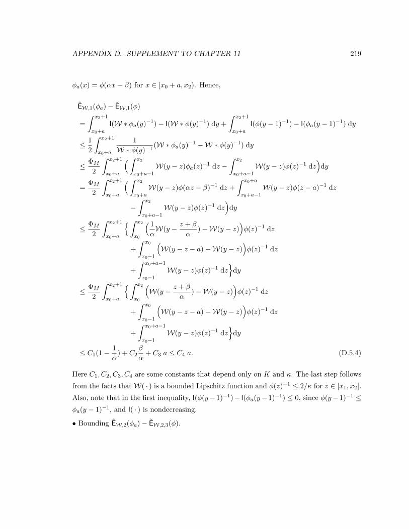
APPENDIX D. SUPPLEMENT TO CHAPTER 11 219
φa(x) = φ(αx− β) for x ∈ [x0 + a, x2). Hence,
EW,1(φa)− EW,1(φ)
=
∫ x2+1
x0+aI(W ∗ φa(y)−1)− I(W ∗ φ(y)−1) dy +
∫ x2+1
x0+aI(φ(y − 1)−1)− I(φa(y − 1)−1) dy
≤ 1
2
∫ x2+1
x0+a
1
W ∗ φ(y)−1(W ∗ φa(y)−1 −W ∗ φ(y)−1) dy
≤ ΦM
2
∫ x2+1
x0+a
(∫ x2
x0+a−1W(y − z)φa(z)−1 dz −
∫ x2
x0+a−1W(y − z)φ(z)−1 dz
)dy
=ΦM
2
∫ x2+1
x0+a
(∫ x2
x0+aW(y − z)φ(αz − β)−1 dz +
∫ x0+a
x0+a−1W(y − z)φ(z − a)−1 dz
−∫ x2
x0+a−1W(y − z)φ(z)−1 dz
)dy
≤ ΦM
2
∫ x2+1
x0+a
∫ x2
x0
( 1
αW(y − z + β
α)−W(y − z)
)φ(z)−1 dz
+
∫ x0
x0−1
(W(y − z − a)−W(y − z)
)φ(z)−1 dz
+
∫ x0+a−1
x0−1W(y − z)φ(z)−1 dz
dy
≤ ΦM
2
∫ x2+1
x0+a
∫ x2
x0
(W(y − z + β
α)−W(y − z)
)φ(z)−1 dz
+
∫ x0
x0−1
(W(y − z − a)−W(y − z)
)φ(z)−1 dz
+
∫ x0+a−1
x0−1W(y − z)φ(z)−1 dz
dy
≤ C1(1− 1
α) + C2
β
α+ C3 a ≤ C4 a. (D.5.4)
Here C1, C2, C3, C4 are some constants that depend only on K and κ. The last step follows
from the facts thatW( · ) is a bounded Lipschitz function and φ(z)−1 ≤ 2/κ for z ∈ [x1, x2].
Also, note that in the first inequality, I(φ(y− 1)−1)− I(φa(y− 1)−1) ≤ 0, since φ(y− 1)−1 ≤φa(y − 1)−1, and I( · ) is nondecreasing.
• Bounding EW,2(φa)− EW,2,3(φ).

APPENDIX D. SUPPLEMENT TO CHAPTER 11 220
We have
EW,2(φa) =
∫ x0+a
x0+a−1I(W ∗ φa(y)−1)− I(φa(y − 1)−1)dy
+
∫ x0+a−1
aI(W ∗ φa(y)−1)− I(φa(y − 1)−1)dy.
(D.5.5)
We treat each term separately. For the first term,∫ x0+a
x0+a−1I(W ∗ φa(y)−1)− I(φa(y − 1)−1)dy
=
∫ x0+a
x0+a−1
I
(∫ x0+a+1
x0+aW(y − z)φa(z)−1 dz +
∫ x0+a
x0+a−2W(y − z)φa(z)−1 dz
)− I(φa(y − 1)−1)
dy
=
∫ x0+a
x0+a−1I
(∫ x0+α
x0
W(y − z + β
α)φ(z)−1 dz
α+
∫ x0
x0−2W(y − a− z)φ(z)−1 dz
)dy
−∫ x0
x0−1I(φ(y − 1)−1)dy
=
∫ x0
x0−1I
(∫ x0+α
x0
W(y + a− z + β
α)φ(z)−1 dz
α+
∫ x0
x0−2W(y − z)φ(z)−1 dz
)dy
−∫ x0
x0−1I(φ(y − 1)−1)dy
≤ C5 a+
∫ x0
x0−1
I
(∫ x0+1
x0−2W(y − z)φ(z)−1 dz
)− I(φ(y − 1)−1)
dy
= C5 a+
∫ x0
x0−1
I(W ∗ φ(y)−1)− I(φ(y − 1)−1)
dy, (D.5.6)

APPENDIX D. SUPPLEMENT TO CHAPTER 11 221
where the last inequality is an application of remark D.5.1. More specifically,
I
(∫ x0+α
x0
W(y + a− z + β
α)φ(z)−1 dz
α+
∫ x0
x0−2W(y − z)φ(z)−1 dz
)− I
(∫ x0+1
x0−2W(y − z)φ(z)−1 dz
)≤ ΦM
2
(∫ x0+α
x0
W(y + a− z + β
α)φ(z)−1 dz
α−∫ x0+1
x0
W(y − z)φ(z)−1 dz
)≤ ΦM
2
∫ x0+α
x0+1W(y + a− z + β
α)φ(z)−1 dz
+ΦM
2
∫ x0+1
x0
(W(y + a− z + β
α)−W(y − z)
)φ(z)−1dz
≤ C ′1(1− 1
α) + C ′2
β
α+ C ′3 a ≤ C5 a,
where C ′1, C′2, C
′3, C5 are constants that depend only on κ. Here, the penultimate inequality
follows from α > 1, and the last one follows from the fact thatW( · ) is a bounded Lipschitz
function and that φ(z)−1 ≤ 2/κ, for z ∈ [x1, x2].
To bound the second term on the right hand side of Eq. (D.5.6), notice that φa(z) =
φ(z − a), for z ∈ [−1 + a, x0 + a), whereby∫ x0+a−1
aI(W ∗ φa(y)−1)− I(φa(y − 1)−1)dy
=
∫ x0−1
0I(W ∗ φ(y)−1)− I(φ(y − 1)−1)dy.
(D.5.7)
Now, using Eqs. (D.5.2), (D.5.5) and (D.5.7), we obtain
EW,2(φa)− EW,2,3(φ) ≤ C5 a−∫ x0+a
x0
I(W ∗ φ(y)−1)− I(φ(y − 1)−1)dy
≤ C5 a+
∫ x0+a
x0
log
(φ(y − 1)−1
W ∗ φ(y)−1
)≤ C5 a+ a log(
ΦM
κ) = C6 a,
(D.5.8)
where C6 is a constant that depends only on κ.
• Bounding EW,3(φa).
Notice that φa(y) ≥ σ2. Therefore, I(W ∗ φa(y)−1) ≤ I(σ−2), since I( · ) is nondecreasing.

APPENDIX D. SUPPLEMENT TO CHAPTER 11 222
Recall that φa(y) = φ∗ < 2σ2, for y ∈ [−1,−1 + a). Consequently,
EW,3(φa) ≤∫ a
0I(σ−2)− I(φ∗−1)dy ≤ a
2log(φ∗σ2
)<a
2log 2, (D.5.9)
where the first inequality follows from Remark D.5.1.
Finally, we are in position to prove the proposition. Using Eqs. (D.5.4), (D.5.8) and (D.5.9),
we get
EW(φa)− EW(φ) ≤ C4 a+ C6 a+a
2log 2 = C(κ,K) a. (D.5.10)
D.6 Proof of Proposition 11.4.14
We have∫ `−1
−1
V (φa(x))− V (φ(x))
dx =
∫ `−1
x2
V (φa(x))− V (φ(x))
dx
+(∫ x2
x0+aV (φa(x))dx−
∫ x2
x0
V (φ(x))dx)
+(∫ x0+a
−1+aV (φa(x))dx−
∫ x0
−1V (φ(x))dx
)+
∫ −1+a
−1V (φa(x))dx.
(D.6.1)
Notice that the first and the third terms on the right hand side are zero. Also,∫ x2
x0+aV (φa(x))dx−
∫ x2
x0
V (φ(x))dx = − a
x2 − x0
∫ x2
x0
V (φ(x))dx,∫ −1+a
−1V (φa(x))dx = aV (φ∗), ,
(D.6.2)
where the second equation holds because φa(x) = φ∗ for x ∈ [−1,−1 + a) in view of
Eq. (11.4.20).
Substituting Eq. (D.6.2) in Eq. (D.6.1), we get∫ `−1
−1
V (φa(x))− V (φ(x))
dx =
a
x2 − x0
∫ x2
x0
V (φ∗)− V (φ(x))
dx. (D.6.3)

APPENDIX D. SUPPLEMENT TO CHAPTER 11 223
Now we upper bound the right hand side of Eq. (D.6.3).
By Proposition 11.4.9, we have
V (φ∗) ≤ δ
2+δ − d(pX)
4log(2σ2), (D.6.4)
for σ ∈ (0, σ2]. Also, since φ(x) > κ/2 for x ∈ [x0, x2], we have V (φ(x)) ≥ (δ/2) log φ >
(δ/2) log(κ/2). Therefore,
1
2
∫ `−1
−1
V (φa(x))− V (φ(x))
dx =
a
2(x2 − x0)
∫ x2
x0
V (φ∗)− V (φ(x))
dx
<a
2
[δ2
+δ − d(pX)
4log(2σ2)− δ
2log(
κ
2)].
(D.6.5)
It is now obvious that by choosing σ0 > 0 small enough, we can ensure that for values
σ ∈ (0, σ0],
a
2
[δ2
+δ − d(pX)
4log(2σ2)− δ
2log(
κ
2)]< −2C(κ,K)a. (D.6.6)
(Notice that the right hand side of Eq. (D.6.6) does not depend on σ).
D.7 Proof of Claim 11.4.16
Similar to the proof of Claim 11.4.11, the assumption∫ `−1−1 |φ(x) − φ∗|dx > Cσ2` implies
φ(θ`− 1) > Cσ2(1− α), where
0 < θ =ΦM − Cσ2
ΦM − Cσ2(1− α)< 1.
Choose σ small enough such that φ∗ < φ1. Let κ = (φ1 − φ∗)(1 − θ)/2. Applying
Lemma 11.4.10, there exists `0, and σ0, such that,∫ `−1−1 |φ(x)− φ∗| dx ≤ κ`, for ` > `0 and
σ ∈ (0, σ0]. We claim that φ(µ`− 1) < φ1, with
µ = 1− κ
φ1 − φ∗=
1 + θ
2.

APPENDIX D. SUPPLEMENT TO CHAPTER 11 224
Otherwise, by monotonicity of φ(x),
(φ1 − φ∗)(1− µ)` ≤∫ `−1
µ`−1|φ(x)− φ∗| dx <
∫ `−1
−1|φ(x)− φ∗| dx ≤ κ`. (D.7.1)
Plugging in for µ yields a contradiction.
Therefore, Cσ2(1− α) < φ(x) < φ1, for x ∈ [θ`− 1, µ`− 1], and (µ− θ)` = (1− θ)`/2.
Choosing ` > max`0, 2K/(1− θ) gives the result.
D.8 Proof of Proposition 11.4.17
To prove Eq. (11.4.32), we write
∫ `−1
−1Vrob(φa(x))− Vrob(φ(x)) dx = −
∫ x2
x1
∫ φ(x)
φa(x)V ′(s) ds dx
≤ −∫ x2
x1
∫ φ(x)
φa(x)
δ
2s2
(s− σ2
)ds dx
= −δ2
∫ x2
x1
log
(φ(x)
φa(x)
)+
σ2
φ(x)− σ2
φa(x)
dx
≤ δ
2K log(1− a) +K
δa
2C(1− α)(1− a),
(D.8.1)
where the second inequality follows from the fact Cσ2/2 < φ(x), for x ∈ [x1, x2].
Next, we pass to prove Eq. (11.4.33).∫ `−1
−1(ς2(x)− σ2)
(1
φa(x)− 1
φ(x)
)dx =
∫ x2
x1
ς2(x)− σ2
φ(x)
(1
1− a− 1
)≤ a
1− a
∫ x2
x1
σ2
φ(x)dx ≤ K a
C(1− α)(1− a),
(D.8.2)
where the first inequality follows from Remark D.4.1.

APPENDIX D. SUPPLEMENT TO CHAPTER 11 225
Finally, we have
EW,rob(φa)− EW,rob(φ) =
∫ `
0I(W ∗ φa(y)−1)− I(W ∗ φ(y)−1)dy
=
∫ `
0
∫ W∗φa(y)−1
W∗φ(y)−1
1
2mmse(s) ds dy
≤ D(pX) + ε
2
∫ `
0
∫ W∗φa(y)−1
W∗φ(y)−1
s−1ds dy
≤ D(pX) + ε
2
∫ `
0log
(W ∗ φa(y)−1
W ∗ φ(y)−1
)dy
≤ −D(pX) + ε
2(K + 2) log(1− a),
(D.8.3)
where the first inequality follows from Eq. (11.4.29) and Claim 11.4.16.

Bibliography
[1] S. Aeron, V. Saligrama, and M. Zhao. Information theoretic bounds for compressed
sensing. IEEE Trans. on Inform. Theory, 56:5111 – 5130, 2010. 128
[2] M. Aizenman, R. Sims, and S. L. Starr. Extended variational principle for the
sherrington-kirkpatrick spin-glass model. Physical Review B, 68(21):214403, 2003.
70
[3] K. Do Ba, P. Indyk, E. Price, and D. P. Woodruff. Lower bounds for sparse recov-
ery. In Proceedings of the Twenty-First Annual ACM-SIAM Symposium on Discrete
Algorithms, SODA ’10, pages 1190–1197, 2010. 129
[4] D. Baron, S. Sarvotham, and R. Baraniuk. Bayesian Compressive Sensing Via Belief
Propagation. IEEE Trans. on Signal Proc., 58:269–280, 2019. 127, 131
[5] M. Bayati, M. A. Erdogdu, and A. Montanari. Estimating Lasso risk and noise level.
In Advances in Neural Information Processing Systems, pages 944–952, 2013. 40
[6] M. Bayati, M. Lelarge, and A. Montanari. Universality in message passing algorithms.
arXiv:1207.7321, 2012. 69, 70, 122, 182
[7] M. Bayati and A. Montanari. The dynamics of message passing on dense graphs,
with applications to compressed sensing. IEEE Trans. on Inform. Theory, 57:764–
785, 2011. 24, 122, 136, 148, 154, 156, 182, 186
[8] M. Bayati and A. Montanari. The LASSO risk for gaussian matrices. IEEE Trans.
on Inform. Theory, 58:1997–2017, 2012. 44, 61, 65, 69, 70, 72, 85, 86, 120, 147, 192,
193
226

BIBLIOGRAPHY 227
[9] A. Beck and M. Teboulle. A fast iterative shrinkage-thresholding algorithm for linear
inverse problems. SIAM J. Img. Sci., 2(1):183–202, 2009. 15
[10] R. Bellman. Adaptive Control Processes: A Guided Tour. Princeton University Press,
1961. 4
[11] A. Belloni and V. Chernozhukov. Least squares after model selection in high-
dimensional sparse models. Bernoulli, 19(2):521–547, 2013. 40
[12] R. Berinde, A. C. Gilbert, P. Indyk, H. Karloff, and M. J. Strauss. Combining
geometry and combinatorics: A unified approach to sparse signal recovery. In 47th
Annual Allerton Conference, pages 798 – 805, Monticello, IL, September 2008. 128
[13] P. J. Bickel and E. Levina. Regularized estimation of large covariance matrices. The
Annals of Statistics, pages 199–227, 2008. 71
[14] P. J. Bickel, Y. Ritov, and A. B. Tsybakov. Simultaneous analysis of Lasso and
Dantzig selector. The Annals of Statistics, 37:1705–1732, 2009. 9, 34, 60, 99
[15] S. Boyd, N. Parikh, E. Chu, B. Peleato, and J. Eckstein. Distributed optimization
and statistical learning via the alternating direction method of multipliers. Found.
Trends Mach. Learn., 3(1):1–122, 2011. 15
[16] P. Buhlmann. Statistical significance in high-dimensional linear models. Bernoulli,
19(4):1212–1242, 2013. xiii, xiv, xvi, 17, 58, 59, 81, 84, 85, 86, 87, 88, 89, 90, 91, 92,
93, 94, 95, 97
[17] P. Buhlmann, M. Kalisch, and L. Meier. High-dimensional statistics with a view
toward applications in biology. Annual Review of Statistics and Its Application,
1(1):255–278, 2014. 82, 84
[18] P. Buhlmann and J. Mandozzi. High-dimensional variable screening and bias in subse-
quent inference, with an empirical comparison. Computational Statistics, 29:407–430,
2014. 56
[19] P. Buhlmann and S. van de Geer. Statistics for high-dimensional data. Springer-
Verlag, 2011. 28, 33, 38, 98
BIBLIOGRAPHY 228
[20] T. Cai, W. Liu, and X. Luo. A constrained `1 minimization approach to sparse preci-
sion matrix estimation. Journal of the American Statistical Association, 106(494):594–
607, 2011. 71
[21] A. T. Campo, A. Guillen i Fabregas, and E. Biglieri. Large-system analysis of mul-
tiuser detection with an unknown number of users: A high-snr approach. Information
Theory, IEEE Transactions on, 57(6):3416–3428, 2011. 70
[22] E. Candes and M. Davenport. How well can we estimate a sparse vector?
arXiv:1104.5246v3, 2011. 128
[23] E. Candes, J. K. Romberg, and T. Tao. Robust uncertainty principles: Exact signal
reconstruction from highly incomplete frequency information. IEEE Trans. on Inform.
Theory, 52:489 – 509, 2006. 20, 177, 178, 185
[24] E. Candes, J. K. Romberg, and T. Tao. Stable signal recovery from incomplete
and inaccurate measurements. Communications on Pure and Applied Mathematics,
59:1207–1223, 2006. 20
[25] E. Candes and T. Tao. The Dantzig selector: statistical estimation when p is much
larger than n. The Annals of Statistics, 35:2313–2351, 2007. 9, 60
[26] E. J. Candes and Y. Plan. Tight oracle inequalities for low-rank matrix recovery from
a minimal number of noisy random measurements. IEEE Transactions on Information
Theory, 57(4):2342–2359, 2011. 8
[27] E. J. Candes and B. Recht. Exact matrix completion via convex optimization. Found.
Comput. Math., 9(6):717–772, 2009. 8
[28] E. J. Candes and T. Tao. Decoding by linear programming. IEEE Trans. on Inform.
Theory, 51:4203–4215, 2005. 20
[29] O. Chapelle, B. Scholkopf, A. Zien, et al. Semi-supervised learning. MIT Press,
Cambridge, 2006. 71
[30] S. S. Chen and D. L. Donoho. Examples of basis pursuit. In Proceedings of Wavelet
Applications in Signal and Image Processing III, San Diego, CA, 1995. 6, 20

BIBLIOGRAPHY 229
[31] S. S. Chen, D. L. Donoho, and M. A. Saunders. Atomic decomposition by basis
pursuit. SIAM Journal on Scientific Computing, 20(1):33–61, 1998. 20
[32] L. H. Dicker. Residual variance and the signal-to-noise ratio in high-dimensional linear
models. arXiv preprint arXiv:1209.0012, 2012. 40
[33] D. Donoho, I. Johnstone, and A. Montanari. Accurate Prediction of Phase Transitions
in Compressed Sensing via a Connection to Minimax Denoising. arXiv:1111.1041, 2011.
122, 130, 131
[34] D. Donoho and J. Tanner. Observed universality of phase transitions in high-
dimensional geometry, with implications for modern data analysis and signal pro-
cessing. Philosophical Transactions of the Royal Society A: Mathematical, Physical
and Engineering Sciences, 367(1906):4273–4293, 2009. 23, 24
[35] D. L. Donoho. Aide-memoire. high-dimensional data analysis: The curses and bless-
ings of dimensionality, 2000. 5
[36] D. L. Donoho. Compressed sensing. IEEE Trans. on Inform. Theory, 52:489–509,
April 2006. 20, 128
[37] D. L. Donoho. High-dimensional centrally symmetric polytopes with neighborliness
proportional to dimension. Discrete Comput. Geometry, 35:617–652, 2006. 20, 61,
128
[38] D. L. Donoho and M. Elad. Maximal sparsity representation via l1 minimization.
Proceedings of the National Academy of Sciences, 100:2197–2202, March 2003. 20
[39] D. L. Donoho and X. Huo. Uncertainty principles and ideal atomic decomposition.
IEEE Transactions on Information Theory, 47(7):2845–2862, 2001. 32
[40] D. L. Donoho, A. Javanmard, and A. Montanari. Information-theoretically optimal
compressed sensing via spatial coupling and approximate message passing. In IEEE
International Symposium on Information Theory (ISIT), pages 1231–1235, 2012. 25
[41] D. L. Donoho, A. Javanmard, and A. Montanari. Information-theoretically optimal
compressed sensing via spatial coupling and approximate message passing. IEEE
Transactions on Information Theory, 59(11):7434–7464, 2013. 25, 176, 178
BIBLIOGRAPHY 230
[42] D. L. Donoho, A. Maleki, and A. Montanari. Message Passing Algorithms for Com-
pressed Sensing. Proceedings of the National Academy of Sciences, 106:18914–18919,
2009. 22, 24, 85, 86, 115, 121, 122, 130, 131, 132, 136, 138, 147, 153, 184
[43] D. L. Donoho, A. Maleki, and A. Montanari. Message Passing Algorithms for Com-
pressed Sensing: I. Motivation and Construction. In Proceedings of IEEE Inform.
Theory Workshop, Cairo, 2010. 22, 122, 131, 132
[44] D. L. Donoho, A. Maleki, and A. Montanari. The Noise Sensitivity Phase Transition
in Compressed Sensing. IEEE Trans. on Inform. Theory, 57:6920–6941, 2011. xiv,
20, 64, 86, 130, 131, 193
[45] D. L. Donoho and J. Tanner. Neighborliness of randomly-projected simplices in high
dimensions. Proceedings of the National Academy of Sciences, 102(27):9452–9457,
2005. 61, 128
[46] D. L. Donoho and J. Tanner. Counting faces of randomly projected polytopes when
the projection radically lowers dimension. Journal of American Mathematical Society,
22:1–53, 2009. 61
[47] D. L. Donoho and J. Tanner. Counting the faces of randomly-projected hypercubes
and orthants, with applications. Discrete & Computational Geometry, 43(3):522–541,
2010. 130
[48] D. L. Donoho and J. Tanner. Precise undersampling theorems. Proceedings of the
IEEE, 98:913–924, 2010. 61
[49] J. Fan, S. Guo, and N. Hao. Variance estimation using refitted cross-validation in
ultrahigh dimensional regression. Journal of the Royal Statistical Society: Series B
(Statistical Methodology), 74(1):37–65, 2012. 40
[50] J. Fan and R. Li. Variable selection via nonconcave penalized likelihood and its oracle
properties. Journal of the American Statistical Association, 96(456):1348–1360, 2001.
40
[51] J. Fan and J. Lv. Sure independence screening for ultrahigh dimensional feature
space. Journal of the Royal Statistical Society: Series B (Statistical Methodology),
70(5):849–911, 2008. 40

BIBLIOGRAPHY 231
[52] J. Fan, R. Samworth, and Y. Wu. Ultrahigh dimensional feature selection: beyond
the linear model. The Journal of Machine Learning Research, 10:2013–2038, 2009. 40
[53] A. J. Felstrom and K. S. Zigangirov. Time-varying periodic convolutional codes with
low-density parity-check matrix. IEEE Trans. on Inform. Theory, 45:2181–2190, 1999.
131, 144
[54] S. Foucart. Sparse recovery algorithms: Sufficient conditions in terms of restricted
isometry constants. In M. Neamtu and L. Schumaker, editors, Approximation Theory
XIII: San Antonio 2010, volume 13 of Springer Proceedings in Mathematics, pages
65–77. Springer New York, 2012. 20
[55] A. Frank and A. Asuncion. UCI machine learning repository (communities and crime
data set). http://archive.ics.uci.edu/ml, 2010. University of California, Irvine, School
of Information and Computer Sciences. 92, 95
[56] J. Friedman, T. Hastie, and R. Tibshirani. Regularization paths for generalized linear
models via coordinate descent. Journal of Statistical Software, 33(1):1–22, 2010. 82
[57] R. G. Gallager. Low-Density Parity-Check Codes. MIT Press, Cambridge, Massachus-
setts, 1963. Available online at http://web./gallager/www/pages/ldpc.pdf. 146
[58] E. Greenshtein and Y. Ritov. Persistence in high-dimensional predictor selection and
the virtue of over-parametrization. Bernoulli, 10:971–988, 2004. 9
[59] D. Gross. Recovering low-rank matrices from few coefficients in any basis. IEEE
Trans. Inf. Theory, 57(3):1548–1566, 2011. 8
[60] F. Guerra. Broken replica symmetry bounds in the mean field spin glass model.
Communications in mathematical physics, 233(1):1–12, 2003. 70
[61] D. Guo, D. Baron, and S. Shamai. A Single-letter Characterization of Optimal Noisy
Compressed Sensing. In 47th Annual Allerton Conference, Monticello, IL, September
2009. 70
[62] D. Guo, S. Shamai, and S. Verdu. Mutual information and minimum mean-square
error in gaussian channels. IEEE Trans. Inform. Theory, 51:1261–1282, 2005. 165

BIBLIOGRAPHY 232
[63] D. Guo and S. Verdu. Randomly Spread CDMA: Asymptotics via Statistical Physics.
IEEE Trans. on Inform. Theory, 51:1982–2010, 2005. 70, 194
[64] S. H. Hassani, N. Macris, and R. Urbanke. Coupled graphical models and their
thresholds. In Proceedings of IEEE Inform. Theory Workshop, Dublin, 2010. 132,
134, 144, 147
[65] A. E. Hoerl and R. W. Kennard. Ridge regression: biased estimation for nonorthog-
onal problems. Technometrics, 12(1):55–67, 1970. 6
[66] P. J. Huber and E. Ronchetti. Robust Statistics (second edition). J. Wiley and Sons,
2009. 65, 139
[67] I. Ibragimov and R. Z. Khasminskii. Statistical estimation: asymptotic theory.
Springer, 1981. 4
[68] P. Indyk, E. Price, and D. P. Woodruff. On the Power of Adaptivity in Sparse
Recovery. In IEEE Symposium on the Foundations of Computer Science, FOCS,
October 2011. 132
[69] L. Jacob, G. Obozinski, and J.-P. Vert. Group lasso with overlap and graph lasso. In
Proceedings of the 26th Annual International Conference on Machine Learning, ICML
’09, pages 433–440, New York, NY, USA, 2009. ACM. 7, 8
[70] A. Javanmard and A. Montanari. Subsampling at information theoretically optimal
rates. In IEEE International Symposium on Information Theory (ISIT), pages 2431–
2435, 2012. 25, 144, 147
[71] A. Javanmard and A. Montanari. Confidence intervals and hypothesis testing for
high-dimensional statistical models. In Advances in Neural Information Processing
Systems, pages 1187–1195. Curran Associates, Inc., 2013. 17
[72] A. Javanmard and A. Montanari. Hypothesis testing in high-dimensional regres-
sion under the gaussian random design model: Asymptotic theory. arXiv preprint
arXiv:1301.4240, (To appear in IEEE Transaction on Information Theory), 2013. 18,
37, 38

BIBLIOGRAPHY 233
[73] A. Javanmard and A. Montanari. Model selection for high-dimensional regression
under the generalized irrepresentability condition. In Advances in Neural Information
Processing Systems, pages 3012–3020. Curran Associates, Inc., 2013. 10
[74] A. Javanmard and A. Montanari. State Evolution for General Approximate Message
Passing Algorithms, with Applications to Spatial Coupling. Journal of Information
and Inference, 2(2):115–144, 2013. 25, 122, 134, 148, 154, 156, 182
[75] A. Javanmard and A. Montanari. Confidence Intervals and Hypothesis Testing for
High-Dimensional Regression. arXiv preprint arXiv:1306.3171, (To appear in Journal
of Machine Learning Research), 2014. 17
[76] Y. Kabashima, M. Vehkapera, and S. Chatterjee. Typical l1-recovery limit of sparse
vectors represented by concatenations of random orthogonal matrices. J. Stat. Mech.,
page P12003, 2012. 70
[77] Y. Kabashima, T. Wadayama, and T. Tanaka. A typical reconstruction limit for
compressed sensing based on Lp-norm minimization. J.Stat. Mech., page L09003,
2009. 70
[78] U. S. Kamilov, V. K. Goyal, and S. Rangan. Message-Passing Estimation from Quan-
tized Samples. arXiv:1105.6368, 2011. 131
[79] B. S. Kashin and V. N. Temlyakov. A remark on compressed sensing. Mathematical
Notes, 82:748–755, 2007. 128
[80] Y. Kim, J. Kim, and Y. Kim. Blockwise Sparse Regression. Stat. Sinica, 16:375–390,
2006. 7
[81] K. Knight and W. Fu. Asymptotics for lasso-type estimators. The Annals of Statistics,
pages 1356–1378, 2000. 9
[82] F. Krzakala, M. Mezard, F. Sausset, Y. Sun, and L. Zdeborova. Statistical physics-
based reconstruction in compressed sensing. arXiv:1109.4424, 2011. 21, 22, 127, 130,
132, 144, 147, 166, 176, 178, 186, 187
[83] S. Kudekar, C. Measson, T. Richardson, and R. Urbanke. Threshold Saturation on
BMS Channels via Spatial Coupling. In Proceedings of the International Symposium
on Turbo Codes and Iterative Information Processing, Brest, 2010. 132, 134, 144

BIBLIOGRAPHY 234
[84] S. Kudekar and H. D. Pfister. The effect of spatial coupling on compressive sensing.
In 48th Annual Allerton Conference, pages 347 –353, 2010. 21, 132
[85] S. Kudekar, T. Richardson, and R. Urbanke. Threshold Saturation via Spatial Cou-
pling: Why Convolutional LDPC Ensembles Perform So Well over the BEC. IEEE
Trans. on Inform. Theory, 57:803–834, 2011. 21, 131, 145
[86] S. Kudekar, T. Richardson, and R. Urbanke. Spatially coupled ensembles universally
achieve capacity under belief propagation. In Information Theory Proceedings (ISIT),
2012 IEEE International Symposium on, pages 453–457. IEEE, 2012. 132, 134, 144
[87] L. Le Cam. On the asymptotic theory of estimation and testing hypotheses. In Pro-
ceedings of the Third Berkeley Symposium on Mathematical Statistics and Probability,
volume 1, pages 129–156. University of California Press Berkeley, CA, 1956. 44
[88] E. Lehmann and G. Casella. Theory of point estimation. Springer, 2 edition, 1998.
45
[89] E. L. Lehmann and J. P. Romano. Testing statistical hypotheses. Springer, 2005. 48,
112
[90] M. Lentmaier and G. P. Fettweis. On the thresholds of generalized LDPC convolu-
tional codes based on protographs. In IEEE Intl. Symp. on Inform. Theory, Austin,
Texas, August 2010. 131
[91] A. Maleki, L. Anitori, A. Yang, and R. Baraniuk. Asymptotic Analysis of Complex
LASSO via Complex Approximate Message Passing (CAMP). arXiv:1108.0477, 2011.
187
[92] S. G. Mallat and Z. Zhang. Matching pursuits with time-frequency dictionaries. IEEE
Transactions on Signal Processing, 41(12):3397–3415, 1993. 32
[93] E. Matusiak and Y. C. Eldar. Sub-nyquist sampling of short pulses. In IEEE In-
ternational Conference on Acoustics, Speech, and Signal Processing (ICASSP), pages
3944–3947, 2011. 179
[94] C. Measson, A. Montanari, T. Richardson, and R. Urbanke. The Generalized
Area Theorem and Some of its Consequences. IEEE Trans. on Inform. Theory,
55(11):4793–4821, 2009. 146
BIBLIOGRAPHY 235
[95] N. Meinshausen and P. Buhlmann. High-dimensional graphs and variable selection
with the Lasso. The Annals of Statistics, 34:1436–1462, 2006. 9, 10, 61, 71
[96] N. Meinshausen, L. Meier, and P. Buhlmann. p-values for high-dimensional regression.
Journal of the American Statistical Association, 104(488):1671–1681, 2009. 17, 57,
81, 84
[97] M. Mezard and A. Montanari. Information, Physics and Computation. Oxford, 2009.
194, 199
[98] M. Mezard, G. Parisi, and M. A. Virasoro. Spin Glass Theory and Beyond. World
Scientific, 1987. 194, 199
[99] A. Montanari. Graphical Models Concepts in Compressed Sensing. In Y.C. Eldar
and G. Kutyniok, editors, Compressed Sensing: Theory and Applications. Cambridge
University Press, 2012. 121, 122, 138
[100] A. Montanari and D. Tse. Analysis of belief propagation for non-linear problems:
the example of CDMA (or: how to prove Tanaka’s formula). In Proceedings of IEEE
Inform. Theory Workshop, Punta de l’Este, Uruguay, 2006. 70
[101] S. Negahban and M. J. Wainwright. Estimation of (near) low-rank matrices with
noise and high-dimensional scaling. Annals of Statistics, 39(2):1069–1097, 2011. 8
[102] S. N. Negahban and M. J. Wainwright. Simultaneous support recovery in high di-
mensions: Benefits and perils of block `1/`∞-regularization. IEEE Trans. Inf. Theor.,
57(6):3841–3863, 2011. 7
[103] Y. E. Nesterov. A method for solving the convex programming problem with con-
vergence rate O(1/k2). Dokl. Akad. Nauk SSSR, 269:543?547 (in Russian), 1983.
15
[104] Y. E. Nesterov. Gradient methods for minimizing composite objective function.
http://www.ecore.be/DPs/dp-1191313936.pdf, 2007. CORE report. 15
[105] G. Obozinski, M. J. Wainwright, and M. I. Jordan. Union support recovery in high-
dimensional multivariate regression. Annals of Statistics, 39(1):1–47, 2011. 7
BIBLIOGRAPHY 236
[106] S. Oymak, C. Thrampoulidis, and B. Hassibi. The squared-error of generalized lasso:
A precise analysis. arXiv:1311.0830, 2013. 69, 70
[107] D. Panchenko. The Sherrington-Kirkpatrick model. Springer, 2013. 70
[108] S. Rangan. Generalized Approximate Message Passing for Estimation with Random
Linear Mixing. In IEEE Intl. Symp. on Inform. Theory, St. Perersbourg, August
2011. 131, 136
[109] S. Rangan, A. K. Fletcher, and V. K. Goyal. Asymptotic Analysis of MAP Estimation
via the Replica Method and Applications to Compressed Sensing. In NIPS, Vancouver,
2009. 70
[110] G. Raskutti, M. J. Wainwright, and B. Yu. Minimax rates of estimation for high-
dimensional linear regression over `q-balls. In 47th Annual Allerton Conf., Monticello,
IL, September 2009. 9, 128
[111] B. Recht, M. Fazel, and P. A. Parrilo. Guaranteed minimum-rank solutions of linear
matrix equations via nuclear norm minimization. SIAM Rev., 52(3):471–501, 2010. 8
[112] S. Reid, R. Tibshirani, and J. Friedman. A study of error variance estimation in Lasso
regression. arXiv preprint arXiv:1311.5274, 2013. 40
[113] Z. Ren, T. Sun, C.-H Zhang, and H. Zhou. Asymptotic Normality and Optimalities
in Estimation of Large Gaussian Graphical Model. arXiv:1309.6024, 2013. 61, 71
[114] A. Renyi. On the dimension and entropy of probability distributions. Acta Mathe-
matica Hungarica, 10:193–215, 1959. 123, 124
[115] T. J. Richardson and R. Urbanke. Modern Coding Theory. Cambridge University
Press, Cambridge, 2008. 135, 178
[116] M. Rudelson and Z. Shuheng. Reconstruction from anisotropic random measurements.
IEEE Transactions on Information Theory, 59(6):3434–3447, 2013. 34, 99
[117] P. Schniter. Turbo Reconstruction of Structured Sparse Signals. In Proceedings of the
Conference on Information Sciences and Systems, Princeton, 2010. 131
[118] P. Schniter. A message-passing receiver for BICM-OFDM over unknown clustered-
sparse channels. arXiv:1101.4724, 2011. 131

BIBLIOGRAPHY 237
[119] P. J. Schreier and L. L. Scharf. Statistical signal processing of complex-valued data : the
theory of improper and noncircular signals. Cambridge University Press, Cambridge,
2010. 181
[120] S. Som, L. C. Potter, and P. Schniter. Compressive Imaging using Approximate
Message Passing and a Markov-Tree Prior. In Proc. Asilomar Conf. on Signals,
Systems, and Computers, November 2010. 131
[121] A. Sridharan, M. Lentmaier, D. J. Costello Jr, and K. S. Zigangirov. Convergence
analysis of a class of LDPC convolutional codes for the erasure channel. In 43rd
Annual Allerton Conference, Monticello, IL, September 2004. 131, 144
[122] N. Stadler, P. Buhlmann, and S. van de Geer. `1-penalization for mixture regression
models (with discussion). Test, 19(2):209–256, 2010. 40
[123] M. Stojnic, F. Parvaresh, and B. Hassibi. On the reconstruction of block-sparse signals
with an optimal number of measurements. IEEE Transactions on Signal Processing,
57(8):3075–3085, 2009. 7
[124] T. Sun and C.-H. Zhang. Scaled sparse linear regression. Biometrika, 99(4):879–898,
2012. 40, 41, 65, 189
[125] K. Takeda and Y. Kabashima. Statistical mechanical analysis of compressed sensing
utilizing correlated compression matrix. In IEEE Intl. Symp. on Inform. Theory, june
2010. 70, 194
[126] M. Talagrand. Mean Field Models for Spin Glasses: Volume I. Springer-Verlag,
Berlin, 2010. 70
[127] T. Tanaka. A Statistical-Mechanics Approach to Large-System Analysis of CDMA
Multiuser Detectors. IEEE Trans. on Inform. Theory, 48:2888–2910, 2002. 70, 194
[128] T. Tanaka and M. Okada. Approximate belief propagation, density evolution, and
statistical neurodynamics for cdma multiuser detection. Information Theory, IEEE
Transactions on, 51(2):700–706, 2005. 70
[129] R. Tibshirani. Regression shrinkage and selection with the Lasso. J. Royal. Statist.
Soc B, 58:267–288, 1996. 6

BIBLIOGRAPHY 238
[130] A. N. Tikhonov. On the stability of inverse problems. Doklady Akademii nauk SSSR,
39(5):195–198, 1943. 5
[131] A. Tulino, G. Caire, S. Shamai, and S. Verdu. Support recovery with sparsely sam-
pled free random matrices. In Information Theory Proceedings (ISIT), 2011 IEEE
International Symposium on, pages 2328–2332. IEEE, 2011. 70
[132] B. A. Turlach, W. N. Venables, and S. J. Wright. Simultaneous variable selection.
Technometrics, 47(3):349–363, 2005. 7
[133] S. van de Geer and P. Buhlmann. On the conditions used to prove oracle results for
the Lasso. Electron. J. Statist., 3:1360–1392, 2009. 9, 10, 33, 34, 86
[134] S. van de Geer, P. Buhlmann, Y. Ritov, and R. Dezeure. On asymptotically op-
timal confidence regions and tests for high-dimensional models. arXiv preprint
arXiv:1303.0518, (To appear in Annals of Statistics), 2014. 33, 37, 38, 39, 45, 56,
72, 73
[135] A. W. Van der Vaart. Asymptotic statistics, volume 3. Cambridge university press,
2000. 15, 44
[136] R. Vershynin. Introduction to the non-asymptotic analysis of random matrices. In
Y.C. Eldar and G. Kutyniok, editors, Compressed sensing: Theory and Applications,
pages 210–268. Cambridge University Press, 2012. 100, 101, 102
[137] J. Vila and P. Schniter. Expectation-maximization bernoulli-gaussian approximate
message passing. In Proc. Asilomar Conf. on Signals, Systems, and Computers, Pacific
Grove, CA, 2011. 130
[138] C. Villani. Optimal transport: old and new, volume 338. Springer, 2008. 120
[139] M. J. Wainwright. Information-theoretic limits on sparsity recovery in the high-
dimensional and noisy setting. IEEE Trans. on Inform. Theory, 55:5728–5741, 2009.
128
[140] M. J. Wainwright. Sharp thresholds for high-dimensional and noisy sparsity recov-
ery using `1-constrained quadratic programming. IEEE Trans. on Inform. Theory,
55:2183–2202, 2009. 9, 10

BIBLIOGRAPHY 239
[141] L. Wasserman. All of statistics: a concise course in statistical inference. Springer
Verlag, 2004. 27
[142] L. Wasserman and K. Roeder. High dimensional variable selection. The Annals of
statistics, 37(5A):2178, 2009. 17, 56
[143] Y. Wu and S. Verdu. Renyi Information Dimension: Fundamental Limits of Almost
Lossless Analog Compression. IEEE Trans. on Inform. Theory, 56:3721–3748, 2010.
21, 22, 123, 124, 128, 146, 182
[144] Y. Wu and S. Verdu. MMSE dimension. IEEE Trans. on Inform. Theory, 57(8):4857–
4879, 2011. 123, 124, 125, 165
[145] Y. Wu and S. Verdu. Optimal phase transitions in compressed sensing. Information
Theory, IEEE Transactions on, 58(10):6241, 2012. 70
[146] Z. Yang, C. Zhang, and L. Xie. On phase transition of compressed sensing in the
complex domain. IEEE Signal Processing Letters, 19:47–50, 2012. 187
[147] M. Yuan and Y. Lin. Model selection and estimation in regression with grouped
variables. Journal of the Royal Statistical Society B, 68:49–67, 2010. 7
[148] C-H. Zhang. Nearly unbiased variable selection under minimax concave penalty. The
Annals of Statistics, 38(2):894–942, 2010. 40
[149] C.-H. Zhang and S. S. Zhang. Confidence intervals for low-dimensional parameters
in high-dimensional linear models. Journal of the Royal Statistical Society: Series B
(Statistical Methodology), 76:217–242, 2014. xiii, xiv, xvi, 17, 38, 39, 58, 59, 72, 73,
85, 86, 87, 88, 89, 90, 92, 93, 94
[150] P. Zhao and B. Yu. On model selection consistency of Lasso. The Journal of Machine
Learning Research, 7:2541–2563, 2006. 9, 10
Recommended


![Multidimensional Sinusoidal Frequency Estimation …leihuang-hit.net/Publications_files/Journal/[TSP]Multidimensional... · ... H. L. Van Trees, Detection, Estimation, and Modulation](https://img.pdfslide.us/doc/110x75/5b5e123d7f8b9a8b4a8b9573/multidimensional-sinusoidal-frequency-estimation-leihuang-hitnetpublicationsfilesjournaltspmultidimensional.jpg)