In Search of New Geometriesfor Probing Spin-Spin
Interactions
Daniel G. Ang
Advisor: Professor Larry R. HunterDecember 8, 2015
Submitted to theDepartment of Physics and Astronomy
of Amherst Collegein partial fulfilment of the
requirements for the degree ofBachelors of Arts with honors
c© 2015 Daniel G. Ang
Abstract
Finding evidence for new long range spin-spin interactions (LRSSIs) would
mean the discovery of exciting new physics. In two of our recent papers [1, 2]
we have demonstrated a new geophysical method to probe for LRSSIs using our
dual Cs-Hg co-magnetometer experiment at Amherst College. In this thesis,
we present the results of efforts to explore new optical geometries to upgrade
the previous generation of the apparatus, the key improvement of which is
having the pumping and probing lasers be orthogonal to the magnetic field.
We explore two different schemes of running the experiment: the pump-then-
probe (PTP) scheme and the continuous pumping and probing (CPP) scheme,
using only Cs atomic vapor cells. We determine that both schemes have a
statistical noise level roughly an order of magnitude below our sensitivity goal
of ∆vCsN < 32 µHz.We present results of investigations of systematic effects
that arise from shifts in the intensity and frequency of the pump and probe
lasers. We find that as expected, PTP has smaller systematic uncertainties
and at this point is the more likely scheme to be used in the future.
i
Acknowledgments
I would first like to extend my greatest thanks to Professor Larry Hunter,
who has been my scientific mentor and role model for my four years here at
Amherst College. The story of my physics career began with me failing to test
out of Physics 123, and as a result having to take it with Professor Hunter.
The rest, as they say, is history. Thank you for taking me into the lab during
my freshman summer and giving me projects that allowed me to eventually
publish two papers with you as an undergraduate, a privilege and honor that
I’ll never be able to repay back. Thank you for recommending me for the
Schupf scholarship. Thank you for showing and teaching me that it’s perfectly
fine to admit when we do not know or understand something, for showing
me the beauty of simple physical models and symmetry arguments, and for
giving me excellent training in precision measurement and physics in general.
Without what you did for me in the last four years, I would never have had
the chance to embark on a career as a physicist.
Next, I would like to thank Dr. Stephen Peck, who has ever been so gener-
ous in answering my questions and providing detailed technical guidance to me
ever since the summer of 2012. Thank you for explaining to me more than five
ii
times (in my memory) of how the LLI experiment works, as well as a host of
countless other things. Thank you for putting up with my questions, including
the silly and stupid ones, and for tolerating my mistakes, transgressions, and
carelessness. Thank you for teaching me so much about various techniques
used in optics, electronics, and atomic physics. Thanks also for supporting
and taking an interest in my musical activities.
I would also like to thank the rest of my physics professors here at Amherst
College that have greatly influenced me and molded me over the past 4 years
into a budding physicist. In particular, I would like to thank Professor David
Hall for being a great academic advisor. Thank you for the valuable conversa-
tions we had about physics, graduate school, and the liberal arts, and thank
you for your recommendations, and for also being an inspiration in general.
Thank you for that speech in Senior Assembly 2012, which encouraged me to
dare to pursue my dreams of becoming a physicist. Thank you also Professors
Joel Gordon, David Hanneke, Ashley Carter, William Loinaz, Kannan Jagan-
nathan, and others who have taught me about physics and given me great
advice about physics and graduate school.
To Shah Saad Alam, Phyo Aung Kyaw, and other senior students who have
been my TAs: thank you for your teaching, guidance, and being role models
in general. To Horia Gheorghe: thank you for three years of friendship and
walking with me in our journey to grow as physicists. I hope we forever remain
lifelong friends and colleagues at Harvard and beyond. And also to the fellow
physics majors in my class: thank you for spending afternoons and evenings
together doing and discussing physics. Without all of these students, I would
iii
never have succeeded as a physics major.
I would like to acknowledge Jim Kubasek, for training me in machining and
giving me advice on designing and making things; Norman Page, for assisting
me in electronics; Ellen Feld and others for their great work in the Department.
I am grateful for the generous financial support from the Amherst College
Dean of the Faculty, National Science Foundation (grants PHY-0855465 and
PHY-1205824), and most of all the Schupf Scholarship fund, which has been
instrumental in allowing me to succeed in various other endeavors, both scien-
tific and musical. I would like to thank my thesis reading committee for taking
the time to read, assess, and question me on this document I have written.
I would also like to thank my other friends at Amherst College who have
taken an interest in my research and helped me become a better speaker about
physics, and friends at the First Baptist Church of Amherst, in particular
Stephen Broyles, Evie Hopkins, Dixie Brown, and Ron Loescher, for support-
ing me throughout my four years here and providing a wonderful environment
for me to keep growing in Christ. Last but not least, I would like to thank the
support, patience, and love of my parents, Gideon and Yohana Ang, and also
my dear beloved brother, Joseph Ang. Without them I would simply not be
here.
iv

Soli Deo gloria
v
Contents
1 Theoretical Motivations 11.1 Matter, Interactions, and the Emergence of the Standard Model 21.2 Origins of Exotic LRSSIs . . . . . . . . . . . . . . . . . . . . . 7
1.2.1 The First Spin-Spin Interactions: The Strong-CP Prob-lem and Axions . . . . . . . . . . . . . . . . . . . . . . 7
1.2.2 Spin-Spin Interactions from Vector Bosons . . . . . . . 91.3 What LRSSIs are Useful For . . . . . . . . . . . . . . . . . . . 11
1.3.1 Dark Photons and Massless Gauge Bosons . . . . . . . 111.3.2 Unparticles . . . . . . . . . . . . . . . . . . . . . . . . 121.3.3 Other Proposals . . . . . . . . . . . . . . . . . . . . . . 13
1.4 Geophysical Methods to Constrain LRSSIs . . . . . . . . . . . 141.4.1 Basic Concept . . . . . . . . . . . . . . . . . . . . . . . 141.4.2 Taking Experimental Bounds . . . . . . . . . . . . . . 161.4.3 Geophysical Model . . . . . . . . . . . . . . . . . . . . 191.4.4 Calculating the Bounds . . . . . . . . . . . . . . . . . . 20
1.5 Improving the Results . . . . . . . . . . . . . . . . . . . . . . 231.6 Summary . . . . . . . . . . . . . . . . . . . . . . . . . . . . . 25
2 Physics of the Experiment 262.1 Basic Concept . . . . . . . . . . . . . . . . . . . . . . . . . . . 272.2 Optical Pumping . . . . . . . . . . . . . . . . . . . . . . . . . 33
2.2.1 The Cs D1 Transition . . . . . . . . . . . . . . . . . . . 332.2.2 A Basic Two-Level System . . . . . . . . . . . . . . . . 362.2.3 Modulated Pump Light: the Bell-Bloom Magnetometer 38
2.3 Optical Probing . . . . . . . . . . . . . . . . . . . . . . . . . . 402.3.1 Light Polarization and Optical Rotation . . . . . . . . 412.3.2 Deriving the Index of Refraction . . . . . . . . . . . . . 422.3.3 Implications of the Index of Refraction . . . . . . . . . 45
2.4 The Old Gen I Experiment . . . . . . . . . . . . . . . . . . . . 502.4.1 Searching for Local Lorentz Invariance . . . . . . . . . 50
vi
2.4.2 The Mx-Geometry of Gen I . . . . . . . . . . . . . . . 512.5 AC Light Shift . . . . . . . . . . . . . . . . . . . . . . . . . . 54
2.5.1 AC Light Shift in Gen I . . . . . . . . . . . . . . . . . 552.5.2 AC Light Shift in Gen II . . . . . . . . . . . . . . . . . 562.5.3 Tensor Light Shifts . . . . . . . . . . . . . . . . . . . . 57
2.6 Two Pumping and Probing Schemes . . . . . . . . . . . . . . 582.6.1 Scheme I: Pump then Probe (PTP) . . . . . . . . . . . 582.6.2 Scheme II: Continuous Pumping and Probing (CPP) . 60
2.7 Target Sensitivity . . . . . . . . . . . . . . . . . . . . . . . . . 612.8 Summary . . . . . . . . . . . . . . . . . . . . . . . . . . . . . 63
3 Experimental Apparatus 643.1 Rotating Table and the Test Table . . . . . . . . . . . . . . . 643.2 Atomic Vapor Cells . . . . . . . . . . . . . . . . . . . . . . . . 67
3.2.1 New Cell Design . . . . . . . . . . . . . . . . . . . . . 673.2.2 Cell Mounting . . . . . . . . . . . . . . . . . . . . . . . 693.2.3 Lifetime Measurements . . . . . . . . . . . . . . . . . . 71
3.3 Magnetic Field Coils . . . . . . . . . . . . . . . . . . . . . . . 743.3.1 Helmholtz Coils . . . . . . . . . . . . . . . . . . . . . . 743.3.2 Fine Magnetic Field Control . . . . . . . . . . . . . . . 743.3.3 General Operational Conditions . . . . . . . . . . . . . 75
3.4 Lasers . . . . . . . . . . . . . . . . . . . . . . . . . . . . . . . 763.4.1 Cesium Laser System . . . . . . . . . . . . . . . . . . . 763.4.2 Frequency Locking . . . . . . . . . . . . . . . . . . . . 783.4.3 Thermal Stabilization . . . . . . . . . . . . . . . . . . . 793.4.4 Mercury Laser . . . . . . . . . . . . . . . . . . . . . . . 80
3.5 Optical Setup . . . . . . . . . . . . . . . . . . . . . . . . . . . 813.5.1 Pockels Cell . . . . . . . . . . . . . . . . . . . . . . . . 833.5.2 Dividing the Beam . . . . . . . . . . . . . . . . . . . . 833.5.3 Probe Polarization . . . . . . . . . . . . . . . . . . . . 843.5.4 Probe Detectors . . . . . . . . . . . . . . . . . . . . . . 873.5.5 Laser Attenuation . . . . . . . . . . . . . . . . . . . . . 88
3.6 Data Acquisition and Other Devices . . . . . . . . . . . . . . . 893.7 Fabry-Perot Cavity . . . . . . . . . . . . . . . . . . . . . . . . 91
3.7.1 Fabry-Perot Cavity Basics . . . . . . . . . . . . . . . . 913.7.2 Locking with an F-P Cavity . . . . . . . . . . . . . . . 933.7.3 Stabilized He-Ne Laser . . . . . . . . . . . . . . . . . . 95
3.8 Summary . . . . . . . . . . . . . . . . . . . . . . . . . . . . . 96
vii
4 Running Procedures 974.1 Operating on CPP . . . . . . . . . . . . . . . . . . . . . . . . 97
4.1.1 Setup . . . . . . . . . . . . . . . . . . . . . . . . . . . 984.1.2 Data Collection . . . . . . . . . . . . . . . . . . . . . . 99
4.2 Operating on PTP . . . . . . . . . . . . . . . . . . . . . . . . 101
5 Investigations Using the PTP Scheme 1045.1 Statistical Noise Measurements . . . . . . . . . . . . . . . . . 1045.2 PTP Systematics Testing: Overview . . . . . . . . . . . . . . . 1085.3 Investigating Changes in Pump Intensity . . . . . . . . . . . . 1095.4 Investigating Changes in Pump Frequency . . . . . . . . . . . 1115.5 Investigating Changes in Probe Intensity . . . . . . . . . . . . 1155.6 Investigating Changes in Probe Frequency . . . . . . . . . . . 1185.7 Investigating the Fitting Process . . . . . . . . . . . . . . . . . 118
5.7.1 Investigating Changes in Pump Duration . . . . . . . . 1205.7.2 Investigating Changes in Pump Modulation Frequency 1245.7.3 Investigating the Number of Points Skipped Before Fitting126
5.8 Summary . . . . . . . . . . . . . . . . . . . . . . . . . . . . . 129
6 Investigations Using the CPP Scheme 1316.1 Statistical Noise Measurements . . . . . . . . . . . . . . . . . 1316.2 CPP Systematics Testing: Overview . . . . . . . . . . . . . . . 1366.3 Investigating Changes in Pump Intensity . . . . . . . . . . . . 1376.4 Investigating Changes in Pump Frequency . . . . . . . . . . . 1386.5 Investigating Changes in Probe Intensity . . . . . . . . . . . . 1406.6 Investigating Changes in Probe Frequency . . . . . . . . . . . 1416.7 Investigating Changes in Pump-Probe Angle . . . . . . . . . . 1446.8 Summary . . . . . . . . . . . . . . . . . . . . . . . . . . . . . 144
7 Conclusions and Future Outlook 1467.1 Summary of Findings . . . . . . . . . . . . . . . . . . . . . . . 1467.2 Future Outlook . . . . . . . . . . . . . . . . . . . . . . . . . . 147
A Principles of Lock-In Amplifiers 150A.1 Basic Locking Scheme . . . . . . . . . . . . . . . . . . . . . . 150A.2 Lock-In Amplifiers in Frequency Locking . . . . . . . . . . . . 151
B Basic Running Procedure 155
viii
C Beam Movement and Laser Intensity Variation in Gen I 158C.1 Beam Movement . . . . . . . . . . . . . . . . . . . . . . . . . 158C.2 Laser Intensity . . . . . . . . . . . . . . . . . . . . . . . . . . 160
ix

List of Figures
1.1 Diagram depicting the location and positions of the Amherstco-magnetometer experiment. . . . . . . . . . . . . . . . . . . 18
1.2 A cross-section from the spin-polarized electron density plot weobtained from our geophysical model. . . . . . . . . . . . . . . 21
1.3 Bounds on V1 for different couplings. . . . . . . . . . . . . . . 24
2.1 Precession of a magnetic moment about a magnetic field . . . 302.2 Three-cell stack of Hg and Cs in co-magnetometer. . . . . . . 312.3 Hyperfine structure diagram of Cs for the 62S1/2 → 62P1/2 tran-
sition. . . . . . . . . . . . . . . . . . . . . . . . . . . . . . . . 342.4 Hyperfine response of cesium atoms to laser light. . . . . . . . 352.5 Basic geometry of our experiment. . . . . . . . . . . . . . . . . 362.6 Plots of real and imaginary parts of n± . . . . . . . . . . . . . 482.7 Diagram of new Bell-Bloom magnetometer geometry (Gen II). 492.8 Mx geometry of Gen I magnetometer. . . . . . . . . . . . . . . 522.9 Detailed diagram of Gen I apparatus. . . . . . . . . . . . . . . 532.10 A trace recorded by the DAQ for the difference channel of the
bottom Cs cell . . . . . . . . . . . . . . . . . . . . . . . . . . . 60
3.1 Photo of apparatus on rotating table . . . . . . . . . . . . . . 653.2 Photo of test apparatus . . . . . . . . . . . . . . . . . . . . . . 663.3 Diagram of old Gen I Cs cells. . . . . . . . . . . . . . . . . . . 683.4 Diagram of new Gen II Cs cells. . . . . . . . . . . . . . . . . . 693.5 Photo of cell mount. . . . . . . . . . . . . . . . . . . . . . . . 703.6 Diagram of cell mount . . . . . . . . . . . . . . . . . . . . . . 713.7 B-field fine control circuit diagram . . . . . . . . . . . . . . . 753.8 Basic diagram of an ECDL . . . . . . . . . . . . . . . . . . . . 783.9 Photo of Cs reference cell . . . . . . . . . . . . . . . . . . . . 793.10 Photo of Cs laser . . . . . . . . . . . . . . . . . . . . . . . . . 803.11 Full diagram of the optics table. . . . . . . . . . . . . . . . . . 823.12 Diagram of beam divider . . . . . . . . . . . . . . . . . . . . . 84
x
3.13 Photo of beam divider . . . . . . . . . . . . . . . . . . . . . . 853.14 Photo of probe polarizers . . . . . . . . . . . . . . . . . . . . . 863.15 Diagram of the splitting of the probe beam . . . . . . . . . . . 873.16 Photo of probe detector boxes . . . . . . . . . . . . . . . . . . 883.17 Diagram of Fabry-Perot cavity . . . . . . . . . . . . . . . . . . 933.18 Diagram of Fabry-Perot cavity setup . . . . . . . . . . . . . . 943.19 Photo of F-P cavity. . . . . . . . . . . . . . . . . . . . . . . . 95
5.1 Graphs of a set of standard PTP runs . . . . . . . . . . . . . . 1065.2 Graphs of frequency vs. pump intensity . . . . . . . . . . . . . 1105.3 Closeup of stable region of frequency vs. pump intensity . . . 1125.4 Graphs of Cs frequency vs. pump frequency . . . . . . . . . . 1145.5 Closeup of stable region of frequency vs. pump frequency . . . 1155.6 Graphs of Cs frequency vs. probe intensity . . . . . . . . . . . 1175.7 Graphs of Cs frequency vs. probe frequency . . . . . . . . . . 1195.8 Graphs of Cs frequency vs. pump duration, 1 V amplitude . . 1225.9 Graphs of Cs frequency vs. pump duration, 2 V amplitude . . 1235.10 Graphs of Cs frequency vs. pump modulation frequency, 2 V
amplitude . . . . . . . . . . . . . . . . . . . . . . . . . . . . . 1255.11 Closeup of graphs of Cs frequency vs. pump modulation fre-
quency, 2 V amplitude . . . . . . . . . . . . . . . . . . . . . . 1265.12 Graphs of Cs frequency vs. number of points skipped . . . . . 128
6.1 Graphs of a set of standard CPP runs . . . . . . . . . . . . . . 1336.2 Graphs of the difference frequency of a set of standard CPP runs1356.3 Graph of frequency vs. pump intensity . . . . . . . . . . . . . 1376.4 Closeup of stable region of frequency vs. pump intensity . . . 1386.5 Graph of frequency vs. pump frequency . . . . . . . . . . . . . 1396.6 Closeup of stable region of frequency vs. pump frequency . . . 1406.7 Graph of Cs phase vs. probe intensity . . . . . . . . . . . . . . 1416.8 Closeup of stable region of frequency vs. probe intensity . . . 1426.9 Graph of frequency vs. probe frequency . . . . . . . . . . . . . 143
A.1 Absorption spectrum of a Cs transition. . . . . . . . . . . . . 151A.2 Derivative of absorption spectrum of a Cs transition. . . . . . 154
C.1 Graph of Gen I beam movement between two table positions . 160C.2 Graph of Gen I beam movement between two table positions . 161
xi
List of Tables
3.1 Measured values of T2 taken in July-August 2014 . . . . . . . 723.2 The effect of attenuating the probe laser on T2.. . . . . . . . . 733.3 The effect of attenuating the pump laser on T2. . . . . . . . . 73
5.1 Table of settings of various experimental parameters when tak-ing the data of Fig. 5.1. . . . . . . . . . . . . . . . . . . . . . 105
5.2 Summary of PTP systematics . . . . . . . . . . . . . . . . . . 129
6.1 Summary of CPP systematics . . . . . . . . . . . . . . . . . . 145
7.1 Overall Summary of Systematic Uncertainties . . . . . . . . . 147
xii
Chapter 1
Theoretical Motivations
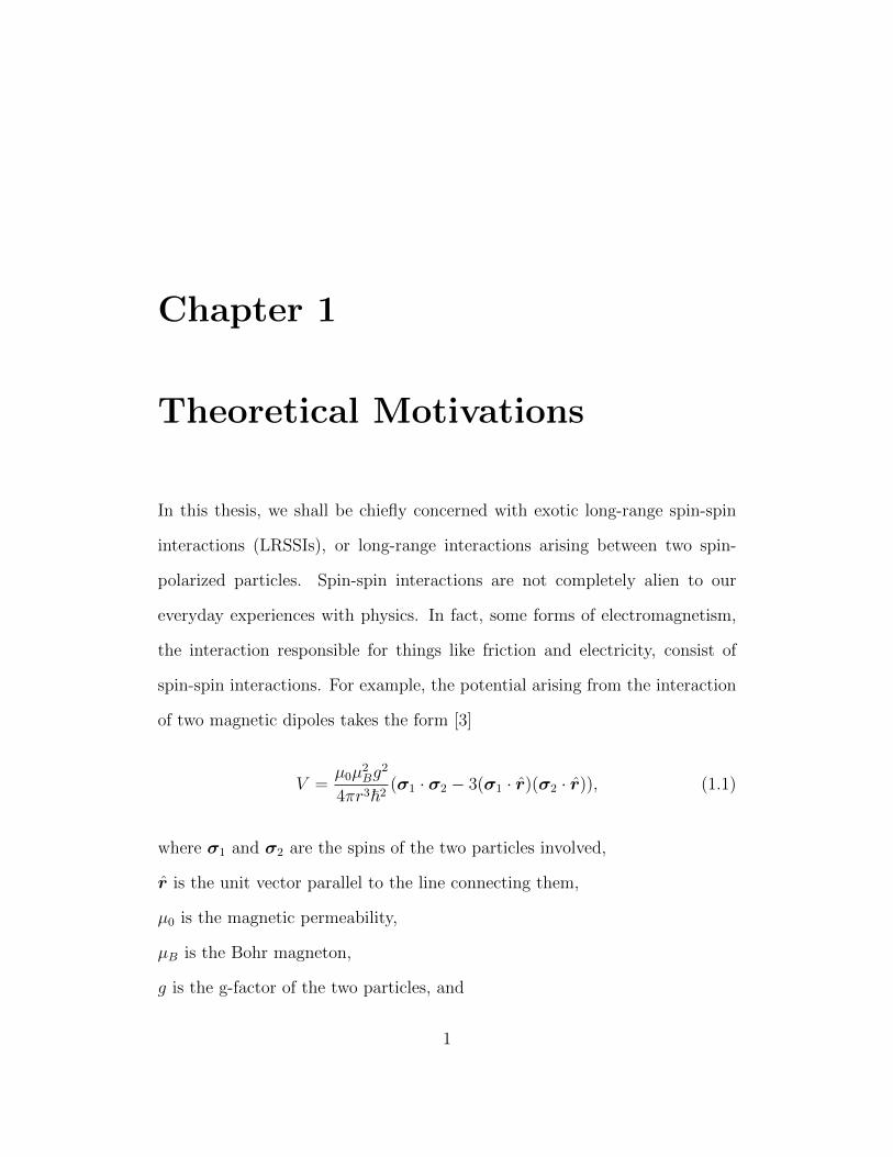
In this thesis, we shall be chiefly concerned with exotic long-range spin-spin
interactions (LRSSIs), or long-range interactions arising between two spin-
polarized particles. Spin-spin interactions are not completely alien to our
everyday experiences with physics. In fact, some forms of electromagnetism,
the interaction responsible for things like friction and electricity, consist of
spin-spin interactions. For example, the potential arising from the interaction
of two magnetic dipoles takes the form [3]
V =µ0µ
2Bg
2
4πr3~2(σ1 · σ2 − 3(σ1 · r)(σ2 · r)), (1.1)
where σ1 and σ2 are the spins of the two particles involved,
r is the unit vector parallel to the line connecting them,
µ0 is the magnetic permeability,
µB is the Bohr magneton,
g is the g-factor of the two particles, and
1
~ is Planck’s constant divided by 2π.
However, this thesis is not mainly concerned with standard spin-spin inter-
actions like Eq. 1.1 above. Instead, we are interested in experimentally probing
interactions that are completely removed from the four standard forces that
are established to exist in nature: gravity, the weak force, electromagnetism,
and the strong force, thus earning the label of “exotic” interactions. If ev-
idence for such interactions is found, these would constitute a fifth force of
nature. This would be an exciting form of new physics. The question remains,
however, why should we be concerned with exotic interactions? How did this
interest arise, and what is its relevance to the enterprise of physics research as
a whole? To answer this question, we must briefly look back to the history of
physics, especially in the last few decades.
1.1 Matter, Interactions, and the Emergence
of the Standard Model
Physics is a science studying the nature and behavior of matter in the uni-
verse. One of the most obvious aspects of studying the behavior of matter
is studying the possible interactions between different bodies of matter, such
as why a projectile seems to always drop back to the ground when a human
throws it up. Unsurprisingly, throughout its history, much of physics has been
concerned with the study of forces which give rise to these interactions. It
started with Newton, who came up with a rigorous theory that explained the
gravitational force. In the process, he discovered his Three Laws of Motion. In
2
the 19th century, one of the main scientific achievements was Maxwell’s unifi-
cation of electricity and magnetism. The resulting theory of electromagnetism
constitutes a second force in nature.
The progress of physics in the 20th century continued with the discoveries
of two pillars of modern physics: relativity and quantum mechanics. Both
of these theories were the subject of Einstein’s remarkable annus mirabilis of
1905, when he published papers on special relativity [4] and the photoelectric
effect [5]. In the next few years, Einstein developed the theory of general
relativity (GR) [6], which unified Newtonian gravity and special relativity.
Up to the current day, GR remains the only experimentally verified theory
that succesfully describes gravity. Meanwhile, Einstein’s argument for the
existence of light quanta in the photoelectric effect was vindicated in 1923,
with Compton’s scattering experiments that established the existence of the
photon, the force carrier for electromagnetism. Einstein’s argument, together
with Max Planck’s theory of quantized electromagnetic radiation (1900) and
Bohr’s initial model of the hydrogen atom (1913), eventually developed into
quantum mechanics (QM) in the 1920s, which has since been the predominant
paradigm in physics concerning interactions on a small scale.
This theme of unifying our understanding of different interactions contin-
ued in the next few decades. The discovery of QM led to interest in how
to unify it with the well-known theory of electromagnetism. In 1929, Pauli
and Heisenberg came up with the first attempts at quantum electrodynam-
ics (QED), a theory that described electromagnetism in the language of QM.
These first attempts came up short, in particular giving an infinite value for
3
the energy of the electron in its own electromagnetic field [7]. In the post-
World War II era physicists resumed work on QED, culminating with the
Nobel Prize in Physics being awarded for in 1965 to Feynman, Tomonaga, and
Schwinger for their development of the theory. QED was the first example of
a quantum field theory (QFT), a field theory that seeks to explain a force in
terms of quantum mechanics. The success of QED has been confirmed up to
the present day by experiments such as those measuring the electron g-factor,
the most recent of which found an agreement with the QED-calculated value
to almost a part per trillion [8].
Meanwhile, various events had led to the discovery of the weak force. Pauli
first proposed the neutrino (which he then called the “neutron”) in 1930 as a
way to explain the puzzling phenomenon of beta decay. In the following year,
Fermi created the first theory of beta decay that incorporated this new parti-
cle, the experimental confirmation of which did not occur until 1959. After the
success of QED, theorists sought to create a successful QFT that explained
the weak force. However, early attempts were unsuccessful, and many physi-
cists abandoned QFT in the 1960s in favor of doing research about Chew’s
S-matrix theory [7]. Thus when Glashow (1961) [9] and Weinberg and Salam
(1967) [10] found a way to combine electromagnetism and the weak interac-
tion in the framework of a field theory, now known as electroweak theory, it
was initially largely ignored until the 1970s. The trio’s work was eventually
awarded with the Nobel Prize in Physics in 1979. In this theory, intermediate
vector bosons were proposed as the force carriers for the weak force, consisting
of the W+,W−, and Z bosons. Direct evidence of their existence was obtained
4
in 1983 [11].
These advances in theoretical physics were accompanied and often initiated
by many groundbreaking experimental discoveries in particle physics. This
began in 1897 with the discovery of the electron by J.J. Thompson, followed
by Rutherford’s gold foil experiments that discovered the structure of the atom
in 1911. The fundamental question of how multiple positively charged protons
could remain in the nucleus of an atom without repelling each other resulted in
theorists positing the existence of the strong force. A string of discoveries over
the next few decades established that the proton and electron were not the
only elementary particles that existed: the positron (1931), neutron (1932),
muon and pion (1947), neutral kaons (1947), charged kaons (1949), and the
antiproton and antineutron (1955), among others [11].
Many of these particles had been predicted by theorists, such as the pion,
which was proposed by Yukawa in 1934 as the carrier particle of the strong
force. Some others, like the muon, were completely unexpected. To classify the
various new particles that had been discovered, in 1961 Gell-Mann came up
with a scheme known as the Eightfold Way, which classified particles based on
the properties of charge and strangeness. To explain the Eightfold Way, Gell-
Mann proposed the quark model in 1964. This theory proposed that baryons
and mesons are made up of elementary constituents known as quarks, and that
different kinds of elementary particles are the result of quarks with different
properties combining together. While there has been no direct observation of
free quarks, the existence of many new particles predicted by the theory has
been vindicated, most famously in the discovery of the J/ψ meson in 1974 by
5
Ting and Richter [12, 13]. These developments in the quark model led to Gell-
Mann and Harald Fritzsch proposing the theory of quantum chromodynamics
(QCD) in 1972, a QFT describing strong interacions. This theory posited
gluons as the force carrier for the strong force [14]. By the 1980s, the various
theories created and confirmed over the years had converged into the Standard
Model, which classified all the different elementary particles: leptons, quarks,
force carrier bosons, and the Higgs boson. The Standard Model’s latest tri-
umph is the experimental discovery of the Higgs boson at the Large Hadron
Collider (LHC) in 2012 [15, 16].
While it has been shown to be experimentally robust, the Standard Model
suffers from the limitation of requiring over 20 arbitrary parameters that are
theoretically unexplained and whose value is only obtainable by experiment.
We have seen from the history of physics that the quest of understanding
the interactions of matter in nature entails finding a theory to unify all four
forces, including harmonizing quantum mechanics and general relativity. The
Standard Model, therefore, falls short of being a “final theory” of physics and
invites opportunities for further investigation by physicists of this and future
generations. String theory is one of the most studied candidates for such a final
theory. It proposes that all matter consists of elementary microscopic strings,
and that the different particles are different modes of vibrations of such strings.
However, to this day there has been no experimental evidence for string theory,
and little realistic prospect of being able to perform an experiment capable of
probing it in the near future [17].
6
1.2 Origins of Exotic LRSSIs
1.2.1 The First Spin-Spin Interactions: The Strong-CP
Problem and Axions
Non-electromagnetic spin-spin interactions were first proposed due to the strong-
CP problem. This arose from the study of whether the laws of physics are sym-
metrical. The main fundamental discreet symmetries physicists are concerned
with are charge (C), parity (P), and time (T) symmetry. For a long time, it
was assumed that parity symmetry (which can be thought of as left- or right-
handedness) was self-evident in physics, and there was experimental evidence
that this was true for the case of strong, electromagnetic, and gravitational
interactions. However, in 1956 Lee and Yang proposed their theory of parity
violation in weak interactions [18], which was experimentally verified by Wu
the following year [19]. While parity symmetry had definitely been found to be
violated in Wu’s experiment, CP-symmetry (combining both charge and par-
ity symmetry) was not, and physicists began to wonder whether CP-symmetry
was a “true” symmetry in nature [11]. But in 1964 Cronin and Fitch found
evidence of CP violation in their experiments involving neutral kaons [20].
In contrast to the ample evidence for CP violation in the weak force, the
strong-CP problem emerges from the lack of evidence for such violations in the
strong force. The theory of QCD describing the strong force allows for a CP-
violating term in the QCD Lagrangian, which is characterized by a parameter
commonly denoted as θqcd. One of the best ways to probe θqcd is by measuring
the electric dipole moment dn of the neutron. A non-zero value would indicate
7
strong CP violation [21]. However, various searches have only found a value
of zero, with the latest one constraining it at [22]
|dn| < 2.9× 10⁻²⁶ e · cm, (1.2)
leading to the corresponding tight constraint
|θQCD| . 10−10, (1.3)
hence giving us the strong-CP problem. Various theories have been proposed
to explain the lack of such CP violation, with one of the most notable by
Roberto Peccei and Helen Quinn [23]. Peccei-Quinn theory proposes the exis-
tence of an axion field a functioning as a parameter of θQCD. This results in the
CP-violating term being canceled out from the QCD Lagrangian. The axion,
the new particle that mediates this field, is a pseudoscalar boson, which simply
means that it is a boson with spin-0 and odd parity.1 It is characterized by an
axion decay constant fa that determines the strength of the axion’s interaction
with Standard Model particles. For a large value of fa, the interaction will
be very weak, making the axion an example of a Weakly Interacting Sub-eV
Particle (WISP) [21].
In 1984, partly motivated by the proposal of not just axions, but also
other hypothetical particles such as familons, majorons, arions, and spin-1
antigravitons, Moody and Wilczek investigated the the potential forces that
could arise from the exchange from spin-0 bosons [24]. They investigated both
1A scalar boson is just a boson with spin-0 and even parity.
8
scalar and pseudoscalar bosons, and found spin-dependent potentials. Some
of these potentials were probed in an earlier generation of the current Hg-Cs
co-magnetometer apparatus at Amherst looking for spin-mass couplings [25],
as well as other experiments [26, 27]. More generally, as the axion is a possible
candidate for cold dark matter (CDM), much effort has been devoted to search
for it in both laboratory and astrophysical experiments [28].
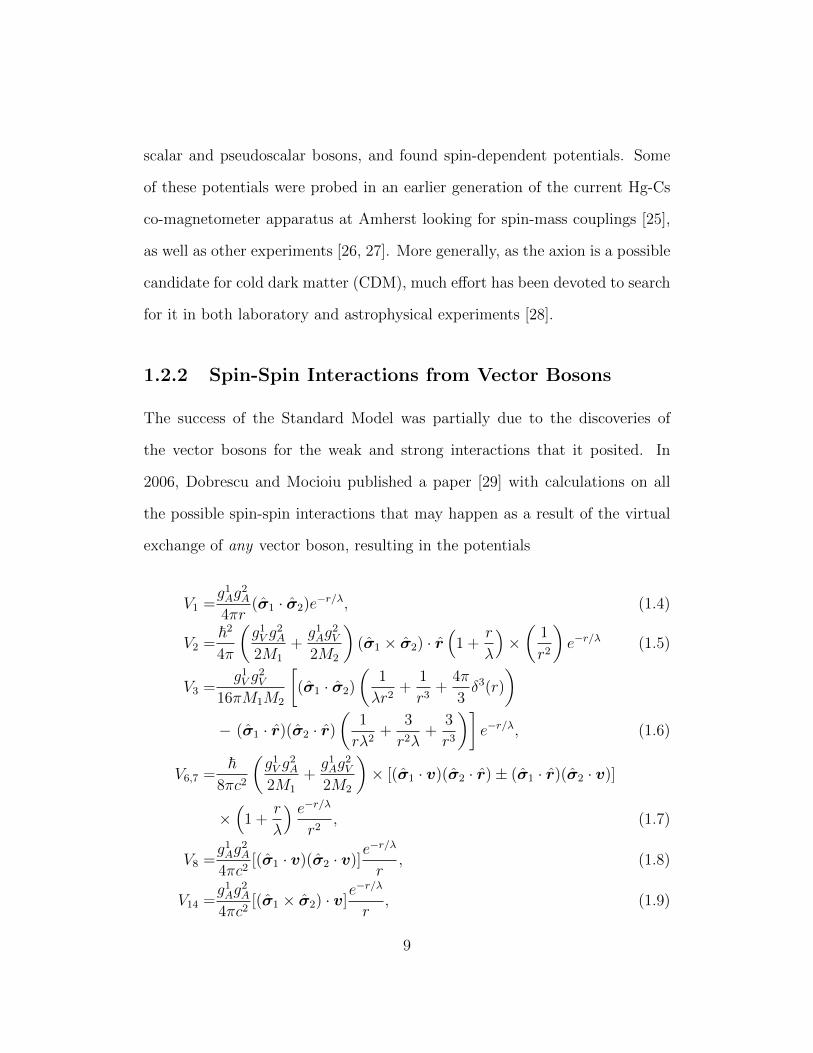
1.2.2 Spin-Spin Interactions from Vector Bosons
The success of the Standard Model was partially due to the discoveries of
the vector bosons for the weak and strong interactions that it posited. In
2006, Dobrescu and Mocioiu published a paper [29] with calculations on all
the possible spin-spin interactions that may happen as a result of the virtual
exchange of any vector boson, resulting in the potentials
V1 =g1Ag
2A
4πr(σ1 · σ2)e−r/λ, (1.4)
V2 =~2
4π
(g1V g
2A
2M1
+g1Ag
2V
2M2
)(σ1 × σ2) · r
(1 +
r
λ
)×(
1
r2
)e−r/λ (1.5)
V3 =g1V g
2V
16πM1M2
[(σ1 · σ2)
(1
λr2+
1
r3+
4π
3δ3(r)
)− (σ1 · r)(σ2 · r)
(1
rλ2+
3
r2λ+
3
r3
)]e−r/λ, (1.6)
V6,7 =~
8πc2
(g1V g
2A
2M1
+g1Ag
2V
2M2
)× [(σ1 · v)(σ2 · r)± (σ1 · r)(σ2 · v)]
×(
1 +r
λ
) e−r/λr2
, (1.7)
V8 =g1Ag
2A
4πc2[(σ1 · v)(σ2 · v)]
e−r/λ
r, (1.8)
V14 =g1Ag
2A
4πc2[(σ1 × σ2) · v]
e−r/λ
r, (1.9)
9
V15 =− g1V g
2V ~2
8πc3M1M2
× [(σ1 · (v × r))(σ2 · r) + (σ1 · r)(σ2 · (v × r))]
×(
3 +3r
λ+r2
λ2
)e−r/λ
r3, (1.10)
V16 =− ~8πc2
(g1V g
2A
2M1
+g1Ag
2V
2M2
)× [(σ1 · (v × r))(σ2 · v) + (σ1 · v)(σ2 · (v × r))]
×(
1 +r
λ
) e−r/λr2
, (1.11)
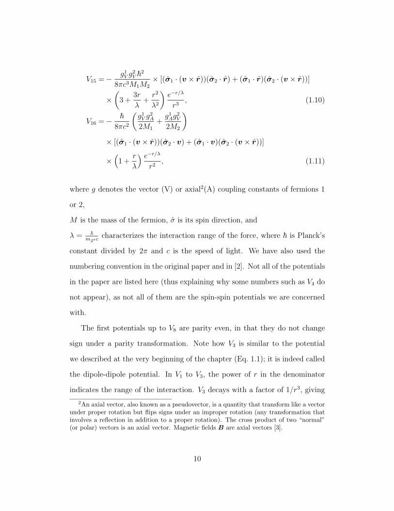
where g denotes the vector (V) or axial2(A) coupling constants of fermions 1
or 2,
M is the mass of the fermion, σ is its spin direction, and
λ = ~mZ′c
characterizes the interaction range of the force, where ~ is Planck’s
constant divided by 2π and c is the speed of light. We have also used the
numbering convention in the original paper and in [2]. Not all of the potentials
in the paper are listed here (thus explaining why some numbers such as V4 do
not appear), as not all of them are the spin-spin potentials we are concerned
with.
The first potentials up to V8 are parity even, in that they do not change
sign under a parity transformation. Note how V3 is similar to the potential
we described at the very beginning of the chapter (Eq. 1.1); it is indeed called
the dipole-dipole potential. In V1 to V3, the power of r in the denominator
indicates the range of the interaction. V3 decays with a factor of 1/r3, giving
2An axial vector, also known as a pseudovector, is a quantity that transform like a vectorunder proper rotation but flips signs under an improper rotation (any transformation thatinvolves a reflection in addition to a proper rotation). The cross product of two “normal”(or polar) vectors is an axial vector. Magnetic fields B are axial vectors [3].
10
a relatively short-ranged force compared to V1 and V2. This is important to
note as our experiment is mainly sensitive to long-range spin-spin interactions.
Note that V8 to V16 are velocity dependent potentials.
As our experiment has sensitivity towards the presence of spin-spin in-
teractions, with the help of a special method involving some geophysics and
calculations that will be detailed in section 1.4, it is possible to improve the
current bounds on these interactions.
1.3 What LRSSIs are Useful For
The spin-spin potentials discussed in Section 1.2 are general enough such that
our experiment is capable of probing any theory that proposes the existence of
any new vector gauge bosons. Such particles are sometimes termed Z ′ bosons,
to differentiate them from their Standard Model cousins.
1.3.1 Dark Photons and Massless Gauge Bosons
Some theorists have proposed the existence of gauge bosons that interact with
electrically charged particles through a phenomenon known as “kinetic mix-
ing” with the photon, often called “dark” photons as this coupling to ordinary
matter is very weak. The hypothesis of “hidden” or “dark” sectors of a rich ar-
ray of undiscovered particles not interacting with ordinary matter is commonly
found in various formulations of string theory. Different theories predict masses
for this hypothetical dark photon anywhere from several MeV or GeV to sub-
eV levels. There are even theories that propose gauge bosons that kinetically
11
mix with other Standard Model gauge bosons such as the Z boson that me-
diates the electroweak force, giving us “dark” Z ′ bosons [30]. Consequences
of the coupling of dark Z ′ bosons to ordinary matter include exotic atomic
parity violations and new decay channels for the Higgs boson [31]. Many ex-
periments have already or are being carried out to probe for dark particles
at various mass scales, such as the electron beam dump experiments at the
Stanford Linear Accelerator Center (SLAC) [32], the High Energy Accelerator
Research Organization in Japan (KEK), and the Laboratoire de l’accelerateur
linaire (LAL) in Orsay, France [33]. In electron beam dump experiments like
these, a very intense beam of electrons is directed at a fixed target in order
to probe the extremely weak interactions between dark photons and ordinary
matter. However, no evidence for them has been found yet.
The question of the existence of completely massless gauge bosons has
also been explored. Again, kinetic mixing occurs and allows some very weak
interactions with Standard Model fermions. Their presence would affect phe-
nomena like muon and Higgs boson decay, Big Bang nucleosynthesis (the for-
mation of atomic nuclei during the Big Bang), and star cooling. They are also
considered a possible dark matter candidate [34].
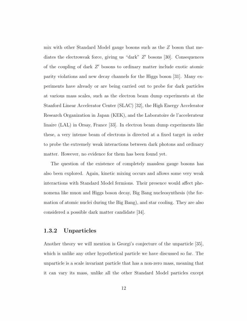
1.3.2 Unparticles
Another theory we will mention is Georgi’s conjecture of the unparticle [35],
which is unlike any other hypothetical particle we have discussed so far. The
unparticle is a scale invariant particle that has a non-zero mass, meaning that
it can vary its mass, unlike all the other Standard Model particles except
12
the photon (which has zero mass). Although its mass is undefined, they can
still be described by an energy scale Λ, scaling dimension d and dimensionless
coupling constant cA. It turns out that the exchange of an unparticle results
in a spin-spin interaction in the long-range limit [36], namely
Vu = −c2A
4√πΓ(d+ 1/2)Γ(2(d− 1))
(2π)2dΓ(d− 1)Γ(2d)(σ1 · σ2)×
(~cr
)(~cΛr
)2d−2
, (1.12)
where Γ is the gamma function. Thus our experiment is also capable of probing
for the existence of the unparticle with certain values of d.
1.3.3 Other Proposals
LRSSIs are also relevant in probing for torsion gravity, a variant of the Einstein-
Cartan theory of gravity, which is an alternative theory of gravity to general
relativity that relaxes certain assumptions [37]. In general, the search for Z ′
bosons is a cornerstone of many contemporary research programs in physics,
from high-energy experiments at large particle accelerators all the way to low-
energy table-top experiments such as ours. Many other theories have proposed
Z ′ bosons at varying energies, such as E6 Grand Unified Theories [38], Little
Higgs models [39], topcolor models [40], Kaluza-Klein theory [41], just to name
a few. This abundance of experimental and theoretical efforts clearly indicates
that the hunt for Z’ bosons is considered one of the most promising paths for
encountering new physics.
13
1.4 Geophysical Methods to Constrain LRSSIs
In this section, we shall discuss the method by which we extrapolate the results
from our apparatus (as well as other relevant experiments) to bounds on exotic
spin-spin interactions. This method was first described in our two earlier
papers [1, 2].
1.4.1 Basic Concept
There are three ingredients needed to investigate spin-spin interactions (espe-
cially ones that are very weak, as we have seen in Section 1.2): first is a large
amount of spin-polarized particles that serves as the source of the interaction
- the more the better as the interaction will be stronger and more visible.
Secondly, one needs a relatively smaller spin-polarized source of particles that
can be monitored in the lab, serving as the “test charge” affected by the main
source. Finally, one needs a way to modify the extent of the spin-spin interac-
tion, as otherwise we would be stuck with a measurement value that contains
the spin-spin interaction signal plus the value of any other physical processes
we apply to the apparatus (such as a magnetic field in our case), and be unable
to separate these two components. By changing the extent of the spin-spin
interaction while keeping these background effects constant, we can subtract
the values measured from the two settings to isolate the spin-spin interaction
signal. In practice, this modification is done by changing the polarization of
the main source or the lab apparatus.
For the main spin source, many previous experiments have used a local
14
source consisting of a mass of spin-polarized particles placed a short distance
from the test apparatus. For example, an experiment at the University of
Washington investigating e−−e− (electron-electron) couplings used four rings
each consisting of Alnico and SmCo magnets positioned inside their torsion
balance apparatus [42]. Another experiment at Princeton University investi-
gated n−n (neutron-neutron) couplings using a source of spin-polarized 3He
atoms placed 50 cm from their co-magnetometer apparatus [43]. An advan-
tage of such local sources is that it is easy to reverse the polarization, and the
short distance between the source and the test apparatus also allows probing
of shorter-ranged forces. However, the number of electrons in a local labora-
tory source is limited to ∼1022 neutrons or ∼1025 electrons due to practical
constraints.
In our method, we use the spin-polarized electrons inside the Earth as our
source, thinking of them as interacting with the spins in the co-magnetometer
in our lab. There are ∼1049 unpaired electrons inside the Earth, and ∼1042 are
spin-polarized. This is 17 orders of magnitude more than a typical laboratory
source. A trade-off is that these particles are located several thousand of
kilometers away, as opposed to tens of centimeters - a difference of 7 orders of
magnitude. This makes our method primarily sensitive to interactions that fall
off over 1/rn with n ≤ 2, because with n = 3, we lose 21 orders of magnitude,
losing our numerical advantage. This is why this thesis is primarily concerned
with long-ranged (or low mass) spin-spin interactions, and we are not very
sensitive to V3 which has n = 3. All of the other potentials in Eqs. 1.4-1.11
have n = 1 or 2 with the exception of V15, which has never been experimentally
15
bounded before. As the spin-polarization of the Earth’s electrons depends
on the Earth’s magnetic field, the geographical location of the experiments
will be significant, depending on the functional form of the potential we are
bounding. Additionally, an important consequence of using the Earth as a
spin source is that due to the Earth’s rotation, electrons at different depths
will have different velocities relative to each other, and also to our apparatus
at the surface. This makes it possible for us to probe for velocity-dependent
interactions, something difficult to do with local laboratory spin sources.
A disadvantage of Earth spin sources, however, is that it is not possible to
change its polarization. Nevertheless, it is possible to change the orientation
of the detector instead, which gives the same effect. Hence experiments which
collect data in two different measuring positions (for example by mounting
the apparatus on a rotating table), such as in [44–46] as well as our own
apparatus [47] can be analyzed with our method.
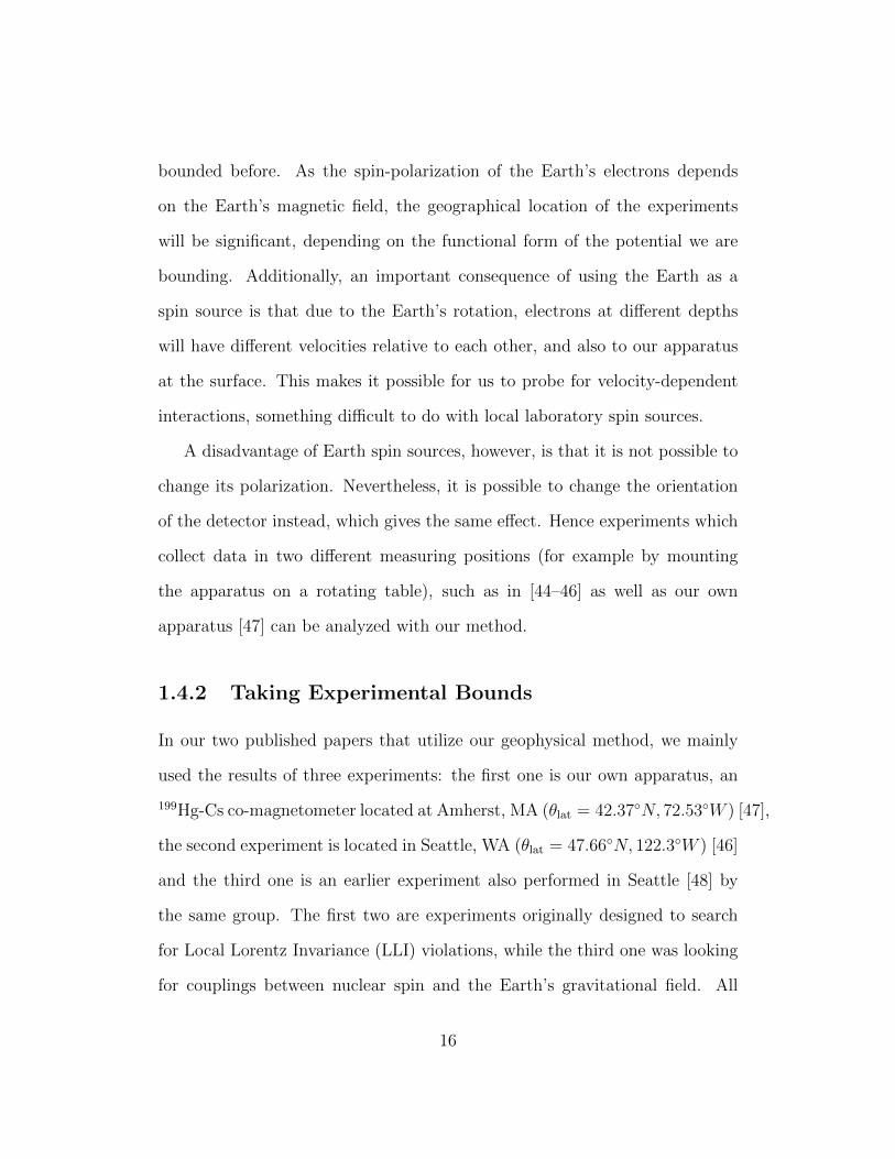
1.4.2 Taking Experimental Bounds
In our two published papers that utilize our geophysical method, we mainly
used the results of three experiments: the first one is our own apparatus, an
199Hg-Cs co-magnetometer located at Amherst, MA (θlat = 42.37N, 72.53W ) [47],
the second experiment is located in Seattle, WA (θlat = 47.66N, 122.3W ) [46]
and the third one is an earlier experiment also performed in Seattle [48] by
the same group. The first two are experiments originally designed to search
for Local Lorentz Invariance (LLI) violations, while the third one was looking
for couplings between nuclear spin and the Earth’s gravitational field. All
16
returned null results, and thus can be used to constrain LRSSIs.
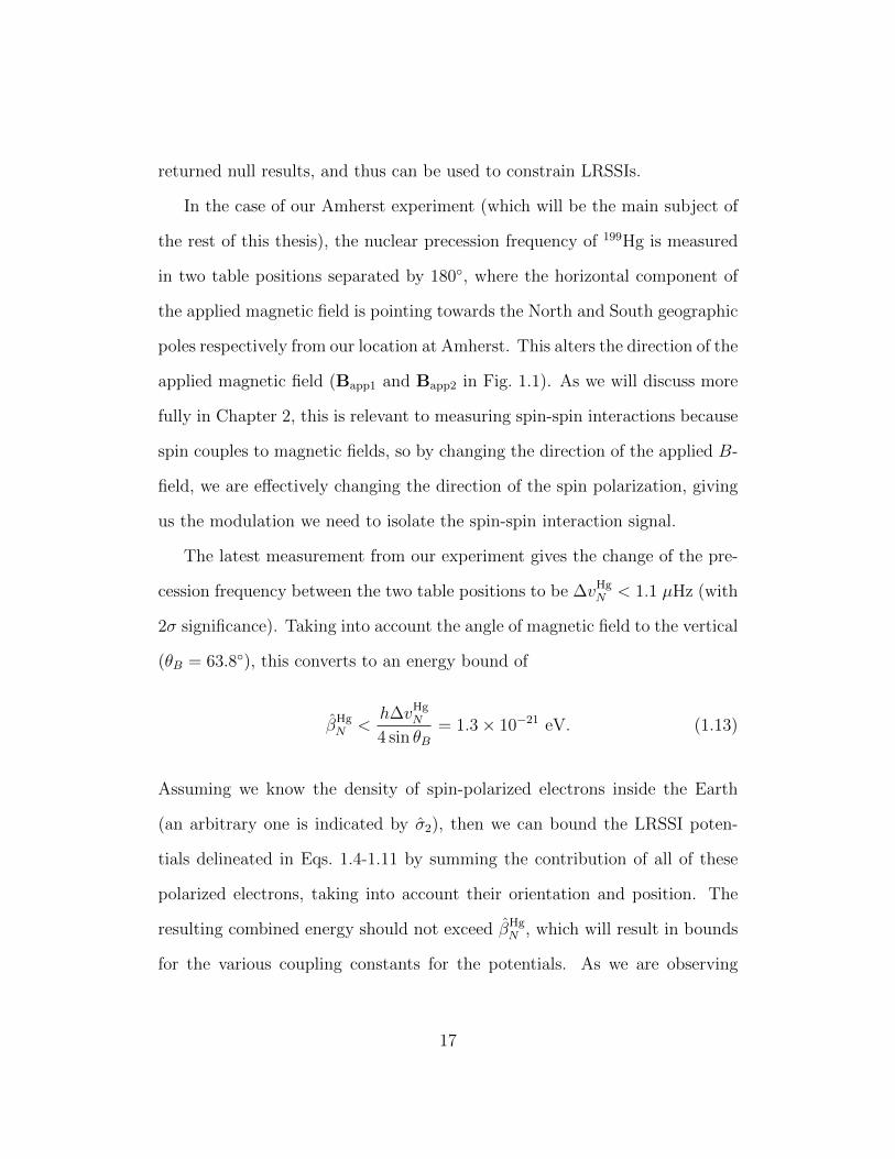
In the case of our Amherst experiment (which will be the main subject of
the rest of this thesis), the nuclear precession frequency of 199Hg is measured
in two table positions separated by 180, where the horizontal component of
the applied magnetic field is pointing towards the North and South geographic
poles respectively from our location at Amherst. This alters the direction of the
applied magnetic field (Bapp1 and Bapp2 in Fig. 1.1). As we will discuss more
fully in Chapter 2, this is relevant to measuring spin-spin interactions because
spin couples to magnetic fields, so by changing the direction of the applied B-
field, we are effectively changing the direction of the spin polarization, giving
us the modulation we need to isolate the spin-spin interaction signal.
The latest measurement from our experiment gives the change of the pre-
cession frequency between the two table positions to be ∆vHgN < 1.1 µHz (with
2σ significance). Taking into account the angle of magnetic field to the vertical
(θB = 63.8), this converts to an energy bound of
βHgN <
h∆vHgN
4 sin θB= 1.3× 10⁻²¹ eV. (1.13)
Assuming we know the density of spin-polarized electrons inside the Earth
(an arbitrary one is indicated by σ2), then we can bound the LRSSI poten-
tials delineated in Eqs. 1.4-1.11 by summing the contribution of all of these
polarized electrons, taking into account their orientation and position. The
resulting combined energy should not exceed βHgN , which will result in bounds
for the various coupling constants for the potentials. As we are observing
17
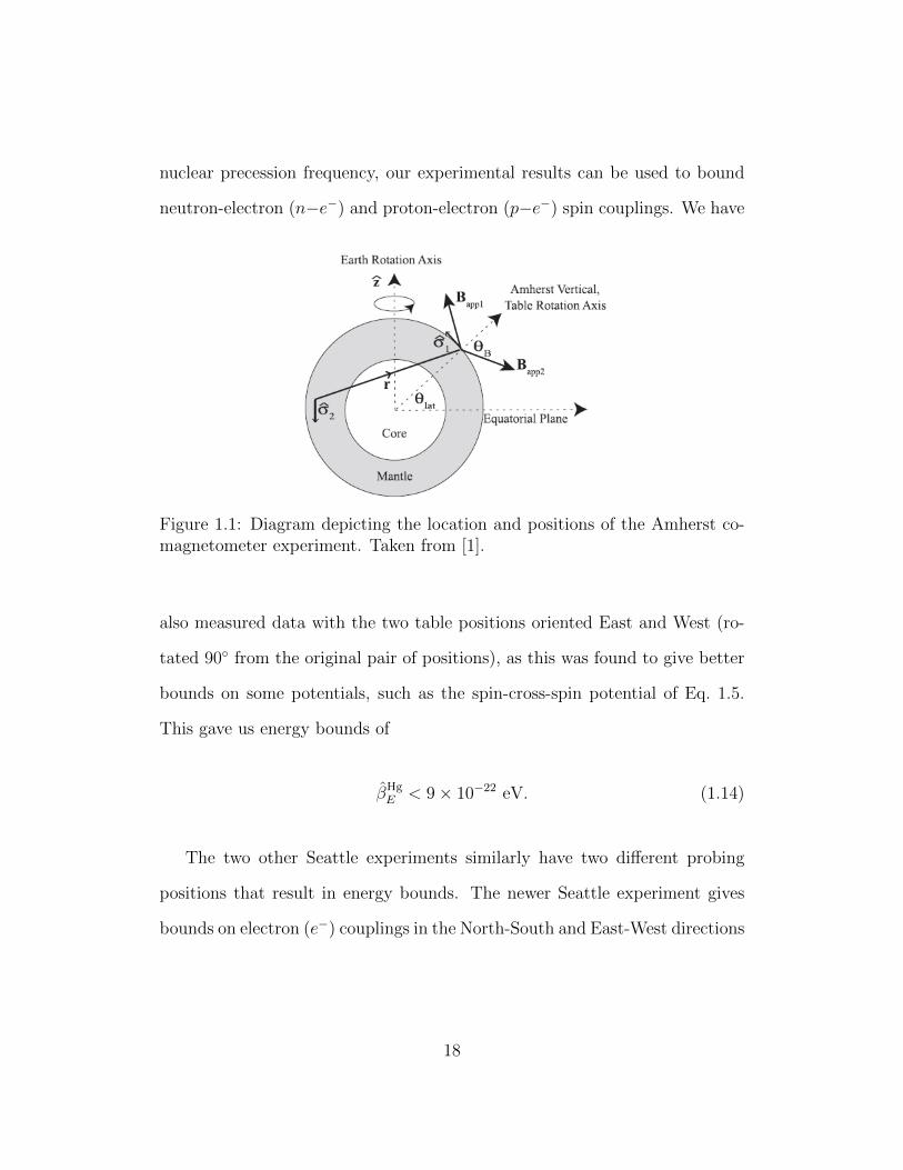
nuclear precession frequency, our experimental results can be used to bound
neutron-electron (n−e−) and proton-electron (p−e−) spin couplings. We have
Figure 1.1: Diagram depicting the location and positions of the Amherst co-magnetometer experiment. Taken from [1].
also measured data with the two table positions oriented East and West (ro-
tated 90 from the original pair of positions), as this was found to give better
bounds on some potentials, such as the spin-cross-spin potential of Eq. 1.5.
This gave us energy bounds of
βHgE < 9× 10⁻²² eV. (1.14)
The two other Seattle experiments similarly have two different probing
positions that result in energy bounds. The newer Seattle experiment gives
bounds on electron (e−) couplings in the North-South and East-West directions
18
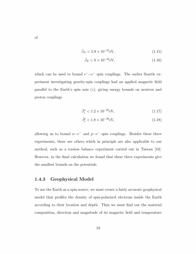
of
βN < 5.9× 10⁻²¹eV, (1.15)
βE < 8× 10⁻²²eV, (1.16)
which can be used to bound e−−e− spin couplings. The earlier Seattle ex-
periment investigating gravity-spin couplings had an applied magnetic field
parallel to the Earth’s spin axis (z), giving energy bounds on neutron and
proton couplings
βnz < 1.2× 10⁻²⁰eV, (1.17)
βpz < 1.8× 10⁻²⁰eV, (1.18)
allowing us to bound n−e− and p−e− spin couplings. Besides these three
experiments, there are others which in principle are also applicable to our
method, such as a torsion balance experiment carried out in Taiwan [44].
However, in the final calculation we found that these three experiments give
the smallest bounds on the potentials.
1.4.3 Geophysical Model
To use the Earth as a spin source, we must create a fairly accurate geophysical
model that profiles the density of spin-polarized electrons inside the Earth
according to their location and depth. Thus we must find out the material
composition, direction and magnitude of its magnetic field and temperature
19
profile everywhere inside the Earth, as these all influence the density of spin-
polarized electrons. The profile of Earth’s magnetic field is readily available
using the World Magnetic Model [49], while the temperature profile of the
Earth’s mantle is also widely understood among geophysicists [50]. Finding
out the proportions of different minerals and metals at different depths is not
as straightforward, however, and the details of our model are given in [1].
Our model ignores the possibility of spin-polarized electrons located inside the
Earth’s core, density functional theories indicate that there are no unpaired
electron spins in the core due to the high temperatures and pressures [51]. This
is a conservative assumption as this will only weaken the bounds obtained from
the model. The result of our model is a spin-density map of the entire Earth,
a cross-section of which is shown in Fig. 1.2.
1.4.4 Calculating the Bounds
To obtain the actual bounds, we fit the data in our model to find the following
three functions:
B(r′, θ′, φ′), the Earth’s magnetic field,
T (r′), the temperature of the Earth, and
ρ(r′), the electron density,
where r′, θ′, and φ′ are parameters of a spherical coordinates system with an
origin at the center of the Earth’s core. We then calculate Vtotal, the sum of
contributions by all of the geoelectrons to the potential, by performing a 3-
dimensional integral over the Earth’s volume from the core-mantle boundary
20
Figure 1.2: A cross-section from the spin-polarized electron density plot weobtained from our geophysical model. Taken from [1].
21
(RCM) to the surface (RS), namely
Vtotal =
∫ 2π
0
∫ π
0
∫ RS
RCM
r′2 sin θ′ × ρ(r′)× 2µBB(r′, θ′, φ′)
kBT (r′)
× V (r(r′, θ′, φ′),v(r′, θ′, φ′)) dr′dθ′dφ′, (1.19)
where µB is the Bohr magneton,
kB is Boltzmann’s constant, and
V (r(r′, θ′, φ′)v(r′, θ′, φ′)) is the function of the potential being bounded (taken
from Eqs. 1.4-1.11), with
r(r′, θ′, φ′) = r′A − r′, (1.20)
where r′A is the vector designating the location of Amherst or Seattle, and
r′ is the vector designating the location of the geoelectron. For velocity-
dependent potentials (Eqs. 1.7-1.11), we also need to calculate the velocity
function
v(r′, θ′, φ′) = v′A − v′, (1.21)
with
v′A = Ω× r′A, (1.22)
v′ = Ω× r′, (1.23)
Ω =2π
tday
z, (1.24)
22
where tday is the length of time of a sidereal day and z is the vector parallel to
the rotation axis of the Earth. For non-velocity-dependent potentials then we
would only have V (r(r′, θ′, φ′)) in Eq. 1.19. These integrals are numerically
calculated using Mathematica for different ranges λ (or different boson masses
mZ′ , since λ ∝ 1/mZ′). To ensure the veracity of such a complicated integral,
we perform the calculation using two slightly different methods: in the first,
we numerically integrate thin shells of tens of km thickness and manually add
them together, while in the second method we instruct Mathematica to directly
calculate the full integral. We further ensured the robustness of our bounds
by repeating the calculations with double the density of electrons in the lower
mantle and taking the worse bound, to take into account any changes in the
electron density (or alternatively, disagreements between geologists about our
electron density profile).
Fig. 1.3 is an example plot of our bounds, in this case for V1. In our two
previous papers, the bounds we established on all of the investigated poten-
tials were at least 1-2 orders of magnitude better than previous experimental
methods. In the case of velocity-dependent potentials, none of them had been
bounded before, with the exception of V8, which we improved in the long-range
limit by 30 orders of magnitude compared to the previous bound [52].
1.5 Improving the Results
The next step in our research is naturally to improve the bounds calculated
using our geophysical method. A conceptually simple way to do this would be
23
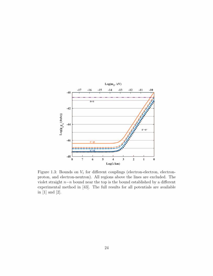
Figure 1.3: Bounds on V1 for different couplings (electron-electron, electron-proton, and electron-neutron). All regions above the lines are excluded. Theviolet straight n−n bound near the top is the bound established by a differentexperimental method in [43]. The full results for all potentials are availablein [1] and [2].
24
to shift the geographic location of our experiment where the Earth’s surface
magnetic field is stronger and more parallel to the surface. We estimated in [1]
that our experiment would be twice as sensitive to LRSSIs were it conducted
in a region near the equator (such as southern Thailand). A more practical
suggestion, however, would be to improve the apparatus itself. As we will
discuss in Ch. 2, the Amherst experiment was limited by AC light shift. We
hope to overcome this by implementing a new optical geometry that hopefully
will give at least an order of magnitude improvement on our bounds. Besides
this, we also anticipate results from other co-magnetometer experiments [53,
54] that will hopefully produce improved energy bounds on spin-couplings to
various fermions that can be applied to our model, resulting in improvements
in bounds for LRSSIs.
1.6 Summary
To summarize this chapter, we have explored how the search for spin-spin inter-
actions is a natural development of the general quest undertaken by physicists
to understand all the different interactions between matter in nature. We have
described the specific spin-spin interaction potentials that we are looking for
and shown how our new geophysical method is able to transform bounds from
several different spin-sensitive experiments into bounds for these LRSSIs. In
the following chapters, we shall turn to the more specific case of our own ap-
paratus at Amherst College and discuss our efforts to continue the search for
LRSSIs by improving the experiment.
25
Chapter 2
Physics of the Experiment
In this chapter, we shall discuss the physics of the experimental apparatus
in the Hunter Lab at Amherst College. Some basic facts have already been
mentioned in Chapter 1: the apparatus is a co-magnetometer, or in other
words, a device capable of measuring a magnetic field, and it uses two different
types of gas cells to perform this task (hence the “co”): mercury (Hg) and
cesium (Cs). Since we have not yet worked with the Hg cells, most of the
discussion in this chapter will be focused on Cs. However, most of the physics
of optical pumping and probing also applies to Hg. The main differences are
the lifetime, precession frequency, and the frequency of the light needed. These
differences are all associated with mercury’s different atomic structure. We will
delve deeper into the physics of how our magnetometers work, both of the past
generation as well as the planned future generation of the experiment. This
will allow us to explain why we believe the proposed changes will improve the
experiment’s sensitivity.
26
We shall henceforth refer to the past generation of the apparatus as the
Gen I magnetometer, while the newly proposed apparatus will be referred to
as the Gen II magnetometer. We shall constantly note any relevant differences
between Gen I and Gen II, in order to gain a comprehensive picture of how
the latter should be a definite improvement on the former.
2.1 Basic Concept
Spin is an intrinsic property of particles in nature. It is a particle’s inherent
angular momentum, and as an intrinsic property it cannot be altered or taken
away, similar to mass and charge [55]. Spin is not a classical property like
orbital angular momentum, and despite having both magnitude and direction,
in quantum mechanics a spin state is not represented by an ordinary vector,
but instead by a mathematical object called a spinor. Still, in some contexts
such as ours a classical picture may remain useful, for example in representing
spin by a pseudovector S. If we are only talking about the direction of the
spin, we can also represent it using the vector σ, where
Sz = mz~σ, (2.1)
where mz is the spin quantum number along a particular axis of quantization
(z-axis in this case). When we talk about spin-polarized particles, we simply
mean that a large number of particles have their spins σi oriented along a
certain direction of polarization, resulting in a net polarization.
In order to be able to detect spin-spin interactions in a way that is useful
27
for the geophysical method explained in Chapter 1, one needs to be able to
create a source of spin-polarized particles in the lab, and also keep track of
the spins. To accomplish the latter, in this experiment we take advantage of
the fact that spin couples to magnetic fields, as expressed in the Hamiltonian
H = −µ ·Bapp = −γS ·Bapp, (2.2)
where µ is the magnetic dipole moment, Bapp is an applied magnetic field,
γ is the gyromagnetic ratio of the particle and S represents the spin of the
particle. If exotic spin-spin interactions exist, then such interactions would be
added on to the Hamiltonian:
H ′ = −γS ·Bapp + V (S), (2.3)
where V (S) is a potential (such as one of those defined in Eq. 1.4-1.11) which
depends on the spin S of the particle. As both terms in H ′ contain S, we can
rework the equation by pulling out S. The details would depend on the actual
form of V (S). For example, let us take the potential V1, defined previously in
Eq. 1.4 as taking the form of
V1 = K(SL · SE), (2.4)
where K is a variable containing variables r and λ and also other constants
as needed, and we use the notation SL for a spin in the lab and SE for a spin
inside the Earth. Note that we have converted the σ spin vectors appearing
28
in the original Eq. 1.4 into S. Then Eq. 2.3 becomes
H ′ = −γSL ·Bapp +K(SL · SE)
= −γSL ·(
Bapp −K
γSE
)= µ ·Beff. (2.5)
So if V1 exists, then it would have the effect of altering the magnetic field
experienced by the particle. Similar manipulation can be done to the other
potentials to arrive at the same conclusion. Thus we can search for LRSSIs by
subjecting the particle to a fixed magnetic field Bapp and pointing our appara-
tus to different directions in order to look for any changes in the magnetic field
which may be caused by any of these exotic interactions. It is essential that
one is able to change the direction of Bapp in order to modulate the spin-spin
interaction signal. Otherwise we would be stuck with a certain value of the
measured effective magnetic field and not know how much of it is due to Bapp
and how much of it is due to LRSSIs.
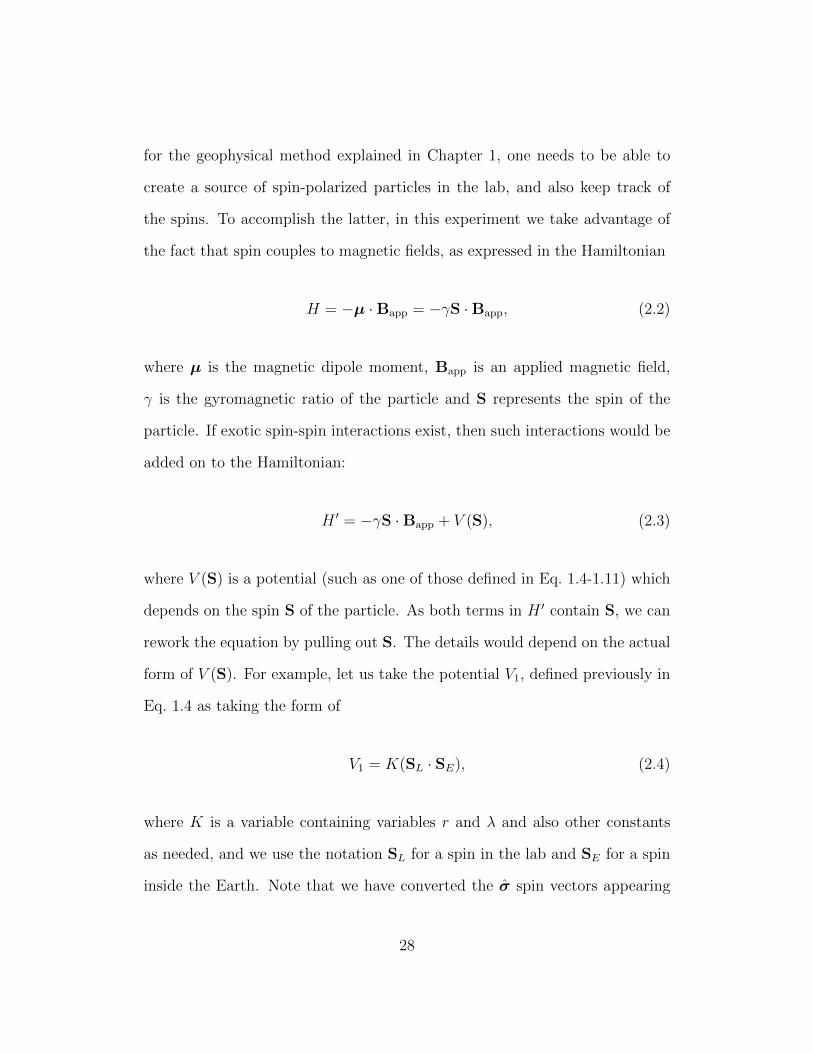
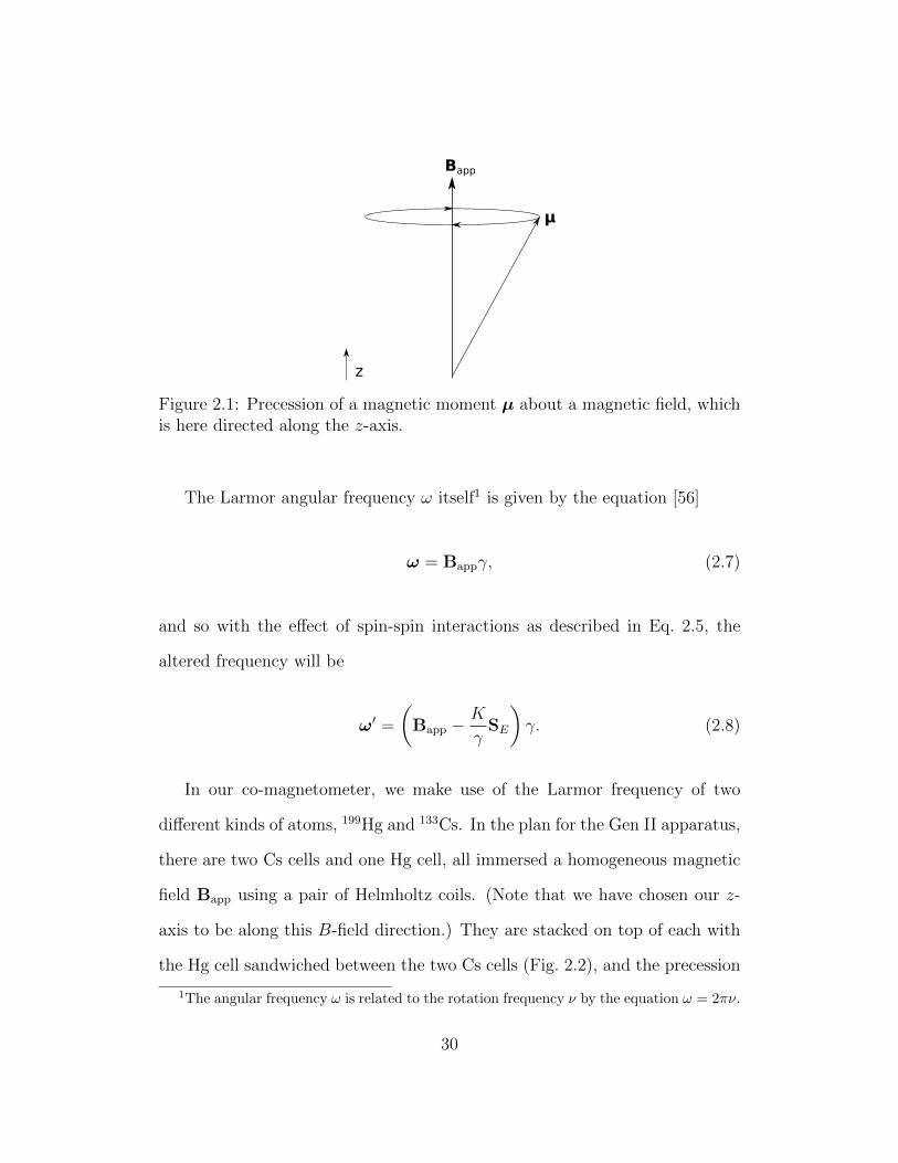
To monitor the magnetic field, we observe the Larmor frequency of the
particle, which is the natural frequency at which the magnetic moment µ
precesses in the magnetic field Bapp, as seen in Fig. 2.1. This precession is
caused by a torque
τ = µ×Bapp, (2.6)
which in the figure points out of the page.
29
Bapp
μ
z
Figure 2.1: Precession of a magnetic moment µ about a magnetic field, whichis here directed along the z-axis.
The Larmor angular frequency ω itself1 is given by the equation [56]
ω = Bappγ, (2.7)
and so with the effect of spin-spin interactions as described in Eq. 2.5, the
altered frequency will be
ω′ =
(Bapp −
K
γSE
)γ. (2.8)
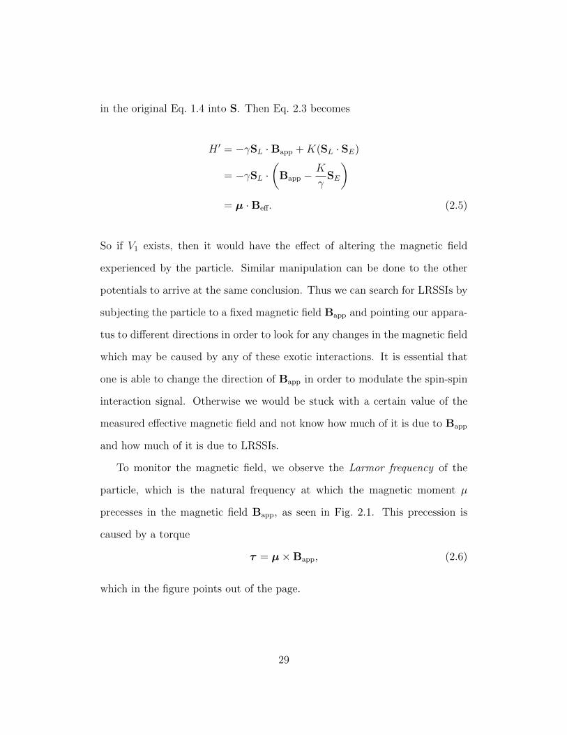
In our co-magnetometer, we make use of the Larmor frequency of two
different kinds of atoms, 199Hg and 133Cs. In the plan for the Gen II apparatus,
there are two Cs cells and one Hg cell, all immersed a homogeneous magnetic
field Bapp using a pair of Helmholtz coils. (Note that we have chosen our z-
axis to be along this B-field direction.) They are stacked on top of each with
the Hg cell sandwiched between the two Cs cells (Fig. 2.2), and the precession
1The angular frequency ω is related to the rotation frequency ν by the equation ω = 2πν.
30
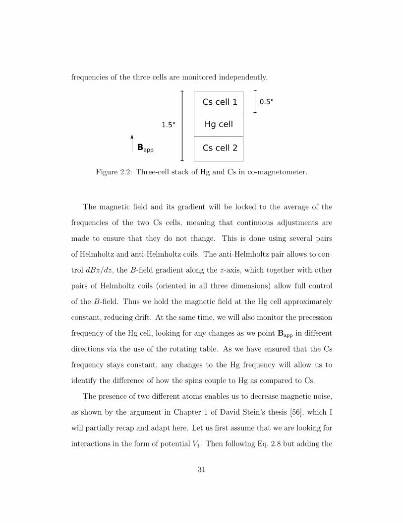
frequencies of the three cells are monitored independently.
Bapp
Cs cell 1
Cs cell 2
Hg cell
0.5"
1.5"
Figure 2.2: Three-cell stack of Hg and Cs in co-magnetometer.
The magnetic field and its gradient will be locked to the average of the
frequencies of the two Cs cells, meaning that continuous adjustments are
made to ensure that they do not change. This is done using several pairs
of Helmholtz and anti-Helmholtz coils. The anti-Helmholtz pair allows to con-
trol dBz/dz, the B-field gradient along the z-axis, which together with other
pairs of Helmholtz coils (oriented in all three dimensions) allow full control
of the B-field. Thus we hold the magnetic field at the Hg cell approximately
constant, reducing drift. At the same time, we will also monitor the precession
frequency of the Hg cell, looking for any changes as we point Bapp in different
directions via the use of the rotating table. As we have ensured that the Cs
frequency stays constant, any changes to the Hg frequency will allow us to
identify the difference of how the spins couple to Hg as compared to Cs.
The presence of two different atoms enables us to decrease magnetic noise,
as shown by the argument in Chapter 1 of David Stein’s thesis [56], which I
will partially recap and adapt here. Let us first assume that we are looking for
interactions in the form of potential V1. Then following Eq. 2.8 but adding the
31
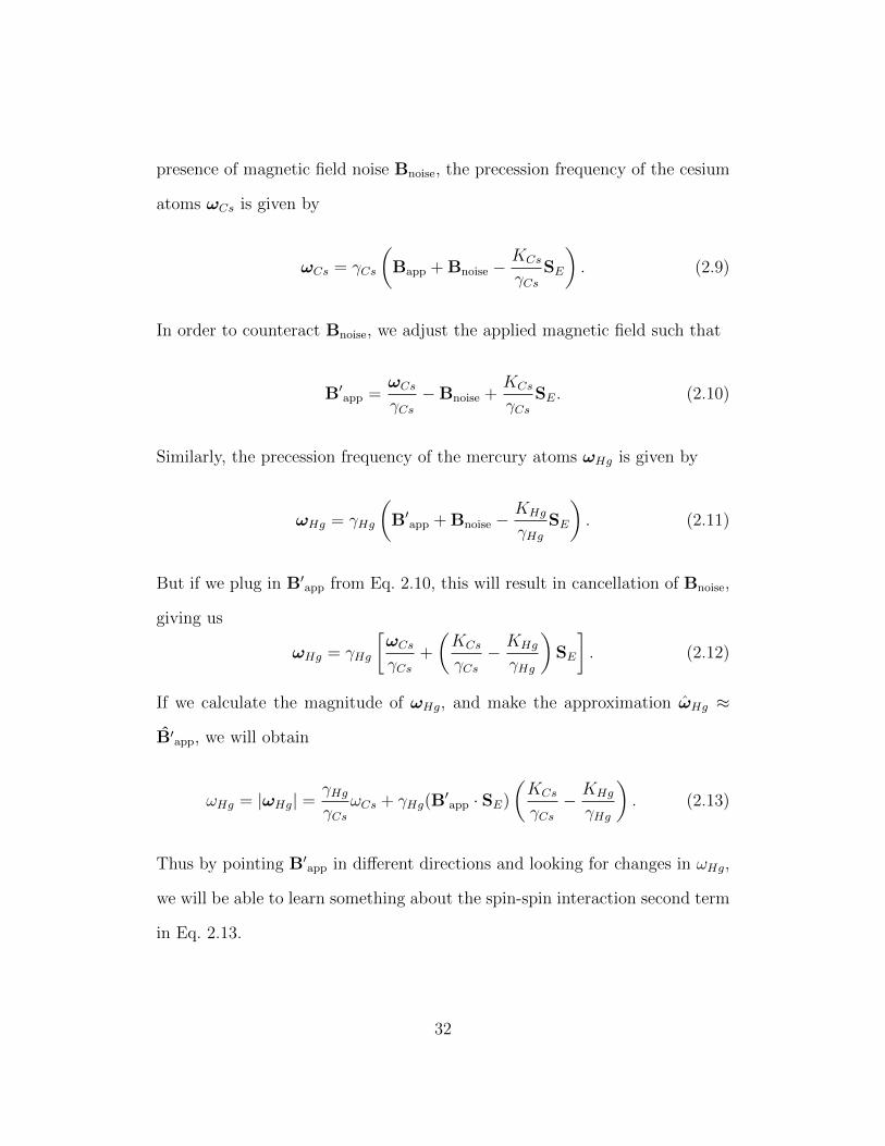
presence of magnetic field noise Bnoise, the precession frequency of the cesium
atoms ωCs is given by
ωCs = γCs
(Bapp + Bnoise −
KCs
γCsSE
). (2.9)
In order to counteract Bnoise, we adjust the applied magnetic field such that
B′app =ωCsγCs−Bnoise +
KCs
γCsSE. (2.10)
Similarly, the precession frequency of the mercury atoms ωHg is given by
ωHg = γHg
(B′app + Bnoise −
KHg
γHgSE
). (2.11)
But if we plug in B′app from Eq. 2.10, this will result in cancellation of Bnoise,
giving us
ωHg = γHg
[ωCsγCs
+
(KCs
γCs− KHg
γHg
)SE
]. (2.12)
If we calculate the magnitude of ωHg, and make the approximation ωHg ≈
B′app, we will obtain
ωHg = |ωHg| =γHgγCs
ωCs + γHg(B′app · SE)
(KCs
γCs− KHg
γHg
). (2.13)
Thus by pointing B′app in different directions and looking for changes in ωHg,
we will be able to learn something about the spin-spin interaction second term
in Eq. 2.13.
32
2.2 Optical Pumping
How does one look for changes in the precession frequencies ωHg and ωCs?
While all of the atoms are precessing together in the constant applied magnetic
field, they are all out of phase with each other, and thus we cannot probe the
entire system. Our first step is to make all the atoms in a cell have a net
spin polarization. This is accomplished by optical pumping, in which we apply
electromagnetic radiation tuned at a certain resonant frequency to the atoms.
The resonant light transfers its angular momentum to the atoms. For the
case of Cs, we use circularly polarized light from a diode laser tuned to the
62S1/2 → 62P1/2 transition, also known as the D1 transition. This corresponds
to a frequency of about 894 nm, and this transition is used for both the pump
and probe lasers. We shall now elaborate further both of the Cs transitions
and also the details of how optical pumping works.
2.2.1 The Cs D1 Transition
Cesium is an alkali metal, i.e., it comes from the first column of the periodic
table, and thus has one valence electron. Cesium-133 is its only stable isotope,
possessing a total nuclear angular momentum I = 7/2. In quantum mechanics,
the possible hyperfine quantum numbers F are defined by
F = J + I (2.14)
33
where the magnitude of F can take on the values
|J − I| < F < J + I. (2.15)
The 62S1/2 → 62P1/2 transition has J = 1/2 for both states, and so we can
only have F = 3 or F = 4, resulting in only two hyperfine levels for both
the ground and excited states. These two levels are easy to resolve and work
with, making this an attractive transition for optical pumping as we have only
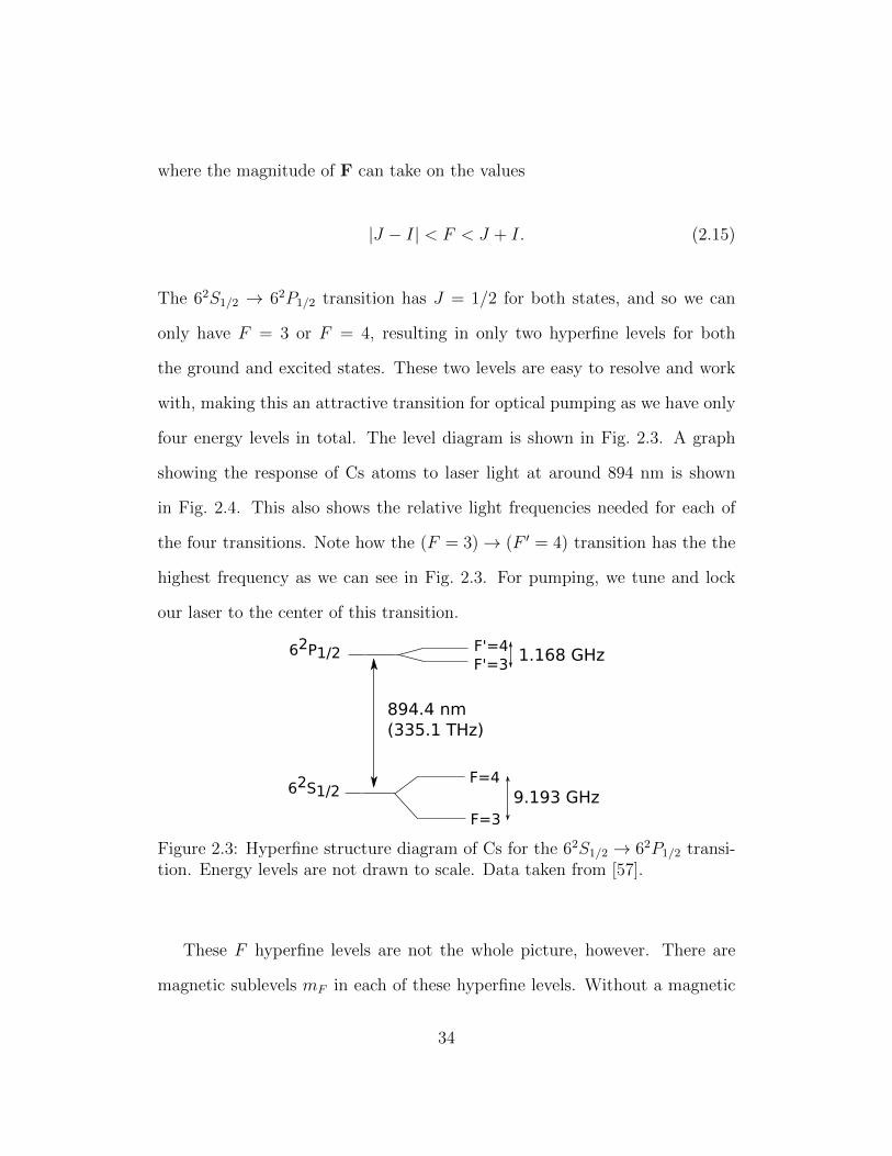
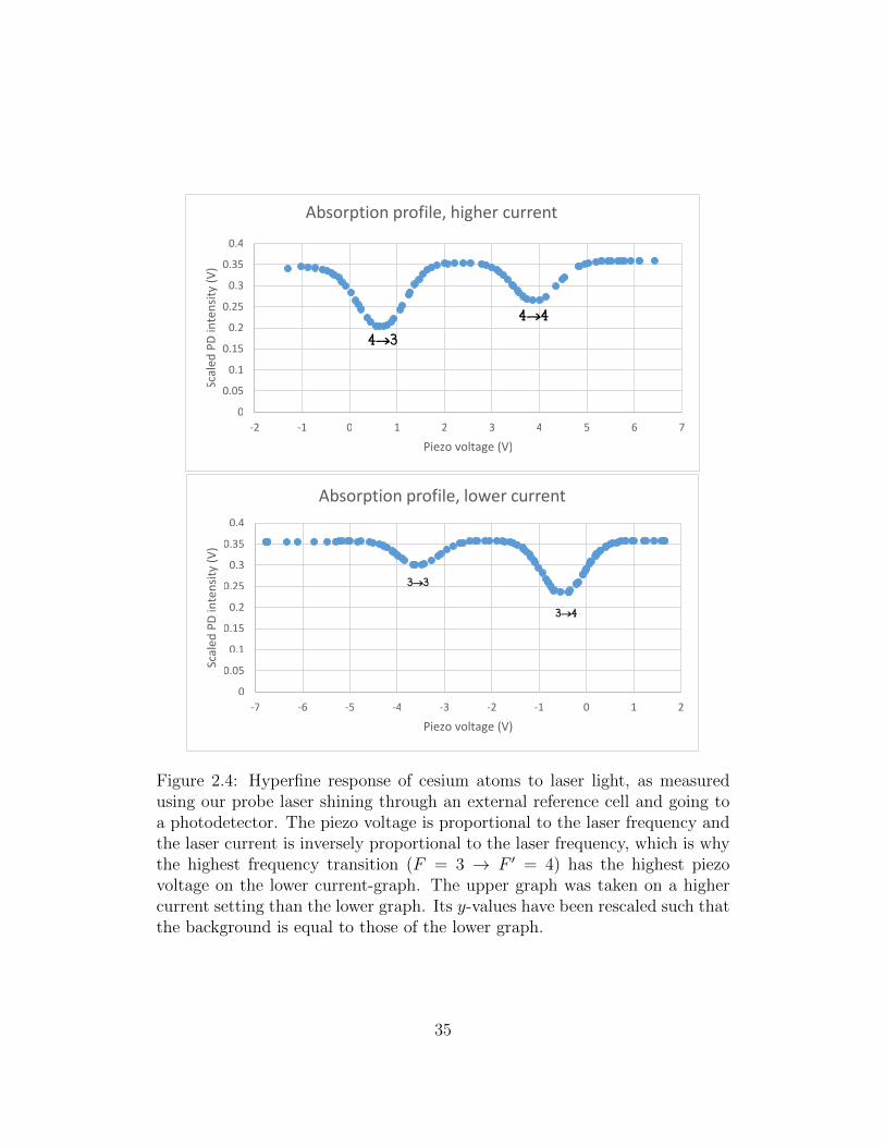
four energy levels in total. The level diagram is shown in Fig. 2.3. A graph
showing the response of Cs atoms to laser light at around 894 nm is shown
in Fig. 2.4. This also shows the relative light frequencies needed for each of
the four transitions. Note how the (F = 3)→ (F ′ = 4) transition has the the
highest frequency as we can see in Fig. 2.3. For pumping, we tune and lock
our laser to the center of this transition.
62P1/2
62S1/2
F'=3F'=4
F=3
F=4
894.4 nm(335.1 THz)
1.168 GHz
9.193 GHz
Figure 2.3: Hyperfine structure diagram of Cs for the 62S1/2 → 62P1/2 transi-tion. Energy levels are not drawn to scale. Data taken from [57].
These F hyperfine levels are not the whole picture, however. There are
magnetic sublevels mF in each of these hyperfine levels. Without a magnetic
34
0
0.05
0.1
0.15
0.2
0.25
0.3
0.35
0.4
-2 -1 0 1 2 3 4 5 6 7
Scal
ed P
D in
ten
sity
(V
)
Piezo voltage (V)
Absorption profile, higher current
4>34>4
0
0.05
0.1
0.15
0.2
0.25
0.3
0.35
0.4
-7 -6 -5 -4 -3 -2 -1 0 1 2
Scal
ed P
D in
ten
sity
(V
)
Piezo voltage (V)
Absorption profile, lower current
3>4
3>3
Figure 2.4: Hyperfine response of cesium atoms to laser light, as measuredusing our probe laser shining through an external reference cell and going toa photodetector. The piezo voltage is proportional to the laser frequency andthe laser current is inversely proportional to the laser frequency, which is whythe highest frequency transition (F = 3 → F = 4) has the highest piezovoltage on the lower current-graph. The upper graph was taken on a highercurrent setting than the lower graph. Its y-values have been rescaled such thatthe background is equal to the lower graph’s.
34
Figure 2.4: Hyperfine response of cesium atoms to laser light, as measuredusing our probe laser shining through an external reference cell and going toa photodetector. The piezo voltage is proportional to the laser frequency andthe laser current is inversely proportional to the laser frequency, which is whythe highest frequency transition (F = 3 → F ′ = 4) has the highest piezovoltage on the lower current-graph. The upper graph was taken on a highercurrent setting than the lower graph. Its y-values have been rescaled such thatthe background is equal to those of the lower graph.
35
field, the energies of these sublevels are degenerate. However, in the pres-
ence of a magnetic field, as in our experiment, the Zeeman effect breaks the
degeneracy, giving different energies for the sublevels [57].
2.2.2 A Basic Two-Level System
σ+
θ
x
y
s
B
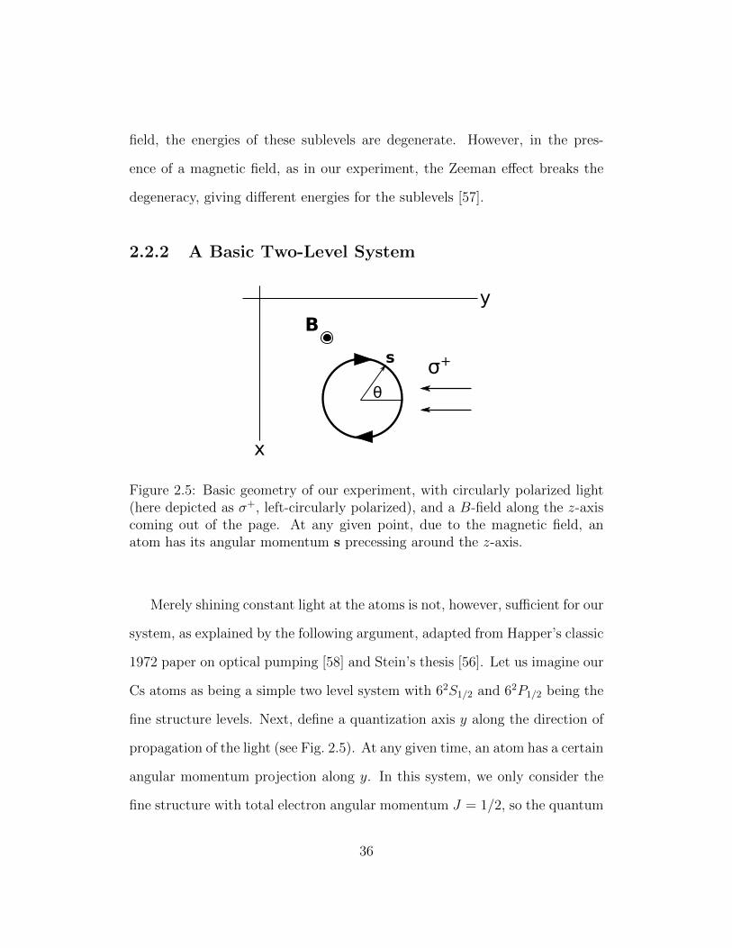
Figure 2.5: Basic geometry of our experiment, with circularly polarized light(here depicted as σ+, left-circularly polarized), and a B-field along the z-axiscoming out of the page. At any given point, due to the magnetic field, anatom has its angular momentum s precessing around the z-axis.
Merely shining constant light at the atoms is not, however, sufficient for our
system, as explained by the following argument, adapted from Happer’s classic
1972 paper on optical pumping [58] and Stein’s thesis [56]. Let us imagine our
Cs atoms as being a simple two level system with 62S1/2 and 62P1/2 being the
fine structure levels. Next, define a quantization axis y along the direction of
propagation of the light (see Fig. 2.5). At any given time, an atom has a certain
angular momentum projection along y. In this system, we only consider the
fine structure with total electron angular momentum J = 1/2, so the quantum
36
state can be expressed in the form
|ψ〉 = A |+y〉+B |−y〉 , (2.16)
where A and B describe the probability amplitudes for the atom being in the
state mj = +1/2 or mj = −1/2 respectively. Let us assume that we are
shining left-circularly polarized light (commonly denoted as σ+). An atom
which already has mj = +1/2, i.e. its angular momentum is completely along
the direction of +y with A = 1, cannot accommodate additional angular
momentum, so it cannot absorb photons from the laser light and will remain
in the ground state. In contrast, atoms with mj = −1/2 (B = 1) can absorb a
photon, which will excite it to the state 62P1/2 with mj = 1/2. The majority
of atoms will be in some intermediate state
|ψ〉 =1
2(1 + eiθ) |+y〉+
1
2(1− eiθ) |−y〉 , (2.17)
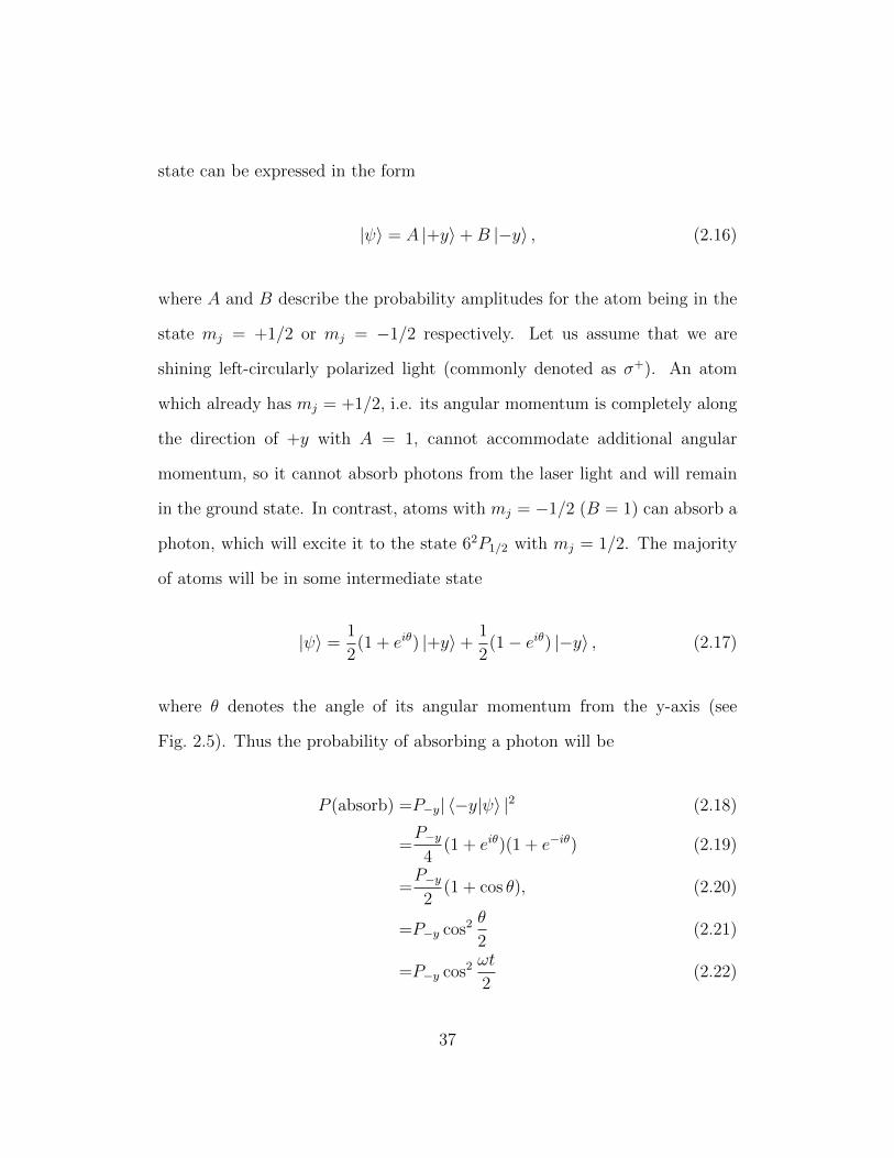
where θ denotes the angle of its angular momentum from the y-axis (see
Fig. 2.5). Thus the probability of absorbing a photon will be
P (absorb) =P−y| 〈−y|ψ〉 |2 (2.18)
=P−y
4(1 + eiθ)(1 + e−iθ) (2.19)
=P−y
2(1 + cos θ), (2.20)
=P−y cos2 θ
2(2.21)
=P−y cos2 ωt
2(2.22)
37
where P−y denotes the probability of absorption when A = 1. In the last line,
we use the relation θ = ωt, as the spins precess at the Larmor frequency. To
properly calculate P−y, one would have to work out the necessary quantum
mechanics using density matrices [58] or rate equations [59], which are beyond
the reach of a typical undergraduate curriculum, but for our purposes, it does
not matter what value P−y takes as long as it is non-zero. If, say, P−y is a
small fraction, then the left-circularly polarized light would still be absorbed
by the atom, although it might take a long time before a coherent polarization
occurs. The sinusoidal term in Eq. 2.22 creates a modulation in the absorption
in the light, which will in turn result in a modulation in the intensity of
the transmitted light. But because the system is initially unpolarized, each
individual atom has its own values for A and B and they will absorb photons
at different times. Also, excited atoms may collide with the walls of the cell
and relax back to the ground state. Relaxation to the ground state also occurs
through spontaneous emission. In the end, we have a collection of atoms
being excited and decaying all at different times, resulting in only a very small
net angular momentum polarization along the direction of the pump. This is
insufficient for our needs, and so we introduce modulation to our pump light.
2.2.3 Modulated Pump Light: the Bell-Bloom Magne-
tometer
Optical pumping using modulated pump light was first suggested by Dehmelt
and performed by Bell and Bloom in 1957 [60]. To understand how it works,
38
consider again Fig. 2.5.2 The Cs cell is immersed in a uniform magnetic field
B = B0z, and left-circularly polarized pump light σ+ is directed along the
y-axis. The light is amplitude-modulated (using square waves) at a frequency
ωm, while the Larmor frequency of the Cs is ωCs as before. Now assume
that ωm = ωCs, and at time t = t0 light strikes the cell.3 Some atoms will
have a quantum state with A = 1 (from Eq. 2.16), and so they are already
spin-polarized in the direction we want. All the other atoms, which have
0 ≤ A < 1, have some probability of getting pumped to the excited state.
At t = t0 + 2π/ωCs, light will strike the cell again. Atoms which had been
excited at t = t0 will now have A = 1, and cannot be affected by the light.
But all the other atoms, including those which did not get excited, will now
“get a second chance” to be excited, so to speak, and some will indeed end
up being excited, adding to the total spin polarization of the system. At the
same time the polarization obtained at t = t0 remains. The same process
continues at t = t0 + 4π/ωCs, t = t0 + 6π/ωCs, and so on. Assuming no other
depolarizing forces are present, eventually all of the atoms will be precessing
together in phase with the same polarization. In reality, the polarization will
increase until a certain value where the rate of pumping is equal to the rate of
the depolarization.
If the pumping laser is turned off, then the atoms’ spins will keep precessing
together for a while, but with a decay constant of T2, which we call the lifetime
of the cell. T2 is affected by several factors, such as the design of the cell,
2The following explanation is inspired by Chapter 1 of Budker and Kimball’s book onoptical magnetometry [61].
3For simplicity, let us assume that all of the photons in a single oscillation of the pumplight are absorbed in an instant instead of over some non-zero amount of time.
39
whether an anti-relaxation coating is used for the cell walls, and also atoms
colliding with each other and causing spin exchange which de-excites them.
The longer T2 is, the more time we have to observe the cell before the spin
polarization disappears.
Atoms which are de-excited may decay from the 62P1/2(F ′ = 3) state to
either the 62S1/2(F = 3) or 62S1/2(F = 4) state. As we only pump using a
single laser at the F = 3 → F ′ = 4 transition, the 62S1/2(F = 4) state is
technically a “dark” state, unreachable by our lasers. However, in practice
enough natural spin-exchange collisions happen such that many atoms in the
dark state decay into the lowest ground state (62S1/2(F = 3)), such that there
is always a sizable fraction of the atoms in this state, allowing us to freely
pump and let the atoms decay multiple times.
We can also think about the system as being a driven harmonic oscillator,
with the natural frequency Ωn = ωCs and the driving frequency Ωd = ωm.
The largest amplitude of oscillation will occur when Ωn = Ωd. This is also
convenient as we can introduce the idea of a damping force, corresponding to
the various forces that cause the decay of the spin polarization. In order for
the driven harmonic oscillator to achieve a significant amplitude of oscillation,
the damping force has to be much smaller then the driving force.
2.3 Optical Probing
In order to monitor the actual precession caused by the optical pumping, we use
a separate diode laser which we call the probe laser. Unlike the circularly po-
40
larized pump laser, the probe laser is linearly polarized and is not modulated,
but shining constantly. It is also tuned about 3 GHz off the F = 4→ F ′ = 3
transition. The laser light passes through the pumped Cs cells in an orthog-
onal direction to the pump beam, and picked up by photodetectors on the
other side. Optical probing in this manner allows us to observe the precession
frequencies of our atoms by a process known as optical rotation.
2.3.1 Light Polarization and Optical Rotation
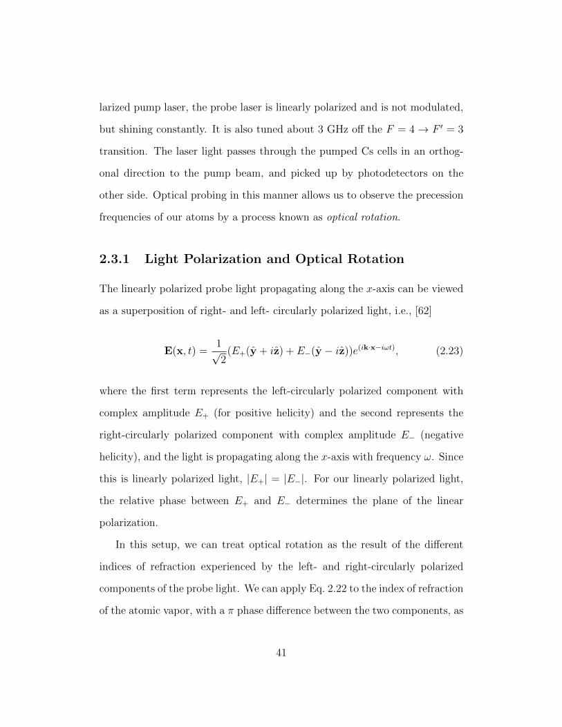
The linearly polarized probe light propagating along the x-axis can be viewed
as a superposition of right- and left- circularly polarized light, i.e., [62]
E(x, t) =1√2
(E+(y + iz) + E−(y − iz))e(ik·x−iωt), (2.23)
where the first term represents the left-circularly polarized component with
complex amplitude E+ (for positive helicity) and the second represents the
right-circularly polarized component with complex amplitude E− (negative
helicity), and the light is propagating along the x-axis with frequency ω. Since
this is linearly polarized light, |E+| = |E−|. For our linearly polarized light,
the relative phase between E+ and E− determines the plane of the linear
polarization.
In this setup, we can treat optical rotation as the result of the different
indices of refraction experienced by the left- and right-circularly polarized
components of the probe light. We can apply Eq. 2.22 to the index of refraction
of the atomic vapor, with a π phase difference between the two components, as
41
the absorption of the left-circularly polarized component will be the greatest
when the right circularly component is at the smallest, and vice versa. But
before we can do this, we have to first derive the formula for the index of
refraction.
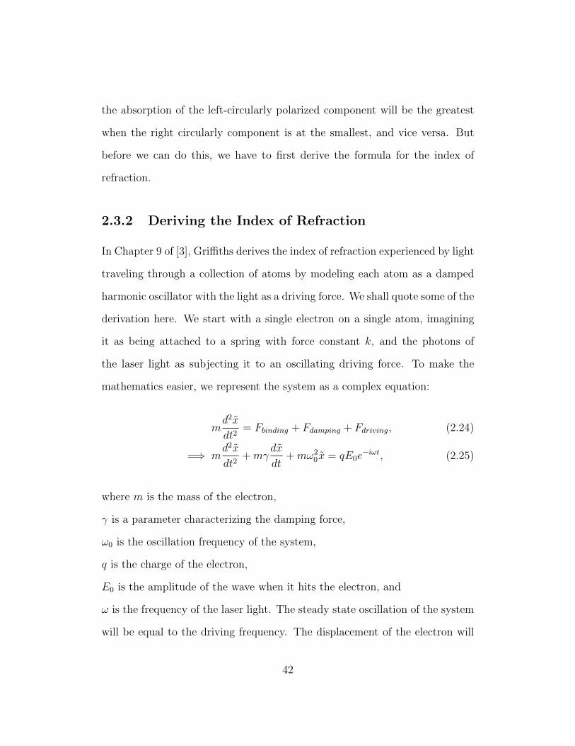
2.3.2 Deriving the Index of Refraction
In Chapter 9 of [3], Griffiths derives the index of refraction experienced by light
traveling through a collection of atoms by modeling each atom as a damped
harmonic oscillator with the light as a driving force. We shall quote some of the
derivation here. We start with a single electron on a single atom, imagining
it as being attached to a spring with force constant k, and the photons of
the laser light as subjecting it to an oscillating driving force. To make the
mathematics easier, we represent the system as a complex equation:
md2x
dt2= Fbinding + Fdamping + Fdriving, (2.24)
=⇒ md2x
dt2+mγ
dx
dt+mω2
0x = qE0e−iωt, (2.25)
where m is the mass of the electron,
γ is a parameter characterizing the damping force,
ω0 is the oscillation frequency of the system,
q is the charge of the electron,
E0 is the amplitude of the wave when it hits the electron, and
ω is the frequency of the laser light. The steady state oscillation of the system
will be equal to the driving frequency. The displacement of the electron will
42
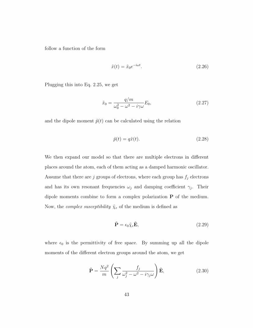
follow a function of the form
x(t) = x0e−iωt. (2.26)
Plugging this into Eq. 2.25, we get
x0 =q/m
ω20 − ω2 − iγωE0, (2.27)
and the dipole moment p(t) can be calculated using the relation
p(t) = qx(t). (2.28)
We then expand our model so that there are multiple electrons in different
places around the atom, each of them acting as a damped harmonic oscillator.
Assume that there are j groups of electrons, where each group has fj electrons
and has its own resonant frequencies ωj and damping coefficient γj. Their
dipole moments combine to form a complex polarization P of the medium.
Now, the complex susceptibility χe of the medium is defined as
P = ε0χeE, (2.29)
where ε0 is the permittivity of free space. By summing up all the dipole
moments of the different electron groups around the atom, we get
P =Nq2
m
(∑j
fjω2j − ω2 − iγjω
)E, (2.30)
43
from which we can extract the value of χe.
We then take plane wave solution of the wave equation
E(x, t) = E0ei(kx−ωt) (2.31)
= E0ei((k+iξ)x−ωt), (2.32)
= E0e−ξxei(kx−ωt) (2.33)
where we have assumed a beam propagating in the x-direction (as in our
apparatus) and broken up complex wave number k into its real and imaginary
parts, k = k+ iξ. Eq. 2.33 shows that the wave is attenuated, and its intensity
will be proportional to e−2ξx. Thus we can define an absorption coefficient α
by
α = 2ξ (2.34)
and also calculate the index of refraction n by the formula
n =ck
ω. (2.35)
Using the formula for χe and the relation
k = ω√µ0ε0(1 + χe) (2.36)
and doing some approximations along the way, eventually we will get
n = 1 +Nq2
2mε0
∑j
fj(ω2j − ω2)
(ω2j − ω2)2 + γ2
jω2, (2.37)
44
α =Nq2ω
mε0c
∑j
fjγj(ω2
j − ω2)2 + γ2jω
2, (2.38)
where N is the number of atoms per volume.
Now that we have derived the index of refraction, we can apply it to our
system as we outlined in Sec. 2.3.1. Referring back to the analogy of a photon
striking an electron, we must also take into account that in our system, the
probability of such an event happening is affected by the probabilities of light
absorption expressed in Eq. 2.22. When the polarization is pointing along the
−x direction, only the left-circularly polarized component can be absorbed,
and when it is along the +x direction, only the right-circularly polarized com-
ponent can be absorbed. Thus, we have to multiply sinusoidal terms that
are π out of phase to the index of refraction experienced by left- and right-
circularly polarized components of the probe light, i.e.
n+ = cos2
(Ωt
2
)(1 +
Nq2
2mε0
∑j
fj(ω2j − ω2)
(ω2j − ω2)2 + γ2
jω2
), (2.39)
n− = cos2
(Ωt+ π
2
)(1 +
Nq2
2mε0
∑j
fj(ω2j − ω2)
(ω2j − ω2)2 + γ2
jω2
)
= sin2
(Ωt
2
)(1 +
Nq2
2mε0
∑j
fj(ω2j − ω2)
(ω2j − ω2)2 + γ2
jω2
). (2.40)
This oscillation in the indices of refraction causes the optical rotation.
2.3.3 Implications of the Index of Refraction
We can plot α and n from Eq. 2.38 about a resonant frequency ωj in order to
see how the behavior of the light around the line center of the atomic transition
45
frequency. We assume that the other resonances are far away, and so only one
of the terms in the summation survives. As ω is very close to ωj, we make the
approximation that ωj ≈ ω, and so (ω + ωj) ≈ 2ωj. Thus we obtain
n = 1 +Nq2
2mε0
(fj(ω
2j − ω2)
(ω2j − ω2)2 + γ2
jω2
)(2.41)
=⇒ n− 1 ≈ Nq2
2mε0
(fj(2ωj)
2(ωj − ω)
(2ωj)2(ωj − ω)2 + γ2jω
2
)(2.42)
≈ Nq2
mε0
(2fj∆ω
4(∆ω)2 + γ2j
)(2.43)
and
α =Nq2
2mε0c
(ωfjγj
(ω2j − ω2)2 + γ2
jω2
)(2.44)
≈ Nq2
2mε0c
(ωfjγj
(2ωj)2(ωj − ω)2 + γ2jω
2
)(2.45)
≈ Nq2
2mε0cωj
(fjγj
4(∆ω)2 + γ2j
), (2.46)
where ∆ω = ωj − ω.
Using Mathematica and setting fj = 1 and γj = Nq2/2mε0 = 1 for simplic-
ity,4 we obtain the plots shown in Fig. 2.6. Notice that with increasing ∆ω,
the absorption of the light decays faster than the index of refraction which
causes optical rotation. This is the reason why we tune 3 GHz off resonance:
to avoid absorption as much as possible (as that will depolarize the atoms)
while still observing optical rotation. The different behavior of the real and
imaginary parts of the change in index of refraction allows this to work. We
4We also disregard the factor of 2/ωjc in Eq. 2.46, again for simplicity of our plots.
46
further reduce the depolarization from the probe by setting its peak power to
be a factor of 2 weaker than the pump beam.
After going through the atoms, the probe light goes through a beam-
splitting cube that separates the light into two orthogonal linearly polarized
components that are each sent to a different photodiode. A circuit board
takes the differences between the signals of the two photodiodes and sends it
to either the computer or the lock-in amplifier, depending on which of the two
possible methods of pumping and probing we choose, which shall be discussed
later in this chapter.
A full diagram of the Gen II experimental geometry can be seen in Fig. 2.7.
The cells and B-field coils are surrounded by three layers of magnetic shielding.
The shields protect the experiment from the effects of the Earth field and local
magnetic field variations. The quarter wave-plate (QWP) converts the linearly
polarized pump beam into circularly polarized light (as will be elaborated upon
more fully in Chapter 3).
47
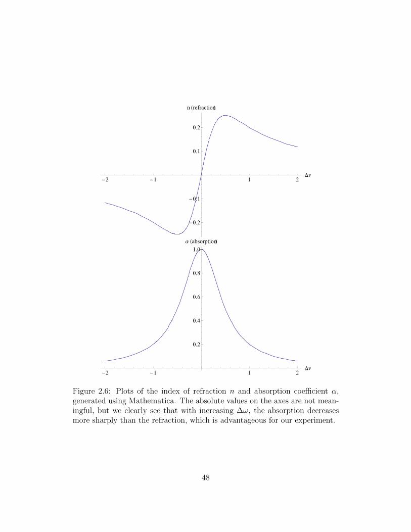
-2 -1 1 2DΝ
-0.2
-0.1
0.1
0.2
n HrefractionL
-2 -1 1 2DΝ
0.2
0.4
0.6
0.8
1.0
Α HabsorptionL
Figure 2.6: Plots of the index of refraction n and absorption coefficient α,generated using Mathematica. The absolute values on the axes are not mean-ingful, but we clearly see that with increasing ∆ν, the absorption decreasesmore sharply than the refraction, which is advantageous for our experiment.
47
Figure 2.6: Plots of the index of refraction n and absorption coefficient α,generated using Mathematica. The absolute values on the axes are not mean-ingful, but we clearly see that with increasing ∆ω, the absorption decreasesmore sharply than the refraction, which is advantageous for our experiment.
48
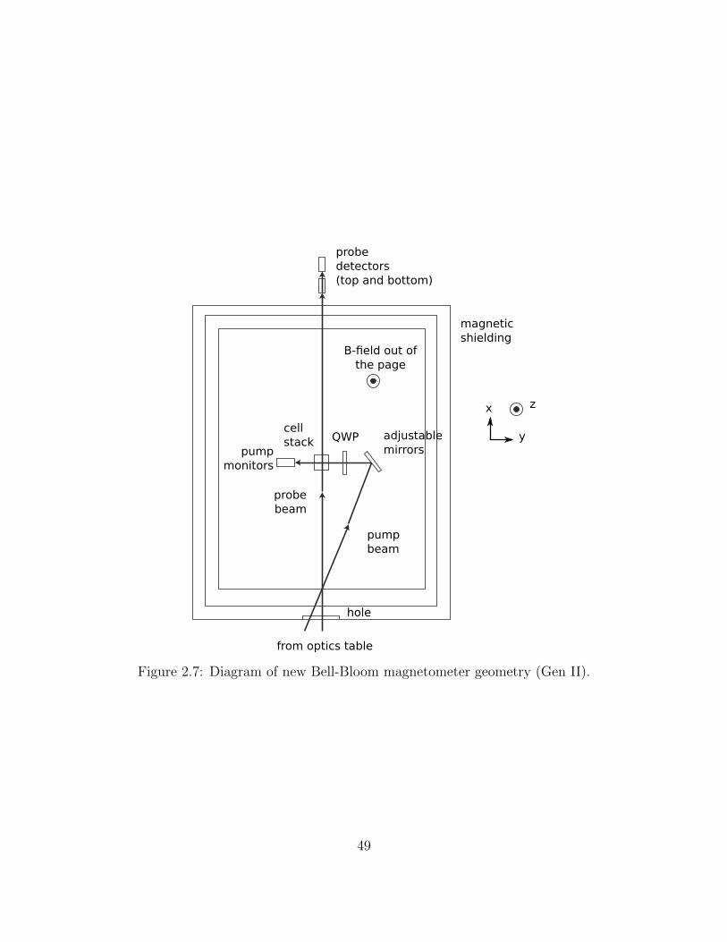
B-field out of the page
probedetectors(top and bottom)
QWP adjustablemirrorspump
monitors
cell stack
hole
from optics table
x
y
z
pumpbeam
probebeam
magneticshielding
Figure 2.7: Diagram of new Bell-Bloom magnetometer geometry (Gen II).
49
2.4 The Old Gen I Experiment
In this section, we will review basic features of the previous generation of our
magnetometer apparatus. Much work has been done by several previous stu-
dents on this experiment dating back to 2002 [63–66]; the most comprehensive
document is David Stein’s thesis [56]. Most of the details on the Gen I ap-
paratus have been thoroughly expounded in these theses, and so here we will
only recap the features as needed.
2.4.1 Searching for Local Lorentz Invariance
The Gen I optical magnetometer was used to search not for LRSSIs but for
violations of Local Lorentz Invariance (LLI). An LLI violation would constitute
a coupling between the spin of a particle to a direction in space, in the form
of
H = Ks · r, (2.47)
where r points along the preferred direction and K is a coupling constant.
Apart from this, the physics is similar to our current search for LRSSIs; after
obtaining the upper limit for the difference in Hg frequency between the two
table positions (∆vHgN ), instead of chugging it through the equations for various
LRSSI potentials, we would just use Eq. 2.47. The latest experimental results
for this experiment was published in [47]. Gen I was mainly concerned with
upper bounds for couplings to directions in the plane of the Earth’s rotation
(in other words, equatorial dipole couplings); this is the parameter b⊥. The
apparatus also had sensitivity to directional couplings along the Earth’s spin
50
axis bz. While Gen I initially had the best limits on b⊥, eventually other
experiments superseded it for couplings for the neutron and proton [43] as
well as the electron [67]. Gen I still had the best limits on bz, a somewhat less
attractive parameter as it only deals with couplings along a single line. With
the advent of the new geophysical method detailed in Chapter 1, however, the
apparatus has a newfound purpose as it turned out to be better than other
experiments for bounding LRSSIs for several regimes. This led to the project
of the present thesis.
2.4.2 The Mx-Geometry of Gen I
The optical geometry of Gen I is commonly termed the Mx geometry [61],
shown in Fig. 2.8. Unlike Gen II, this geometry uses a single beam to both
pump and probe the atoms, which in the figure is depicted as propagating
along the z-axis. As we used the same 62S1/2 → 62P1/2 transition for the Cs
cells,5 the laser was also circularly polarized and tuned to 894.4 nm, but it is
shining constantly instead of being modulated. For the Hg cells, ultraviolet
254 nm light was used to pump the 61S0(F = 12) → 63P1(F ′ = 1
2) transition.
A static magnetic field Bapp is directed at an angle θB from the z-axis. As the
lasers are constantly on, while the atoms will still be optically pumped, their
spins will not precess in phase. While there is still a net polarization along
B, the transverse polarization will be scrambled so there is no observable
precession. This is where the oscillating magnetic field Bosc comes into play,
directed along the y-axis. The field is oscillating at the Larmor frequency, and
5A small difference was that the hyperfine levels used were F = 4 to F ′ = 3.
51
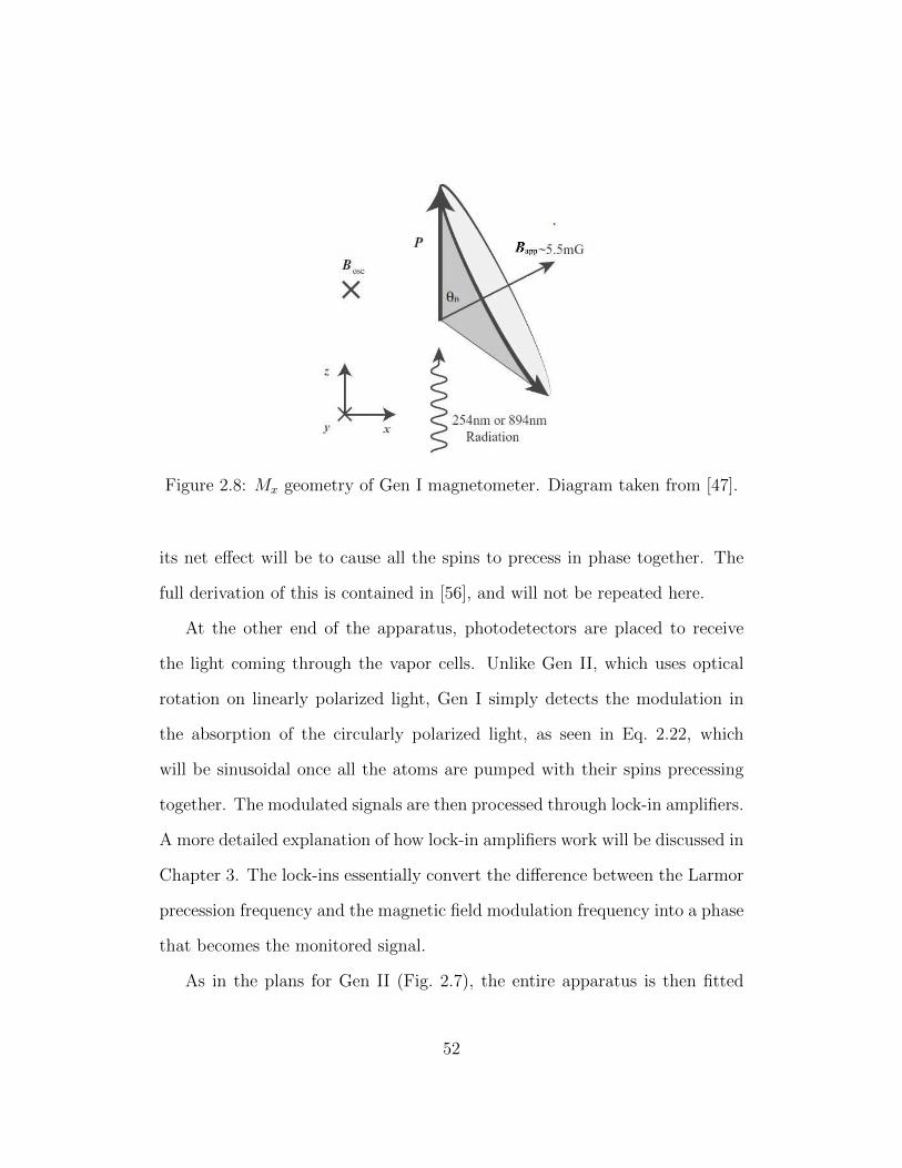
Figure 2.8: Mx geometry of Gen I magnetometer. Diagram taken from [47].
its net effect will be to cause all the spins to precess in phase together. The
full derivation of this is contained in [56], and will not be repeated here.
At the other end of the apparatus, photodetectors are placed to receive
the light coming through the vapor cells. Unlike Gen II, which uses optical
rotation on linearly polarized light, Gen I simply detects the modulation in
the absorption of the circularly polarized light, as seen in Eq. 2.22, which
will be sinusoidal once all the atoms are pumped with their spins precessing
together. The modulated signals are then processed through lock-in amplifiers.
A more detailed explanation of how lock-in amplifiers work will be discussed in
Chapter 3. The lock-ins essentially convert the difference between the Larmor
precession frequency and the magnetic field modulation frequency into a phase
that becomes the monitored signal.
As in the plans for Gen II (Fig. 2.7), the entire apparatus is then fitted
52
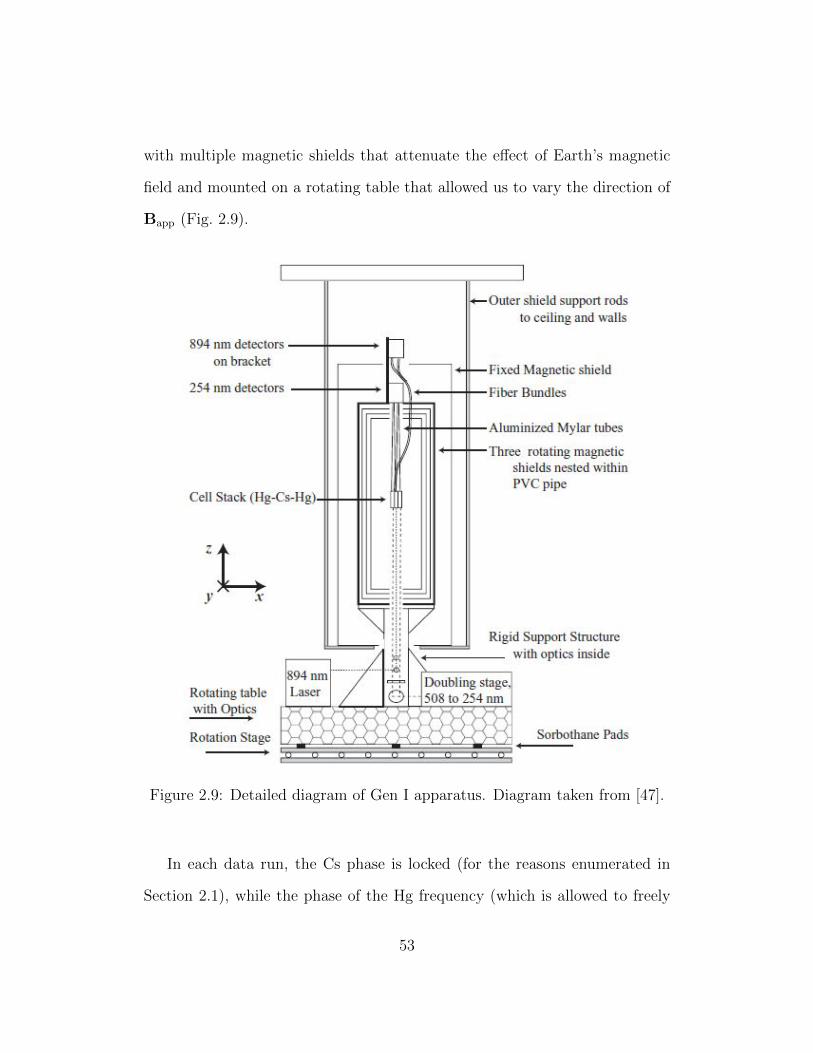
with multiple magnetic shields that attenuate the effect of Earth’s magnetic
field and mounted on a rotating table that allowed us to vary the direction of
Bapp (Fig. 2.9).
Figure 2.9: Detailed diagram of Gen I apparatus. Diagram taken from [47].
In each data run, the Cs phase is locked (for the reasons enumerated in
Section 2.1), while the phase of the Hg frequency (which is allowed to freely
53
vary) is monitored for a set amount of time (in this case, 124 seconds) with
the apparatus is in one table position. The table is then rotated into the other
position, and the phase is monitored for the same period of time. This process
was reiterated over about a week, and that constitutes one full data run.
A total of 12 data runs were needed to result in the bounds published in [47].
As the data was collected over multiple days, the apparatus did indeed detect
frequency shifts between the table positions, an average value of ∆νoffset =
15.75(5) µHz.
Most of this difference was due to the rotation frequency of the Earth,
which at a period of 23 hours, 56 minutes, and 4 seconds is 11.6 µHz. From a
combination of several factors such as the ratio of the gyromagnetic ratios of Hg
and Cs, a misalignment between the apparatus an true north, and also a small
effect by the Earth’s gyroscopic motion on the Cs oscillator, the apparatus was
calculated to have a sensitivity to the Earth’s gyroscopic frequency νpred =
15.39(2) µHz. Thus there remained a difference of ∆νg = 0.36(7) µHz, which
was thought probably not to have come as a result of LLI violations nor LRSSIs
but a systematic limitation of the Gen I apparatus, namely AC light shift. This
will be the subject of the next section.
2.5 AC Light Shift
Light shifts are shifts in the atomic energy levels that occur due to laser light.
Mathur et. al [68] identify the general light shift operator δE as consisting of
54
four terms:6
δE = δE0 + hδAI · J− µ · δH + δE2. (2.48)
The first term δE0 is called the center of mass light shift, and results in equal
displacement of all energy levels. As in optical pumping we are only con-
cerned about the differences between energy levels, it is not relevant to our
experiment. The second term, hδAI · J, is called the hyperfine structure light
shift and depends on the spectral profile of the light but not its polarization.
It does affect transitions with ∆F = 1, but it does not affect the magnetic
sub-levels mF . The third term, µ · δH, is a Zeeman light shift which occurs
when the light has some circular polarization, and it is the main form of light
shift that we are concerned about, and which we have been referring to as
AC light shift due to it arising from circularly polarized light. As stated in
Mathur’s paper, this light shift can be thought of as an additional magnetic
field H pointing parallel or anti-parallel to the direction of propagation of the
light and interacting with the atom to cause additional Zeeman shifts.
2.5.1 AC Light Shift in Gen I
In Gen I, the applied B-field (Bapp in Fig. 2.8) was at an angle θB = 63.8
from the propagation direction of the circularly polarized light beam. Thus
a significant component of the virtual B-field arising from the Zeeman light
shift affected the magnetic field experienced by the atoms. This can be seen
6The use of δ in front of each of these terms is a convention initially adapted by Happerand Mathur in their 1961 paper about operator formalism in discussions of optical pump-ing [69]. The δ is meant to differentiate physical effects coming from the laser light, asopposed to electric and magnetic fields that are deliberately applied through other means.
55
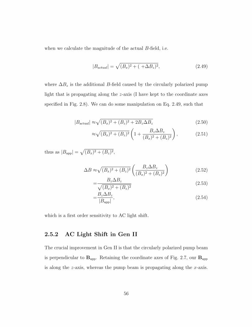
when we calculate the magnitude of the actual B-field, i.e.
|Bactual| =√
(Bx)2 + ( +∆Bz)2, (2.49)
where ∆Bz is the additional B-field caused by the circularly polarized pump
light that is propagating along the z-axis (I have kept to the coordinate axes
specified in Fig. 2.8). We can do some manipulation on Eq. 2.49, such that
|Bactual| ≈√
(Bx)2 + (Bz)2 + 2Bz∆Bz (2.50)
≈√
(Bx)2 + (Bz)2
(1 +
Bz∆Bz
(Bx)2 + (Bz)2
), (2.51)
thus as |Bapp| =√
(Bx)2 + (Bz)2,
∆B ≈√
(Bx)2 + (Bz)2
(Bz∆Bz
(Bx)2 + (Bz)2
)(2.52)
=Bz∆Bz√
(Bx)2 + (Bz)2(2.53)
=Bz∆Bz
|Bapp|, (2.54)
which is a first order sensitivity to AC light shift.
2.5.2 AC Light Shift in Gen II
The crucial improvement in Gen II is that the circularly polarized pump beam
is perpendicular to Bapp. Retaining the coordinate axes of Fig. 2.7, our Bapp
is along the z-axis, whereas the pump beam is propagating along the x-axis.
56
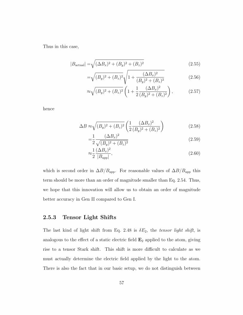
Thus in this case,
|Bactual| =√
(∆Bx)2 + (By)2 + (Bz)2 (2.55)
=√
(By)2 + (Bz)2
√1 +
(∆Bx)2
(By)2 + (Bz)2(2.56)
≈√
(By)2 + (Bz)2
(1 +
1
2
(∆Bx)2
(By)2 + (Bz)2
), (2.57)
hence
∆B ≈√
(By)2 + (Bz)2
(1
2
(∆Bx)2
(By)2 + (Bz)2
)(2.58)
=1
2
(∆Bx)2√
(By)2 + (Bz)2(2.59)
≈1
2
(∆Bx)2
|Bapp|, (2.60)
which is second order in ∆B/Bapp. For reasonable values of ∆B/Bapp this
term should be more than an order of magnitude smaller than Eq. 2.54. Thus,
we hope that this innovation will allow us to obtain an order of magnitude
better accuracy in Gen II compared to Gen I.
2.5.3 Tensor Light Shifts
The last kind of light shift from Eq. 2.48 is δE2, the tensor light shift, is
analogous to the effect of a static electric field E2 applied to the atom, giving
rise to a tensor Stark shift. This shift is more difficult to calculate as we
must actually determine the electric field applied by the light to the atom.
There is also the fact that in our basic setup, we do not distinguish between
57
magnetic sublevels. The shift ∆E for a Zeeman sublevel M is calculated to
be proportional to the Legendre polynomial P2 (Problem 2.11 of [70]), i.e.,
∆E(M) ∝ 3 cos2 θ − 1
2[3M2 − F (F + 1)], (2.61)
where θ is the angle between E2 to Bapp. Thus, when we set P2(θ) = 0, that
is, θ ≈ 54.7, we will minimize the effect of this light shift. We anticipate that
this effect will be smaller than the Zeeman light shift. At this time, we are
still experimentally investigating the extent of the latter, so the tensor light
shift will be a topic to be explored only in the future.
2.6 Two Pumping and Probing Schemes
In the process of implementing Gen II, there are two possible alternative pump-
ing and probing schemes that we are investigating. Both of these utilize the
same optical geometry of Fig. 2.7, but differ in the method of collecting data.
The main aim of this thesis is to explore both schemes and eventually de-
termine which one will be more advantageous for improving our bounds on
LRSSIs.
2.6.1 Scheme I: Pump then Probe (PTP)
In this scheme, the probe light is always on, and the photodetectors are con-
nected directly to the computer via the DAQ (Data Acquisition System). In
a single run, we turn on the modulated pump light for an amount of time
58
until the polarization is fully pumped, usually about 200 ms or so for our Cs
cells. The pump light is then turned off, and the atom will keep oscillating for
a while due to the Larmor precession of the atomic polarization, which is re-
flected in the oscillation of the probe light detected by the detectors. However,
the oscillation decays with a time constant T2. As has been mentioned before,
it is the difference channel (between the two orthogonal linear polarizations)
that we analyze. An example of a trace recorded by the DAQ for a single run
is shown in Fig. 2.10. During the portion from t = 0 to t = 200 ms, we see
an expanding signal, which indicates the atoms are gradually being pumped
into a coherent polarization. In this trace, the pumping is stopped at t = 200
ms as we found out that pumping longer does not further expand the signal,
indicating that this amount of time is about just enough to achieve a stable
state of polarization. For the next 400 ms, we let the signal decay and record
the oscillations. This portion of the trace is fitted in LabVIEW to a decaying
function in the form
y = A3e−t/A4 sin(A1t+ A2), (2.62)
where A1, the frequency of the modulation, is the main fit parameter that we
are concerned about.7 Note that A4 is equal to the lifetime T2. We repeat this
process over many runs, monitoring any changes in A1.
The main advantage of the PTP scheme is that the pump light is off when
the probing takes place. Thus in principle, we should not be too vulnerable
7We could have added an additional fit parameter A5 for a linear offset to Eq. 2.62, butLabVIEW was able to fit without specifying this parameter, so we omitted it.
59
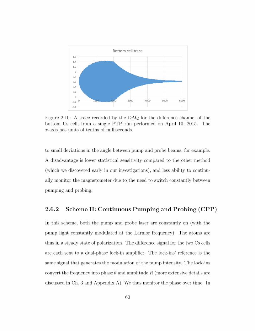
-0.4
-0.2
0
0.2
0.4
0.6
0.8
1
1.2
1.4
1.6
0 1000 2000 3000 4000 5000 6000
Bottom cell trace
Figure 2.10: A trace recorded by the DAQ for the difference channel of thebottom Cs cell, from a single PTP run performed on April 10, 2015. Thex-axis has units of tenths of milliseconds.
to small deviations in the angle between pump and probe beams, for example.
A disadvantage is lower statistical sensitivity compared to the other method
(which we discovered early in our investigations), and less ability to continu-
ally monitor the magnetometer due to the need to switch constantly between
pumping and probing.
2.6.2 Scheme II: Continuous Pumping and Probing (CPP)
In this scheme, both the pump and probe laser are constantly on (with the
pump light constantly modulated at the Larmor frequency). The atoms are
thus in a steady state of polarization. The difference signal for the two Cs cells
are each sent to a dual-phase lock-in amplifier. The lock-ins’ reference is the
same signal that generates the modulation of the pump intensity. The lock-ins
convert the frequency into phase θ and amplitude R (more extensive details are
discussed in Ch. 3 and Appendix A). We thus monitor the phase over time. In
60
order to convert changes in the phase to changes in the frequency (essentially,
finding out the value of dν/dθ), we do a test where we change the frequency
of the pump modulation by a small amount (0.5 Hz higher and lower in our
standard procedure) and see how much the phase changes from this artificial
tinkering. This allows us to calibrate the sensitivity of each cell.
The main advantage of the CPP scheme is that its statistics are much better
than PTP (in fact, about an order of magnitude better in our investigation, as
will be seen in Ch. 6). It also allows for more continuous, uniform monitoring
of the magnetometer’s B-field, and we will not encounter curve-fitting failures
like we sometimes do in the case of PTP, as we are just monitoring values
of the phase. The main disadvantage, however, is that we anticipate it to be
very sensitive to changes in the angle between the pump and probe lasers.
This is a serious concern, as in the actual experiment, the apparatus will be
rotated 180 every few minutes, and from our past experiences with the Gen I
apparatus, small shifts in the directions of the laser light are to be expected.
Thus, a major objective in the thesis is to see whether increased sensitivity to
systematics will outweigh the inherent statistical advantages of CPP.
2.7 Target Sensitivity
Before we delve into experimental investigation of the two schemes, it is crucial
to explicitly spell out the level of improvement we are hoping to achieve. At
the 1 sigma level, Gen I managed to achieve a sensitivity of
∆vHgN < 0.7 µHz. (2.63)
61
Our target is an order of magnitude better than this, i.e.
∆vHgN < 0.07 µHz. (2.64)
First, we consider the gyromagnetic ratios of Cs and Hg, which determine their
Larmor precession frequency. They are
γCs ≈ 350kHz/G (2.65)
γHg ≈ 759Hz/G, (2.66)
and because the magnetic field is locked to the Cs cells, while we are observing
the Hg cells, we are concerned with the ratio between the two gyromagnetic
ratios, i.e.
γCs
γHg
≈ 461. (2.67)
Thus, when we are working with only Cs cells, we will need to achieve a
sensitivity of
∆vCsN < 0.07× 461 = 32 µHz. (2.68)
Now the relation between the standard error SE, sample standard deviation σ
and number of data points N is
SE =σ√N. (2.69)
Assume that we would want to make a single measurement after about a week
(∼10, 000 min = 6×10⁵ s) of running data, and that tdata is the time in seconds
62

needed to take one data point. Thus we would want the standard deviation of
the Cs frequency, σνCsto be
σνCs< 32× 10−6 ×
√6× 10⁵
tdata(2.70)
Thus this is the target we are to keep in mind as we investigate both the
PTP and CPP schemes (which have different values of tdata) in the following
chapters.
2.8 Summary
In this chapter, we have fully described the physics behind our experimen-
tal apparatus that allow us to look for the spin-spin interactions described in
Ch. 1. We have seen how spin couples to magnetic fields, and how magnetic
fields cause Larmor precession in the atoms of the co-magnetometer, making
it possible to look for spin-spin interactions by monitoring their precession fre-
quency. We have explained how we monitor this frequency by optical pumping
and probing, and how our new optical geometry is projected to perform better
with regards to AC light shift, which was the limitation for Gen I. In the next
chapter, we shall describe more technical details about the equipment used to
perform the experiment described in this chapter.
63
Chapter 3
Experimental Apparatus
In this chapter we shall describe and discuss the various pieces of equipment
that make up our apparatus. We shall note any differences between Gen I and
Gen II along the way.
3.1 Rotating Table and the Test Table
We ultimately hope to be able to implement Gen II on a rotating table, as
with Gen I. A photo of the rotating-table apparatus is shown in Fig. 3.1.
There are many challenges, however, to working directly on the rotating table
apparatus, as the vertical layout requires one to climb a ladder in order to
take the cells in and out, and we would also have to find a way to mount the
photo-detectors on top of the cylindrical cans1. Attempting to surmount all
these physical challenges while also exploring a new optical geometry would
1In the rest of this chapter, “cans” refers to the cylindrical layers of magnetic shieldingthat encase the cells and the cell mounting.
64
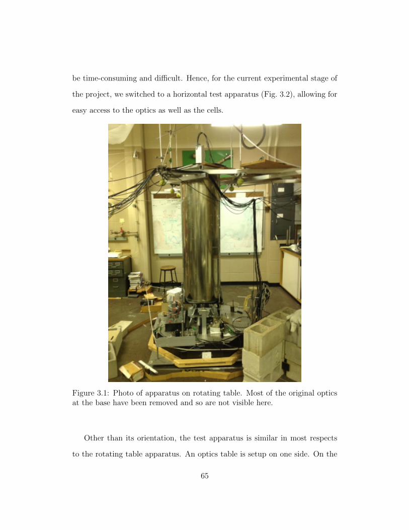
be time-consuming and difficult. Hence, for the current experimental stage of
the project, we switched to a horizontal test apparatus (Fig. 3.2), allowing for
easy access to the optics as well as the cells.
Figure 3.1: Photo of apparatus on rotating table. Most of the original opticsat the base have been removed and so are not visible here.
Other than its orientation, the test apparatus is similar in most respects
to the rotating table apparatus. An optics table is setup on one side. On the
65
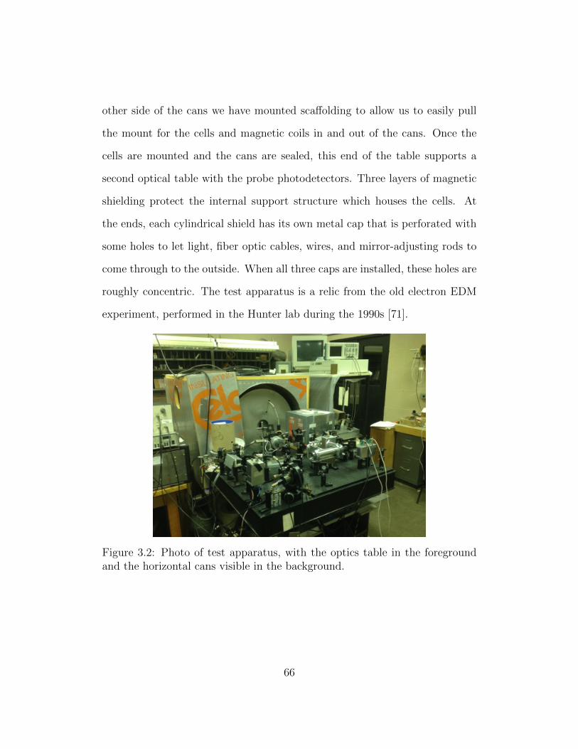
other side of the cans we have mounted scaffolding to allow us to easily pull
the mount for the cells and magnetic coils in and out of the cans. Once the
cells are mounted and the cans are sealed, this end of the table supports a
second optical table with the probe photodetectors. Three layers of magnetic
shielding protect the internal support structure which houses the cells. At
the ends, each cylindrical shield has its own metal cap that is perforated with
some holes to let light, fiber optic cables, wires, and mirror-adjusting rods to
come through to the outside. When all three caps are installed, these holes are
roughly concentric. The test apparatus is a relic from the old electron EDM
experiment, performed in the Hunter lab during the 1990s [71].
Figure 3.2: Photo of test apparatus, with the optics table in the foregroundand the horizontal cans visible in the background.
66
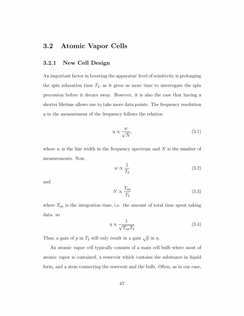
3.2 Atomic Vapor Cells
3.2.1 New Cell Design
An important factor in boosting the apparatus’ level of sensitivity is prolonging
the spin relaxation time T2, as it gives us more time to interrogate the spin
precession before it decays away. However, it is also the case that having a
shorter lifetime allows one to take more data points. The frequency resolution
η in the measurement of the frequency follows the relation
η ∝ w√N, (3.1)
where w is the line width in the frequency spectrum and N is the number of
measurements. Now,
w ∝ 1
T2
(3.2)
and
N ∝ Tint
T2
(3.3)
where Tint is the integration time, i.e. the amount of total time spent taking
data. so
η ∝ 1√TintT2
(3.4)
Thus, a gain of p in T2 will only result in a gain√p in η.
An atomic vapor cell typically consists of a main cell bulb where most of
atomic vapor is contained, a reservoir which contains the substance in liquid
form, and a stem connecting the reservoir and the bulb. Often, as in our case,
67
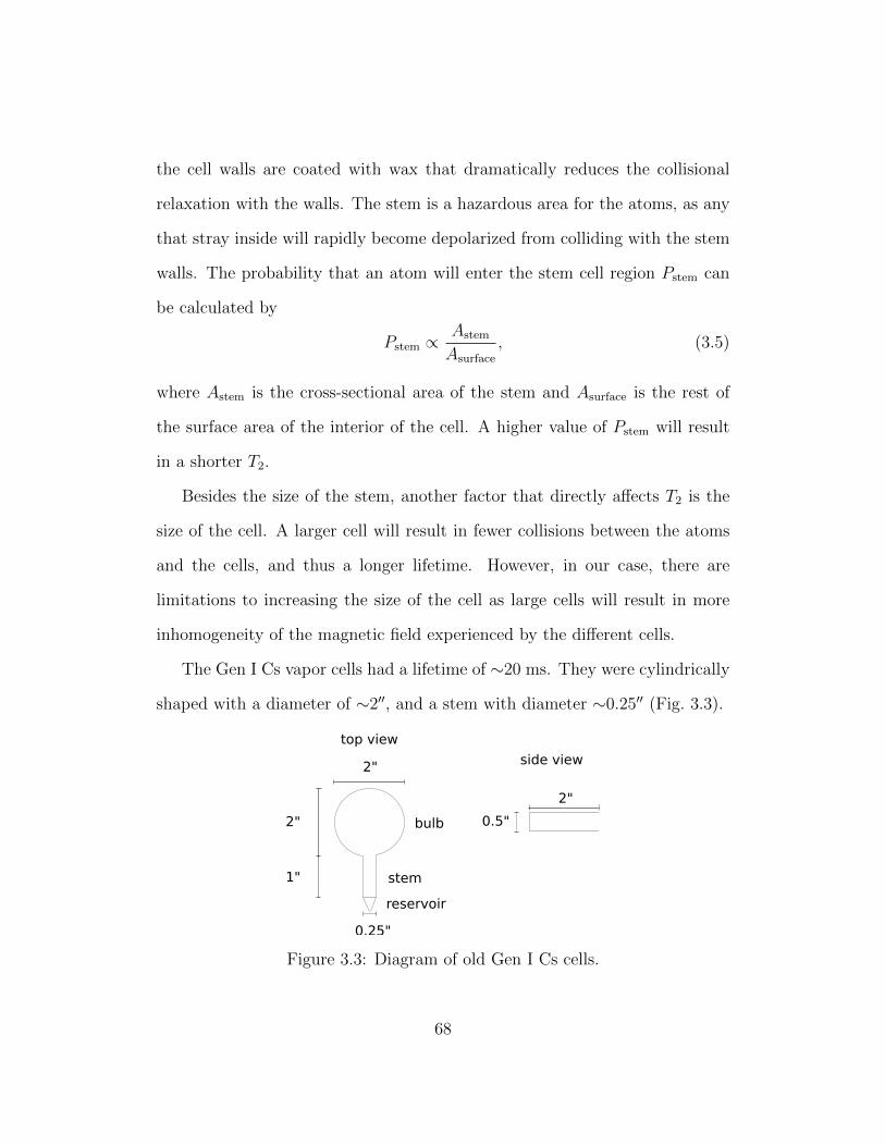
the cell walls are coated with wax that dramatically reduces the collisional
relaxation with the walls. The stem is a hazardous area for the atoms, as any
that stray inside will rapidly become depolarized from colliding with the stem
walls. The probability that an atom will enter the stem cell region Pstem can
be calculated by
Pstem ∝Astem
Asurface
, (3.5)
where Astem is the cross-sectional area of the stem and Asurface is the rest of
the surface area of the interior of the cell. A higher value of Pstem will result
in a shorter T2.
Besides the size of the stem, another factor that directly affects T2 is the
size of the cell. A larger cell will result in fewer collisions between the atoms
and the cells, and thus a longer lifetime. However, in our case, there are
limitations to increasing the size of the cell as large cells will result in more
inhomogeneity of the magnetic field experienced by the different cells.
The Gen I Cs vapor cells had a lifetime of ∼20 ms. They were cylindrically
shaped with a diameter of ∼2′′, and a stem with diameter ∼0.25′′ (Fig. 3.3).
2"
1"
0.5"
top view
side view2"
0.25"
2"
stem
reservoir
bulb
Figure 3.3: Diagram of old Gen I Cs cells.
68
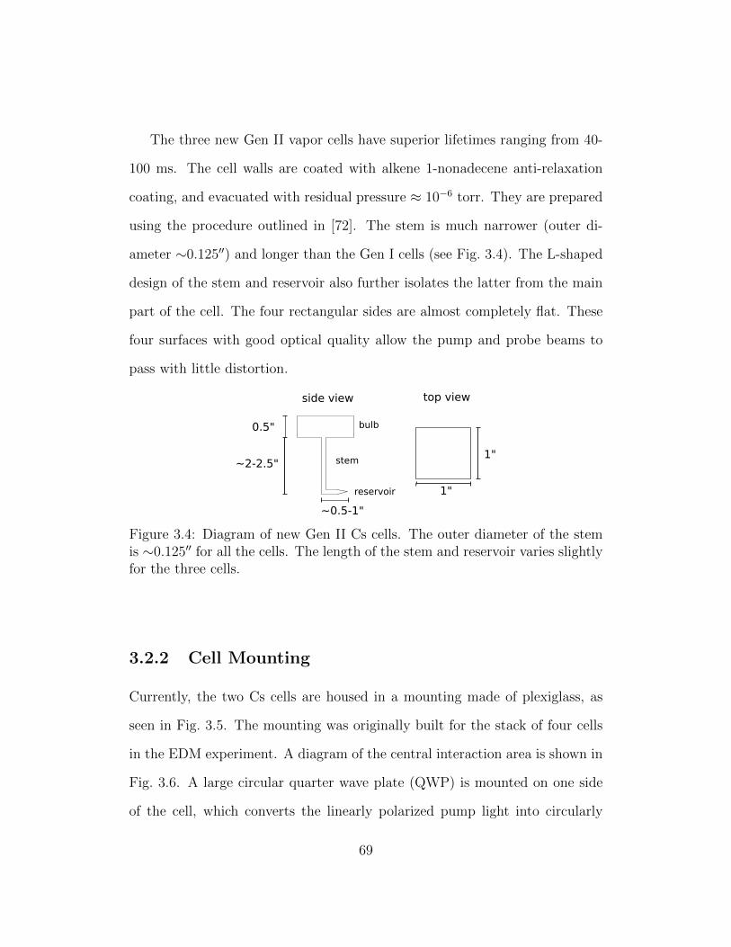
The three new Gen II vapor cells have superior lifetimes ranging from 40-
100 ms. The cell walls are coated with alkene 1-nonadecene anti-relaxation
coating, and evacuated with residual pressure ≈ 10−6 torr. They are prepared
using the procedure outlined in [72]. The stem is much narrower (outer di-
ameter ∼0.125′′) and longer than the Gen I cells (see Fig. 3.4). The L-shaped
design of the stem and reservoir also further isolates the latter from the main
part of the cell. The four rectangular sides are almost completely flat. These
four surfaces with good optical quality allow the pump and probe beams to
pass with little distortion.
1"
1"
0.5"
~2-2.5"
~0.5-1"
stem
reservoir
bulb
side view top view
Figure 3.4: Diagram of new Gen II Cs cells. The outer diameter of the stemis ∼0.125′′ for all the cells. The length of the stem and reservoir varies slightlyfor the three cells.
3.2.2 Cell Mounting
Currently, the two Cs cells are housed in a mounting made of plexiglass, as
seen in Fig. 3.5. The mounting was originally built for the stack of four cells
in the EDM experiment. A diagram of the central interaction area is shown in
Fig. 3.6. A large circular quarter wave plate (QWP) is mounted on one side
of the cell, which converts the linearly polarized pump light into circularly
69
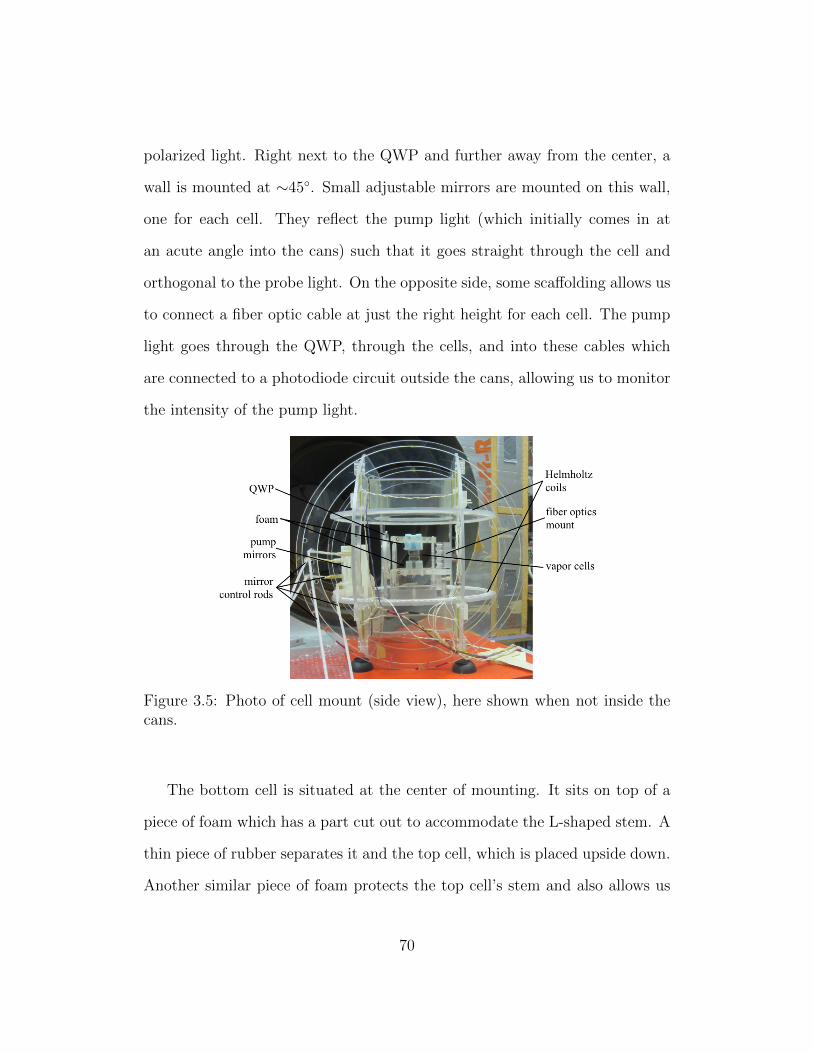
polarized light. Right next to the QWP and further away from the center, a
wall is mounted at ∼45. Small adjustable mirrors are mounted on this wall,
one for each cell. They reflect the pump light (which initially comes in at
an acute angle into the cans) such that it goes straight through the cell and
orthogonal to the probe light. On the opposite side, some scaffolding allows us
to connect a fiber optic cable at just the right height for each cell. The pump
light goes through the QWP, through the cells, and into these cables which
are connected to a photodiode circuit outside the cans, allowing us to monitor
the intensity of the pump light.
Figure 3.5: Photo of cell mount (side view), here shown when not inside thecans.
The bottom cell is situated at the center of mounting. It sits on top of a
piece of foam which has a part cut out to accommodate the L-shaped stem. A
thin piece of rubber separates it and the top cell, which is placed upside down.
Another similar piece of foam protects the top cell’s stem and also allows us
70
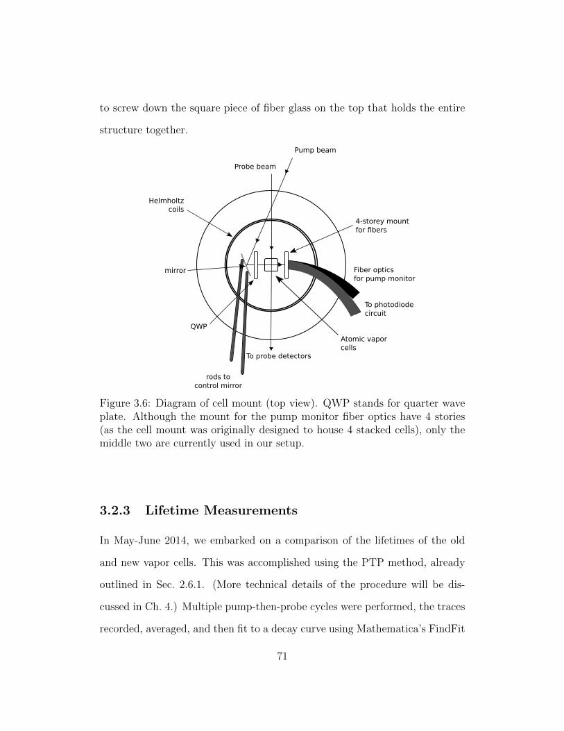
to screw down the square piece of fiber glass on the top that holds the entire
structure together.
QWP
Fiber opticsfor pump monitor
mirror
4-storey mountfor fibers
Probe beam
Pump beam
Helmholtzcoils
To probe detectors
Atomic vaporcells
rods tocontrol mirror
To photodiodecircuit
Figure 3.6: Diagram of cell mount (top view). QWP stands for quarter waveplate. Although the mount for the pump monitor fiber optics have 4 stories(as the cell mount was originally designed to house 4 stacked cells), only themiddle two are currently used in our setup.
3.2.3 Lifetime Measurements
In May-June 2014, we embarked on a comparison of the lifetimes of the old
and new vapor cells. This was accomplished using the PTP method, already
outlined in Sec. 2.6.1. (More technical details of the procedure will be dis-
cussed in Ch. 4.) Multiple pump-then-probe cycles were performed, the traces
recorded, averaged, and then fit to a decay curve using Mathematica’s FindFit
71
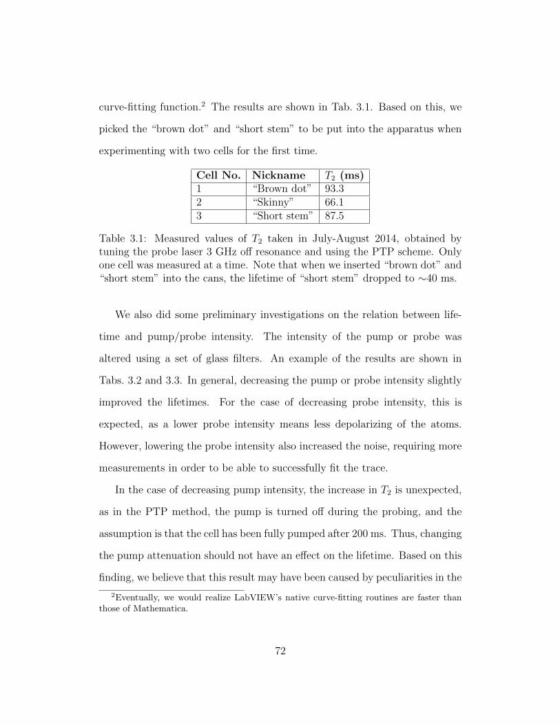
curve-fitting function.2 The results are shown in Tab. 3.1. Based on this, we
picked the “brown dot” and “short stem” to be put into the apparatus when
experimenting with two cells for the first time.
Cell No. Nickname T2 (ms)1 “Brown dot” 93.32 “Skinny” 66.13 “Short stem” 87.5
Table 3.1: Measured values of T2 taken in July-August 2014, obtained bytuning the probe laser 3 GHz off resonance and using the PTP scheme. Onlyone cell was measured at a time. Note that when we inserted “brown dot” and“short stem” into the cans, the lifetime of “short stem” dropped to ∼40 ms.
We also did some preliminary investigations on the relation between life-
time and pump/probe intensity. The intensity of the pump or probe was
altered using a set of glass filters. An example of the results are shown in
Tabs. 3.2 and 3.3. In general, decreasing the pump or probe intensity slightly
improved the lifetimes. For the case of decreasing probe intensity, this is
expected, as a lower probe intensity means less depolarizing of the atoms.
However, lowering the probe intensity also increased the noise, requiring more
measurements in order to be able to successfully fit the trace.
In the case of decreasing pump intensity, the increase in T2 is unexpected,
as in the PTP method, the pump is turned off during the probing, and the
assumption is that the cell has been fully pumped after 200 ms. Thus, changing
the pump attenuation should not have an effect on the lifetime. Based on this
finding, we believe that this result may have been caused by peculiarities in the
2Eventually, we would realize LabVIEW’s native curve-fitting routines are faster thanthose of Mathematica.
72
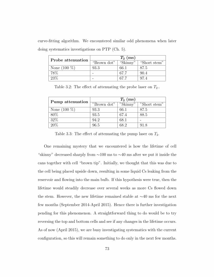
curve-fitting algorithm. We encountered similar odd phenomena when later
doing systematics investigations on PTP (Ch. 5).
Probe attenuationT2 (ms)
“Brown dot” “Skinny” “Short stem”None (100 %) 93.3 66.1 87.578% - 67.7 90.423% - 67.7 97.4
Table 3.2: The effect of attenuating the probe laser on T2..
Pump attenuationT2 (ms)
”Brown dot” ”Skinny” ”Short stem”None (100 %) 93.3 66.1 87.580% 93.5 67.4 88.532% 94.2 68.1 -20% 96.5 68.2 91.8
Table 3.3: The effect of attenuating the pump laser on T2.
One remaining mystery that we encountered is how the lifetime of cell
“skinny” decreased sharply from ∼100 ms to ∼40 ms after we put it inside the
cans together with cell “brown tip”. Initially, we thought that this was due to
the cell being placed upside down, resulting in some liquid Cs leaking from the
reservoir and flowing into the main bulb. If this hypothesis were true, then the
lifetime would steadily decrease over several weeks as more Cs flowed down
the stem. However, the new lifetime remained stable at ∼40 ms for the next
few months (September 2014-April 2015). Hence there is further investigation
pending for this phenomenon. A straightforward thing to do would be to try
reversing the top and bottom cells and see if any changes in the lifetime occurs.
As of now (April 2015), we are busy investigating systematics with the current
configuration, so this will remain something to do only in the next few months.
73
3.3 Magnetic Field Coils
3.3.1 Helmholtz Coils
Three pairs of Helmholtz coils, one for each dimension, encircle the cell mount-
ing structure inside the cans. Each pair contains 2× 10 turns of copper wire.
Currently only one pair is used as we are not yet locking the B-field to the
Cs frequency. This is the pair with the coils in the xy-plane, creating a ho-
mogeneous B-field in the z-direction. Thus, our z-axis is orthogonal to the
plane of the floor of the laboratory. For this pair, the upper set of turns are
spaced ∼6′′ from the bottom set. The upper and bottom sets are connected
in series, and the two ends of the cable are connected to a circuit that allows
both coarse and fine B-field control.
3.3.2 Fine Magnetic Field Control
The voltage across the external power supply can be modified by turning
a knob, but for practical purposes we always keep it set to a base voltage
Vbase = 9.74 V. It is connected to a simple circuit that allows us to finely
control the B-field (Fig. 3.7). We set Rbase = 1 kΩ and Rfine = 100 kΩ. When
we apply a voltage Vfine of several volts, as Rfine Rbase, a small amount of
additional current will be added to the current from Vbase, slightly increasing
the B-field.
Initially, we connected Vfine directly to either a DAQ output or to an auxil-
iary voltage output on one of our SRS dual-phase lock-in amplifiers. However,
when we were taking data using CPP, we found that the level of magnetic
74
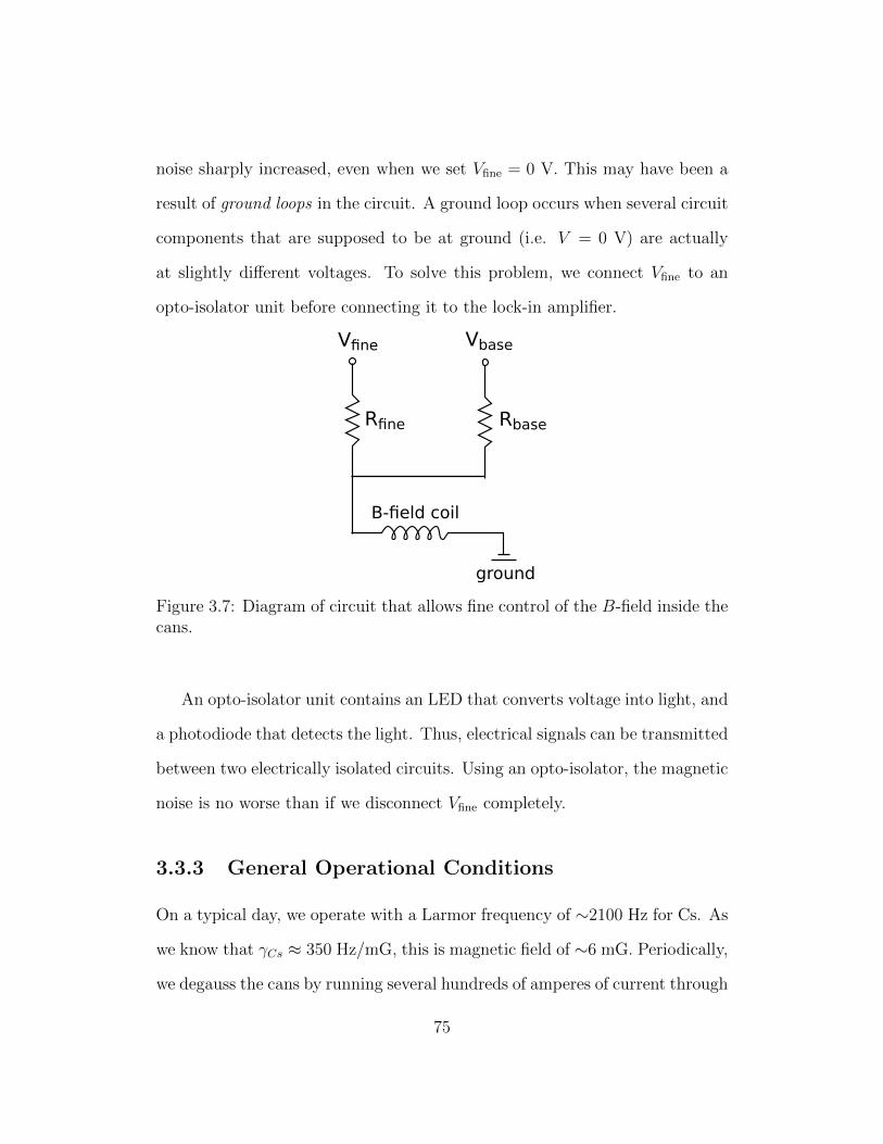
noise sharply increased, even when we set Vfine = 0 V. This may have been a
result of ground loops in the circuit. A ground loop occurs when several circuit
components that are supposed to be at ground (i.e. V = 0 V) are actually
at slightly different voltages. To solve this problem, we connect Vfine to an
opto-isolator unit before connecting it to the lock-in amplifier.
Rfine Rbase
B-field coil
Vfine Vbase
ground
Figure 3.7: Diagram of circuit that allows fine control of the B-field inside thecans.
An opto-isolator unit contains an LED that converts voltage into light, and
a photodiode that detects the light. Thus, electrical signals can be transmitted
between two electrically isolated circuits. Using an opto-isolator, the magnetic
noise is no worse than if we disconnect Vfine completely.
3.3.3 General Operational Conditions
On a typical day, we operate with a Larmor frequency of ∼2100 Hz for Cs. As
we know that γCs ≈ 350 Hz/mG, this is magnetic field of ∼6 mG. Periodically,
we degauss the cans by running several hundreds of amperes of current through
75
an annealing copper wire that goes through the cans. This is usually done after
we have fixed or tampered with the cell mounting, and results in small changes
of tens of Hz in the Larmor frequency.
3.4 Lasers
We shall now discuss the lasers that are used to pump and probe the atomic
vapor cells, including features that allow thermal stabilization and frequency
locking. For the case of Cs, Gen II uses the same type of lasers as Gen I, and
thus we will not discuss the Cs lasers in too much detail, as a more complete
treatment is available in Stein’s thesis [56]. Most of the discussion here is
based on this reference.
3.4.1 Cesium Laser System
Two separate external cavity diode lasers (ECDL) are used for pumping and
probing the Cs cells. Both lasers work in exactly the same way. Laser light
is produced by placing a Thor Labs LP880-SF3 (rated at 3 mW) laser diode
inside a cavity with a diffraction grating (Fig. 3.8). The diffraction grating
is attached to a piezoelectric chip that allows us to finely modify the length
of the cavity by applying a voltage to it. It is configured such that the first
order diffraction is reflected back in the cavity, providing optical feedback. The
zeroth order diffraction is deflected out of the cavity and becomes the output
76
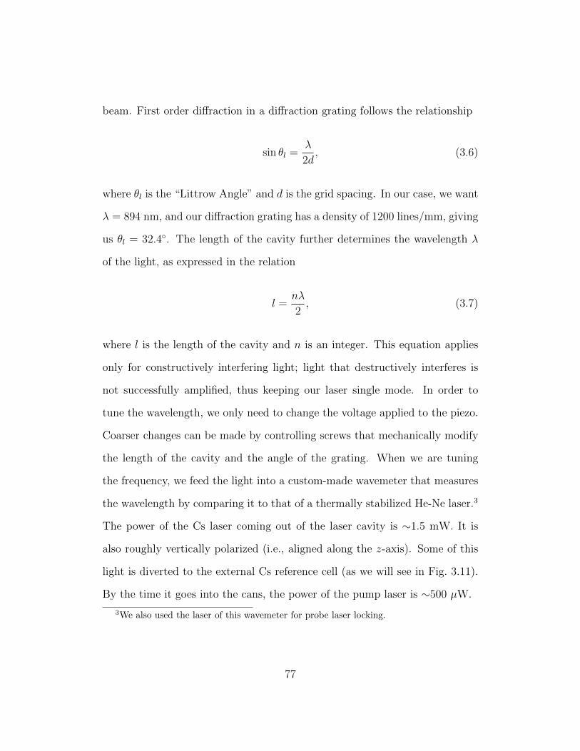
beam. First order diffraction in a diffraction grating follows the relationship
sin θl =λ
2d, (3.6)
where θl is the “Littrow Angle” and d is the grid spacing. In our case, we want
λ = 894 nm, and our diffraction grating has a density of 1200 lines/mm, giving
us θl = 32.4. The length of the cavity further determines the wavelength λ
of the light, as expressed in the relation
l =nλ
2, (3.7)
where l is the length of the cavity and n is an integer. This equation applies
only for constructively interfering light; light that destructively interferes is
not successfully amplified, thus keeping our laser single mode. In order to
tune the wavelength, we only need to change the voltage applied to the piezo.
Coarser changes can be made by controlling screws that mechanically modify
the length of the cavity and the angle of the grating. When we are tuning
the frequency, we feed the light into a custom-made wavemeter that measures
the wavelength by comparing it to that of a thermally stabilized He-Ne laser.3
The power of the Cs laser coming out of the laser cavity is ∼1.5 mW. It is
also roughly vertically polarized (i.e., aligned along the z-axis). Some of this
light is diverted to the external Cs reference cell (as we will see in Fig. 3.11).
By the time it goes into the cans, the power of the pump laser is ∼500 µW.
3We also used the laser of this wavemeter for probe laser locking.
77
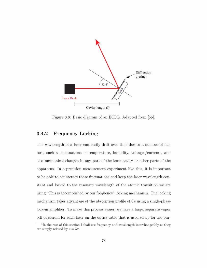
Figure 3.8: Basic diagram of an ECDL. Adapted from [56].
3.4.2 Frequency Locking
The wavelength of a laser can easily drift over time due to a number of fac-
tors, such as fluctuations in temperature, humidity, voltages/currents, and
also mechanical changes in any part of the laser cavity or other parts of the
apparatus. In a precision measurement experiment like this, it is important
to be able to counteract these fluctuations and keep the laser wavelength con-
stant and locked to the resonant wavelength of the atomic transition we are
using. This is accomplished by our frequency4 locking mechanism. The locking
mechanism takes advantage of the absorption profile of Cs using a single-phase
lock-in amplifier. To make this process easier, we have a large, separate vapor
cell of cesium for each laser on the optics table that is used solely for the pur-
4In the rest of this section I shall use frequency and wavelength interchangeably as theyare simply related by c = λν.
78
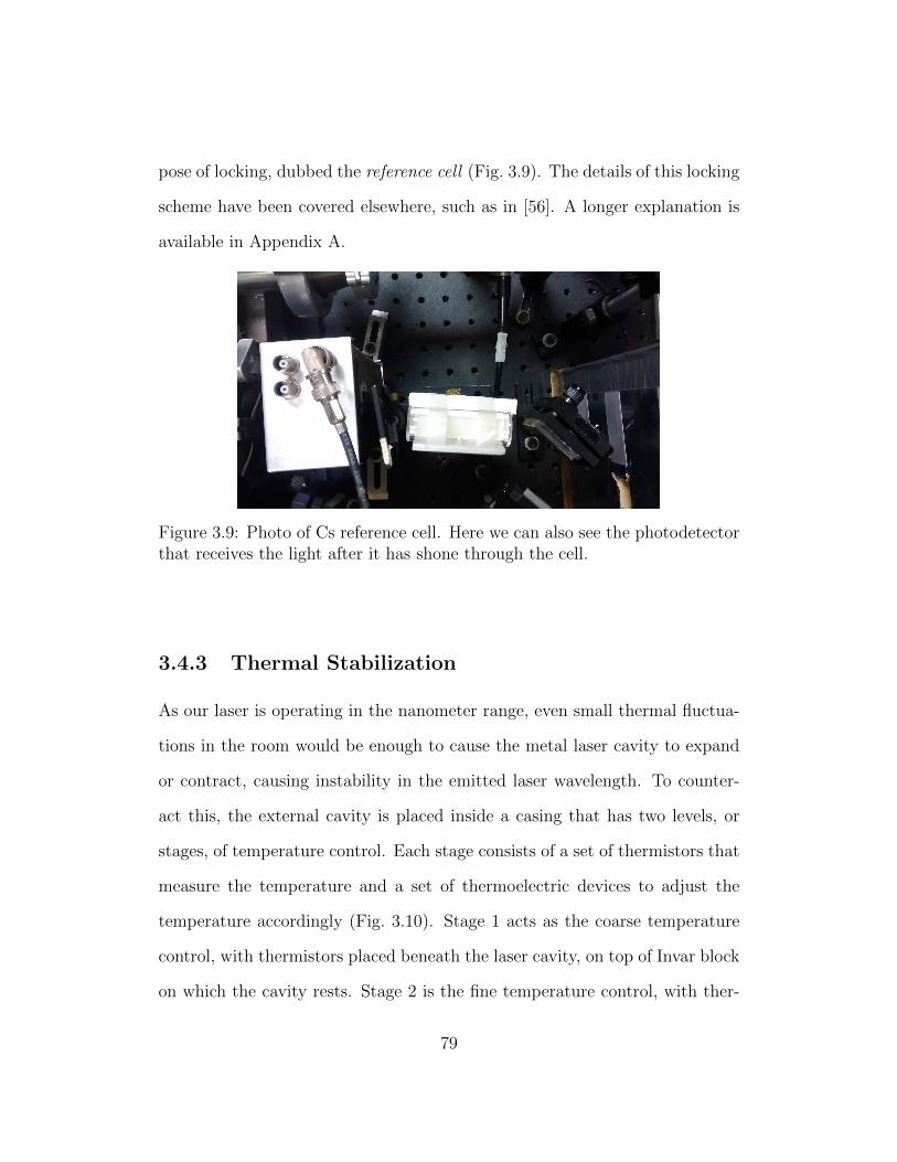
pose of locking, dubbed the reference cell (Fig. 3.9). The details of this locking
scheme have been covered elsewhere, such as in [56]. A longer explanation is
available in Appendix A.
Figure 3.9: Photo of Cs reference cell. Here we can also see the photodetectorthat receives the light after it has shone through the cell.
3.4.3 Thermal Stabilization
As our laser is operating in the nanometer range, even small thermal fluctua-
tions in the room would be enough to cause the metal laser cavity to expand
or contract, causing instability in the emitted laser wavelength. To counter-
act this, the external cavity is placed inside a casing that has two levels, or
stages, of temperature control. Each stage consists of a set of thermistors that
measure the temperature and a set of thermoelectric devices to adjust the
temperature accordingly (Fig. 3.10). Stage 1 acts as the coarse temperature
control, with thermistors placed beneath the laser cavity, on top of Invar block
on which the cavity rests. Stage 2 is the fine temperature control, with ther-
79
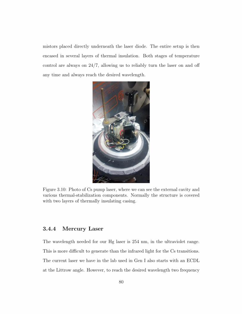
mistors placed directly underneath the laser diode. The entire setup is then
encased in several layers of thermal insulation. Both stages of temperature
control are always on 24/7, allowing us to reliably turn the laser on and off
any time and always reach the desired wavelength.
Figure 3.10: Photo of Cs pump laser, where we can see the external cavity andvarious thermal-stabilization components. Normally the structure is coveredwith two layers of thermally insulating casing.
3.4.4 Mercury Laser
The wavelength needed for our Hg laser is 254 nm, in the ultraviolet range.
This is more difficult to generate than the infrared light for the Cs transitions.
The current laser we have in the lab used in Gen I also starts with an ECDL
at the Littrow angle. However, to reach the desired wavelength two frequency
80
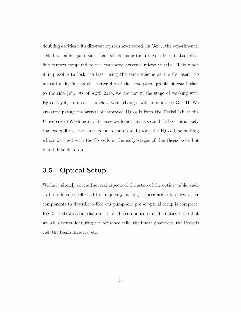
doubling cavities with different crystals are needed. In Gen I, the experimental
cells had buffer gas inside them which made them have different absorption
line centers compared to the evacuated external reference cells. This made
it impossible to lock the laser using the same scheme as the Cs laser. So
instead of locking to the center dip of the absorption profile, it was locked
to the side [56]. As of April 2015, we are not in the stage of working with
Hg cells yet, so it is still unclear what changes will be made for Gen II. We
are anticipating the arrival of improved Hg cells from the Heckel lab at the
University of Washington. Because we do not have a second Hg laser, it is likely
that we will use the same beam to pump and probe the Hg cell, something
which we tried with the Cs cells in the early stages of this thesis work but
found difficult to do.
3.5 Optical Setup
We have already covered several aspects of the setup of the optical table, such
as the reference cell used for frequency locking. There are only a few other
components to describe before our pump and probe optical setup is complete.
Fig. 3.11 shows a full diagram of all the components on the optics table that
we will discuss, featuring the reference cells, the linear polarizers, the Pockels
cell, the beam dividers, etc.
81
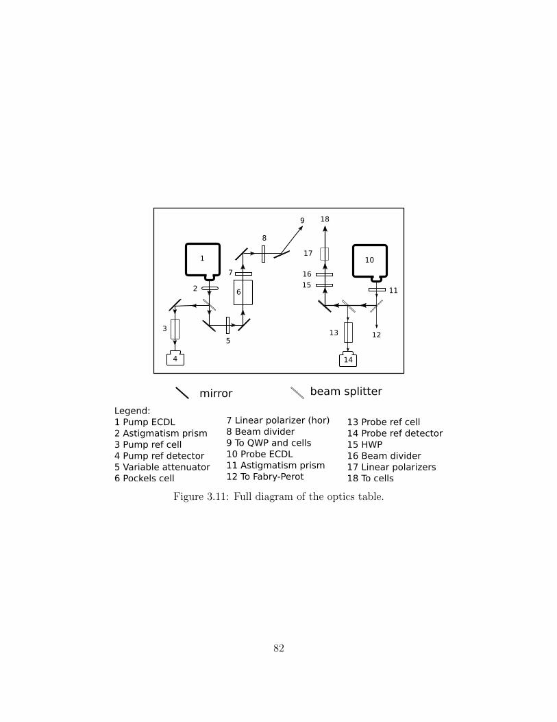
Legend:1 Pump ECDL2 Astigmatism prism3 Pump ref cell4 Pump ref detector5 Variable attenuator6 Pockels cell
7 Linear polarizer (hor)8 Beam divider9 To QWP and cells10 Probe ECDL11 Astigmatism prism12 To Fabry-Perot
13 Probe ref cell14 Probe ref detector15 HWP16 Beam divider17 Linear polarizers18 To cells
mirror beam splitter
1
2
3
4
5
6
7
8
9
10
11
1213
14
15
16
17
18
Figure 3.11: Full diagram of the optics table.
82
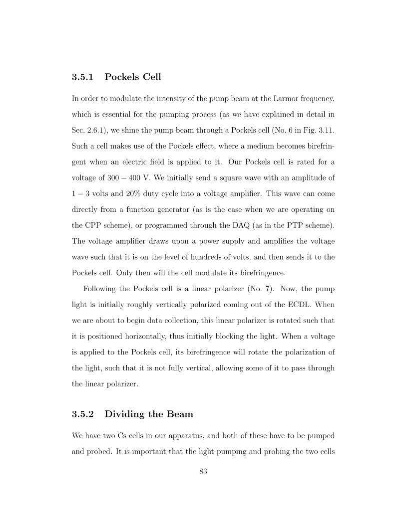
3.5.1 Pockels Cell
In order to modulate the intensity of the pump beam at the Larmor frequency,
which is essential for the pumping process (as we have explained in detail in
Sec. 2.6.1), we shine the pump beam through a Pockels cell (No. 6 in Fig. 3.11.
Such a cell makes use of the Pockels effect, where a medium becomes birefrin-
gent when an electric field is applied to it. Our Pockels cell is rated for a
voltage of 300− 400 V. We initially send a square wave with an amplitude of
1 − 3 volts and 20% duty cycle into a voltage amplifier. This wave can come
directly from a function generator (as is the case when we are operating on
the CPP scheme), or programmed through the DAQ (as in the PTP scheme).
The voltage amplifier draws upon a power supply and amplifies the voltage
wave such that it is on the level of hundreds of volts, and then sends it to the
Pockels cell. Only then will the cell modulate its birefringence.
Following the Pockels cell is a linear polarizer (No. 7). Now, the pump
light is initially roughly vertically polarized coming out of the ECDL. When
we are about to begin data collection, this linear polarizer is rotated such that
it is positioned horizontally, thus initially blocking the light. When a voltage
is applied to the Pockels cell, its birefringence will rotate the polarization of
the light, such that it is not fully vertical, allowing some of it to pass through
the linear polarizer.
3.5.2 Dividing the Beam
We have two Cs cells in our apparatus, and both of these have to be pumped
and probed. It is important that the light pumping and probing the two cells
83
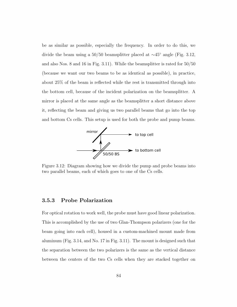
be as similar as possible, especially the frequency. In order to do this, we
divide the beam using a 50/50 beamsplitter placed at ∼45 angle (Fig. 3.12,
and also Nos. 8 and 16 in Fig. 3.11). While the beamsplitter is rated for 50/50
(because we want our two beams to be as identical as possible), in practice,
about 25% of the beam is reflected while the rest is transmitted through into
the bottom cell, because of the incident polarization on the beamsplitter. A
mirror is placed at the same angle as the beamsplitter a short distance above
it, reflecting the beam and giving us two parallel beams that go into the top
and bottom Cs cells. This setup is used for both the probe and pump beams.
to top cell
to bottom cell
mirror
50/50 BS
Figure 3.12: Diagram showing how we divide the pump and probe beams intotwo parallel beams, each of which goes to one of the Cs cells.
3.5.3 Probe Polarization
For optical rotation to work well, the probe must have good linear polarization.
This is accomplished by the use of two Glan-Thompson polarizers (one for the
beam going into each cell), housed in a custom-machined mount made from
aluminum (Fig. 3.14, and No. 17 in Fig. 3.11). The mount is designed such that
the separation between the two polarizers is the same as the vertical distance
between the centers of the two Cs cells when they are stacked together on
84
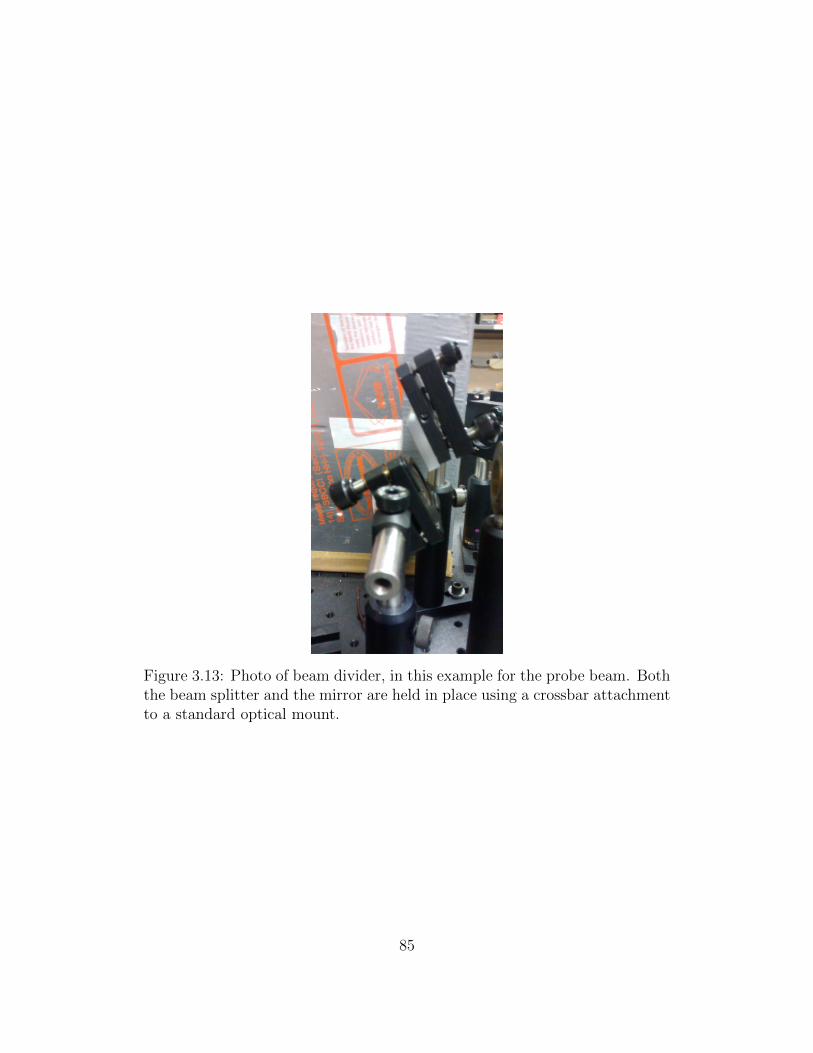
Figure 3.13: Photo of beam divider, in this example for the probe beam. Boththe beam splitter and the mirror are held in place using a crossbar attachmentto a standard optical mount.
85
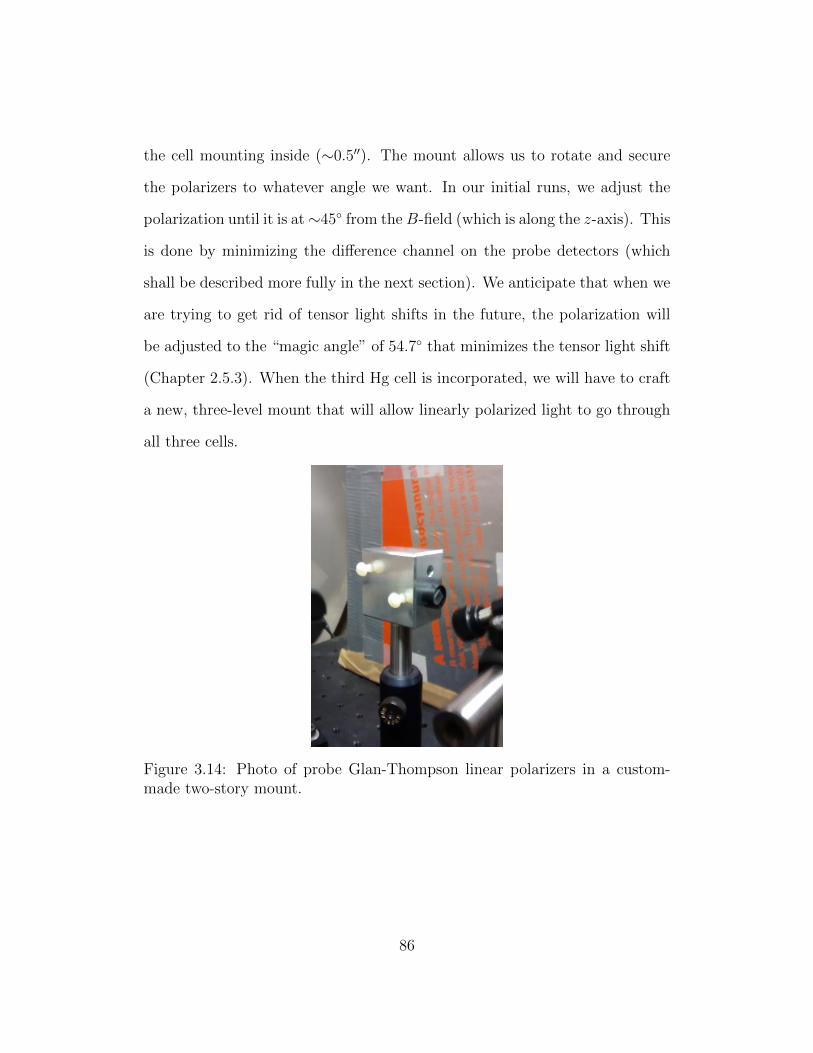
the cell mounting inside (∼0.5′′). The mount allows us to rotate and secure
the polarizers to whatever angle we want. In our initial runs, we adjust the
polarization until it is at∼45 from theB-field (which is along the z-axis). This
is done by minimizing the difference channel on the probe detectors (which
shall be described more fully in the next section). We anticipate that when we
are trying to get rid of tensor light shifts in the future, the polarization will
be adjusted to the “magic angle” of 54.7 that minimizes the tensor light shift
(Chapter 2.5.3). When the third Hg cell is incorporated, we will have to craft
a new, three-level mount that will allow linearly polarized light to go through
all three cells.
Figure 3.14: Photo of probe Glan-Thompson linear polarizers in a custom-made two-story mount.
86
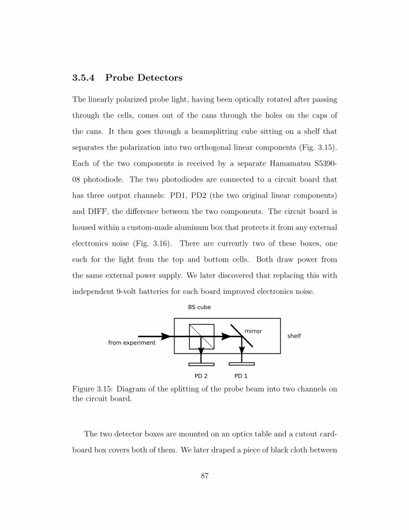
3.5.4 Probe Detectors
The linearly polarized probe light, having been optically rotated after passing
through the cells, comes out of the cans through the holes on the caps of
the cans. It then goes through a beamsplitting cube sitting on a shelf that
separates the polarization into two orthogonal linear components (Fig. 3.15).
Each of the two components is received by a separate Hamamatsu S5390-
08 photodiode. The two photodiodes are connected to a circuit board that
has three output channels: PD1, PD2 (the two original linear components)
and DIFF, the difference between the two components. The circuit board is
housed within a custom-made aluminum box that protects it from any external
electronics noise (Fig. 3.16). There are currently two of these boxes, one
each for the light from the top and bottom cells. Both draw power from
the same external power supply. We later discovered that replacing this with
independent 9-volt batteries for each board improved electronics noise.
PD 1PD 2
BS cube
mirror
from experimentshelf
Figure 3.15: Diagram of the splitting of the probe beam into two channels onthe circuit board.
The two detector boxes are mounted on an optics table and a cutout card-
board box covers both of them. We later draped a piece of black cloth between
87
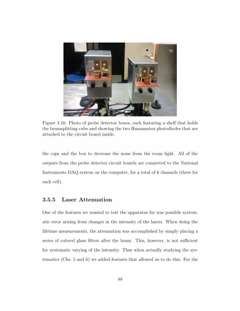
Figure 3.16: Photo of probe detector boxes, each featuring a shelf that holdsthe beamsplitting cube and showing the two Hamamatsu photodiodes that areattached to the circuit board inside.
the caps and the box to decrease the noise from the room light. All of the
outputs from the probe detector circuit boards are connected to the National
Instruments DAQ system on the computer, for a total of 6 channels (three for
each cell).
3.5.5 Laser Attenuation
One of the features we wanted to test the apparatus for was possible system-
atic error arising from changes in the intensity of the lasers. When doing the
lifetime measurements, the attenuation was accomplished by simply placing a
series of colored glass filters after the beam. This, however, is not sufficient
for systematic varying of the intensity. Thus when actually studying the sys-
tematics (Chs. 5 and 6) we added features that allowed us to do this. For the
88
pump, we put a variable attenuator that had a wheel with graduated levels of
aluminum on it. One increased or decreased the attenuation by spinning the
wheel. This is placed after the Pockels cell and the linear polarizer and right
before the light is divided into two.
Earlier, we had experimented with varying the intensity by adding addi-
tional optics, such that after exiting the Pockels cell, the pump light would
go through the original linear polarizer, a half-wave plate (HWP), and an ad-
ditional linear polarizer orthogonal to the first one. Rotating the orientation
of the HWP would change the balance of the linear components and thus the
intensity. The advantage of this method is that the light would not be trans-
lated after being attenuated, something which might happen with attenuators
which rely on blocking the light with layers of material instead of changing
the polarization. However, we found that using this method did not result
in a noticeable change in the behavior of the system compared to using the
aluminum variable attenuator, and we ended up using the latter method.
For the probe laser, we attenuated the beam by placing a HWP right before
the beam was divided into two. This would affect the balance the of the light
that went through the Glan-Thompson linear polarizers, thus affecting the
intensity of the light going through the cells.
3.6 Data Acquisition and Other Devices
The CPP method for our experiment requires the use of dual-phase lock-in
amplifiers, one for each cell. We utilize SRS SR850 lock-ins that were also
89
used in Gen I. Only two are needed at the moment; a third lock-in is used to
control the fine B-field control voltage. We connect the SYNC input on the
lock-ins to the output of an SRS DS345 function generator. We also feed in
the DC signal from the experiment by connecting the DIFF channel to the
front input of the lock-in. The two lock-ins are connected to the computer via
a GPIB connector.
The SRS DS345 function generator is also connected to the signal amplifier.
With the flip of a switch, we can change this so that the signal amplifier is con-
nected to the DAQ instead, which generates the waves when operating on PTP
mode. Thus it is easy to switch between the CPP and PTP configurations.
The probe detectors and pump monitor BNC cables are connected to a
National Instruments Data Acquisition (NI DAQ) system that communicates
with the computer through a PCI Express card (NI PCIe-6361). This card is
also used to digitally generate sine waves when running on PTP mode. Input
from the Fabry-Perot cavity (which will be discussed in the next section) is
received on an separate DAQ system connected via USB (NI USB-6343). The
Stanford DS345 function generator, the dual-phase lock-ins for CPP mode, and
the single phase lock-ins for Cs laser frequency locking are connected to the
computer via a GPIB card. The software LabVIEW is used to electronically
control our devices and receive and process data. More detailed information
about the software aspect of the electronics (i.e., how signal is gathered and
processed) will be in Chapter 4.
90
3.7 Fabry-Perot Cavity
As we have mentioned before, as we are tuning the probe laser ∼3 GHz off line
resonance, we are in a flat region of the absorption curve, so it is not possible
to take advantage of it to lock the laser. Instead, we use a Fabry-Perot (F-P)
cavity that reads the wavelength of the laser and compares it to the known
wavelength of a a stabilized He-Ne laser. The Fabry-Perot cavity we use was
originally built by the DeMille lab at Yale University. The design of the cavity
is similar to the one built by Chu Teng ‘13 in the Hanneke lab, and a fuller
discussion of the cavity can be found in [73].
3.7.1 Fabry-Perot Cavity Basics
An F-P cavity contains a confocal pair of concave mirrors (Fig. 3.17). The
two mirrors have the same radius R and in order for them to be confocal, the
distance L between them has to be equal to R. An input beam enters the
cavity, resulting in four output beams (here labeled as front and rear outputs
1 and 2). Due to the confocal design, as seen in the diagram, the input beam
does not have to be aligned with the focus in order to be reflected out. (It is
still important that the beam travels parallel to the table.) A beam travels
a distance of ∼4L inside the cavity before retracing its path. Constructive
interference occurs when
nλ
4= L, (3.8)
where λ is the wavelength of the light and n is an integer. Like the cavity of
our ECDL, the length of the F-P cavity is controlled by a piezoelectric. By
91
applying a sweeping voltage to the piezo, a range of different wavelengths will
be covered and we will see transmission peaks whenever constructive interfer-
ence occurs. The distance between two adjacent peaks will be λ/4. In terms of
frequency, this is known as the free spectral range (FSR), and can be expressed
as
FSR = νn+1 − νn (3.9)
=c(n+ 1)
4L− cn
4L(3.10)
=c
4L. (3.11)
In our case, L ≈ 15 cm, resulting in FSR≈ 500 MHz. Another important
parameter in F-P cavities is the finesse NR, defined as
NR =FSR
FWHM, (3.12)
where FWHM is the full width half maximum of the transmission peaks. NR
is determined by the reflectivity R of the cavity mirrors, and is given by the
formula [74]
NR =π√R
1−R. (3.13)
The above discussion is simplified as it does not take into account the fact
that there are actually two components of the mode number n in Eq. 3.8:
the axial and transverse mode numbers. The axial mode number is the more
familiar one corresponding to a standing wave between the two cavity mirrors,
whereas the transverse mode number deals with the laser beam’s electric field
92
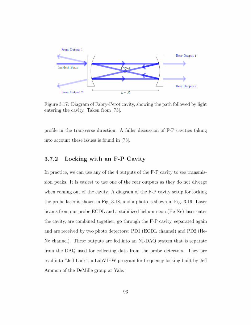
Figure 3.17: Diagram of Fabry-Perot cavity, showing the path followed by lightentering the cavity. Taken from [73].
profile in the transverse direction. A fuller discussion of F-P cavities taking
into account these issues is found in [73].
3.7.2 Locking with an F-P Cavity
In practice, we can use any of the 4 outputs of the F-P cavity to see transmis-
sion peaks. It is easiest to use one of the rear outputs as they do not diverge
when coming out of the cavity. A diagram of the F-P cavity setup for locking
the probe laser is shown in Fig. 3.18, and a photo is shown in Fig. 3.19. Laser
beams from our probe ECDL and a stabilized helium-neon (He-Ne) laser enter
the cavity, are combined together, go through the F-P cavity, separated again
and are received by two photo detectors: PD1 (ECDL channel) and PD2 (He-
Ne channel). These outputs are fed into an NI-DAQ system that is separate
from the DAQ used for collecting data from the probe detectors. They are
read into “Jeff Lock”, a LabVIEW program for frequency locking built by Jeff
Ammon of the DeMille group at Yale.
93
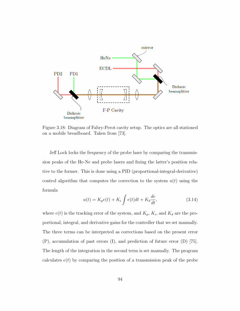
Figure 3.18: Diagram of Fabry-Perot cavity setup. The optics are all stationedon a mobile breadboard. Taken from [73].
Jeff Lock locks the frequency of the probe laser by comparing the transmis-
sion peaks of the He-Ne and probe lasers and fixing the latter’s position rela-
tive to the former. This is done using a PID (proportional-integral-derivative)
control algorithm that computes the correction to the system u(t) using the
formula
u(t) = Kpe(t) +Ki
∫e(t)dt+Kd
de
dt, (3.14)
where e(t) is the tracking error of the system, and Kp, Ki, and Kd are the pro-
portional, integral, and derivative gains for the controller that we set manually.
The three terms can be interpreted as corrections based on the present error
(P), accumulation of past errors (I), and prediction of future error (D) [75].
The length of the integration in the second term is set manually. The program
calculates e(t) by comparing the position of a transmission peak of the probe
94
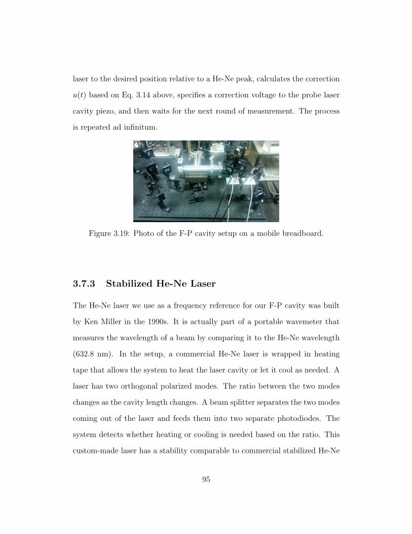
laser to the desired position relative to a He-Ne peak, calculates the correction
u(t) based on Eq. 3.14 above, specifies a correction voltage to the probe laser
cavity piezo, and then waits for the next round of measurement. The process
is repeated ad infinitum.
Figure 3.19: Photo of the F-P cavity setup on a mobile breadboard.
3.7.3 Stabilized He-Ne Laser
The He-Ne laser we use as a frequency reference for our F-P cavity was built
by Ken Miller in the 1990s. It is actually part of a portable wavemeter that
measures the wavelength of a beam by comparing it to the He-Ne wavelength
(632.8 nm). In the setup, a commercial He-Ne laser is wrapped in heating
tape that allows the system to heat the laser cavity or let it cool as needed. A
laser has two orthogonal polarized modes. The ratio between the two modes
changes as the cavity length changes. A beam splitter separates the two modes
coming out of the laser and feeds them into two separate photodiodes. The
system detects whether heating or cooling is needed based on the ratio. This
custom-made laser has a stability comparable to commercial stabilized He-Ne
95
lasers (on the order of several MHz).
3.8 Summary
We have now completed explaining all of the hardware components of our
experiment which are needed to accomplish our main task, which is to track the
precession frequency of the Cs atoms in the vapor cells by optical pumping and
probing. The next chapter will discuss the more programmatic and software
aspects of the system, as well as details on the procedures when running on
both PTP and CPP.
96
Chapter 4
Running Procedures
In this chapter, we shall discuss in more detail the actual protocols and stan-
dard procedures we perform when we run the experiment in its current con-
figuration using the test apparatus. We will also describe some important
features of the LabView programs we use to control the experiment. Here we
shall mainly cover the different procedures used for running in the PTP and
CPP schemes. A more thorough description of the general operating procedure
is in Appendix B.
4.1 Operating on CPP
First we will discuss the specifics of the procedure used to operate using CPP
mode. This comprises of firstly setting up the hardware, and secondly execut-
ing the LabView program to collect the data.
97
4.1.1 Setup
We first turn on the Stanford DS-345 function generator. This function gen-
erator is connected to the computer via a GPIB (IEEE-488) cable and can
generate a waveform of any arbitrary shape programmed by the computer.
Typically, we make it generate square waves with a duty cycle of 20% and an
amplitude of 1.0 V. An offset of half the amplitude is applied so that the actual
modulation is centered at 1.0 V instead of 0 V as the signal amplifier cannot
operate at negative voltages. Besides this, we usually also have an additional
0.02 V offset to further prevent excursions into negative voltages.
We turn on the two dual-phase SRS SR850 lock-in amplifiers. They are
connected to the computer via GPIB connectors. One of the lock ins (in our
case, the one connected for the bottom cell) actually provides the frequency to
the DS345 function generator: we set the DS345 to “burst mode” and connect
the frequency output from the SR850 to the DS345’s external trigger channel.
Burst mode makes the function generator generate a wave upon receiving a
rising slope signal from the external trigger. It is also possible to make function
generator itself set the frequency, but this method was chosen as it made it
possible for the lock-ins to operate using an internal reference frequency. The
waves from the function generator are sent to the signal amplifier, amplified
to several hundred volts, and sent to the Pockels cell, creating a continuous
modulation on the pump beam.
The dual phase lock-ins are connected to the DIFF channels from the
two probe photodetectors (one for each Cs cell). The principles of operation
for dual-phase lock-ins are similar to the single-phase ones discussed in Ap-
98
pendix A. The difference is that there are two PSD outputs. The first PSD is
the same as in Eq. A.4, but in the second PSD, the signal is multiplied with
the reference frequency shifted by π/2 [76]:
VPSD1 =1
2VsigVL cos(θsig − θref) ≈ Vsig cos θ = X, (4.1)
VPSD2 =1
2VsigVL sin(θsig − θref) ≈ Vsig sin θ = Y, (4.2)
(4.3)
where θ = θsig − θref. We thus have two outputs X and Y , which can also be
converted to polar coordinates R and θ. R becomes a measure of the signal
amplitude that is independent of the phase. In practice, we seek to maximize
R to get the most signal. This is how we detect the Larmor frequency: by
manually scanning the frequency of the bottom lock-in and seeing which gives
the highest value of R. Scanning over a fairly large range will result in a
Lorentzian curve that peaks at the Larmor frequency. θ, on the other hand,
will trace out an arctangent curve, which is expected as from Eqs. 4.2 and 4.3,
θ = arctan (Y/X).
4.1.2 Data Collection
The first data collection run begins with a sensitivity test that calibrates how
much change in frequency does an amount of change in phase correspond to,
or in other words finding df/dθ. Once the pump is modulated at the Larmor
frequency, the phase is set to zero. This is to ensure that we are operating in
the middle, approximately linear region of the arctangent curve. Initial zeroing
99
of phase enables us to easily detect changes in the phase; the absolute value
of the phase is arbitrary and meaningless in the experiment. The sensitivity
test occurs by changing the frequency to 0.5 Hz above and below the Larmor
frequency and seeing how the phase changes. The resulting slope becomes the
sensitivity. Typically, with the bottom “brown spot” and top “short stem”
vapor cells in the apparatus currently (April 2015), we obtain a sensitivity of
∼30 degrees/Hz for the bottom cell and ∼15 degrees/Hz for the top cell, which
makes sense as the bottom cell lifetime is roughly twice that of the top cell.
These sensitivity values can be used to convert changes in phase to changes in
frequency, and thus make it possible to compare with the results from PTP.
The actual data collection then commences. We usually set the lock-ins so
that they integrate the data received over a period of 60 ms into one single data
point that is sent to the computer. There is a pause of 300 ms between each
data point to prevent the lock-ins from being overwhelmed with commands.
Together with the time it takes for the GPIB to respond and other software
delays, it typically takes a total time of tdata ≈ 1.1 s for each data point. The
LabView program for CPP collects the data for R and θ, and also records
all the other settings of the experiment (frequency, amplitude, duty cycle,
etc.). Usually when testing for systematics, we take 20 points with the system
configured to a certain setting before changing it. The LabView program
automatically calculates important data from the set, mainly the standard
deviation and mean of the phase. Even when operating in this scheme, we
also record the 6 outputs of the probe detector (PD1, PD2, DIFF for top and
bottom cells) and 2 outputs from the pump monitor photodetectors (top and
100
bottom). These are connected to the computer via the NI PCIe-6361 DAQ
system.
4.2 Operating on PTP
We shall now discuss the specifics of the procedure used in operating using
the PTP scheme. In contrast to CPP, most of the commands and voltages
are generated directly by the DAQ system, so there are few external hardware
components that are used other than the DAQ.
When we want to operate on PTP, we first flip a switch so that the signal
amplifier input is connected to an output channel from the NI PCIe-6361 DAQ
system. For each pump-probe cycle, the LabView program digitally generates
a finite number of square pulses at the Larmor frequency. Usually we use a
20% duty cycle like with the CPP method. The waves are sent to the DAQ at
a writing frequency of 100 kHz. The DAQ sends them to the signal amplifier
which then relays them to the Pockels cell, causing pump modulation. Usually,
we pump the cell for 200 ms, resulting in about 400 waves. This is enough to
fully pump the atoms to a stable level of polarization.1
The output of the DAQ is also connected back to an input channel so that
we can continuously monitor the waves we are sending in to the DAQ. More
importantly, they are connected to an external trigger channel on the DAQ
that tells it when to start collecting input data from the probe detectors. It
is important that this be consistent, in order for all the traces for each pump-
1We will later discover that this may not be sufficient to fully reach equilibrium, causingissues when testing for systematics.
101
probe cycle to line up properly when they are averaged.2
After the pumping is finished, the output voltage on the DAQ is set to an
end value, usually zero.3 Usually we set the length of a pump-probe cycle to
600 ms (= tdata), such that the probing is done for 400 ms after the pumping
stops. During this time, the DAQ is instructed to read the input from the 6
channels of the probe detector outputs and the 2 pump monitors at a rate of
10 kHz. This results in 6000 points being recorded, and a decay curve like
Fig. 2.10.
The LabView program then takes the decaying portion of the curve (af-
ter the pumping stops, which is 4000 points long) and fits a function of the
form of Eq. 2.62 using the Levenberg-Marquardt algorithm (also known as the
Damped Least Squares method). We can choose how many points to actually
fit. Usually we don’t take all 4000 points, but the first 1000 or 2000, because
attempting to fit the portion when the polarization has largely decayed will
only worsen the fit.4 The fit parameters are recorded along with a host of other
parameters and data. The most important piece of data is the fit parameter
A1 which gives us the Larmor frequency of the atom. After a pump-probe
cycle is finished, the program immediately starts a new one and repeats as
needed.
As in CPP mode, we usually run PTP in batches of 20 points each. The
2This was very important in the early stages when we determined the Larmor frequencyby averaging a number of traces and then fitting a curve to it using Mathematica.
3We have found that this does not always result in the value read from the pump monitorbeing exactly zero, and so might investigate setting it to a larger or smaller value in thefuture.
4Later we will discover that slightly altering the number of points to fit will also slightlyshift the fitted frequency, which becomes another problem bringing the veracity of the fittedfrequency into question, and certainly worthy of deeper investigation.
102
program then calculates the mean and SD of the fit parameters. There is
also an option to save the individual traces for possible later additional data
analysis. Usually we only save the decaying portion, as saving complete traces
takes up a lot of hard disk space.
103

Chapter 5
Investigations Using the PTP
Scheme
In this chapter, we shall report the results of our investigations using the
pump-then-probe scheme, which we shall discuss before CPP because we did
the final analysis roughly in this order. All of the measurements are done using
the two-cell stack setup described in Ch. 3 and 4, with the “brown dot” cell at
the bottom and the “short stem” cell on top. The typical lifetimes were ∼43
ms for the top cell and ∼101 ms for the bottom cell.
5.1 Statistical Noise Measurements
The key to probing LRSSIs using our experiment is to monitor changes in the
spin precession frequency of the atoms with time. Thus the first task we did
was to measure the typical noise level of the frequency measurements over a
short period of time and see whether it is small enough to fulfill the sensitivity
104
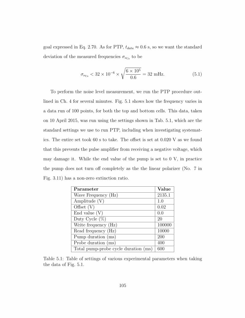
goal expressed in Eq. 2.70. As for PTP, tdata ≈ 0.6 s, so we want the standard
deviation of the measured frequencies σνCsto be
σνCs< 32× 10−6 ×
√6× 10⁵
0.6= 32 mHz. (5.1)
To perform the noise level measurement, we run the PTP procedure out-
lined in Ch. 4 for several minutes. Fig. 5.1 shows how the frequency varies in
a data run of 100 points, for both the top and bottom cells. This data, taken
on 10 April 2015, was run using the settings shown in Tab. 5.1, which are the
standard settings we use to run PTP, including when investigating systemat-
ics. The entire set took 60 s to take. The offset is set at 0.020 V as we found
that this prevents the pulse amplifier from receiving a negative voltage, which
may damage it. While the end value of the pump is set to 0 V, in practice
the pump does not turn off completely as the the linear polarizer (No. 7 in
Fig. 3.11) has a non-zero extinction ratio.
Parameter ValueWave Frequency (Hz) 2135.1Amplitude (V) 1.0Offset (V) 0.02End value (V) 0.0Duty Cycle (%) 20Write frequency (Hz) 100000Read frequency (Hz) 10000Pump duration (ms) 200Probe duration (ms) 400Total pump-probe cycle duration (ms) 600
Table 5.1: Table of settings of various experimental parameters when takingthe data of Fig. 5.1.
105
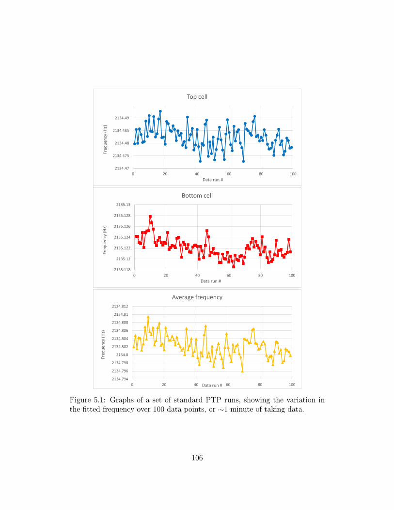
2134.47
2134.475
2134.48
2134.485
2134.49
0 20 40 60 80 100
Freq
uen
cy (
Hz)
Data run #
Top cell
2135.118
2135.12
2135.122
2135.124
2135.126
2135.128
2135.13
0 20 40 60 80 100
Freq
uen
cy (
Hz)
Data run #
Bottom cell
2134.794
2134.796
2134.798
2134.8
2134.802
2134.804
2134.806
2134.808
2134.81
2134.812
0 20 40 60 80 100
Freq
uen
cy (
Hz)
Data run #
Average frequency
Figure 5.1: Graphs of a set of standard PTP runs, showing the variation inthe fitted frequency over 100 data points, or ∼1 minute of taking data.
106
From this, we calculate the mean frequencies
νtop = 2134.482 Hz, (5.2)
νbot = 2135.122 Hz, (5.3)
with the standard deviations
σtop = 4.4 mHz, (5.4)
σbot = 1.8 mHz. (5.5)
Now, we will be looking at the average frequency between the two Cs cells.
The standard deviation of the average frequency between the top and bottom
cells, σav, is
σav = 2.6 mHz, (5.6)
which is well within the range mandated by Eq. 5.1, so the noise level for
PTP is statistically much better than the target sensitivity. When we take the
standard deviation of the difference frequency σdiff, we find
σdiff = 4.0 mHz, (5.7)
which is on the same level as Eq. 5.5. This indicates that the noise is not com-
mon mode noise, and may come from other sources such as the fitting process
(as we will discuss later). This brings us to the next step of investigation,
which is testing for systematics.
107
5.2 PTP Systematics Testing: Overview
The accuracy of an experiment can never be better than the systematic error.
The low level of noise in Eq. 5.6 would be futile if it turned out that our
frequency could easily vary due to changes in some experimental parameters
when taking data. The actual experiment will involve taking data in two
table positions, and there is a large risk of things systematically changing due
to the table rotation. We investigate this risk by artificially varying several
experimental parameters one at a time and seeing how much the frequency
varies, resulting in graphs of systematics. We then estimate how much we
can keep each experimental parameter constant. We will do this mainly based
on our past experience with Gen I. From this, we hope to find a region in
the graph where the slope of the measured frequency is small enough so that
the total variation in frequency in that region is smaller than the ultimate
sensitivity goal of 32 µHz (Eq. 2.68). If we can find such a region and operate
our experiment in it, then that particular systematic will not be a problem for
us. For the case of some parameters like pump frequency, we have no choice
of operating region (as we will have to pump at line center).
The four main parameters that we vary for both PTP and CPP are pump
intensity, pump frequency, probe intensity, and probe frequency. For CPP, it
is also important to investigate the effects of changing the angle between the
pump and probe beams. For PTP, as the pump beam is turned off during the
probing, we expect that the measured frequency should be relatively immune
to changes due to parameter changes in the pump. Changes to the pump
may affect the amplitude of the fit, but the Larmor frequency should stay the
108
same as we are not affecting the magnetic field. When varying the parameter,
we often increased the value up to a point and then decreased it back, to
counteract any natural drifts occurring by e.g., thermal fluctuations in the
room, which have a time scale of 20-30 minutes, about the time scale needed
to take the data.
5.3 Investigating Changes in Pump Intensity
We shall start by investigating the pump intensity. Pump intensity in PTP
can be varied in several ways. One can artificially increase the offset, am-
plitude, or the duty cycle of the wave generated from the DAQ, as all of
these effectively decide how much light is “given” to the atom. It is more
straightforward, however, to use an attenuator/filter, as we did with the neu-
tral density aluminum-coated attenuator wheel described in Ch. 3.5.5. We
collected data for 20 runs, changed the pump intensity by spinning the wheel,
waited a few seconds for things to settle down, resumed collecting data for
another 20 runs, and so on. The intensity of the pump was measured by tak-
ing the last 100 points in the pump monitor before pumping was stopped and
finding the peak-to-peak values of the pump modulation by using the Extract
Single Tone Information VI in LabVIEW, which uses a fast Fourier transform
method to accomplish this. This quantity is proportional to the pump inten-
sity: a lower pump intensity would result in less spin polarization and thus a
smaller peak-to-peak amplitude in the pump modulation.
The results are shown in Fig. 5.2. As the intensity is increased, we see
109
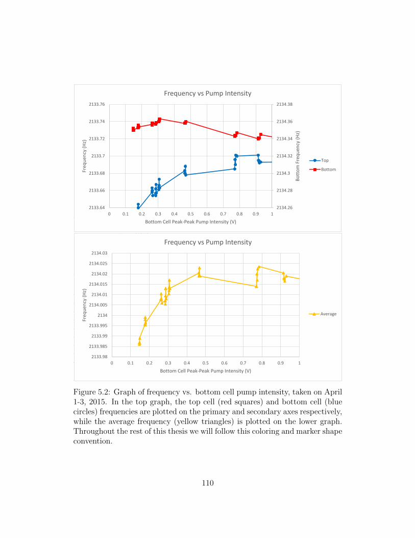
2134.6
Frequency vs Pump Intensity (ND wheel used)
2134.26
2134.28
2134.3
2134.32
2134.34
2134.36
2134.38
2133.64
2133.66
2133.68
2133.7
2133.72
2133.74
2133.76
0 0.1 0.2 0.3 0.4 0.5 0.6 0.7 0.8 0.9 1
Bo
tto
m F
req
uen
cy (
Hz)
Freq
uen
cy (
Hz)
Bottom Cell Peak-Peak Pump Intensity (V)
Frequency vs Pump Intensity
Top
Bottom
5 6 7 8 9
Chart Title
0.123
2133
2133.2
2133.4
2133.6
2133.8
2134
2134.2
2134.4
2134.6
0 0.1 0.2 0.3 0.4 0.5 0.6
Freq
uen
cy (
Hz)
Peak to Peak Pump intensity (Bottom)
Frequency vs Pump Intensity (ND wheel used)
2133.622 2134.352 -0.73
2133.72
2133.622
2133.98
2133.985
2133.99
2133.995
2134
2134.005
2134.01
2134.015
2134.02
2134.025
2134.03
0 0.1 0.2 0.3 0.4 0.5 0.6 0.7 0.8 0.9 1
Freq
uen
cy (
Hz)
Bottom Cell Peak-Peak Pump Intensity (V)
Frequency vs Pump Intensity
Average
Figure 5.2: Graph of frequency vs. bottom cell pump intensity, taken on April1-3, 2015. In the top graph, the top cell (red squares) and bottom cell (bluecircles) frequencies are plotted on the primary and secondary axes respectively,while the average frequency (yellow triangles) is plotted on the lower graph.Throughout the rest of this thesis we will follow this coloring and marker shapeconvention.
110
an increase in the average frequency that peters out starting at V ≈ 0.5 V.
From V = 0.5 − 0.7 V, the frequency is stable but has noise in the 10 mHz
range. This is likely the stable region that we can operate in. In Fig. 5.3
we fit a straight line to this region, which has the slope of 3(6) µHz/mV. As
the uncertainty of the slope is larger than the slope itself, we can regard it as
the systematic uncertainty itself. Thus, we have a systematic uncertainty of
6 µHz, or an order of magnitude lower than the ultimate sensitivity goal (32
µHz). Based on this rough assessment, we should not have to worry about
changes in pump intensity. However, the data in this stable region is still quite
noisy and spotty. Finer and more thorough scans of this region should be done
to more properly calculate the slope.
5.4 Investigating Changes in Pump Frequency
We shall now proceed to discuss the systematics test we ran for changes in
pump frequency. To vary the pump frequency, we unlock the pump and adjust
the bias voltage on the pump laser piezo in small increments. As the pump
is unlocked, the noise level is naturally higher. We can calibrate the x-axis
to frequency units by observing the error signal from the single phase SR510
lock-in amplifier, which follows the shape shown in Fig. A.2. The horizontal
distance between the peak and the valley surrounding the center is given by
the full width half maximum of the original absorption curve (Fig. A.1). This
111
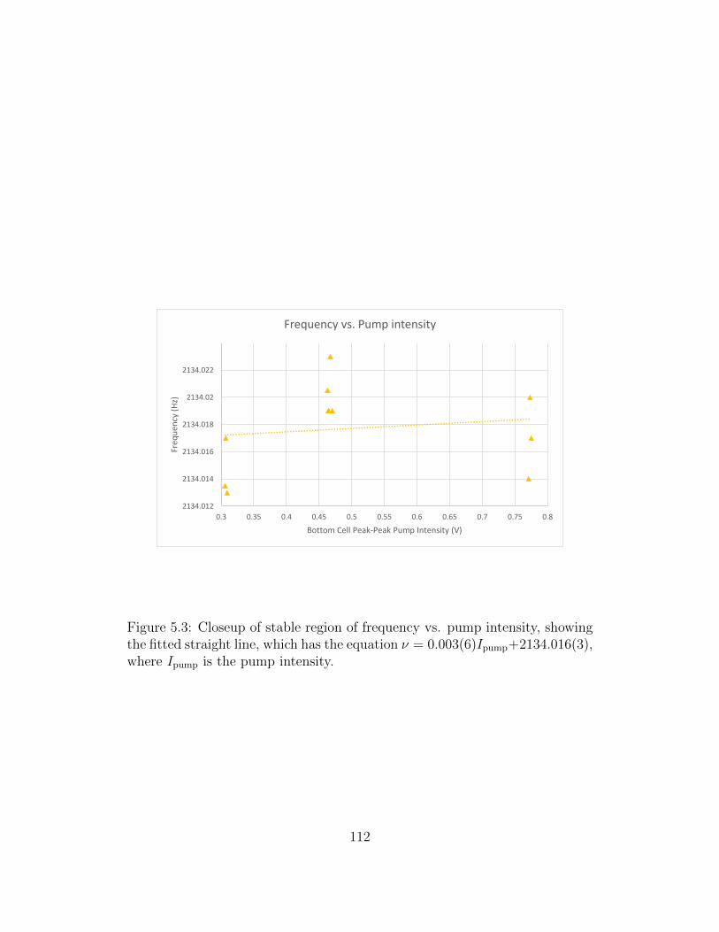
2134.012
2134.014
2134.016
2134.018
2134.02
2134.022
0.3 0.35 0.4 0.45 0.5 0.55 0.6 0.65 0.7 0.75 0.8
Freq
uen
cy (
Hz)
Bottom Cell Peak-Peak Pump Intensity (V)
Frequency vs. Pump intensity
Figure 5.3: Closeup of stable region of frequency vs. pump intensity, showingthe fitted straight line, which has the equation ν = 0.003(6)Ipump+2134.016(3),where Ipump is the pump intensity.
112
is known as the Doppler width, calculated by the formula
νFWHM =
√8kbT
mc2ν0, (5.8)
where T is the room temperature (∼300 K), m is the mass of a Cs atom
(≈ 2.21×10⁻²⁵ kg), and ν0 is the frequency of the line center (894 nm), giving
us νFWHM ≈ 365 MHz.
The results of our investigation using this calibrated x-axis are shown in
Fig. 5.4, which resembles a lopsided dispersion curve. Fig. 5.5 zooms in on the
central region near line center and fits a straight line to it. We find the slope
to be 0.21(2) mHz/MHz. We observe that when the pump is locked using the
frequency locking mechanism described in Appendix A, the error signal on the
lock-in has noise on the level of ∼1 unit. Meanwhile, the Doppler width of
∼365 Hz is ∼80 units wide, which means the pump frequency varies on the
level of ∼5 MHz. The actual noise in pump frequency during an experiment
will be even smaller, because we will be using saturated absorption, which
causes a sharp dip at line center in the Cs absorption profile that we lock to.
This significantly improves the robustness of the locking mechanism
The actual frequency shift between the two table positions is much smaller
than the noise level of the pump. In the Gen I experiment, we typically find
the ratio
∆νodd
∆νnoise
≈ 10−3, (5.9)
where ∆νodd is the table-dependent systematic shift and ∆νnoise is the pump
noise level. Assuming Gen II will exhibit similar behavior, we can estimate
113
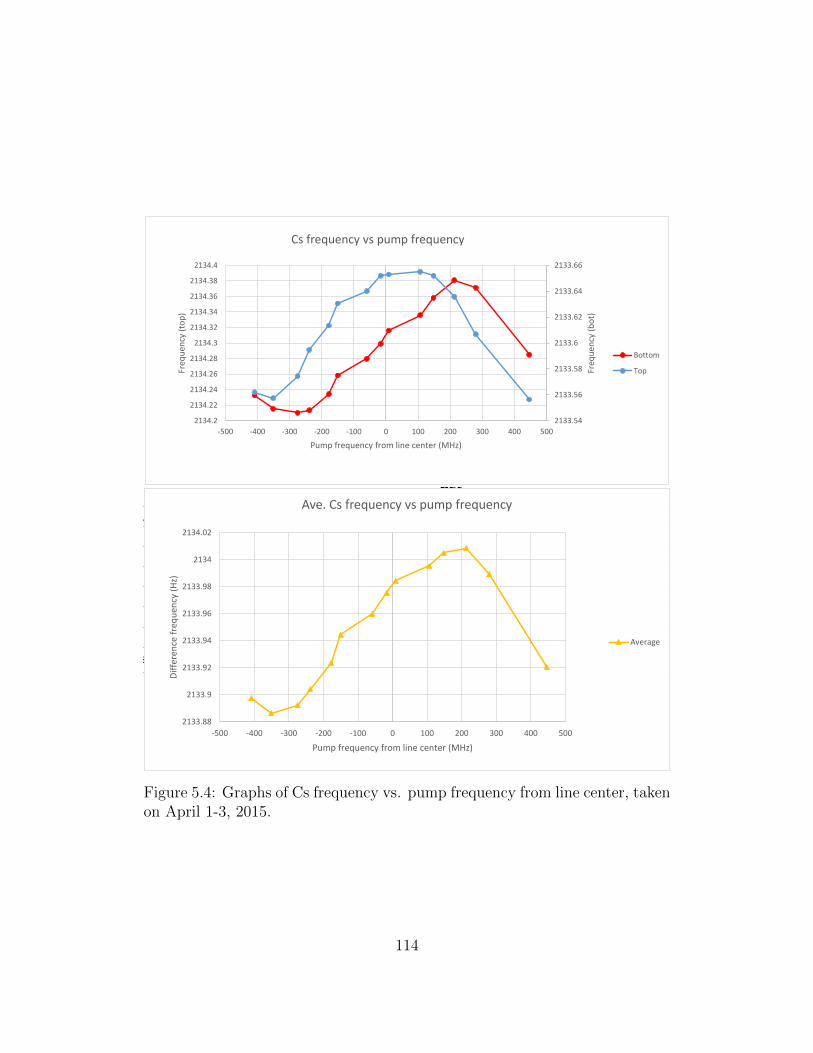
2133.54
2133.56
2133.58
2133.6
2133.62
2133.64
2133.66
2134.2
2134.22
2134.24
2134.26
2134.28
2134.3
2134.32
2134.34
2134.36
2134.38
2134.4
-500 -400 -300 -200 -100 0 100 200 300 400 500
Freq
uen
cy (
bo
t)
Freq
uen
cy (
top
)
Pump frequency from line center (MHz)
Cs frequency vs pump frequency
Bottom
Top
5 6 7 8 9 10 11 12 13 14 15 16 17 18 19 20 21 22 23 24 25 26 27
pzt
2133.88
2133.9
2133.92
2133.94
2133.96
2133.98
2134
2134.02
-500 -400 -300 -200 -100 0 100 200 300 400 500
Dif
fere
nce
fre
qu
ency
(H
z)
Pump frequency from line center (MHz)
Ave. Cs frequency vs pump frequency
Average
Figure 5.4: Graphs of Cs frequency vs. pump frequency from line center, takenon April 1-3, 2015.
114
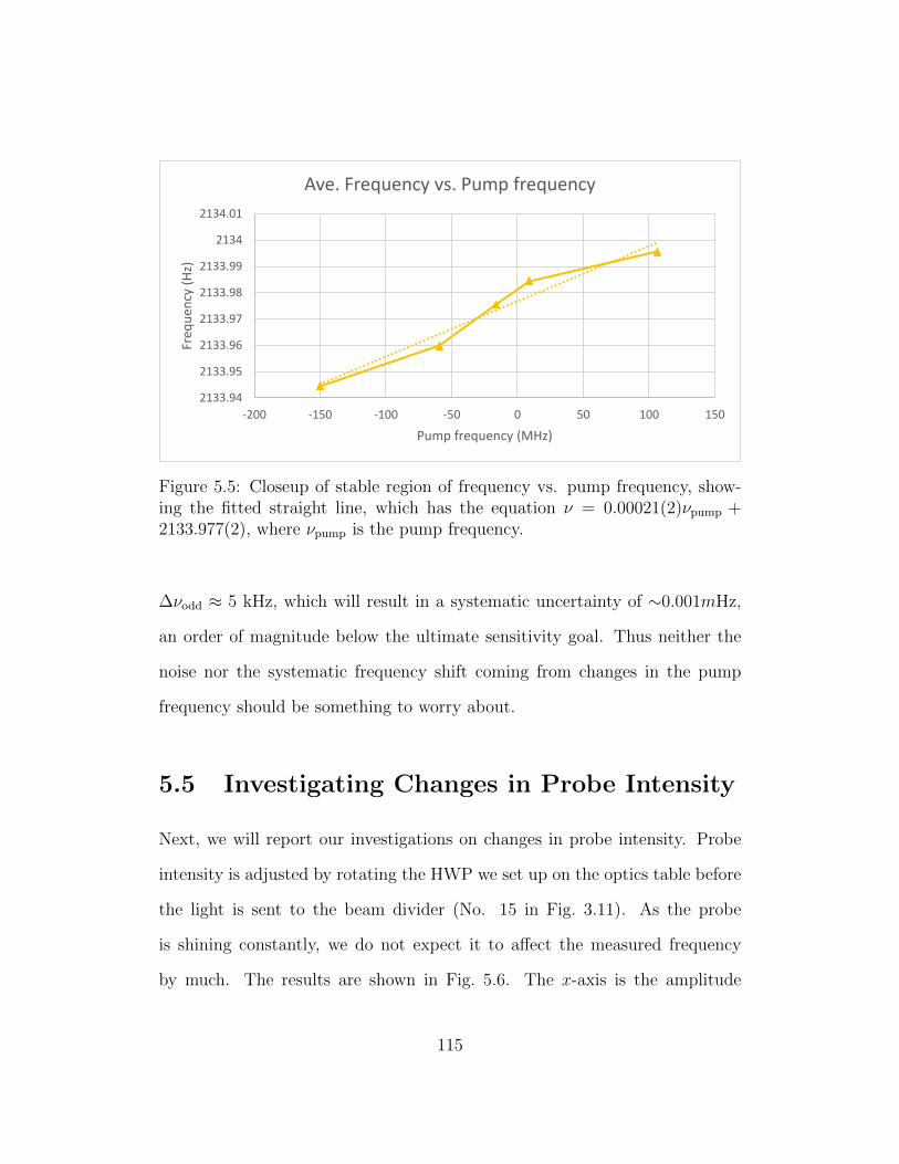
2133.94
2133.95
2133.96
2133.97
2133.98
2133.99
2134
2134.01
-200 -150 -100 -50 0 50 100 150
Freq
uen
cy (
Hz)
Pump frequency (MHz)
Ave. Frequency vs. Pump frequency
Figure 5.5: Closeup of stable region of frequency vs. pump frequency, show-ing the fitted straight line, which has the equation ν = 0.00021(2)νpump +2133.977(2), where νpump is the pump frequency.
∆νodd ≈ 5 kHz, which will result in a systematic uncertainty of ∼0.001mHz,
an order of magnitude below the ultimate sensitivity goal. Thus neither the
noise nor the systematic frequency shift coming from changes in the pump
frequency should be something to worry about.
5.5 Investigating Changes in Probe Intensity
Next, we will report our investigations on changes in probe intensity. Probe
intensity is adjusted by rotating the HWP we set up on the optics table before
the light is sent to the beam divider (No. 15 in Fig. 3.11). As the probe
is shining constantly, we do not expect it to affect the measured frequency
by much. The results are shown in Fig. 5.6. The x-axis is the amplitude
115
of the fit function of the bottom cell (fit parameter A3 in Eq. 2.62), which
correlates well with our adjustments on the HWP and thus is a good proxy of
probe intensity. At high intensities, this quantity saturates, but this is not a
problem as we normally already operate at near the maximum probe intensity
without saturation. 1 As the data is noisy over the entire range of intensities,
there is no particular region that is relatively stabler. Hence we fit a straight
line to all the points, giving a slope of 0.005(2) Hz/V = 5 µHz/mV. Assuming
again that we can keep the probe laser intensity stable to within ∼1 mV,
we will get a systematic uncertainty of 5 µHz, a factor of 6 better than the
sensitivity goal. Thus this systematic should also not be of much conern.
1The dual lock-ins have an input voltage limit that limits us from operating the probelaser at the fullest intensity.
116
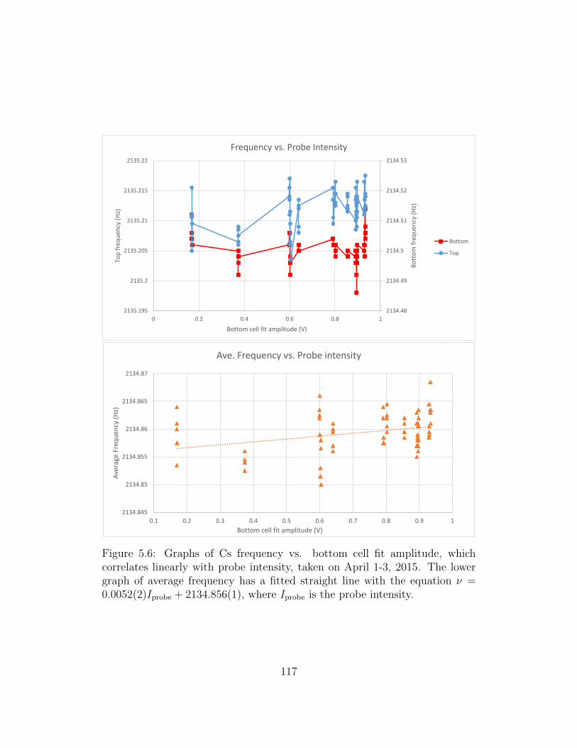
2134.48
2134.49
2134.5
2134.51
2134.52
2134.53
2135.195
2135.2
2135.205
2135.21
2135.215
2135.22
0 0.2 0.4 0.6 0.8 1
Bo
tto
m f
req
uen
cy (
Hz)
Top
fre
qu
ency
(H
z)
Bottom cell fit amplitude (V)
Frequency vs. Probe Intensity
Bottom
Top
2135.195
2135.2
2135.205
Top
fre
qu
ency
(H
z)
2134.845
2134.85
2134.855
2134.86
2134.865
2134.87
0.1 0.2 0.3 0.4 0.5 0.6 0.7 0.8 0.9 1
Ave
rage
Fre
qu
ency
(H
z)
Bottom cell fit amplitude (V)
Ave. Frequency vs. Probe intensity
Figure 5.6: Graphs of Cs frequency vs. bottom cell fit amplitude, whichcorrelates linearly with probe intensity, taken on April 1-3, 2015. The lowergraph of average frequency has a fitted straight line with the equation ν =0.0052(2)Iprobe + 2134.856(1), where Iprobe is the probe intensity.
117
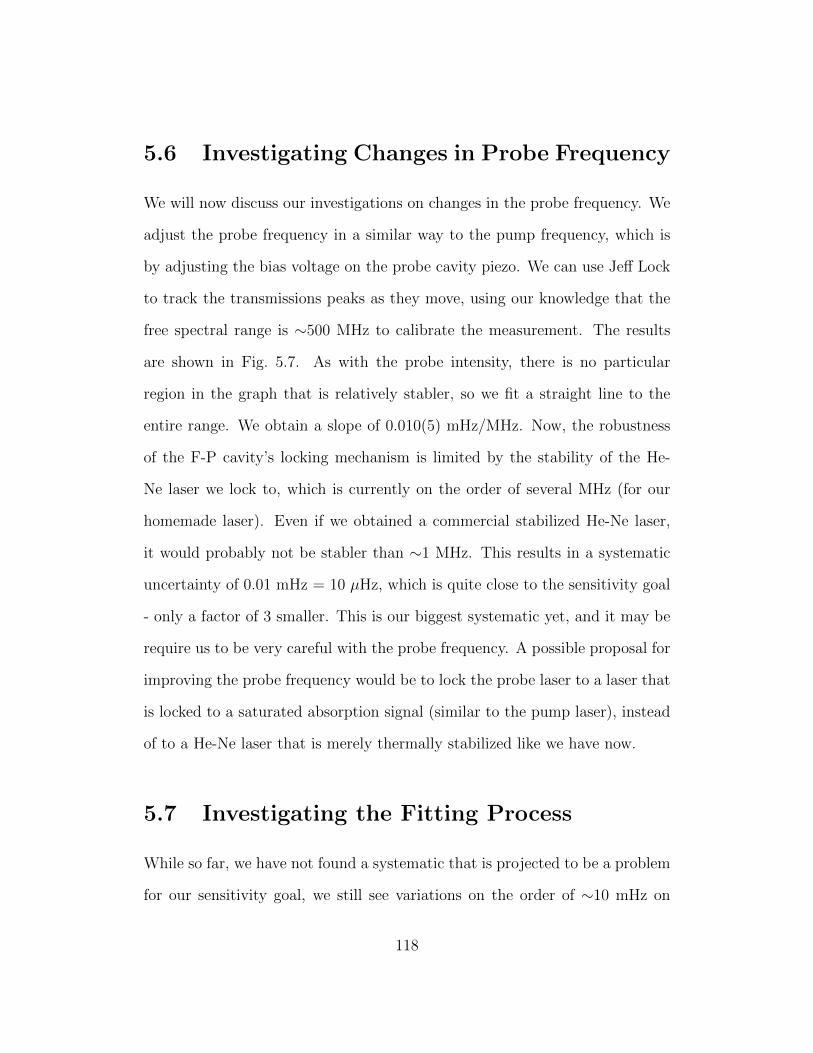
5.6 Investigating Changes in Probe Frequency
We will now discuss our investigations on changes in the probe frequency. We
adjust the probe frequency in a similar way to the pump frequency, which is
by adjusting the bias voltage on the probe cavity piezo. We can use Jeff Lock
to track the transmissions peaks as they move, using our knowledge that the
free spectral range is ∼500 MHz to calibrate the measurement. The results
are shown in Fig. 5.7. As with the probe intensity, there is no particular
region in the graph that is relatively stabler, so we fit a straight line to the
entire range. We obtain a slope of 0.010(5) mHz/MHz. Now, the robustness
of the F-P cavity’s locking mechanism is limited by the stability of the He-
Ne laser we lock to, which is currently on the order of several MHz (for our
homemade laser). Even if we obtained a commercial stabilized He-Ne laser,
it would probably not be stabler than ∼1 MHz. This results in a systematic
uncertainty of 0.01 mHz = 10 µHz, which is quite close to the sensitivity goal
- only a factor of 3 smaller. This is our biggest systematic yet, and it may be
require us to be very careful with the probe frequency. A possible proposal for
improving the probe frequency would be to lock the probe laser to a laser that
is locked to a saturated absorption signal (similar to the pump laser), instead
of to a He-Ne laser that is merely thermally stabilized like we have now.
5.7 Investigating the Fitting Process
While so far, we have not found a systematic that is projected to be a problem
for our sensitivity goal, we still see variations on the order of ∼10 mHz on
118
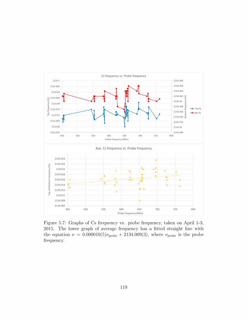
2134.348
2134.35
2134.352
2134.354
2134.356
2134.358
2134.36
2134.362
2134.364
2134.366
2134.368
2133.655
2133.66
2133.665
2133.67
2133.675
2133.68
2133.685
2133.69
2133.695
2133.7
450 500 550 600 650 700 750 800
Bo
tto
m f
req
uen
cy (H
z)
Top
fre
qu
ency
(H
z)
Probe frequency (MHz)
Cs frequency vs. Probe frequency
Top fq
Bot fq
2134.006
2134.008
2134.01
2134.012
2134.014
2134.016
2134.018
2134.02
2134.022
2134.024
450 500 550 600 650 700 750 800
Top
an
d b
ott
om
freq
uen
cy (
Hz)
Probe frequency (MHz)
Ave. Cs frequency vs. Probe frequency
Figure 5.7: Graphs of Cs frequency vs. probe frequency, taken on April 1-3,2015. The lower graph of average frequency has a fitted straight line withthe equation ν = 0.000010(5)νprobe + 2134.009(3), where νprobe is the probefrequency.
119
several systematics as we vary them over a large range. For example, in the
graphs of frequency vs. pump intensity (Fig. 5.2), we see a variation of ∼0.04
Hz over the entire range of pump intensity. This is slightly intriguing, as in
PTP, the pump is not shining when the atoms are being probed, so whatever
the net spin polarization of the system, they should decay while spinning at
the same Larmor frequency. We suspected that this shift may have to do with
problems with the Levenberg-Marquardt algorithm LabVIEW is using to fit
the curve. It is possible that the algorithm might have some dependency on
the initial amplitude of the decay being fitted. It is also possible that despite
having pumped for what we consider an ample amount of time (200 ms) for
the atoms to become fully polarized, there are still some small fluctuations in
the amplitude. Thus, this will result in small shifts in the fitted frequency even
though the actual precession frequency will be the same. Another possibility is
that the pump laser is not completely extinguished by the Pockels cell during
the probing stage. In this section, we shall report some of the investigations
that led us to be aware of potential limitations in the fitting algorithm.
5.7.1 Investigating Changes in Pump Duration
If the system is not fully polarized after 200 ms of pumping, a longer pump time
might make it stabler. Thus, if the fitting algorithm is dependent on the initial
amplitude as we theorized, we expect the fitted frequency to vary as we vary
the pump duration. In fact, we might expect the fitted frequency to stabilize as
the pump duration lengthens. So we performed tests where we varied the pump
duration specified to the DAQ, from extremely short to over several times the
120
regular duration. The results are shown in Fig. 5.8. Each point was taken 3-4
times to counteract noise. At extremely short pump durations, as expected,
the fitted frequency has a sharp increase. When the tpump > 100 ms, the
average frequency flattens out with a noise level of ∼0.01 Hz. However, if we
look at the individual plots of the top and bottom cells, starting at tpump = 100
ms, we see a modulation that is somewhat sinusoidal. This sinusoidal variation
seemed to indicate something to do with the algorithm, instead of a physical
effect.
As increasing the pump duration even longer would make PTP not fea-
sible, we became curious as to what would happen if we were to to try the
same investigation, but with double the amplitude of the wave sent out by the
DAQ. This effectively increases the overall pump intensity, equivalent to in-
creasing the driving force on the damped harmonic oscillator, hopefully making
it stabilize quicker. The results are shown in Fig. 5.9. Looking at the results
tpump < 100 ms, the average frequency varies by 0.02 Hz, a factor of 2 better
than when the amplitude was 1 V. In the individual plots for the two cells,
There is still an up-down pattern but it is less sinusoidal than before. This
indicates that it may be better to operate at slightly longer pump durations,
if we can afford the time, as the current tpump = 200 ms is just on the verge of
the stable region in the graph. We did not attempt even larger amplitudes of
the pump, as the pulse amplifier is unable to take amplitudes larger than 2 V.
121
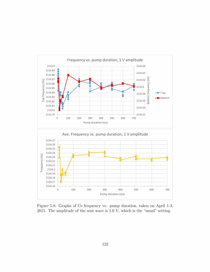
2134.52
2134.54
2134.56
2134.58
2134.6
2134.62
2134.64
2134.66
2133.79
2133.8
2133.81
2133.82
2133.83
2133.84
2133.85
2133.86
2133.87
2133.88
2133.89
2133.9
0 100 200 300 400 500 600 700
Bo
tto
m f
req
uen
cy (
Hz)
Top
fre
qu
ency
(H
z)
Pump duration (ms)
Frequency vs. pump duration, 1 V amplitude
Top
Bottom
2134.16
2134.17
2134.18
2134.19
2134.2
2134.21
2134.22
2134.23
2134.24
2134.25
2134.26
2134.27
0 100 200 300 400 500 600 700
Freq
uen
cy (
Hz)
Pump duration (ms)
Ave. Frequency vs. pump duration, 1 V amplitude
Figure 5.8: Graphs of Cs frequency vs. pump duration, taken on April 1-3,2015. The amplitude of the sent wave is 1.0 V, which is the “usual” setting.
122
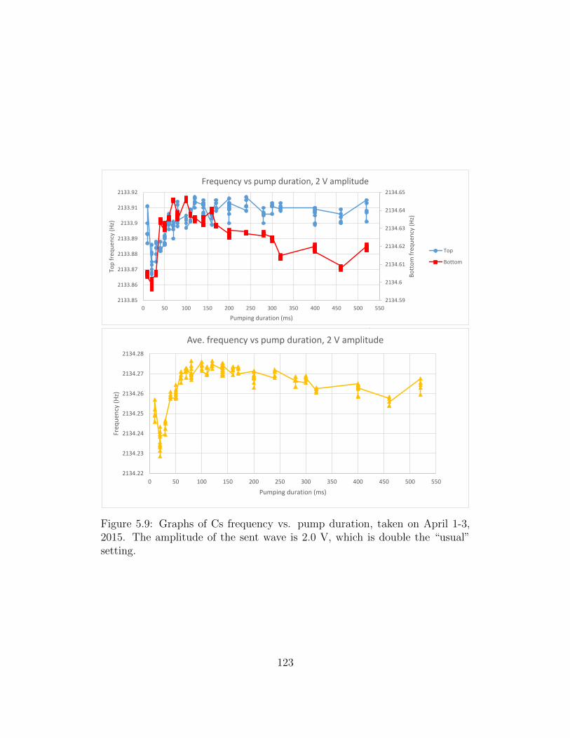
2134.59
2134.6
2134.61
2134.62
2134.63
2134.64
2134.65
2133.85
2133.86
2133.87
2133.88
2133.89
2133.9
2133.91
2133.92
0 50 100 150 200 250 300 350 400 450 500 550
Bo
tto
m f
req
uen
cy (
Hz)
Top
fre
qu
ency
(H
z)
Pumping duration (ms)
Frequency vs pump duration, 2 V amplitude
Top
Bottom
2134.22
2134.23
2134.24
2134.25
2134.26
2134.27
2134.28
0 50 100 150 200 250 300 350 400 450 500 550
Freq
uen
cy (
Hz)
Pumping duration (ms)
Ave. frequency vs pump duration, 2 V amplitude
Figure 5.9: Graphs of Cs frequency vs. pump duration, taken on April 1-3,2015. The amplitude of the sent wave is 2.0 V, which is double the “usual”setting.
123
5.7.2 Investigating Changes in Pump Modulation Fre-
quency
Another parameter we investigated was the pump modulation frequency. To
do this, we simply change the setting on the wave sent out to the DAQ.
This was done on the maximum amplitude of 2 V, to try to quickly saturate
the polarization of the system. The effect of this should be similar to pump
duration, in that the closer we get to the Larmor frequency, the fitted frequency
should become stabler. The results are shown in Fig. 5.10, and they are
surprising as the average frequency graph resembles a dispersion curve in the
region of the Larmor frequency. When we do finer increments around the
actual Larmor frequency (Fig. 5.11), we can clearly see the fit frequency of
the top and bottom cells crisscrossing, meeting at approximately the Larmor
frequency. This is a mystery that we are still investigating. What is important,
though is to keep the modulation frequency constant, which is not difficult to
do with our DAQ.
124
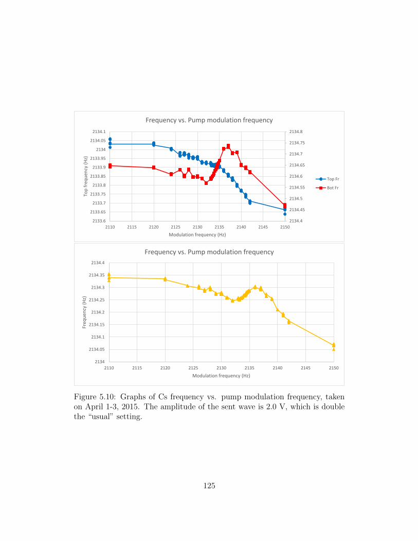
2134.4
2134.45
2134.5
2134.55
2134.6
2134.65
2134.7
2134.75
2134.8
2133.6
2133.65
2133.7
2133.75
2133.8
2133.85
2133.9
2133.95
2134
2134.05
2134.1
2110 2115 2120 2125 2130 2135 2140 2145 2150
Top
fre
qu
ency
(H
z)
Modulation frequency (Hz)
Frequency vs. Pump modulation frequency
Top Fr
Bot Fr
2134
2134.05
2134.1
2134.15
2134.2
2134.25
2134.3
2134.35
2134.4
2110 2115 2120 2125 2130 2135 2140 2145 2150
Freq
uen
cy (
Hz)
Modulation frequency (Hz)
Frequency vs. Pump modulation frequency
Figure 5.10: Graphs of Cs frequency vs. pump modulation frequency, takenon April 1-3, 2015. The amplitude of the sent wave is 2.0 V, which is doublethe “usual” setting.
125
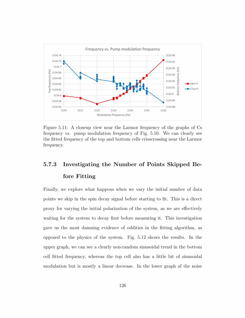
2133.88
2133.89
2133.9
2133.91
2133.92
2133.93
2133.94
2133.95
2133.96
2134.56
2134.58
2134.6
2134.62
2134.64
2134.66
2134.68
2134.7
2134.72
2134.74
2130 2131 2132 2133 2134 2135 2136
Bo
tto
m f
req
uen
cy (
Hz)
Top
fre
qu
ency
(H
z)
Modulation frequency (Hz)
Frequency vs. Pump modulation frequency
Bot Fr
Top Fr
Figure 5.11: A closeup view near the Larmor frequency of the graphs of Csfrequency vs. pump modulation frequency of Fig. 5.10. We can clearly seethe fitted frequency of the top and bottom cells crisscrossing near the Larmorfrequency.
5.7.3 Investigating the Number of Points Skipped Be-
fore Fitting
Finally, we explore what happens when we vary the initial number of data
points we skip in the spin decay signal before starting to fit. This is a direct
proxy for varying the initial polarization of the system, as we are effectively
waiting for the system to decay first before measuring it. This investigation
gave us the most damning evidence of oddities in the fitting algorithm, as
opposed to the physics of the system. Fig. 5.12 shows the results. In the
upper graph, we can see a clearly non-random sinusoidal trend in the bottom
cell fitted frequency, whereas the top cell also has a little bit of sinusoidal
modulation but is mostly a linear decrease. In the lower graph of the noise
126
level (σ) against points skipped, for the bottom cell we also see a sinusoidal
variation, although they are all within 1.5-2.0 mHz, which is the typical level
for the bottom cell. For the top cell, σ slowly increases from 3 mHz to 4 mHz
over a variation of 0-200 points skipped (or 0-20 ms before fitting). This clearly
sinusoidal behavior is definitely something to do with the fitting algorithm.
Thus, we need to more thoroughly investigate the fitting process before we
put our full faith in it. On the other hand, it is perhaps more important to
ensure that once we settle on a fitting routine, we stick to its exact settings
and parameters for all of our data analysis.
127
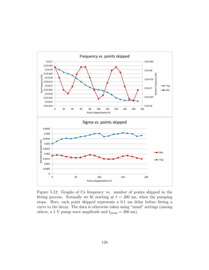
2134.36
2134.365
2134.37
2134.375
2134.38
2134.385
2133.645
2133.65
2133.655
2133.66
2133.665
2133.67
2133.675
2133.68
2133.685
2133.69
2133.695
2133.7
0 20 40 60 80 100 120 140 160 180 200
Bo
tto
m F
req
uen
cy (
Hz)
Top
Fre
qu
ency
(H
z)
Points skipped before fit
Frequency vs. points skipped
Top
Bot
0
0.0005
0.001
0.0015
0.002
0.0025
0.003
0.0035
0.004
0.0045
0 50 100 150 200
Stan
dar
d d
evia
tio
n (
Hz)
Points skipped before fit
Sigma vs. points skipped
Bot
Top
Figure 5.12: Graphs of Cs frequency vs. number of points skipped in thefitting process. Normally we fit starting at t = 200 ms, when the pumpingstops. Here, each point skipped represents a 0.1 ms delay before fitting acurve to the decay. The data is otherwise taken using “usual” settings (amongothers, a 1 V pump wave amplitude and tpump = 200 ms).
128
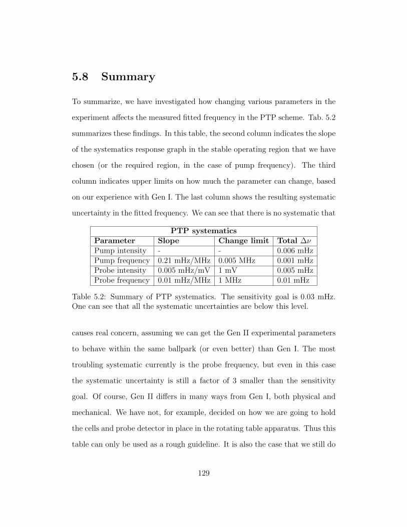
5.8 Summary
To summarize, we have investigated how changing various parameters in the
experiment affects the measured fitted frequency in the PTP scheme. Tab. 5.2
summarizes these findings. In this table, the second column indicates the slope
of the systematics response graph in the stable operating region that we have
chosen (or the required region, in the case of pump frequency). The third
column indicates upper limits on how much the parameter can change, based
on our experience with Gen I. The last column shows the resulting systematic
uncertainty in the fitted frequency. We can see that there is no systematic that
PTP systematicsParameter Slope Change limit Total ∆νPump intensity - - 0.006 mHzPump frequency 0.21 mHz/MHz 0.005 MHz 0.001 mHzProbe intensity 0.005 mHz/mV 1 mV 0.005 mHzProbe frequency 0.01 mHz/MHz 1 MHz 0.01 mHz
Table 5.2: Summary of PTP systematics. The sensitivity goal is 0.03 mHz.One can see that all the systematic uncertainties are below this level.
causes real concern, assuming we can get the Gen II experimental parameters
to behave within the same ballpark (or even better) than Gen I. The most
troubling systematic currently is the probe frequency, but even in this case
the systematic uncertainty is still a factor of 3 smaller than the sensitivity
goal. Of course, Gen II differs in many ways from Gen I, both physical and
mechanical. We have not, for example, decided on how we are going to hold
the cells and probe detector in place in the rotating table apparatus. Thus this
table can only be used as a rough guideline. It is also the case that we still do
129
not fully understand why changing anything about the pump affects the fitted
frequency measurably. As we have seen in Sec. 5.7, there are peculiarities
about the fitting algorithm that must be investigated in greater depth if we
are to go forward with PTP as a method. Also, finer and more thorough
scans of the designated stable operating regions for each parameter must be
performed, to better determine the slopes of the graphs.
130
Chapter 6
Investigations Using the CPP
Scheme
In this chapter, we shall report the results of investigations using the con-
tinuous pumping-probing (CPP) scheme. Similar to our PTP investigations,
we did a basic noise level measurement, then commenced doing systematics
investigations in order to decide on how suitable it is for our purposes. The
cells used are the same as when investigating PTP: the “brown dot” cell at
the bottom and the “short stem cell” on top.
6.1 Statistical Noise Measurements
To measure the basic noise level, we ran the apparatus on CPP for several
minutes and measured the noise on the phase of the top and bottom cells
using the standard procedure outlined in Ch. 4. Unlike PTP, there are not so
many settings when running on CPP. This data set was taken using a Larmor
131
frequency of 2135.1 Hz, 60 ms integraiton time, 20% duty cycle, 0.02 V offset
(to prevent the signal amplifier from receiving negative voltage), and 1.0 V
amplitude. We must note that because for CPP, tdata = 1.1 s, which is almost
twice that of PTP (mainly due to our efforts to prevent the dual-phase lock-ins
from being overloaded with commands), the sensitivity goal is slightly more
stringent, namely
σνCs< 32× 10−6 ×
√6× 10⁵
1.1= 23 mHz. (6.1)
Fig. 6.1 shows a typical data set from a noise measurement run. In this
example, the sensitivities η of the top and bottom were measured out (using
the calibration method of Sec. 4.1.2) to be
ηtop = 14 degrees/Hz, (6.2)
ηbot = 31 degrees/Hz, (6.3)
which are typical values for the sensitivity, reflecting the fact that the bottom
cell lifetime is roughly twice of the top cell lifetime. To calculate the average
frequency νdiff between the two cells, we must scale the phase measurements
by these sensitivities, as expressed in the formula
νave =1
2
(θtop
ηtop
+θbot
ηbot
). (6.4)
The mean absolute value of the phase or frequency of the data set is not
important as it is completely arbitrary, depending on when and where we set
132
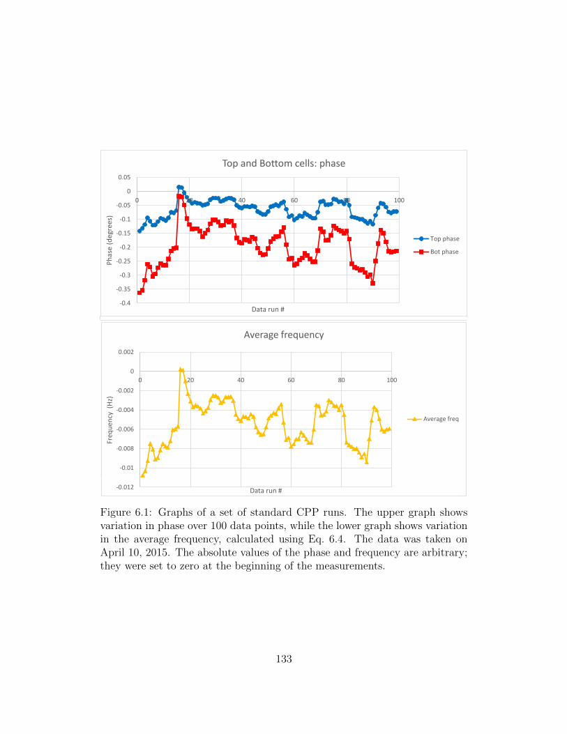
-0.4
-0.35
-0.3
-0.25
-0.2
-0.15
-0.1
-0.05
0
0.05
0 20 40 60 80 100
Ph
ase
(deg
rees
)
Data run #
Top and Bottom cells: phase
Top phase
Bot phase
Phase difference
0.05
Top and Bottom cells: phase-0.012
-0.01
-0.008
-0.006
-0.004
-0.002
0
0.002
0 20 40 60 80 100
Freq
uen
cy (
Hz)
Data run #
Average frequency
Average freq
Figure 6.1: Graphs of a set of standard CPP runs. The upper graph showsvariation in phase over 100 data points, while the lower graph shows variationin the average frequency, calculated using Eq. 6.4. The data was taken onApril 10, 2015. The absolute values of the phase and frequency are arbitrary;they were set to zero at the beginning of the measurements.
133
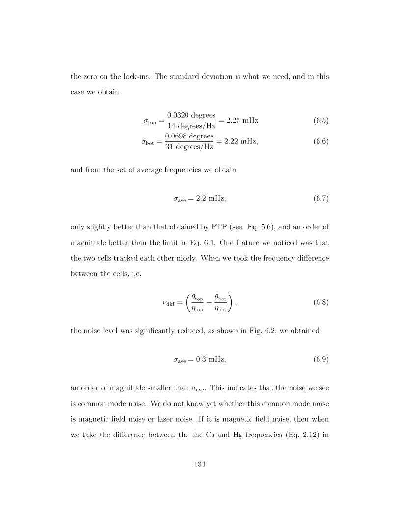
the zero on the lock-ins. The standard deviation is what we need, and in this
case we obtain
σtop =0.0320 degrees
14 degrees/Hz= 2.25 mHz (6.5)
σbot =0.0698 degrees
31 degrees/Hz= 2.22 mHz, (6.6)
and from the set of average frequencies we obtain
σave = 2.2 mHz, (6.7)
only slightly better than that obtained by PTP (see. Eq. 5.6), and an order of
magnitude better than the limit in Eq. 6.1. One feature we noticed was that
the two cells tracked each other nicely. When we took the frequency difference
between the cells, i.e.
νdiff =
(θtop
ηtop
− θbot
ηbot
), (6.8)
the noise level was significantly reduced, as shown in Fig. 6.2; we obtained
σave = 0.3 mHz, (6.9)
an order of magnitude smaller than σave. This indicates that the noise we see
is common mode noise. We do not know yet whether this common mode noise
is magnetic field noise or laser noise. If it is magnetic field noise, then when
we take the difference between the the Cs and Hg frequencies (Eq. 2.12) in
134
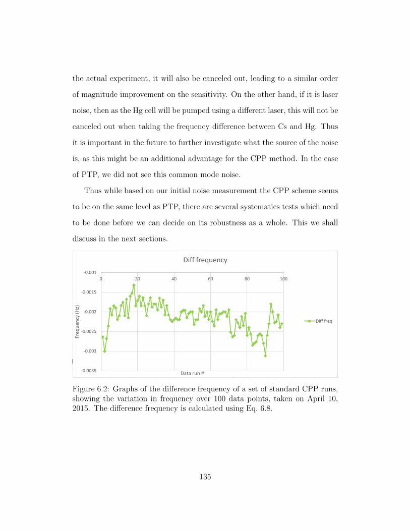
the actual experiment, it will also be canceled out, leading to a similar order
of magnitude improvement on the sensitivity. On the other hand, if it is laser
noise, then as the Hg cell will be pumped using a different laser, this will not be
canceled out when taking the frequency difference between Cs and Hg. Thus
it is important in the future to further investigate what the source of the noise
is, as this might be an additional advantage for the CPP method. In the case
of PTP, we did not see this common mode noise.
Thus while based on our initial noise measurement the CPP scheme seems
to be on the same level as PTP, there are several systematics tests which need
to be done before we can decide on its robustness as a whole. This we shall
discuss in the next sections.
20 40 60 80 100 120
Bot phase
-0.0035
-0.003
-0.0025
-0.002
-0.0015
-0.001
0 20 40 60 80 100
Freq
uen
cy (
Hz)
Data run #
Diff frequency
Diff freq
Figure 6.2: Graphs of the difference frequency of a set of standard CPP runs,showing the variation in frequency over 100 data points, taken on April 10,2015. The difference frequency is calculated using Eq. 6.8.
135
6.2 CPP Systematics Testing: Overview
The main systematics tests we will run on the CPP scheme will be similar to
PTP, in that we will vary the pump intensity, pump frequency, probe intensity,
and probe frequency. We will see if there are any stable operating regions that
give a frequency shift of less than the ultimate sensitivity goal of 32 µHz.
CPP differs from PTP, however, in that in addition to these, we have to pay
attention to the angle between the pump and probe lasers. This is because even
a slight misalignment will cause a phase shift between the pump and probe,
which is the quantity we are measuring. This is the greatest risk for the CPP
method. Another risk is because the pump is always on, we expect varying
parameters on the pump will affect the measurement. We do not, however,
have to worry about the duration of the pump or any fitting algorithms.
For all of the following investigations, we use the same settings as when
doing the noise measurement of Sec. 6.1. We measured the sensitivity η of
the cells each time and always found them to be approximately equal to the
values in Eq. 6.3. The y-axis values of the graphs displayed were originally
phase measured in degrees, which we divided by the relevant η to result in units
of frequency (Hz) that we can compare with PTP values. We are concerned
with the variation in these frequency values, as the absolute value of the phase
or frequency is meaningless (as opposed to PTP, where the absolute value of
the measured frequency is really the Larmor frequency).
136
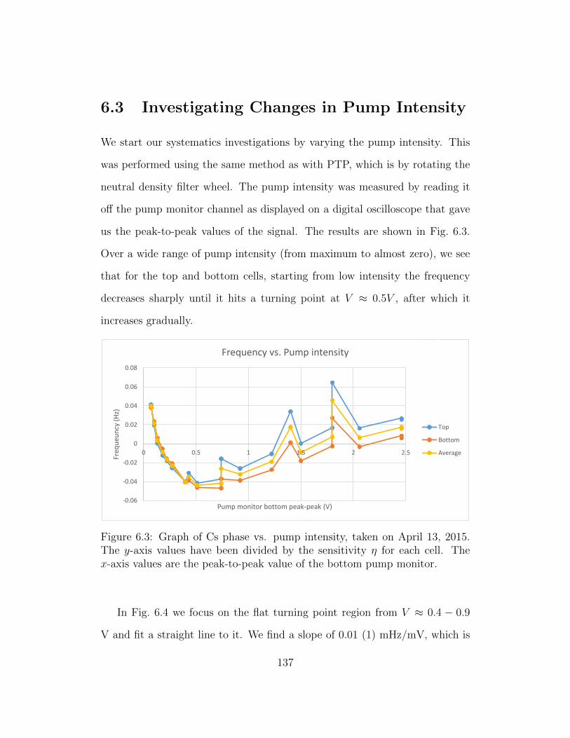
6.3 Investigating Changes in Pump Intensity
We start our systematics investigations by varying the pump intensity. This
was performed using the same method as with PTP, which is by rotating the
neutral density filter wheel. The pump intensity was measured by reading it
off the pump monitor channel as displayed on a digital oscilloscope that gave
us the peak-to-peak values of the signal. The results are shown in Fig. 6.3.
Over a wide range of pump intensity (from maximum to almost zero), we see
that for the top and bottom cells, starting from low intensity the frequency
decreases sharply until it hits a turning point at V ≈ 0.5V , after which it
increases gradually.
0.2
0.25
0.3
0.06227
0
0.1
0.2
0.3
0.4
0.5
0 0.5
-0.06
-0.04
-0.02
0
0.02
0.04
0.06
0.08
0 0.5 1 1.5 2 2.5
Freq
ueu
ncy
(H
z)
Pump monitor bottom peak-peak (V)
Frequency vs. Pump intensity
Top
Bottom
Average
Figure 6.3: Graph of Cs phase vs. pump intensity, taken on April 13, 2015.The y-axis values have been divided by the sensitivity η for each cell. Thex-axis values are the peak-to-peak value of the bottom pump monitor.
In Fig. 6.4 we focus on the flat turning point region from V ≈ 0.4 − 0.9
V and fit a straight line to it. We find a slope of 0.01 (1) mHz/mV, which is
137
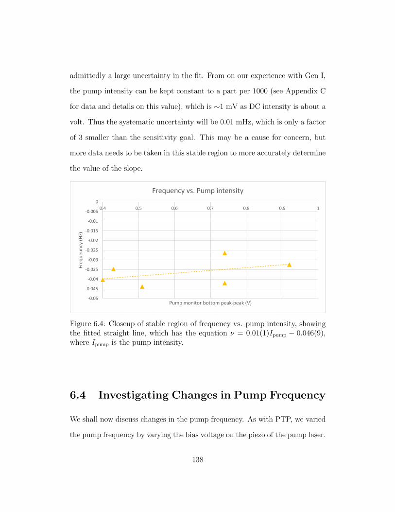
admittedly a large uncertainty in the fit. From on our experience with Gen I,
the pump intensity can be kept constant to a part per 1000 (see Appendix C
for data and details on this value), which is ∼1 mV as DC intensity is about a
volt. Thus the systematic uncertainty will be 0.01 mHz, which is only a factor
of 3 smaller than the sensitivity goal. This may be a cause for concern, but
more data needs to be taken in this stable region to more accurately determine
the value of the slope.
-0.005
0
0.4 0.5 0.6
Frequency vs. Pump intensity
-0.05
-0.045
-0.04
-0.035
-0.03
-0.025
-0.02
-0.015
-0.01
-0.005
0
0.4 0.5 0.6 0.7 0.8 0.9 1
Freq
ueu
ncy
(H
z)
Pump monitor bottom peak-peak (V)
Frequency vs. Pump intensity
Figure 6.4: Closeup of stable region of frequency vs. pump intensity, showingthe fitted straight line, which has the equation ν = 0.01(1)Ipump − 0.046(9),where Ipump is the pump intensity.
6.4 Investigating Changes in Pump Frequency
We shall now discuss changes in the pump frequency. As with PTP, we varied
the pump frequency by varying the bias voltage on the piezo of the pump laser.
138
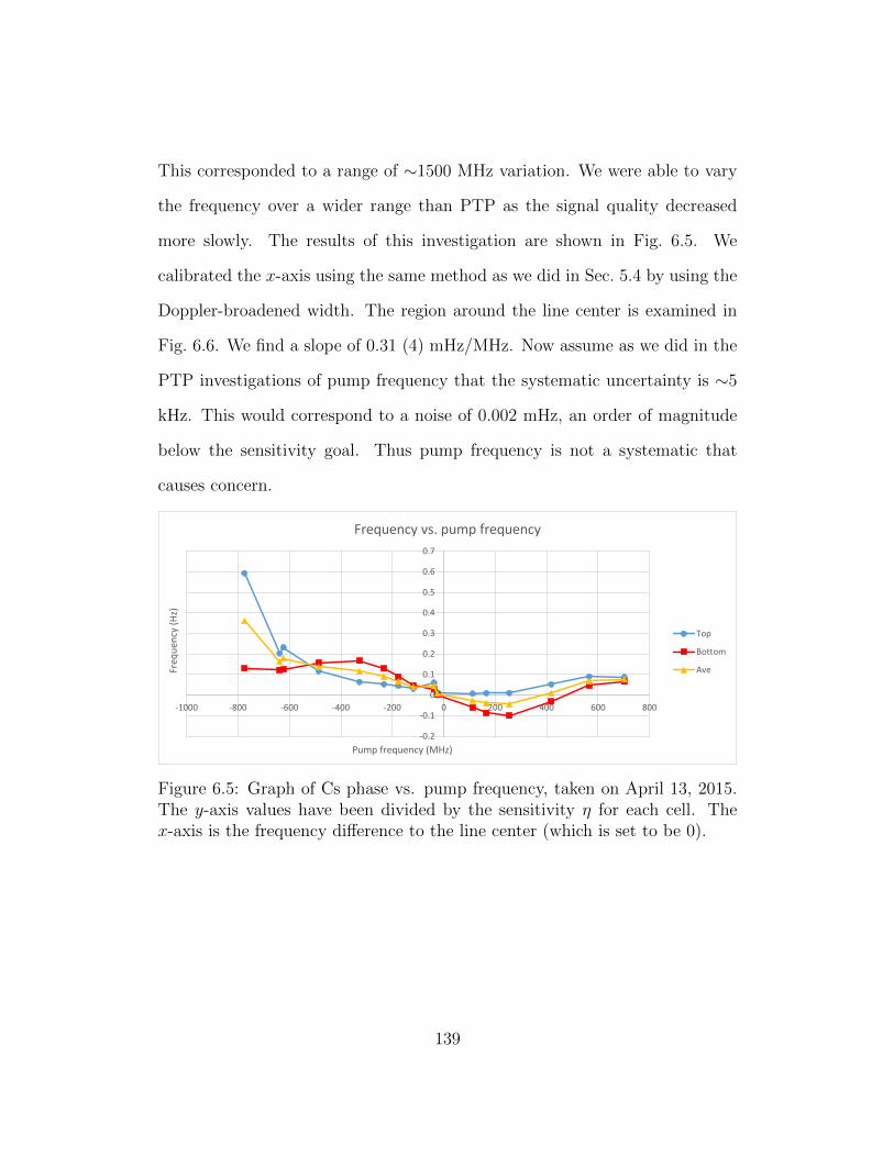
This corresponded to a range of ∼1500 MHz variation. We were able to vary
the frequency over a wider range than PTP as the signal quality decreased
more slowly. The results of this investigation are shown in Fig. 6.5. We
calibrated the x-axis using the same method as we did in Sec. 5.4 by using the
Doppler-broadened width. The region around the line center is examined in
Fig. 6.6. We find a slope of 0.31 (4) mHz/MHz. Now assume as we did in the
PTP investigations of pump frequency that the systematic uncertainty is ∼5
kHz. This would correspond to a noise of 0.002 mHz, an order of magnitude
below the sensitivity goal. Thus pump frequency is not a systematic that
causes concern.
-0.2
-0.1
0
0.1
0.2
0.3
0.4
0.5
0.6
0.7
-1000 -800 -600 -400 -200 0 200 400 600 800
Freq
uen
cy (
Hz)
Pump frequency (MHz)
Frequency vs. pump frequency
Top
Bottom
Ave
Figure 6.5: Graph of Cs phase vs. pump frequency, taken on April 13, 2015.The y-axis values have been divided by the sensitivity η for each cell. Thex-axis is the frequency difference to the line center (which is set to be 0).
139
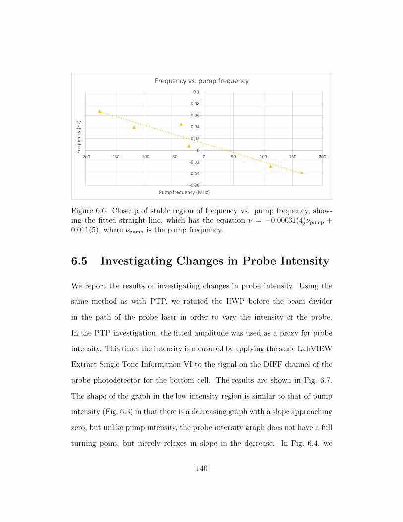
-0.06
-0.04
-0.02
0
0.02
0.04
0.06
0.08
0.1
-200 -150 -100 -50 0 50 100 150 200
Freq
uen
cy (
Hz)
Pump frequency (MHz)
Frequency vs. pump frequency
Figure 6.6: Closeup of stable region of frequency vs. pump frequency, show-ing the fitted straight line, which has the equation ν = −0.00031(4)νpump +0.011(5), where νpump is the pump frequency.
6.5 Investigating Changes in Probe Intensity
We report the results of investigating changes in probe intensity. Using the
same method as with PTP, we rotated the HWP before the beam divider
in the path of the probe laser in order to vary the intensity of the probe.
In the PTP investigation, the fitted amplitude was used as a proxy for probe
intensity. This time, the intensity is measured by applying the same LabVIEW
Extract Single Tone Information VI to the signal on the DIFF channel of the
probe photodetector for the bottom cell. The results are shown in Fig. 6.7.
The shape of the graph in the low intensity region is similar to that of pump
intensity (Fig. 6.3) in that there is a decreasing graph with a slope approaching
zero, but unlike pump intensity, the probe intensity graph does not have a full
turning point, but merely relaxes in slope in the decrease. In Fig. 6.4, we
140
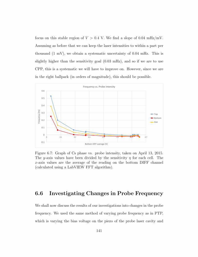
focus on this stable region of V > 0.4 V. We find a slope of 0.04 mHz/mV.
Assuming as before that we can keep the laser intensities to within a part per
thousand (1 mV), we obtain a systematic uncertainty of 0.04 mHz. This is
slightly higher than the sensitivity goal (0.03 mHz), and so if we are to use
CPP, this is a systematic we will have to improve on. However, since we are
in the right ballpark (in orders of magnitude), this should be possible.
-0.1
0
0.1
0.2
0.3
0.4
0.5
0.6
0 0.1 0.2 0.3 0.4 0.5 0.6 0.7
Freq
uen
cy (
Hz)
Bottom DIFF average (V)
Frequency vs. Probe intensity
Top
Bottom
Ave
Figure 6.7: Graph of Cs phase vs. probe intensity, taken on April 13, 2015.The y-axis values have been divided by the sensitivity η for each cell. Thex-axis values are the average of the reading on the bottom DIFF channel(calculated using a LabVIEW FFT algorithm).
6.6 Investigating Changes in Probe Frequency
We shall now discuss the results of our investigations into changes in the probe
frequency. We used the same method of varying probe frequency as in PTP,
which is varying the bias voltage on the piezo of the probe laser cavity and
141
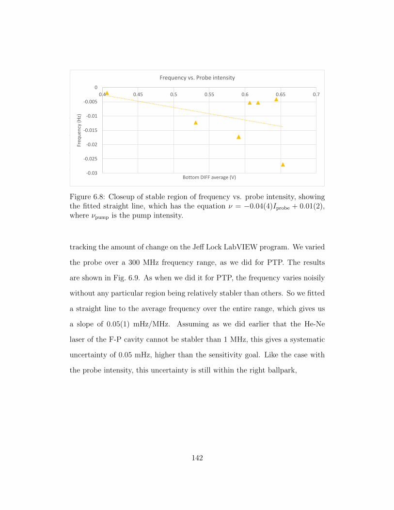
Frequency vs. Probe intensity
-0.03
-0.025
-0.02
-0.015
-0.01
-0.005
0
0.4 0.45 0.5 0.55 0.6 0.65 0.7
Freq
uen
cy (
Hz)
Bottom DIFF average (V)
Frequency vs. Probe intensity
Figure 6.8: Closeup of stable region of frequency vs. probe intensity, showingthe fitted straight line, which has the equation ν = −0.04(4)Iprobe + 0.01(2),where νpump is the pump intensity.
tracking the amount of change on the Jeff Lock LabVIEW program. We varied
the probe over a 300 MHz frequency range, as we did for PTP. The results
are shown in Fig. 6.9. As when we did it for PTP, the frequency varies noisily
without any particular region being relatively stabler than others. So we fitted
a straight line to the average frequency over the entire range, which gives us
a slope of 0.05(1) mHz/MHz. Assuming as we did earlier that the He-Ne
laser of the F-P cavity cannot be stabler than 1 MHz, this gives a systematic
uncertainty of 0.05 mHz, higher than the sensitivity goal. Like the case with
the probe intensity, this uncertainty is still within the right ballpark,
142
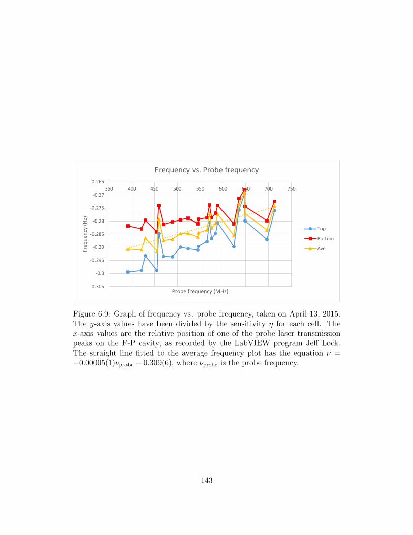
-0.305
-0.3
-0.295
-0.29
-0.285
-0.28
-0.275
-0.27
-0.265
350 400 450 500 550 600 650 700 750
Freq
uen
cy (
Hz)
Probe frequency (MHz)
Frequency vs. Probe frequency
Top
Bottom
Ave
Figure 6.9: Graph of frequency vs. probe frequency, taken on April 13, 2015.The y-axis values have been divided by the sensitivity η for each cell. Thex-axis values are the relative position of one of the probe laser transmissionpeaks on the F-P cavity, as recorded by the LabVIEW program Jeff Lock.The straight line fitted to the average frequency plot has the equation ν =−0.00005(1)νprobe − 0.309(6), where νprobe is the probe frequency.
143
6.7 Investigating Changes in Pump-Probe An-
gle
As has been mentioned in Sec. 6.2, for CPP it is important for the angle
between the pump and probe lasers, which are supposed to be orthogonal, to
be kept as constant as possible. There is a great risk of the lasers shifting as the
table rotates between the two positions. Based on our experience with Gen I,
we estimate that the laser beams will move with a total displacement standard
deviation of σtot = 0.4 millidegrees (see Appendix C for a fuller explanation on
how we derived this value, including some data plots from Gen I). Converting
this to frequency units using the cell sensitivities in Eq. 6.3, we get a variation
of
∆νtop = 0.02 mHz, (6.10)
∆νbot = 0.01 mHz, (6.11)
which is only slightly lower than the sensitivity goal. Thus if we want to use
CPP, we must make special efforts to keep this parameter under control.
6.8 Summary
Having investigated the phase response to the changing of various parameters
in the experiment using the CPP scheme, we summarize them in Tab. 6.1. As
we have seen, overall CPP performs worse than PTP in all systematics, which
is not surprising as in this scheme the pump is always on, so changes to it will
144
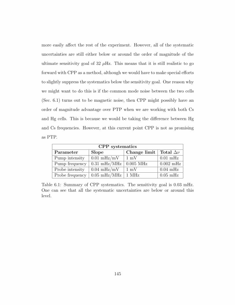
more easily affect the rest of the experiment. However, all of the systematic
uncertainties are still either below or around the order of magnitude of the
ultimate sensitivity goal of 32 µHz. This means that it is still realistic to go
forward with CPP as a method, although we would have to make special efforts
to slightly suppress the systematics below the sensitivity goal. One reason why
we might want to do this is if the common mode noise between the two cells
(Sec. 6.1) turns out to be magnetic noise, then CPP might possibly have an
order of magnitude advantage over PTP when we are working with both Cs
and Hg cells. This is because we would be taking the difference between Hg
and Cs frequencies. However, at this current point CPP is not as promising
as PTP.
CPP systematicsParameter Slope Change limit Total ∆νPump intensity 0.01 mHz/mV 1 mV 0.01 mHzPump frequency 0.31 mHz/MHz 0.005 MHz 0.002 mHzProbe intensity 0.04 mHz/mV 1 mV 0.04 mHzProbe frequency 0.05 mHz/MHz 1 MHz 0.05 mHz
Table 6.1: Summary of CPP systematics. The sensitivity goal is 0.03 mHz.One can see that all the systematic uncertainties are below or around thislevel.
145
Chapter 7
Conclusions and Future Outlook
We have finished describing the theoretical motivations of our experiment,
the physics behind it, and the physical details of the apparatus. We have
also reported the current results of our ongoing investigation into systematic
effects. In this chapter, we shall summarize all of these findings and also take
a brief look at the future plans for the Gen II experiment.
7.1 Summary of Findings
We have explored the systematic effects of changing pump intensity, pump
frequency, probe intensity, and probe frequency on the Larmore frequency
being measured on both the PTP and CPP schemes. We have also dealt with
some peculiar features of each scheme (the fitting process in PTP, and pump-
probe alignment in CPP). Tab. 7.1 summarizes the findings, comparing PTP
and CPP directly. PTP clearly has roughly an order of magnitude advantage in
the systematic uncertainties compared to CPP. As the statistical noise level of
146
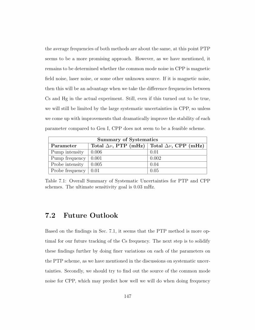
the average frequencies of both methods are about the same, at this point PTP
seems to be a more promising approach. However, as we have mentioned, it
remains to be determined whether the common mode noise in CPP is magnetic
field noise, laser noise, or some other unknown source. If it is magnetic noise,
then this will be an advantage when we take the difference frequencies between
Cs and Hg in the actual experiment. Still, even if this turned out to be true,
we will still be limited by the large systematic uncertainties in CPP, so unless
we come up with improvements that dramatically improve the stability of each
parameter compared to Gen I, CPP does not seem to be a feasible scheme.
Summary of SystematicsParameter Total ∆ν, PTP (mHz) Total ∆ν, CPP (mHz)Pump intensity 0.006 0.01Pump frequency 0.001 0.002Probe intensity 0.005 0.04Probe frequency 0.01 0.05
Table 7.1: Overall Summary of Systematic Uncertainties for PTP and CPPschemes. The ultimate sensitivity goal is 0.03 mHz.
7.2 Future Outlook
Based on the findings in Sec. 7.1, it seems that the PTP method is more op-
timal for our future tracking of the Cs frequency. The next step is to solidify
these findings further by doing finer variations on each of the parameters on
the PTP scheme, as we have mentioned in the discussions on systematic uncer-
tainties. Secondly, we should try to find out the source of the common mode
noise for CPP, which may predict how well we will do when doing frequency
147
subtraction with the Hg cell.
Next, we should investigate our fitting process for PTP more thoroughly.
Even if we cannot make the fitting algorithm give a stable result when varying
some of its parameters, we should decide on what settings to use and stick
to them for the rest of the experiment. Additionally, we might also consider
replacing the Pockels cell with an Acousto-optic Modulator (AOM) that will
extinguish the pump light better during the optical probing stage of PTP. As
we have briefly mentioned in Sec. 5.7, this is another possibility for why PTP
is currently vulnerable to changes in pumping parameters.
Another task to be done in the near future is to open up the cans and
reverse the top and bottom cells to see if their lifetimes remain the same, in
order to resolve the mystery reported in Sec. 3.2.3, where the lifetime of the
“short stem” cell dropped by a factor of 2 from ∼90 ms to the current value
of 43 ms.
After completing all of these investigations on cesium, we have to do similar
experiments on the mercury cells. We anticipate receiving the new Hg cells
in the next few months. For Hg, we only have one laser, and it would be
cost-prohibitive to purchase another one, so the CPP geometry is out of the
question. The only way to track the Hg Larmor frequency would be to pump
and probe using the same laser, using a scheme similar to PTP. The laser would
first pump for a set time, modulated at the Larmor frequency of Hg. Then it
would immediately be shifted 3 GHz away from resonance for probing. With
the Cs lasers, we normally have to manually adjust the laser current when
changing the bias voltage to detune from resonance. The Hg ultraviolet laser,
148
however, has a feature in its electronics that should be able to automatically
adjust the laser when the bias voltage increases by a large amount.
We tried using this single laser PTP scheme in the early stages of the
thesis (May-June 2014) with little success as the lifetimes of the Cs cells are
so short (tens of milliseconds). Thus there was not enough time to detune the
laser several GHz off resonance for probing, and we were stuck at probing at
resonance, which was unsuccessful and led to adoption of the current two-laser
geometry. With Hg, however, a typical lifetime is ∼4 s. Hopefully, this makes
such a scheme much easier to realize.
After doing systematics testing on the Hg, we would start designing and
building the components needed to fit our new Gen II geometry on the rotating
table apparatus. While we will probably be able to reuse the rotating table and
magnetic shields from Gen I, we will still have to think about how to mount
the probe detectors and the cells, as well as how to monitor the pump. Only
then would we finally be able to take data for Gen II, apply our geophysical
method and obtain newly improved bounds for LRSSIs.
149
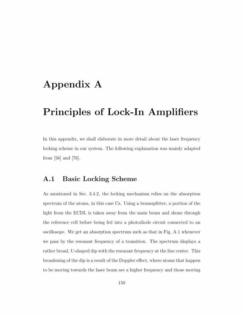
Appendix A
Principles of Lock-In Amplifiers
In this appendix, we shall elaborate in more detail about the laser frequency
locking scheme in our system. The following explanation was mainly adapted
from [56] and [76].
A.1 Basic Locking Scheme
As mentioned in Sec. 3.4.2, the locking mechanism relies on the absorption
spectrum of the atoms, in this case Cs. Using a beamsplitter, a portion of the
light from the ECDL is taken away from the main beam and shone through
the reference cell before being fed into a photodiode circuit connected to an
oscillosope. We get an absorption spectrum such as that in Fig. A.1 whenever
we pass by the resonant frequency of a transition. The spectrum displays a
rather broad, U-shaped dip with the resonant frequency at the line center. This
broadening of the dip is a result of the Doppler effect, where atoms that happen
to be moving towards the laser beam see a higher frequency and those moving
150
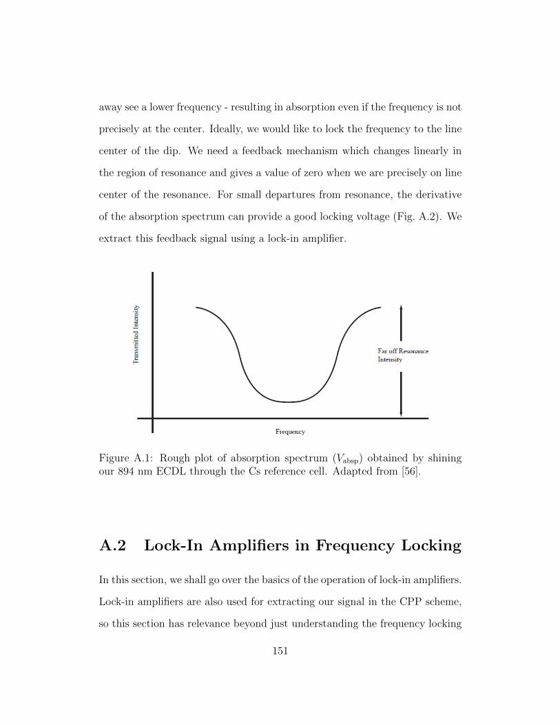
away see a lower frequency - resulting in absorption even if the frequency is not
precisely at the center. Ideally, we would like to lock the frequency to the line
center of the dip. We need a feedback mechanism which changes linearly in
the region of resonance and gives a value of zero when we are precisely on line
center of the resonance. For small departures from resonance, the derivative
of the absorption spectrum can provide a good locking voltage (Fig. A.2). We
extract this feedback signal using a lock-in amplifier.
Figure A.1: Rough plot of absorption spectrum (Vabsp) obtained by shiningour 894 nm ECDL through the Cs reference cell. Adapted from [56].
A.2 Lock-In Amplifiers in Frequency Locking
In this section, we shall go over the basics of the operation of lock-in amplifiers.
Lock-in amplifiers are also used for extracting our signal in the CPP scheme,
so this section has relevance beyond just understanding the frequency locking
151
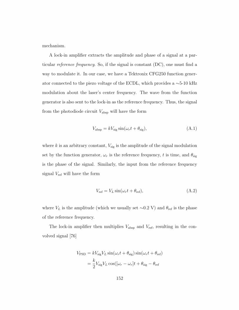
mechanism.
A lock-in amplifier extracts the amplitude and phase of a signal at a par-
ticular reference frequency. So, if the signal is constant (DC), one must find a
way to modulate it. In our case, we have a Tektronix CFG250 function gener-
ator connected to the piezo voltage of the ECDL, which provides a ∼5-10 kHz
modulation about the laser’s center frequency. The wave from the function
generator is also sent to the lock-in as the reference frequency. Thus, the signal
from the photodiode circuit Vabsp will have the form
Vabsp = kVsig sin(ωrt+ θsig), (A.1)
where k is an arbitrary constant, Vsig is the amplitude of the signal modulation
set by the function generator, ωr is the reference frequency, t is time, and θsig
is the phase of the signal. Similarly, the input from the reference frequency
signal Vref will have the form
Vref = VL sin(ωrt+ θref), (A.2)
where VL is the amplitude (which we usually set ∼0.2 V) and θref is the phase
of the reference frequency.
The lock-in amplifier then multiplies Vabsp and Vref, resulting in the con-
volved signal [76]
VPSD = kVsigVL sin(ωrt+ θsig) sin(ωrt+ θref)
=k
2VsigVL cos([ωr − ωr]t+ θsig − θref
152
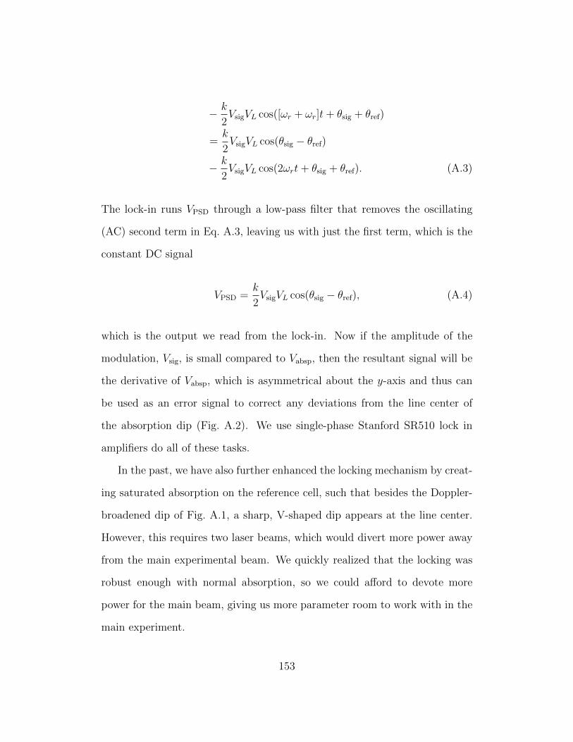
− k
2VsigVL cos([ωr + ωr]t+ θsig + θref)
=k
2VsigVL cos(θsig − θref)
− k
2VsigVL cos(2ωrt+ θsig + θref). (A.3)
The lock-in runs VPSD through a low-pass filter that removes the oscillating
(AC) second term in Eq. A.3, leaving us with just the first term, which is the
constant DC signal
VPSD =k
2VsigVL cos(θsig − θref), (A.4)
which is the output we read from the lock-in. Now if the amplitude of the
modulation, Vsig, is small compared to Vabsp, then the resultant signal will be
the derivative of Vabsp, which is asymmetrical about the y-axis and thus can
be used as an error signal to correct any deviations from the line center of
the absorption dip (Fig. A.2). We use single-phase Stanford SR510 lock in
amplifiers do all of these tasks.
In the past, we have also further enhanced the locking mechanism by creat-
ing saturated absorption on the reference cell, such that besides the Doppler-
broadened dip of Fig. A.1, a sharp, V-shaped dip appears at the line center.
However, this requires two laser beams, which would divert more power away
from the main experimental beam. We quickly realized that the locking was
robust enough with normal absorption, so we could afford to devote more
power for the main beam, giving us more parameter room to work with in the
main experiment.
153
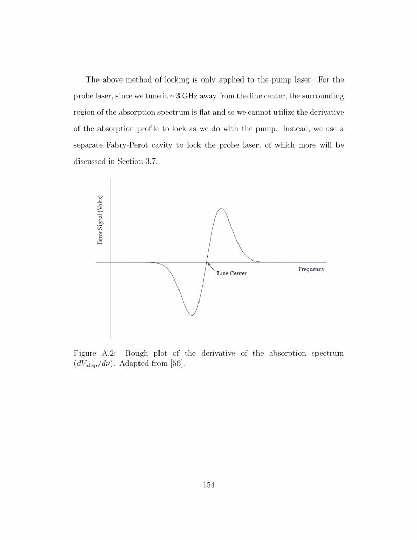
The above method of locking is only applied to the pump laser. For the
probe laser, since we tune it∼3 GHz away from the line center, the surrounding
region of the absorption spectrum is flat and so we cannot utilize the derivative
of the absorption profile to lock as we do with the pump. Instead, we use a
separate Fabry-Perot cavity to lock the probe laser, of which more will be
discussed in Section 3.7.
Figure A.2: Rough plot of the derivative of the absorption spectrum(dVabsp/dν). Adapted from [56].
154
Appendix B
Basic Running Procedure
In this appendix we shall discuss in more detail the general settings we nor-
mally use when operating our apparatus.
The first thing we do daily is to turn on both the pump and probe lasers,
and adjust the current for each so that it is at the setting that corresponds
with roughly where the relevant atomic transitions are: for the pump, it is the
62S1/2(F = 3) → 62P1/2(F ′ = 4) transition, whereas for the probe it is the
62S1/2(F = 4)→ 62P1/2(F ′ = 3). Using the reference cells, we then do adjust
the bias voltage on the piezos using a simple electronics box so that the lasers
are on the line center of the absorption profile. We let the lasers stabilize for
an hour or so.
We then apply a small amplitude, ∼400 Hz modulation to the pump laser
using the Tektronix CFG250 function generator. The lock function is then
turned on, and the pump is locked. For the probe, we take note of the starting
position of an F-P transmission peak of the laser on the Jeff Lock program.
155
We then start increasing the bias voltage on the piezo while observing the
movement of the transmission peaks on Jeff Lock. We keep increasing the
voltage until we have seen 6 successive transmission peaks pass through. As
we do this, we have to sometimes decrease the current to prevent the laser
from going multi-mode.1 Now, as the FSR of the F-P is ∼500 Hz, this means
that we have effectively tuned roughly 3 GHz away from line resonance center.
The figure of 3 GHz was chosen because in our early investigations, tuning
further away only further decreased the signal without increasing the lifetime.
At the current stage of the experiment, it is not important that we tune
precisely to the same position every day, because small deviations in the probe
frequency do not affect the system’s behavior in a significant way, as long as we
are within a few hundred MHz from the 3 GHz detuning.2 Another important
question is why we increase the voltage, effectively tuning it 3 GHz to the
left of the Cs absorption profile of Fig. 2.4, such that the laser is somewhere
between the F = 3 → F = 3 and F = 4 → F = 4 transitions. The answer is
that we did try tuning the other way when doing the lifetime measurements,
and found that for some reason the signal-to-noise ratio was slightly better
when tuning to the left.
Lastly, we have also briefly investigated different combinations of Cs transi-
tions on the pump and probe. We tried all 16 different combinations using the
1If we do not do this, then the laser will eventually mode hop back to the originalfrequency.
2As we discuss in Chs. 5 and 6, the actual frequency can indeed change a little bit asthe probe frequency deviates. So it is important to keep the probe frequency stable withina single series of runs that are meant to be used to analyze a single property of the system.But it is not as important to keep it stable over several series of runs that aim to investigatedifferent things.
156

4 hyperfine levels. At that point, we had not started tuning the probe away
from resonance, and so the probe was also tuned at or near the line center.
In this configuration, only a few combinations worked at all; the results were
much better when the two lasers were at different transitions. It was then
determined that the current setup of pump at F = 3 → F ′ = 4 and probe at
F = 4 → F ′ = 3 gave the best results. As we now regularly tune the probe
3 GHz away instead of putting it at line center, the initial transition of the
probe does not matter as much.
After locking the pump laser, we turn on the He-Ne laser, wait about an
hour for it to warm up and stabilize, then activate its locking function that
locks the ratio of axial and transverse modes of polarizations, effectively locking
the cavity length. Jeff Lock is thus ready to lock the probe laser. In reality,
the probe laser is quite stable as is without being locked, especially within the
time scales we are investigating at (only 30 minutes at most). Thus often we
do not bother to activate Jeff Lock’s locking function at all.
Once the locking is done, we turn on the signal amplifier that converts
modulation of a few volts to the several hundred volts needed for the Pockels
Cell. We also turn on the high voltage power supply from which it draws
power, setting it to a maximum of 350 V. The power supply for the magnetic
field coils are also turned on to the standard voltage of Vbase = 9.74 V. We
turn on the power supply for the probe photodetectors. We are then ready to
operate within one of the two possible data collection schemes: PTP or CPP.
These schemes are described in Ch. 4.
157
Appendix C
Beam Movement and Laser
Intensity Variation in Gen I
In this Appendix, we will explain further our method of estimating the amount
of variation in beam movement and laser intensity in Gen I, which are useful
as rough guides on the future behavior of Gen II.
C.1 Beam Movement
First, we shall discuss our method to estimate how much the laser beam can
move as we switch back and forth between the two table positions. In the
Gen I apparatus, a fiber bundle was positioned at the top of the cans point-
ing downwards (see Fig. 2.9) to collect the light from the laser after passing
through the vapor cells. The fiber bundle was divided into 4 quadrants which
went into 4 separate photodiodes, numbered in clockwise order DC1 to DC4.
158
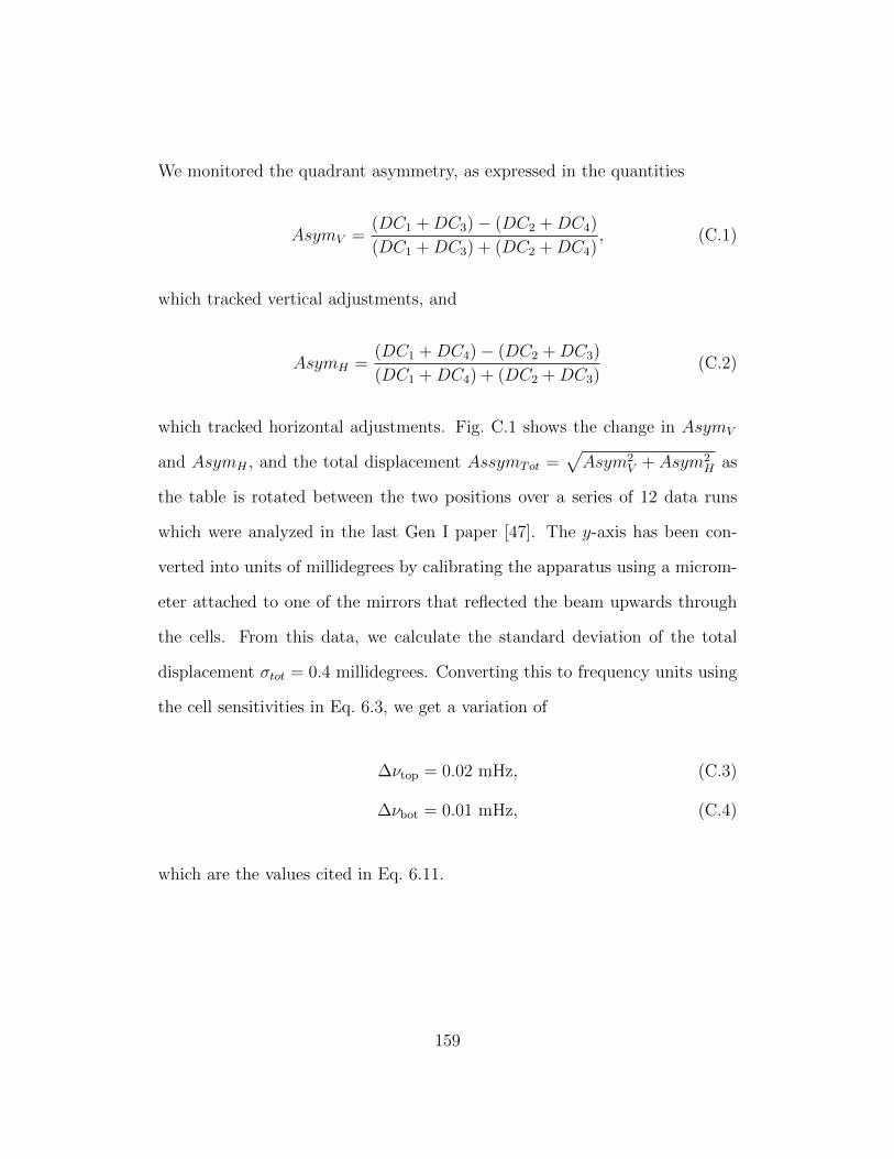
We monitored the quadrant asymmetry, as expressed in the quantities
AsymV =(DC1 +DC3)− (DC2 +DC4)
(DC1 +DC3) + (DC2 +DC4), (C.1)
which tracked vertical adjustments, and
AsymH =(DC1 +DC4)− (DC2 +DC3)
(DC1 +DC4) + (DC2 +DC3)(C.2)
which tracked horizontal adjustments. Fig. C.1 shows the change in AsymV
and AsymH , and the total displacement AssymTot =√Asym2
V + Asym2H as
the table is rotated between the two positions over a series of 12 data runs
which were analyzed in the last Gen I paper [47]. The y-axis has been con-
verted into units of millidegrees by calibrating the apparatus using a microm-
eter attached to one of the mirrors that reflected the beam upwards through
the cells. From this data, we calculate the standard deviation of the total
displacement σtot = 0.4 millidegrees. Converting this to frequency units using
the cell sensitivities in Eq. 6.3, we get a variation of
∆νtop = 0.02 mHz, (C.3)
∆νbot = 0.01 mHz, (C.4)
which are the values cited in Eq. 6.11.
159
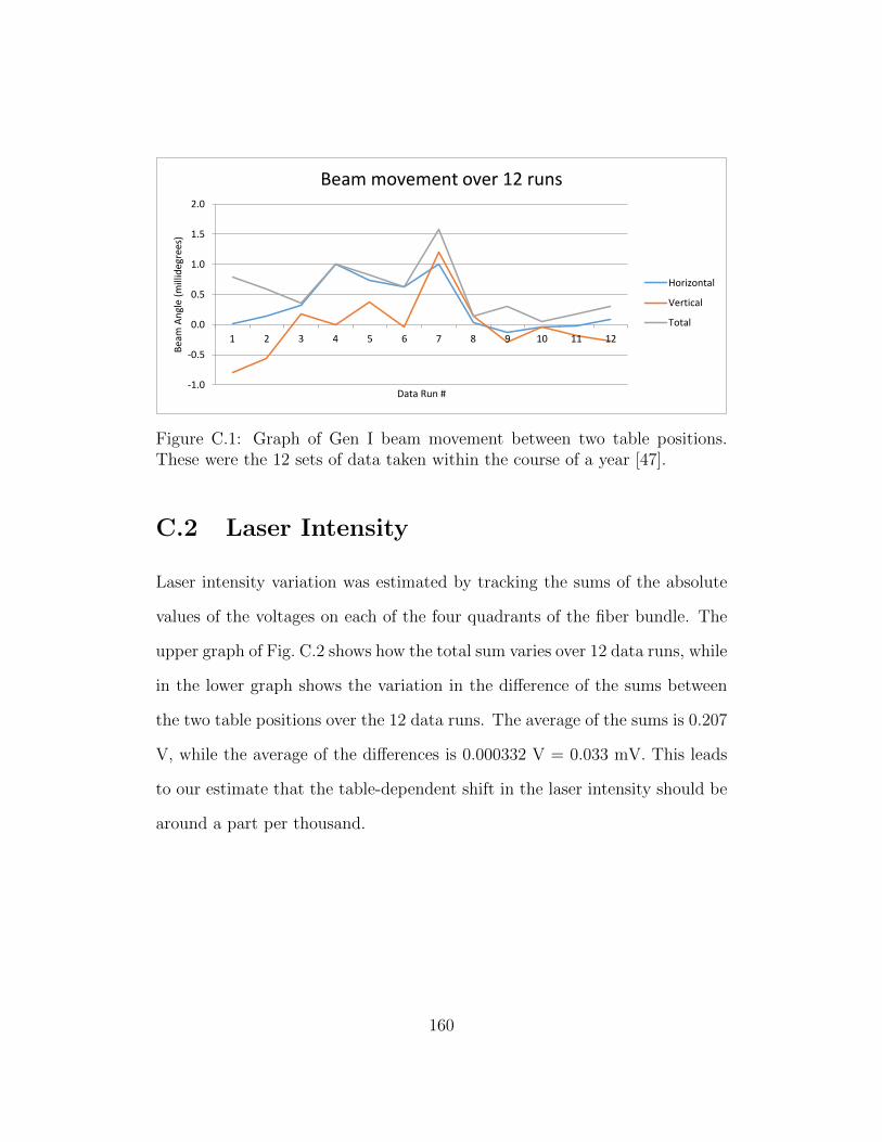
-1.0
-0.5
0.0
0.5
1.0
1.5
2.0
1 2 3 4 5 6 7 8 9 10 11 12
Bea
m A
ngl
e (m
illid
egre
es)
Data Run #
Beam movement over 12 runs
Horizontal
Vertical
Total
Figure C.1: Graph of Gen I beam movement between two table positions.These were the 12 sets of data taken within the course of a year [47].
C.2 Laser Intensity
Laser intensity variation was estimated by tracking the sums of the absolute
values of the voltages on each of the four quadrants of the fiber bundle. The
upper graph of Fig. C.2 shows how the total sum varies over 12 data runs, while
in the lower graph shows the variation in the difference of the sums between
the two table positions over the 12 data runs. The average of the sums is 0.207
V, while the average of the differences is 0.000332 V = 0.033 mV. This leads
to our estimate that the table-dependent shift in the laser intensity should be
around a part per thousand.
160
0
0.05
0.1
0.15
0.2
0.25
0.3
0.35
2 3 4 5 6 7 8 9 10 11 12
Inte
nsi
ty (
V)
Data run #
Total intensity over 12 runs
Beam movement over 12 runs
0
0.0001
0.0002
0.0003
0.0004
0.0005
0.0006
0.0007
0.0008
0.0009
2 3 4 5 6 7 8 9 10 11 12
Inte
nsi
ty (
V)
Data run #
Difference in total intensity between table positions over 12 runs
Figure C.2: Graph of Gen I beam movement between two table positions.These were the 12 sets of data taken within the course of a year [47].
161

Bibliography
[1] Hunter, L., Gordon, J., Peck, S., Ang, D. & Lin, J.-F. Using the earth as
a polarized electron source to search for long-range spin-spin interactions.
Science 339, 928–932 (2013).
[2] Hunter, L. & Ang, D. Using geoelectrons to search for velocity-dependent
spin-spin interactions. Phys. Rev. Lett. 112, 091803 (2014).
[3] Griffiths, D. Introduction to Electrodynamics. Always learning (Pearson,
2013).
[4] Einstein, A. Zur Elektrodynamik bewegter Korper. Annalen der Physik
322, 891–921 (1905).
[5] Einstein, A. Uber einen die Erzeugung und Verwandlung des Lichtes
betreffenden heuristischen Gesichtspunkt. Annalen der Physik 322, 132–
148 (1905).
[6] Einstein, A. Uber den Einfluß der Schwerkraft auf die Ausbreitung des
Lichtes. Annalen der Physik 340, 898–908 (1911).
[7] Kragh, H. Quantum Generations: A History of Physics in the Twentieth
162
Century. History and philosophy of science (Princeton University Press,
2002).
[8] Hanneke, D., Fogwell, S. & Gabrielse, G. New measurement of the elec-
tron magnetic moment and the fine structure constant. Phys. Rev. Lett.
100, 120801 (2008).
[9] Glashow, S. L. Partial-symmetries of weak interactions. Nuclear Physics
A 22, 579–588 (1961).
[10] Weinberg, S. A Model of Leptons. Phys. Rev. Lett. 19, 1264–1266 (1967).
[11] Griffiths, D. Introduction to Elementary Particles. Physics textbook
(Wiley, 2008).
[12] Aubert, J.-J. et al. Experimental observation of a heavy particle j. Phys-
ical Review Letters 33, 1404 (1974).
[13] Augustin, J.-E. et al. Discovery of a narrow resonance in e+ e-
annihilation. Physical Review Letters 33, 1406 (1974).
[14] Fritzsch, H. The History of QCD (2012). [Online at http:
//cerncourier.com/cws/article/cern/50796; accessed 26 January
2015].
[15] Chatrchyan, S. et al. Observation of a new boson at a mass of 125 GeV
with the CMS experiment at the LHC. Physics Letters B 716, 30–61
(2012). 1207.7235.
163
[16] Aad, G. et al. Observation of a new particle in the search for the Standard
Model Higgs boson with the ATLAS detector at the LHC. Physics Letters
B 716, 1–29 (2012). 1207.7214.
[17] Zwiebach, B. A First Course in String Theory (Cambridge University
Press, 2009).
[18] Lee, T. D. & Yang, C. N. Question of parity conservation in weak inter-
actions. Phys. Rev. 104, 254–258 (1956).
[19] Wu, C. S., Ambler, E., Hayward, R. W., Hoppes, D. D. & Hudson, R. P.
Experimental test of parity conservation in beta decay. Phys. Rev. 105,
1413–1415 (1957).
[20] Christenson, J. H., Cronin, J. W., Fitch, V. L. & Turlay, R. Evidence for
the 2π decay of the k02 meson. Phys. Rev. Lett. 13, 138–140 (1964).
[21] Jaeckel, J. & Ringwald, A. The Low-Energy Frontier of Particle Physics.
In Holstein, BR and Haxton, WC and Jawahery, A (ed.) ANNUAL RE-
VIEW OF NUCLEAR AND PARTICLE SCIENCE, VOL 60, vol. 60
of Annual Review of Nuclear and Particle Science, 405–437 (ANNUAL
REVIEWS, 2010).
[22] Amsler, C. et al. Review of particle physics. Physics Letters B 667, 1 –
6 (2008). Review of Particle Physics.
[23] Peccei, R. D. & Quinn, H. R. CP conservation in the presence of pseu-
doparticles. Phys. Rev. Lett. 38, 1440–1443 (1977).
164
[24] Moody, J. E. & Wilczek, F. New macroscopic forces? Phys. Rev. D 30,
130–138 (1984).
[25] Youdin, A. N., Krause, D., Jr., Jagannathan, K., Hunter, L. R. & Lam-
oreaux, S. K. Limits on spin-mass couplings within the axion window.
Phys. Rev. Lett. 77, 2170–2173 (1996).
[26] Ni, W.-T., Pan, S.-s., Yeh, H.-C., Hou, L.-S. & Wan, J. Search for an
axionlike spin coupling using a paramagnetic salt with a dc squid. Phys.
Rev. Lett. 82, 2439–2442 (1999).
[27] Phillips, D. F. et al. Limit on lorentz and CPT violation of the proton
using a hydrogen maser. Phys. Rev. D 63, 111101 (2001).
[28] Nakamura, K. & Group, P. D. Review of particle physics. Journal of
Physics G: Nuclear and Particle Physics 37, 075021 (2010).
[29] Dobrescu, B. A. & Mocioiu, I. Spin-dependent macroscopic forces from
new particle exchange. Journal of High Energy Physics 2006, 005 (2006).
[30] Essig, R. et al. Working Group Report: New Light Weakly Coupled
Particles (2013). 1311.0029.
[31] Davoudiasl, H., Lee, H.-S. & Marciano, W. J. ’Dark’ Z implications for
Parity Violation, Rare Meson Decays, and Higgs Physics. Phys.Rev. D85,
115019 (2012). 1203.2947.
[32] Bjorken, J. D. et al. Search for neutral metastable penetrating particles
produced in the slac beam dump. Phys. Rev. D 38, 3375–3386 (1988).
165
[33] Andreas, S., Niebuhr, C. & Ringwald, A. New limits on hidden photons
from past electron beam dumps. Phys. Rev. D 86, 095019 (2012).
[34] Dobrescu, B. A. Massless gauge bosons other than the photon. Phys.
Rev. Lett. 94, 151802 (2005).
[35] Georgi, H. Unparticle physics. Phys. Rev. Lett. 98, 221601 (2007).
[36] Liao, Y. & Liu, J.-Y. Long-range electron spin-spin interactions from
unparticle exchange. Physical review letters 99, 191804 (2007).
[37] Neville, D. E. Experimental bounds on the coupling of massless spin-1
torsion. Phys. Rev. D 25, 573–576 (1982).
[38] Hewett, J. L. & Rizzo, T. G. Low-energy phenomenology of superstring-
inspired E6 models. Physics Reports 183, 193 – 381 (1989).
[39] Wang, L. & Han, X.-F. Rare z-decay into light pseudoscalar bosons in
the simplest little higgs model. Nuclear Physics B 853, 625–634 (2011).
[40] Hill, C. T. Topcolor assisted technicolor. Physics Letters B 345, 483 –
489 (1995).
[41] Rizzo, T. G. Z-prime bosons and Kaluza-Klein excitations at muon col-
liders. AIP Conf.Proc. 542, 152–159 (2000). hep-ph/0001140.
[42] Heckel, B. R., Adelberger, E. G., Gundlach, J. H., Harris, M. G. & Swan-
son, H. E. Torsion balance test of spin coupled forces. In Quantum Grav-
ity, Generalized Theory of Gravitation, and Superstring Theory-Based
Unification, 153–160 (Springer, 2002).
166
[43] Vasilakis, G., Brown, J. M., Kornack, T. W. & Romalis, M. V. Lim-
its on new long range nuclear spin-dependent forces set with a K-3He
comagnetometer. Phys. Rev. Lett. 103, 261801 (2009).
[44] Hou, L.-S., Ni, W.-T. & Li, Y.-C. M. Test of cosmic spatial isotropy for
polarized electrons using a rotatable torsion balance. Phys. Rev. Lett. 90,
201101 (2003).
[45] Brown, J. M., Smullin, S. J., Kornack, T. W. & Romalis, M. V. New
limit on lorentz- and cpt-violating neutron spin interactions. Phys. Rev.
Lett. 105, 151604 (2010).
[46] Heckel, B. R. et al. Preferred-frame and cp-violation tests with polarized
electrons. Phys. Rev. D 78, 092006 (2008).
[47] Peck, S. et al. Limits on local lorentz invariance in mercury and cesium.
Physical Review A 86, 012109 (2012).
[48] Venema, B. J., Majumder, P. K., Lamoreaux, S. K., Heckel, B. R. &
Fortson, E. N. Search for a coupling of the earth’s gravitational field to
nuclear spins in atomic mercury. Phys. Rev. Lett. 68, 135–138 (1992).
[49] Maus, S. et al. The us/uk world magnetic model for 2010-2015 (2010).
[50] Poirier, J. Introduction to the Physics of the Earth’s Interior (Cambridge
University Press, 2000).
[51] Alfe, D. & Gillan, M. J. First-principles calculation of transport coeffi-
cients. Phys. Rev. Lett. 81, 5161–5164 (1998).
167
[52] Jackson Kimball, D. F., Boyd, A. & Budker, D. Constraints on anomalous
spin-spin interactions from spin-exchange collisions. Phys. Rev. A 82,
062714 (2010).
[53] Kimball, D. F. J. et al. A dual-isotope rubidium comagnetometer to
search for anomalous long-range spin-mass (spin-gravity) couplings of the
proton. Annalen der Physik 525, 514–528 (2013).
[54] Brown, J. M., Smullin, S. J., Kornack, T. W. & Romalis, M. V. New
limit on lorentz- and cpt-violating neutron spin interactions. Phys. Rev.
Lett. 105, 151604 (2010).
[55] Harris, R. Modern Physics (Pearson/Addison Wesley, 2008).
[56] Stein, D. A Test of Special Relativity - Pushing down the Limits on a
Possible Violation of Local Lorentz Invariance. Bachelor’s thesis, Amherst
College, Amherst, MA (2006).
[57] Steck, D. A. Cesium d line data. Los Alamos National Laboratory (un-
published) 124 (2003).
[58] Happer, W. Optical pumping. Rev. Mod. Phys. 44, 169–249 (1972).
[59] Sagle, J., Namiotka, R. & Huennekens, J. Measurement and modelling of
intensity dependent absorption and transit relaxation on the cesium line.
Journal of Physics B: Atomic, Molecular and Optical Physics 29, 2629
(1996).
168
[60] Bell, W. E. & Bloom, A. L. Optical detection of magnetic resonance in
alkali metal vapor. Phys. Rev. 107, 1559–1565 (1957).
[61] Budker, D. & Kimball, D. Optical Magnetometry. Optical Magnetometry
(Cambridge University Press, 2013).
[62] Jackson, J. Classical Electrodynamics (Wiley, 1998).
[63] Hummon, M. The Search for Violations of Local Lorentz Invariance Using
Hg and Cs Magnetometers. Bachelor’s thesis, Amherst College, Amherst,
MA (2002).
[64] Foss, A. Measuring a Violation of Local Lorentz Invariance. Bachelor’s
thesis, Amherst College, Amherst, MA (2003).
[65] Orbaker, D. Spinning the Spins: Constructing a Rotating Apparatus to
Set New Limits on Local Lorentz Invariance. Bachelor’s thesis, Amherst
College, Amherst, MA (2004).
[66] Kim, D.-K. A Search for Local Lorentz Violation. Bachelor’s thesis,
Amherst College, Amherst, MA (2008).
[67] Heckel, B. R. et al. Preferred-frame and cp-violation tests with polarized
electrons. Phys. Rev. D 78, 092006 (2008).
[68] Mathur, B., Tang, H. & Happer, W. Light shifts in the alkali atoms.
Physical Review 171, 11 (1968).
[69] Happer, W. & Mathur, B. S. Effective operator formalism in optical
pumping. Phys. Rev. 163, 12–25 (1967).
169
[70] Budker, D., Kimball, D. & DeMille, D. Atomic Physics: An Exploration
Through Problems and Solutions (Oxford University Press, 2004).
[71] Murthy, S. A., Krause, D., Li, Z. L. & Hunter, L. R. New limits on the
electron electric dipole moment from cesium. Phys. Rev. Lett. 63, 965–968
(1989).
[72] Balabas, M. V., Karaulanov, T., Ledbetter, M. P. & Budker, D. Polarized
alkali-metal vapor with minute-long transverse spin-relaxation time. Phys.
Rev. Lett. 105, 070801 (2010).
[73] Teng, C. Frequency Control and Stabilization of a Laser System. Bache-
lor’s thesis, Amherst College, Amherst, MA (2013).
[74] Vaughan, M. The Fabry-Perot Interferometer: History, Theory, Practice
and Applications. Series in Optics and Optoelectronics (Taylor & Francis,
1989).
[75] Araki, M. Pid control. Control systems, robotics and automation 2, 1–23
(2002).
[76] Stanford Research Systems. About Lock-In Amplifiers: Application Note
#3.
170
Recommended