© 2011 ANSYS, Inc. March 15, 20121
Improving Your Structural Mechanics Simulations with Release 14.0
Mai Doan [email protected]
Sreekanth Akarapu [email protected]
© 2011 ANSYS, Inc. March 15, 20122
Structural Mechanics Themes
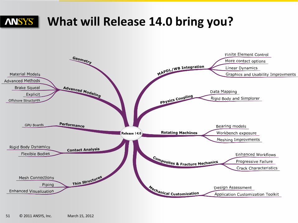
MAPDL/WB Integration
Physics coupling
Rotating machines
Composites & Fracture Mechanics
Application Customization
Advanced Modeling
Performance
Thin structures modeling
Contact analysis
© 2011 ANSYS, Inc. March 15, 20123
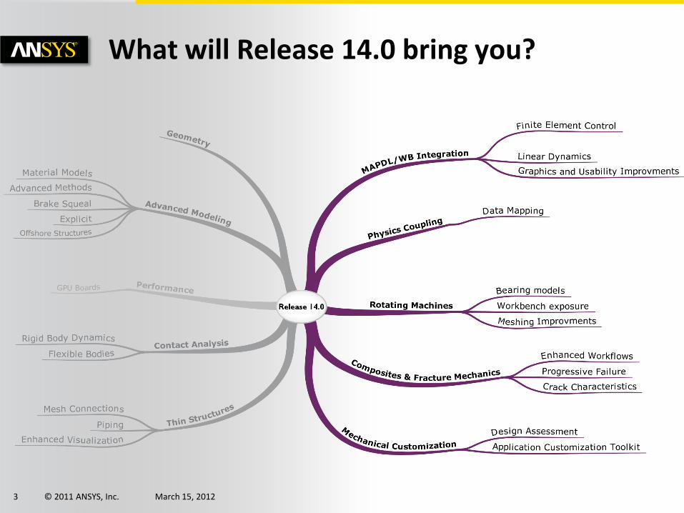
What will Release 14.0 bring you?
© 2011 ANSYS, Inc. March 15, 20124
MAPDL/WB Integration
Finite Element Information Access within ANSYS Mechanical
© 2011 ANSYS, Inc. March 15, 20125
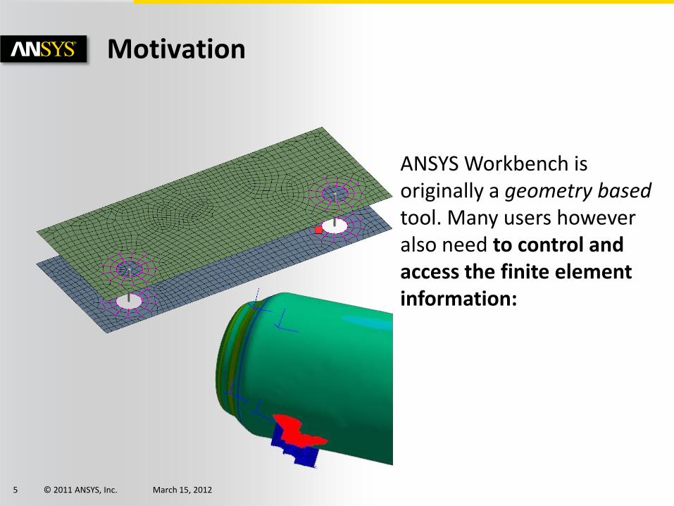
ANSYS Workbench is originally a geometry based tool. Many users however also need to control and access the finite element information:
Motivation
© 2011 ANSYS, Inc. March 15, 20126
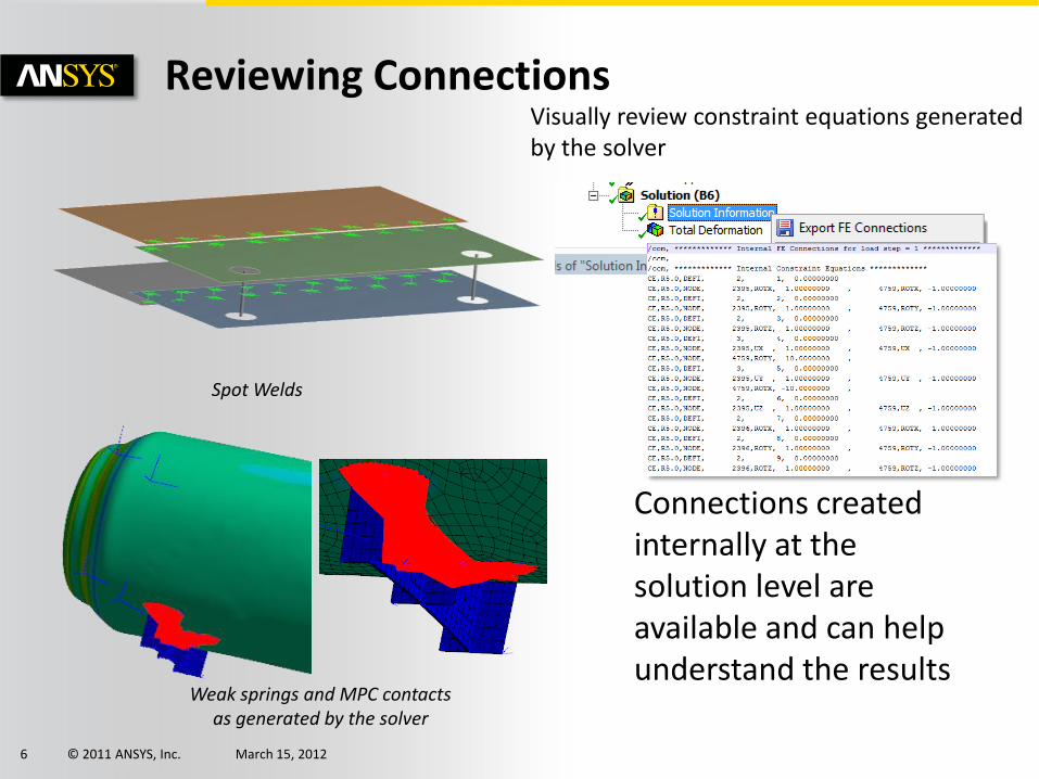
Spot Welds
Connections created internally at the solution level are available and can help understand the results
Reviewing Connections
Weak springs and MPC contacts as generated by the solver
Visually review constraint equations generated by the solver
© 2011 ANSYS, Inc. March 15, 20127
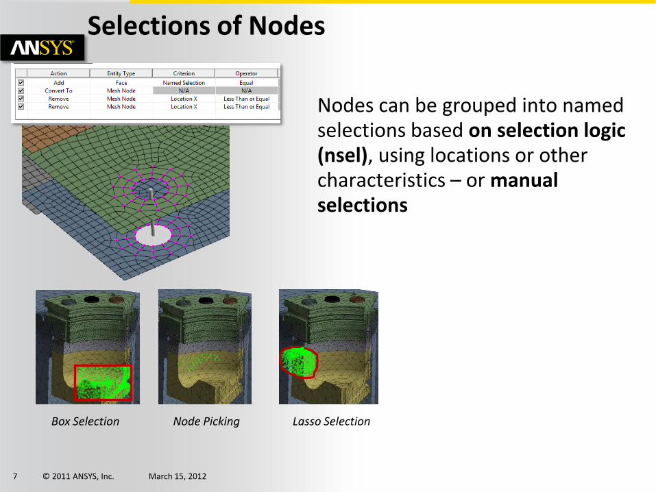
Nodes can be grouped into named selections based on selection logic (nsel), using locations or other characteristics – or manual selections
Selections of Nodes
Box Selection Node Picking Lasso Selection
© 2011 ANSYS, Inc. March 15, 20128
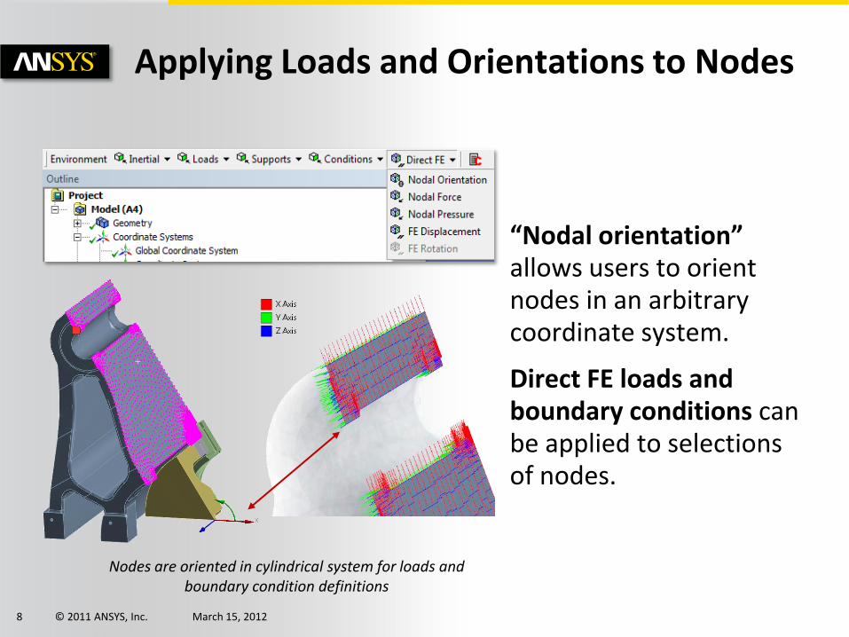
Applying Loads and Orientations to Nodes
“Nodal orientation” allows users to orient nodes in an arbitrary coordinate system.
Direct FE loads and boundary conditions can be applied to selections of nodes.
Nodes are oriented in cylindrical system for loads and boundary condition definitions
© 2011 ANSYS, Inc. March 15, 20129
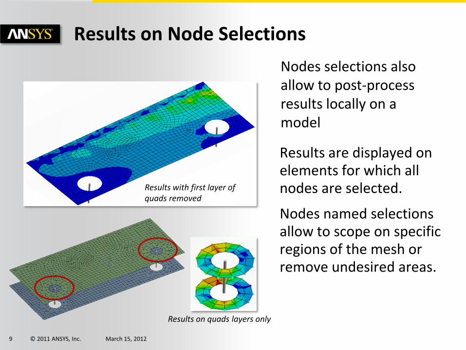
Results on Node Selections
Results are displayed on elements for which all nodes are selected.
Nodes named selections allow to scope on specific regions of the mesh or remove undesired areas.
Results with first layer of quads removed
Results on quads layers only
Nodes selections also allow to post-process results locally on a model
© 2011 ANSYS, Inc. March 15, 201210
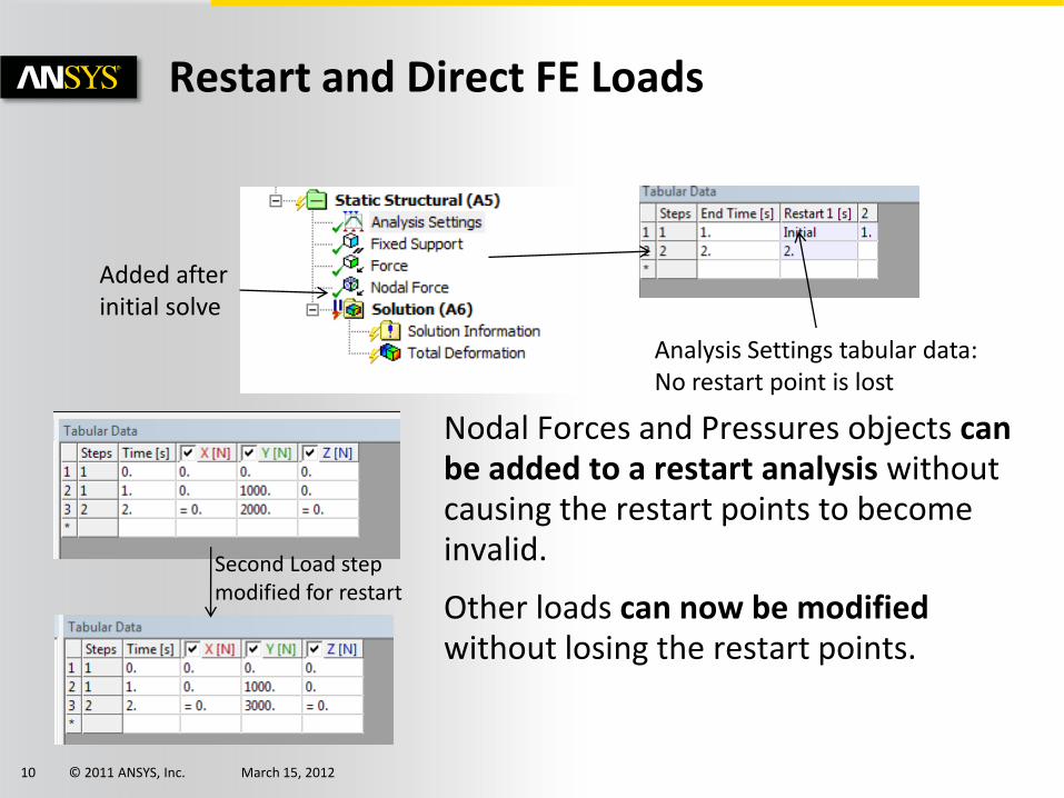
Restart and Direct FE Loads
Nodal Forces and Pressures objects can be added to a restart analysis without causing the restart points to become invalid.
Other loads can now be modified without losing the restart points.
Analysis Settings tabular data: No restart point is lost
Added after initial solve
Second Load step modified for restart
© 2011 ANSYS, Inc. March 15, 201211
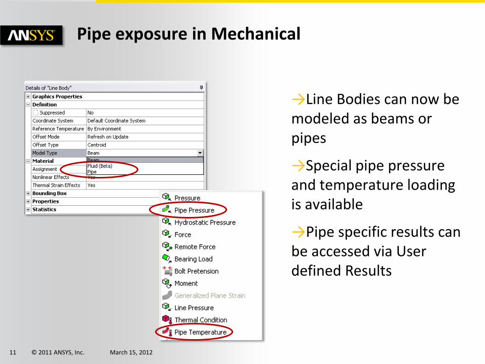
Pipe exposure in Mechanical
→Line Bodies can now be modeled as beams or pipes
→Special pipe pressure and temperature loading is available
→Pipe specific results can be accessed via User defined Results
© 2011 ANSYS, Inc. March 15, 201212
MAPDL/WB Integration
Linear Dynamics in ANSYS Mechanical
© 2011 ANSYS, Inc. March 15, 201213
MSUP Transient Analysis
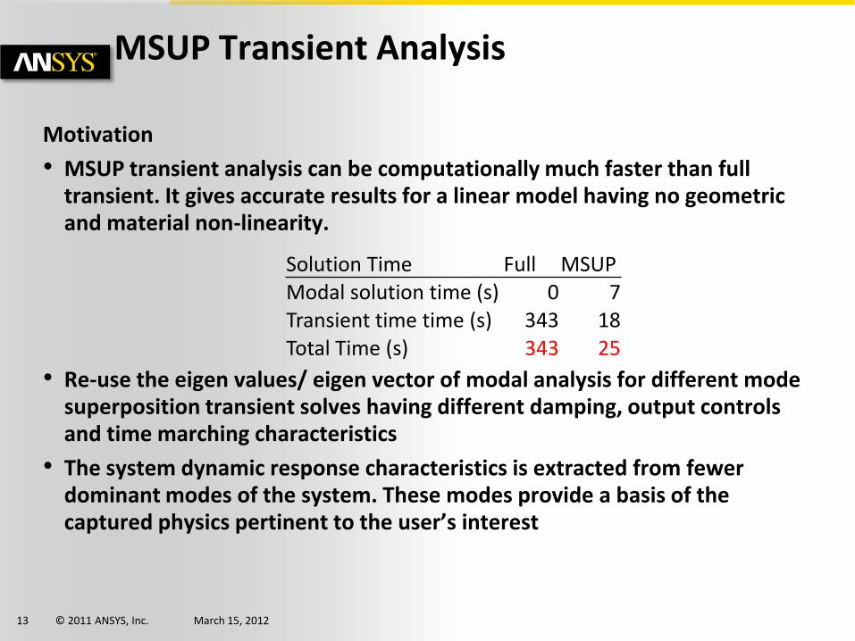
Motivation
• MSUP transient analysis can be computationally much faster than full transient. It gives accurate results for a linear model having no geometric and material non-linearity.
• Re-use the eigen values/ eigen vector of modal analysis for different mode superposition transient solves having different damping, output controls and time marching characteristics
• The system dynamic response characteristics is extracted from fewer dominant modes of the system. These modes provide a basis of the captured physics pertinent to the user’s interest
Solution Time Full MSUPModal solution time (s) 0 7Transient time time (s) 343 18Total Time (s) 343 25
© 2011 ANSYS, Inc. March 15, 201214
MSUP Transient Analysis(Contd)
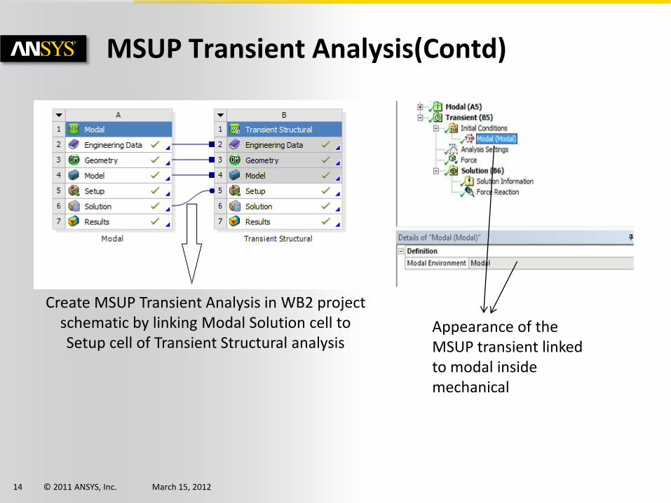
Create MSUP Transient Analysis in WB2 project schematic by linking Modal Solution cell to Setup cell of Transient Structural analysis
Appearance of the MSUP transient linkedto modal inside mechanical
© 2011 ANSYS, Inc. March 15, 201215
Workbench and Mechanical enhancements
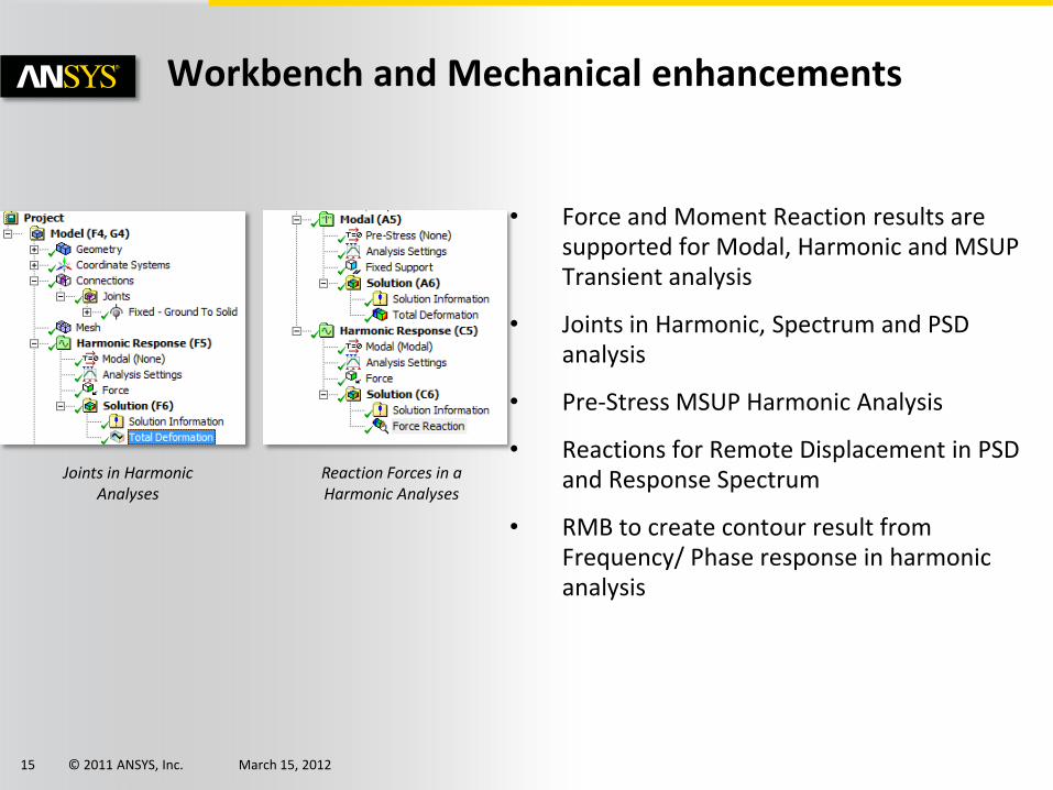
• Force and Moment Reaction results are supported for Modal, Harmonic and MSUP Transient analysis
• Joints in Harmonic, Spectrum and PSD analysis
• Pre-Stress MSUP Harmonic Analysis
• Reactions for Remote Displacement in PSD and Response Spectrum
• RMB to create contour result from Frequency/ Phase response in harmonic analysis
Joints in HarmonicAnalyses
Reaction Forces in a Harmonic Analyses
© 2011 ANSYS, Inc. March 15, 201216
Physics Coupling
Data Mapping
© 2011 ANSYS, Inc. March 15, 201217
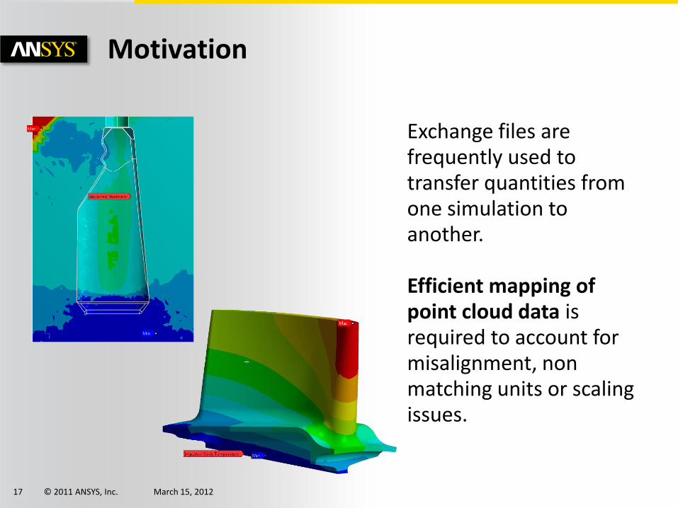
Motivation
Exchange files are frequently used to transfer quantities from one simulation to another.
Efficient mapping of point cloud data is required to account for misalignment, non matching units or scaling issues.
© 2011 ANSYS, Inc. March 15, 201218
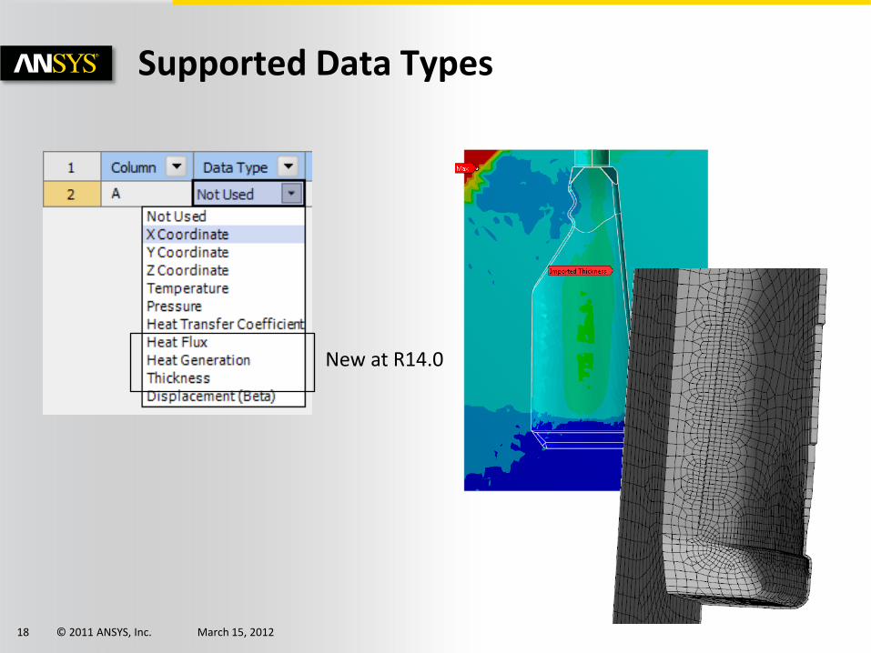
Supported Data Types
New at R14.0
© 2011 ANSYS, Inc. March 15, 201219
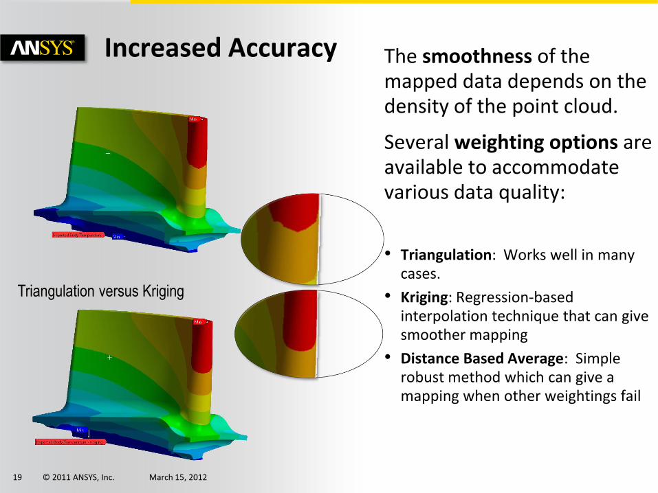
Increased Accuracy The smoothness of the mapped data depends on the density of the point cloud.
Several weighting options are available to accommodate various data quality:
• Triangulation: Works well in many cases.
• Kriging: Regression-based interpolation technique that can give smoother mapping
• Distance Based Average: Simple robust method which can give a mapping when other weightings fail
Triangulation versus Kriging
© 2011 ANSYS, Inc. March 15, 201220
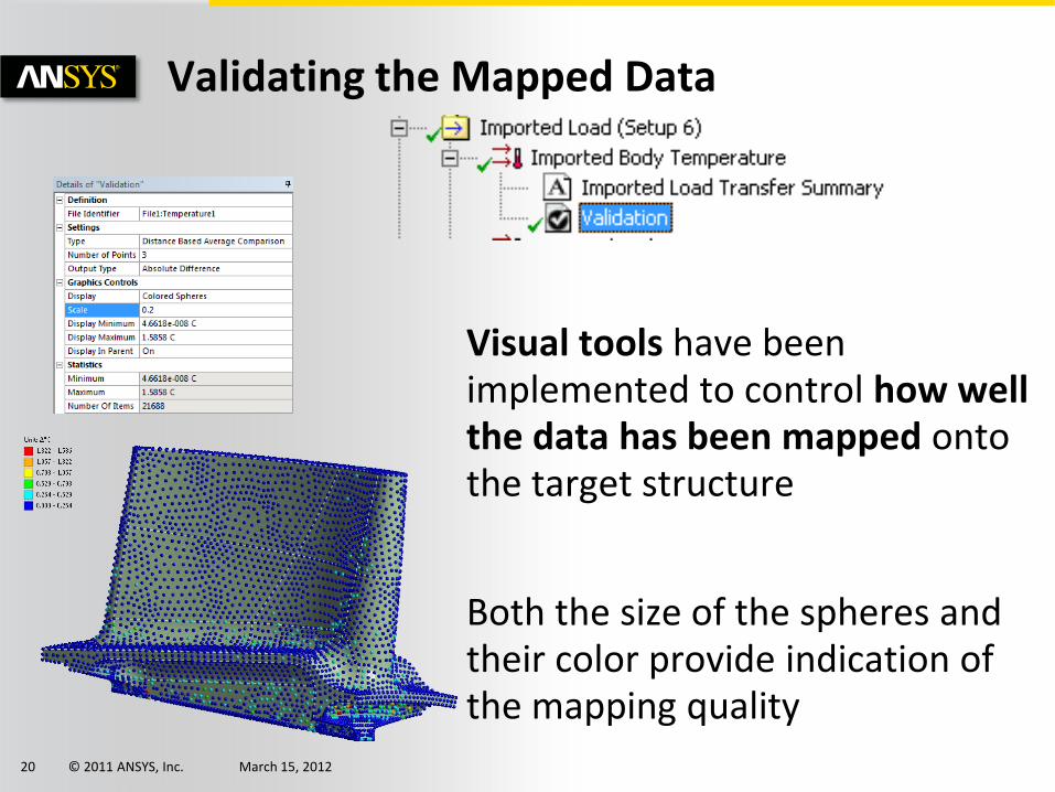
Validating the Mapped Data
Visual tools have been implemented to control how well the data has been mapped onto the target structure
Both the size of the spheres and their color provide indication of the mapping quality

© 2011 ANSYS, Inc. March 15, 201221
Importing Multiple Files
Multiple files can be imported for transient analyses or to handle different data to be mapped on multiple bodies
© 2011 ANSYS, Inc. March 15, 201222
Rotating Machines
Studying Rotordynamics in ANSYS Mechanical
© 2011 ANSYS, Inc. March 15, 201223
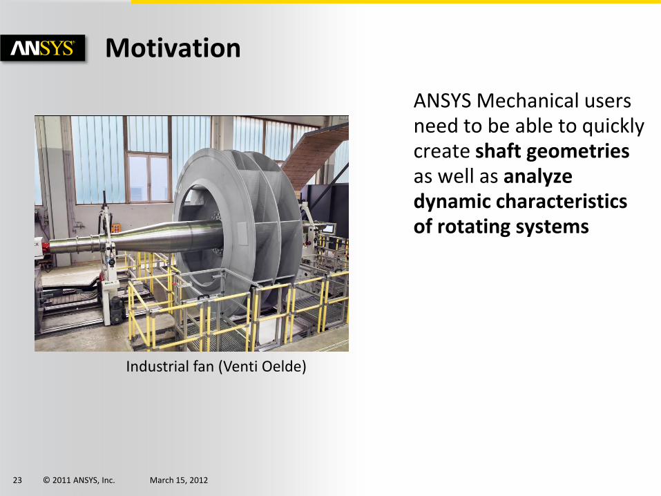
Motivation
ANSYS Mechanical users need to be able to quickly create shaft geometriesas well as analyze dynamic characteristics of rotating systems
Industrial fan (Venti Oelde)
© 2011 ANSYS, Inc. March 15, 201224
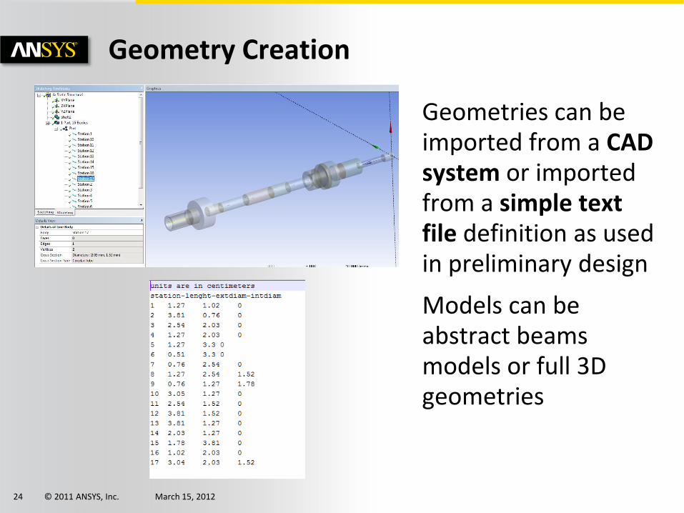
Geometry Creation
Geometries can be imported from a CAD system or imported from a simple text file definition as used in preliminary design
Models can be abstract beams models or full 3D geometries
© 2011 ANSYS, Inc. March 15, 201225
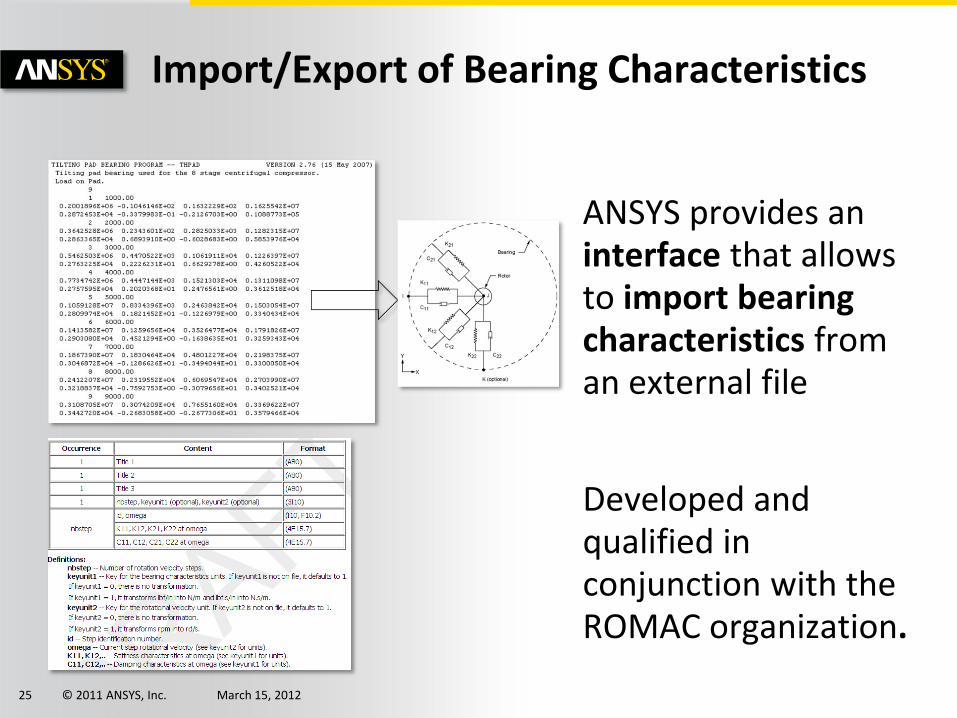
Import/Export of Bearing Characteristics
ANSYS provides an interface that allows to import bearing characteristics from an external file
Developed and qualified in conjunction with the ROMAC organization.
© 2011 ANSYS, Inc. March 15, 201226
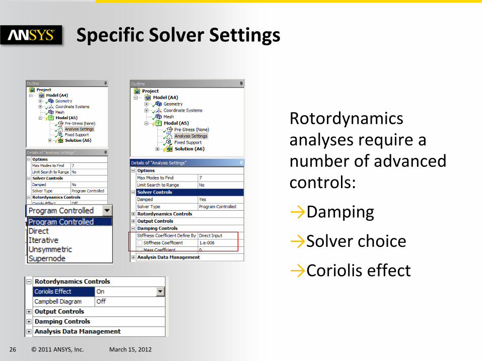
Specific Solver Settings
Rotordynamicsanalyses require a number of advanced controls:
→Damping
→Solver choice
→Coriolis effect
© 2011 ANSYS, Inc. March 15, 201227
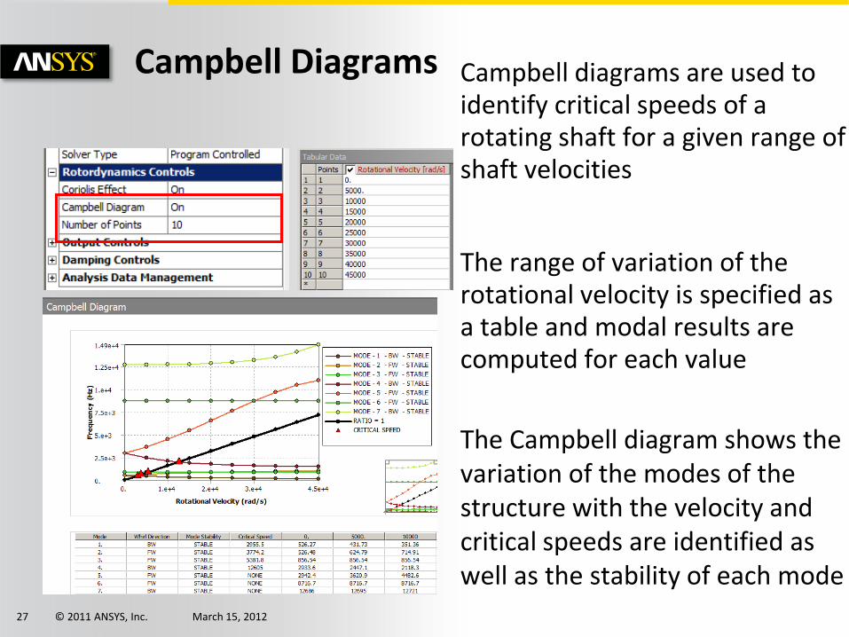
Campbell Diagrams Campbell diagrams are used to identify critical speeds of a rotating shaft for a given range of shaft velocities
The range of variation of the rotational velocity is specified as a table and modal results are computed for each value
The Campbell diagram shows the variation of the modes of the structure with the velocity and critical speeds are identified as well as the stability of each mode
© 2011 ANSYS, Inc. March 15, 201228
Composites
Enhanced Analysis Workflow and Advanced Failure Models for Composites
© 2011 ANSYS, Inc. March 15, 201229
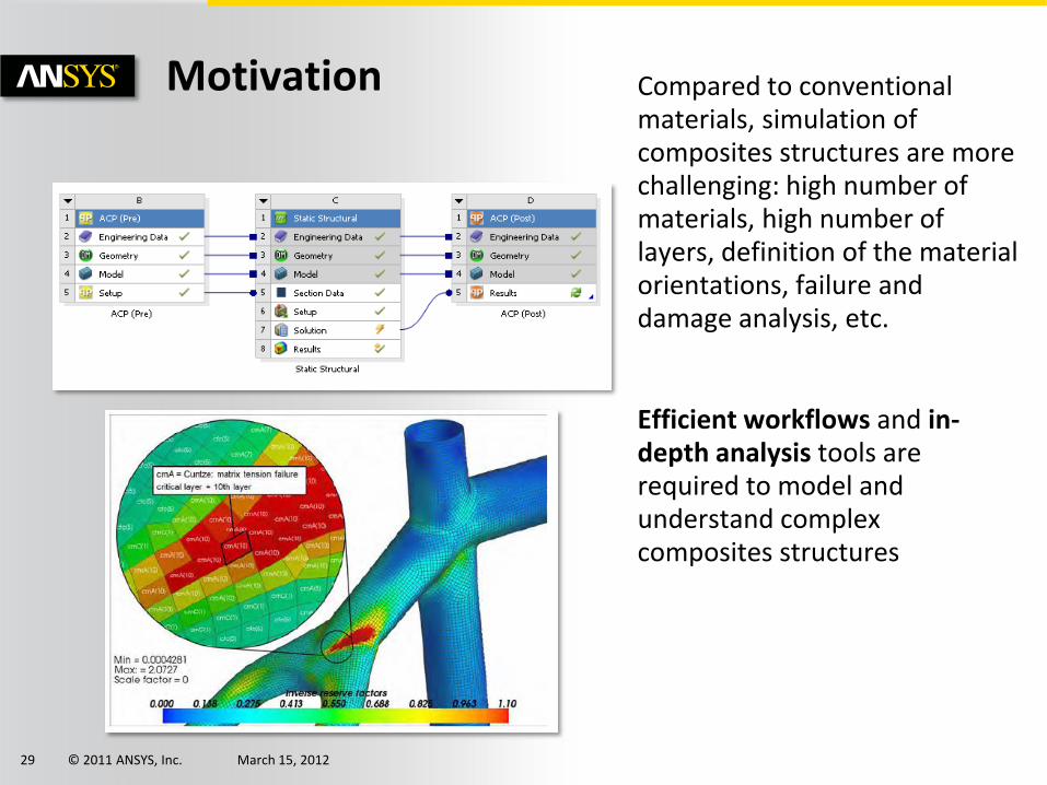
Motivation Compared to conventional materials, simulation of composites structures are more challenging: high number of materials, high number of layers, definition of the material orientations, failure and damage analysis, etc.
Efficient workflows and in-depth analysis tools are required to model and understand complex composites structures
© 2011 ANSYS, Inc. March 15, 201230
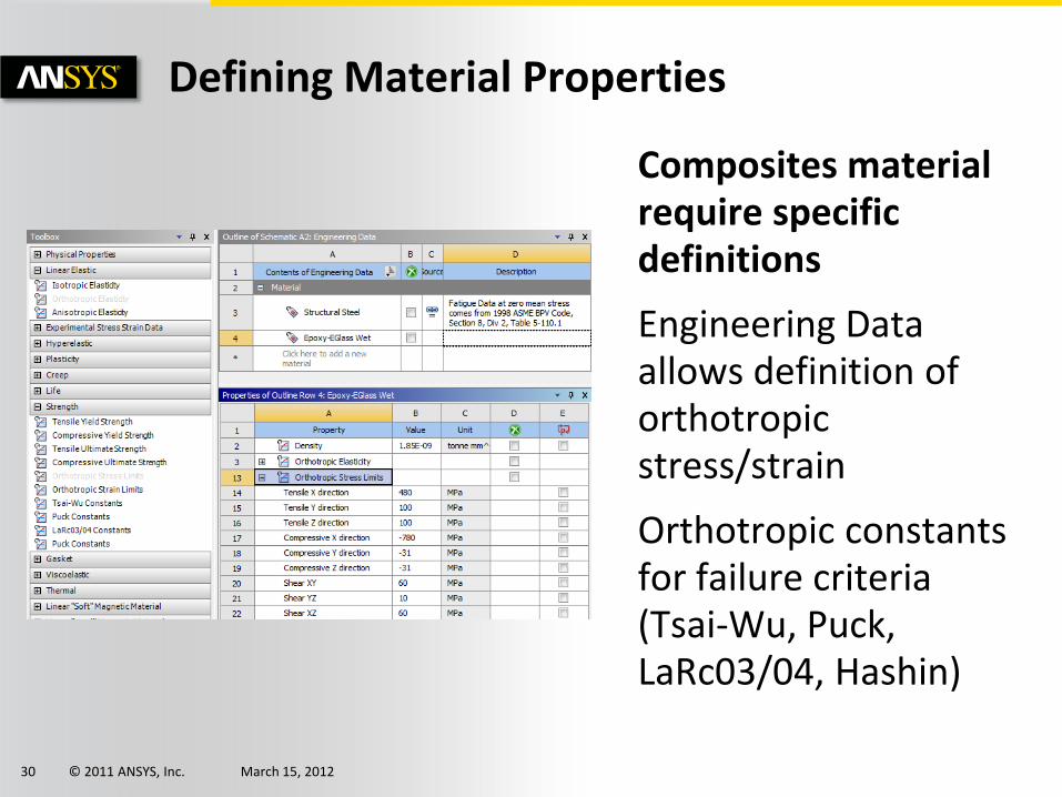
Defining Material Properties
Composites material require specific definitions
Engineering Data allows definition of orthotropic stress/strain
Orthotropic constants for failure criteria (Tsai-Wu, Puck, LaRc03/04, Hashin)
© 2011 ANSYS, Inc. March 15, 201231
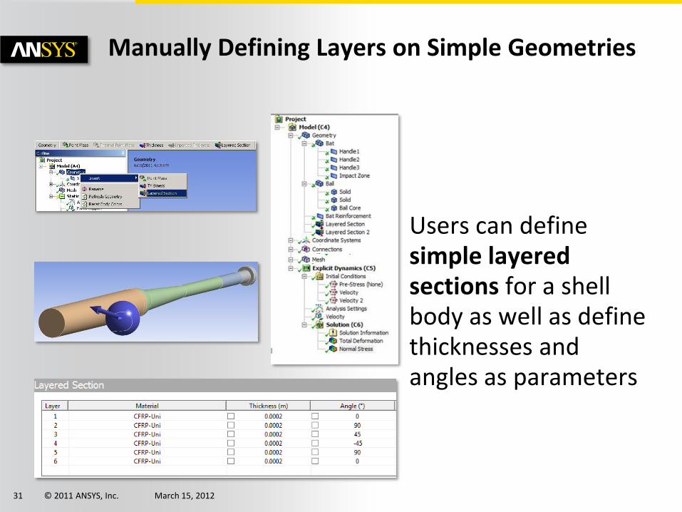
Manually Defining Layers on Simple Geometries
Users can define simple layered sections for a shell body as well as define thicknesses and angles as parameters
© 2011 ANSYS, Inc. March 15, 201232
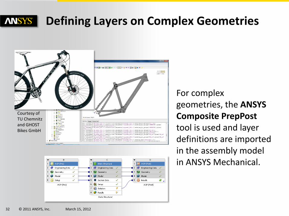
Defining Layers on Complex Geometries
For complex geometries, the ANSYS Composite PrepPosttool is used and layer definitions are imported in the assembly model in ANSYS Mechanical.
Courtesy of TU Chemnitz and GHOST Bikes GmbH
© 2011 ANSYS, Inc. March 15, 201233
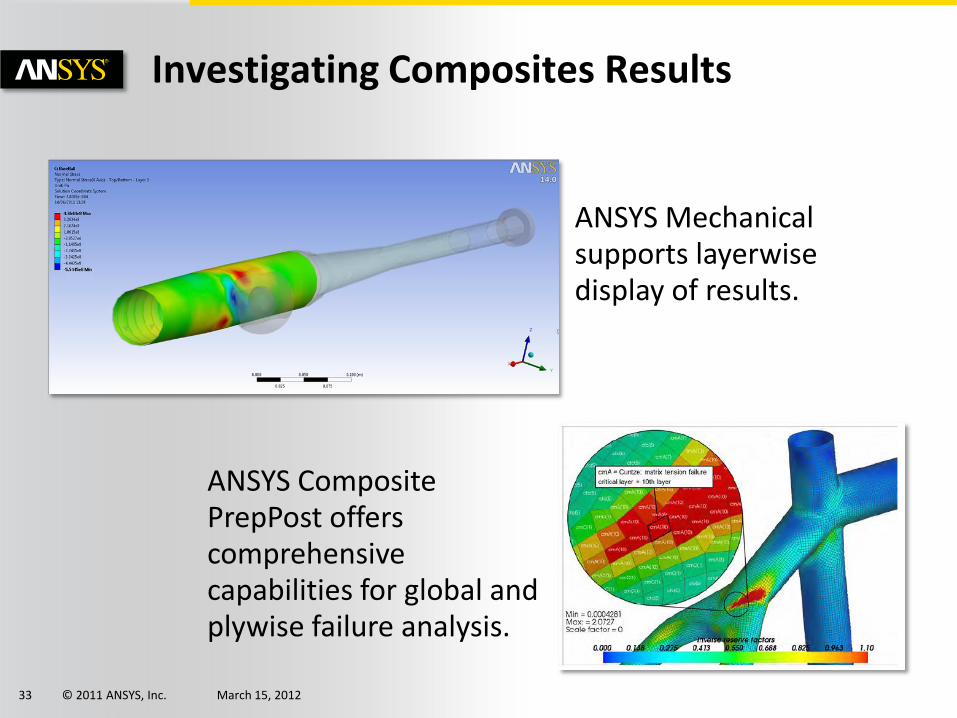
Investigating Composites Results
ANSYS Mechanicalsupports layerwisedisplay of results.
ANSYS Composite PrepPost offers comprehensive capabilities for global and plywise failure analysis.
© 2011 ANSYS, Inc. March 15, 201234
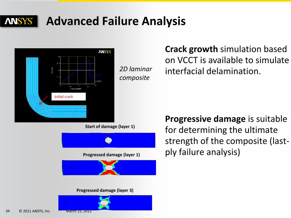
Advanced Failure Analysis
Crack growth simulation based on VCCT is available to simulate interfacial delamination.
Progressive damage is suitable for determining the ultimate strength of the composite (last-ply failure analysis)
2D laminar composite
Initial crack
Start of damage (layer 1)
Progressed damage (layer 1)
Progressed damage (layer 3)
© 2011 ANSYS, Inc. March 15, 201235
Customization
ANSYS Design Assessment
© 2011 ANSYS, Inc. March 15, 201236
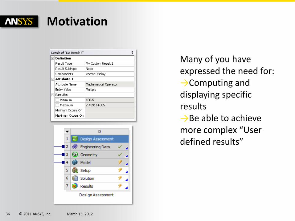
Motivation
Many of you have expressed the need for:→Computing and displaying specific results→Be able to achieve more complex “User defined results”
© 2011 ANSYS, Inc. March 15, 201237
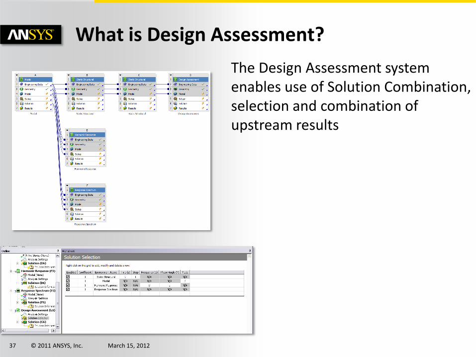
What is Design Assessment?
The Design Assessment system enables use of Solution Combination, selection and combination of upstream results
© 2011 ANSYS, Inc. March 15, 201239
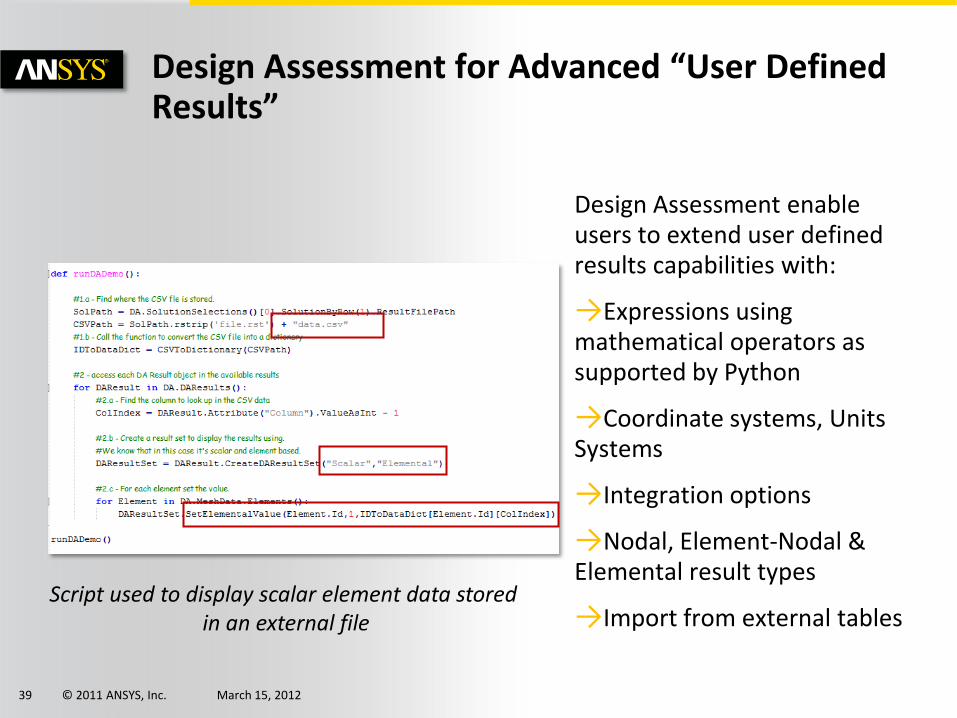
Design Assessment for Advanced “User Defined Results”
Design Assessment enable users to extend user defined results capabilities with:
→Expressions using mathematical operators as supported by Python
→Coordinate systems, Units Systems
→Integration options
→Nodal, Element-Nodal & Elemental result types
→Import from external tablesScript used to display scalar element data stored
in an external file
© 2011 ANSYS, Inc. March 15, 201240
Customization
Application Customization Toolkit
© 2011 ANSYS, Inc. March 15, 201241
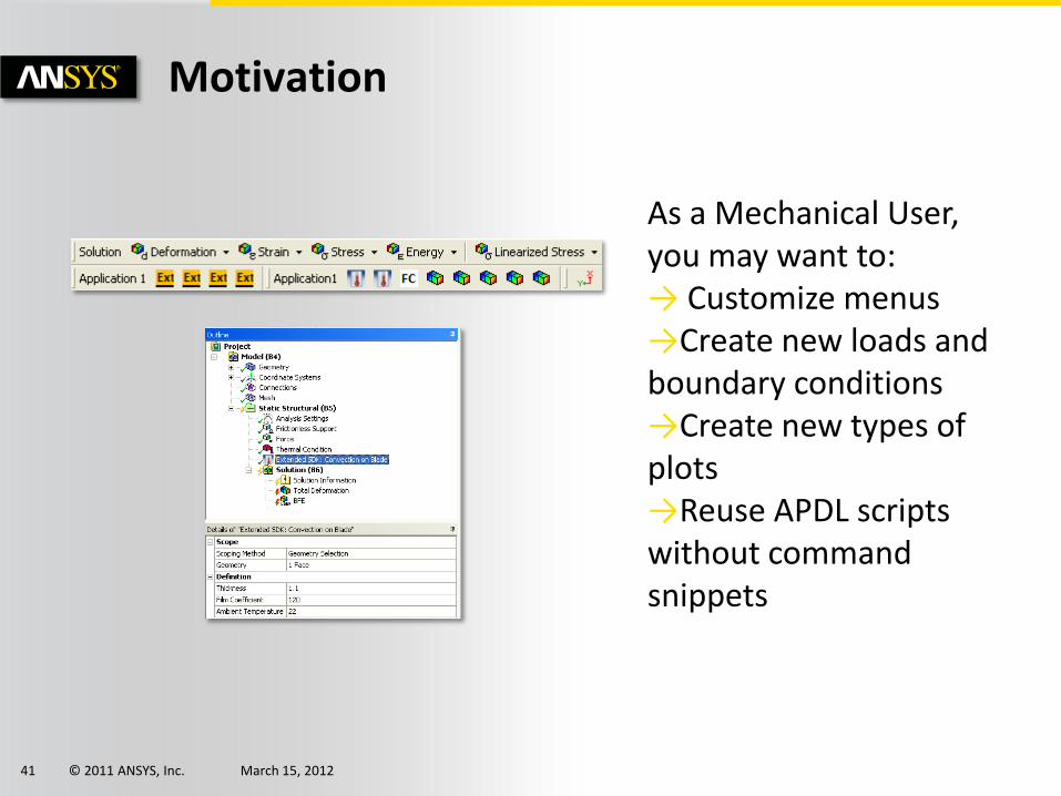
Motivation
As a Mechanical User, you may want to:→ Customize menus→Create new loads and boundary conditions→Create new types of plots→Reuse APDL scripts without command snippets
© 2011 ANSYS, Inc. March 15, 201242
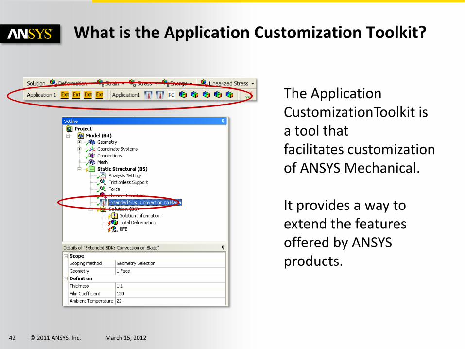
What is the Application Customization Toolkit?
The Application CustomizationToolkit is a tool that facilitates customization of ANSYS Mechanical.
It provides a way to extend the features offered by ANSYS products.
© 2011 ANSYS, Inc. March 15, 201243
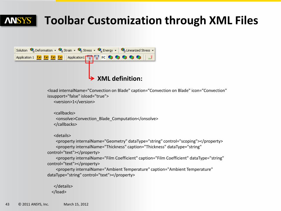
Toolbar Customization through XML Files
<load internalName="Convection on Blade" caption="Convection on Blade" icon="Convection" issupport="false" isload="true">
<version>1</version>
<callbacks><onsolve>Convection_Blade_Computation</onsolve>
</callbacks>
<details><property internalName="Geometry" dataType="string" control="scoping"></property><property internalName="Thickness" caption="Thickness" dataType="string"
control="text"></property><property internalName="Film Coefficient" caption="Film Coefficient" dataType="string"
control="text"></property><property internalName="Ambient Temperature" caption="Ambient Temperature"
dataType="string" control="text"></property>
</details></load>
XML definition:
© 2011 ANSYS, Inc. March 15, 201244
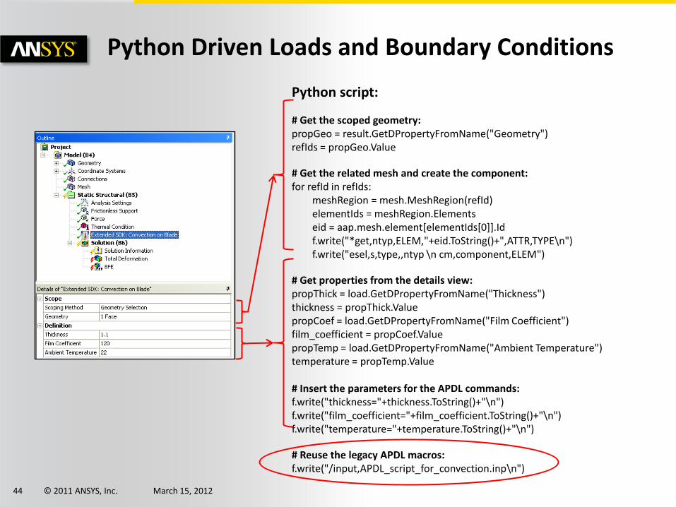
Python Driven Loads and Boundary Conditions
Python script:
# Get the scoped geometry:propGeo = result.GetDPropertyFromName("Geometry")refIds = propGeo.Value
# Get the related mesh and create the component:for refId in refIds:
meshRegion = mesh.MeshRegion(refId)elementIds = meshRegion.Elementseid = aap.mesh.element[elementIds[0]].Idf.write("*get,ntyp,ELEM,"+eid.ToString()+",ATTR,TYPE\n")f.write("esel,s,type,,ntyp \n cm,component,ELEM")
# Get properties from the details view:propThick = load.GetDPropertyFromName("Thickness")thickness = propThick.ValuepropCoef = load.GetDPropertyFromName("Film Coefficient")film_coefficient = propCoef.ValuepropTemp = load.GetDPropertyFromName("Ambient Temperature")temperature = propTemp.Value
# Insert the parameters for the APDL commands:f.write("thickness="+thickness.ToString()+"\n")f.write("film_coefficient="+film_coefficient.ToString()+"\n")f.write("temperature="+temperature.ToString()+"\n")
# Reuse the legacy APDL macros:f.write("/input,APDL_script_for_convection.inp\n")
© 2011 ANSYS, Inc. March 15, 201245
• Encapsulate APDL macros: Allows re-use of legacy APDL-scripts and encourages migration from MAPDL to Mechanical via “encapsulated macros”
• MAPDL exposure: Fills in the gap between the MAPDL solver capabilities and their exposition in ANSYS Mechanical
• Adding new pre-processing features (custom loads and boundary conditions)
• Adding new post-processing features (results)
• 3rd party/in-house solver integration (Mechanical GUI)
ACT scope at R14.0
© 2011 ANSYS, Inc. March 15, 201246
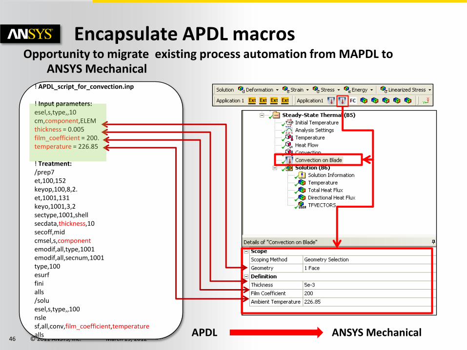
Opportunity to migrate existing process automation from MAPDL to ANSYS Mechanical
Encapsulate APDL macros
APDL
! APDL_script_for_convection.inp
! Input parameters:esel,s,type,,10cm,component,ELEMthickness = 0.005film_coefficient = 200.temperature = 226.85
! Treatment:/prep7et,100,152keyop,100,8,2.et,1001,131keyo,1001,3,2sectype,1001,shellsecdata,thickness,10secoff,midcmsel,s,componentemodif,all,type,1001emodif,all,secnum,1001type,100esurffinialls/soluesel,s,type,,100nslesf,all,conv,film_coefficient,temperaturealls APDL ANSYS Mechanical
© 2011 ANSYS, Inc. March 15, 201247
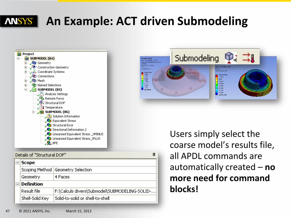
An Example: ACT driven Submodeling
Users simply select the coarse model’s results file, all APDL commands are automatically created – no more need for command blocks!
© 2011 ANSYS, Inc. March 15, 201248
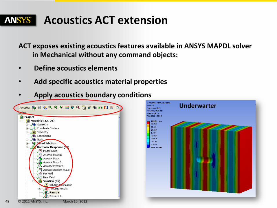
ACT exposes existing acoustics features available in ANSYS MAPDL solver in Mechanical without any command objects:
• Define acoustics elements
• Add specific acoustics material properties
• Apply acoustics boundary conditions
Acoustics ACT extension
Underwarter
© 2011 ANSYS, Inc. March 15, 201249
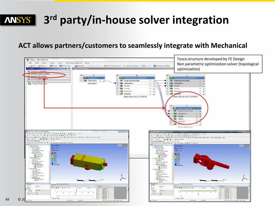
ACT allows partners/customers to seamlessly integrate with Mechanical
3rd party/in-house solver integration
Tosca structure developed by FE DesignNon parametric optimization solver (topological optimization)

© 2011 ANSYS, Inc. March 15, 201250
R 14 Update
© 2011 ANSYS, Inc. March 15, 201251
What will Release 14.0 bring you?
© 2011 ANSYS, Inc. March 15, 201252
Advanced Modeling
Material Models
© 2011 ANSYS, Inc. March 15, 201253
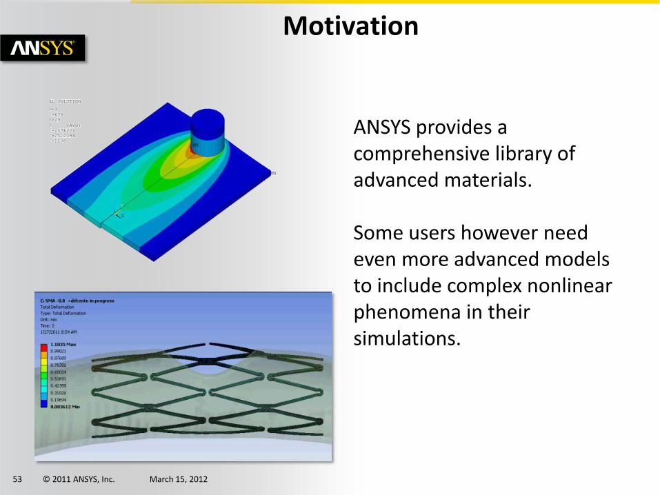
Motivation
ANSYS provides a comprehensive library of advanced materials.
Some users however need even more advanced models to include complex nonlinear phenomena in their simulations.
© 2011 ANSYS, Inc. March 15, 201254
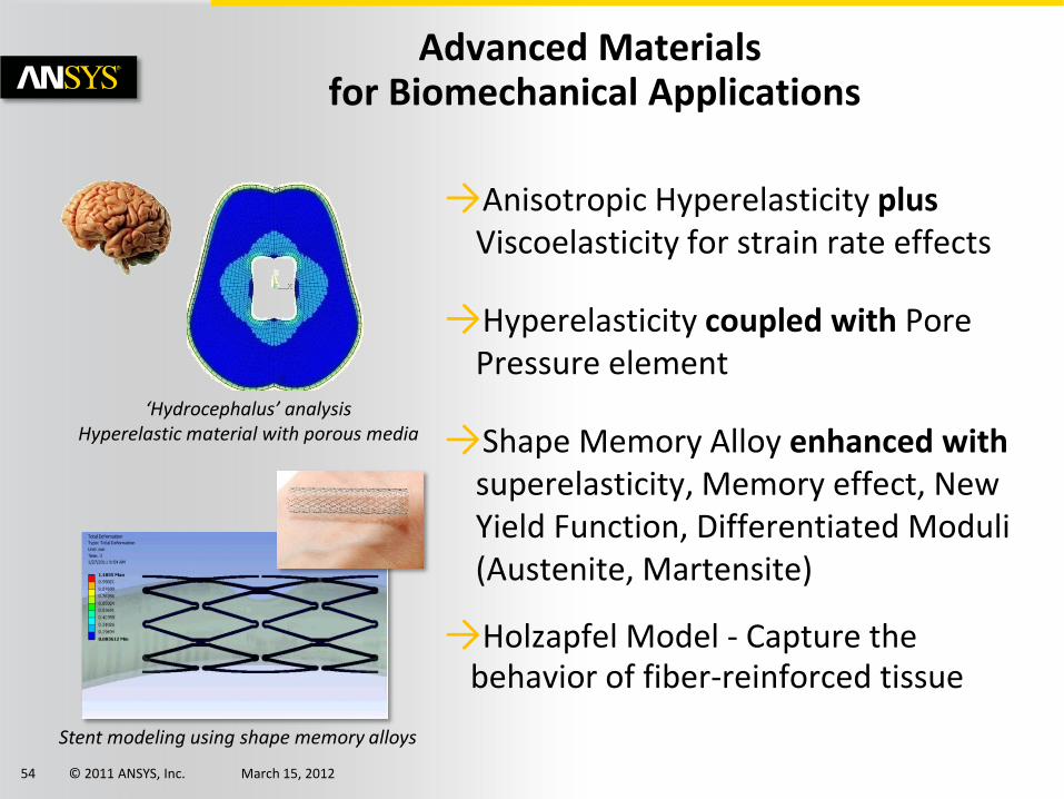
→Anisotropic Hyperelasticity plusViscoelasticity for strain rate effects
→Hyperelasticity coupled with Pore Pressure element
→Shape Memory Alloy enhanced with superelasticity, Memory effect, New Yield Function, Differentiated Moduli (Austenite, Martensite)
→Holzapfel Model - Capture the behavior of fiber-reinforced tissue
Advanced Materialsfor Biomechanical Applications
‘Hydrocephalus’ analysis Hyperelastic material with porous media
Stent modeling using shape memory alloys
© 2011 ANSYS, Inc. March 15, 201255
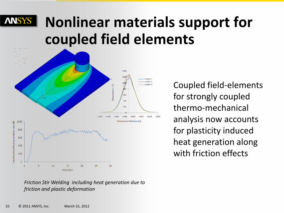
Nonlinear materials support for coupled field elements
Coupled field-elements for strongly coupled thermo-mechanical analysis now accounts for plasticity induced heat generation along with friction effects
Friction Stir Welding including heat generation due to friction and plastic deformation
© 2011 ANSYS, Inc. March 15, 201256
Advanced Modeling
Advanced Methods
© 2011 ANSYS, Inc. March 15, 201257
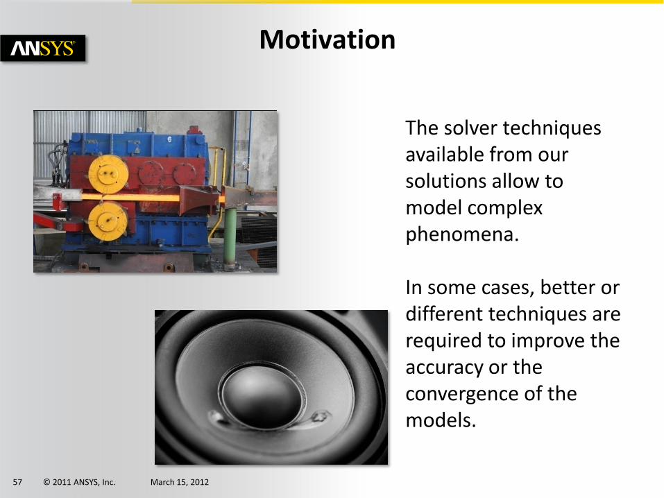
Motivation
The solver techniques available from our solutions allow to model complex phenomena.
In some cases, better or different techniques are required to improve the accuracy or the convergence of the models.
© 2011 ANSYS, Inc. March 15, 201258
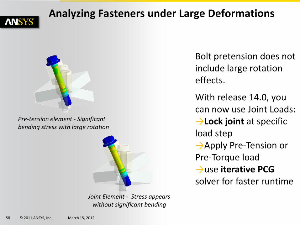
Analyzing Fasteners under Large Deformations
Bolt pretension does not include large rotation effects.
With release 14.0, you can now use Joint Loads:→Lock joint at specific load step→Apply Pre-Tension or Pre-Torque load→use iterative PCG solver for faster runtime
Joint Element - Stress appears without significant bending
Pre-tension element - Significant bending stress with large rotation
© 2011 ANSYS, Inc. March 15, 201259
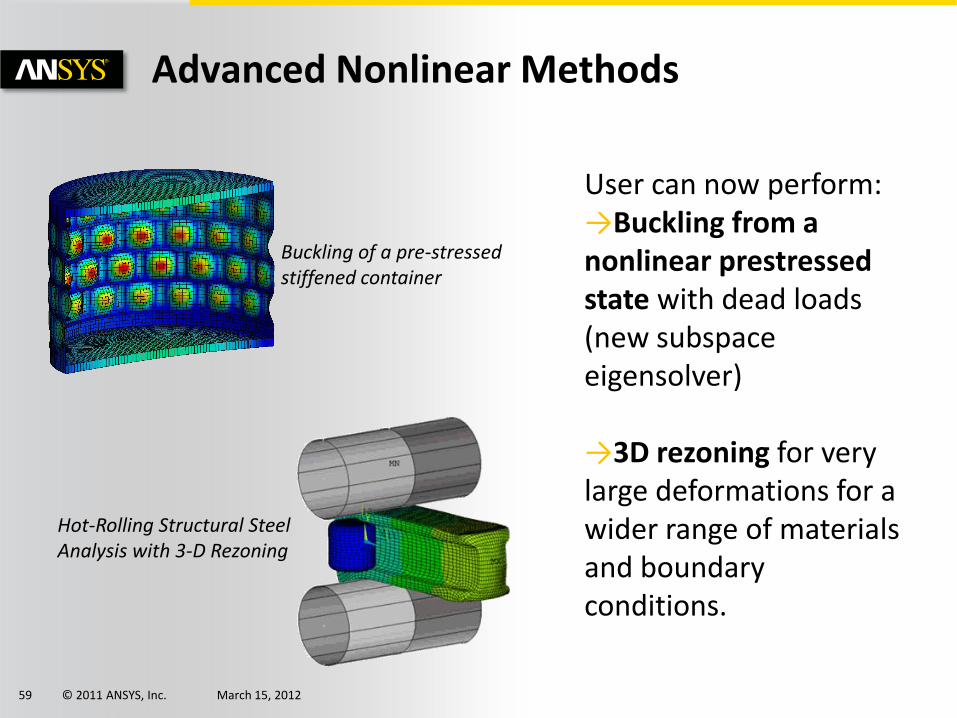
Advanced Nonlinear Methods
User can now perform:→Buckling from a nonlinear prestressedstate with dead loads (new subspace eigensolver)
→3D rezoning for very large deformations for a wider range of materials and boundary conditions.
Hot-Rolling Structural Steel Analysis with 3-D Rezoning
Buckling of a pre-stressed stiffened container
© 2011 ANSYS, Inc. March 15, 201260
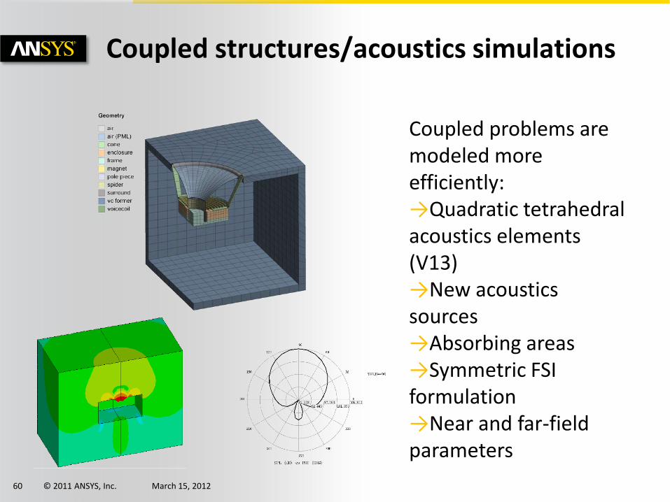
Coupled structures/acoustics simulations
Coupled problems are modeled more efficiently:→Quadratic tetrahedral acoustics elements (V13)→New acoustics sources→Absorbing areas→Symmetric FSI formulation→Near and far-field parameters
© 2011 ANSYS, Inc. March 15, 201261
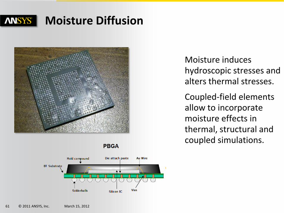
Moisture Diffusion
Moisture induces hydroscopic stresses and alters thermal stresses.
Coupled-field elements allow to incorporate moisture effects in thermal, structural and coupled simulations.
© 2011 ANSYS, Inc. March 15, 201262
Advanced Modeling
Explicit Analysis
© 2011 ANSYS, Inc. March 15, 201263
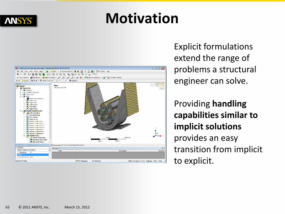
Motivation
Explicit formulations extend the range of problems a structural engineer can solve.
Providing handling capabilities similar to implicit solutions provides an easy transition from implicit to explicit.

© 2011 ANSYS, Inc. March 15, 201264
Common User Interface
Implicit and explicit solutions share the same user interface for a shortened learning curve and allow straightforward data exchange between disciplines
Crimping
© 2011 ANSYS, Inc. March 15, 201265
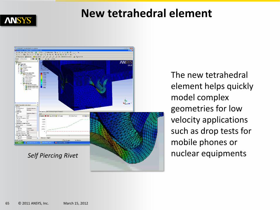
New tetrahedral element
The new tetrahedral element helps quickly model complex geometries for low velocity applications such as drop tests for mobile phones or nuclear equipmentsSelf Piercing Rivet
© 2011 ANSYS, Inc. March 15, 201266
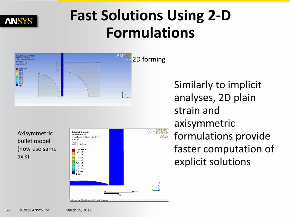
Similarly to implicit analyses, 2D plain strain and axisymmetricformulations provide faster computation of explicit solutions
Fast Solutions Using 2-D Formulations
2D forming
Axisymmetricbullet model (now use same axis)

© 2011 ANSYS, Inc. March 15, 201267
Performance
Further benefits from GPU boards
© 2011 ANSYS, Inc. March 15, 201268
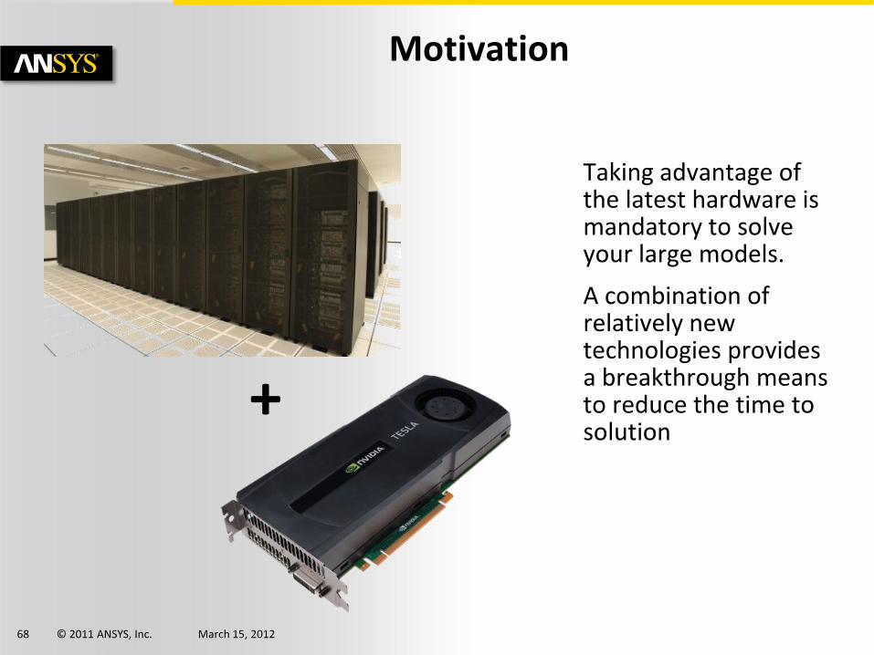
Taking advantage of the latest hardware is mandatory to solve your large models.
A combination of relatively new technologies provides a breakthrough means to reduce the time to solution
Motivation
+
© 2011 ANSYS, Inc. March 15, 201269
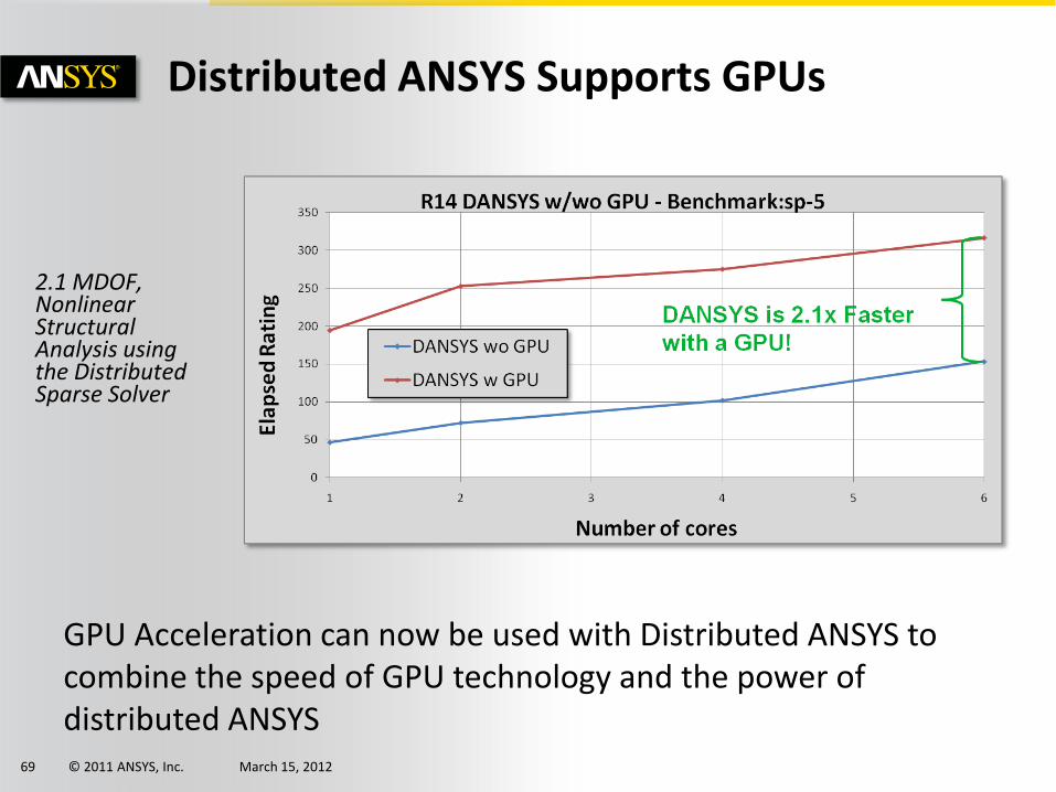
Distributed ANSYS Supports GPUs
2.1 MDOF, Nonlinear Structural Analysis using the Distributed Sparse Solver
GPU Acceleration can now be used with Distributed ANSYS to combine the speed of GPU technology and the power of distributed ANSYS
© 2011 ANSYS, Inc. March 15, 201270
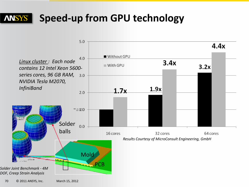
Speed-up from GPU technology
Solder Joint Benchmark - 4M DOF, Creep Strain Analysis
Results Courtesy of MicroConsult Engineering, GmbH
Linux cluster : Each node contains 12 Intel Xeon 5600-series cores, 96 GB RAM, NVIDIA Tesla M2070, InfiniBand
Mold
PCB
Solder balls
© 2011 ANSYS, Inc. March 15, 201271
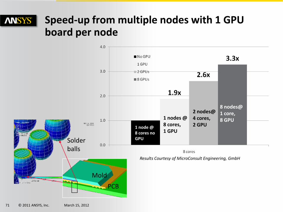
Speed-up from multiple nodes with 1 GPU board per node
Mold
PCB
Solder balls
Results Courtesy of MicroConsult Engineering, GmbH
1 node @ 8 cores no GPU
1 nodes @ 8 cores, 1 GPU
8 nodes@ 1 core, 8 GPU
2 nodes@ 4 cores, 2 GPU
© 2011 ANSYS, Inc. March 15, 201272
Mesh Connections
© 2011 ANSYS, Inc. March 15, 201273
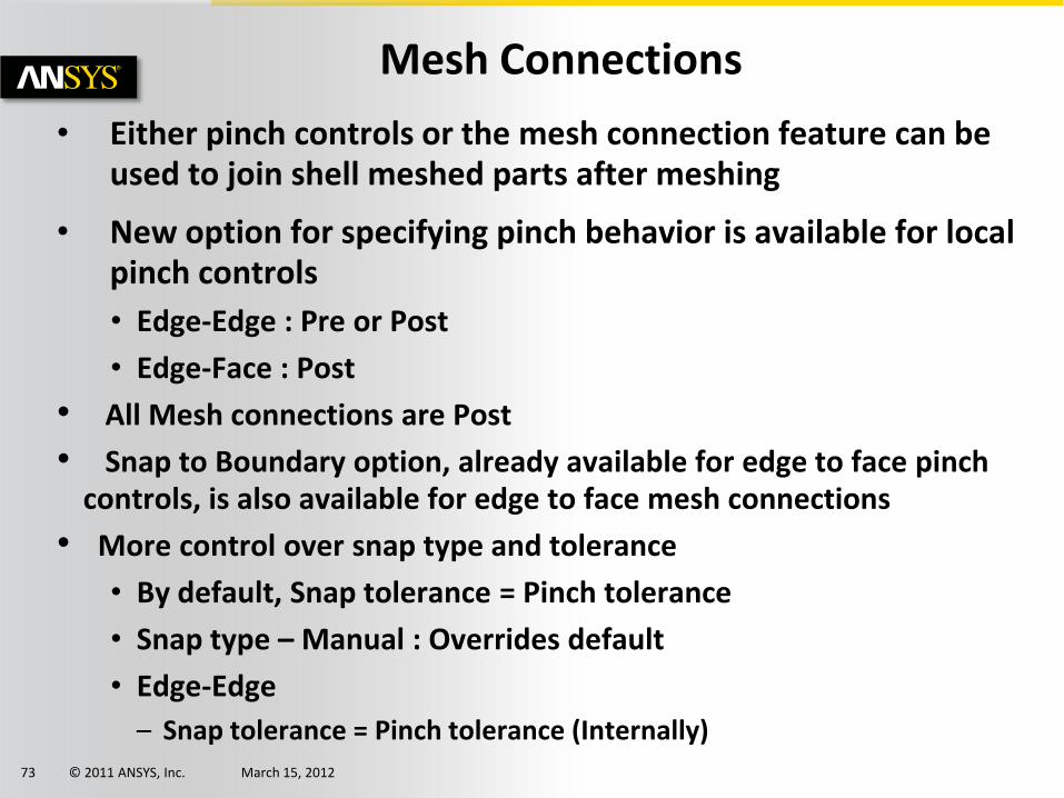
Mesh Connections
• Either pinch controls or the mesh connection feature can be used to join shell meshed parts after meshing
• New option for specifying pinch behavior is available for local pinch controls
• Edge-Edge : Pre or Post
• Edge-Face : Post
• All Mesh connections are Post
• Snap to Boundary option, already available for edge to face pinch controls, is also available for edge to face mesh connections
• More control over snap type and tolerance
• By default, Snap tolerance = Pinch tolerance
• Snap type – Manual : Overrides default
• Edge-Edge
– Snap tolerance = Pinch tolerance (Internally)
© 2011 ANSYS, Inc. March 15, 201274
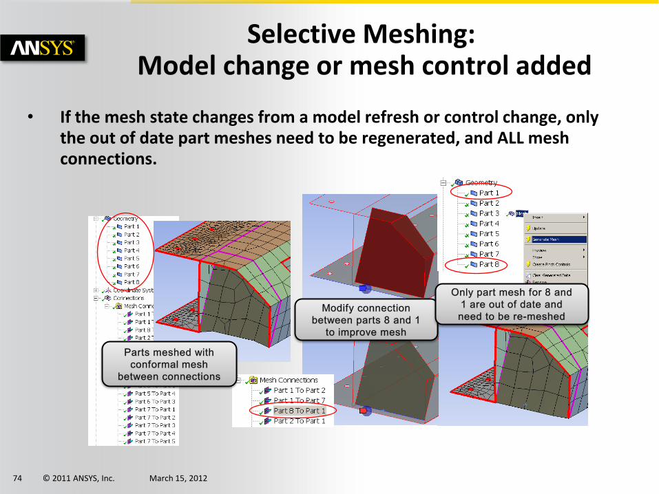
Selective Meshing:Model change or mesh control added
• If the mesh state changes from a model refresh or control change, only the out of date part meshes need to be regenerated, and ALL mesh connections.
© 2011 ANSYS, Inc. March 15, 201275
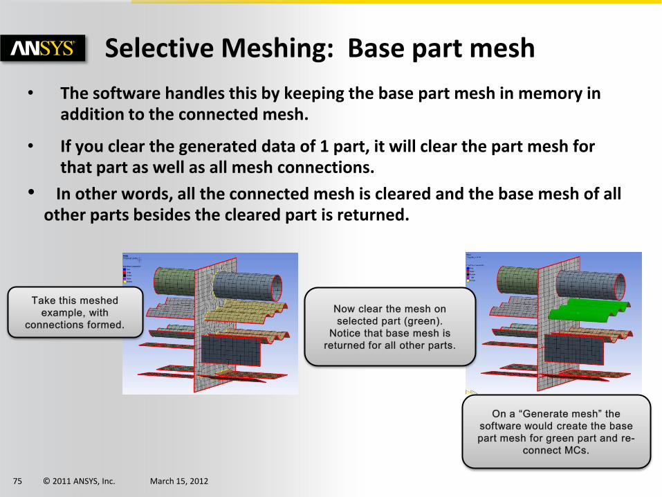
Selective Meshing: Base part mesh
• The software handles this by keeping the base part mesh in memory in addition to the connected mesh.
• If you clear the generated data of 1 part, it will clear the part mesh for that part as well as all mesh connections.
• In other words, all the connected mesh is cleared and the base mesh of all other parts besides the cleared part is returned.
© 2011 ANSYS, Inc. March 15, 201276
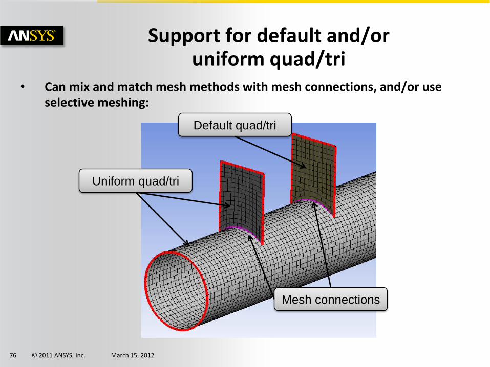
Support for default and/or uniform quad/tri
• Can mix and match mesh methods with mesh connections, and/or use selective meshing:
Uniform quad/tri
Default quad/tri
Mesh connections
© 2011 ANSYS, Inc. March 15, 201277
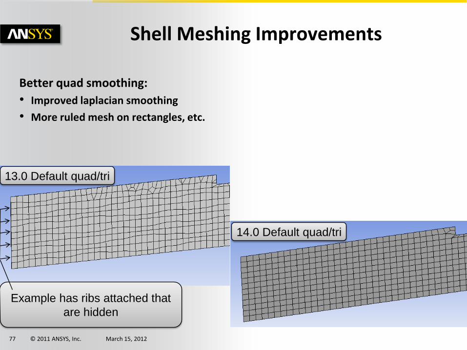
Shell Meshing Improvements
Better quad smoothing:
• Improved laplacian smoothing
• More ruled mesh on rectangles, etc.
13.0 Default quad/tri
14.0 Default quad/tri
Example has ribs attached that
are hidden
© 2011 ANSYS, Inc. March 15, 201278
Mesh Connections :Visualization
© 2011 ANSYS, Inc. March 15, 201279
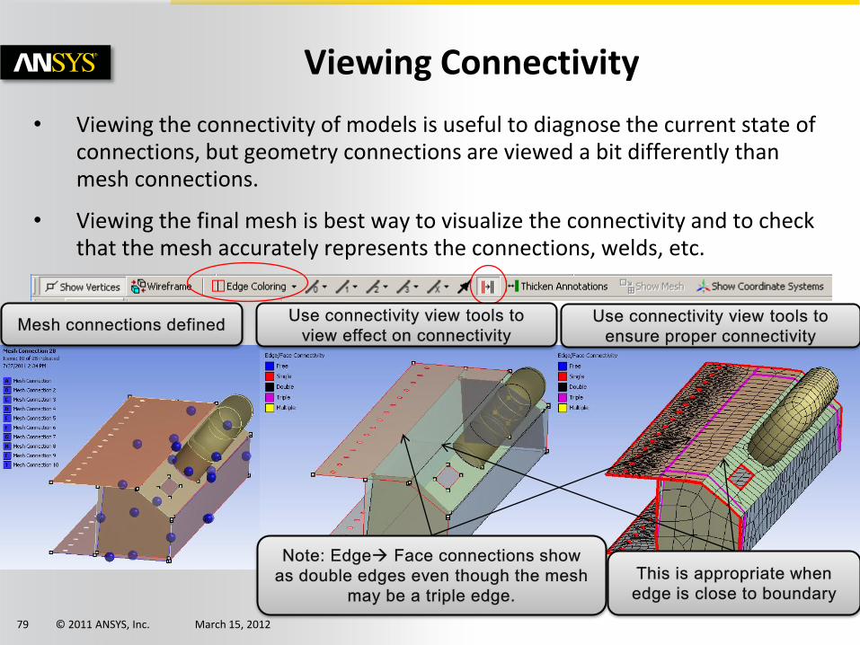
Viewing Connectivity
• Viewing the connectivity of models is useful to diagnose the current state of connections, but geometry connections are viewed a bit differently than mesh connections.
• Viewing the final mesh is best way to visualize the connectivity and to check that the mesh accurately represents the connections, welds, etc.
© 2011 ANSYS, Inc. March 15, 201280
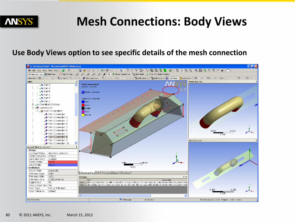
Mesh Connections: Body Views
Use Body Views option to see specific details of the mesh connection
© 2011 ANSYS, Inc. March 15, 201281
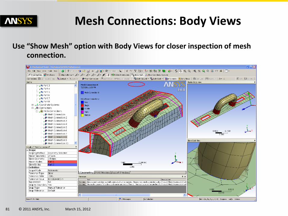
Mesh Connections: Body Views
Use “Show Mesh” option with Body Views for closer inspection of mesh connection.
© 2011 ANSYS, Inc. March 15, 201282
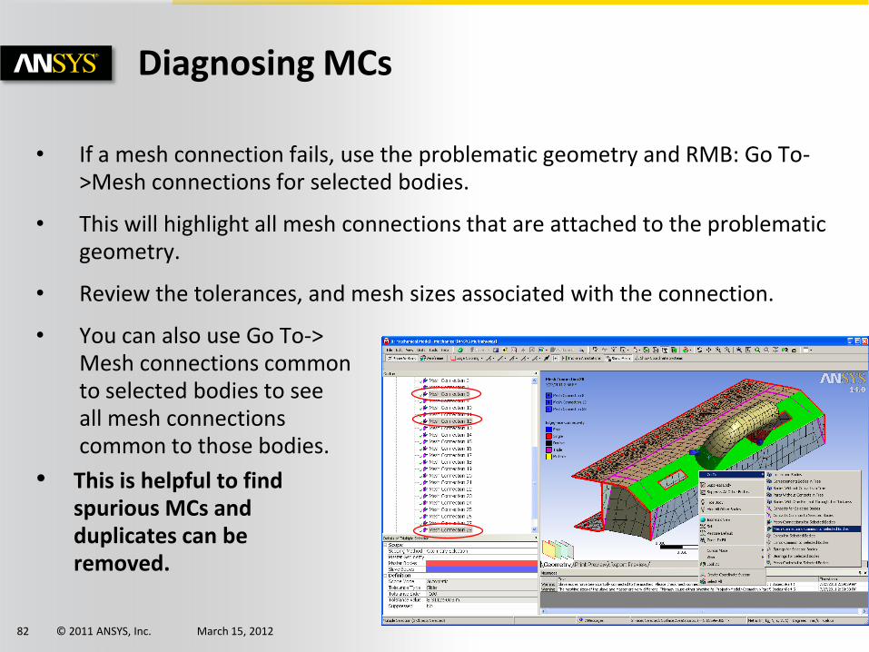
Diagnosing MCs
• If a mesh connection fails, use the problematic geometry and RMB: Go To->Mesh connections for selected bodies.
• This will highlight all mesh connections that are attached to the problematic geometry.
• Review the tolerances, and mesh sizes associated with the connection.
• You can also use Go To->Mesh connections common to selected bodies to see all mesh connections common to those bodies.
• This is helpful to find spurious MCs and duplicates can be removed.

© 2011 ANSYS, Inc. March 15, 201283
14. 0 Release
ANSYS Contact Technology New Features in R14
© 2011 ANSYS, Inc. March 15, 201284
New Features in Rev. 14.0
• Contact Stabilization Damping
• Surface projection based methods
• New “Program Controlled” defaults for Workbench
• Geometry Correction Tools –(for cylinders, spheres, circles)
• Symmetry Conditions for Force Distributed Constraints
© 2011 ANSYS, Inc. March 15, 201285
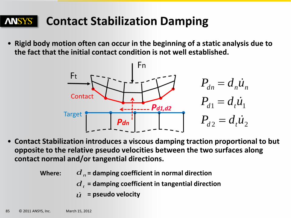
Contact Stabilization Damping
• Rigid body motion often can occur in the beginning of a static analysis due to the fact that the initial contact condition is not well established.
• Contact Stabilization introduces a viscous damping traction proportional to but opposite to the relative pseudo velocities between the two surfaces along contact normal and/or tangential directions.
Where: = damping coefficient in normal direction
= damping coefficient in tangential direction
= pseudo velocity
Fn
Target
Contact
Ft
22
11
udP
udP
udP
td
td
nndn
Pdn
Pd1,d2
u
d
d
t
n
© 2011 ANSYS, Inc. March 15, 201286
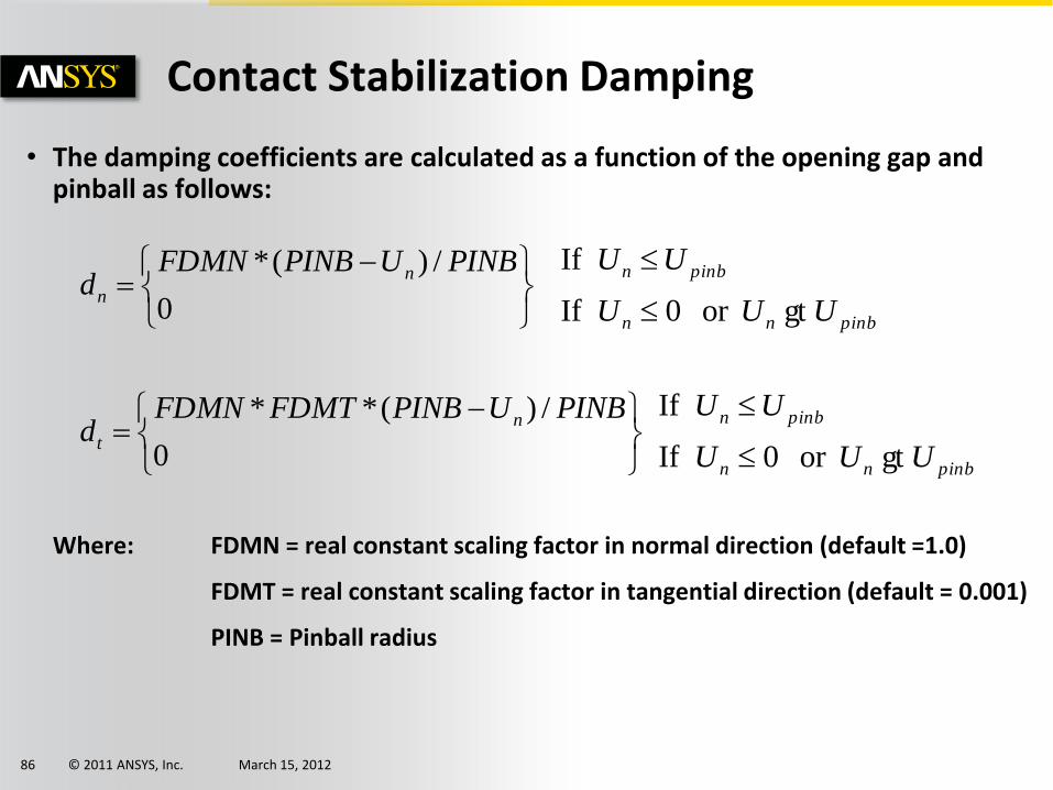
Contact Stabilization Damping
• The damping coefficients are calculated as a function of the opening gap and pinball as follows:
Where: FDMN = real constant scaling factor in normal direction (default =1.0)
FDMT = real constant scaling factor in tangential direction (default = 0.001)
PINB = Pinball radius
0
/)(**
0
/)(*
PINBUPINBFDMTFDMNd
PINBUPINBFDMNd
n
t
n
n
pinbnn
pinbn
UUU
UU
gt or 0 If
If
pinbnn
pinbn
UUU
UU
gt or 0 If
If
© 2011 ANSYS, Inc. March 15, 201287
Contact Stabilization Damping
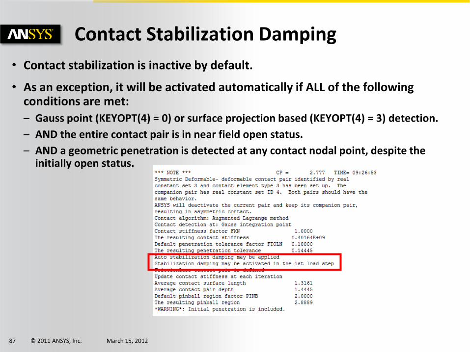
• Contact stabilization is inactive by default.
• As an exception, it will be activated automatically if ALL of the following conditions are met:
– Gauss point (KEYOPT(4) = 0) or surface projection based (KEYOPT(4) = 3) detection.
– AND the entire contact pair is in near field open status.
– AND a geometric penetration is detected at any contact nodal point, despite the initially open status.
© 2011 ANSYS, Inc. March 15, 201288
Contact Stabilization Damping
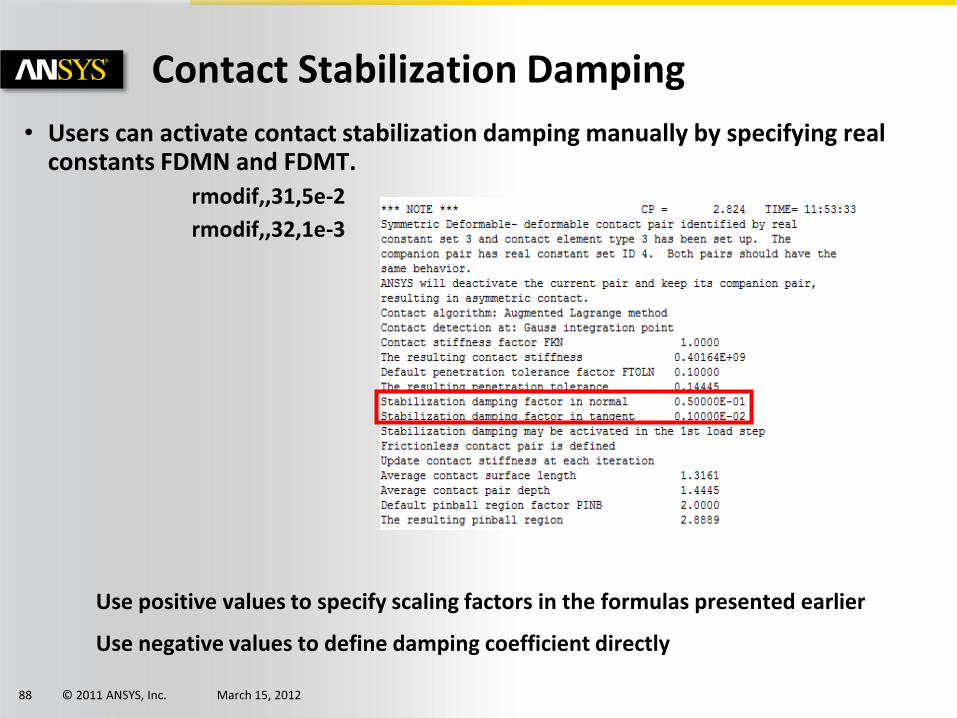
• Users can activate contact stabilization damping manually by specifying real constants FDMN and FDMT.
rmodif,,31,5e-2
rmodif,,32,1e-3
Use positive values to specify scaling factors in the formulas presented earlier
Use negative values to define damping coefficient directly
© 2011 ANSYS, Inc. March 15, 201289
Contact Stabilization Damping
• Additional controls with new KEYOPT(15):
– 0 Damping is activated only in first load step (default)
– 1 Deactivate automatic damping
– 2 Damping is activated for all load steps
– 3 Damping is activated at all times regardless of the contact status of previous steps
• When KEYOPT(15) = 0, 1, or 2, contact stabilization damping will not be applied in the current substep if any contact detection point had a closed status in the previous substep.
• However, when KEYOPT(15) = 3, stabilization damping is always applied as long as the current contact status is near-field open.
© 2011 ANSYS, Inc. March 15, 201290
Contact Stabilization Damping
• Note that the Energy introduced into the model by Contact Stabilization Damping is artificial.
• It can alleviate convergence problems, but it can also affect solution accuracy if the applied stabilization energy generated by the damping forces are too large
– In most cases, the program automatically activates and deactivates contact stabilization damping and estimates reasonable damping forces.
– However, it is a good practice to check the stabilization energy and reaction forces.
• The contact stabilization energy can be post processed via the ETABLE command using the AENE label. This should be compared to element potential energy via SENE label on ETABLE.
For example: ETABLE,AE,AENE !save artificial energies associated with stabilization
ETABLE,SE,SENE !save strain energies to element table
SSUM !sum all element energies for comparison
PRETAB,AE,SE !print element table values
© 2011 ANSYS, Inc. March 15, 201291
Contact Stabilization Damping
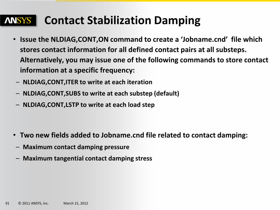
• Issue the NLDIAG,CONT,ON command to create a ‘Jobname.cnd’ file which
stores contact information for all defined contact pairs at all substeps.
Alternatively, you may issue one of the following commands to store contact
information at a specific frequency:
– NLDIAG,CONT,ITER to write at each iteration
– NLDIAG,CONT,SUBS to write at each substep (default)
– NLDIAG,CONT,LSTP to write at each load step
• Two new fields added to Jobname.cnd file related to contact damping:
– Maximum contact damping pressure
– Maximum tangential contact damping stress
© 2011 ANSYS, Inc. March 15, 201292
Contact Stabilization Damping
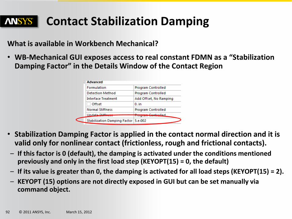
What is available in Workbench Mechanical?
• WB-Mechanical GUI exposes access to real constant FDMN as a “Stabilization Damping Factor” in the Details Window of the Contact Region
• Stabilization Damping Factor is applied in the contact normal direction and it is valid only for nonlinear contact (frictionless, rough and frictional contacts).
– If this factor is 0 (default), the damping is activated under the conditions mentioned previously and only in the first load step (KEYOPT(15) = 0, the default)
– If its value is greater than 0, the damping is activated for all load steps (KEYOPT(15) = 2).
– KEYOPT (15) options are not directly exposed in GUI but can be set manually via command object.
© 2011 ANSYS, Inc. March 15, 201293
Contact Stabilization Damping
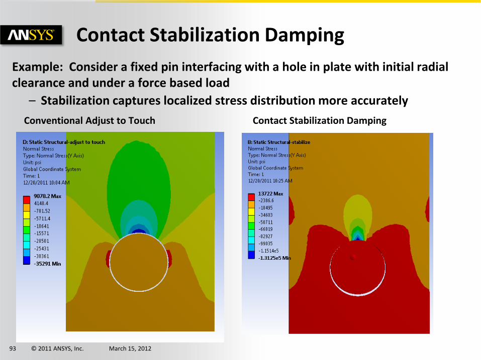
Example: Consider a fixed pin interfacing with a hole in plate with initial radialclearance and under a force based load
– Stabilization captures localized stress distribution more accurately
Conventional Adjust to Touch Contact Stabilization Damping
© 2011 ANSYS, Inc. March 15, 201294
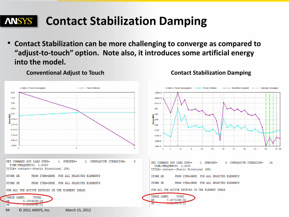
Contact Stabilization Damping
• Contact Stabilization can be more challenging to converge as compared to “adjust-to-touch” option. Note also, it introduces some artificial energy into the model.
Conventional Adjust to Touch Contact Stabilization Damping
© 2011 ANSYS, Inc. March 15, 201295
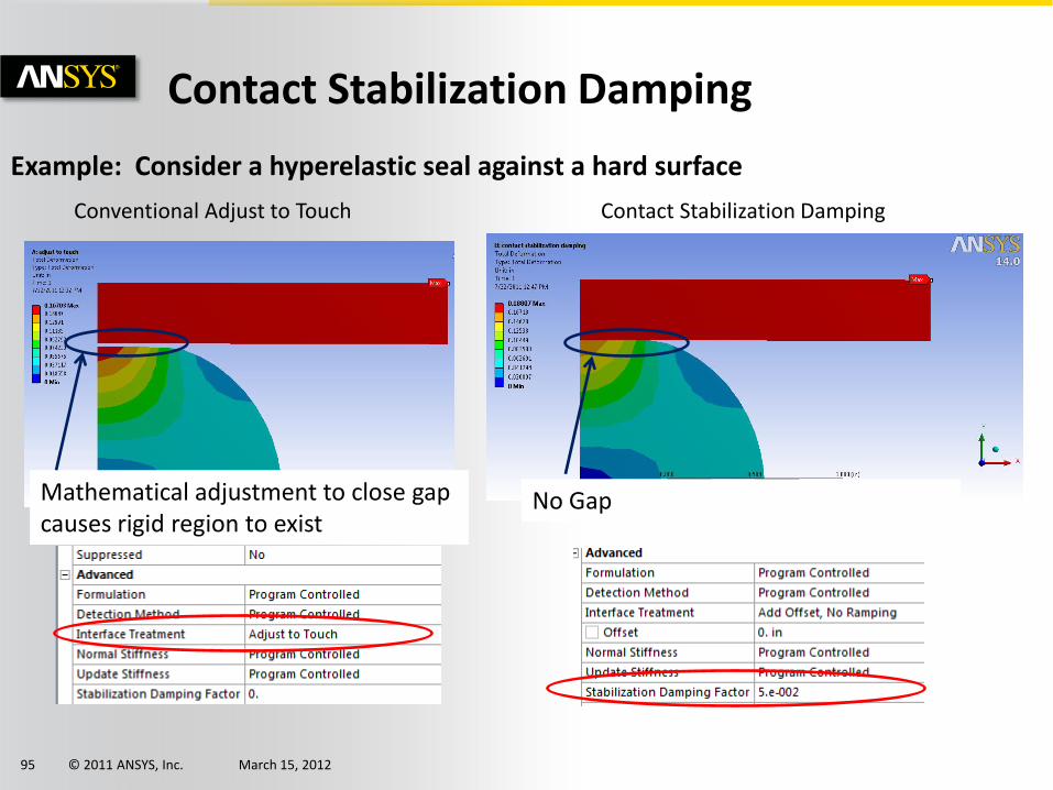
Contact Stabilization Damping
Mathematical adjustment to close gap causes rigid region to exist
No Gap
Conventional Adjust to Touch Contact Stabilization Damping
Example: Consider a hyperelastic seal against a hard surface
© 2011 ANSYS, Inc. March 15, 201296
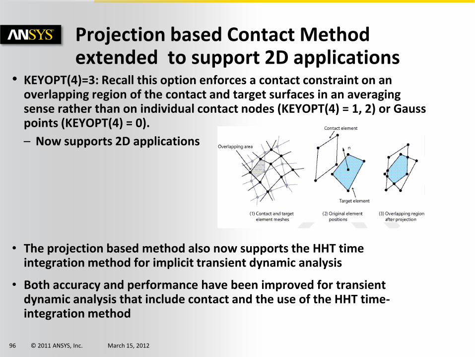
Projection based Contact Method extended to support 2D applications
• KEYOPT(4)=3: Recall this option enforces a contact constraint on an overlapping region of the contact and target surfaces in an averaging sense rather than on individual contact nodes (KEYOPT(4) = 1, 2) or Gauss points (KEYOPT(4) = 0).
– Now supports 2D applications
• The projection based method also now supports the HHT time integration method for implicit transient dynamic analysis
• Both accuracy and performance have been improved for transient dynamic analysis that include contact and the use of the HHT time-integration method
© 2011 ANSYS, Inc. March 15, 201297
Projection Based Method
Advantages over conventional detection methods• Less sensitive to the designation of contact and target surfaces
• In general, it provides more accurate contact results.
– Stress distribution across contacting interface is smoother.
• It meets moment equilibrium even when offset exists between contact and target surfaces with friction.
• Contact forces do not jump when contact nodes slide off the edge of target surface
Disadvantages:
• Computationally more expensive
• When a model has corner or edge contact, the averaged penetration/gap could be quite different than the real geometric penetration observed at contact nodes.
– In this situation, mesh refinement is usually required.
© 2011 ANSYS, Inc. March 15, 201298
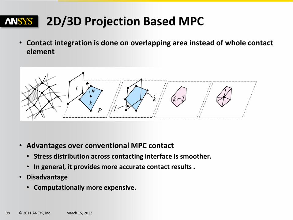
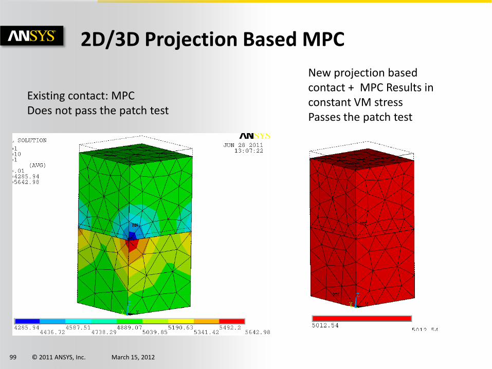
2D/3D Projection Based MPC
• Contact integration is done on overlapping area instead of whole contact element
• Advantages over conventional MPC contact
• Stress distribution across contacting interface is smoother.
• In general, it provides more accurate contact results .
• Disadvantage
• Computationally more expensive.
© 2011 ANSYS, Inc. March 15, 201299
Existing contact: MPCDoes not pass the patch test
New projection based contact + MPC Results in constant VM stressPasses the patch test
2D/3D Projection Based MPC
© 2011 ANSYS, Inc. March 15, 2012100
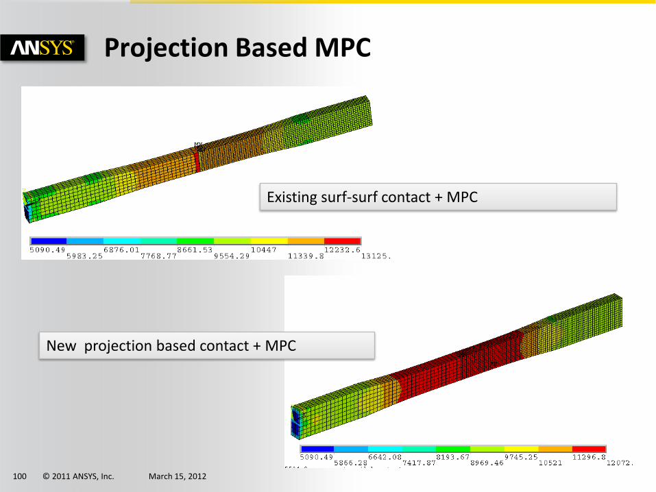
Projection Based MPC
Existing surf-surf contact + MPC
New projection based contact + MPC
© 2011 ANSYS, Inc. March 15, 2012101
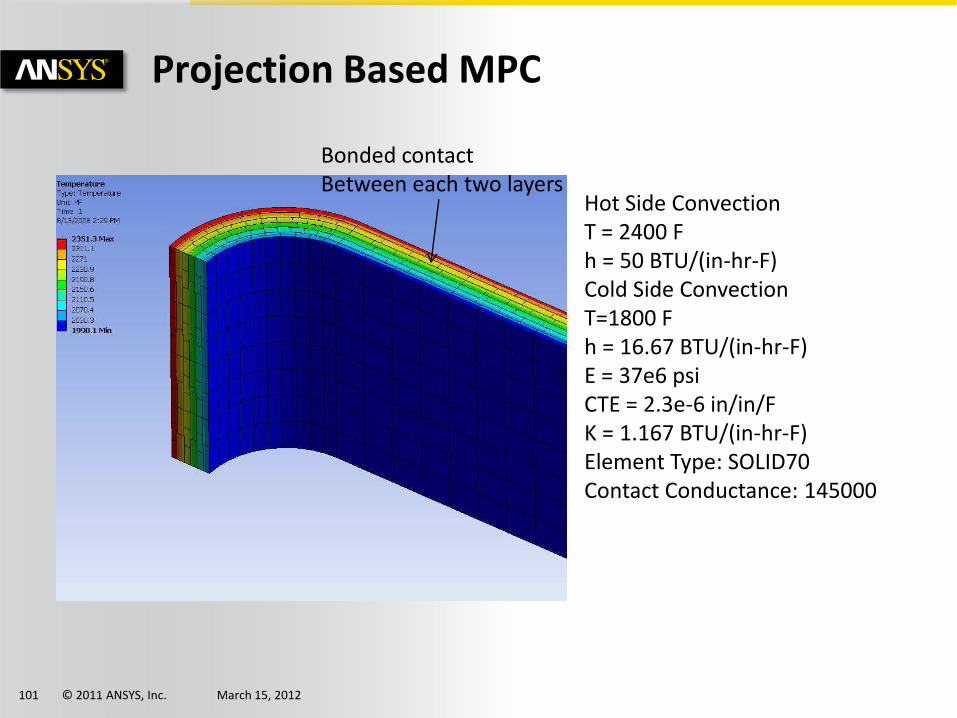
Projection Based MPC
Hot Side ConvectionT = 2400 Fh = 50 BTU/(in-hr-F)Cold Side ConvectionT=1800 Fh = 16.67 BTU/(in-hr-F)E = 37e6 psiCTE = 2.3e-6 in/in/FK = 1.167 BTU/(in-hr-F)Element Type: SOLID70Contact Conductance: 145000
Bonded contact Between each two layers
© 2011 ANSYS, Inc. March 15, 2012102
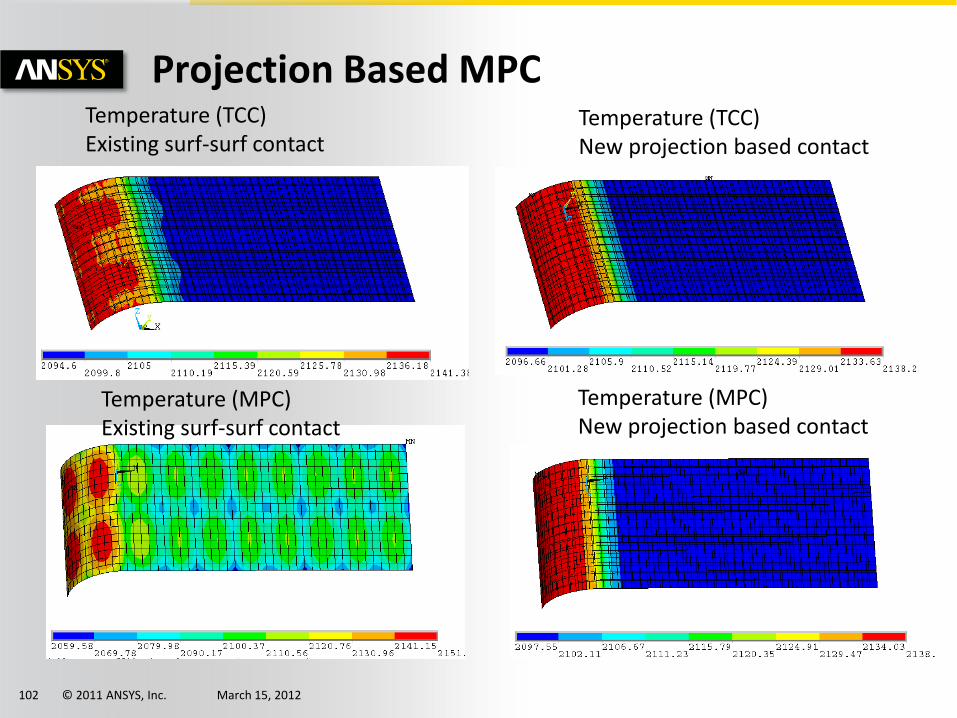
Projection Based MPCTemperature (TCC)Existing surf-surf contact
Temperature (TCC)New projection based contact
Temperature (MPC)New projection based contact
Temperature (MPC)Existing surf-surf contact
© 2011 ANSYS, Inc. March 15, 2012103
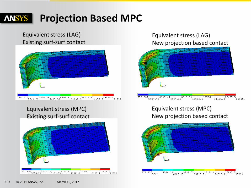
Projection Based MPC
Equivalent stress (LAG)Existing surf-surf contact
Equivalent stress (MPC)Existing surf-surf contact
Equivalent stress (LAG)New projection based contact
Equivalent stress (MPC)New projection based contact
© 2011 ANSYS, Inc. March 15, 2012104
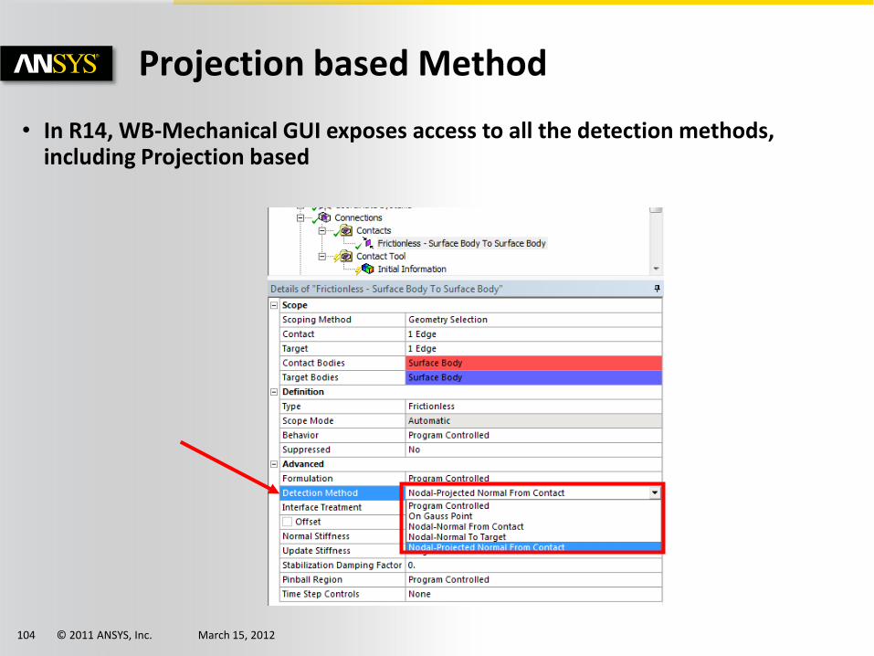
Projection based Method
• In R14, WB-Mechanical GUI exposes access to all the detection methods, including Projection based
© 2011 ANSYS, Inc. March 15, 2012105
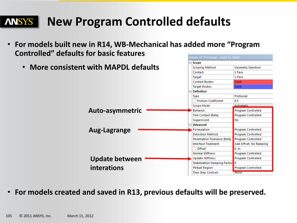
• For models built new in R14, WB-Mechanical has added more “Program Controlled” defaults for basic features
• More consistent with MAPDL defaults
• For models created and saved in R13, previous defaults will be preserved.
New Program Controlled defaults
Aug-Lagrange
Auto-asymmetric
Update between interations
© 2011 ANSYS, Inc. March 15, 2012106
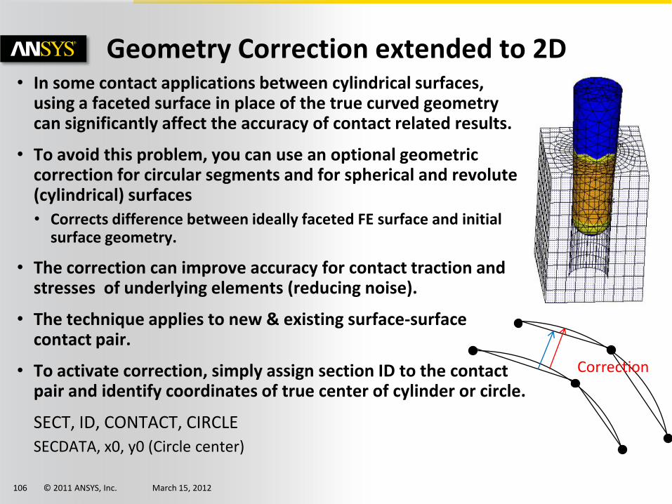
Geometry Correction extended to 2D • In some contact applications between cylindrical surfaces,
using a faceted surface in place of the true curved geometry can significantly affect the accuracy of contact related results.
• To avoid this problem, you can use an optional geometric correction for circular segments and for spherical and revolute (cylindrical) surfaces
• Corrects difference between ideally faceted FE surface and initial surface geometry.
• The correction can improve accuracy for contact traction and stresses of underlying elements (reducing noise).
• The technique applies to new & existing surface-surface contact pair.
• To activate correction, simply assign section ID to the contact pair and identify coordinates of true center of cylinder or circle.
SECT, ID, CONTACT, CIRCLE
SECDATA, x0, y0 (Circle center)
Correction
© 2011 ANSYS, Inc. March 15, 2012107
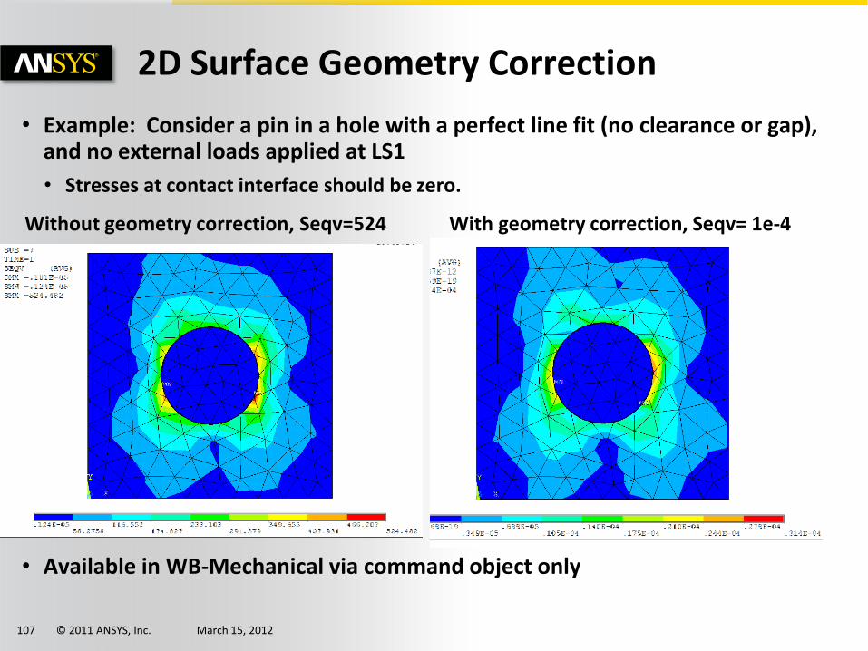
• Example: Consider a pin in a hole with a perfect line fit (no clearance or gap), and no external loads applied at LS1
• Stresses at contact interface should be zero.
Without geometry correction, Seqv=524 With geometry correction, Seqv= 1e-4
• Available in WB-Mechanical via command object only
2D Surface Geometry Correction
© 2011 ANSYS, Inc. March 15, 2012108
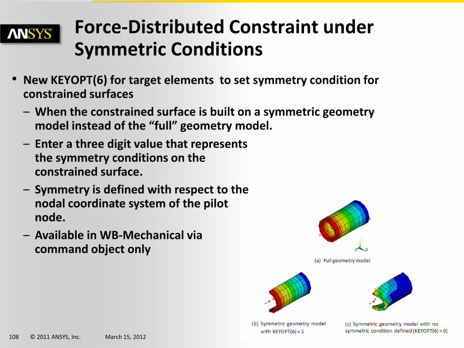
Force-Distributed Constraint under Symmetric Conditions
• New KEYOPT(6) for target elements to set symmetry condition for constrained surfaces
– When the constrained surface is built on a symmetric geometry model instead of the “full” geometry model.
– Enter a three digit value that represents the symmetry conditions on the constrained surface.
– Symmetry is defined with respect to the nodal coordinate system of the pilot node.
– Available in WB-Mechanical via command object only
© 2011 ANSYS, Inc. March 15, 2012109
Critical Temperature for Bonding
• After materials around contacting surfaces exceed a critical temperature, the surfaces start to melt and bond with each other.
• The critical temperature is defined by the new TBND real constant on the contact elements.
• As soon as the temperature at the contact surface exceeds this melting temperature, the contact will change to “bonded” and will remain bonded for the rest of the analysis.
• Available in WB-Mechanical via command object only
© 2011 ANSYS, Inc. March 15, 2012110
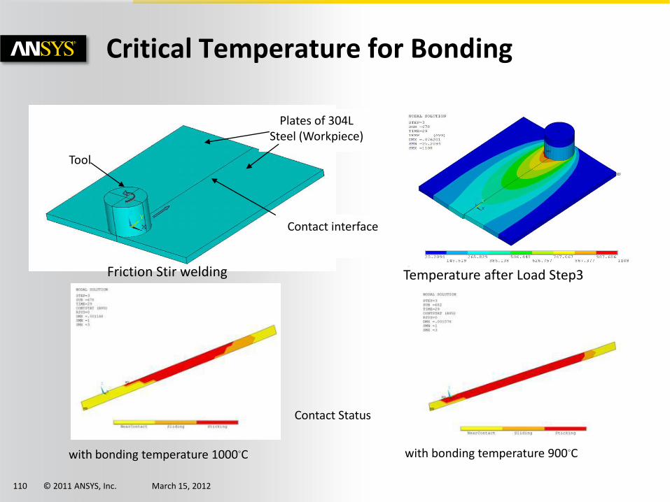
Critical Temperature for Bonding
Tool
Plates of 304L Steel (Workpiece)
Contact interface
Temperature after Load Step3Friction Stir welding
with bonding temperature 1000◦C with bonding temperature 900◦C
Contact Status
© 2011 ANSYS, Inc. March 15, 2012111
Advanced Modeling
Offshore Structures
© 2011 ANSYS, Inc. March 15, 2012112
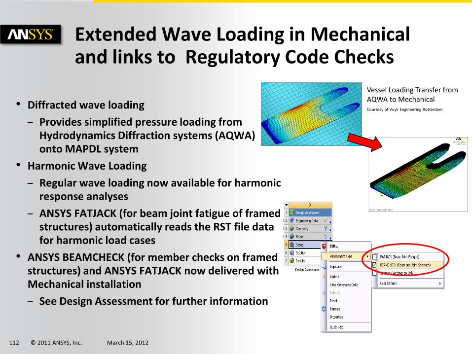
• Diffracted wave loading
– Provides simplified pressure loading from Hydrodynamics Diffraction systems (AQWA) onto MAPDL system
• Harmonic Wave Loading
– Regular wave loading now available for harmonic response analyses
– ANSYS FATJACK (for beam joint fatigue of framed structures) automatically reads the RST file data for harmonic load cases
• ANSYS BEAMCHECK (for member checks on framed structures) and ANSYS FATJACK now delivered with Mechanical installation
– See Design Assessment for further information
Extended Wave Loading in Mechanical and links to Regulatory Code Checks
Vessel Loading Transfer from AQWA to MechanicalCourtesy of Vuyk Engineering Rotterdam
© 2011 ANSYS, Inc. March 15, 2012113
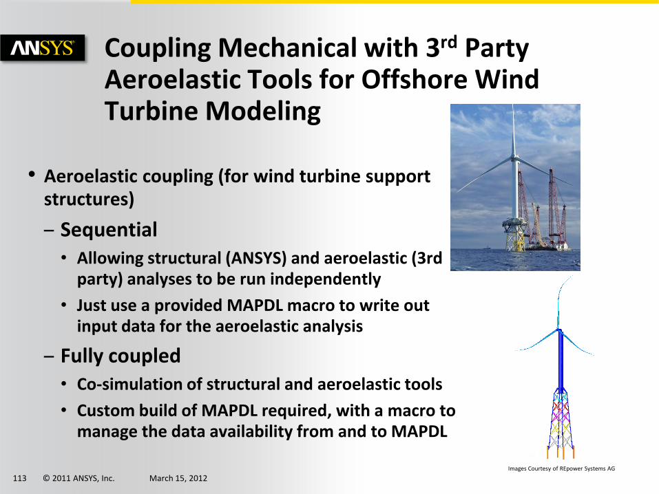
• Aeroelastic coupling (for wind turbine support structures)
– Sequential • Allowing structural (ANSYS) and aeroelastic (3rd
party) analyses to be run independently
• Just use a provided MAPDL macro to write out input data for the aeroelastic analysis
– Fully coupled • Co-simulation of structural and aeroelastic tools
• Custom build of MAPDL required, with a macro to manage the data availability from and to MAPDL
Coupling Mechanical with 3rd Party Aeroelastic Tools for Offshore Wind Turbine Modeling
Images Courtesy of REpower Systems AG
© 2011 ANSYS, Inc. March 15, 2012114
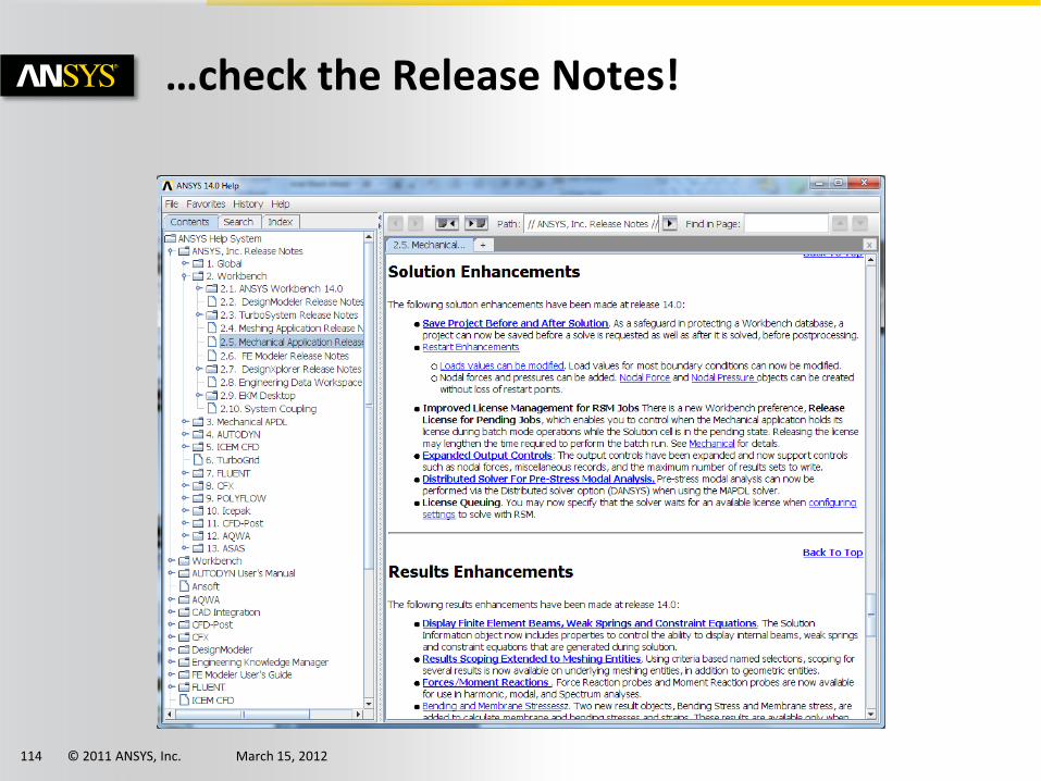
…check the Release Notes!
© 2011 ANSYS, Inc. March 15, 2012115
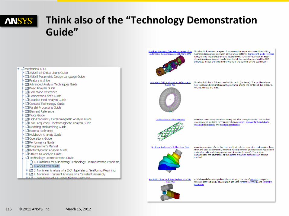
Think also of the “Technology Demonstration Guide”

© 2011 ANSYS, Inc. March 15, 2012116
THANK YOU
Recommended