[Type text]
Improving Durability TSCS – Measuring Asphalt Density
November 2016
Project No: 60484596
Prepared for: Highways England
Prepared by: AECOM
AECOM Infrastructure & Environment UK Limited 12 Regan Way, Chetwyn Business Park, Nottingham NG9 6RZ Tel +44 (0) 115 9077000 Fax +44 (0) 115 9077001

IMPROVING DURABILITY TSCS – MEASURING ASPHALT DENSITY
60484596
November 2016
i
REVISION SCHEDULE:
REV DATE DETAILS PREPARED BY REVIEWED BY APPROVED BY
1 November 2016
Final Report for Comment
Yi Xu
Senior Assistant Engineer
Jack Bull
Technical Director
Sam Nicklin
Assistant Engineer
Daru Widyatmoko
Technical Director
IMPROVING DURABILITY TSCS – MEASURING ASPHALT DENSITY
60484596
November 2016
ii
Limitations
AECOM through its subsidiary URS Infrastructure & Environment UK Limited (hereafter referred to as
“AECOM”) has prepared this Report for the sole use of Highways England (“Client”) in accordance with the
Agreement under which our services were performed. No other warranty, expressed or implied, is made as
to the professional advice included in this Report or any other services provided by AECOM. This Report is
confidential and may not be disclosed by the Client nor relied upon by any other party without the prior and
express written agreement of AECOM.
The conclusions and recommendations contained in this Report are based upon information provided by
others and upon the assumption that all relevant information has been provided by those parties from whom
it has been requested and that such information is accurate. Information obtained by URS has not been
independently verified by AECOM, unless otherwise stated in the Report.
The methodology adopted and the sources of information used by AECOM in providing its services are
outlined in this Report. The work described in this Report was undertaken in February to November 2016
and is based on the conditions encountered and the information available during the said period of time. The
scope of this Report and the services are accordingly factually limited by these circumstances.
Where assessments of works or costs identified in this Report are made, such assessments are based upon
the information available at the time and where appropriate are subject to further investigations or
information which may become available.
AECOM disclaim any undertaking or obligation to advise any person of any change in any matter affecting
the Report, which may come or be brought to AECOM’s attention after the date of the Report.
Certain statements made in the Report that are not historical facts may constitute estimates, projections or
other forward-looking statements and even though they are based on reasonable assumptions as of the date
of the Report, such forward-looking statements by their nature involve risks and uncertainties that could
cause actual results to differ materially from the results predicted. AECOM specifically does not guarantee or
warrant any estimate or projections contained in this Report.
Where field investigations are carried out, these have been restricted to a level of detail required to meet the
stated objectives of the services. The results of any measurements taken may vary spatially or with time and
further confirmatory measurements should be made after any significant delay in issuing this Report.
Copyright
© This Report is the copyright of AECOM Infrastructure & Environment UK Limited. Any unauthorised
reproduction or usage by any person other than the addressee is strictly prohibited.
IMPROVING DURABILITY TSCS – MEASURING ASPHALT DENSITY
60484596
November 2016
iii
TABLE OF CONTENTS 1. INTRODUCTION ............................................................... 1
1.1. Background ........................................................................ 1
1.2. Compaction and Density of Hot Mix Asphalt ..................... 2
1.3. Objective and Scope .......................................................... 3
1.4. Report Outline .................................................................... 3
2. DENSITY MEASUREMENT – COMMON METHODS ...... 3
2.1. Core Method ...................................................................... 3
2.2. Nuclear Density Gauge (NDG) .......................................... 5
3. DENSITY MEASUREMENT– OTHER METHODS ......... 15
3.1. Capacitive Electromagnetic Method – PQI & PaveTracker15
3.2. Electromagnetic Wave-Based Method – Radar Systems 24
3.3. Ultrasound Method........................................................... 29
3.4. Roller Mounted Asphalt Density Devices ........................ 29
4. RECOMMENDATIONS ................................................... 31
5. TESTING ......................................................................... 34
5.1. Laboratory Large scale Pavement Trials ......................... 34
5.2. Materials .......................................................................... 36
5.3. Devices ............................................................................ 36
5.4. Basic Data ........................................................................ 38
5.5. Calibration ........................................................................ 39
6. ANALYSIS ....................................................................... 47
6.1. Regression Analysis ........................................................ 47
6.2. PQI Density Regression Analysis .................................... 47
6.3. NDG Density Regression Analysis .................................. 49
6.4. Measurement errors......................................................... 51
6.5. Gage R&R Study – Nested ANOVA ................................ 52
7. CONCLUSIONS AND RECOMMENDATIONS ............... 57
7.1. Conclusions ..................................................................... 57
7.2. Reccomendations ............................................................ 58
8. REFERENCES ................................................................ 59
IMPROVING DURABILITY TSCS – MEASURING ASPHALT DENSITY
60484596
November 2016
1
1. INTRODUCTION
1.1. BACKGROUND
The high level objectives of the Agency are value for money, driving innovation and improving
efficiency. The Agency has a range of intrusive and non-intrusive pavement investigation
techniques that are employed to assess the condition of the network, to evaluate safety critical
performance and the pavement’s structural capacity.
Thin surface Course Systems (TSCS) are asphalt materials that are safe to drive on, easy to install
and help to reduce road traffic noise. They were originally developed in France and Germany and
were introduced on UK roads in the late 1990’s. Previous research has shown that these materials
can last for up to 16 years, even on roads with very high traffic levels. However, recent harsh
winters have led to some road surfaces deteriorating prematurely and very rapidly. Like many
organic substances, bitumen slowly oxidises when in contact with air. The degree of oxidation
(often simply referred as “ageing”) is highly dependent on the temperature, time and the thickness
of the bitumen film. It is recognised that over time, asphalt ageing can lead to pothole formation.
There is a view that density, air voids and binder content have a significant role on the in situ
performance of road surfacings, and ultimately TSCS service life. A detailed study to investigate
the possible testing methods for measuring TSCS in situ air voids and to develop a most suitable
method for these systems is therefore considered important.
This project forms part of a wider Highways England strategy to develop value for money surfacing
materials and treatments for the strategic road network that are safe and durable, whilst minimising
road traffic noise and embodied carbon. Previous research reports have shown that thin surfacings
can deliver equivalent whole life cost benefits to traditional surfacings but with the added benefit of
reducing traffic noise.
The primary objective of this project is to ensure that asphalt surfacings continue to deliver value
for money on the strategic road network and to maximise the benefit from innovation.
On 6 January 2016, AECOM (formerly URS) was commissioned by Highways England to carry out
a study on “Improving Durability of TSCS”, under the Framework for Transport Related Technical
and Engineering Advice and Research –Package Order Ref: 671(4/45/12)ARPS. The project aims
to develop a non-destructive test method to assess in situ density of asphalt surfacing. This work
has been divided into the following sub-tasks:
IMPROVING DURABILITY TSCS – MEASURING ASPHALT DENSITY
60484596
November 2016
2
1. Complete a literature study on the testing methods available worldwide for measuring TSCS
density. To shortlist the most suitable options and complete trials for each option.
2. To develop a practical method for measuring TSCS density in-situ.
This report presents findings from the literature study and discusses the suitability of current non-
destructive density testing equipment.
1.2. COMPACTION AND DENSITY OF HOT MIX ASPHALT
Compaction is essential in the construction of hot mix asphalt (HMA) to ensure long-term durability.
For base and binder course, the compaction level is monitored and controlled by the in-situ void
content specified in Manual of Contract Document for Highway Works, Volume 1, (MCHW 1)
Clauses 929, 930 and 937. However currently there is no such requirement specified for TSCS.
Void content that is either too high or too low can lead to premature failure. A pavement with a high
void content as a result of poor compaction is prone to water penetration and defects such as
cracking and ravelling. On the other hand, a pavement with very low void content may lead to
rutting and shoving (Brown 1990). A general threshold value of 7% applies for a newly constructed
asphalt concrete dense base and binder course (MCHW 1 Clause 929). However no threshold
currently applies to TSCS. The void content is determined in accordance with BS EN 12697-8
using the bulk density and the maximum density according to BS EN 12697 – 6 and 5 respectively.
Due to the nature of the composite mixture material, as Romero (2002) states “no absolute density
value can be defined and some variations in density measurements exist”. Two commonly used
methods of measuring in situ asphalt bulk density are core and nuclear density gauge (NDG). The
former requires extraction of core samples for further laboratory assessments. It is the only direct
measurement of the asphalt density but has drawbacks of increased time and cost needed from
core extraction to the end of testing is time-consuming and costly. The NDG is a quick and non-
destructive alternative solution, but has practical limitations and health and safety risks due to its
use of radioactive material. There are also stringent requirements on store, transport and use of
the NDG and training and licensing of the operatives. Hence, there was a need to replace NDG
with safer and easier-to-operate equipment. Furthermore the effectiveness of NDG to determine in
situ density of thin asphalt layers (such as TSCS) is unknown.
Electromagnetic devices for HMA density measurements were made commercially available in the
late 1990s. They are non-radioactive, light-weight, safe, easy to use and can provide rapid and
reliable readings. Many studies on the electromagnetic devices have been published in the last 15
years in the United States, which recommended these devices were “at least as good as nuclear
IMPROVING DURABILITY TSCS – MEASURING ASPHALT DENSITY
60484596
November 2016
3
density gauges” (Williams et al 2007). Nevertheless, there are conflicting views on the application
of these devices including whether they should be used to provide density values (referred to as
“Quality Assurance”) or to provide density changes only (referred to as “Quality Control”). Other
technologies, which are claimed to be successful alternatives for measuring in-situ asphalt
densities, are also introduced in this report. However, many of these are still at the research stage
and not commercially available.
1.3. OBJECTIVE AND SCOPE
The primary objective of this research is to review and evaluate the available methods of
measuring the density of hot mix asphalt (HMA) pavements, with a specific interest on thin asphalt
layers in the range of 30mm to 50mm. Non-destructive methods using NDG, electromagnetic
instruments and other techniques, such as ground-penetrating radar, step frequency radar and the
newly-developed compacting monitoring system are compared with the conventional coring
method. The advantages and limitations of these methods are examined. Furthermore, some
national and international cases are studied to collate lessons and compare different technologies.
Some technologies are still at the research stage and in need of further development before they
can be adopted by the industry. They are briefly introduced in the review to demonstrate possible
future developments. However, more emphasis is given to the established technologies which
could be more readily applied.
1.4. REPORT OUTLINE
The common methods for measuring asphalt density - core method and NDG method are
described in Section 2. Section 3 summarises other non-destructive methods including capacitive
electromagnetic devices, the electromagnetic wave-based methods, ultrasound technology and the
recent development of compaction monitoring systems. All these density measurement methods
are evaluated by their attributes, on basis of which recommendations are given in Section 4.
Section 5 discusses the testing completed based on Section 4 recommendations and Section 6
presents results and analysis for testing completed at AECOM Nottingham’s Test Pit Facility.
2. DENSITY MEASUREMENT – COMMON METHODS
2.1. CORE METHOD
Although the core method is costly and time-consuming it is still widely used. Intrusive coring and
reinstatement creates a local weakness in the pavement which can fail later on. Nevertheless, the
core method is the only direct measurement of the density and still plays an important role for
calibrating other methods.
IMPROVING DURABILITY TSCS – MEASURING ASPHALT DENSITY
60484596
November 2016
4
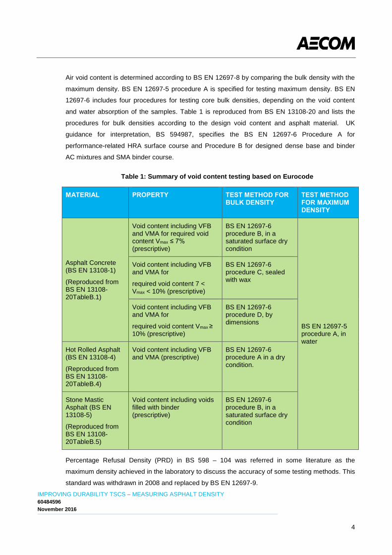
Air void content is determined according to BS EN 12697-8 by comparing the bulk density with the
maximum density. BS EN 12697-5 procedure A is specified for testing maximum density. BS EN
12697-6 includes four procedures for testing core bulk densities, depending on the void content
and water absorption of the samples. Table 1 is reproduced from BS EN 13108-20 and lists the
procedures for bulk densities according to the design void content and asphalt material. UK
guidance for interpretation, BS 594987, specifies the BS EN 12697-6 Procedure A for
performance-related HRA surface course and Procedure B for designed dense base and binder
AC mixtures and SMA binder course.
Table 1: Summary of void content testing based on Eurocode
MATERIAL PROPERTY TEST METHOD FOR BULK DENSITY
TEST METHOD FOR MAXIMUM DENSITY
Asphalt Concrete (BS EN 13108-1)
(Reproduced from BS EN 13108-20TableB.1)
Void content including VFB and VMA for required void content Vmax ≤ 7% (prescriptive)
BS EN 12697-6 procedure B, in a saturated surface dry condition
BS EN 12697-5 procedure A, in water
Void content including VFB and VMA for
required void content 7 < Vmax < 10% (prescriptive)
BS EN 12697-6 procedure C, sealed with wax
Void content including VFB and VMA for
required void content Vmax ≥ 10% (prescriptive)
BS EN 12697-6 procedure D, by dimensions
Hot Rolled Asphalt (BS EN 13108-4)
(Reproduced from BS EN 13108-20TableB.4)
Void content including VFB and VMA (prescriptive)
BS EN 12697-6 procedure A in a dry condition.
Stone Mastic Asphalt (BS EN 13108-5)
(Reproduced from BS EN 13108-20TableB.5)
Void content including voids filled with binder (prescriptive)
BS EN 12697-6 procedure B, in a saturated surface dry condition
Percentage Refusal Density (PRD) in BS 598 – 104 was referred in some literature as the
maximum density achieved in the laboratory to discuss the accuracy of some testing methods. This
standard was withdrawn in 2008 and replaced by BS EN 12697-9.
IMPROVING DURABILITY TSCS – MEASURING ASPHALT DENSITY
60484596
November 2016
5
Maximum theoretical density (MTD) or “Rice” density, is another important referencing density. It is
based on the proportions and densities of aggregate and binder in the mixture. This is explained in
the EN 12697-5 procedure C mathematical procedure.
2.2. NUCLEAR DENSITY GAUGE (NDG)
2.2.1. HISTORY
The first documented NDG use for measuring asphalt density was published in a conference in
Chicago (Stephens 1964). The American Society for Testing and Materials (ASTM) developed
standard D2950 in 1971 for testing asphalt densities using nuclear density gauges. It has
incorporated a number of changes since, such as the addition of the precision and bias statement
in the 2011 version (ASTM Committee D04.21, 2009). The latest version was published in 2014.
In the UK, the core method has been the dominant method of measuring asphalt density until
1982, when an official evaluation report on NDG was published by the Transport Research
Laboratory (TRL). A working party was set up to assess and compare the NDG with traditional
coring method in six motorway reconstruction contracts. The Campbell-Pacific MC-2 type NDG
was used to measure densities adjacent to the core positions. Compliance checks using cores and
NDG reached the same conclusion in 84% of the results. However, it was also recommended that
coring shall be used to calibrate gauge measurements if in doubt. Comparative tests revealed that
NDG readings were more variable than core densities. The gauge calibration temperature on the
gauge calibration was reported to have minor impact on the readings along with the moisture
condition of pavement surface. Overall, it was recognised that NDG could reduce the volume of
testing on site and was a “simple, quick and non-destructive alternative method for measuring
density” (TRRL 1982). This document also provided a procedure for using NDG. NDG was added
to the later-published BS 4987:1988 as an alternative method for compliance checking on asphalt
compaction. This served as relative readings compared to 93% PRD. This standard was replaced
by BS 594987 in 2007 which included the informative protocol on calibration and operation.
2.2.2. COMPTON EFFECT AND NDG MODES
NDG works using the “Compton Effect”, also referred to as “Compton Scatter”. It is defined as “the
scattering and increase in wavelength of an X-ray (or gamma-ray) photon on encountering an
electron, with a partial transference of energy from the photon to the electron.” (Oxford English
Dictionary online, 2016). Briefly, a small gamma ray is emitted from a radioactive source,
transmitted through the pavement material and counted by the detector(s) on the other side of the
NDG. The denser the pavement, the more energy consumed in penetrating the material and the
count number. Conversely, a less well compacted pavement will be penetrated through more
IMPROVING DURABILITY TSCS – MEASURING ASPHALT DENSITY
60484596
November 2016
6
easily so has a higher count reading. A direct correlation between the photon count and the
material density can be therefore estimated (Troxler 2007).
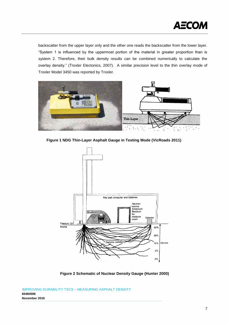
There are two main testing modes – the backscatter mode and the direct transmission mode. The
former is a non-destructive testing mode which measures density in layer thicknesses up to
100mm (see Figure 1). It comprises a radioactive source and two detectors, one at the centre and
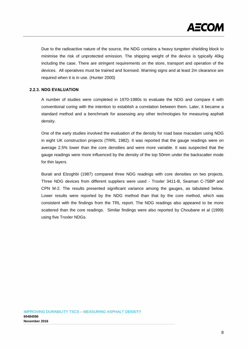
a second at one end. The latter incorporates an extendable source rod, which is placed through a
pre-drilled hole to 300mm deep (see Figure 2). The density of the material up to 300mm thick can
be measured. The testing mode “thin lift”, uses the same approach as the conventional back-
scatter mode but with different algorithm to account for the mat thickness. It is designed to
measure the density of thin layers from 25 to 100 mm. It is available on some newer models, such
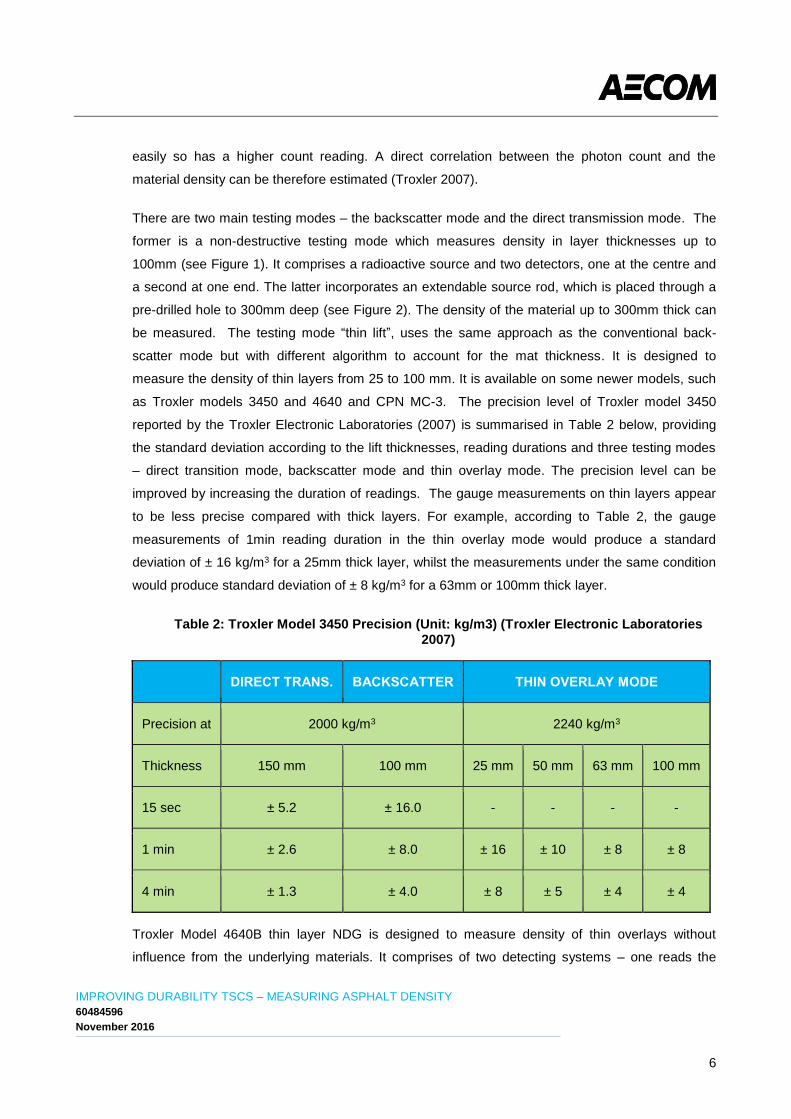
as Troxler models 3450 and 4640 and CPN MC-3. The precision level of Troxler model 3450
reported by the Troxler Electronic Laboratories (2007) is summarised in Table 2 below, providing
the standard deviation according to the lift thicknesses, reading durations and three testing modes
– direct transition mode, backscatter mode and thin overlay mode. The precision level can be
improved by increasing the duration of readings. The gauge measurements on thin layers appear
to be less precise compared with thick layers. For example, according to Table 2, the gauge
measurements of 1min reading duration in the thin overlay mode would produce a standard
deviation of ± 16 kg/m3 for a 25mm thick layer, whilst the measurements under the same condition
would produce standard deviation of ± 8 kg/m3 for a 63mm or 100mm thick layer.
Table 2: Troxler Model 3450 Precision (Unit: kg/m3) (Troxler Electronic Laboratories 2007)
DIRECT TRANS. BACKSCATTER THIN OVERLAY MODE
Precision at 2000 kg/m3 2240 kg/m3
Thickness 150 mm 100 mm 25 mm 50 mm 63 mm 100 mm
15 sec ± 5.2 ± 16.0 - - - -
1 min ± 2.6 ± 8.0 ± 16 ± 10 ± 8 ± 8
4 min ± 1.3 ± 4.0 ± 8 ± 5 ± 4 ± 4
Troxler Model 4640B thin layer NDG is designed to measure density of thin overlays without
influence from the underlying materials. It comprises of two detecting systems – one reads the
IMPROVING DURABILITY TSCS – MEASURING ASPHALT DENSITY
60484596
November 2016
7
backscatter from the upper layer only and the other one reads the backscatter from the lower layer.
“System 1 is influenced by the uppermost portion of the material in greater proportion than is
system 2. Therefore, their bulk density results can be combined numerically to calculate the
overlay density.” (Troxler Electonics, 2007). A similar precision level to the thin overlay mode of
Troxler Model 3450 was reported by Troxler.
Figure 1 NDG Thin-Layer Asphalt Gauge in Testing Mode (VicRoads 2011)
Figure 2 Schematic of Nuclear Density Gauge (Hunter 2000)
IMPROVING DURABILITY TSCS – MEASURING ASPHALT DENSITY
60484596
November 2016
8
Due to the radioactive nature of the source, the NDG contains a heavy tungsten shielding block to
minimise the risk of unprotected emission. The shipping weight of the device is typically 40kg
including the case. There are stringent requirements on the store, transport and operation of the
devices. All operatives must be trained and licensed. Warning signs and at least 2m clearance are
required when it is in use. (Hunter 2000)
2.2.3. NDG EVALUATION
A number of studies were completed in 1970-1980s to evaluate the NDG and compare it with
conventional coring with the intention to establish a correlation between them. Later, it became a
standard method and a benchmark for assessing any other technologies for measuring asphalt
density.
One of the early studies involved the evaluation of the density for road base macadam using NDG
in eight UK construction projects (TRRL 1982). It was reported that the gauge readings were on
average 2.5% lower than the core densities and were more variable. It was suspected that the
gauge readings were more influenced by the density of the top 50mm under the backscatter mode
for thin layers.
Burati and Elzoghbi (1987) compared three NDG readings with core densities on two projects.
Three NDG devices from different suppliers were used - Troxler 3411-B, Seaman C-75BP and
CPN M-2. The results presented significant variance among the gauges, as tabulated below.
Lower results were reported by the NDG method than that by the core method, which was
consistent with the findings from the TRL report. The NDG readings also appeared to be more
scattered than the core readings. Similar findings were also reported by Choubane et al (1999)
using five Troxler NDGs.
IMPROVING DURABILITY TSCS – MEASURING ASPHALT DENSITY
60484596
November 2016
9
Table 3: Mat Density for core density versus NDG (Unit: kg/m3 (pcf)) (Burati and Elzoghbi, 1987)
CORE CPN M-2
TROXLER 3411-B
SEAMAN C-75BP
Morristown – Mean 2430.0 (151.7) 2356.3 (147.1)
2381.9 (148.7)
2393.2 (149.4)
Morristown– Standard Deviation
48.1 (3.0) 65.7 (4.1) 64.1 (4.0) 73.7 (4.6)
Rochester – Mean 2414.0 (150.7) 2343.5 (146.3)
2365.9 (147.7)
2402.8 (150.0)
Rochester – Standard Deviation
33.6 (2.1) 59.3 (3.7) 51.3 (3.2) 46.5 (2.9)
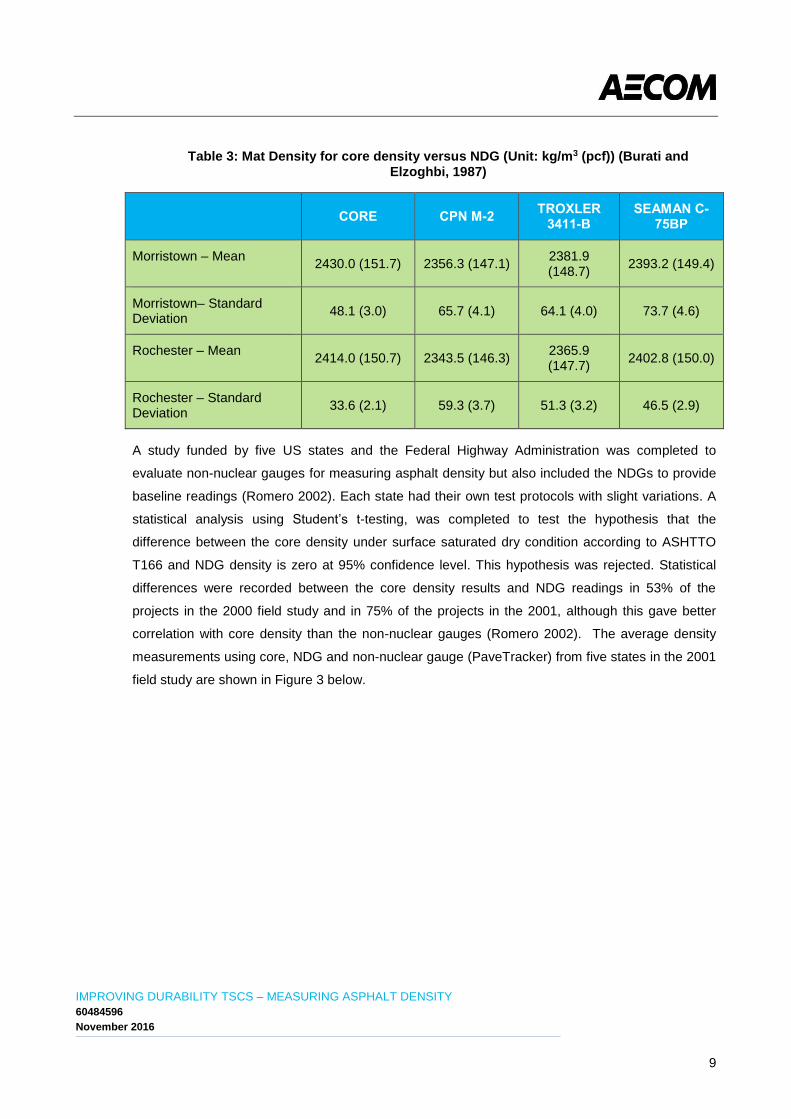
A study funded by five US states and the Federal Highway Administration was completed to
evaluate non-nuclear gauges for measuring asphalt density but also included the NDGs to provide
baseline readings (Romero 2002). Each state had their own test protocols with slight variations. A
statistical analysis using Student’s t-testing, was completed to test the hypothesis that the
difference between the core density under surface saturated dry condition according to ASHTTO
T166 and NDG density is zero at 95% confidence level. This hypothesis was rejected. Statistical
differences were recorded between the core density results and NDG readings in 53% of the
projects in the 2000 field study and in 75% of the projects in the 2001, although this gave better
correlation with core density than the non-nuclear gauges (Romero 2002). The average density
measurements using core, NDG and non-nuclear gauge (PaveTracker) from five states in the 2001
field study are shown in Figure 3 below.
IMPROVING DURABILITY TSCS – MEASURING ASPHALT DENSITY
60484596
November 2016
10
Figure 3 Average Density by Core, NDG & PaveTracker (Romero 2002)
Studies in six US States (California, Pennsylvania, Virginia, Nevada, Texas and Maine) concluded
that the NDG should only be used for quality control rather than for quality assurance. Conversely
in Connecticut, NDG was accepted for quality assurance and for payment certification. The
Connecticut Department of Transportation (Conn DoT) performed a study in 2003 and 2004 aiming
to develop a correlation between core density and NDG readings based on the data from seven
projects (Padlo et al 2005). The target compaction thickness was 2 inches (31.6 mm) in all
projects. The NDG results were found to be inconsistent from the six gauges used and also
inconsistent with the core density results. The discrepancies between the core densities (vacuum
sealed density in accordance with AASHTO TP 69) and the NDG measured densities varied from
0.3% to 1.2% of the maximum theoretical density (MTD), higher than 0.1% MTD, which was used
by Conn DoT for acceptance of projects for payment. Core densities measured by three individual
laboratories also had large variations. A linear regression analysis was performed to study the
effect of mat thickness on the discrepancies. The local mat thicknesses obtained by the core
depths ranged from 1.370 inches (21.6 mm) to 2.796 inches (44.1 mm). The linear regression
results are summarised in Table 4. The negative slope values indicate that as the thickness of
HMA mat increases the error in NDG density reduces. It was suspected that the NDG readings
were affected by the underlying pavement density on thinner pavements. The correlation
coefficient R2 is very low indicating poor linear correlation between the mat thickness and the NDG
errors. The effect of NDG orientation and pavement temperature on the density results was found
not to be influential. Multiple readings at each test location were recommended. A comparison
IMPROVING DURABILITY TSCS – MEASURING ASPHALT DENSITY
60484596
November 2016
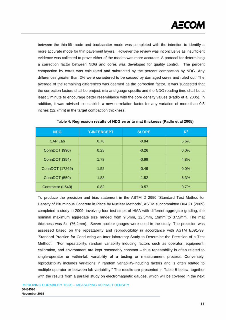
11
between the thin-lift mode and backscatter mode was completed with the intention to identify a
more accurate mode for thin pavement layers. However the review was inconclusive as insufficient
evidence was collected to prove either of the modes was more accurate. A protocol for determining
a correction factor between NDG and cores was developed for quality control. The percent
compaction by cores was calculated and subtracted by the percent compaction by NDG. Any
differences greater than 2% were considered to be caused by damaged cores and ruled out. The
average of the remaining differences was deemed as the correction factor. It was suggested that
the correction factors shall be project, mix and gauge specific and the NDG reading time shall be at
least 1 minute to encourage better resemblance with the core density values (Padlo et al 2005). In
addition, it was advised to establish a new correlation factor for any variation of more than 0.5
inches (12.7mm) in the target compaction thickness.
Table 4: Regression results of NDG error to mat thickness (Padlo et al 2005)
NDG Y-INTERCEPT SLOPE R2
CAP Lab 0.76 -0.94 5.6%
ConnDOT (990) 0.23 -0.26 0.0%
ConnDOT (354) 1.78 -0.99 4.8%
ConnDOT (17269) 1.52 -0.49 0.0%
ConnDOT (559) 1.83 -1.52 6.3%
Contractor (L540) 0.82 -0.57 0.7%
To produce the precision and bias statement in the ASTM D 2950 ‘Standard Test Method for
Density of Bituminous Concrete in Place by Nuclear Methods’, ASTM subcommittee D04.21 (2009)
completed a study in 2009, involving four test strips of HMA with different aggregate grading, the
nominal maximum aggregate size ranged from 9.5mm, 12.5mm, 19mm to 37.5mm. The mat
thickness was 3in (76.2mm). Seven nuclear gauges were used in the study. The precision was
assessed based on the repeatability and reproducibility in accordance with ASTM E691-99,
‘Standard Practice for Conducting an Inter-laboratory Study to Determine the Precision of a Test
Method’. “For repeatability, random variability inducing factors such as operator, equipment,
calibration, and environment are kept reasonably constant – thus repeatability is often related to
single-operator or within-lab variability of a testing or measurement process. Conversely,
reproducibility includes variations in random variability-inducing factors and is often related to
multiple operator or between-lab variability.” The results are presented in Table 5 below, together
with the results from a parallel study on electromagnetic gauges, which will be covered in the next
IMPROVING DURABILITY TSCS – MEASURING ASPHALT DENSITY
60484596
November 2016
12
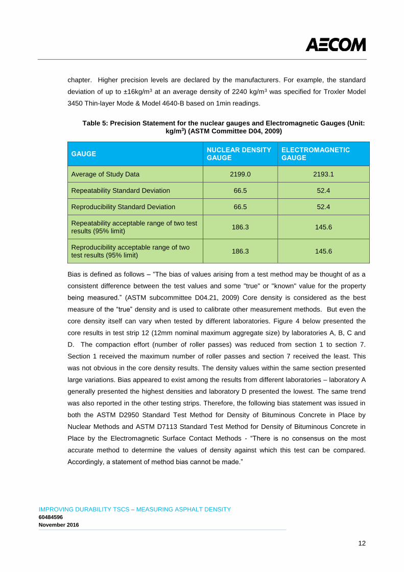
chapter. Higher precision levels are declared by the manufacturers. For example, the standard
deviation of up to ±16kg/m3 at an average density of 2240 kg/m3 was specified for Troxler Model
3450 Thin-layer Mode & Model 4640-B based on 1min readings.
Table 5: Precision Statement for the nuclear gauges and Electromagnetic Gauges (Unit: kg/m3) (ASTM Committee D04, 2009)
GAUGE NUCLEAR DENSITY GAUGE
ELECTROMAGNETIC GAUGE
Average of Study Data 2199.0 2193.1
Repeatability Standard Deviation 66.5 52.4
Reproducibility Standard Deviation 66.5 52.4
Repeatability acceptable range of two test results (95% limit)
186.3 145.6
Reproducibility acceptable range of two test results (95% limit)
186.3 145.6
Bias is defined as follows – “The bias of values arising from a test method may be thought of as a
consistent difference between the test values and some "true" or "known" value for the property
being measured.” (ASTM subcommittee D04.21, 2009) Core density is considered as the best
measure of the “true” density and is used to calibrate other measurement methods. But even the
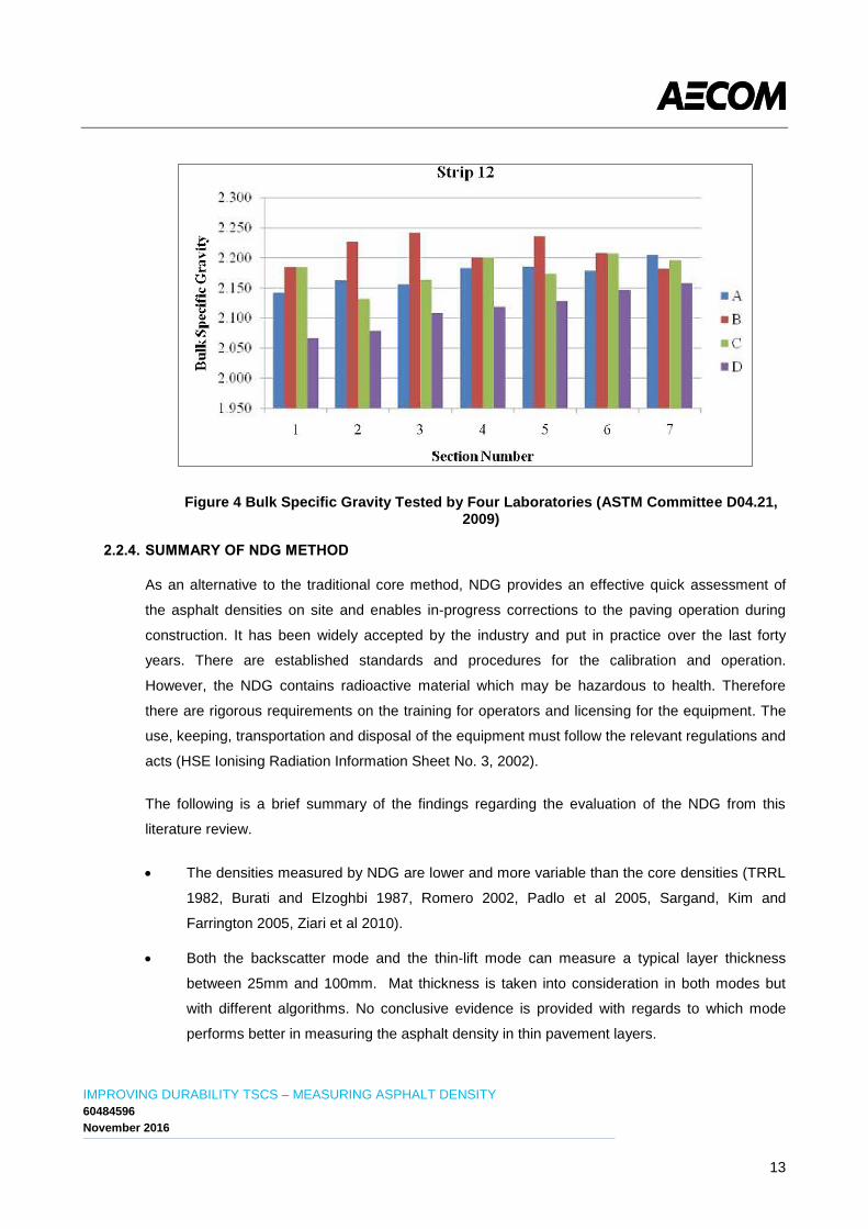
core density itself can vary when tested by different laboratories. Figure 4 below presented the
core results in test strip 12 (12mm nominal maximum aggregate size) by laboratories A, B, C and
D. The compaction effort (number of roller passes) was reduced from section 1 to section 7.
Section 1 received the maximum number of roller passes and section 7 received the least. This
was not obvious in the core density results. The density values within the same section presented
large variations. Bias appeared to exist among the results from different laboratories – laboratory A
generally presented the highest densities and laboratory D presented the lowest. The same trend
was also reported in the other testing strips. Therefore, the following bias statement was issued in
both the ASTM D2950 Standard Test Method for Density of Bituminous Concrete in Place by
Nuclear Methods and ASTM D7113 Standard Test Method for Density of Bituminous Concrete in
Place by the Electromagnetic Surface Contact Methods - “There is no consensus on the most
accurate method to determine the values of density against which this test can be compared.
Accordingly, a statement of method bias cannot be made.”
IMPROVING DURABILITY TSCS – MEASURING ASPHALT DENSITY
60484596
November 2016
13
Figure 4 Bulk Specific Gravity Tested by Four Laboratories (ASTM Committee D04.21, 2009)
2.2.4. SUMMARY OF NDG METHOD
As an alternative to the traditional core method, NDG provides an effective quick assessment of
the asphalt densities on site and enables in-progress corrections to the paving operation during
construction. It has been widely accepted by the industry and put in practice over the last forty
years. There are established standards and procedures for the calibration and operation.
However, the NDG contains radioactive material which may be hazardous to health. Therefore
there are rigorous requirements on the training for operators and licensing for the equipment. The
use, keeping, transportation and disposal of the equipment must follow the relevant regulations and
acts (HSE Ionising Radiation Information Sheet No. 3, 2002).
The following is a brief summary of the findings regarding the evaluation of the NDG from this
literature review.
The densities measured by NDG are lower and more variable than the core densities (TRRL
1982, Burati and Elzoghbi 1987, Romero 2002, Padlo et al 2005, Sargand, Kim and
Farrington 2005, Ziari et al 2010).
Both the backscatter mode and the thin-lift mode can measure a typical layer thickness
between 25mm and 100mm. Mat thickness is taken into consideration in both modes but
with different algorithms. No conclusive evidence is provided with regards to which mode
performs better in measuring the asphalt density in thin pavement layers.
IMPROVING DURABILITY TSCS – MEASURING ASPHALT DENSITY
60484596
November 2016
14
The density measured by the back-scatter mode and thin-lift mode was reported to be more
influenced by the material at the top 50mm in thick pavement layers, whilst the density of
thin pavement layers was reported to be affected by the substrate material. ASTM D2950
suggests “For lift thicknesses of 51 mm [2 in.] or less, the backscatter mode is suggested; for
lift thicknesses greater than 51 mm [2 in.] the direct transmission mode is suggested. Thin lift
gauges can be used for lift thicknesses up to 102 mm [4 in.]”.
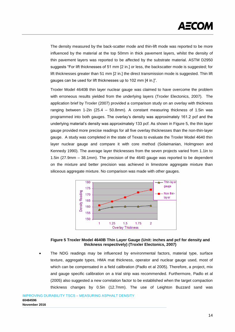
Troxler Model 4640B thin layer nuclear gauge was claimed to have overcome the problem
with erroneous results yielded from the underlying layers (Troxler Electonics, 2007). The
application brief by Troxler (2007) provided a comparison study on an overlay with thickness
ranging between 1-2in (25.4 – 50.8mm). A constant measuring thickness of 1.5in was
programmed into both gauges. The overlay’s density was approximately 161.2 pcf and the
underlying material’s density was approximately 133 pcf. As shown in Figure 5, the thin layer
gauge provided more precise readings for all five overlay thicknesses than the non-thin-layer
gauge. A study was completed in the state of Texas to evaluate the Troxler Model 4640 thin
layer nuclear gauge and compare it with core method (Solaimanian, Holmgreen and
Kennedy 1990). The average layer thicknesses from the seven projects varied from 1.1in to
1.5in (27.9mm – 38.1mm). The precision of the 4640 gauge was reported to be dependent
on the mixture and better precision was achieved in limestone aggregate mixture than
siliceous aggregate mixture. No comparison was made with other gauges.
Figure 5 Troxler Model 4640B Thin Layer Gauge (Unit: inches and pcf for density and thickness respectively) (Troxler Electonics, 2007)
The NDG readings may be influenced by environmental factors, material type, surface
texture, aggregate types, HMA mat thickness, operator and nuclear gauge used, most of
which can be compensated in a field calibration (Padlo et al 2005). Therefore, a project, mix
and gauge specific calibration on a trial strip was recommended. Furthermore, Padlo et al
(2005) also suggested a new correlation factor to be established when the target compaction
thickness changes by 0.5in (12.7mm). The use of Leighton Buzzard sand was
IMPROVING DURABILITY TSCS – MEASURING ASPHALT DENSITY
60484596
November 2016
15
recommended in TRL report 754 to fill the surface texture and ensure a firm contact between
the gauge and the surface of the paving material for each measurement. ASTM D2950 also
stressed the maximum contact is critical and shall be achieve by filling the voids by fine
sand.
No significant influence by temperature and moisture was reported for NDG measurement. It
must be noted however, ASTM D2590 warns “Do not leave the gauge on a hot surface for
an extended period of time. Prolonged high temperatures may adversely affect the
instrument’s electronics. The gauge should be allowed to cool between measurements”.
The precision level was assessed in a field study according to the repeatability and
reproducibility in accordance with ASTM E691-99. Both the single-operator precision and
multi-laboratory precision are stated in ASTM D2950.
3. DENSITY MEASUREMENT– OTHER METHODS
In addition to the above methods, BS 594987: 2015 Clause 9.4.2 and UK Manual of Contract
Documents for Highway Works (MCHW) Volume 2 Notes for Guidance on the Specification for
Highway Works Clause NG929 (08/08) also permit the use of alternative indirect density measuring
devices other than nuclear density gauges. The calibration and operation protocol is provided in
BS 594987 Annex I for all indirect density gauges including NDGs. The following chapter will
introduce other technologies, beginning with capacitive electromagnetic method, which is receiving
more industry recognition. Other technologies are also available, such as ground-penetrating radar,
step-frequency radar, ultrasound technology and automated field density prediction. However,
most of these are still at the research stage.
3.1. CAPACITIVE ELECTROMAGNETIC METHOD – PQI & PAVETRACKER
3.1.1. HISTORY
The first non-nuclear density gauge used to measure HMA density was made available by
TransTech Systems Inc. in 1998. The very first model, called Pavement Quality Indicator (PQI),
later referred to as “PQI-100”, was reported to have “serious problems when the moisture is
present in the mixture”. To address the problem, the moisture level is measured and recorded in
the later model, PQI-300, through the lag or phase angle in the electrical signal. This value is
displayed as “H2O” reading on the PQI interface and contributes to the built-in corrective algorithm
to compensate for the moisture effect. Conflicting views were taken by different authors on its
performance (Romero 2000, Henault 2001, Romero 2002). TransTech made further improvements
on the PQI models – PQI 302 were available in 2005 and PQI 303 in 2007. The latest model, PQI
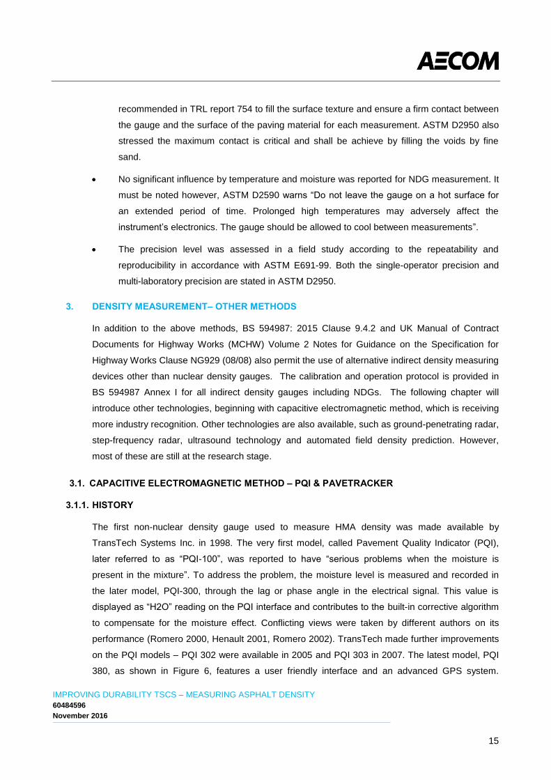
380, as shown in Figure 6, features a user friendly interface and an advanced GPS system.
IMPROVING DURABILITY TSCS – MEASURING ASPHALT DENSITY
60484596
November 2016
16
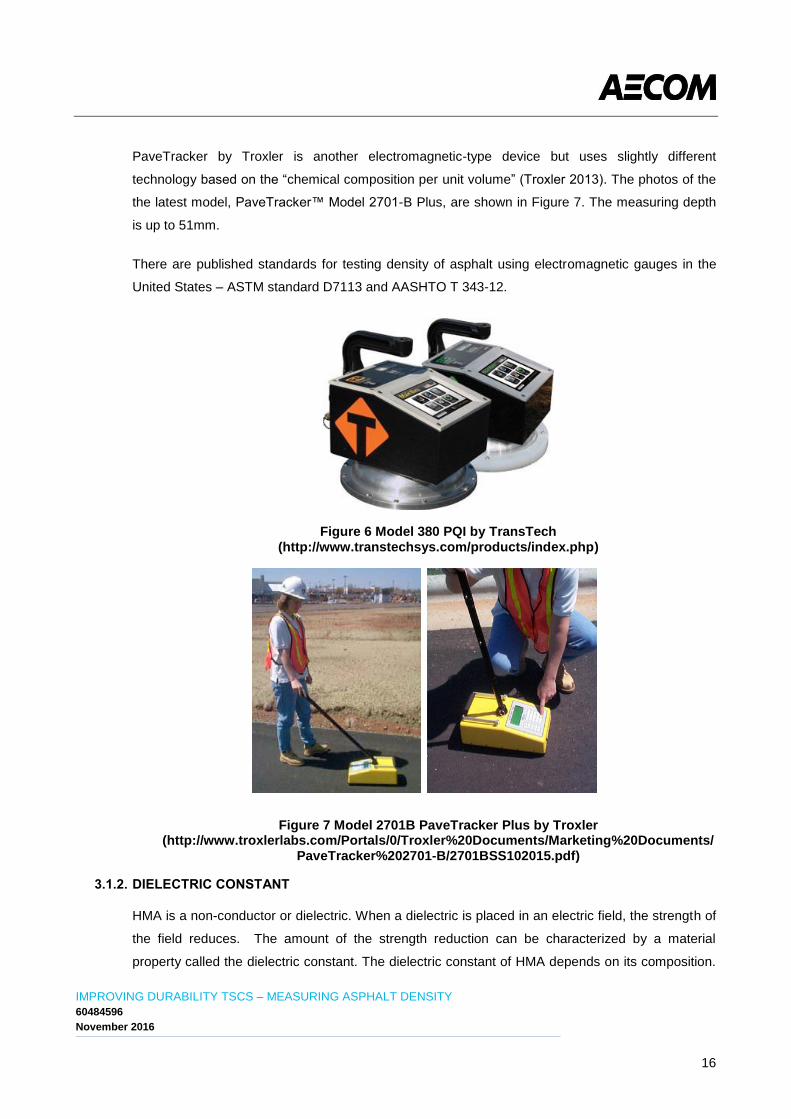
PaveTracker by Troxler is another electromagnetic-type device but uses slightly different
technology based on the “chemical composition per unit volume” (Troxler 2013). The photos of the
the latest model, PaveTracker™ Model 2701-B Plus, are shown in Figure 7. The measuring depth
is up to 51mm.
There are published standards for testing density of asphalt using electromagnetic gauges in the
United States – ASTM standard D7113 and AASHTO T 343-12.
Figure 6 Model 380 PQI by TransTech (http://www.transtechsys.com/products/index.php)
Figure 7 Model 2701B PaveTracker Plus by Troxler (http://www.troxlerlabs.com/Portals/0/Troxler%20Documents/Marketing%20Documents/
PaveTracker%202701-B/2701BSS102015.pdf)
3.1.2. DIELECTRIC CONSTANT
HMA is a non-conductor or dielectric. When a dielectric is placed in an electric field, the strength of
the field reduces. The amount of the strength reduction can be characterized by a material
property called the dielectric constant. The dielectric constant of HMA depends on its composition.
IMPROVING DURABILITY TSCS – MEASURING ASPHALT DENSITY
60484596
November 2016
17
A homogeneous HMA typically ranges from 2.5 to 3.2. The dielectric constant for water ranges
from 4 to 88 (Mason 2008). The PQI and PaveTracker operate in the same principle by assessing
the change in an electric field to determine the dielectric constant of the tested material. Then the
density can be calculated by comparing the dielectric constants with a material with a known
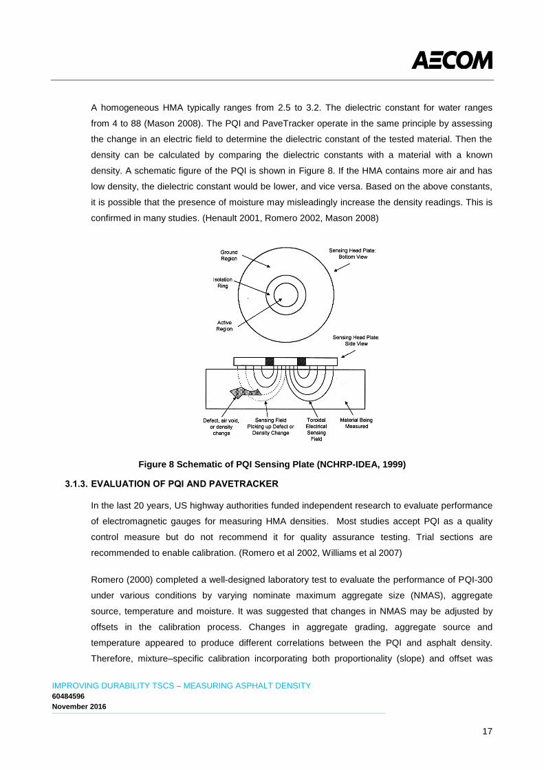
density. A schematic figure of the PQI is shown in Figure 8. If the HMA contains more air and has
low density, the dielectric constant would be lower, and vice versa. Based on the above constants,
it is possible that the presence of moisture may misleadingly increase the density readings. This is
confirmed in many studies. (Henault 2001, Romero 2002, Mason 2008)
Figure 8 Schematic of PQI Sensing Plate (NCHRP-IDEA, 1999)
3.1.3. EVALUATION OF PQI AND PAVETRACKER
In the last 20 years, US highway authorities funded independent research to evaluate performance
of electromagnetic gauges for measuring HMA densities. Most studies accept PQI as a quality
control measure but do not recommend it for quality assurance testing. Trial sections are
recommended to enable calibration. (Romero et al 2002, Williams et al 2007)
Romero (2000) completed a well-designed laboratory test to evaluate the performance of PQI-300
under various conditions by varying nominate maximum aggregate size (NMAS), aggregate
source, temperature and moisture. It was suggested that changes in NMAS may be adjusted by
offsets in the calibration process. Changes in aggregate grading, aggregate source and
temperature appeared to produce different correlations between the PQI and asphalt density.
Therefore, mixture–specific calibration incorporating both proportionality (slope) and offset was
IMPROVING DURABILITY TSCS – MEASURING ASPHALT DENSITY
60484596
November 2016
18
recommended. The PQI manual (2003) details the procedure for both offset and slope calibrations.
However, the slope calibration was highlighted for factory use only. The experiment used H2O
display on the PQI devices to monitor moisture changes and came to a conclusion that as long as
the moisture is kept constant and relatively low (below 5% H2O number in the experiment), PQI-
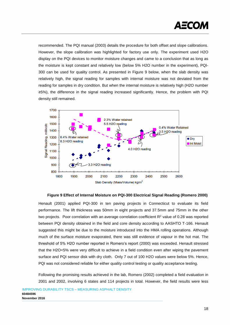
300 can be used for quality control. As presented in Figure 9 below, when the slab density was
relatively high, the signal reading for samples with internal moisture was not deviated from the
reading for samples in dry condition. But when the internal moisture is relatively high (H2O number
≥5%), the difference in the signal reading increased significantly. Hence, the problem with PQI
density still remained.
Figure 9 Effect of Internal Moisture on PQI-300 Electrical Signal Reading (Romero 2000)
Henault (2001) applied PQI-300 in ten paving projects in Connecticut to evaluate its field
performance. The lift thickness was 50mm in eight projects and 37.5mm and 75mm in the other
two projects. Poor correlation with an average correlation coefficient R2 value of 0.28 was reported
between PQI density obtained in the field and core density according to AASHTO T-166. Henault
suggested this might be due to the moisture introduced into the HMA rolling operations. Although
much of the surface moisture evaporated, there was still evidence of vapour in the hot mat. The
threshold of 5% H2O number reported in Romero’s report (2000) was exceeded. Henault stressed
that the H2O<5% were very difficult to achieve in a field condition even after wiping the pavement
surface and PQI sensor disk with dry cloth. Only 7 out of 100 H2O values were below 5%. Hence,
PQI was not considered reliable for either quality control testing or quality acceptance testing.
Following the promising results achieved in the lab, Romero (2002) completed a field evaluation in
2001 and 2002, involving 6 states and 114 projects in total. However, the field results were less
IMPROVING DURABILITY TSCS – MEASURING ASPHALT DENSITY
60484596
November 2016
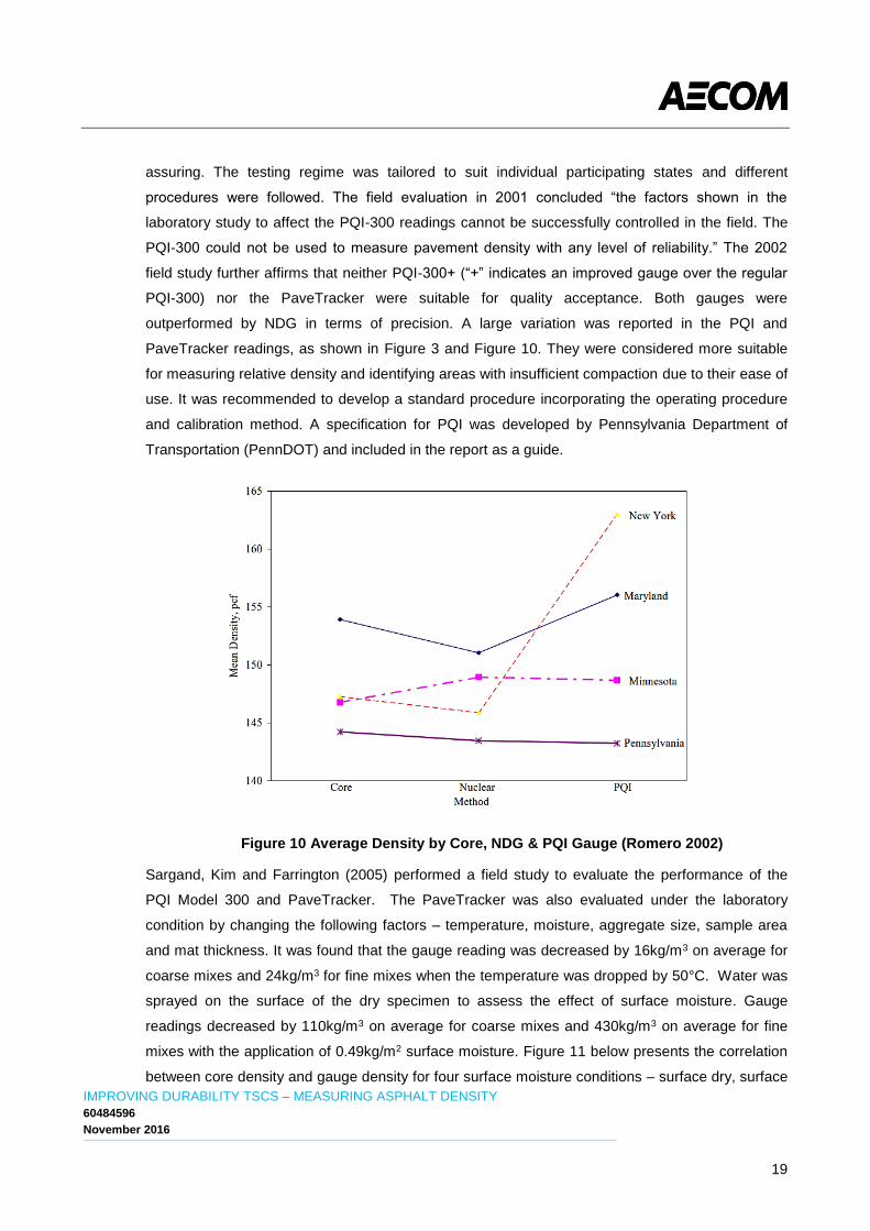
19
assuring. The testing regime was tailored to suit individual participating states and different
procedures were followed. The field evaluation in 2001 concluded “the factors shown in the
laboratory study to affect the PQI-300 readings cannot be successfully controlled in the field. The
PQI-300 could not be used to measure pavement density with any level of reliability.” The 2002
field study further affirms that neither PQI-300+ (“+” indicates an improved gauge over the regular
PQI-300) nor the PaveTracker were suitable for quality acceptance. Both gauges were
outperformed by NDG in terms of precision. A large variation was reported in the PQI and
PaveTracker readings, as shown in Figure 3 and Figure 10. They were considered more suitable
for measuring relative density and identifying areas with insufficient compaction due to their ease of
use. It was recommended to develop a standard procedure incorporating the operating procedure
and calibration method. A specification for PQI was developed by Pennsylvania Department of
Transportation (PennDOT) and included in the report as a guide.
Figure 10 Average Density by Core, NDG & PQI Gauge (Romero 2002)
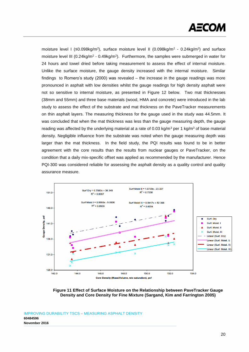
Sargand, Kim and Farrington (2005) performed a field study to evaluate the performance of the
PQI Model 300 and PaveTracker. The PaveTracker was also evaluated under the laboratory
condition by changing the following factors – temperature, moisture, aggregate size, sample area
and mat thickness. It was found that the gauge reading was decreased by 16kg/m3 on average for
coarse mixes and 24kg/m3 for fine mixes when the temperature was dropped by 50°C. Water was
sprayed on the surface of the dry specimen to assess the effect of surface moisture. Gauge
readings decreased by 110kg/m3 on average for coarse mixes and 430kg/m3 on average for fine
mixes with the application of 0.49kg/m2 surface moisture. Figure 11 below presents the correlation
between core density and gauge density for four surface moisture conditions – surface dry, surface
IMPROVING DURABILITY TSCS – MEASURING ASPHALT DENSITY
60484596
November 2016
20
moisture level I (≤0.098kg/m2), surface moisture level II (0.098kg/m2 - 0.24kg/m2) and surface
moisture level III (0.24kg/m2 - 0.49kg/m2). Furthermore, the samples were submerged in water for
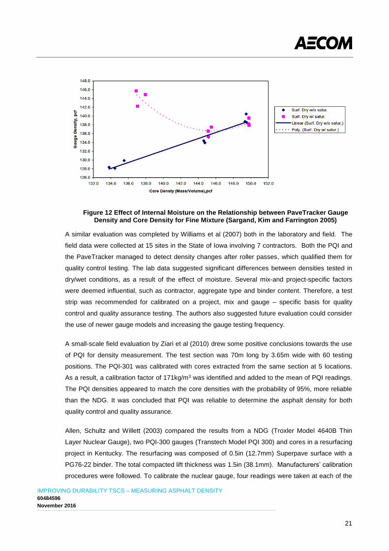
24 hours and towel dried before taking measurement to assess the effect of internal moisture.
Unlike the surface moisture, the gauge density increased with the internal moisture. Similar
findings to Romero’s study (2000) was revealed – the increase in the gauge readings was more
pronounced in asphalt with low densities whilst the gauge readings for high density asphalt were
not so sensitive to internal moisture, as presented in Figure 12 below. Two mat thicknesses
(38mm and 55mm) and three base materials (wood, HMA and concrete) were introduced in the lab
study to assess the effect of the substrate and mat thickness on the PaveTracker measurements
on thin asphalt layers. The measuring thickness for the gauge used in the study was 44.5mm. It
was concluded that when the mat thickness was less than the gauge measuring depth, the gauge
reading was affected by the underlying material at a rate of 0.03 kg/m3 per 1 kg/m3 of base material
density. Negligible influence from the substrate was noted when the gauge measuring depth was
larger than the mat thickness. In the field study, the PQI results was found to be in better
agreement with the core results than the results from nuclear gauges or PaveTracker, on the
condition that a daily mix-specific offset was applied as recommended by the manufacturer. Hence
PQI-300 was considered reliable for assessing the asphalt density as a quality control and quality
assurance measure.
Figure 11 Effect of Surface Moisture on the Relationship between PaveTracker Gauge Density and Core Density for Fine Mixture (Sargand, Kim and Farrington 2005)
IMPROVING DURABILITY TSCS – MEASURING ASPHALT DENSITY
60484596
November 2016
21
Figure 12 Effect of Internal Moisture on the Relationship between PaveTracker Gauge Density and Core Density for Fine Mixture (Sargand, Kim and Farrington 2005)
A similar evaluation was completed by Williams et al (2007) both in the laboratory and field. The
field data were collected at 15 sites in the State of Iowa involving 7 contractors. Both the PQI and
the PaveTracker managed to detect density changes after roller passes, which qualified them for
quality control testing. The lab data suggested significant differences between densities tested in
dry/wet conditions, as a result of the effect of moisture. Several mix-and project-specific factors
were deemed influential, such as contractor, aggregate type and binder content. Therefore, a test
strip was recommended for calibrated on a project, mix and gauge – specific basis for quality
control and quality assurance testing. The authors also suggested future evaluation could consider
the use of newer gauge models and increasing the gauge testing frequency.
A small-scale field evaluation by Ziari et al (2010) drew some positive conclusions towards the use
of PQI for density measurement. The test section was 70m long by 3.65m wide with 60 testing
positions. The PQI-301 was calibrated with cores extracted from the same section at 5 locations.
As a result, a calibration factor of 171kg/m3 was identified and added to the mean of PQI readings.
The PQI densities appeared to match the core densities with the probability of 95%, more reliable
than the NDG. It was concluded that PQI was reliable to determine the asphalt density for both
quality control and quality assurance.
Allen, Schultz and Willett (2003) compared the results from a NDG (Troxler Model 4640B Thin
Layer Nuclear Gauge), two PQI-300 gauges (Transtech Model PQI 300) and cores in a resurfacing
project in Kentucky. The resurfacing was composed of 0.5in (12.7mm) Superpave surface with a
PG76-22 binder. The total compacted lift thickness was 1.5in (38.1mm). Manufacturers’ calibration
procedures were followed. To calibrate the nuclear gauge, four readings were taken at each of the
IMPROVING DURABILITY TSCS – MEASURING ASPHALT DENSITY
60484596
November 2016
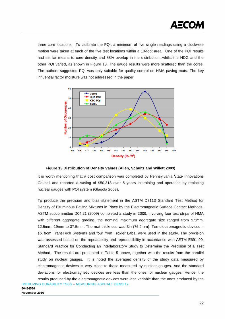
22
three core locations. To calibrate the PQI, a minimum of five single readings using a clockwise
motion were taken at each of the five test locations within a 10-foot area. One of the PQI results
had similar means to core density and 88% overlap in the distribution, whilst the NDG and the
other PQI varied, as shown in Figure 13. The gauge results were more scattered than the cores.
The authors suggested PQI was only suitable for quality control on HMA paving mats. The key
influential factor moisture was not addressed in the paper.
Figure 13 Distribution of Density Values (Allen, Schultz and Willett 2003)
It is worth mentioning that a cost comparison was completed by Pennsylvania State Innovations
Council and reported a saving of $50,318 over 5 years in training and operation by replacing
nuclear gauges with PQI system (Glagola 2003).
To produce the precision and bias statement in the ASTM D7113 Standard Test Method for
Density of Bituminous Paving Mixtures in Place by the Electromagnetic Surface Contact Methods,
ASTM subcommittee D04.21 (2009) completed a study in 2009, involving four test strips of HMA
with different aggregate grading, the nominal maximum aggregate size ranged from 9.5mm,
12.5mm, 19mm to 37.5mm. The mat thickness was 3in (76.2mm). Ten electromagnetic devices –
six from TransTech Systems and four from Troxler Labs, were used in the study. The precision
was assessed based on the repeatability and reproducibility in accordance with ASTM E691-99,
Standard Practice for Conducting an Interlaboratory Study to Determine the Precision of a Test
Method. The results are presented in Table 5 above, together with the results from the parallel
study on nuclear gauges. It is noted the averaged density of the study data measured by
electromagnetic devices is very close to those measured by nuclear gauges. And the standard
deviations for electromagnetic devices are less than the ones for nuclear gauges. Hence, the
results produced by the electromagnetic devices were less variable than the ones produced by the
IMPROVING DURABILITY TSCS – MEASURING ASPHALT DENSITY
60484596
November 2016
23
NDG. As explained in Section 2.2.3, no bias statement was issued as no “true” or “known” value of
pavement density is available. Higher precision levels are declared by the manufacturers. For
example, the standard deviation of up to ±3.2kg/m3 was specified for PaveTracker™ Model 2701-B
Plus.
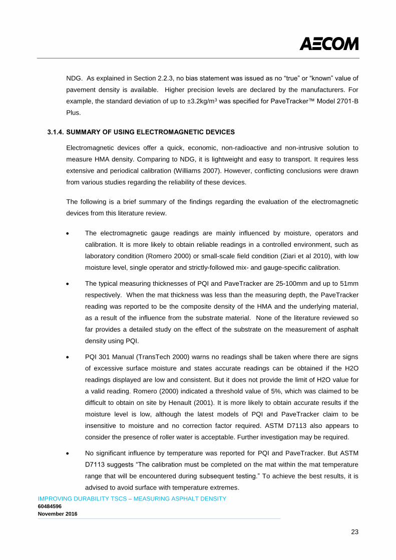
3.1.4. SUMMARY OF USING ELECTROMAGNETIC DEVICES
Electromagnetic devices offer a quick, economic, non-radioactive and non-intrusive solution to
measure HMA density. Comparing to NDG, it is lightweight and easy to transport. It requires less
extensive and periodical calibration (Williams 2007). However, conflicting conclusions were drawn
from various studies regarding the reliability of these devices.
The following is a brief summary of the findings regarding the evaluation of the electromagnetic
devices from this literature review.
The electromagnetic gauge readings are mainly influenced by moisture, operators and
calibration. It is more likely to obtain reliable readings in a controlled environment, such as
laboratory condition (Romero 2000) or small-scale field condition (Ziari et al 2010), with low
moisture level, single operator and strictly-followed mix- and gauge-specific calibration.
The typical measuring thicknesses of PQI and PaveTracker are 25-100mm and up to 51mm
respectively. When the mat thickness was less than the measuring depth, the PaveTracker
reading was reported to be the composite density of the HMA and the underlying material,
as a result of the influence from the substrate material. None of the literature reviewed so
far provides a detailed study on the effect of the substrate on the measurement of asphalt
density using PQI.
PQI 301 Manual (TransTech 2000) warns no readings shall be taken where there are signs
of excessive surface moisture and states accurate readings can be obtained if the H2O
readings displayed are low and consistent. But it does not provide the limit of H2O value for
a valid reading. Romero (2000) indicated a threshold value of 5%, which was claimed to be
difficult to obtain on site by Henault (2001). It is more likely to obtain accurate results if the
moisture level is low, although the latest models of PQI and PaveTracker claim to be
insensitive to moisture and no correction factor required. ASTM D7113 also appears to
consider the presence of roller water is acceptable. Further investigation may be required.
No significant influence by temperature was reported for PQI and PaveTracker. But ASTM
D7113 suggests “The calibration must be completed on the mat within the mat temperature
range that will be encountered during subsequent testing.” To achieve the best results, it is
advised to avoid surface with temperature extremes.
IMPROVING DURABILITY TSCS – MEASURING ASPHALT DENSITY
60484596
November 2016
24
A mixture specific calibration incorporating both offset and slope was recommended
(Williams et al 2007). The offset calibration shall be completed on site by operators. The
procedure provided in ASTM D7113 may be used jointly with manufacturers’ guidance. The
slope calibration shall be completed by manufacturers at least once a year.
The precision level was assessed in a field study according to the repeatability and
reproducibility in accordance with ASTM E691-99. Both the single-operator precision and
multi-laboratory precision are stated in ASTM D7113.
The effect of magnetic fields on the electromagnetic gauges is unclear. Therefore it might be
reasonable to avoid using the devices near power lines.
The gauges used in most of the literature are the early models. Improvements have been
made to the devices over the years. Further evaluation using the newer models may be
required to verify the current conclusions drawn based on the old models.
3.2. ELECTROMAGNETIC WAVE-BASED METHOD – RADAR SYSTEMS
Ground-Penetrating Radar (GPR) has been used in pavement engineering to measure layer
thicknesses and detect pavement distresses since 1970s. It was first considered as an approach to
measure asphalt density and void content by Al-Qadi (1992), which was followed by the
development of a computer program to predict asphalt densities and water contents (Lytton 1995).
Building on these, more studies were completed in recent years. But until now, it is still at the
research stage and not ready for the industry yet.
The GPR method is electromagnetic-wave-based. Short electromagnetic pulses are emitted from
an antenna and penetrating through the pavement. Echoes created at pavement surface and
internal inhomogeneity are reflected back and captured by a data acquisition system. The dielectric
constant can be estimated based on the amplitude and phase of the reflected signals. Once the
correlation between the dielectric constant of an asphalt mixture and its density is determined, the
asphalt density can be predicted through a GPR survey. There are two established correlations
based on electromagnetic mixing theory – Complex Refractive Index Model (CRIM) and modified
Bottcher model, as demonstrated in Eq. 1 and 2 respectively. The latter assumed the air particles
and aggregates in the mixture were in spherical shape.
Al-Qadi et al (2011) further improved the modified Bottcher model by the introduction of a shape
factor, u, to account for non-spherical inclusions and established the Al-Qadi Lahouar Leng (ALL)
Model, shown in Eq. 3. This was validated using in-service pavement data. The pavement
structure is composed of 50mm thick new asphalt overlay with five different mixtures over an old
asphalt overlay and concrete pavement. Steel slags were introduced in two of the mixes: The
IMPROVING DURABILITY TSCS – MEASURING ASPHALT DENSITY
60484596
November 2016
25
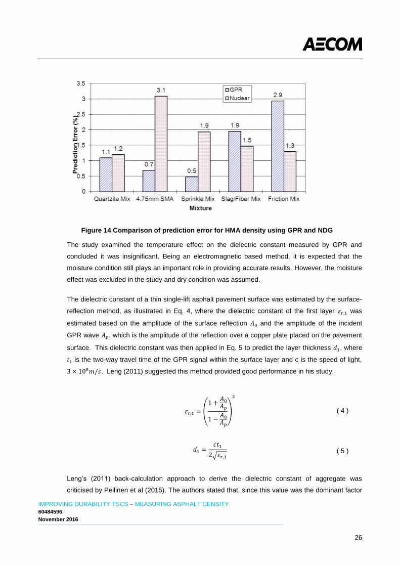
fibre/slag mix contained 20% slags and the friction mix contained 36% slags. Both the GPR results
and the nuclear density gauge results were compared with the core densities under surface
saturated dry condition. A better precision of in situ density using GPR was achieved than that
using NDG in the mixes without slags, as shown in Figure 14. The average prediction errors varied
from 0.5% to 1.1%. In the mixes with steel slags, the average prediction errors of GPR results
were 1.9% and 2.9%, higher than the results using NDG. It was suspected that the high dielectric
constant of metal and its random distribution in the mixes might have contributed to the errors. Two
calibration cores were recommended to produce a reliable εb.
𝐺𝑚𝑏 =
√𝜀𝐴𝐶 − 1
𝑃𝑏
𝐺𝑏√𝜀𝑏 +
(1 − 𝑃𝑏)𝐺𝑠𝑒
√𝜀𝑠 −1
𝐺𝑚𝑚
( 1 )
𝐺𝑚𝑏 =
𝜀𝐴𝐶 − 𝜀𝑏
3𝜀𝐴𝐶−
1 − 𝜀𝑏
1 + 2𝜀𝐴𝐶
(𝜀𝑠 − 𝜀𝑏
𝜀𝑠 + 2𝜀𝐴𝐶) (
1 − 𝑃𝑏
𝐺𝑠𝑒) − (
1 − 𝜀𝑏
1 + 2𝜀𝐴𝐶) (
1𝐺𝑚𝑚
) ( 2 )
𝐺𝑚𝑏 =
𝜀𝐴𝐶 − 𝜀𝑏
3𝜀𝐴𝐶 − (𝑢 − 2)𝜀𝑏−
1 − 𝜀𝑏
1 − (𝑢 − 2)𝜀𝑏 + 2𝜀𝐴𝐶
(𝜀𝑠 − 𝜀𝑏
𝜀𝑠 − (𝑢 − 2)𝜀𝑏 + 2𝜀𝐴𝐶) (
1 − 𝑃𝑏
𝐺𝑠𝑒) − (
1 − 𝜀𝑏
1 − (𝑢 − 2)𝜀𝑏 + 2𝜀𝐴𝐶) (
1𝐺𝑚𝑚
) ( 3 )
Where: Gmb – bulk specific gravity of asphalt mixture;
Gmm – maximum specific gravity of asphalt mixture;
Gb – specific gravity of binder;
Gse – effective specific gravity of aggregate;
Gsb – bulk specific gravity of aggregate;
Pb – binder content;
εb – dielectric constant of binder;
εAC – dielectric constant of asphalt mixture;
εs – dielectric constant of aggregate
u – shape factor
IMPROVING DURABILITY TSCS – MEASURING ASPHALT DENSITY
60484596
November 2016
26
Figure 14 Comparison of prediction error for HMA density using GPR and NDG
The study examined the temperature effect on the dielectric constant measured by GPR and
concluded it was insignificant. Being an electromagnetic based method, it is expected that the
moisture condition still plays an important role in providing accurate results. However, the moisture
effect was excluded in the study and dry condition was assumed.
The dielectric constant of a thin single-lift asphalt pavement surface was estimated by the surface-
reflection method, as illustrated in Eq. 4, where the dielectric constant of the first layer 𝜀𝑟,1 was
estimated based on the amplitude of the surface reflection 𝐴0 and the amplitude of the incident
GPR wave 𝐴𝑝, which is the amplitude of the reflection over a copper plate placed on the pavement
surface. This dielectric constant was then applied in Eq. 5 to predict the layer thickness 𝑑1, where
𝑡1 is the two-way travel time of the GPR signal within the surface layer and c is the speed of light,
3 × 10⁸𝑚/𝑠. Leng (2011) suggested this method provided good performance in his study.
𝜀𝑟,1 = (
1 +𝐴0
𝐴𝑝
1 −𝐴0
𝐴𝑝
)
2
( 4 )
𝑑1 =
𝑐𝑡1
2√𝜀𝑟,1
( 5 )
Leng’s (2011) back-calculation approach to derive the dielectric constant of aggregate was
criticised by Pellinen et al (2015). The authors stated that, since this value was the dominant factor
IMPROVING DURABILITY TSCS – MEASURING ASPHALT DENSITY
60484596
November 2016
27
for dielectric value of asphalt mixture and it varied for different aggregates, this back-calculation
approach “may lead to large errors in assessing pavement density”. Fauchard et al (2013)
measured the dielectric constant of aggregate using cylindrical resonant cavities and reported a
variation from 4.5 to 7.7 for the tested samples of sandstones, quartzite, granite, limestone and
basalt etc. Not only the aggregate types but also same aggregate from different quarries appears
to have large variations in their dielectric constants. Pellinen et al (2015) further questioned the
calibration of GPR based on one core only whilst the antenna covered a larger footprint of 300mm
by 300mm (referred to as “volume element”). Attempts were made to quantify this variability by
introducing a representative volume element (RVE). It was reported that the bulk property void
content measured by GPR technique cannot be reliably calibrated using one core only and a
sensible RVE was still to be determined.
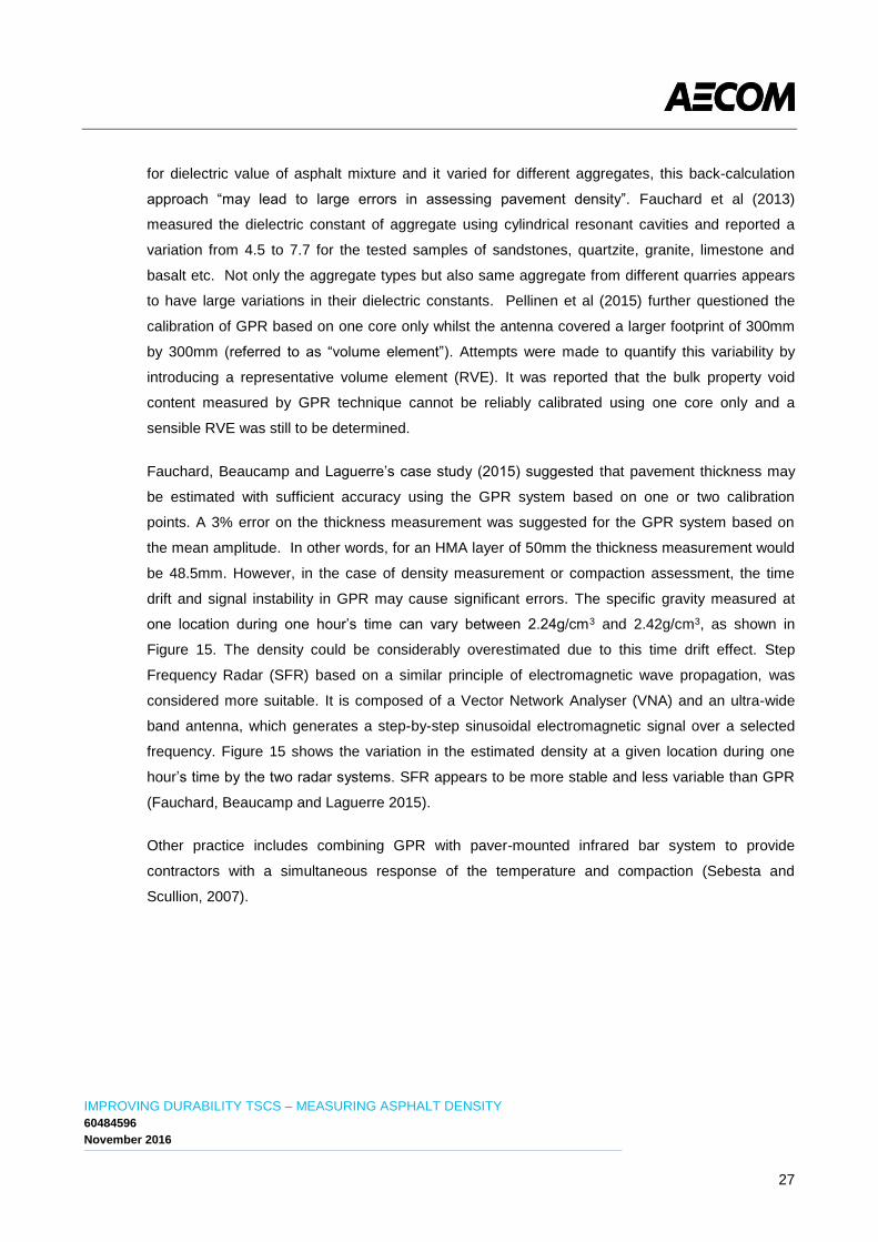
Fauchard, Beaucamp and Laguerre’s case study (2015) suggested that pavement thickness may
be estimated with sufficient accuracy using the GPR system based on one or two calibration
points. A 3% error on the thickness measurement was suggested for the GPR system based on
the mean amplitude. In other words, for an HMA layer of 50mm the thickness measurement would
be 48.5mm. However, in the case of density measurement or compaction assessment, the time
drift and signal instability in GPR may cause significant errors. The specific gravity measured at
one location during one hour’s time can vary between 2.24g/cm3 and 2.42g/cm3, as shown in
Figure 15. The density could be considerably overestimated due to this time drift effect. Step
Frequency Radar (SFR) based on a similar principle of electromagnetic wave propagation, was
considered more suitable. It is composed of a Vector Network Analyser (VNA) and an ultra-wide
band antenna, which generates a step-by-step sinusoidal electromagnetic signal over a selected
frequency. Figure 15 shows the variation in the estimated density at a given location during one
hour’s time by the two radar systems. SFR appears to be more stable and less variable than GPR
(Fauchard, Beaucamp and Laguerre 2015).
Other practice includes combining GPR with paver-mounted infrared bar system to provide
contractors with a simultaneous response of the temperature and compaction (Sebesta and
Scullion, 2007).
IMPROVING DURABILITY TSCS – MEASURING ASPHALT DENSITY
60484596
November 2016
28
Figure 15 Density by GPR & SFR (Fauchard, Beaucamp and Laguerre 2015)
Overall, the radar systems have the advantage of providing full coverage of the area with
continuous, efficient and non-intrusive density measurement. However, there are some obstacles
to overcome before this may be adopted by the industry in field density measurement.
Moisture is a major cause of inaccurate density assessment with all the electromagnetic-
based technologies. The presence of water in the pavement has a strong influence on the
dielectric constant measurements, and hence the density. The precision of the radar
systems in evaluating asphalt density is subjective to testing under dry condition, which is a
major limitation of this method. Al-Qadi et al (2011) also suggested a feasibility study to
predict the asphalt density and moisture content simultaneously using the GPR system.
The dielectric constant of aggregate has an influential role in the evaluation of asphalt
density using radars. Depending on the aggregates’ mineral composition, porosity, moisture
content and frequency, a variation of 4.5 – 7.7 was reported (Fauchard et al 2013). With the
increasing use of recycled aggregate in road construction, a practical and reliable procedure
for evaluating the aggregate dielectric constant is required to encourage accurate prediction
of asphalt density.
The dielectric constant of a thin single-lift layer was obtained by the amplitude of the surface
reflection and the amplitude of the signal reflection over a copper plate. It is understood that
the layer thickness was not accounted for in the prediction of asphalt density in thin layers
using the GPR method (Al-Qadi et al 2011, Leng 2011 and Pellinen et al 2015). This may
need some justification. Alternatively, if a reasonable layer thickness can be estimated, the
dielectric constant may be derived based on the two-way travel time of the GPR signal within
the surface layer using Eq. 5. Hence, the layer thickness is considered in the prediction of
asphalt density using this procedure.
IMPROVING DURABILITY TSCS – MEASURING ASPHALT DENSITY
60484596
November 2016
29
The signal instability in GPR can cause large variation in density readings over time. This
appears to be an issue to be addressed. Step frequency radar was reported to provide more
stable readings.
It is demonstrated that this method has the potential to predict asphalt densities more
efficiently compared to current discrete measurement methods. However, further studies are
required to evaluate its performance considering the following factors, such as moisture,
aggregate types and sources, binder aging effect, testing frequency and the models used. A
standard calibration procedure and the precision level are still to be developed and defined.
3.3. ULTRASOUND METHOD
Ultrasound technology has been used to evaluate basic properties of solids for years by
transmitting high frequency sound energy through the material in the form of waves. Until recently,
it was used to evaluate the dynamic modulus of asphalt mixture with reasonable precision. (Leng,
2011). Dunning, Karakouzian and Dunning (2007) piloted the use of non-contact ultrasound
technique to determine the bulk specific gravity of hot mix asphalt in a feasibility study. It was
reported that the specific gravity of the asphalt mixture was highly related to the decay rate of
energy as it passed through material. This study laid a foundation for density measurement using
the ultrasound technology in the future. However, the correlation was not defined and a
considerable amount of work is required before the application in the industry can possibly be
considered.
3.4. ROLLER MOUNTED ASPHALT DENSITY DEVICES
The need of a practical approach to record and monitor the real-time compaction process provoked
the technology of “Intelligent Compaction (IC)”. It was originally developed in 1980s for soil and
sub-base and then adapted for asphalt pavement in 1990s. The IC system comprises of
conventional vibratory rollers equipped with instruments which are able to measure, record and
display the compaction effort. The commonly attached instruments include: GPS to locate the
individual roller on the project, accelerometers attached close to the drums to measure the vertical
acceleration of the roller frame, infrared temperature sensors attached on the front and the rear of
the roller to measure the surface temperature of the mix and interface display panels to record and
display the compaction progress with the aid of a processing software. It enables the roller
operator to track the roller passes and make adjustment to the compaction patterns. Colour-coded
mapping can be displayed for real-time surface temperature, compaction pattern and compaction
measurement value (CMV), which is a dimensionless number based on the surface stiffness.
IMPROVING DURABILITY TSCS – MEASURING ASPHALT DENSITY
60484596
November 2016
30
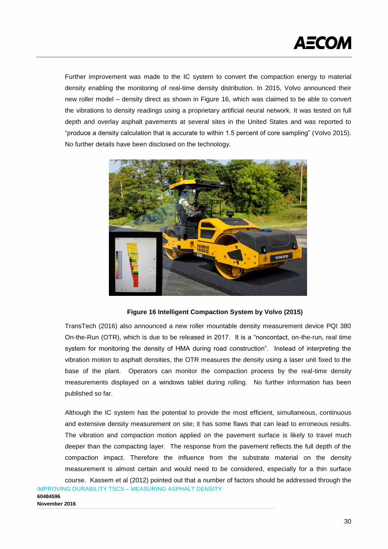
Further improvement was made to the IC system to convert the compaction energy to material
density enabling the monitoring of real-time density distribution. In 2015, Volvo announced their
new roller model – density direct as shown in Figure 16, which was claimed to be able to convert
the vibrations to density readings using a proprietary artificial neural network. It was tested on full
depth and overlay asphalt pavements at several sites in the United States and was reported to
“produce a density calculation that is accurate to within 1.5 percent of core sampling” (Volvo 2015).
No further details have been disclosed on the technology.
Figure 16 Intelligent Compaction System by Volvo (2015)
TransTech (2016) also announced a new roller mountable density measurement device PQI 380
On-the-Run (OTR), which is due to be released in 2017. It is a “noncontact, on-the-run, real time
system for monitoring the density of HMA during road construction”. Instead of interpreting the
vibration motion to asphalt densities, the OTR measures the density using a laser unit fixed to the
base of the plant. Operators can monitor the compaction process by the real-time density
measurements displayed on a windows tablet during rolling. No further information has been
published so far.
Although the IC system has the potential to provide the most efficient, simultaneous, continuous
and extensive density measurement on site; it has some flaws that can lead to erroneous results.
The vibration and compaction motion applied on the pavement surface is likely to travel much
deeper than the compacting layer. The response from the pavement reflects the full depth of the
compaction impact. Therefore the influence from the substrate material on the density
measurement is almost certain and would need to be considered, especially for a thin surface
course. Kassem et al (2012) pointed out that a number of factors should be addressed through the
IMPROVING DURABILITY TSCS – MEASURING ASPHALT DENSITY
60484596
November 2016
31
calibration process and fed into a software programme which could potentially interpret the
compaction behaviour into the material density. The following factors were considered by Kassem
et al (2012) – mix surface temperatures and the temperature gradient through depths, roller
passes, compaction energy distribution along a roller drum, roller compactor types and operation
modes. The abovementioned issue with lift thickness and underlying material was not discussed in
the proposal.
The emerging technology on roller mounted asphalt density devices has the potential to become
the future trend in non-destructive density measurement. However, it still faces some challenges
such as the effect of the underlying material and lack of guidance on the calibration and precision
level. Therefore, it is considered that there is not sufficient evidence to prove its suitability to use
on TSCS at this stage.
4. RECOMMENDATIONS
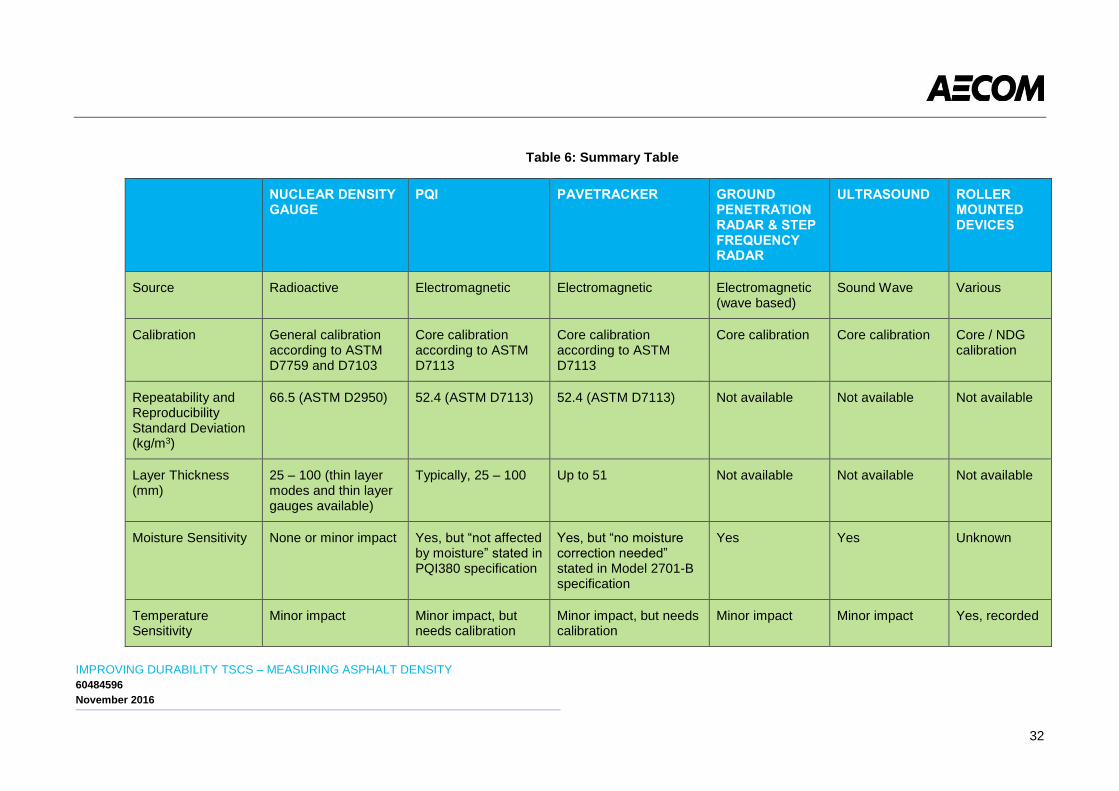
The reviewed methods are summarised in Table 6 below according to their attributes to help
selecting the appropriate methods for in-situ trials. The core density is the only direct measurement
of the density and is used as the calibration reference. Hence it is not included in the comparison.
The electromagnetic wave based method, GPR and SFR, and the ultrasound method are still at
the research stage and in need of further investigations. The intelligent compaction system has
been used for quality control for over 20 years, but its application in density measurement is very
recent and has not been fully comprehended by the industry. Although the roller compactor with
the ability to measure asphalt density is now available commercially, there are questions regarding
the soundness of the results. Further evaluation is required to decide the measuring layer
thickness and the measurement precision. The nuclear gauge method and capacitive
electromagnetic method have been established for in-situ density measurements for long time.
There are extensive standards and guidance for their calibrations, operations and precision levels
in the ASTM documents. The British standards also offer some guidance. According to the
literature, the sensitivity to moisture of PQI and PaveTracker was high and their precision levels
were more acceptable for QC than for QA. However, early models of devices were used in most of
the literature. New models are expected to perform better. More options are provided for various
lift thicknesses in new models. Based on the above, it is recommended to further explore the
potentials for using non-nuclear capacitive electromagnetic equipment, such as PaveTracker, for
QA/QC in situ density assessments of TSCS.
IMPROVING DURABILITY TSCS – MEASURING ASPHALT DENSITY
60484596
November 2016
32
Table 6: Summary Table
NUCLEAR DENSITY GAUGE
PQI PAVETRACKER GROUND PENETRATION RADAR & STEP FREQUENCY RADAR
ULTRASOUND ROLLER MOUNTED DEVICES
Source Radioactive Electromagnetic Electromagnetic Electromagnetic (wave based)
Sound Wave Various
Calibration General calibration according to ASTM D7759 and D7103
Core calibration according to ASTM D7113
Core calibration according to ASTM D7113
Core calibration Core calibration Core / NDG calibration
Repeatability and Reproducibility Standard Deviation (kg/m3)
66.5 (ASTM D2950) 52.4 (ASTM D7113) 52.4 (ASTM D7113) Not available Not available Not available
Layer Thickness (mm)
25 – 100 (thin layer modes and thin layer gauges available)
Typically, 25 – 100 Up to 51 Not available Not available Not available
Moisture Sensitivity None or minor impact Yes, but “not affected by moisture” stated in PQI380 specification
Yes, but “no moisture correction needed” stated in Model 2701-B specification
Yes Yes Unknown
Temperature Sensitivity
Minor impact Minor impact, but needs calibration
Minor impact, but needs calibration
Minor impact Minor impact Yes, recorded
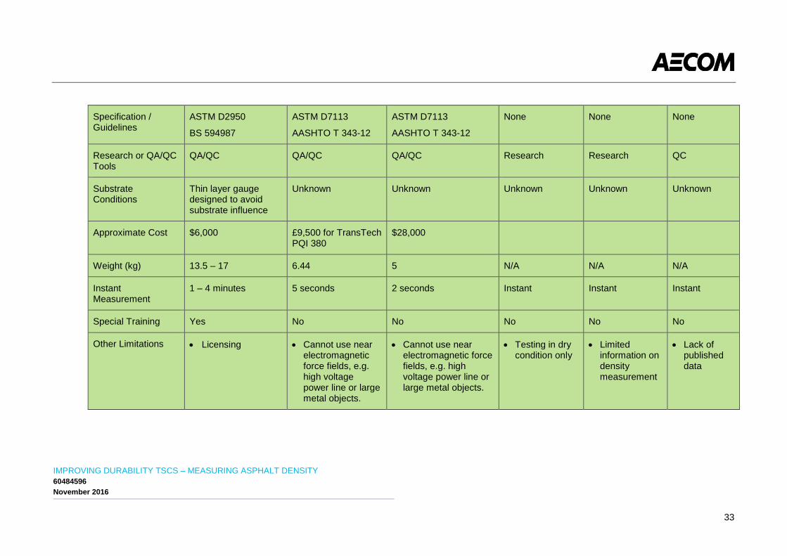
IMPROVING DURABILITY TSCS – MEASURING ASPHALT DENSITY
60484596
November 2016
33
Specification / Guidelines
ASTM D2950
BS 594987
ASTM D7113
AASHTO T 343-12
ASTM D7113
AASHTO T 343-12
None None None
Research or QA/QC Tools
QA/QC QA/QC QA/QC Research Research QC
Substrate Conditions
Thin layer gauge designed to avoid substrate influence
Unknown Unknown Unknown Unknown Unknown
Approximate Cost $6,000 £9,500 for TransTech PQI 380
$28,000
Weight (kg) 13.5 – 17 6.44 5 N/A N/A N/A
Instant Measurement
1 – 4 minutes 5 seconds 2 seconds Instant Instant Instant
Special Training Yes No No No No No
Other Limitations Licensing Cannot use near electromagnetic force fields, e.g. high voltage power line or large metal objects.
Cannot use near electromagnetic force fields, e.g. high voltage power line or large metal objects.
Testing in dry condition only
Limited information on density measurement
Lack of published data
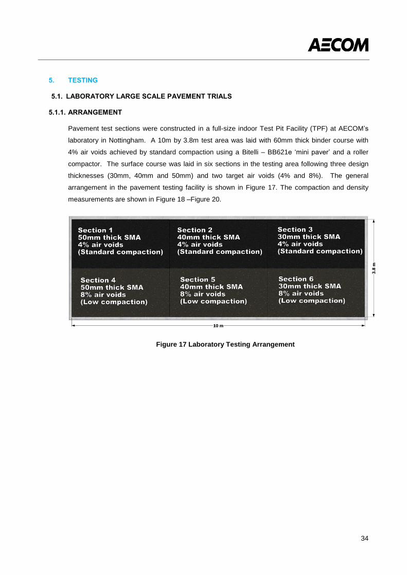
34
5. TESTING
5.1. LABORATORY LARGE SCALE PAVEMENT TRIALS
5.1.1. ARRANGEMENT
Pavement test sections were constructed in a full-size indoor Test Pit Facility (TPF) at AECOM’s
laboratory in Nottingham. A 10m by 3.8m test area was laid with 60mm thick binder course with
4% air voids achieved by standard compaction using a Bitelli – BB621e ‘mini paver’ and a roller
compactor. The surface course was laid in six sections in the testing area following three design
thicknesses (30mm, 40mm and 50mm) and two target air voids (4% and 8%). The general
arrangement in the pavement testing facility is shown in Figure 17. The compaction and density
measurements are shown in Figure 18 –Figure 20.
Figure 17 Laboratory Testing Arrangement
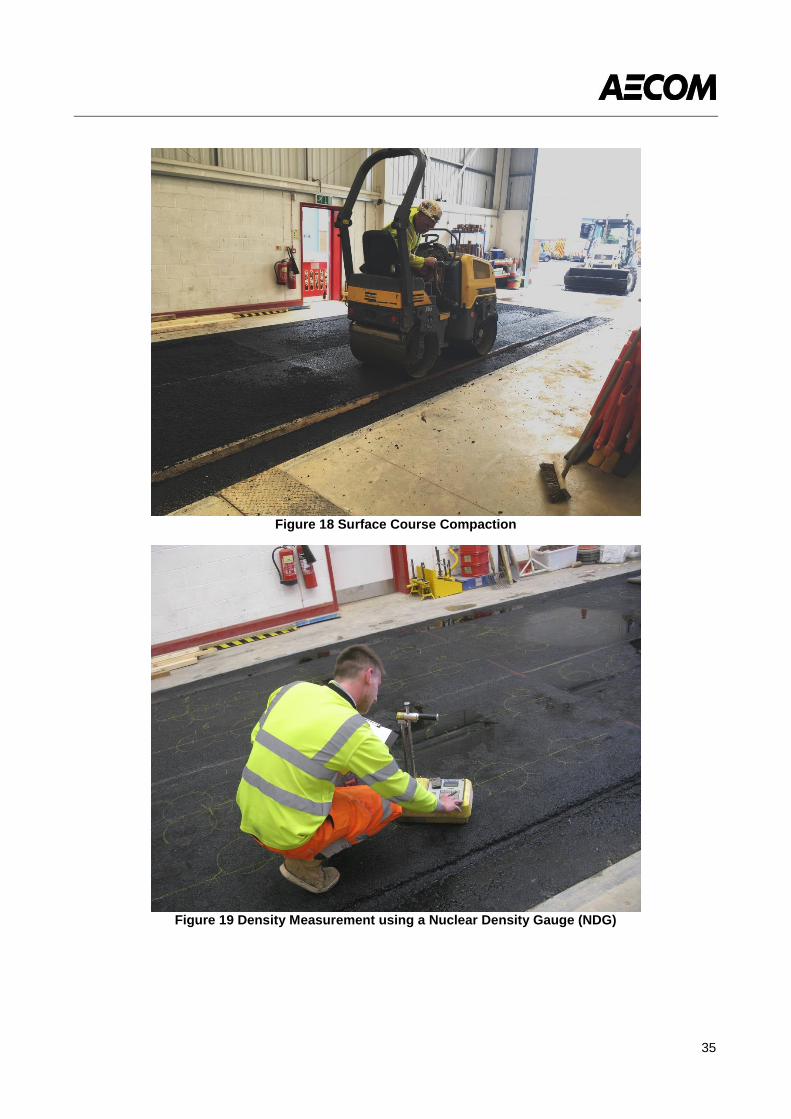
35
Figure 18 Surface Course Compaction
Figure 19 Density Measurement using a Nuclear Density Gauge (NDG)
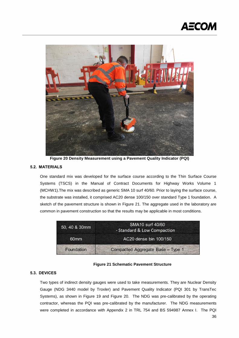
36
Figure 20 Density Measurement using a Pavement Quality Indicator (PQI)
5.2. MATERIALS
One standard mix was developed for the surface course according to the Thin Surface Course
Systems (TSCS) in the Manual of Contract Documents for Highway Works Volume 1
(MCHW1).The mix was described as generic SMA 10 surf 40/60. Prior to laying the surface course,
the substrate was installed, it comprised AC20 dense 100/150 over standard Type 1 foundation. A
sketch of the pavement structure is shown in Figure 21. The aggregate used in the laboratory are
common in pavement construction so that the results may be applicable in most conditions.
Figure 21 Schematic Pavement Structure
5.3. DEVICES
Two types of indirect density gauges were used to take measurements. They are Nuclear Density
Gauge (NDG 3440 model by Troxler) and Pavement Quality Indicator (PQI 301 by TransTec
Systems), as shown in Figure 19 and Figure 20. The NDG was pre-calibrated by the operating
contractor, whereas the PQI was pre-calibrated by the manufacturer. The NDG measurements
were completed in accordance with Appendix 2 in TRL 754 and BS 594987 Annex I. The PQI
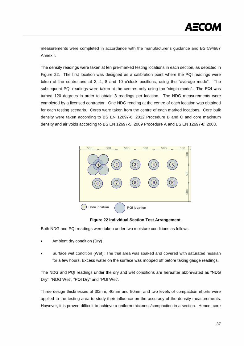
37
measurements were completed in accordance with the manufacturer’s guidance and BS 594987
Annex I.
The density readings were taken at ten pre-marked testing locations in each section, as depicted in
Figure 22. The first location was designed as a calibration point where the PQI readings were
taken at the centre and at 2, 4, 8 and 10 o’clock positions, using the “average mode”. The
subsequent PQI readings were taken at the centres only using the “single mode”. The PQI was
turned 120 degrees in order to obtain 3 readings per location. The NDG measurements were
completed by a licensed contractor. One NDG reading at the centre of each location was obtained
for each testing scenario. Cores were taken from the centre of each marked locations. Core bulk
density were taken according to BS EN 12697-6: 2012 Procedure B and C and core maximum
density and air voids according to BS EN 12697-5: 2009 Procedure A and BS EN 12697-8: 2003.
Figure 22 Individual Section Test Arrangement
Both NDG and PQI readings were taken under two moisture conditions as follows.
Ambient dry condition (Dry)
Surface wet condition (Wet): The trial area was soaked and covered with saturated hessian
for a few hours. Excess water on the surface was mopped off before taking gauge readings.
The NDG and PQI readings under the dry and wet conditions are hereafter abbreviated as “NDG
Dry”, “NDG Wet”, “PQI Dry” and “PQI Wet”.
Three design thicknesses of 30mm, 40mm and 50mm and two levels of compaction efforts were
applied to the testing area to study their influence on the accuracy of the density measurements.
However, it is proved difficult to achieve a uniform thickness/compaction in a section. Hence, core
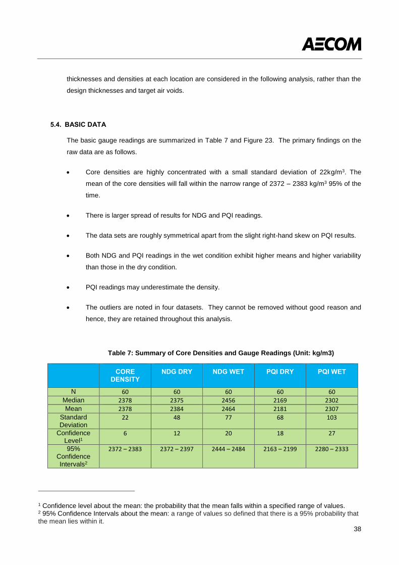
38
thicknesses and densities at each location are considered in the following analysis, rather than the
design thicknesses and target air voids.
5.4. BASIC DATA
The basic gauge readings are summarized in Table 7 and Figure 23. The primary findings on the
raw data are as follows.
Core densities are highly concentrated with a small standard deviation of 22kg/m3. The
mean of the core densities will fall within the narrow range of 2372 – 2383 kg/m3 95% of the
time.
There is larger spread of results for NDG and PQI readings.
The data sets are roughly symmetrical apart from the slight right-hand skew on PQI results.
Both NDG and PQI readings in the wet condition exhibit higher means and higher variability
than those in the dry condition.
PQI readings may underestimate the density.
The outliers are noted in four datasets. They cannot be removed without good reason and
hence, they are retained throughout this analysis.
Table 7: Summary of Core Densities and Gauge Readings (Unit: kg/m3)
CORE DENSITY
NDG DRY NDG WET PQI DRY PQI WET
N 60 60 60 60 60
Median 2378 2375 2456 2169 2302
Mean 2378 2384 2464 2181 2307
Standard Deviation
22 48 77 68 103
Confidence Level1
6 12 20 18 27
95% Confidence Intervals2
2372 – 2383 2372 – 2397 2444 – 2484 2163 – 2199 2280 – 2333
1 Confidence level about the mean: the probability that the mean falls within a specified range of values. 2 95% Confidence Intervals about the mean: a range of values so defined that there is a 95% probability that the mean lies within it.
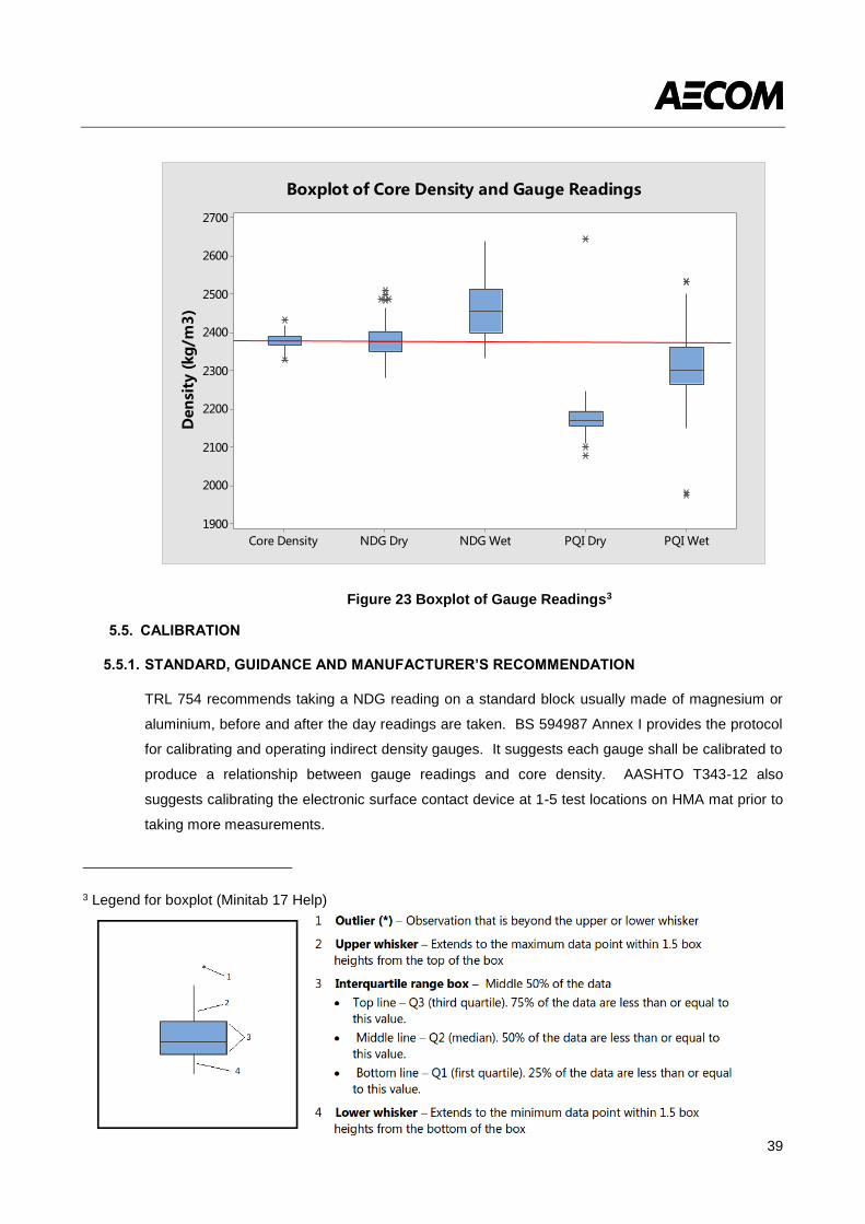
39
Figure 23 Boxplot of Gauge Readings3
5.5. CALIBRATION
5.5.1. STANDARD, GUIDANCE AND MANUFACTURER’S RECOMMENDATION
TRL 754 recommends taking a NDG reading on a standard block usually made of magnesium or
aluminium, before and after the day readings are taken. BS 594987 Annex I provides the protocol
for calibrating and operating indirect density gauges. It suggests each gauge shall be calibrated to
produce a relationship between gauge readings and core density. AASHTO T343-12 also
suggests calibrating the electronic surface contact device at 1-5 test locations on HMA mat prior to
taking more measurements.
3 Legend for boxplot (Minitab 17 Help)
PQI WetPQI DryNDG WetNDG DryCore Density
2700
2600
2500
2400
2300
2200
2100
2000
1900
Den
sity
(kg
/m3
)Boxplot of Core Density and Gauge Readings
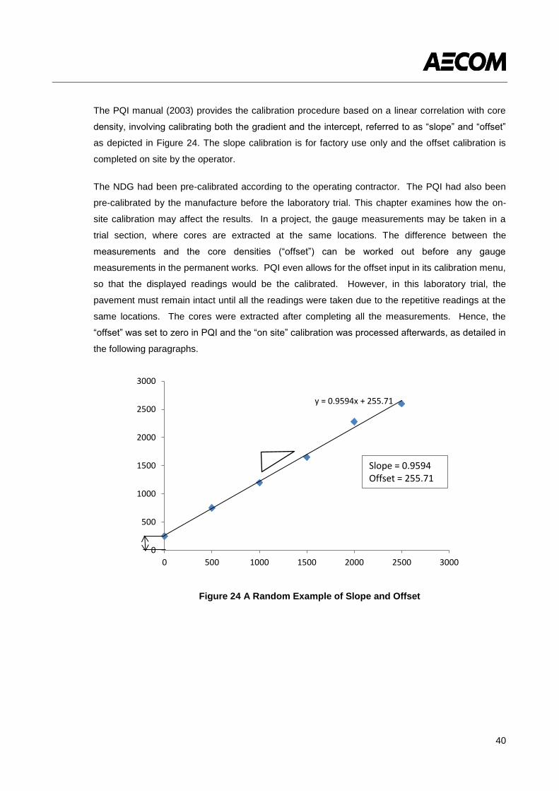
40
The PQI manual (2003) provides the calibration procedure based on a linear correlation with core
density, involving calibrating both the gradient and the intercept, referred to as “slope” and “offset”
as depicted in Figure 24. The slope calibration is for factory use only and the offset calibration is
completed on site by the operator.
The NDG had been pre-calibrated according to the operating contractor. The PQI had also been
pre-calibrated by the manufacture before the laboratory trial. This chapter examines how the on-
site calibration may affect the results. In a project, the gauge measurements may be taken in a
trial section, where cores are extracted at the same locations. The difference between the
measurements and the core densities (“offset”) can be worked out before any gauge
measurements in the permanent works. PQI even allows for the offset input in its calibration menu,
so that the displayed readings would be the calibrated. However, in this laboratory trial, the
pavement must remain intact until all the readings were taken due to the repetitive readings at the
same locations. The cores were extracted after completing all the measurements. Hence, the
“offset” was set to zero in PQI and the “on site” calibration was processed afterwards, as detailed in
the following paragraphs.
Figure 24 A Random Example of Slope and Offset
y = 0.9594x + 255.71
0
500
1000
1500
2000
2500
3000
0 500 1000 1500 2000 2500 3000
Slope = 0.9594Offset = 255.71
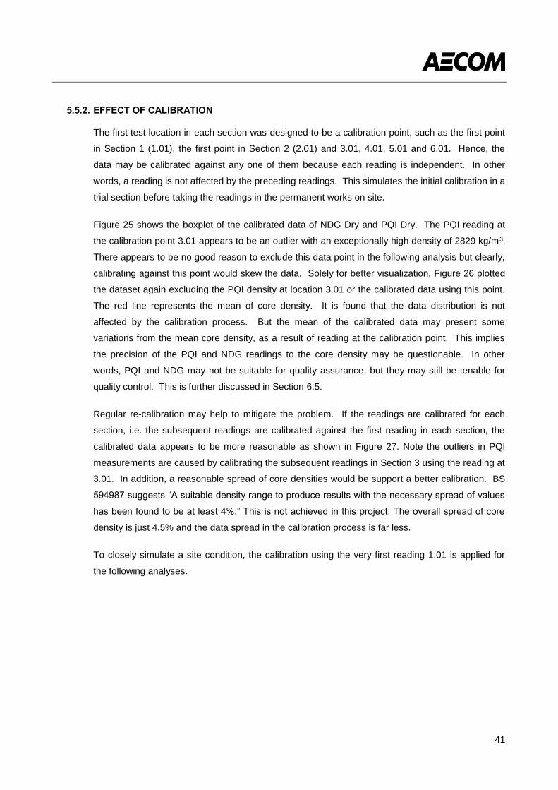
41
5.5.2. EFFECT OF CALIBRATION
The first test location in each section was designed to be a calibration point, such as the first point
in Section 1 (1.01), the first point in Section 2 (2.01) and 3.01, 4.01, 5.01 and 6.01. Hence, the
data may be calibrated against any one of them because each reading is independent. In other
words, a reading is not affected by the preceding readings. This simulates the initial calibration in a
trial section before taking the readings in the permanent works on site.
Figure 25 shows the boxplot of the calibrated data of NDG Dry and PQI Dry. The PQI reading at
the calibration point 3.01 appears to be an outlier with an exceptionally high density of 2829 kg/m3.
There appears to be no good reason to exclude this data point in the following analysis but clearly,
calibrating against this point would skew the data. Solely for better visualization, Figure 26 plotted
the dataset again excluding the PQI density at location 3.01 or the calibrated data using this point.
The red line represents the mean of core density. It is found that the data distribution is not
affected by the calibration process. But the mean of the calibrated data may present some
variations from the mean core density, as a result of reading at the calibration point. This implies
the precision of the PQI and NDG readings to the core density may be questionable. In other
words, PQI and NDG may not be suitable for quality assurance, but they may still be tenable for
quality control. This is further discussed in Section 6.5.
Regular re-calibration may help to mitigate the problem. If the readings are calibrated for each
section, i.e. the subsequent readings are calibrated against the first reading in each section, the
calibrated data appears to be more reasonable as shown in Figure 27. Note the outliers in PQI
measurements are caused by calibrating the subsequent readings in Section 3 using the reading at
3.01. In addition, a reasonable spread of core densities would be support a better calibration. BS
594987 suggests “A suitable density range to produce results with the necessary spread of values
has been found to be at least 4%.” This is not achieved in this project. The overall spread of core
density is just 4.5% and the data spread in the calibration process is far less.
To closely simulate a site condition, the calibration using the very first reading 1.01 is applied for
the following analyses.
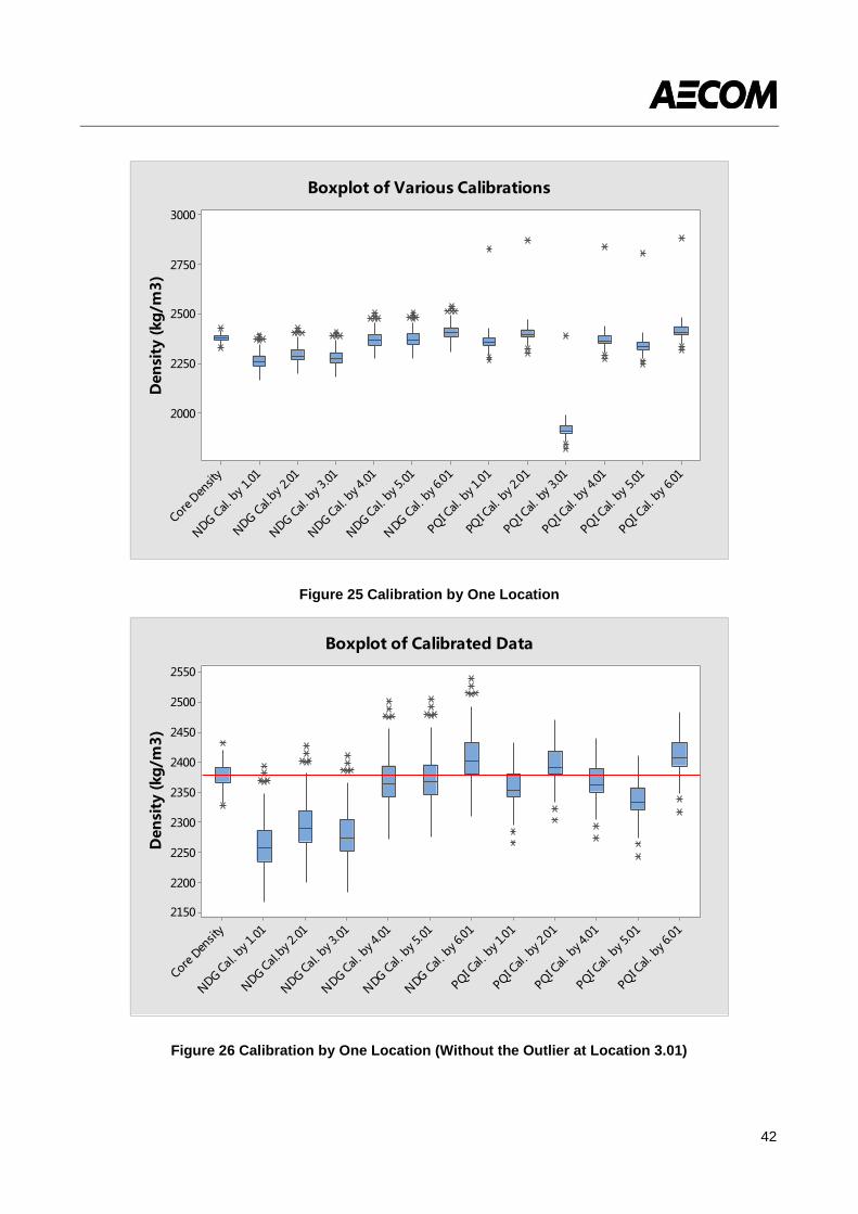
42
Figure 25 Calibration by One Location
Figure 26 Calibration by One Location (Without the Outlier at Location 3.01)
PQI C
al. b
y 6.01
PQI C
al. b
y 5.01
PQI C
al. b
y 4.01
PQI C
al. b
y 3.01
PQI C
al. b
y 2.01
PQI C
al. b
y 1.01
NDG
Cal
. by 6.01
NDG
Cal.
by 5.
01
NDG
Cal.
by 4.0
1
NDG
Cal. b
y 3.0
1
NDG
Cal.b
y 2.01
NDG
Cal. b
y 1.01
Core D
ensity
3000
2750
2500
2250
2000
Den
sity
(kg
/m3
)
Boxplot of Various Calibrations
PQI C
al. b
y 6.01
PQI C
al. b
y 5.01
PQI C
al. b
y 4.01
PQI C
al. b
y 2.01
PQI C
al. b
y 1.01
NDG
Cal
. by 6.01
NDG
Cal
. by 5.
01
NDG
Cal
. by 4.
01
NDG
Cal.
by 3.
01
NDG
Cal.b
y 2.
01
NDG
Cal.
by 1.
01
Core D
ensity
2550
2500
2450
2400
2350
2300
2250
2200
2150
Den
sity
(kg
/m3
)
Boxplot of Calibrated Data
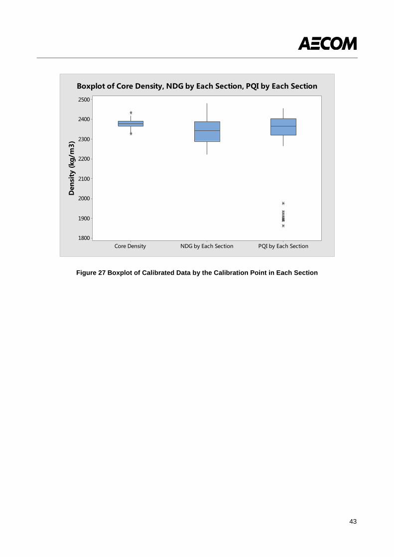
43
Figure 27 Boxplot of Calibrated Data by the Calibration Point in Each Section
PQI by Each SectionNDG by Each SectionCore Density
2500
2400
2300
2200
2100
2000
1900
1800
Den
sity
(kg
/m3
)
Boxplot of Core Density, NDG by Each Section, PQI by Each Section
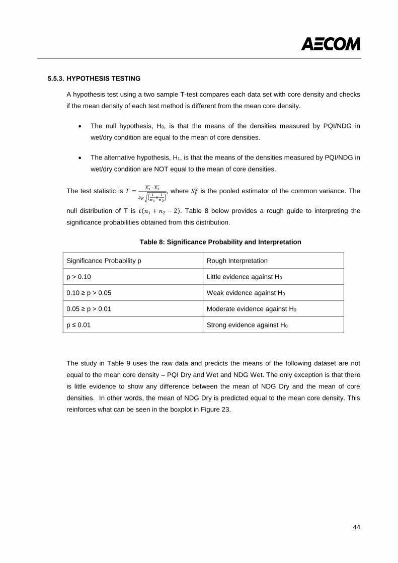
44
5.5.3. HYPOTHESIS TESTING
A hypothesis test using a two sample T-test compares each data set with core density and checks
if the mean density of each test method is different from the mean core density.
The null hypothesis, H0, is that the means of the densities measured by PQI/NDG in
wet/dry condition are equal to the mean of core densities.
The alternative hypothesis, H1, is that the means of the densities measured by PQI/NDG in
wet/dry condition are NOT equal to the mean of core densities.
The test statistic is 𝑇 =𝑋1̅̅ ̅̅ −𝑋2̅̅ ̅̅
𝑆𝑃√(1
𝑛1+
1
𝑛2), where 𝑆𝑃
2 is the pooled estimator of the common variance. The
null distribution of T is 𝑡(𝑛1 + 𝑛2 − 2). Table 8 below provides a rough guide to interpreting the
significance probabilities obtained from this distribution.
Table 8: Significance Probability and Interpretation
Significance Probability p Rough Interpretation
p > 0.10 Little evidence against H0
0.10 ≥ p > 0.05 Weak evidence against H0
0.05 ≥ p > 0.01 Moderate evidence against H0
p ≤ 0.01 Strong evidence against H0
The study in Table 9 uses the raw data and predicts the means of the following dataset are not
equal to the mean core density – PQI Dry and Wet and NDG Wet. The only exception is that there
is little evidence to show any difference between the mean of NDG Dry and the mean of core
densities. In other words, the mean of NDG Dry is predicted equal to the mean core density. This
reinforces what can be seen in the boxplot in Figure 23.
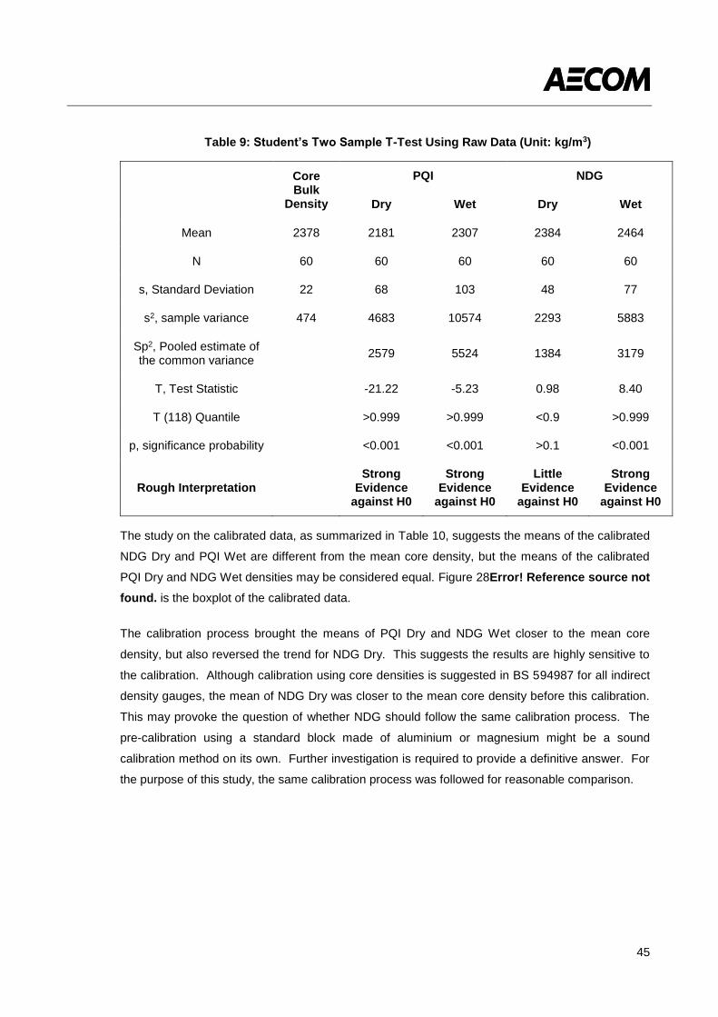
45
Table 9: Student’s Two Sample T-Test Using Raw Data (Unit: kg/m3)
Core Bulk
Density
PQI NDG
Dry Wet Dry Wet
Mean 2378 2181 2307 2384 2464
N 60 60 60 60 60
s, Standard Deviation 22 68 103 48 77
s2, sample variance 474 4683 10574 2293 5883
Sp2, Pooled estimate of the common variance
2579 5524 1384 3179
T, Test Statistic -21.22 -5.23 0.98 8.40
T (118) Quantile >0.999 >0.999 <0.9 >0.999
p, significance probability <0.001 <0.001 >0.1 <0.001
Rough Interpretation Strong
Evidence against H0
Strong Evidence
against H0
Little Evidence
against H0
Strong Evidence
against H0
The study on the calibrated data, as summarized in Table 10, suggests the means of the calibrated
NDG Dry and PQI Wet are different from the mean core density, but the means of the calibrated
PQI Dry and NDG Wet densities may be considered equal. Figure 28Error! Reference source not
found. is the boxplot of the calibrated data.
The calibration process brought the means of PQI Dry and NDG Wet closer to the mean core
density, but also reversed the trend for NDG Dry. This suggests the results are highly sensitive to
the calibration. Although calibration using core densities is suggested in BS 594987 for all indirect
density gauges, the mean of NDG Dry was closer to the mean core density before this calibration.
This may provoke the question of whether NDG should follow the same calibration process. The
pre-calibration using a standard block made of aluminium or magnesium might be a sound
calibration method on its own. Further investigation is required to provide a definitive answer. For
the purpose of this study, the same calibration process was followed for reasonable comparison.
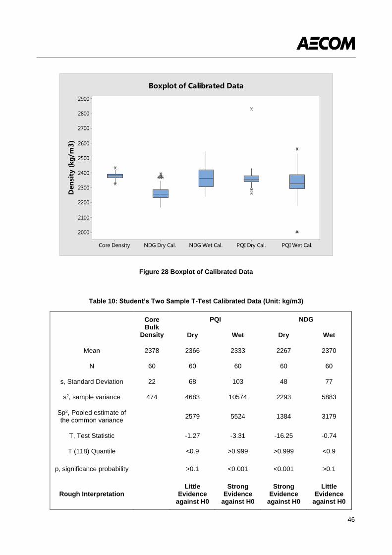
46
Figure 28 Boxplot of Calibrated Data
Table 10: Student’s Two Sample T-Test Calibrated Data (Unit: kg/m3)
Core Bulk
Density
PQI NDG
Dry Wet Dry Wet
Mean 2378 2366 2333 2267 2370
N 60 60 60 60 60
s, Standard Deviation 22 68 103 48 77
s2, sample variance 474 4683 10574 2293 5883
Sp2, Pooled estimate of the common variance
2579 5524 1384 3179
T, Test Statistic -1.27 -3.31 -16.25 -0.74
T (118) Quantile <0.9 >0.999 >0.999 <0.9
p, significance probability >0.1 <0.001 <0.001 >0.1
Rough Interpretation Little
Evidence against H0
Strong Evidence
against H0
Strong Evidence
against H0
Little Evidence
against H0
PQI Wet Cal.PQI Dry Cal.NDG Wet Cal.NDG Dry Cal.Core Density
2900
2800
2700
2600
2500
2400
2300
2200
2100
2000
Den
sity
(kg
/m3
)
Boxplot of Calibrated Data
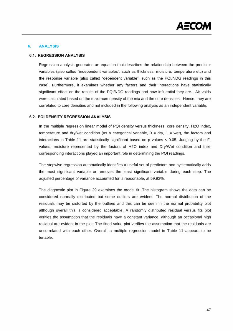
47
6. ANALYSIS
6.1. REGRESSION ANALYSIS
Regression analysis generates an equation that describes the relationship between the predictor
variables (also called “independent variables”, such as thickness, moisture, temperature etc) and
the response variable (also called “dependent variable”, such as the PQI/NDG readings in this
case). Furthermore, it examines whether any factors and their interactions have statistically
significant effect on the results of the PQI/NDG readings and how influential they are. Air voids
were calculated based on the maximum density of the mix and the core densities. Hence, they are
correlated to core densities and not included in the following analysis as an independent variable.
6.2. PQI DENSITY REGRESSION ANALYSIS
In the multiple regression linear model of PQI density versus thickness, core density, H2O index,
temperature and dry/wet condition (as a categorical variable, 0 = dry, 1 = wet), the factors and
interactions in Table 11 are statistically significant based on p values < 0.05. Judging by the F-
values, moisture represented by the factors of H2O index and Dry/Wet condition and their
corresponding interactions played an important role in determining the PQI readings.
The stepwise regression automatically identifies a useful set of predictors and systematically adds
the most significant variable or removes the least significant variable during each step. The
adjusted percentage of variance accounted for is reasonable, at 59.92%.
The diagnostic plot in Figure 29 examines the model fit. The histogram shows the data can be
considered normally distributed but some outliers are evident. The normal distribution of the
residuals may be distorted by the outliers and this can be seen in the normal probability plot
although overall this is considered acceptable. A randomly distributed residual versus fits plot
verifies the assumption that the residuals have a constant variance, although an occasional high
residual are evident in the plot. The fitted value plot verifies the assumption that the residuals are
uncorrelated with each other. Overall, a multiple regression model in Table 11 appears to be
tenable.
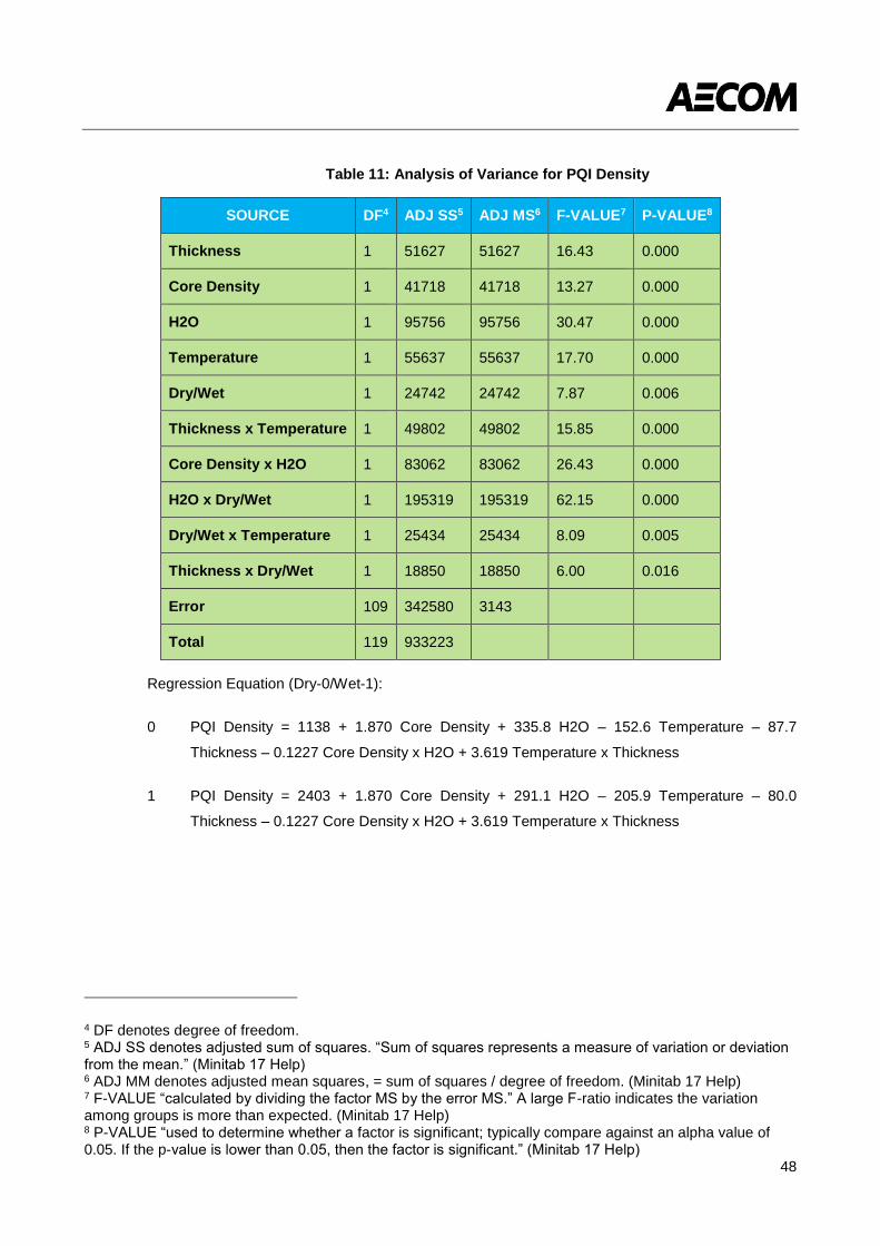
48
Table 11: Analysis of Variance for PQI Density
SOURCE DF4 ADJ SS5 ADJ MS6 F-VALUE7 P-VALUE8
Thickness 1 51627 51627 16.43 0.000
Core Density 1 41718 41718 13.27 0.000
H2O 1 95756 95756 30.47 0.000
Temperature 1 55637 55637 17.70 0.000
Dry/Wet 1 24742 24742 7.87 0.006
Thickness x Temperature 1 49802 49802 15.85 0.000
Core Density x H2O 1 83062 83062 26.43 0.000
H2O x Dry/Wet 1 195319 195319 62.15 0.000
Dry/Wet x Temperature 1 25434 25434 8.09 0.005
Thickness x Dry/Wet 1 18850 18850 6.00 0.016
Error 109 342580 3143
Total 119 933223
Regression Equation (Dry-0/Wet-1):
0 PQI Density = 1138 + 1.870 Core Density + 335.8 H2O – 152.6 Temperature – 87.7
Thickness – 0.1227 Core Density x H2O + 3.619 Temperature x Thickness
1 PQI Density = 2403 + 1.870 Core Density + 291.1 H2O – 205.9 Temperature – 80.0
Thickness – 0.1227 Core Density x H2O + 3.619 Temperature x Thickness
4 DF denotes degree of freedom. 5 ADJ SS denotes adjusted sum of squares. “Sum of squares represents a measure of variation or deviation from the mean.” (Minitab 17 Help) 6 ADJ MM denotes adjusted mean squares, = sum of squares / degree of freedom. (Minitab 17 Help) 7 F-VALUE “calculated by dividing the factor MS by the error MS.” A large F-ratio indicates the variation among groups is more than expected. (Minitab 17 Help) 8 P-VALUE “used to determine whether a factor is significant; typically compare against an alpha value of 0.05. If the p-value is lower than 0.05, then the factor is significant.” (Minitab 17 Help)
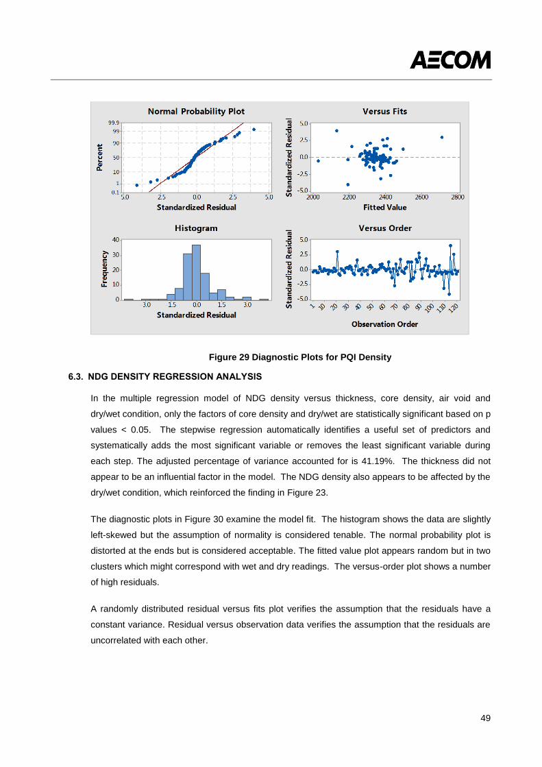
49
Figure 29 Diagnostic Plots for PQI Density
6.3. NDG DENSITY REGRESSION ANALYSIS
In the multiple regression model of NDG density versus thickness, core density, air void and
dry/wet condition, only the factors of core density and dry/wet are statistically significant based on p
values < 0.05. The stepwise regression automatically identifies a useful set of predictors and
systematically adds the most significant variable or removes the least significant variable during
each step. The adjusted percentage of variance accounted for is 41.19%. The thickness did not
appear to be an influential factor in the model. The NDG density also appears to be affected by the
dry/wet condition, which reinforced the finding in Figure 23.
The diagnostic plots in Figure 30 examine the model fit. The histogram shows the data are slightly
left-skewed but the assumption of normality is considered tenable. The normal probability plot is
distorted at the ends but is considered acceptable. The fitted value plot appears random but in two
clusters which might correspond with wet and dry readings. The versus-order plot shows a number
of high residuals.
A randomly distributed residual versus fits plot verifies the assumption that the residuals have a
constant variance. Residual versus observation data verifies the assumption that the residuals are
uncorrelated with each other.
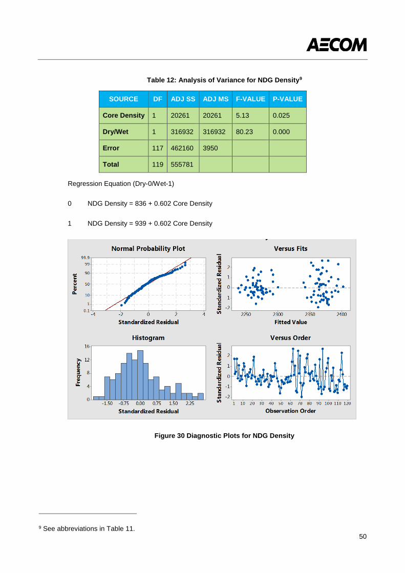
50
Table 12: Analysis of Variance for NDG Density9
SOURCE DF ADJ SS ADJ MS F-VALUE P-VALUE
Core Density 1 20261 20261 5.13 0.025
Dry/Wet 1 316932 316932 80.23 0.000
Error 117 462160 3950
Total 119 555781
Regression Equation (Dry-0/Wet-1)
0 NDG Density = 836 + 0.602 Core Density
1 NDG Density = 939 + 0.602 Core Density
Figure 30 Diagnostic Plots for NDG Density
9 See abbreviations in Table 11.
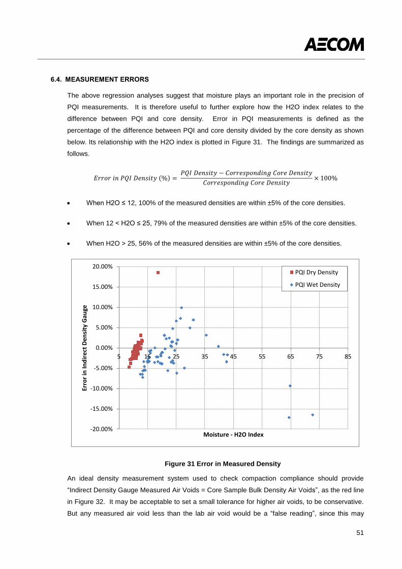
51
6.4. MEASUREMENT ERRORS
The above regression analyses suggest that moisture plays an important role in the precision of
PQI measurements. It is therefore useful to further explore how the H2O index relates to the
difference between PQI and core density. Error in PQI measurements is defined as the
percentage of the difference between PQI and core density divided by the core density as shown
below. Its relationship with the H2O index is plotted in Figure 31. The findings are summarized as
follows.
𝐸𝑟𝑟𝑜𝑟 𝑖𝑛 𝑃𝑄𝐼 𝐷𝑒𝑛𝑠𝑖𝑡𝑦 (%) = 𝑃𝑄𝐼 𝐷𝑒𝑛𝑠𝑖𝑡𝑦 − 𝐶𝑜𝑟𝑟𝑒𝑠𝑝𝑜𝑛𝑑𝑖𝑛𝑔 𝐶𝑜𝑟𝑒 𝐷𝑒𝑛𝑠𝑖𝑡𝑦
𝐶𝑜𝑟𝑟𝑒𝑠𝑝𝑜𝑛𝑑𝑖𝑛𝑔 𝐶𝑜𝑟𝑒 𝐷𝑒𝑛𝑠𝑖𝑡𝑦× 100%
When H2O ≤ 12, 100% of the measured densities are within ±5% of the core densities.
When 12 < H2O ≤ 25, 79% of the measured densities are within ±5% of the core densities.
When H2O > 25, 56% of the measured densities are within ±5% of the core densities.
Figure 31 Error in Measured Density
An ideal density measurement system used to check compaction compliance should provide
“Indirect Density Gauge Measured Air Voids = Core Sample Bulk Density Air Voids”, as the red line
in Figure 32. It may be acceptable to set a small tolerance for higher air voids, to be conservative.
But any measured air void less than the lab air void would be a “false reading”, since this may
-20.00%
-15.00%
-10.00%
-5.00%
0.00%
5.00%
10.00%
15.00%
20.00%
5 15 25 35 45 55 65 75 85
Erro
r in
Ind
ire
ct D
en
sity
Gau
ge
Moisture - H2O Index
PQI Dry Density
PQI Wet Density
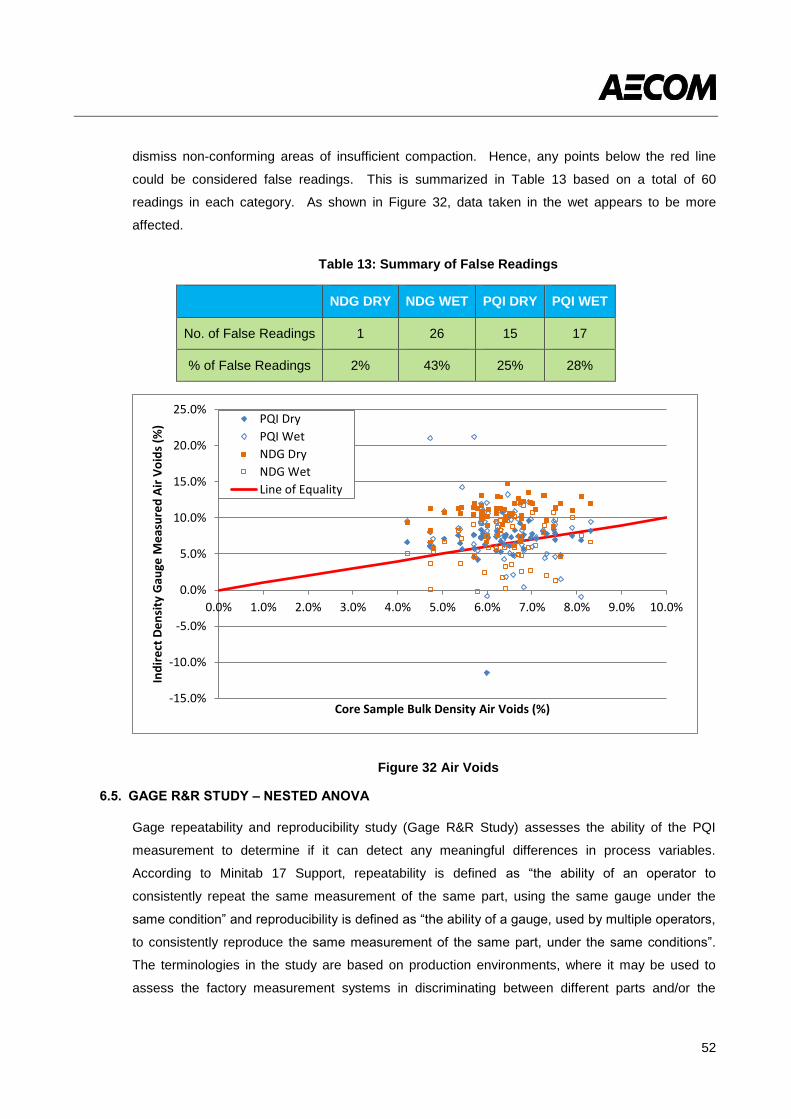
52
dismiss non-conforming areas of insufficient compaction. Hence, any points below the red line
could be considered false readings. This is summarized in Table 13 based on a total of 60
readings in each category. As shown in Figure 32, data taken in the wet appears to be more
affected.
Table 13: Summary of False Readings
NDG DRY NDG WET PQI DRY PQI WET
No. of False Readings 1 26 15 17
% of False Readings 2% 43% 25% 28%
Figure 32 Air Voids
6.5. GAGE R&R STUDY – NESTED ANOVA
Gage repeatability and reproducibility study (Gage R&R Study) assesses the ability of the PQI
measurement to determine if it can detect any meaningful differences in process variables.
According to Minitab 17 Support, repeatability is defined as “the ability of an operator to
consistently repeat the same measurement of the same part, using the same gauge under the
same condition” and reproducibility is defined as “the ability of a gauge, used by multiple operators,
to consistently reproduce the same measurement of the same part, under the same conditions”.
The terminologies in the study are based on production environments, where it may be used to
assess the factory measurement systems in discriminating between different parts and/or the
-15.0%
-10.0%
-5.0%
0.0%
5.0%
10.0%
15.0%
20.0%
25.0%
0.0% 1.0% 2.0% 3.0% 4.0% 5.0% 6.0% 7.0% 8.0% 9.0% 10.0%
Ind
ire
ct D
en
sity
Gau
ge M
eas
ure
d A
ir V
oid
s (%
)
Core Sample Bulk Density Air Voids (%)
PQI Dry
PQI Wet
NDG Dry
NDG Wet
Line of Equality
53
variability caused by different operators. In our case, “part” means testing location. “Part-To-Part”
represents from the density variation from one testing location to another.
Three repeated readings were taken at 54 testing locations (excluding the calibration points in each
section). Although only two operators were involved in the test, each section was assumed to have
a different operator to balance the study. The assessment of the reproducibility is not valid and
was discarded, but the repeatability was considered valid. The “Total Gage R&R” is considered as
the performance of the overall measurement system with primary contribution from repeatability.
The NDG measurements were taken by others and only the averaged reading at each location was
provided. Hence, the NDG measurements cannot be assessed for the R&R.
There are two main types of gage R&R – crossed and nested. In this case, the nested study is
applicable.
Gage R&R Study (Crossed): The same samples are repeatedly measured by independent
operators,
Gage R&R Study (Nested): The samples are measured by one assigned operator only.
Figure 33 and Table 15 summarize the analysis results. Looking at the %Contribution columns for
Total Gage R&R and Part-to-Part, it can be seen that the percent contribution for differences
between parts (Part-To-Part = 96.43) is much larger than the percentage contribution for
measurement system variation (Total Gage R&R = 3.57). The %Study Var column indicates that
the Total Gage R&R equals 18.90% of the study variation and the Part-To-Part equals 98.20% of
the study variation. Hence, most of the variation is due to differences between testing locations and
little is due to measurement system errors.
An important index is the number of different categories, which estimates how many separate
groups of samples the system can distinguish. This number represents the number of non-
overlapping confidence intervals that will span the range of product variation. The result of 7 in
Table 15 indicates the system can distinguish between parts very well.
The R chart displays the operator consistency. The points above the upper control limit indicate the
operator is not consistently measuring the parts. The UCL takes into account the number of times
each operator measures a part. If operators measure consistently, the ranges are small relative to
the data and the points fall within the control limits. This chart is helpful in identifying any
inconsistent operator and identifying specific parts that were not homogeneous. In this case, the
section 1 was measured by operator 1 and the rest of the sections were measured by operator 2.
It appears the measurements by the two operators are consistent, despite of three samples in
sections 4 and 6 being potential outliers.
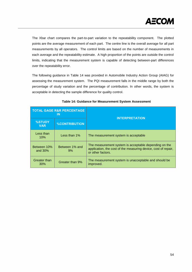
54
The Xbar chart compares the part-to-part variation to the repeatability component. The plotted
points are the average measurement of each part. The centre line is the overall average for all part
measurements by all operators. The control limits are based on the number of measurements in
each average and the repeatability estimate. A high proportion of the points are outside the control
limits, indicating that the measurement system is capable of detecting between-part differences
over the repeatability error.
The following guidance in Table 14 was provided in Automobile Industry Action Group (AIAG) for
assessing the measurement system. The PQI measurement falls in the middle range by both the
percentage of study variation and the percentage of contribution. In other words, the system is
acceptable in detecting the sample difference for quality control.
Table 14: Guidance for Measurement System Assessment
TOTAL GAGE R&R PERCENTAGE IN
INTERPRETATION
%STUDY VAR
%CONTRIBUTION
Less than 10%
Less than 1% The measurement system is acceptable
Between 10% and 30%
Between 1% and 9%
The measurement system is acceptable depending on the application, the cost of the measuring device, cost of repair, or other factors.
Greater than 30%
Greater than 9% The measurement system is unacceptable and should be improved.
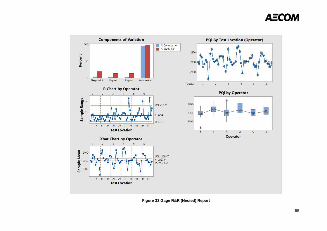
55
Figure 33 Gage R&R (Nested) Report
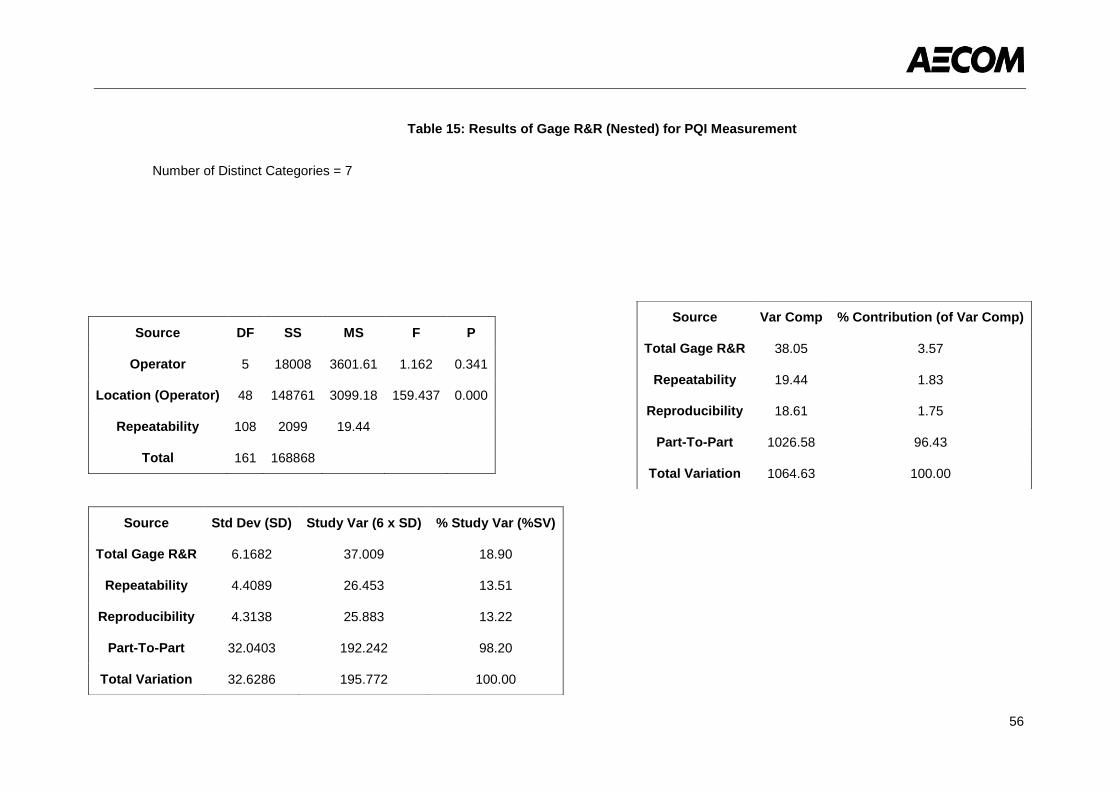
56
Table 15: Results of Gage R&R (Nested) for PQI Measurement
Number of Distinct Categories = 7
Source Var Comp % Contribution (of Var Comp)
Total Gage R&R 38.05 3.57
Repeatability 19.44 1.83
Reproducibility 18.61 1.75
Part-To-Part 1026.58 96.43
Total Variation 1064.63 100.00
Source Std Dev (SD) Study Var (6 x SD) % Study Var (%SV)
Total Gage R&R 6.1682 37.009 18.90
Repeatability 4.4089 26.453 13.51
Reproducibility 4.3138 25.883 13.22
Part-To-Part 32.0403 192.242 98.20
Total Variation 32.6286 195.772 100.00
Source DF SS MS F P
Operator 5 18008 3601.61 1.162 0.341
Location (Operator) 48 148761 3099.18 159.437 0.000
Repeatability 108 2099 19.44
Total 161 168868
57
7. CONCLUSIONS AND RECOMMENDATIONS
7.1. CONCLUSIONS
The objective of the research was to review and evaluate the available methods of measuring the
density of hot mix asphalt (HMA) pavements, specifically thin layers.
A comparison was undertaken between conventional coring bulk density methods (Destructive)
with methods such as Nuclear Density Gauge (NDG), electromagnetic, GPR, Step frequency radar
and indirect (non-destructive) compaction monitoring systems. Advantages and dis-advantages
were addressed based on literature reviewed. It was determined that trialling more mature methods
would provide a more industry ready/usable conclusion, particularly as there was difficulty sourcing
certain models and equipment within the UK.
For laboratory testing the Nuclear Density Gauge and Pavement Quality Indicator were compared
with each other and against the conventional coring method. The trials were designed to identify
accuracy whilst determining moisture and thickness susceptibility. A local contractor constructed
the asphalt trial at AECOM Nottingham Test Pit Facility (TPF), with various lift thicknesses and
degrees of compaction.
The precisions of both PQI and NDG readings are highly sensitive to the on-site calibration.
Detailed guidance on the calibration process is required for the use of NDG and PQI. It is
recommended to take regular calibration and to calibrate using a good spread of core densities,
e.g. 4% as suggested in BS 594987. Although BS 594987 recommends calibration using core
densities for all indirect density gauges, the mean of NDG Dry was closer to the mean core density
without this calibration. This may suggest the NDG pre-calibration using standard blocks is a
sound calibration method on its own. However, this is to be justified in further investigations.
The core density is the only direct measurement of the density and is used as the calibration
reference. Hence it is not included in the comparison.
A linear regression model was applied to examine the influential factors in the PQI and NDG
measurement systems. Thickness appears to be a statistically significant factor for PQI but not for
NDG. Although the manufacturer claims the moisture and temperature have been taken into
account in the built-in algorithm in PQI, moisture represented by H2O index and Dry/Wet condition
was predicted to be an influential factor in determining the PQI readings, so was temperature.
NDG also showed variable readings in the surface wet condition. Therefore, it is prudent to take
density measurements when the surface is dry using either PQI or NDG.
Romero (2000) suggested the moisture condition of H2O < 5 for reliable PQI readings. However it
was difficult to achieve even on a dry surface. The minimum H2O index in the surface dry
condition was 8.5. It is found that when H2O ≤ 12, all the measured densities are within ±5% of the
58
core densities. As the moisture level increased, the PQI measurements were more likely to deviate
from the corresponding core densities.
Comparing the measured air voids and the laboratory air voids, it is noted only 2% of NDG Dry
readings are less than the laboratory air voids, compared to 25% of PQI Dry. Testing under the
surface wet condition tends to introduce higher number of false readings for both NDG and PQI.
PQI and NDG are considered inadequate for quality assurance testing due to the wide spread of
data and sensitivity to calibration. But they are tenable for quality control testing. PQI is considered
acceptable in detecting the sample difference for quality control.
7.2. RECCOMENDATIONS
Indirect density measurements are subject to calibration and moisture condition. Current
equipment available to the market is not adequate for QA but acceptable for QC. To improve the
precision of indirect density gauges there should be:
A sound method for calibration.
The ability to consider moisture effect, and record/report details.
To be considered for QA acceptance, only if ±5% variation from core densities can be
demonstrated.
Later versions of the NDG and PQI may have increased precision, however, they are not currently
available in the UK for testing.
59
8. REFERENCES
AASHTO T-166 “Bulk Specific Gravity of Compacted Asphalt Mixtures Using Saturated Surface-
Dry Specimens”
AASHTO T 343-12 “Standard Method of Test for Density of In-Place Hot Mix Asphalt (HMA)
Pavement by Electronic Surface Contact Devices”
AASHTO TP 69 “Standard Method of Test for Bulk Specific Gravity and Density of Compacted
Asphalt Mixtures Using Automatic Vacuum Sealing Method”
ASTM Committee D04.21 (2009) “Interlaboratory Study to Establish Precision Statements for
ASTM D2950-09, Density of Bituminous Concrete in Place by Nuclear Methods”, Research Report
D04-1032, ASTM International
ASTM Committee D04.21 (2009) “Interlaboratory Study to Establish Precision Statements for
ASTM D7113-09, Standard Test Method for Density of Bituminous Paving Mixtures in Place by the
Electromagnetic Surface Contact Methods”, Research Report D04-1033, ASTM International
ASTM E691-15 “Standard Practice for Conducting an Internlaboratory Study to Determine the
Precision of a Test Method”, ASTM International
ASTM D2950/D2950M -14 “Standard Test Method for Density of Bituminous Concrete in Place by
Nuclear Methods”, ASTM International
ASTM D7113/D7113M – 10 “Standard Test Method for Density of Bituminous Paving Mixtures in
Place by the Electromagnetic Surface Contact Methods”, ASTM International
Allen, D. L., Schultz, D. B. and Willett, D. A. (2003) “Evaluation of Non-Nuclear Density Gauges”,
Report KTC-03-24/FR115-01-1F, Kentucky Transportation Centre, University of Kentucky
Al-Qadi, I. L. (1992) “Using Microwave Measurements to Detect Moisture in Asphaltic Concrete”
Journal of Testing and Evaluation, 20 (1), pp43-50
Al-Qadi, I. L., Leng Z. and Larkin A. (2011) “In-Place Hot Mix Asphalt Density Estimation Using
Ground Penetrating Radar”, ICT Report No. 11-096, University of Illinois, Federation Aviation
Administration
ASTM standard D7113 “Standard Test Method for Density of Bituminous Paving Mixtures in Place
by the Electomagnetic Surface Contact Methods”
Brown, E. R. (1990) “Density of Asphalt Concrete – How Much is Needed?”, NCAT Report No. 90-
3, 69th Annual Meeting of Transportation Researh Board, Washington, DC
60
Burati, J. L. and Elzoghbi, G. B. (1987) “Correlation of Nuclear Density Results with Core
Densities”, Transportation Research Board Record No. 1126, Transportation Research Board,
National Research council
BS 4987-2: 1988 Coated Macadam for Roads and Other Paved Areas Part 2 Specification for
Transport, Laying and Compaction, British Standards Institution
BS 594987: 2007 (updated in 2015) Asphalt for Roads and Other Paved Areas – Specification for
Transport, Laying, Compaction and Product-Type Testing Protocols, British Standards Institution
BS EN 12697-6: 2012 Bituminous Mixtures – Test Methods for Hot Mix Asphalt Part 6:
Determination of Bulk Density of Bituminous Specimens, British Standards Institution
BS EN 12697-8: 2003 Bituminous Mixtures – Test Methods for Hot Mix Asphalt – Part 8:
Determination of Void Characteristic of Bituminous Specimens, British Standards Institution
BS EN 12697-9: 2002 Bituminous Mixtures – Test Methods for Hot Mix Asphalt – Part 9:
Determination of the Reference Density, British Standards Institution
Choubane, B., Musselman, J. A., Page, G. C., Scholar, G. A. and Upshaw, P. B. (1999) “Nuclear
Density Readings and Core Densities – A Comparative Study”, Transportation Research Board
Record No. 1654, Transportation Research Board, National Research Council
"Compton, n.". OED Online. March 2016. Oxford University Press.
http://www.oed.com/view/Entry/37927?redirectedFrom=Compton+Effect (accessed April 18, 2016).
Commuri, S., Mai, Anh T., and Zaman, M. (2011) “Neural Network-Based Intelligent Compaction
Analyzer for Estimating Compaction Quality of Hot Asphalt Mixes”, ASCE Journal of Construction
Engineering and Management, doi:10.1061/(ASCE)CO.1943-7862.0000343
Dunning, M. R., Karakouzian, M. and Dunning, R. L. (2007) “Feasibility for the Use of Non-Contact
Ultrasound for Application in Asphalt Concrete Materials”, Journal of the Association of Asphalt
Paving Technologists, Vol. 76: 851-886,
Fauchard, C., Beaucamp B. and Laguerre L. (2015) “Non-Destructive Assessment of Hot Mix
Asphalt Compaction/ Density with a Step-Frequency Radar: Case Study on a Newly Paved Road”,
Glagola, C. R. (2003) “Pavement Quality Indicator: Investigator’s Summary”, Nomination 2003-02,
Construction Innovation Forum, University of Florida, Gainsville. FL.
Hunter, R.N. (2000) “Asphalts in Road Construction”, Thomas Telford Publishing, 1st Edition,
pp310-311
61
Highways Agency (2008) “Road Pavements – Bituminous Bound Materials”, Manual of Contract
Documents for Highway Works Volume 1 Specification for Highway Works Series 900, TSO,
London
Highways Agency (2008) “Series NG 900 Road Pavements – Bituminous Bound Materials”,
Manual of Contract Documents for Highway Works Volume 2 Notes for Guidance on the
Specification for Highway Works, TSO, London
Health and safety Executive (2002) “Portable nuclear moisture/density gauges in the construction
industry” HSE information sheet - Ionising Radiation Information Sheet No 3, Suffolk
Kassem, E., Scullion, T., Masad, E., Chowdhury, A., Liu, W., Estakhri, C. and Dessouky, S. (2012)
“Comprehensive Evaluation of Compaction of Asphalt Pavements and Development of Compaction
Monitoring System”, Report 0-6992-2, Texas Transportation Institute, Texas
Leng, Z. (2011) “Prediction of In-Situ Asphalt Mixture Density Using Ground Penetrating Radar:
Theoretical Development and Field Verification”, PhD Thesis, University of Illinois at Urbana-
Champaign
Lytton, R. L. (1995) “System Identification and Analysis of Subsurface Radar Signals”, US Patent
No. 5384715, Texas A&M University, Licensed to Lyric Technologies, Inc., Houston, TX.
Mason, M. E. (2008) “Investigation of Electromagnetic Gauges for Determination of In-Place
Density of HMA Pavements”, Master Thesis, Iowa State University, Iowa
Maupin, G. W. (2007) “Preliminary Field Investigation of Intelligent Compaction of Hot-Mix Asphal”,
Report No. VTRC 08-R7, Virginia Transportation Research Council, Charlottesville, VA.
Mitchell, T.D. (1984) “Density Monitoring on Asphalt Pavement”, Better Roads, Vol. 54, Issue 12,
pp.22-25
NCHRP IDEA projects 32 and 47, 1999
New Surface Geophysics, European Association of Geoscientists and Engineers (EAGE), 13 (3),
pp. 289-297 <10.3997/1873-0604.2015009>. <hal-01212038>
Padlo, P.T., Mahoney J., L., Aultman-Hall, L. and Zinke, S. (2005) “Correlation of Nuclear Density
Readings with Cores Cut from Compacted Roadways”, Report Number CT-2242-F-05-5. Storrs,
CT: Connecticut Transportation Institute, University of Connecticut
62
PaveTracker. PaveTracker Model 2701-B Plus. Website:
[http://www.troxlerlabs.com/Portals/0/Troxler%20Documents/Marketing%20Documents/PaveTrack
er%202701-B/2701BSS102015.pdf]. Accessed on 26/02/2016
Pellinen, T., Huuskonen-Snicker, E., Eskelinen, P. and Martinez P. O. (2015) “Representative
Volume Element of Asphalt Pavement for Electromagnetic Measurements”, Journal of Traffic and
Transportation Engineering, 2 (1): 30-39
Romeo, P. (2000) “Laboratory Evaluation of the PQI Model 300”, Final Draft Report for Multiple-
State Pooled Fund Study DTFH61-00-P-00549, Salt Lake City, UT: Department of Civil and
Environmental Engineering, University of Utah
Romeo, P. (2002) “Evaluation of Non-Nuclear Gauges to Measure Density of Hot-Mix Asphalt
Pavements”, Final Report for Multiple-State Pooled Fund Study DTFH61-00-P-00549, Salt Lake
City, UT: Department of Civil and Environmental Engineering, University of Utah
Sargand, S. M., Kim, S. and Farrington, S. P. (2005) “Non-Nuclear Density Gauge Comparative
Study”, Report No. FHWA/OH-2005, Ohio University
Sebesta, S. and Scullion, T. (2007) “Infrared Imaging and Ground – Penetrating Radar as Quality
Assurance Tools for Hot Mix Paving in Texas”, Asphalt Paving Technology: Association of Asphalt
Paving Technologists – Proceedings of the Technical Sessions 76, pp1-39
Stephens, J. (1964) “Evaluation of Nuclear and other Device Methods for Obtaining Bituminous
Paving Densities”, 6th Annual Paving Conference, Chicago, IL: Connecticut Bituminous Concrete
Producers Association
Solaimanian, M., Holmgreen, R. J. and Kennedy, T. W. (1990) “Evaluation of the Troxler Model
4640 Thin Lift Nuclear Density Gauge”, Research Report 468-1, Centre for Transportation
Research, University of Texas at Austin
Transport and Road Research Laboratory (1982) “Nuclear Gauges for Measuring the Density of
Roadbase Macadam Report of a Working Party”, Supplementary Report 754, ISSN 0305-1315,
Crowthorne, Berkshire
TransTech Systems. (2000) “Pavement Quality Indicator™ Model 300 Operator’s Handbook”, Rev
1, [http://www.transtechsys.com/pdf/PQIManual041000.pdf]
TransTech Systems. (2003) “Pavement Quality IndicatorTM Model 301 Operator’s Handbook”,
[http://www.transtechsys.com/pdf/PQI%20301%20Ophand.pdf]
63
TransTech Systems. (2016) “PQI 380 On-the-Run (OTR) Non-Nuclear Roller Mounted Asphalt
Density”, [http://www.transtechsys.com/products/otr.php], Accessed on 21/04/2016
Troxler Electronic Laboratories (2007) “Application Brief Troxler Model 3440 Roadreader Nuclear
Moisture Density Gauge”, Revision 2,
[http://www.troxlerlabs.com/downloads/pdfs/3440/3440appbrief.pdf]
Troxler Electronic Laboratories (2007) “Application Brief Troxler Model 3450, 3451 & 4640 Thin
Layer Nuclear Density Gauge Technology”,
[http://www.troxlerlabs.com/downloads/pdfs/4640/4640appbrief.pdf]
Troxler Electronic Laboratories (2013) “Application Brief Troxler Model 2701B PaveTracker™ Plus
Electromagnetic Sensing Device for Asphalt Quality Control”, Revision 5,
[https://www.troxlerlabs.com/downloads/pdfs/2701B/2701B_applicationbrief.pdf]
VicRoads (2011) “Technical Note 106 Surveillance of Field Density Testing by Nuclear Density
Gauge”, Victoria State Government, Australia
Volvo Construction Equipment (2015) “Density Direct – Volvo Intelligent Compaction”
[http://media.cygnus.com/files/base/FCP/document/2015/03/Volvo_IC_with_Density_Direct_Flyer_
0315.pdf] Accessed on 21/04/2016
Williams, R.C., Ceylan, H., Kvasnak, A.N. and Gopalakrishnan, K. (2007) Investigation of
Electromagnetic Gauges for Determining In-Place HMA Density. IHRB Project TR-547. Ames IA.
Centre for Transportation Research and Education, IOWA State University
Ziari, H., Izadi, B.A. and Divandary, H. (2010) Field Evaluation of Nondestructive Tests in
Measuring the Pavement Layers Density. Journal of Applied Sciences. 10 (23): 3091-3097e
Offset Slope
Recommended


![VARIOMATIC 2 + Asphalt-Manager Compaction.pdfSlide 14 Compaction of 6 cm asphalt binder course 0/10, ... vs. Marshall density [%] Compaction test on asphalt wearing course ... is of](https://img.pdfslide.us/doc/110x75/5abeef3e7f8b9a3a428d95f2/variomatic-2-asphalt-compactionpdfslide-14-compaction-of-6-cm-asphalt-binder.jpg)