Improvement of the Simulation of Cloud Longwave Scattering in BroadbandRadiative Transfer Models
GUANGLIN TANG,a PING YANG,a GEORGE W. KATTAWAR,b,c XIANGLEI HUANG,d ELI J. MLAWER,e
BRYAN A. BAUM,f AND MICHAEL D. KINGg,a
aDepartment of Atmospheric Sciences, Texas A&M University, College Station, TexasbDepartment of Physics and Astronomy, Texas A&M University, College Station, Texas
c Institute for Quantum Science and Engineering, Texas A&M University, College Station, TexasdDepartment of Climate and Space Sciences and Engineering, University of Michigan, Ann Arbor, Michigan
eAtmospheric and Environmental Research, Inc., Cambridge, Massachusettsf Space Science and Engineering Center, University of Wisconsin–Madison, Madison, Wisconsin
gLaboratory for Atmospheric and Space Physics, University of Colorado Boulder, Boulder, Colorado
(Manuscript received 11 January 2018, in final form 25 March 2018)
ABSTRACT
Cloud longwave scattering is generally neglected in general circulation models (GCMs), but it plays a
significant and highly uncertain role in the atmospheric energy budget as demonstrated in recent studies. To
reduce the errors caused by neglecting cloud longwave scattering, two new radiance adjustment methods are
developed that retain the computational efficiency of broadband radiative transfer simulations. In particular,
two existing scaling methods and the two new adjustment methods are implemented in the Rapid Radiative
Transfer Model (RRTM). The results are then compared with those based on the Discrete Ordinate Radi-
ative Transfer model (DISORT) that explicitly accounts for multiple scattering by clouds. The two scaling
methods are shown to improve the accuracy of radiative transfer simulations for optically thin clouds but not
effectively for optically thick clouds. However, the adjustment methods reduce computational errors over a
wide range, from optically thin to thick clouds. With the adjustment methods, the errors resulting from
neglecting cloud longwave scattering are reduced to less than 2Wm22 for the upward irradiance at the top of
the atmosphere and less than 0.5Wm22 for the surface downward irradiance. The adjustment schemes prove
to be more accurate and efficient than a four-stream approximation that explicitly accounts for multiple
scattering. The neglect of cloud longwave scattering results in an underestimate of the surface downward
irradiance (cooling effect), but the errors are almost eliminated by the adjustment methods (warming effect).
1. Introduction
It is commonly assumed that cloud longwave scatter-
ing is unimportant for estimating the atmospheric en-
ergy budget and thus is neglected in general circulation
model (GCM) irradiance simulations and in radiative
transfer simulations for deriving the radiation budgets
from retrieved cloud optical properties. A number of
studies indicate a range of overestimates of top-of-the-
atmosphere (TOA) longwave irradiance resulting from
neglecting longwave scattering. For example, Stephens
et al. (2001) showed an overestimation of global-average
outgoing longwave radiation (OLR) of approximately
8Wm22 when cloud longwave scattering is neglected
in a GCM, whereas regional overestimation could be as
large as 20Wm22. Costa and Shine (2006) showed
a global overestimation of OLR of approximately
3Wm22 by neglecting cloud longwave scattering, with
low-level clouds contributing 0.9Wm22, midlevel
clouds contributing 0.7Wm22, and high clouds con-
tributing 1.4Wm22. Other studies also reported OLR
overestimations resulting from neglecting cloud long-
wave scattering with values ranging from 1.5 to 11Wm22
(Ritter and Geleyn 1992; Joseph and Min 2003; Schmidt
et al. 2006). In a recent sensitivity study, Kuo et al. (2017)
showed that neglecting cloud longwave scattering could
result in an overestimation of the global-average OLR
of approximately 2.6Wm22 and an overestimation of
the surface net upward radiation of approximately
1.1Wm22.
Such significant changes caused by excluding cloud
longwave scattering effects suggest a pressing need forCorresponding author: Guanglin Tang, [email protected]
JULY 2018 TANG ET AL . 2217
DOI: 10.1175/JAS-D-18-0014.1
� 2018 American Meteorological Society. For information regarding reuse of this content and general copyright information, consult the AMS CopyrightPolicy (www.ametsoc.org/PUBSReuseLicenses).
more accurate longwave radiative transfer (RT) simula-
tions in the broadband radiance models used in GCMs.
However, such a change should not substantially increase
the computational burden, since the computational costs
of the RT models in GCMs are already high. One ap-
proach for mitigating the computational burden is to scale
the cloud absorption optical thickness, as in the scheme
developed by Chou et al. (1999). The Chou et al. scheme
retains the computational efficiency by neglecting the
longwave scattering and improves accuracy for irradiance
in the case of optically thin clouds. However, there is little
improvement for optically thick clouds, as the TOA
longwave irradiance is still overestimated by approxi-
mately 4Wm22. Therefore, simply scaling the cloud
optical thickness in conjunction with no-scattering simula-
tions is insufficient for further improvement of irradiance
calculations over a range of optical thicknesses.
The similarity principle for radiative transfer (van de
Hulst 1974; Sobolev 1975; Joseph et al. 1976; van de
Hulst 1980; Twomey and Bohren 1980; McKellar and
Box 1981; Ding et al. 2017) provides an alternative ap-
proach for scaling the optical thickness. The basic con-
cept is that radiance or irradiance simulations may have
similar results with two different sets of cloud optical
properties if the optical properties satisfy certain re-
lationships. With this principle, one could consider
replacing a scattering cloud layer with a nearly non-
scattering cloud layer and obtain similar irradiance
values. The similarity principle has been verified for
TOA solar radiance calculations (with an external
source and a nonemitting atmosphere) with a single-
scattering albedov between 0.8 and 1 and an asymmetry
factor g between 0.75 and 0.9 (Ding et al. 2017). How-
ever, further investigation is necessary for the case of
small v (i.e., strongly absorptive case) and for longwave
irradiance from a scattering–emitting cloud layer where
there is no external source term. As with the Chou et al.
scheme, a simple scaling strategy also lacks the ability to
provide accurate irradiance calculations for optically
thick clouds. These two schemes are compared in this
study (section 3) and have similar results for the irradi-
ance simulations.
The primary goal of this study is to develop a new
adjustment scheme based on the similarity principle
and the Chou scaling schemes. We will show that this
adjustment scheme improves the longwave irradiance
calculations in a broadband radiative transfer model
for both optically thin and thick ice clouds. Although
the present scheme also works for low-level liquid
water clouds, we will not show results for this case
because the scattering effect is generally weak in the
longwave regime.
The remaining part of the paper is organized as fol-
lows: Section 2 discusses the methodology. Section 3
presents the simulation results and discussions. Section 4
summarizes and concludes the study.
2. Methodology
a. Similarity principle
Previous derivations of the similarity relation fo-
cused on a nonemitting atmosphere (McKellar and
Box 1981; van de Hulst 1974; King 1981; Ding et al.
2017) that can be extended to an emitting atmosphere
straightforwardly following the derivation of Ding
et al. (2017). For longwave scattering without exter-
nal sources, the radiance is independent of azimuth.
The azimuthally averaged radiative transfer equation
(RTE) for a plane-parallel atmosphere, following Liou
[1980, Eq. (6.1.12)], is
m›I(t,m)
›t5 I(t,m)2 [12v(t)]B(t)
2v(t)
2
ð121
I(t,m0)P(m,m0) dm0 , (1)
where I is the radiance, m and m0 indicate the cosines of
the angles between the propagating direction of I and
the zenith (positive for upward radiance and negative
for downward radiance), t is the optical thickness (zero
at TOA and positive at the surface), B is the blackbody
radiance (Planck function of temperature and wave-
length), andP(m,m0) is the azimuthally averaged scattering
phase function. The dependence of Eq. (1) on wave-
length is implied. By multiplying Eq. (1) with the
lth-order Legendre polynomial pl(m), followed by in-
tegrating over m, the result is
ð121
m›I(t,m)
›tpl(m) dm5
ð121
I(t,m)pl(m) dm2 [12v(t)]B(t)d
0l2
v(t)
2
ð121
ð121
I(t,m0)P(m,m0)pl(m) dm0 dm , (2)
where d0l is the Kronecker delta function. Expansion
of P(m,m0) in terms of Legendre polynomials and
application of the addition theorem (Edmonds 2016;
Wiscombe 1977) yields
2218 JOURNAL OF THE ATMOSPHER IC SC IENCES VOLUME 75

P(m,m0)5 �‘
l50
(2l1 1)xlpl(m)p
l(m0) , (3)
where xl is the lth coefficient of the Legendre expansion
of the phase function. By noting the orthogonality of
Legendre polynomials, we substitute Eq. (3) into Eq. (2)
to obtain
ð121
�m›I(t,m)
›t2 I(t,m)[12v(t)x
l]
�pl(m) dm
52[12v(t)]B(t)d0l. (4)
From Eq. (4), obtaining an invariant I(t, m) with a dif-
ferent set of optical properties requires that
t0(12v0x0l)5 t(12vx
l), l5 0, 1, 2, . . .‘ , (5)
which is true because the thermal emission term van-
ishes for all l other than zero. Variables with or without
primes indicate two different sets of optical properties.
This similarity relation is the same as for a nonemitting
atmosphere (McKellar and Box 1981). Normally, it is
impossible to satisfy Eq. (5) for all l except when two sets
of optical properties are exactly the same. However, we
may consider the first two lowest-order values for l to
obtain approximate similarity relations. Specifically, l 5 0
and l5 1 (x0 5 1 and x1 5 g) result in the following two
similarity relations, respectively, which involve three
important variables, t, v, and g:
t0(12v0)5 t(12v) , (6a)
t0(12v0g0)5 t(12vg) . (6b)
If t0, v0, and g0 are considered as unknowns, then Eq. (6)
has 1 degree of freedom. Setting g0 5 0 (isotropic scat-
tering) results in
t0 5 t(12vg), v0 5v(12 g)
(12vg). (7)
For an isotropic scattering layer that has been used to
perform the two-stream approximation for the long-
wave radiative transfer in the GCM Model I (Hansen
1969; Hansen et al. 1983), this is relatively accurate for a
single layer but the accuracy degrades for multiple
layers combined using the adding method.
In contrast, keeping only the first-order l5 0 results in
Eq. (6a), which still has a single degree of freedom.
Setting v0 5 0 yields
t0 5 t(12v), v0 5 0, (8)
which implies no scattering. In other words, neglect-
ing the scattering with t0 5 t(1 2 v) corresponds to
assuming that all scattering is solely in the forward di-
rection (i.e., g 5 1), which can be interpreted as direct
transmission. The reason the TOA irradiance is over-
estimated is because the side- and backscattering of the
upward radiance is accounted for as being directly
transmitted to TOA.
To mitigate the aforesaid flaw, one could consider
scaling (increasing) the absorption optical thickness
to compensate for the overestimated upward transmis-
sion. However, with v0 5 0, Eq. (6) has no solution. We
choose a t0 value so that the square error of Eq. (6) is
minimized under the condition of v0 5 0:
t0 5 t
�12v
11 g
2
�, v0 5 0. (9)
The difference between this scaled optical thickness
t0 5 t[1 2 v(1 1 g)/2] and the absorbing optical thick-
ness t0 5 t(12v) is the term tv(12 g)/2, which is half of
what is identified as the scattering optical thickness ac-
cording to Twomey and Bohren (1980). Qualitatively,
because t[1 2 v(1 1 g)/2] is larger than t(1 2 v), we
expect a reduction of the overestimation of TOA irradi-
ance.However, such a simple optical thickness scalingmay
not be sufficient for optically thick clouds. Thus, multiple
scattering needs to be treated in a more rigorous way.
b. Chou’s parameterization for adjusting the cloudoptical thickness
In addition to the similarity principle scaling scheme,
another scheme for adjusting the cloud optical thickness
was developed by Chou et al. (1999) and is briefly
summarized as follows. We approximate the upward
and downward radiance with two respective constants.
For example, the Chou et al. (1999) approach approxi-
mates the radiance in the integration term in Eq. (1) in
the form
I(t,m0)’�I(t,m), m3m0 . 0
B(t), m3m0 , 0. (10)
In this way, the ambient radiance I(t, m0) in the integral
term in the RTE Eq. (1) is assumed to be isotropic in
each of the upward and downward hemispheres. It
equals the incident radiance I(t, m) when they are in the
same hemisphere and equals the ambient blackbody
radiance when they are in different hemispheres. For
example, when solving the downward radiance, all
downward radiance terms in Eq. (1) are assumed to be a
single unknown, while all upward radiance terms are
approximated in terms of the Planck radiation. Hence,
the downward and upward radiances are decoupled in
Eq. (1). The integration source term in Eq. (1) can be
expressed as
JULY 2018 TANG ET AL . 2219
ð121
I(t,m0)P(m,m0) dm0 ’
8>>>>>>><>>>>>>>:
I(t,m)
ð021
P(m,m0) dm0 1B(t)
ð10
P(m,m0) dm0, m, 0
I(t,m)
ð10
P(m,m0) dm0 1B(t)
ð021
P(m,m0) dm0, m. 0
. (11)
The termsÐ 10P(m, m0) dm0 and
Ð 021
P(m, m0) dm0 are func-
tionsofm, but theycanbeapproximatedby theiraveragesover
m so as to be constants; note that the sumof these two terms is
2 because they are normalized. Then Eq. (11) is rewritten as
ð121
I(t,m0)P(m,m0) dm0 ’�I(t,m)3 (22 2b)1B(t)3 2b, m, 0I(t,m)3 (22 2b)1B(t)3 2b, m. 0
, (12)
where
b[1
2
ð10
dm
ð021
P(m,m0) dm0 [1
2
ð021
dm
ð10
P(m,m0) dm0
’ 12 �4
i51
aigi21 , (13)
with a1 5 0.5, a2 5 0.3738, a3 5 0.0076, and a4 5 0.1186
(Chou et al. 1999). Note that the phase function P(m, m0)is approximated in terms of the Henyey–Greenstein
function—that is, a function of only g, m, and m0—and
is fitted with a fourth-order polynomial. Substituting
Eq. (12) into Eq. (1) yields
m›I(t,m)
[12v(12b)]›t5 I(t,m)2B(t) . (14)
Because v is assumed to be constant in each layer in
radiative transfer models (RTMs), the role of the factor
1 2 v(1 2 b) in Eq. (14) is simply to scale the optical
thickness and to represent the radiative transfer equa-
tion in a nonscattering form.
With the similarity principle approach, replacing
1 2 b with (1 1 g)/2 in Eq. (14) leads to a similar radi-
ative transfer equation:
m›I(t,m)
12v(11 g)
2
� �›t
5 I(t,m)2B(t) . (15)
The only difference between the similarity principle
scaling scheme and Chou’s scaling scheme is the scaling
factor 1 2 v(1 1 g)/2 versus [1 2 v(1 2 b)]. Note that
when g5 1 orv5 0, both schemes reduce to the original
scheme that neglects scattering:
m›I(t,m)
(12v)›t5 I(t,m)2B(t) . (16)
c. Adjustment scheme
In the Chou et al. (1999) scaling scheme, the major
approximation is with the hemispheric isotropic radi-
ance. The performance of the scheme highly depends on
the extent to which this approximation holds true.While
one can consider the ambient radiance as being ap-
proximately equal to the incident radiance in the same
hemisphere, large biases may result from this approxi-
mation when the incident radiance is in the opposite
hemisphere, especially for downward ambient radiance
on top of a cloud layer. In this case, the downward am-
bient radiance is much weaker than the blackbody ra-
diance. Hence, we reconsider the approximation for the
downward ambient radiance when solving for the up-
ward radiance.
When neglecting scattering, RTMs first solve for the
downward radiance, layer by layer from the TOA to the
surface, and then the upward radiance from the surface
to the TOA. The governing equation [Eq. (16)] is a first-
order ordinary differential equation with a boundary
condition that the downward radiance at TOA is zero. In
such a process, when solving for the upward radiance,
the downward radiance is already known. This means
that the ambient downward radiance is not necessarily
assumed to be the blackbody radiance when solving for
the upward radiance. Equation (12) then becomes
ð121
I(t,m0)P(m,m0) dm0 ’�I(t,m)3 (22 2b)1B(t)3 2b, m, 0I(t,m)3 (22 2b)1 I(t,2m)3 2b, m. 0
. (17)
2220 JOURNAL OF THE ATMOSPHER IC SC IENCES VOLUME 75

Note that the term I(t, 2m) in the upward direction
(m . 0) is obtained by solving for the downward
direction first. Substitution of Eq. (17) into Eq. (1)
yields
m›I(t,m)
[12v(12 b)]›t5 I(t,m)2B(t), m, 0: (18a)
m›I(t,m)
[12v(12 b)]›t5 I(t,m)2B(t)2
vb
12v(12b)[I(t,2m)2B(t)], m. 0: (18b)
Note the additional term2vb/[12v(12 b)]3 [I(t,2m)2B(t)] in Eq. (18b), which is the only difference between
the new scheme and the Chou et al. scheme. We use
Eq. (18a) to solve for the downward radiance from the
TOA to the surface, and then substitute the resulting
downward radiance into Eq. (18b) to solve for the up-
ward radiance from the surface to the TOA. The process
proceeds layer by layer. A specific solution is necessary
for solving the upward radiance at the (n 1 1)th level
from the nth level, which satisfies
m›Iss(t,m)
[12v(12 b)]›t5 Iss(t,m)2
vb
12v(12 b)[I(t,2m)2B(t)], m. 0, (19)
with a boundary condition of Iss(tn, m) 5 0. Here Iss de-
notes the specific solution for the nth layer t 2 [tn11, tn],
and tn, n5 0, 1, . . . ,N is the optical depth at the top of the
nth layer (n5 0 is for the surface and n5 N is for TOA).
For simplicity, we assume B to be constant within a layer,
which is reasonable when the temperature varies little within
a layer. Then, fromEq. (18a) we know that I(t,2m)2 B(t)
changes exponentially with t and is given by
I(t,2m)2B(t)5 [I(tn11
,2m)2B(tn11
)] exp
�2[12v(12 b)](t2 t
n11)
m
�, for m. 0, t
n11, t, t
n. (20)
Note that B is assumed constant in this process. Sub-
stitution of Eq. (20) into Eq. (19) results in a first-
order ordinary differential equation involving Iss(t, m).
Furthermore, I(tn11, 2m) is known from the previous
process for solving for the downward radiances. The
solution for the differential equation leads to
Iss(tnþ1
,m) ¼ vb
2[12v(12 b)]
0@[I(t
nþ1,2m)2B(t
nþ1)]2 [I(t
n,2m)2B(t
n)]
3 exp
8<:2
[12v(12 b)](tn2 t
nþ1)
m
9=;1A, for m. 0, (21)
where the exponential term exp{2[1 2 v(1 2 b)]
(tn 2 tn11)/m} is the transmissivity of the nth layer after
scaling.We call this specific solution the adjustment term,
and it is determined from the known downward radi-
ance. To be more accurate, B can be assumed to be a
linear function of t, for example, in the RRTM (Mlawer
et al. 1997; Iacono et al. 2000). However, as long as the
temperature does not change significantly within a layer,
the exponential solution for the downward radiance
given in Eq. (20) is still a reasonable approximation.
Hence, the final solution of the upward radiance at the
(n1 1)th level is the general solution to the nonscattering
radiative equation [Eq. (14)] plus the specific upward ra-
diance adjustment given by Eq. (21). We call the scheme
with this solution the Chou scaling-adjustment scheme.
The specific solution is basically negative, leading to a
JULY 2018 TANG ET AL . 2221

reduction of the overestimates of the upward irradiance,
especially above high clouds. In particular, when the
layer is very thin, in Eq. (21) I(tn11, 2m) 2 B(tn11) is
similar to I(tn, 2m) 2 B(tn) and the transmissivity term
exp{2[1 2 v(1 2 b)](tn 2 tn11)/m} approaches unity and
therefore the adjustment term is very small.When the layer
is optically thick and high, exp{2[1 2 v(1 2 b)](tn 2tn11)/m} and I(tn11, 2m) approach zero and therefore
the adjustment term approaches2vb/2[12v(12 b)]3B(tn11), a negative value. Also, the adjustment in-
creases with cloud optical thickness, which is ideal for
mitigating the weakness of the two scaling schemes for
optically thick clouds.
Alternatively, the term (1 2 b) may be replaced with
(11 g)/2 in Eqs. (14) and (21) to obtain general and specific
solutions based on the similarity principle. We call the
scheme with this solution the similarity scaling-adjustment
scheme. In Chou’s scheme, (1 2 b) represents the per-
centage of the scattering contribution in the direction of
the to-be-solved radiance from the ambient radiance in
the same hemisphere, and b represents the contribution
from the ambient radiance in the opposite hemisphere.
In the similarity scaling-adjustment scheme, with (11 g)/2
replacing (1 2 b), the percentage contributions from the
ambient radiance in the two hemispheres are (1 1 g)/2
and (1 2 g)/2, respectively. When g 5 1, the scattering
contribution to the to-be-solved radiance is purely from
the ambient radiance in the same hemisphere. When g50, the contributions from the two hemispheres are equal,
corresponding to isotropic scattering. The appendix de-
scribes the physical meaning of the similarity principle
scaling and the adjustment term. In a simplified model
where the atmosphere is a one-dimensional, optically thin
layer, the similarity principle scaling scheme results in
more accurate TOA irradiance than the neglect-scattering
scheme, and the similarity scaling-adjustment schemeresults
in the exact solution, completely offsetting the error of the
scaling scheme.
After solving for the upward radiance, the downward
radiance can be adjusted by using the known upward
radiance following an equation similar to Eq. (21) but
from the TOA to the surface:
Iss(tn21
,m) ¼ vb
2[12v(12 b)]
�[I(t
n21,2m)2B(t
n21)]2 [I(t
n,2m)2B(t
n)]
3 exp
�2
[12v(12 b)](tn21
2 tn)
2m
��, for m, 0, (22)
where n 5 1, 2, . . .,N is the nth level, and then the
solved downward radiance can change the upward
radiance solution again. This iterative process may
lead to a considerable increase of computational time.
Alternatively, we can optimize the scale of the ad-
justment term given by Eq. (21) to minimize the error
for a number of simulations and use only ‘‘one and a
half’’ iterative steps. Based on the simulations, the
coefficient 0.5 (or 1/2) in Eq. (21) can be replaced by
values of 0.4 and 0.3 for the similarity and the Chou
scaling-adjustment schemes, respectively. This coeffi-
cient optimization is partly because of several as-
sumptions we have made. In summary, the first step of
this approach is to solve for the downward radiance
without adjustment and then to solve for the upward
radiance with adjustment given by Eq. (21) with opti-
mized coefficients. Eventually, the downward radiance
is adjusted by the term given by Eq. (22) with the same
optimized coefficient. The computational time is al-
most the same as the original scheme that neglects
longwave scattering. All schemes used in this study
along with their corresponding governing equations
(and specific solution) and approximate computa-
tional time are listed in Table 1.
3. Results
Wepresent results for the four schemes discussed in the
previous section: the Chou et al. scaling approach, the
similarity principle scaling approach, the Chou scaling-
adjustment scheme, and the similarity scaling-adjustment
scheme. For evaluation purposes, we implement all four
schemes in the RRTM longwave model, a simplified ver-
sion [RRTM for General Circulation Models (RRTMG)]
of which has been used to simulate radiative transfer in
multiple GCMs, such as the Community Earth System
Model (CESM;Kay et al. 2015) and theWeatherResearch
and Forecasting (WRF)Model (Powers et al. 2017). In the
RRTM longwave model, the upward and downward
radiances are calculated for a set of radiance spectral
bands, without considering scattering, for a single or
multiple (1–4) angles, and then integrated to provide
the irradiance. Cloud scattering can also be included
using the DISORT option in RRTM, but it is much
slower computationally.
For the purpose of generality, we use multiple ice
cloud particle models to represent the ice cloud optical
properties. In addition to the built-in spherical ice
particle model (Hu and Stamnes 1993; Key 1996;
2222 JOURNAL OF THE ATMOSPHER IC SC IENCES VOLUME 75
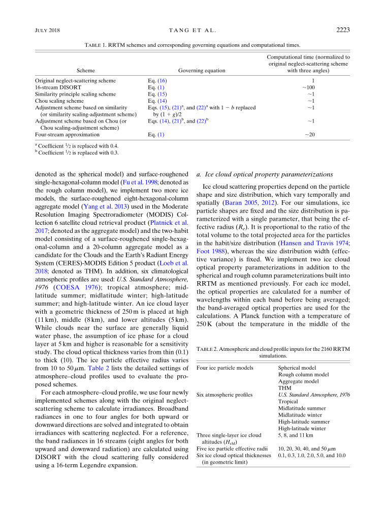
denoted as the spherical model) and surface-roughened
single-hexagonal-columnmodel (Fu et al. 1998; denoted as
the rough column model), we implement two more ice
models, the surface-roughened eight-hexagonal-column
aggregate model (Yang et al. 2013) used in the Moderate
Resolution Imaging Spectroradiometer (MODIS) Col-
lection 6 satellite cloud retrieval product (Platnick et al.
2017; denoted as the aggregatemodel) and the two-habit
model consisting of a surface-roughened single-hexag-
onal-column and a 20-column aggregate model as a
candidate for the Clouds and the Earth’s Radiant Energy
System (CERES)-MODIS Edition 5 product (Loeb et al.
2018; denoted as THM). In addition, six climatological
atmospheric profiles are used: U.S. Standard Atmosphere,
1976 (COESA 1976); tropical atmosphere; mid-
latitude summer; midlatitude winter; high-latitude
summer; and high-latitude winter. An ice cloud layer
with a geometric thickness of 250m is placed at high
(11 km), middle (8 km), and lower altitudes (5 km).
While clouds near the surface are generally liquid
water phase, the assumption of ice phase for a cloud
layer at 5 km and higher is reasonable for a sensitivity
study. The cloud optical thickness varies from thin (0.1)
to thick (10). The ice particle effective radius varies
from 10 to 50mm. Table 2 lists the detailed settings of
atmosphere–cloud profiles used to evaluate the pro-
posed schemes.
For each atmosphere–cloud profile, we use four newly
implemented schemes along with the original neglect-
scattering scheme to calculate irradiances. Broadband
radiances in one to four angles for both upward or
downward directions are solved and integrated to obtain
irradiances with scattering neglected. For a reference,
the band radiances in 16 streams (eight angles for both
upward and downward radiation) are calculated using
DISORT with the cloud scattering fully considered
using a 16-term Legendre expansion.
a. Ice cloud optical property parameterizations
Ice cloud scattering properties depend on the particle
shape and size distribution, which vary temporally and
spatially (Baran 2005, 2012). For our simulations, ice
particle shapes are fixed and the size distribution is pa-
rameterized with a single parameter, that being the ef-
fective radius (Re). It is proportional to the ratio of the
total volume to the total projected area for the particles
in the habit/size distribution (Hansen and Travis 1974;
Foot 1988), whereas the size distribution width (effec-
tive variance) is fixed. We implement two ice cloud
optical property parameterizations in addition to the
spherical and rough column parameterizations built into
RRTM as mentioned previously. For each ice model,
the optical properties are calculated for a number of
wavelengths within each band before being averaged;
the band-averaged optical properties are used for the
calculations. A Planck function with a temperature of
250K (about the temperature in the middle of the
TABLE 2.Atmospheric and cloud profile inputs for the 2160RRTM
simulations.
Four ice particle models Spherical model
Rough column model
Aggregate model
THM
Six atmospheric profiles U.S. Standard Atmosphere, 1976
Tropical
Midlatitude summer
Midlatitude winter
High-latitude summer
High-latitude winter
Three single-layer ice cloud
altitudes (Hcld)
5, 8, and 11 km
Five ice particle effective radii 10, 20, 30, 40, and 50mm
Six ice cloud optical thicknesses
(in geometric limit)
0.1, 0.3, 1.0, 2.0, 5.0, and 10.0
TABLE 1. RRTM schemes and corresponding governing equations and computational times.
Scheme Governing equation
Computational time (normalized to
original neglect-scattering scheme
with three angles)
Original neglect-scattering scheme Eq. (16) 1
16-stream DISORT Eq. (1) ;100
Similarity principle scaling scheme Eq. (15) ;1
Chou scaling scheme Eq. (14) ;1
Adjustment scheme based on similarity
(or similarity scaling-adjustment scheme)
Eqs. (15), (21)a, and (22)a with 1 2 b replaced
by (1 1 g)/2
;1
Adjustment scheme based on Chou (or
Chou scaling-adjustment scheme)
Eqs. (14), (21)b, and (22)b ;1
Four-stream approximation Eq. (1) ;20
a Coefficient 1/2 is replaced with 0.4.b Coefficient 1/2 is replaced with 0.3.
JULY 2018 TANG ET AL . 2223

troposphere) is used as the weighting function for av-
eraging. The size distribution is a gamma function with
an effective variance fixed to be 0.1, consistent with that
used in the MODIS Collection 6 and CERES-MODIS
retrieval products.
Figure 1 shows the scattering property parameteriza-
tions of four ice particle models for two effective radii,
10 and 30mm, as functions of the RRTM bands. Note
that smaller particles have larger v and smaller g, both
of which lead to stronger scattering effects. For the at-
mospheric window bands (about 700–1200 cm21), v is
about 0.4–0.7 and g is about 0.9. This means ice clouds
scatter nearly as much thermal radiation as they absorb.
Because the gas absorption in the window bands is weak,
ice cloud scattering plays a more important role in the
radiative transfer than in other bands. The difference
between the four ice models is roughly 0.1 for v and 0.03
for g. In particular, the rough column model tends to
have the largest v and smallest g and thus has the
strongest scattering effect. The aggregate model has
moderate v and the largest g. Natural ice cloud particles
have even more complicated geometries than the four
icemodels presented (Baran 2009). However, we use the
four ice particle models to represent the natural vari-
ability of particle geometries and to test the perfor-
mance of the newly developed schemes without losing
too much generality.
b. RRTM simulations
We implement the four schemes discussed in section 2
into the standard RRTM release (version 3.3): the Chou
scaling approach, the similarity principle scaling ap-
proach, the Chou scaling-adjustment scheme, and the
similarity scaling-adjustment scheme. In addition, there
are two schemes available in RRTM: one neglects
scattering and the other uses DISORT to more accu-
rately solve the radiative transfer equation.
For each of the 2160 atmosphere–cloud profiles,
we performed irradiance calculations with these six
schemes. The DISORT calculations are performed with
16 streams and a 16-order Legendre expansion, the re-
sults of which serve as a reference for the error estima-
tion of the other five schemes. The DISORT calculation
was compared to the rigorous line-by-line DISORT
FIG. 1. Scattering property parameterizations of four ice particle models for RRTM, which divides the longwave
spectral region (10–3250 cm21) into 16 bands for radiation calculations (vertical dashed lines). Columns are for
Re 5 (left) 10 and (right) 30mm. Rows are (top) single-scattering albedo and (bottom) asymmetry factor.
2224 JOURNAL OF THE ATMOSPHER IC SC IENCES VOLUME 75
(Turner et al. 2003; Turner 2005) benchmark and was
within 2Wm22 in terms of TOA irradiance. (We com-
pared RRTM 16-stream simulations with the line-by-
line DISORT counterparts with a 0.01-cm21 spectral
resolution for 540 of the atmosphere–cloud profiles in
Table 2 with the ice particle chosen to be the aggregate
model.) The surface emissivity is assumed to be unity (no
reflection), which is reasonable for calculations over ocean
and snow, since their emissivity is very close to 1 (about
0.97–0.99) at around 11mm (Masuda et al. 1988; Li et al.
2013), the central wavelength of the thermal infrared re-
gime, though all of the schemes are able to deal with a
nonunity surface albedo by adding the reflection of the
surface downward irradiance and the surface emission to
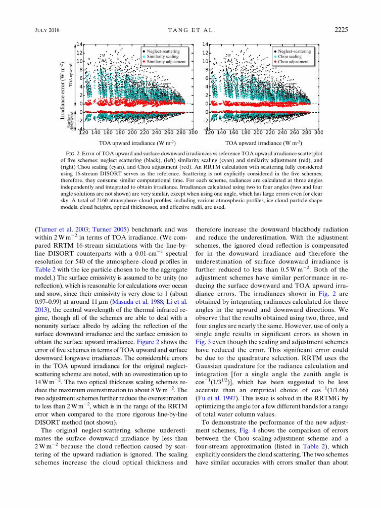
obtain the surface upward irradiance. Figure 2 shows the
error of five schemes in terms of TOA upward and surface
downward longwave irradiances. The considerable errors
in the TOA upward irradiance for the original neglect-
scattering scheme are noted, with an overestimation up to
14Wm22. The two optical thickness scaling schemes re-
duce the maximum overestimation to about 8Wm22. The
two adjustment schemes further reduce the overestimation
to less than 2Wm22, which is in the range of the RRTM
error when compared to the more rigorous line-by-line
DISORT method (not shown).
The original neglect-scattering scheme underesti-
mates the surface downward irradiance by less than
2Wm22 because the cloud reflection caused by scat-
tering of the upward radiation is ignored. The scaling
schemes increase the cloud optical thickness and
therefore increase the downward blackbody radiation
and reduce the underestimation. With the adjustment
schemes, the ignored cloud reflection is compensated
for in the downward irradiance and therefore the
underestimation of surface downward irradiance is
further reduced to less than 0.5Wm22. Both of the
adjustment schemes have similar performance in re-
ducing the surface downward and TOA upward irra-
diance errors. The irradiances shown in Fig. 2 are
obtained by integrating radiances calculated for three
angles in the upward and downward directions. We
observe that the results obtained using two, three, and
four angles are nearly the same. However, use of only a
single angle results in significant errors as shown in
Fig. 3 even though the scaling and adjustment schemes
have reduced the error. This significant error could
be due to the quadrature selection. RRTM uses the
Gaussian quadrature for the radiance calculation and
integration [for a single angle the zenith angle is
cos21(1/31/2)], which has been suggested to be less
accurate than an empirical choice of cos21(1/1.66)
(Fu et al. 1997). This issue is solved in the RRTMG by
optimizing the angle for a few different bands for a range
of total water column values.
To demonstrate the performance of the new adjust-
ment schemes, Fig. 4 shows the comparison of errors
between the Chou scaling-adjustment scheme and a
four-stream approximation (listed in Table 2), which
explicitly considers the cloud scattering. The two schemes
have similar accuracies with errors smaller than about
FIG. 2. Error of TOAupward and surface downward irradiances vs reference TOAupward irradiance scatterplot
of five schemes: neglect scattering (black), (left) similarity scaling (cyan) and similarity adjustment (red), and
(right) Chou scaling (cyan), and Chou adjustment (red). An RRTM calculation with scattering fully considered
using 16-stream DISORT serves as the reference. Scattering is not explicitly considered in the five schemes;
therefore, they consume similar computational time. For each scheme, radiances are calculated at three angles
independently and integrated to obtain irradiance. Irradiances calculated using two to four angles (two and four
angle solutions are not shown) are very similar, except when using one angle, which has large errors even for clear
sky. A total of 2160 atmosphere–cloud profiles, including various atmospheric profiles, ice cloud particle shape
models, cloud heights, optical thicknesses, and effective radii, are used.
JULY 2018 TANG ET AL . 2225

1Wm22 in terms of TOA upward irradiance, but the
four-stream approximation is demonstrably worse for
optically thin clouds. The four-stream approximation
consumes a computational time of about 20 times that
of the adjustment scheme. Therefore, the adjustment
schemes have both better accuracy and computational
efficiency than the four-stream approximation.
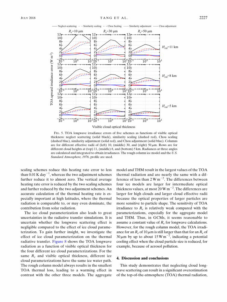
Figure 5 shows the TOA upward irradiance error as a
function of visible optical thickness for different values
of the cloud height and cloud effective radius. The
original neglect-scattering scheme always overestimates
the TOA upward irradiance and is at a maximum for
intermediate optical thickness (;1), which is consistent
with Kuo et al. (2017). Qualitatively, the scattering is
less effective for optically thin clouds, while for optically
thick clouds the effect of scattering is partly offset by
the absorption. The overestimation decreases with Re
because the impact of scattering decreases with Re as
a result of v increasing and g decreasing with Re in
the atmospheric window spectral region. The over-
estimation increases with cloud height because the
upward irradiance resulting from scattering in a higher
cloud layer is less affected by the atmosphere above the
cloud. The two scaling schemes reduce the overestimation
significantly for small and intermediate optical thicknesses
but approach the neglect-scattering scheme for large optical
thicknesses. In fact, the no-scattering simulations always
approach a constant value for large optical thickness. The
two adjustment schemes further reduce the overestimation
to less than 2Wm22 over the entire range of optical
thicknesses.
Figure 6 is similar to Fig. 5, but it shows the error of
surface downward irradiance as a function of visible op-
tical thickness. The original neglect-scattering scheme
underestimates the surface downward irradiance and
similarly has a maximum value for intermediate optical
thickness. The error also decreases with Re but decreases
with height, because the cloud reflection of upward ra-
diation is less affected by the atmosphere beneath the
clouds. The two scaling schemes again reduce the error
significantly for thin and intermediate optical thicknesses
but approach the results from the neglect-scattering
scheme for high optical thicknesses. Both of the ad-
justment schemes reduce the errors for all optical
thickness values to less than 0.5Wm22.
Figure 7 shows the vertical distribution of the heating
rate error for each of the five schemes for an intermediate
(;1) cloudoptical thickness. The original neglect-scattering
scheme basically underestimates the heating rate beneath
cloud by about 0.1K day21, indicating a cooling effect on
the atmosphere, consistent with the overestimation of
the TOA upward irradiance. The cloud scattering
plays a role in reflecting upward thermal radiance and
warming the atmosphere below the cloud. The two
FIG. 4. Comparison of TOA upward irradiance error between
the adjustment scheme based on Chou’s scaling scheme (cyan) and
a four-stream approximation (red).
FIG. 3. As in Fig. 2, but with the radiance calculated for one zenith angle for both upward and downward radiation.
2226 JOURNAL OF THE ATMOSPHER IC SC IENCES VOLUME 75
scaling schemes reduce this heating rate error to less
than 0.01K day21, whereas the two adjustment schemes
further reduce it to almost zero. The vertical average
heating rate error is reduced by the two scaling schemes
and further reduced by the two adjustment schemes. An
accurate calculation of the thermal heating rate is es-
pecially important at high latitudes, where the thermal
radiation is comparable to, or may even dominate, the
contribution from solar radiation.
The ice cloud parameterization also leads to great
uncertainties in the radiative transfer simulations. It is
uncertain whether the longwave scattering effect is
negligible compared to the effect of ice cloud parame-
terization. To gain further insight, we investigate the
effect of ice cloud parameterization on the thermal
radiative transfer. Figure 8 shows the TOA longwave
radiation as a function of visible optical thickness for
the four different ice cloud parameterizations. For the
same Re and visible optical thickness, different ice
cloud parameterizations have the same ice water path.
The rough column model always results in the smallest
TOA thermal loss, leading to a warming effect in
contrast with the other three models. The aggregate
model and THM result in the largest values of the TOA
thermal radiation and are nearly the same with a dif-
ference of less than 2Wm22. The differences between
four ice models are larger for intermediate optical
thickness values, at most 20Wm22. The differences are
larger for high clouds and larger cloud effective radii
because the optical properties of larger particles are
more sensitive to particle shape. The sensitivity of TOA
irradiance to Re is relatively weak compared with the
parameterizations, especially for the aggregate model
and THM. Thus, in GCMs, it seems reasonable to
assume a constant value of Re for longwave calculations.
However, for the rough column model, the TOA irradi-
ance for anRe of 10mm is still larger than that for anRe of
30mm by up to about 15Wm22, indicating a potential
cooling effect when the cloud particle size is reduced, for
example, because of aerosol pollution.
4. Discussion and conclusions
This study demonstrates that neglecting cloud long-
wave scattering can result in a significant overestimation
of the top-of-the-atmosphere (TOA) thermal radiation,
FIG. 5. TOA longwave irradiance errors of five schemes as functions of visible optical
thickness: neglect scattering (solid black), similarity scaling (dashed red), Chou scaling
(dashed blue), similarity adjustment (solid red), and Chou adjustment (solid blue). Columns
are for different effective radii of (left) 10, (middle) 30, and (right) 50mm. Rows are for
different cloud heights at (top) 11, (middle) 8, and (bottom) 5 km. Radiances at three angles
are calculated and integrated to obtain irradiances. The rough column ice model and theU.S.
Standard Atmosphere, 1976, profile are used.
JULY 2018 TANG ET AL . 2227

which in turn leads to a spurious cooling effect below the
clouds. The overestimation can be as large as 14Wm22
depending on the cloud thickness, altitude, and optical
properties. In general, the overestimation reaches its
highest values for a higher cloud of an intermediate
optical thickness with relatively small cloud particles.
Additionally, neglecting cloud longwave scattering
leads to an underestimate in the surface downward
FIG. 6. As in Fig. 5, but for the surface downward irradiance error.
FIG. 7. As in Fig. 5, but for heating rate error of the five schemes as a function of height. The
cloud optical thickness is 1.
2228 JOURNAL OF THE ATMOSPHER IC SC IENCES VOLUME 75

irradiance—or in other words, it overestimates the sur-
face net upward irradiance by up to 2Wm22. Neglecting
multiple scattering in lower clouds results in larger er-
rors in the surface downward irradiance.
Theoretically, clouds scatter longwave upward ra-
diation to the side and backward directions and
therefore reduce the thermal radiation reaching the
TOA while also increasing the thermal radiation re-
flected back to surface. Thus, neglecting scattering
overestimates TOA thermal radiation and underes-
timates surface downward radiation. By increasing
the cloud absorptive optical thickness while still
neglecting scattering, less thermal radiation reaches
the TOA and more blackbody radiation emanating
from clouds reaches the surface, and thus both TOA
and surface radiation errors are reduced. However,
for optically thick clouds, increasing the cloud ab-
sorptive optical thickness offers little improvement
because the irradiance changes little with increasing
optical thickness. We applied the similarity principle
and Chou et al.’s (1999) scaling schemes to RRTM
and verified the conclusion stated above. For optically
thick clouds, the TOA irradiance overestimation can
still reach 8Wm22.
We developed adjustment schemes for both the sim-
ilarity principle and Chou et al. (1999) scaling schemes,
in which the downward radiances are calculated and
then used to adjust the upward radiances. In an itera-
tive process, the upward radiances are again used to
adjust the downward radiances. A negative adjustment
term for the upward radiance is derived that increases
with cloud optical thickness and approaches a constant
for very thick clouds. The adjustment term for the
downward radiance is similar but positive. In such a
way, the TOA and surface irradiance errors are further
reduced. We applied these two schemes to RRTM
and found that the TOA upward and surface down-
ward irradiance errors are reduced to less than 2 and
0.5Wm22, respectively, over a wide range of optical
thickness values. The comparison with the four-stream
approximation shows that the new adjustment schemes
are more accurate than the four-stream approximation
and about 20 times faster computationally.
The simulations are performed for various atmo-
spheric profiles, cloud heights, optical thicknesses, ice
particle sizes, and cloud optical property parameteriza-
tions. As a reference to evaluate the error, the cloud
scattering is considered with a 16-stream DISORT
computation in RRTM, which has been shown to agree
with rigorous line-by-line DISORT benchmarks within
2Wm22 for all sky conditions.
In addition, considering that the similarity principle
failed to improve the two-stream approximation for mul-
tiple layers combined with the adding method, we further
FIG. 8. As in Fig. 5, but for TOA longwave irradiance as a function of visible cloud optical
thickness for four different ice cloud models: spherical (dark blue), rough column (green),
aggregate (red), and THM (light blue). RRTM with 16-stream DISORT is used in the
simulations.
JULY 2018 TANG ET AL . 2229

verified the new schemes for multiple cloud layers and
obtained very similar errors as for single layers (not
shown). We conclude that the adjustment schemes are
effective in improving the accuracy of longwave radiative
transfer for virtually all sky conditions.
In the RRTM simulations, we found that the radiance
computed at a single Gaussian quadrature angle is in-
sufficient for the irradiance integral, similar to the study
by Fu et al. (1997). More than one Gaussian quadrature
angle results in relatively accurate irradiance integrals.
Thus, we suggest using at least two Gaussian quadrature
angles to solve the longwave radiative transfer equation
in a broadband radiative transfer model such as RRTM.
Cloud longwave scattering has a warming effect be-
neath clouds of up to 0.1K day21, but this is neglected in
most GCMs. The scaling and adjustment schemes help
to account for such a warming effect.
We also found that the broadband irradiances are
sensitive to the ice cloud optical property parameteri-
zation. The differences between different parameteri-
zations are of similar magnitude to the scattering effect
itself. As studies involving the remote sensing of clouds
are leading to more accurate cloud microphysics pa-
rameterizations, the new schemes, in conjunction with
more realistic cloudmicrophysical illustrations, will help
improve the energy budget estimation.
Finally, we note that RRTMG, as a GCM version of
RRTM, uses one angle following Fu et al. (1997) with
optimizations in a few bands as a function of the total
column water. Further improvement of the RRTMG by
using more than one angle and the adjustment schemes
will be explored in future work.
Acknowledgments. This study was supported by the
National Science Foundation (AGS-1632209) and partly
by the endowment funds related to the David Bullock
Harris Chair in Geosciences at the College of Geo-
sciences, Texas A&MUniversity. The effort of coauthor
Huang is supported by the U.S. Department of Energy,
Office of Science, Office of Biological and Environ-
mental Research, Climate and Environmental Science
Division under Award DE-SC0012969 to the University
of Michigan. The simulations are conducted through the
Texas A&M supercomputing facility.
APPENDIX
Physical Meaning of the Similarity Scaling andAdjustment
To understand the physical meaning of the similarity
principle and the adjustment term, we simplify the at-
mosphere to be a single cloudy layer with a uniform
temperature of Tc, an optical thickness of tc, a single-
scattering albedo ofv, and an asymmetry factor of g. We
further assume that the radiation is one-dimensional,
meaning that we can think of this as a representation of
upward and downward irradiances, so then we can use
an exact solution of the irradiance (Kattawar and Plass
1973). The surface temperature and emissivity are
assumed to be TS and unity, respectively. This sim-
plified model approximately describes the behavior of
the radiative transfer in the atmosphere and is used to
understand the similarity principle and the adjustment
term. We consider the single-scattering scenario,
where tc � 1. In this case, the cloud layer absorbs a
fraction of (1 2 v) of the total extinction of the up-
ward irradiance from the surface, and scatters a frac-
tion of v[(11 g)/2] upward and a fraction of v[(12 g)/2]
back downward to the surface. Then the TOA upward
irradiance is
F[(0)5 e2tcpBS1 (12 e2tc)v
11 g
2pB
S
1 (12 e2tc)(12v)pBc, (A1)
where F[ is the upward irradiance as a function of t, with
F[(0) being the TOA irradiance. The quantities BS and
Bc are the blackbody radiance for temperatures TS and Tc,
respectively. The quantities pBS and pBc are thus the
blackbody irradiances of the surface and the cloud layer,
respectively. The three terms on the right-hand side of
Eq. (A1) are the transmitted surface irradiance to the
TOA, scattered surface irradiance at the TOA, and at-
mospheric thermal irradiance at the TOA, respectively.
For an optically thin layer (tc � 1), e2tc ’ 1 2 tc, and
Eq. (A1) is simplified as
F[(0)5 (12 tc)pB
S1 t
cv11 g
2pB
S1 t
c(12v)pB
c
5
�12
�12v
11 g
2
�tc
�pB
S1 (12v)t
cpB
c.
(A2)
Now we consider neglecting the scattering by replacing
tc and v with tc(1 2 v) and zero, respectively, and
removing the scattering term in Eq. (A2). Then the
solution is
F[(0)5 [12 (12v)tc]pB
S1 01 t
c(12v)pB
c
5 [12 (12v)tc]pB
S1 (12v)t
cpB
c. (A3)
Simply setting g to be 1 in Eq. (A2) also results in Eq.
(A3). From the exact solution [Eq. (A2)] to the neglect-
scattering solution Eq. (A3), the transmitted surface
blackbody radiative irradiance to the TOA increases
2230 JOURNAL OF THE ATMOSPHER IC SC IENCES VOLUME 75
by vtcpBS because the optical thickness decreases; the
upward scattered irradiancedecreases by tcv[(11 g)/2]pBS
to zero because the scattering is neglected; and the at-
mospheric emission to TOA remains unchanged because
the absorptive optical thickness does not change. In sum,
the neglect-scattering solution is tcv[(12 g)/2]pBc larger
than the exact solution.
Further, we consider the similarity principle scaling
solution by replacing tc and v with tc[1 2 v(1 1 g)/2]
and zero, respectively, and removing the scattering term
in Eq. (A2). Then the solution is
F[(0)5
�12
�12v
11 g
2
�tc
�pB
S1 01 t
c
�12v
11 g
2
�pB
c5
�12
�12v
11 g
2
�tc
�pB
S1
�12v
11 g
2
�tcpB
c.
(A4)
From the exact solution [Eq. (A2)] to the similarity principle
scaling solution [Eq. (A4)], the transmitted surface black-
body irradiance to TOA increases byv[(11 g)/2]tcpBS; the
upward scattered irradiance decreases by tcv[(11 g)/2]pBS
to zero to offset the transmission increase; and the atmo-
spheric emission to TOA increases by tcv[(1 2 g)/2]pBc
Taken together, the similarity principle scaling solution is
tcv[(1 2 g)/2]pBc larger than the exact solution.
The error of the similarity principle scaling solution
tcv[(1 2 g)/2]pBc is basically smaller than that of the
neglect-scattering solution tcv[(1 2 g)/2]pBS because
the cloud temperature is lower than the surface tem-
perature, especially when the cloud layer is high. The error
of the similarity scaling scheme comes from the increase of
the cloud thermal radiation resulting from larger absorptive
optical thickness.
Moreover, we consider an adjustment term ap-
plied to the similarity principle scaling solution,
which according to Eq. (21) is [replacing (12 b) with
(1 1 g)/2]
F[ss(0)5v12 g
2
2 12v11 g
2
� ��[FY(0)2pB
c]2 [FY(t
c)2pB
c] exp
�2
�12v
11 g
2
�tc
��
5v12 g
2
2 12v11 g
2
� ��2pB
c2
�12v
11 g
2
�tcpB
c1pB
c
�12
�12v
11 g
2
�tc
��52v
12 g
2tcpB
c, (A5)
where F[ss is the specific solution of the upward irradi-
ance and also is a function of t. Note that the trans-
missivity of the cloud layer is exp{2[1 2 v(1 1 g)/2]tc}
and the relation
FY(0)5 0
FY(tc)5
�12v
11 g
2
�tcpB
c
(A6)
is used in the derivation of Eq. (A5). The errors of the
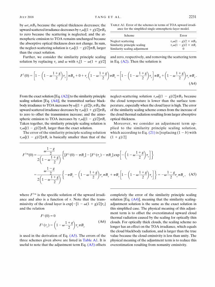
three schemes given above are listed in Table A1. It is
useful to note that the adjustment term Eq. (A5) offsets
completely the error of the similarity principle scaling
solution [Eq. (A4)], meaning that the similarity scaling-
adjustment solution is the same as the exact solution in
this simplified case. The physical meaning of this adjust-
ment term is to offset the overestimated upward cloud
thermal radiation caused by the scaling for optically thin
clouds. For optically thick clouds, the scaling scheme no
longer has an effect on the TOA irradiance, which equals
the cloud blackbody radiation, and is larger than the true
value because the cloud emissivity is less than unity. The
physical meaning of the adjustment term is to reduce this
overestimation resulting from nonunity emissivity.
TABLE A1. Error of the schemes in terms of TOA upward irradi-
ance for the simplified single-atmospheric-layer model.
Scheme Error
Neglect scattering tcv(1 2 g)/2 3 pBS
Similarity principle scaling tcv(1 2 g)/2 3 pBc
Similarity scaling adjustment 0
JULY 2018 TANG ET AL . 2231

REFERENCES
Baran, A. J., 2005: The dependence of cirrus infrared radiative
properties on ice crystal geometry and shape of the size dis-
tribution function.Quart. J. Roy.Meteor. Soc., 131, 1129–1142,
https://doi.org/10.1256/qj.04.91.
——, 2009: A review of the light scattering properties of cirrus.
J. Quant. Spectrosc. Radiat. Transfer, 110, 1239–1260, https://
doi.org/10.1016/j.jqsrt.2009.02.026.
——, 2012: From the single-scattering properties of ice crystals to
climate prediction: A way forward. Atmos. Res., 112, 45–69,
https://doi.org/10.1016/j.atmosres.2012.04.010.
Chou, M.-D., K.-T. Lee, S.-C. Tsay, and Q. Fu, 1999: Parame-
terization for cloud longwave scattering for use in atmo-
spheric models. J. Climate, 12, 159–169, https://doi.org/
10.1175/1520-0442-12.1.159.
COESA, 1976: U.S. Standard Atmosphere, 1976. NOAA, 227 pp.
Costa, S. M. S., and K. P. Shine, 2006: An estimate of the global
impact of multiple scattering by clouds on outgoing long-wave
radiation. Quart. J. Roy. Meteor. Soc., 132, 885–895, https://
doi.org/10.1256/qj.05.169.
Ding, J., P. Yang, G. W. Kattawar, M. D. King, S. Platnick, and
K. G. Meyer, 2017: Validation of quasi-invariant ice cloud
radiative quantities with MODIS satellite-based cloud prop-
erty retrievals. J. Quant. Spectrosc. Radiat. Transfer, 194,
47–57, https://doi.org/10.1016/j.jqsrt.2017.03.025.
Edmonds, A. R., 2016: Angular Momentum in Quantum Mechan-
ics. Princeton University Press, 160 pp.
Foot, J. S., 1988: Some observations of the optical properties of
clouds. II: Cirrus. Quart. J. Roy. Meteor. Soc., 114, 145–164,
https://doi.org/10.1002/qj.49711447908.
Fu, Q., K. N. Liou, M. C. Cribb, T. P. Charlock, and A. Grossman,
1997:Multiple scattering parameterization in thermal infrared
radiative transfer. J. Atmos. Sci., 54, 2799–2812, https://doi.
org/10.1175/1520-0469(1997)054,2799:MSPITI.2.0.CO;2.
——, P. Yang, and W. B. Sun, 1998: An accurate parameterization
of the infrared radiative properties of cirrus clouds for climate
models. J. Climate, 11, 2223–2237, https://doi.org/10.1175/
1520-0442(1998)011,2223:AAPOTI.2.0.CO;2.
Hansen, J. E., 1969: Absorption-line formation in a scattering plan-
etary atmosphere: A test of van de Hulst’s similarity relations.
Astrophys. J., 158, 337–349, https://doi.org/10.1086/150196.
——, and L. D. Travis, 1974: Light scattering in planetary atmo-
spheres. Space Sci. Rev., 16, 527–610, https://doi.org/10.1007/
BF00168069.
——, G. Russell, D. Rind, P. Stone, A. Lacis, S. Lebedeff,
R. Ruedy, and L. Travis, 1983: Efficient three-dimensional
global models for climate studies: Models I and II.Mon. Wea.
Rev., 111, 609–662, https://doi.org/10.1175/1520-0493(1983)
111,0609:ETDGMF.2.0.CO;2.
Hu, Y. X., and K. Stamnes, 1993: An accurate parameterization of
the radiative properties of water clouds suitable for use in
climate models. J. Climate, 6, 728–742, https://doi.org/10.1175/
1520-0442(1993)006,0728:AAPOTR.2.0.CO;2.
Iacono,M. J., E. J. Mlawer, S. A. Clough, and J.-J. Morcrette, 2000:
Impact of an improved longwave radiation model, RRTM, on
the energy budget and thermodynamic properties of the
NCAR community climate model, CCM3. J. Geophys. Res.,
105, 14 873–14 890, https://doi.org/10.1029/2000JD900091.
Joseph, E., and Q. Min, 2003: Assessment of multiple scattering
and horizontal inhomogeneity in IR radiative transfer calcu-
lations of observed thin cirrus clouds. J. Geophys. Res., 108,
4380, https://doi.org/10.1029/2002JD002831.
Joseph, J. H.,W. J.Wiscombe, and J. A.Weinman, 1976: The delta-
Eddington approximation for radiative flux transfer. J. Atmos.
Sci., 33, 2452–2459, https://doi.org/10.1175/1520-0469(1976)
033,2452:TDEAFR.2.0.CO;2.
Kattawar, G. W., and G. N. Plass, 1973: Interior radiances in op-
tically deep absorbing media—I. Exact solutions for one-
dimensional model. J. Quant. Spectrosc. Radiat. Transfer, 13,
1065–1080, https://doi.org/10.1016/0022-4073(73)90080-0.
Kay, J. E., and Coauthors, 2015: The Community Earth System
Model (CESM) large ensemble project: A community re-
source for studying climate change in the presence of internal
climate variability. Bull. Amer. Meteor. Soc., 96, 1333–1349,
https://doi.org/10.1175/BAMS-D-13-00255.1.
Key, J., 1996: Streamer user’s guide. Boston University Tech. Rep.
96-01, 85 pp.
King, M. D., 1981: A method for determining the single scattering
albedo of clouds through observation of the internal scattered
radiation field. J. Atmos. Sci., 38, 2031–2044, https://doi.org/
10.1175/1520-0469(1981)038,2031:AMFDTS.2.0.CO;2.
Kuo,C.-P., P. Yang, X.Huang,D. Feldman,M. Flanner, C. Kuo, and
E. J. Mlawer, 2017: Impact of multiple scattering on longwave
radiative transfer involving clouds. J. Adv.Model. Earth Syst., 9,
3082–3098, https://doi.org/10.1002/2017MS001117.
Li, Z.-L., H. Wu, N. Wang, S. Qiu, J. A. Sobrino, Z. Wan, B.-H.
Tang, and G. Yan, 2013: Land surface emissivity retrieval
from satellite data. Int. J. Remote Sens., 34, 3084–3127,
https://doi.org/10.1080/01431161.2012.716540.
Liou, K. N., 1980: An Introduction to Atmospheric Radiation.
Vol. 26. Academic Press, 391 pp.
Loeb, N.G., andCoauthors, 2018: Impact of ice cloudmicrophysics
on satellite cloud retrievals and broadband flux radiative
transfer model calculations. J. Climate, 31, 1851–1864, https://
doi.org/10.1175/JCLI-D-17-0426.1.
Masuda, K., T. Takashima, and Y. Takayama, 1988: Emissivity of
pure and sea waters for the model sea surface in the infrared
window regions. Remote Sens. Environ., 24, 313–329, https://
doi.org/10.1016/0034-4257(88)90032-6.
McKellar, B. H. J., and M. A. Box, 1981: The scaling group of the
radiative transfer equation. J. Atmos. Sci., 38, 1063–1068, https://
doi.org/10.1175/1520-0469(1981)038,1063:TSGOTR.2.0.CO;2.
Mlawer, E. J., S. J. Taubman, P. D. Brown, M. J. Iacono, and S. A.
Clough, 1997: Radiative transfer for inhomogeneous atmo-
spheres: RRTM, a validated correlated-k model for the
longwave. J. Geophys. Res., 102, 16 663–16 682, https://doi.org/
10.1029/97JD00237.
Platnick, S., and Coauthors, 2017: The MODIS cloud optical and
microphysical products: Collection 6 updates and examples
from Terra and Aqua. IEEE Trans. Geosci. Remote Sens., 55,
502–525, https://doi.org/10.1109/TGRS.2016.2610522.
Powers, J. G., and Coauthors, 2017: The Weather Research and
Forecasting (WRF) Model: Overview, system efforts, and fu-
ture directions. Bull. Amer. Meteor. Soc., 98, 1717–1737,
https://doi.org/10.1175/BAMS-D-15-00308.1.
Ritter, B., and J.-F. Geleyn, 1992: A comprehensive radiation scheme
for numerical weather prediction models with potential applica-
tions in climate simulations.Mon.Wea.Rev., 120, 303–325, https://
doi.org/10.1175/1520-0493(1992)120,0303:ACRSFN.2.0.CO;2.
Schmidt, G. A., and Coauthors, 2006: Present-day atmospheric
simulations using GISS ModelE: Comparison to in situ,
satellite, and reanalysis data. J. Climate, 19, 153–192, https://
doi.org/10.1175/JCLI3612.1.
Sobolev, V. V., 1975: Rasseianie sveta v atmosferakh planet (Light
Scattering in Planetary Atmospheres). Pergamon Press, 256 pp.
2232 JOURNAL OF THE ATMOSPHER IC SC IENCES VOLUME 75

Stephens, G. L., P. M. Gabriel, and P. T. Partain, 2001: Parame-
terization of atmospheric radiative transfer. Part I: Validity of
simple models. J. Atmos. Sci., 58, 3391–3409, https://doi.org/
10.1175/1520-0469(2001)058,3391:POARTP.2.0.CO;2.
Turner, D. D., 2005: Arctic mixed-phase cloud properties fromAERI
lidar observations: Algorithm and results from SHEBA. J. Appl.
Meteor., 44, 427–444, https://doi.org/10.1175/JAM2208.1.
——, S. A. Ackerman, B. A. Baum, H. E. Revercomb, and P. Yang,
2003: Cloud phase determination using ground-based AERI
observations at SHEBA. J. Appl. Meteor., 42, 701–715, https://
doi.org/10.1175/1520-0450(2003)042,0701:CPDUGA.2.0.CO;2.
Twomey, S., and C. F. Bohren, 1980: Simple approximations for calcu-
lations of absorption in clouds. J. Atmos. Sci., 37, 2086–2095, https://
doi.org/10.1175/1520-0469(1980)037,2086:SAFCOA.2.0.CO;2.
van de Hulst, H. C., 1974: The spherical albedo of a planet cov-
ered with a homogeneous cloud layer.Astron. Astrophys., 35,
209–214.
——, 1980: Multiple Light Scattering: Tables, Formulas, and Ap-
plications. Vol. 2, Academic Press, 436 pp.
Wiscombe, W. J., 1977: The delta–M method: Rapid yet accurate
radiative flux calculations for strongly asymmetric phase
functions. J. Atmos. Sci., 34, 1408–1422, https://doi.org/10.1175/1520-0469(1977)034,1408:TDMRYA.2.0.CO;2.
Yang, P., L. Bi, B. A. Baum, K.-N. Liou, G. W. Kattawar, M. I.
Mishchenko, and B. Cole, 2013: Spectrally consistent scatter-
ing, absorption, and polarization properties of atmospheric ice
crystals at wavelengths from 0.2 to 100mm. J. Atmos. Sci., 70,
330–347, https://doi.org/10.1175/JAS-D-12-039.1.
JULY 2018 TANG ET AL . 2233
Recommended