Import Protection as Export Destruction
Hiroyuki Kasahara∗ Beverly Lapham†
December 2005
Incomplete
Abstract
This paper develops a dynamic, stochastic industry model of heterogeneous firms to examine
the effects of trade liberalization on resource reallocation, industry productivity, and welfare
in the presence of import and export complementarities. The model highlights mechanisms
whereby import policies affect exports and export policies affect imports. We first present a
simplified version of the model and use that theoretical model to develop an empirical model
which we structurally estimate using Chilean plant-level manufacturing data. A comparison of
our estimates of transition probabilities across export/import status with the data suggests a
need for a dynamic approach. We then examine a dynamic version and structurally estimate
that model using the same data set. The estimated model is used to perform counterfactual
experiments regarding different trading regimes to assess the positive and normative effects of
barriers to trade in import and export markets. These experiments suggest that the welfare
gain due to trade is substantial and because of import and export complementarities, policies
which inhibit the importation of foreign intermediates can have a large adverse effect on the
exportation of final goods.
∗University of Western Ontario†Queen’s University; The author gratefully acknowledges financial support from the Social Sciences Humanities
Council of Canada.
1

1 Introduction
This paper develops a dynamic stochastic industry model of heterogeneous firms to examine the
effects of trade liberalization on resource reallocation, industry productivity, and welfare in the
presence of import and export complementarities. We use the theoretical model to develop an
empirical model which we estimate using Chilean plant-level manufacturing data. The estimated
model is then used to perform counterfactual experiments regarding different trading regimes
to assess the positive and normative effects of barriers to trade in import and export markets.
The theoretical trade literature with increasing returns typically identifies two effects on
productivity of firms as trade increases: the scale effect as surviving firms increase output and
produce at lower average cost and the selection effect as firms are forced to exit. As Melitz
(2003) has shown in a model with heterogeneous exporting firms, the least productive firms will
typically exit due to the selection effect. Thus resources will be reallocated to more productive
firms, and aggregate productivity will rise.
Indeed, empirical work suggests that there is a substantial amount of resource reallocation
across firms within an industry following trade liberalization and these shifts in resources do
contribute to productivity growth in the sector. Pavcnik (2002) uses Chilean data and finds
that such reallocations contribute to productivity growth after trade liberalization in that coun-
try. Trefler (2004) estimates these effects in Canadian manufacturing following the U.S.-Canada
free trade agreement using plant- and industry-level data and finds significant increases in pro-
ductivity among both importers and exporters. Empirical evidence also suggests that relatively
more productive firms are more likely to export (see, for example, Bernard and Jensen(1999),
Aw, Chung, and Roberts (2000), and Clerides, Lack and Tybout (1998)).
In this paper we provide empirical evidence that suggests that whether or not a firm is
importing intermediates for use in production may also be important for explaining differences
in plant performance (see also, Kasahara and Rodrigue 2004). Our data suggests that firms
which are both importing and exporting tend to be larger and more productive than firms that
are active in either market, but not both. Hence, the impact of trade on resource reallocation
across firms which are importing may be as important as shifts across exporting firms.
To simultaneously address the empirical regularities concerning importers, we begin by ex-
tending the model of Melitz (2003) to incorporate imported intermediate goods. In this environ-
2

ment, we allow final goods producers to differ with regard to both their productivity and their
fixed cost of importing. We also incorporate complementarities in the fixed costs of importing
and exporting. In the model, the use of foreign intermediates increases firm’s productivity but,
due to the presence of fixed costs of importing, only inherently high productive firms importing
intermediates. Trade liberalization which lowers restrictions on the importation of intermediates
increases aggregate productivity because some inherently productive firms start importing and
achieve within-plant productivity gains. This, in turn, leads to a resource reallocation from less
productive to more productive importing firms. Furthermore, productivity gains among highly
productive firms through imported intermediates may allow some of them to start exporting,
leading to a resource reallocation in addition to that emphasized by Melitz(2003). Similarly,
events that encourage exporting (e.g., liberalization in trading partners or export subsidies) may
well have an impact on firm’s decision to import since newly exporting firms would have a higher
incentive to start importing. Thus, the model identifies an important mechanism whereby import
tariff policy affects aggregate exports and whereby export subsidies affect aggregate imports.
To quantitatively examine the impact of trade on aggregate productivity and welfare, we es-
timate a stochastic industry equilibrium model of exports and imports using a panel of Chilean
manufacturing plants. Our estimates suggest significant complementarities in both sunk and
fixed costs of importing and exporting. Furthermore, the basic observed patterns of produc-
tivity across firms with different import and export status is well captured by the estimated
model. We also perform a variety of counterfactual experiments to examine the effects of trade
policies. The experiments suggest that the welfare gain due to exposure to trade is found to be
substantial. Another important finding is that because of import and export complementarities,
policies which inhibit the importation of foreign intermediates can have a large adverse effect on
the exportation of final goods. In addition, the experiments indicate that the equilibrium price
response plays a major role in redistributing resources from less productive firms to more pro-
ductive firms. In particular, experiments based on a partial equilibrium model that ignores the
equilibrium price response provide fairly different estimates of the impact of trade on aggregate
productivity.
Not surprisingly the static model is not well-suited to capture the observed transition prob-
abilities of plants across different import and export categories. With this in mind, we extend
the basic empirical model to incorporate dynamic elements and estimate this model with the
3

same data set. The fundamental insights gained from the static estimation continue to hold in
the dynamic model. In addition, we find evidence of dynamic complementarities in fixed costs
of importing and exporting. That is, a firm which is importing in the current period faces a cost
advantage to begin exporting in subsequent periods. We also demonstrate that the dynamic
model is broadly consistent with the transition probabilities across import and export status
categories.
The remainder of the paper is organized as follows. Section 2 presents empirical evidence
on the static and dynamic distribution of importers and exporters and their performance using
Chilean manufacturing plant-level data. Section 3 presents a theoretical model with import and
export complementarities. Section 4 presents a static empirical model based on the theoretical
model developed in the previous section. Section 5 discusses the data used and the results of
the structural estimation of the static model. Sections 6 and 7 present a dynamic extension of
the empirical model and the estimation methodology for the dynamic model. Section 8 presents
the dynamic empirical results and Section 9 concludes.
2 Empirical Motivation
In this section we briefly describe Chilean plant-level data and provide summary statistics to
characterize patterns and trends of plants which may or may not participate in international
markets.
2.1 Data
We use the Chilean manufacturing census for 1990-1996. In the data set, we observe the number
of blue collar workers and white collar workers, the value of total sales, the value of export sales,
and the value of imported materials. The export/import status of a firm is identified from the
data by checking if the value of export sales and/or the value of imported materials are zero
or positive. The value of the revenue from the home market is computed as (the value of total
sales)-(the value of export sales). We use the manufacturing output price deflator to convert
the nominal value into the real value. The entry/exiting decisions can be identified in the data
by looking at the number of workers across years. We use unbalanced panel data of 7234 plants
for 1990-1996, including all the plants that have been observed at least one year between 1990
4

Table 1: Exporters and Importers in Chile for 1990-1996 (% of Total)
1990 1991 1992 1993 1994 1995 1996 1990-96 ave.
Exporters 8.7 9.4 9.2 9.2 8.5 9.8 8.7 9.1
Importers 12.8 11.9 13.1 13.2 13.2 12.2 11.6 12.6
Ex/Importers 8.2 9.6 10.7 12.0 13.1 12.4 12.7 11.2
Exports by Exporters 43.1 42.9 49.3 42.5 34.0 39.3 39.3 41.5
Exports by Ex/Importers 56.9 57.1 50.7 57.5 66.0 60.7 60.7 58.5
Imports by Importers 35.2 31.7 31.5 28.7 21.2 22.0 25.4 28.0
Imports by Ex/Importers 64.8 68.3 68.5 71.3 78.8 78.0 74.6 72.0
Output by Exporters 17.9 16.3 23.4 19.0 15.1 20.3 17.6 18.5
Output by Importers 16.7 12.8 14.9 15.3 13.8 14.3 13.5 14.5
Output by Ex/Importers 38.8 44.5 40.5 44.1 50.1 45.4 48.3 44.5
No. of Plants 4722 4628 4938 5084 5040 5123 5455 4999
Notes: Exporters refers to plants that export but do not import. Importers refers to plants that import but do not export.
Ex/Importers refers to plants that both export and import.
and 1996.
2.2 Importers and Exporters Distribution and Performance
Table 1 provides several important basic facts about exporters and importers. The fraction of
plants that are engaged in trade is relatively small but has increased over time as shown in the
first three rows of Table 1. The fraction of plants which were involved in international trade
increased from 29.7% in 1990 to 33% in 1996 while plants that both export and import grew
from 8.2% to 12.7% over this time period. Furthermore, as shown in the fourth through seventh
rows of Table 1, plants that both export and import account for a larger fraction of exports and
imports than their counterparts which only export or only import. Overall, this table indicates
that plants that engage in both exporting and importing are increasingly common and play an
important role in determining the volume of trade.
This table also demonstrates the relative importance in manufacturing activities of plants
which engage in international trade. In particular, the percentage of total output accounted for
by these firms increased from 73.4% in 1990 to 79.4% in 1996. is apparent from the sixth to the
eighth rows of Table 1. In addition, plants that both export and import became increasingly
important in accounting for total output: they constitute only 12.7 percent of the sample but
5

account for 48.3 percent of total output in 1996.
We now turn to measures of plant performance and their relationships with export and import
status. While the differences in a variety of plant attributes between exporters and non-exporters
are well-known (e.g., Bernard and Jensen, 1999), few previous empirical studies have discussed
how plant performance measures depend on import status. Table 2 presents estimated premia
in various performance measures according to export and import status. Following Bernard and
Jensen (1999), Columns 1-3 of Table 2 report the export and import premia estimated from a
pooled ordinary least squares regression using the data from 1990-1996:
ln Xit = α0 + α1dxit(1− dm
it ) + α2dmit (1− dx
it) + α3dxitd
mit + Zitβ + εit,
where Xit is a vector of plant attributes (employment, sales, labor productivity, wage, non-
production worker ratio, and capital per worker). Here, dxit is a dummy for year t’s export
status, dmit is a dummy for year t’s import status, Z includes industry dummies at the four-digit
ISIC level, year dummies, and total employment to control for size.1 The export premium α1
is the average percentage difference between exporters and non-exporters among plants that do
not import foreign intermediates. The import premium α2 is the average percentage difference
between importers and non-importers among plants that do not export. Finally, α3 captures
the percentage difference between plants that neither export nor import and plants that both
export and import.
The results show that there are substantial differences not only between exporters and
non-exporters but also between importers and non-importers. The export premia among non-
importers are positive and significant for all characteristics except for the ratio of non-production
workers to total workers as shown in column 1. The import premia among non-exporters are
positive and significant for all characteristics in column 2, suggesting the importance of im-
port status in explaining plant performance even after controlling for export status. Comparing
columns 1-2 with column 3, plants that are both exporting and importing tend to be larger and
be more productive than plants that are engaged in either export or import but not both.2 The
point estimates suggest that the magnitude of the performance gap for various characteristics
across different export/import status are substantial.1Regional dummies are available only for a subset of samples and hence we did not include them as controls.2Since export status is positively correlated with import status, the magnitude of the export premia estimated
without controlling for import status is likely to be overestimated by capturing the import premia.
6
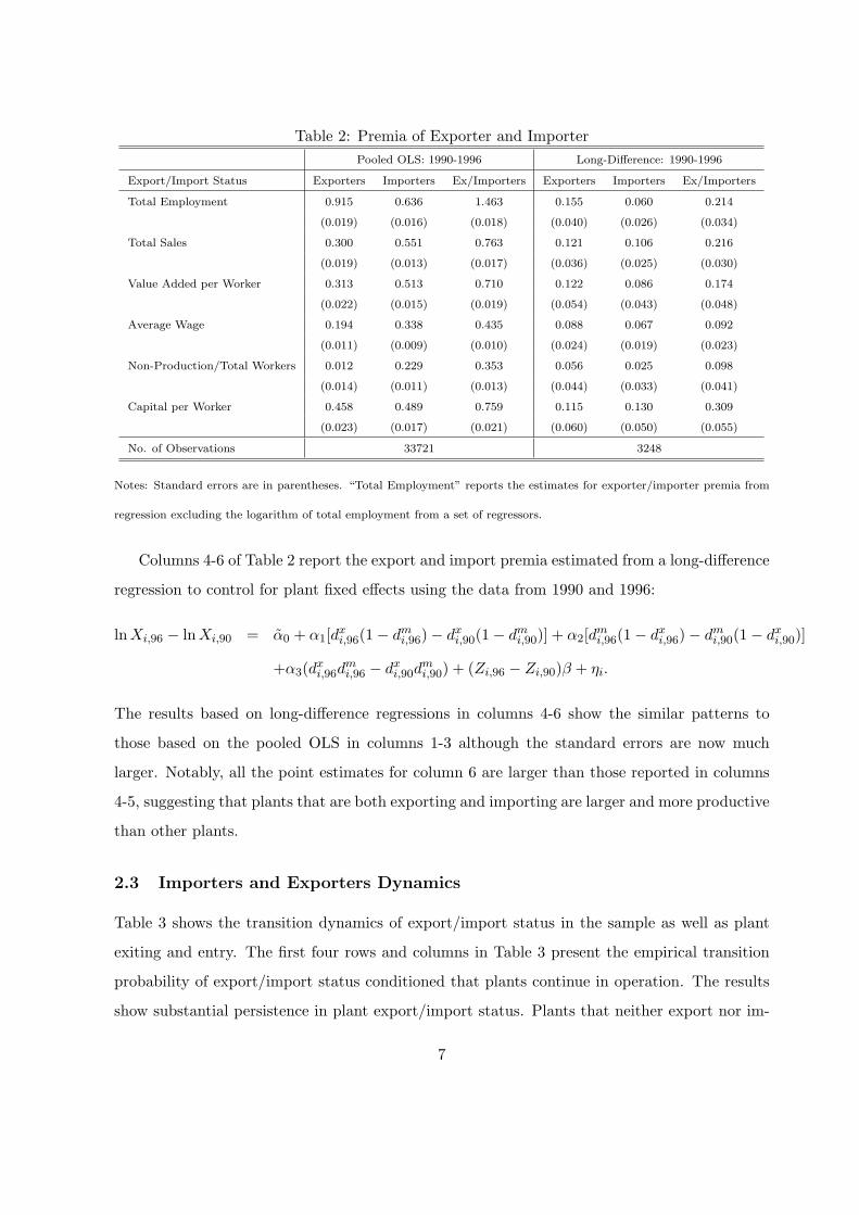
Table 2: Premia of Exporter and ImporterPooled OLS: 1990-1996 Long-Difference: 1990-1996
Export/Import Status Exporters Importers Ex/Importers Exporters Importers Ex/Importers
Total Employment 0.915 0.636 1.463 0.155 0.060 0.214
(0.019) (0.016) (0.018) (0.040) (0.026) (0.034)
Total Sales 0.300 0.551 0.763 0.121 0.106 0.216
(0.019) (0.013) (0.017) (0.036) (0.025) (0.030)
Value Added per Worker 0.313 0.513 0.710 0.122 0.086 0.174
(0.022) (0.015) (0.019) (0.054) (0.043) (0.048)
Average Wage 0.194 0.338 0.435 0.088 0.067 0.092
(0.011) (0.009) (0.010) (0.024) (0.019) (0.023)
Non-Production/Total Workers 0.012 0.229 0.353 0.056 0.025 0.098
(0.014) (0.011) (0.013) (0.044) (0.033) (0.041)
Capital per Worker 0.458 0.489 0.759 0.115 0.130 0.309
(0.023) (0.017) (0.021) (0.060) (0.050) (0.055)
No. of Observations 33721 3248
Notes: Standard errors are in parentheses. “Total Employment” reports the estimates for exporter/importer premia from
regression excluding the logarithm of total employment from a set of regressors.
Columns 4-6 of Table 2 report the export and import premia estimated from a long-difference
regression to control for plant fixed effects using the data from 1990 and 1996:
ln Xi,96 − ln Xi,90 = α0 + α1[dxi,96(1− dm
i,96)− dxi,90(1− dm
i,90)] + α2[dmi,96(1− dx
i,96)− dmi,90(1− dx
i,90)]
+α3(dxi,96d
mi,96 − dx
i,90dmi,90) + (Zi,96 − Zi,90)β + ηi.
The results based on long-difference regressions in columns 4-6 show the similar patterns to
those based on the pooled OLS in columns 1-3 although the standard errors are now much
larger. Notably, all the point estimates for column 6 are larger than those reported in columns
4-5, suggesting that plants that are both exporting and importing are larger and more productive
than other plants.
2.3 Importers and Exporters Dynamics
Table 3 shows the transition dynamics of export/import status in the sample as well as plant
exiting and entry. The first four rows and columns in Table 3 present the empirical transition
probability of export/import status conditioned that plants continue in operation. The results
show substantial persistence in plant export/import status. Plants that neither export nor im-
7

Table 3: Transition Probabilities of Export and Import Status and Entry and Exit
Export/Import Status at t + 1 conditioned on Staying
(1) No-Export (2) Export (3) No-Export (4) Export (2)+(4) (3)+(4) Exit at
/No-Import /No-Import /Import /Import Export Import t + 1a
No-Export/No-Import at t 0.927 0.024 0.042 0.007 0.031 0.048 0.082
Export/No-Import at t 0.147 0.677 0.013 0.163 0.841 0.176 0.070
No-Export/Import at t 0.188 0.017 0.699 0.096 0.113 0.795 0.035
Export/Import at t 0.025 0.101 0.070 0.804 0.905 0.874 0.022
New Entrants at tb 0.753 0.096 0.100 0.051 0.147 0.151 0.126
Empirical Dist. in 1990-96c 0.686 0.086 0.120 0.108 0.194 0.228 0.068
Note: a). “Exit at t + 1” is defined as plants that are observed at t but not observed at t + 1 in the sample. b). “New
Entrants t” is defined as plants that are not observed at t− 1 but observed at t in the sample, of which row represents the
empirical distribution of export/import status at t as well as the probability of not being observed (i.e., exit) at t + 1. c).
“Actual Dist. in 1990-1996” is the empirical distribution of Export/Import Status in 1990-1996.
port, categorized as “No-Export/No-Import,” are very likely (with 92.7% probability) to neither
export nor import next period. Plants that both export and import keep the same status next
period with a relatively high probability of 80.4%. Plants that are either exporting or importing
(but not both) keep the same status with probabilities of 67.7% and 69.9%, respectively, which
is also substantial. The existence of persistence in export/import status suggests the presence
of sunk costs to exporting and importing. 3
Table 3 also indicates that the probability of exporting next period depends on import
status in this period even after controlling for export status. Among non-exporters, in the first
and the third rows of the fifth column of the table, the probability of exporting next period
for importers is 11.3 percent, which is substantially higher than for non-importers, 3.1 percent.
Among exporters, the probability of exporting next period for importers is higher by 6.4 percent
than that for non-importers. Similarly, the probability of importing next period is higher among
exporters than non-exporters even after controlling for importing status. The differences in the
probability of importing next period for exporters are higher than for non-exporters by 12.8
percent among importers and by 7.9 percent among non-importers.
Plants that are engaged in export activities and/or import activities are also more likely to3Unobserved plant-specific characteristics may also lead to persistence in export/import status.
8

survive as shown in the last column of Table 3. While the exiting probability for plants that are
both exporting and importing is only 2.2 percent, plants that are either exporting or importing
(but not both) are more likely to exit next period with probabilities of 7.0 percent and 3.5
percent, respectively. Plants that are neither exporting nor importing have the highest exiting
probability of 8.2 across different export/import status.
Finally, the fifth row of Table 3 reports the empirical distribution of export/import status
as well as the probability of exiting next period among new entrants. Comparing the empirical
distribution of export/import status among all plants reported in the sixth row, new entrants
are less likely to export or import than incumbents; the probabilities of exporting and importing
among new entrants are, respectively, 14.7 percent and 15.1 percent, while the (unconditional)
probabilities of exporting and importing among all plants are, respectively, 19.4 percent and 22.8
percent. New entrants face an exiting probability of 12.6 percent, which is substantially higher
even relative to the exiting probability for plants that are neither exporting nor importing, 8.2
percent.
We now present a static model with heterogeneous firms which is based on Melitz(2003).
We incorporate both exporting of final goods and importing of intermediate goods and allow
for fixed import and export cost complementarities. We use this environment to examine the
impact of trade liberalization on resource reallocation and productivity in the presence of such
complementarities.
3 A Model of Exports and Imports
In this section we extend the trading environment studied by Melitz (2003) to include importing
of intermediates by heterogeneous final goods producers. We demonstrate that the positive
effects of trade on aggregate productivity and welfare due to resource reallocation from less to
more productive firms highlighted by Melitz (2003) is strengthened by the presence of trade in
intermediates. We also explore the effects of the prohibition of imports on export activity and
show that restricting imports leads to a decline in the fraction of operating firms which engage
in exporting.
9

3.1 Environment
The world is comprised of N + 1 countries. Within each country there is a set of final goods
producers and a set of intermediate goods producers. In the open economy, if a final good
producer chooses to export, it will export its good to N countries and if it chooses to import
intermediates, it will import from N countries.
3.1.1 Consumers
There is a representative consumer who supplies labour inelastically at level L. The consumer’s
preferences over consumption of a continuum of final goods are given by:
U =[∫
ω∈Ωq(ω)ρdω
]1/ρ
,
where ω is an index over varieties, and 0 < ρ < 1. The elasticity of substitution is given by
σ = 1/(1− ρ) > 1.
Letting p(ω) denote the price of variety ω, we can derive optimal consumption of variety ω
to be
q(ω) = Q
[p(ω)P
]−σ
, (1)
where P is a price index given by
P =[∫
ω∈Ωp(ω)1−σdω
]1/(1−σ)
, (2)
and Q is a consumption index with Q = U . We also denote aggregate expenditure as R = PQ
and have
r(ω) = R
[p(ω)P
]1−σ
, (3)
where r(ω) is expenditure on variety ω with R =∫ω∈Ω r(ω)dω.
3.1.2 Production
We first describe the final-good sector which is characterized by a continuum of monopolistically
competitive firms selling horizontally differentiated goods. Final goods firms sell to domestic
consumers and in the trading environment choose whether or not to also export their goods to
foreign consumers. In production, final goods producers employ labor, domestically produced
intermediates, and in the trading environment, choose whether or not to also use imported
intermediates.
10
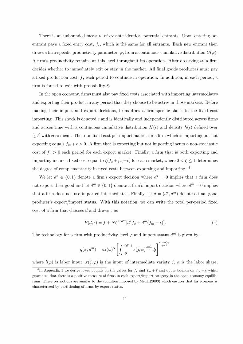
There is an unbounded measure of ex ante identical potential entrants. Upon entering, an
entrant pays a fixed entry cost, fe, which is the same for all entrants. Each new entrant then
draws a firm-specific productivity parameter, ϕ, from a continuous cumulative distribution G(ϕ).
A firm’s productivity remains at this level throughout its operation. After observing ϕ, a firm
decides whether to immediately exit or stay in the market. All final goods producers must pay
a fixed production cost, f , each period to continue in operation. In addition, in each period, a
firm is forced to exit with probability ξ.
In the open economy, firms must also pay fixed costs associated with importing intermediates
and exporting their product in any period that they choose to be active in those markets. Before
making their import and export decisions, firms draw a firm-specific shock to the fixed cost
importing. This shock is denoted ε and is identically and independently distributed across firms
and across time with a continuous cumulative distribution H(ε) and density h(ε) defined over
[ε, ε] with zero mean. The total fixed cost per import market for a firm which is importing but not
exporting equals fm + ε > 0. A firm that is exporting but not importing incurs a non-stochastic
cost of fx > 0 each period for each export market. Finally, a firm that is both exporting and
importing incurs a fixed cost equal to ζ(fx+fm+ε) for each market, where 0 < ζ ≤ 1 determines
the degree of complementarity in fixed costs between exporting and importing. 4
We let dx ∈ 0, 1 denote a firm’s export decision where dx = 0 implies that a firm does
not export their good and let dm ∈ 0, 1 denote a firm’s import decision where dm = 0 implies
that a firm does not use imported intermediates. Finally, let d = (dx, dm) denote a final good
producer’s export/import status. With this notation, we can write the total per-period fixed
cost of a firm that chooses d and draws ε as
F (d, ε) = f + Nζdxdm[dxfx + dm(fm + ε)]. (4)
The technology for a firm with productivity level ϕ and import status dm is given by:
q(ϕ, dm) = ϕl(ϕ)α
[∫ n(dm)
j=0x(j, ϕ)
γ−1γ dj
] (1−α)γγ−1
where l(ϕ) is labor input, x(j, ϕ) is the input of intermediate variety j, α is the labor share,4In Appendix 1 we derive lower bounds on the values for fx and fm + ε and upper bounds on fm + ε which
guarantee that there is a positive measure of firms in each export/import category in the open economy equilib-
rium. These restrictions are similar to the condition imposed by Melitz(2003) which ensures that his economy is
characterized by partitioning of firms by export status.
11
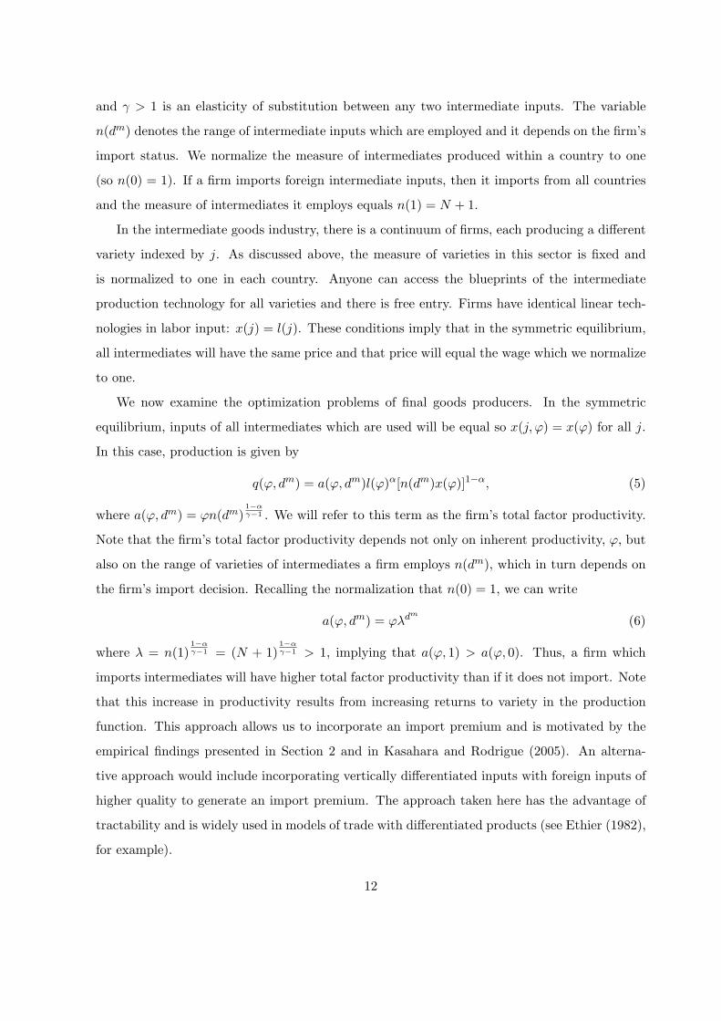
and γ > 1 is an elasticity of substitution between any two intermediate inputs. The variable
n(dm) denotes the range of intermediate inputs which are employed and it depends on the firm’s
import status. We normalize the measure of intermediates produced within a country to one
(so n(0) = 1). If a firm imports foreign intermediate inputs, then it imports from all countries
and the measure of intermediates it employs equals n(1) = N + 1.
In the intermediate goods industry, there is a continuum of firms, each producing a different
variety indexed by j. As discussed above, the measure of varieties in this sector is fixed and
is normalized to one in each country. Anyone can access the blueprints of the intermediate
production technology for all varieties and there is free entry. Firms have identical linear tech-
nologies in labor input: x(j) = l(j). These conditions imply that in the symmetric equilibrium,
all intermediates will have the same price and that price will equal the wage which we normalize
to one.
We now examine the optimization problems of final goods producers. In the symmetric
equilibrium, inputs of all intermediates which are used will be equal so x(j, ϕ) = x(ϕ) for all j.
In this case, production is given by
q(ϕ, dm) = a(ϕ, dm)l(ϕ)α[n(dm)x(ϕ)]1−α, (5)
where a(ϕ, dm) = ϕn(dm)1−αγ−1 . We will refer to this term as the firm’s total factor productivity.
Note that the firm’s total factor productivity depends not only on inherent productivity, ϕ, but
also on the range of varieties of intermediates a firm employs n(dm), which in turn depends on
the firm’s import decision. Recalling the normalization that n(0) = 1, we can write
a(ϕ, dm) = ϕλdm(6)
where λ = n(1)1−αγ−1 = (N + 1)
1−αγ−1 > 1, implying that a(ϕ, 1) > a(ϕ, 0). Thus, a firm which
imports intermediates will have higher total factor productivity than if it does not import. Note
that this increase in productivity results from increasing returns to variety in the production
function. This approach allows us to incorporate an import premium and is motivated by the
empirical findings presented in Section 2 and in Kasahara and Rodrigue (2005). An alterna-
tive approach would include incorporating vertically differentiated inputs with foreign inputs of
higher quality to generate an import premium. The approach taken here has the advantage of
tractability and is widely used in models of trade with differentiated products (see Ethier (1982),
for example).
12

It is well-known that the form of preferences implies that final goods producers will price at
a constant markup equal to 1/ρ over marginal cost. Hence, using the final goods technology and
recalling that all intermediates are priced at the wage which equals one, we have the following
pricing rule for final goods sold in the home market for a producer with productivity ϕ and
import status dm:
ph(ϕ, dm) =(
1ρ
) (1
Γa(ϕ, dm)
), (7)
where Γ ≡ αα(1− α)1−α. Note that the prices in the closed economy equilibrium are just given
by equation (7) with dm = 0.
We also assume that there are iceberg exporting costs so that τ > 1 units of goods has to
be shipped abroad for 1 unit to arrive at its destination. The pricing rule for final goods sold in
the foreign market then is given by:
pf (ϕ, dm) = τph(ϕ, dm) (8)
The total revenue of a final good producer depends on inherent productivity and export/import
status. Using equation (3), revenue from sales in the home market can be written as
rh(ϕ, dm) = R (PρΓa(ϕ, dm))σ−1 (9)
and revenue from foreign sales per country of export is given by
rf (ϕ, d) = dxτ1−σrh(ϕ, dm). (10)
Hence, total revenue for a firm with inherent productivity ϕ and export/import status d is given
by
r(ϕ, d) = rh(ϕ, dm) + Nrf (ϕ, d), (11)
or
r(ϕ, d) = (1 + dxNτ1−σ)rh(ϕ, dm). (12)
Thus, using equations (6), (9), and (12), we can determine revenue for a firm with inher-
ent productivity ϕ and export/import status d relative to a firm with the same productivity
parameter who is neither exporting nor importing:
r(ϕ, d) = bdx
x bdm
m r(ϕ, 0, 0), (13)
13
where bx ≡ 1 + Nτ1−σ and bm ≡ λσ−1.
Turning to profits, we see that the pricing rule of firms implies that profits of a final good
producer with inherent productivity ϕ, export/import status d, and fixed import cost shock ε
can be written as
π(ϕ, d, ε) =r(ϕ, d)
σ− F (d, ε) (14)
In what follows, we explore the equilibria of four economies: the closed economy and three
trading economies. Let autarkic equilibrium variables be denoted with a subscript A and note
that in this equilibrium firms can only choose d = (0, 0). We denote equilibrium variables in the
full trading equilibrium with both importing and exporting with a subscript T . It is also useful
to consider variants of the economy which are characterized by partial trade. In particular, our
open economy with ζ = bm = 1 is equivalent to the open economy studied by Melitz (2003)
with exporting of final goods but no importing of intermediates and we denote this economy
with an X subscript. We also examine an economy with importing of intermediate goods but
no exporting of final goods by evaluating our open economy with ζ = bx = 1. We denote
equilibrium variables of this economy with an I subscript.
Thus, equilibrium levels of the aggregate price index and aggregate revenue in economy
S ∈ A, T,X, I are denoted PS and RS respectively. Evaluating equation (9) at these equilib-
rium values in the relevant economies and using this in equation (12) allows us to determine
equilibrium revenue functions for final goods producers in each economy. We denote these
revenue functions as rS(ϕ, d) for S ∈ A, T, X, I. Similarly, we can derive profit functions,
πS(ϕ, d, ε) for each economy from equation (14).
3.2 Exit, Export, and Import Decisions
3.2.1 Exit Decision
We focus on stationary equilibria in which aggregate variables remain constant over time. Under
the assumptions of no discounting, that the productivity level for a firm is constant throughout
its life, and that the fixed import cost shocks are independent across time, a final goods firm
faces a static optimization problem. In the closed economy, after observing its productivity, a
firm will choose to exit if its period profits are negative. In the open economy, after observing
its productivity, a firm will choose to exit if its expected period profits are negative where the
14
expectation is taken over the stochastic component of the fixed cost of importing, ε.
Each firm’s value function in economy S ∈ A, T, X, I is given by
VS(ϕ) = max
0,
∞∑
t=0
(1− ξ)tEεt
(max
dt∈0,12πS(ϕ, dt, εt)
)= max
0, Eε
(max
d∈0,12πS(ϕ, d, ε)
ξ
).
(15)
In this equation, the second equality follows because ε is independently distributed over time.
Now since profits are strictly increasing in ϕ, there exists a ϕ∗S such that a firm will exit if ϕ < ϕ∗S
where ϕ∗S is characterized by
Eε
(max
d∈0,12πS(ϕ∗S, d, ε)
ξ
)= 0. (16)
or ∫ ε
εmax
d∈0,12πS(ϕ∗S, d, ε)h(ε)dε = 0. (17)
For tractability, we impose lower bounds on ε so that firms with the marginal productivity
for operation in the three open economies will choose to neither import nor export. These
bounds are presented in Appendix 1. Under these bounds, we have the following proposition
which characterizes the cutoff productivities in the four economies considered.
Proposition 1
If the cutoff productivities for operation in each economy are unique, then these cutoff
productivities satisfy rS(ϕ∗S, 0, 0) = σf , for S ∈ A, T, X, I.The proof of this and all remaining propositions are presented in Appendix II. Below, we will
prove that the cutoff productivities are unique.
Note that in each economy, we can relate all other firms’ revenues to the revenues of the
marginal firm for operation in that economy. Using equations (6), (9), and (13), we can derive
in the closed economy ∀ ϕ:
rA(ϕ, 0, 0) =[
ϕ
ϕ∗A
]σ−1
σf. (18)
While in the full trading economy, we can write ∀ (ϕ, d)
rT (ϕ, d) = bdx
x bdm
m
[ϕ
ϕ∗T
]σ−1
σf. (19)
Similarly, for the partial trading economies, we have ∀ (ϕ, dx)
rX(ϕ, dx, 0) = bdx
x
[ϕ
ϕ∗X
]σ−1
σf. (20)
15

and ∀ (ϕ, dm)
rI(ϕ, 0, dm) = bdm
m
[ϕ
ϕ∗I
]σ−1
σf. (21)
3.2.2 Export and Import Decisions
For the full trading economy, we now consider the export and import decisions for firms which
choose not to exit. Recall that firms make exit decisions before observing ε but make export
and import decisions after observing ε. Define the following:
Φ(ϕ) ≡(
ϕ
ϕ∗T
)σ−1 (f
N
), (22)
For convenience, we can reference firms of different productivity levels by Φ where the depen-
dence on ϕ is understood. We will refer to this variable as relative productivity. Thus, using
equations (14) and (19), we can write profits in terms of Φ:
π(Φ, d, ε) = N(bdx
x
) (bdm
m
)Φ− F (d, ε) (23)
To obtain the export and import decision rules as a function of a firm’s productivity and fixed
import cost, we define the following variables.
Let Φdm
x (ε) be implicitly defined by π(Φdm
x (ε), 1, dm, ε) = π(Φdm
x (ε), 0, dm, ε) or
Φdm
x (ε) =ζdm
fx + dm(ζdm − 1)(fm + ε)bdm
m (bx − 1). (24)
So a firm with import status dm, fixed import cost shock ε, and relative productivity Φdm
x (ε)
will be indifferent between exporting and not exporting. Let Φdx
m (ε) be implicitly defined by
π(Φdx
m (ε), dx, 1, ε) = π(Φdx
m (ε), dx, 0, ε) or
Φdx
m (ε) =ζdx
(fm + ε) + dx(ζdx − 1)fx
bdx
x (bm − 1). (25)
So a firm with export status dx, fixed import cost shock ε, and relative productivity Φdx
m (ε)
will be indifferent between importing and not importing. Let Φxm(ε) be implicitly defined by
π(Φxm(ε), 1, 1, ε) = π(Φxm(ε), 0, 0, ε) or
Φxm(ε) =ζ(fx + fm + ε)
(bxbm − 1). (26)
So a firm with fixed import cost shock ε, and relative productivity Φxm(ε) will be indifferent
between participating in both exporting and importing markets and not participating in either
market.
16

These variables allow us to determine the firms’ choices of d depending on their Φ and their
ε. If we let θ ≡ fm + ε, where θ ∈ (fm + ε, fm + ε) ≡ (θ, θ), then we can graph each of the
variables defined in equations (24), (25), and (26) above as a function of θ, and determine
firms’ export and import choices depending on their relative productivity, Φ, and the random
component of their fixed import cost, ε. We first consider the case with no complementarities
in fixed export and import costs, ζ = 1. Figure 1 graphs cutoff functions for this case and
shows the four regions of possible export/import status. Note that Φ(ϕ∗T ) = fN so active firms
are those with Φ ≥ fN . As the figure demonstrates, the space of (Φ, θ) is partitioned into four
areas according to firms’ export and import choices. Firms with relatively low productivity and
low fixed cost of importing will choose to import but not export. Firms with relatively low
productivity and higher fixed cost of importing will choose to neither import nor export. Firms
with relatively high productivity and relatively high fixed cost of importing will choose to export
but not import. Finally, firms with relatively high productivity will choose to both import and
export.
By examining the equations for the different regions, we can also determine the effect of
complementarities in the fixed costs of importing and exporting. Recall that a decrease in ζ
represents an increase in complementarities. Examination of equations (24)-(26) shows that a
decrease in ζ will shift down and decrease the slopes of Φ1m(·), Φ1
x(·), and Φxm(·). As can be seen
from Figure 2, each of these changes would serve to increase the measure of firms choosing to
both export and import and decrease the measure of firms in each of the other three areas. This
is intuitive as an increase in the complementarities in fixed costs of importing and exporting
should increase the fraction of firms which choose to engage in both activities.
3.3 Aggregation
In this section, we derive a weighted average of firm productivity levels for each of the four types
of economies. As in Melitz(2003), these averages will also represent aggregate productivity in
each environment because they summarize the information in the distribution of productivities
which are relevant for aggregate variables.
Let νS(ϕ∗S, d) denote the fraction of successful firms that have export/import status equal to
d in economy S ∈ A, T, X, I. These fractions are presented in Appendix I. Furthermore, let
MS(ϕ∗S) denote the equilibrium mass of operating firms in economy S. With these variables, we
17
can derive the total mass of firms with export/import status equal to d in each economy as
MS(ϕ∗S, d) = νS(ϕ∗S, d)MS(ϕ∗S) (27)
Hence, the total number of varieties available to a consumer in each equilibrium is given by
MCS (ϕ∗S) = MS(ϕ∗S) + N [MS(ϕ∗S, 1, 0) + MS(ϕ∗S, 1, 1)], where MS(ϕ∗S) varieties are purchased
from home producers and N(MS(ϕ∗S, 1, 0) + MS(ϕ∗S, 1, 1)) are purchased from foreign producers
(imported final goods).
We demonstrate in Appendix I that the aggregate price index given by equation (2) for
each economy can be written as a function of a weighted average of the productivities of all
firms (home and foreign) from which a consumer purchases final goods. Let bS(ϕ∗S, d) denote
this weighted average across firms choosing export/import status d in economy S ∈ A, T,X, Ifrom which the consumer purchases final goods. The price index in economy S as a function of
these average productivities is given by:
PS =[
1Γρ
] ∑
d∈0,12MS(ϕ∗S, d)bS(ϕ∗S, d)σ−1
11−σ
(28)
or
PS = MCS (ϕ∗S)
11−σ p
1
MCS (ϕ∗S)
∑
d∈0,12MS(ϕ∗S, d)bS(ϕ∗S, d)σ−1
11−σ
(29)
This equation implies that the aggregate price level can be written as a function of the number
of varieties available to the consumer (MCS (ϕ∗S)) and a weighted average of productivities of all
operating firms given by:
bS(ϕ∗S) =
1
MCS (ϕ∗S)
∑
d∈0,12MS(ϕ∗S, d)bS(ϕ∗S, d)σ−1
1σ−1
(30)
This measure of average productivity summarizes the effects of the distribution of productivity
levels and fixed import costs on aggregate outcomes.
Hence, we can write the aggregate price level in each economy as
PS =MC
S (ϕ∗S)1
1−σ
ΓρbS(ϕ∗S). (31)
Furthermore, using equations (3), (18), (19), (20), (21), (30), and the average productivity
measures defined in Appendix I, we can write aggregate revenue in each economy as
RS = MCS (ϕ∗S)rS(bS(ϕ∗S), 0, 0) (32)
18
3.4 Autarkic and Trading Equilibria
As the above analysis suggests, all variables in the stationary equilibrium for each economy can
be determined once we determine the cutoff variable for operation, ϕ∗S. We now seek to charac-
terize the equations which determine these cutoff variables in each of the four economies under
consideration. Let average profits within each group of firms according to export/import status
in economy S be denoted πS(ϕ∗S, d). These average profit functions are derived in Appendix I.
Note that the average profits for each group are derived under the equilibrium condition that
expected profits for the marginal firm equal zero.
Thus, for each economy we have our first equilibrium equation in two unknowns: average
overall profit and the cutoff productivity:
πS(ϕ∗S) =∑
d∈0,12νS(ϕ∗S, d)πS(ϕ∗S, d). (33)
The second equilibrium equation for each economy is given by the free-entry condition which
guarantees that the ex-ante value of an entrant must be equal zero:
(1−G(ϕ∗S))(
πS(ϕ∗S)ξ
)− fe = 0. (34)
Combining equations (33) and (34) determines the equilibrium cutoff productivity for exit in
each economy, ϕ∗S:∑
d∈0,12νS(ϕ∗S, d)π(ϕ∗S, d) =
ξfe
(1−G(ϕ∗S)). (35)
Proposition 2
The four equilibria cutoff productivities, ϕ∗A, ϕ∗X , ϕ∗I , and ϕ∗T exist and are unique.
The following proposition examines the impact of various forms of trade on the cutoff pro-
ductivity level for operation.
Proposition 3
(i.) ϕ∗A < ϕ∗X < ϕ∗T .
(ii.) ϕ∗A < ϕ∗I < ϕ∗T .
We also note that equation (34) and this proposition implies that average profits have a similar
ranking across the different economies. This proposition implies that opening trade in either final
goods or intermediates or both causes firms with lower productivity to exit. In the economy with
19
no importing, this result is identical to that identified by Melitz(2003) where the exportation
of final goods generates a resource reallocation from less productive firms to more productive
firms. In the economy with only importing, there is also exit of less productive firms and this,
along with the importing of foreign intermediates in the presence of increasing returns to variety,
causes aggregate productivity to increase. In the full trading equilibrium, both effects are at
work and the reallocation from less productive firms to more productive firms is intensified and
aggregate productivity increases.
We now state a number of propositions which examine the impact of moving from autarky
to an economy with trade on this measure of welfare and other aggregate variables of interest.
Proposition 4
(i.) MA > MX > MT
(ii.) MA > MI > MT
This result is also similar to Melitz (2003) and results as the supply of labor is fixed but more
productive firms now demand more labour so some firms must exit. This is an example of a
selection effect as discussed in the trade literature with increasing returns and free entry (see
Krugman (1979), for example.) Our environment identifies an additional mechanism arising
from the presence of imported intermediates that strengthens the selection effect discussed by
Melitz (2003). Note also that the number of varieties available to the consumer in the open
economies may be higher or lower than the number of varieties available to the consumer in
autarky.
We are also interested in the normative effects of trade and we can use the equilibrium
aggregate price index in each equilibrium to calculate welfare per worker:
WS =1PS
. (36)
In moving from autarky to an economy with trade in final goods, consumer welfare is impacted
by two effects. The number of varieties available to the consumer changes and aggregate produc-
tivity is higher. In the trading economy with no trade in final goods but trade in intermediates,
consumer welfare is only affected by the latter effect. The aggregate productivity gain impacts
positively on welfare. If the number of varieties available to the consumer is higher in trade then
welfare is also enhanced by this effect but if it falls then welfare is negatively impacted. However,
the next proposition states that the increase in welfare from the productivity gain dominates
20
and welfare is higher in any of the trading economies than in autarky It also demonstrates that
full trade generates higher welfare than partial trade.
Proposition 5
(i.) WA < WX < WT
(ii.) WA < WI < WT
We now examine the effect of trade on firms’ revenues and profits. As in Melitz(2003), we
compare revenues and profits of a firm with a given level of productivity between autarky and
trade. Recalling that RS = L ∀S ∈ A, T, X, I, we note that a firm’s market share within the
home country just equals its revenue in each equilibrium. Thus, comparing revenues is also a
comparison of market shares. The next proposition argues that trade shifts market shares from
firms which do not engage in trade in the open economy to firms which do. In what follows let
rA(ϕ) and πA(ϕ) denote the revenue and profits of a firm in autarky with inherent productivity
ϕ.
Proposition 6
Let bx and bm be defined by ϕ∗T (bx) = b1
σ−1m ϕ∗A and ϕ∗T (bm) = b
1σ−1x ϕ∗A. Consider a firm with
productivity ϕ, then comparing revenue of this firm between autarky and trade, we have the
following results:
(i.) rT (ϕ, 0, 0) < rA(ϕ) < rT (ϕ, 1, 1)
(ii.) rA(ϕ)≤>rT (ϕ, 1, 0) as bm≤> bm
(iii.) rA(ϕ)≤>rT (ϕ, 0, 1) as bx≤> bx
In the proof of this proposition we demonstrate that bx > 1 and bm > 1. Thus when
ζ = bm = 1 (an economy with no intermediate imports) firms which choose to export in the
open economy have higher revenues than they did in autarky (this result is analogous to the
revenue comparison in Melitz(2003)). Similarly, when ζ = bx = 1 (no final goods exports), firms
which choose to import in the open economy have higher revenues than they did in autarky.
In the economy with both exports and imports, (ii.) implies that if the returns to importing
are large enough, then a firm which chooses to export but not import in the open economy will
lose revenue. The intuition for this result is that a firm which chooses to only export is at a
disadvantage relative to its domestic and foreign competitors who are importing intermediates
and gaining in productivity. If the returns to importing are large (bm large) then the presence
21

of these competitors leads to lower market shares for a firm which is only exporting. We have a
similar effect for firms which are only importing if the returns to exporting are high (bx large).
The next proposition compares the profits for firms between autarky and trade.
Proposition 7
(i.) πT (ϕ, 0, 0, ε) < πA(ϕ) ∀ϕ, ∀ε(ii.) ∃ ϕT (ε) > ϕ∗T such that πT (ϕ, 1, 1, ε)≤>πA(ϕ) as ϕ≤> ϕT (ε), ∀ ε
(iii.) For bm ≤ bm, ∃ ϕX > ϕ∗T such that πT (ϕ, 1, 0, ε)≤>πA(ϕ) as ϕ≤> ϕX , ∀ ε
For bm > bm, πT (ϕ, 1, 0, ε) < πA(ϕ), ∀ ϕ, ∀ ε
(iv.) For bx ≤ bx, ∃ ϕM (ε) > ϕ∗T such that πT (ϕ, 0, 1, ε)≤>πA(ϕ) as ϕ≤> ϕM (ε), ∀ ε
For bx > bx, πT (ϕ, 0, 1, ε) < πA(ϕ), ∀ ϕ, ∀ ε
The first statement in this proposition follows because firms which neither export nor import in
the open economy lose revenue so must have lower profits in trade than in autarky. The second
part of this proposition states that trade allows the most efficient firms (higher productivity
and lower fixed costs of importing) to fully engage in trade and gain market share and profits.
However, we know that for a firm with ε1 < ε < ε2 and ϕ = ϕxm(ε) that this firm will fully
engage in trade but will have lower profits in trade than in autarky. Hence, only a subset of
firms which choose to both import and export in the open economy will have higher profits than
in autarky.
Part (iii.) of the proposition suggests the possibility of a similar partitioning among firms
which only export in the open economy. If the returns to importing are not too high, then
all firms which choose to only export in the open economy will have higher market share but
possibly some of those firms will have lower profits while others have higher profits. Part (iv.) of
the proposition states a similar result for firms which only import in the open economy. Figures
4-6 exhibit the revenue and profit comparisons contained in Propositions 6 and 7.
3.5 Import Restrictions
We now briefly examine the effects on export activity of import restrictions. In this environment,
the importation of intermediates makes firms more productive because of the increasing returns
to variety in production. This may allow a larger fraction of firms to cover the fixed cost
associated with exporting and allow them to enter the export market. Thus, a restriction on
imports may decrease export activity and hence, import protection may act as export destruction
22
in this environment.
Recall from equation (6) that a firm’s total factor productivity is given by
a(ϕ, dm) = ϕλdm(37)
where λ = n(1)1−αγ−1 > 1. We model import restrictions as a decrease in the number of import
markets to which firms have access – that is a decrease in n(1) (which we previously assumed
equaled the number of a country’s trading partners). Hence an import restriction will be modeled
as a decrease in λ and a resulting decrease in bm = λσ−1. In what follows, we seek to determine
the effect of a decrease in bm on a measure of export activity in the full trading equilibrium.
Proposition 8
In the full trading equilibrium, the fraction of firms which export and the average revenue and
market share of exporting firms is increasing in bm.
Figure 3 demonstrates the effect on the fraction of exporters when there are no fixed cost
complementarities (ζ = 1) for the extreme case in which imports are prohibited (bm → 1). The
hatched area in that figure shows the fraction of exporting firms which stop exporting when
imports are prohibited, and, hence the export destruction due to import protection.
It should also be clear that restricting imports of intermediates will lower aggregate produc-
tivity in this environment. This will result from a direct effect and an indirect effect. The direct
effect is clear from the above discussion and equation (6), which demonstrates that importing
intermediates increases productivity because of increasing returns to variety in production. As
Proposition 3 demonstrates, there will also be an indirect negative effect on aggregate pro-
ductivity because restricting imports decreases the average cutoff productivity for operation
so resources will be reallocated from more productive firms toward less productive firms and
aggregate productivity will fall.
4 Structural Estimation of Static Model
4.1 The Environment
In this section, we develop an empirical model based on the theoretical model in the previous
section. We add additional shocks to the model but the fundamental environment remains the
same. In particular we introduce a stochastic fixed cost of exporting, similar to the fixed cost
23

of importing in the model above to retain symmetry between these two activities. We also
incorporate a cost shocks associated with exiting to improve the estimation.
We make the following distributional assumptions:
• The logarithm of plant-specific productivity upon entry is drawn from N(0, σ2ϕ).5 Produc-
tivity is constant after the initial draw.
• The cost shocks associated with the export/import decision, denoted by εdt (d) for d ∈
0, 12, are independently drawn from the identical extreme-value distribution with mean
zero and scale parameter %d. Let εdt ≡ (εd
t (0, 0), εdt (1, 0), εd
t (0, 1), εdt (1, 1)).
• The cost shocks associated with the exiting decision, denoted by εχt = (εχ
t (0), εχt (1)), are
independently drawn from the identical extreme-value distribution with mean zero and
scale parameter %χ.
The discount factor is given by β ∈ (0, 1). The timing of the incumbent’s decision with the
productivity ϕ within each period is as follows. At the beginning of every period, a firm faces a
possibility of a large negative shock that leads it to exit with an exogenous probability ξ. Then,
a firm draws the (additional) choice-dependent idiosyncratic cost shocks associated with exiting
decisions, εχt = (εχ
t (0), εχt (1)). Given the realizations, the firm decides whether it exits from the
market or continues to operate. If the firm decides to exit, it receives the terminal value of εχt (0).
If the firm decides to continue to operate, then it will draw the choice-dependent idiosyncratic
cost shocks associated with export and import, εdt (d) for d ∈ 0, 12. After observing εd
t (d), the
firm makes export and import decisions. The Bellman’s equation for an incumbent firm with
the productivity ϕ is written as
V (ϕ) =∫
maxεχ′(0),W (ϕ) + εχ′(1)dHχ(εχ′)
W (ϕ) =∫
maxd∈0,12
π(ϕ, d) + β(1− ξ)V (ϕ) + εd′(d)
dHd(εd′),
or, using the properties of the extreme-value distributed random variables [c.f., Rust (1987)],
the Bellman’s equation is rewritten as
V (ϕ) = %χ ln(exp(0) + exp(W (ϕ)/%χ))
W (ϕ) = %d ln
(∑
d′exp
([π(ϕ, d′) + β(1− ξ)V (ϕ)]/%d
)). (38)
5The mean of initial productivity draws is set to zero in order to achieve the identification.
24
With the solution to the functional equation (54), the conditional choice probabilities of
exiting and export/import decisions follow the Nested Logit formula. In particular, taking into
account the exogenous exiting probability of ξ, the probability of exiting (χ = 0) and staying
(χ = 1) is given by:
P (χ = 1|ϕ) = (1− ξ)exp(W (ϕ)/%χ)
exp(0) + exp(W (ϕ)/%χ), (39)
and P (χ = 0|ϕ) = 1 − P (χ = 1|ϕ). Conditional on χ = 1 (i.e., continuously operating), the
choice probabilities of d are given by the multinomial logit formula:
P (d|ϕ, χ = 1) =exp([π(ϕ, d) + β(1− ξ)V (ϕ)]/%d)∑
d′∈0,12 exp([π(ϕ, d′) + β(1− ξ)V (ϕ)]/%d), (40)
4.2 Stationary Equilibrium
As before, we focus on a stationary equilibrium in which the distribution of ϕ is constant over
time and let the stationary distribution of ϕ among incumbents is denoted by µ(ϕ).
The expected value of an entering firm is given by∫
V (ϕ′)g0(ϕ′)dϕ′, where V (·) is given in
(54). Under free entry, this value must be equal to the fixed entry cost fe:
∫V (ϕ′)gϕ(ϕ′)dϕ′ = fe,
where gϕ(ϕ) = φ(ϕ/σϕ)/σϕ. In equilibrium, this free entry condition has to be satisfied.
The stationarity requires that, for each productivity-type ϕ, the number of exiting firms is
equal to the number of successful new entrants so that:
MP (χ = 1|ϕ)µ(ϕ) = MeP (χ = 0|ϕ)gϕ(ϕ),
where M is a total mass of incumbents; Me is a mass of new entrants. This implies that the
stationary distribution µ can be computed as:
µ(ϕ) =Me
M
P (χ = 1|ϕ)P (χ = 0|ϕ)
gϕ(ϕ),
where, using∫
dµ(ϕ) = 1, we may derive
Me
M=
1∫ P (χ=1|ϕ)
P (χ=0|ϕ)gϕ(ϕ)dϕ.
25

4.3 Likelihood Function
The total revenue and the export revenue are assumed to be measured with errors, denoted by
ωit and ωfit, where ωit is a measurement error for total revenue and ωf
it is a measurement error
for export revenue. We also consider labor augmented technological change at the annual rate
of αt. Modifying the revenue functions by incorporating measurement errors (ωit, ωfit) and time
trend αt, we specify the logarithm of the observed total and export revenues as:
ln rit = α0 + αtt + log[1 + exp(αx)dxit] + αmdm
it + ln ϕi + ωit (41)
ln rfit = α0 + αtt + αx + αmdm
it + lnϕi + ωfit, (42)
where ωit is measurement error in total revenue and ωit is measurement error in export revenue.
Importantly, equations (41)-(42) are reduced-form specifications; we have the following rela-
tionships between reduced-form parameters and structural parameters:6
α0 = ln[αα(1− α)1−αRP σ−1],
αx = ln[Nτ1−σ],
αm = (σ − 1) ln λ.
Note that, since α0, αx, and αm are not structural parameters, they could be affected by policy
changes. In particular, any policy change that will affect the aggregate price P will lead to
a change in α0. As we discuss later, counterfactual policy experiments we conduct in this
paper explicitly take into account for equilibrium price responses using our knowledge on the
relationship between the reduced form parameter α0 and the aggregate price P .
Given these specifications for revenues, firm’s profit is
π(ϕi, dit) = (1/σ)r(ϕi, dit)− F (dit), (43)
where
r(ϕi, dit) = [1 + exp(αx)dxit] exp(α0 + αmdm
it + ln ϕi)
F (dit) = f + ζdx
itdmit
f (fxdxit + fmdm
it ).
6Also, with abuse of notation, we replace (σ− 1) ln ϕ by ln ϕ since (σ− 1) cannot be separately identified from
the variance of ln ϕ.
26
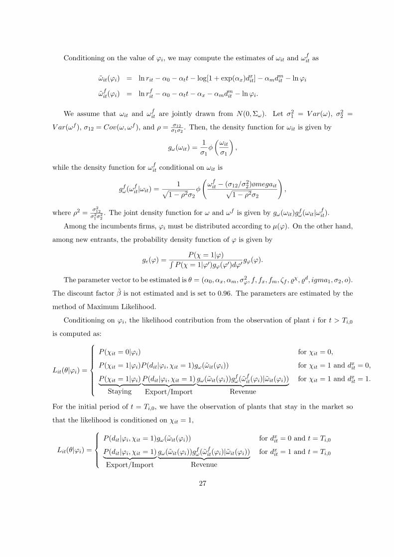
Conditioning on the value of ϕi, we may compute the estimates of ωit and ωfit as
ωit(ϕi) = ln rit − α0 − αtt− log[1 + exp(αx)dxit]− αmdm
it − lnϕi
ωfit(ϕi) = ln rf
it − α0 − αtt− αx − αmdmit − ln ϕi.
We assume that ωit and ωfit are jointly drawn from N(0,Σω). Let σ2
1 = V ar(ω), σ22 =
V ar(ωf ), σ12 = Cov(ω, ωf ), and ρ = σ12σ1σ2
. Then, the density function for ωit is given by
gω(ωit) =1σ1
φ
(ωit
σ1
),
while the density function for ωfit conditional on ωit is
gfω(ωf
it|ωit) =1√
1− ρ2σ2
φ
(ωf
it − (σ12/σ22)ømegait√
1− ρ2σ2
),
where ρ2 = σ212
σ21σ2
2. The joint density function for ω and ωf is given by gω(ωit)gf
ω(ωit|ωfit).
Among the incumbents firms, ϕi must be distributed according to µ(ϕ). On the other hand,
among new entrants, the probability density function of ϕ is given by
ge(ϕ) =P (χ = 1|ϕ)∫
P (χ = 1|ϕ′)gϕ(ϕ′)dϕ′gϕ(ϕ).
The parameter vector to be estimated is θ = (α0, αx, αm, σ2ϕ, f, fx, fm, ζf , %χ, %d, igma1, σ2, o).
The discount factor β is not estimated and is set to 0.96. The parameters are estimated by the
method of Maximum Likelihood.
Conditioning on ϕi, the likelihood contribution from the observation of plant i for t > Ti,0
is computed as:
Lit(θ|ϕi) =
P (χit = 0|ϕi) for χit = 0,
P (χit = 1|ϕi)P (dit|ϕi, χit = 1)gω(ωit(ϕi)) for χit = 1 and dxit = 0,
P (χit = 1|ϕi)︸ ︷︷ ︸Staying
P (dit|ϕi, χit = 1)︸ ︷︷ ︸Export/Import
gω(ωit(ϕi))gfω(ωf
it(ϕi)|ωit(ϕi))︸ ︷︷ ︸Revenue
for χit = 1 and dxit = 1.
For the initial period of t = Ti,0, we have the observation of plants that stay in the market so
that the likelihood is conditioned on χit = 1,
Lit(θ|ϕi) =
P (dit|ϕi, χit = 1)gω(ωit(ϕi)) for dxit = 0 and t = Ti,0
P (dit|ϕi, χit = 1)︸ ︷︷ ︸Export/Import
gω(ωit(ϕi))gfω(ωf
it(ϕi)|ωit(ϕi))︸ ︷︷ ︸Revenue
for dxit = 1 and t = Ti,0
27
The likelihood contribution from plant i conditioned on ϕi is
Li(θ|ϕi) =Ti,1∏
Ti,0
Lit(θ|ϕi).
Since we do not observe ϕi, we integrate out the unobserved ϕi to compute the likelihood
contribution from plant i observation. The distribution of ϕi crucially depends on whether a
plant is observed in the initial sample period or not. If plant i is observed in the initial sample
period, we integrate out ϕi using the stationary distribution µ(ϕ) while, if plant i enters into the
sample after the initial sample period, we use the distribution of initial draws upon successful
entry ge(ϕ). Thus,
Li(θ) =
∫Li(θ|ϕ′)µ(ϕ′)dϕ′ for Ti,0 = 1990,
∫Li(θ|ϕ′)ge(ϕ′)dϕ′ for Ti,0 > 1990.
The parameter vector θ can be estimated by maximizing the logarithm of likelihood function
L(θ) =N∑
i=1
lnLi(θ). (44)
Evaluation of the log-likelihood involves solving computationally intensive dynamic program-
ming problem that approximates the Bellman equation (54) by discretization of state space. For
each candidate parameter vector θ, we solve the discretized version of (54) and then obtain the
choice probabilities, (55) and (56), as well as the stationary distribution from the associated
policy function. Once the choice probabilities and the stationary distribution are obtained for a
particular candidate parameter vector θ, then we may evaluate the log-likelihood function (61).
Repeating this process, we can maximize (61) over the parameter vector space of θ to find the
estimate.
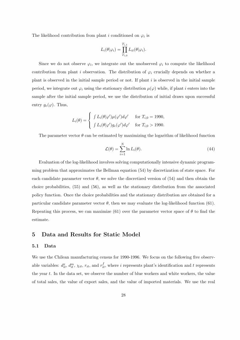
5 Data and Results for Static Model
5.1 Data
We use the Chilean manufacturing census for 1990-1996. We focus on the following five observ-
able variables: dxit, dm
it , χit, rit, and rfit, where i represents plant’s identification and t represents
the year t. In the data set, we observe the number of blue workers and white workers, the value
of total sales, the value of export sales, and the value of imported materials. We use the real
28
values of total sales and export sales, respectively, for rit and rfit where the manufacturing output
price deflator is used to convert the nominal value into the real value. The export/import status,
(dmit , d
xit), is identified from the data by checking if the value of export sales and/or the value
of imported materials are zero or positive. The entry/exiting decisions, χit, can be identified
in the data by looking at the number of workers across years. We use unbalanced panel data
of 7234 plants for 1990-1996, including all the plants that has been observed at least one year
between 1990 and 1996: dxit, d
mit , χit, r
hit, r
fitTi,1
t=Ti,07234
i=1 . Here, Ti,0 is the first year in which firm
i appears in the data, which is either 1990 or the year in which firm i entered between 1991 and
1996. Ti,1 is the last year in which firm i appears in the data, which is either 1996 or the year
in which firm i exited between 1991 and 1995.
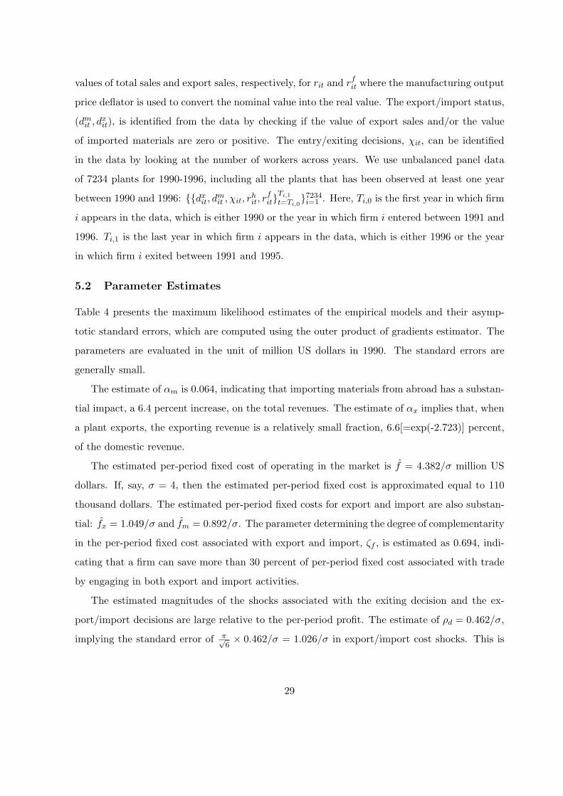
5.2 Parameter Estimates
Table 4 presents the maximum likelihood estimates of the empirical models and their asymp-
totic standard errors, which are computed using the outer product of gradients estimator. The
parameters are evaluated in the unit of million US dollars in 1990. The standard errors are
generally small.
The estimate of αm is 0.064, indicating that importing materials from abroad has a substan-
tial impact, a 6.4 percent increase, on the total revenues. The estimate of αx implies that, when
a plant exports, the exporting revenue is a relatively small fraction, 6.6[=exp(-2.723)] percent,
of the domestic revenue.
The estimated per-period fixed cost of operating in the market is f = 4.382/σ million US
dollars. If, say, σ = 4, then the estimated per-period fixed cost is approximated equal to 110
thousand dollars. The estimated per-period fixed costs for export and import are also substan-
tial: fx = 1.049/σ and fm = 0.892/σ. The parameter determining the degree of complementarity
in the per-period fixed cost associated with export and import, ζf , is estimated as 0.694, indi-
cating that a firm can save more than 30 percent of per-period fixed cost associated with trade
by engaging in both export and import activities.
The estimated magnitudes of the shocks associated with the exiting decision and the ex-
port/import decisions are large relative to the per-period profit. The estimate of ρd = 0.462/σ,
implying the standard error of π√6× 0.462/σ = 1.026/σ in export/import cost shocks. This is
29
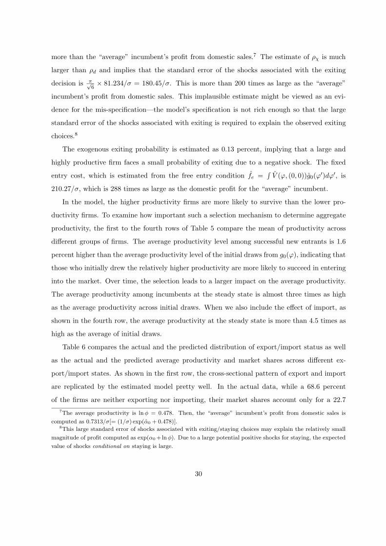
more than the “average” incumbent’s profit from domestic sales.7 The estimate of ρχ is much
larger than ρd and implies that the standard error of the shocks associated with the exiting
decision is π√6× 81.234/σ = 180.45/σ. This is more than 200 times as large as the “average”
incumbent’s profit from domestic sales. This implausible estimate might be viewed as an evi-
dence for the mis-specification—the model’s specification is not rich enough so that the large
standard error of the shocks associated with exiting is required to explain the observed exiting
choices.8
The exogenous exiting probability is estimated as 0.13 percent, implying that a large and
highly productive firm faces a small probability of exiting due to a negative shock. The fixed
entry cost, which is estimated from the free entry condition fe =∫
V (ϕ, (0, 0))g0(ϕ′)dϕ′, is
210.27/σ, which is 288 times as large as the domestic profit for the “average” incumbent.
In the model, the higher productivity firms are more likely to survive than the lower pro-
ductivity firms. To examine how important such a selection mechanism to determine aggregate
productivity, the first to the fourth rows of Table 5 compare the mean of productivity across
different groups of firms. The average productivity level among successful new entrants is 1.6
percent higher than the average productivity level of the initial draws from g0(ϕ), indicating that
those who initially drew the relatively higher productivity are more likely to succeed in entering
into the market. Over time, the selection leads to a larger impact on the average productivity.
The average productivity among incumbents at the steady state is almost three times as high
as the average productivity across initial draws. When we also include the effect of import, as
shown in the fourth row, the average productivity at the steady state is more than 4.5 times as
high as the average of initial draws.
Table 6 compares the actual and the predicted distribution of export/import status as well
as the actual and the predicted average productivity and market shares across different ex-
port/import states. As shown in the first row, the cross-sectional pattern of export and import
are replicated by the estimated model pretty well. In the actual data, while a 68.6 percent
of the firms are neither exporting nor importing, their market shares account only for a 22.77The average productivity is ln φ = 0.478. Then, the “average” incumbent’s profit from domestic sales is
computed as 0.7313/σ[= (1/σ) exp(α0 + 0.478)].8This large standard error of shocks associated with exiting/staying choices may explain the relatively small
magnitude of profit computed as exp(α0 +ln φ). Due to a large potential positive shocks for staying, the expected
value of shocks conditional on staying is large.
30

Table 4: Maximum Likelihood Estimates
Parameters Estimatesα0 -0.791 (0.004)αm 0.064 (0.002)αx -2.723 (0.025)σ0 1.090 (0.002)σf 4.382 (0.228)σfx 1.049 (0.029)σfm 0.892 (0.023)ζf 0.694 (0.004)σρd 0.462 (0.012)σρχ 81.234 (2.159)σh 0.341 (0.001)σf 1.914 (0.013)ρ 0.012 (0.001)αt 0.038 (0.001)ξ 0.0013 (0.0001)fe 210.274
log-likelihood -79389.21No. of Plants 7234
Notes: Standard errors are in parentheses. The parameters are evaluated in the unit of million US dollars in 1990.
Table 5: The Mean of Productivity
Mean of ϕ at Entry Trial 1.000
Mean of ϕ at Successful Entry 1.016Mean of ϕ at Steady State 2.948Mean of exp(αmdm)ϕ at Steady State 4.508
Notes: The reported numbers are relative to the productivity level at entry. In particular, the original numbers are divided
by the mean of ϕ at entry (i.e.,∫
ϕg0(ϕ)dϕ).
31

Table 6: Productivity and Market Shares by Export/Import Status (Actual vs. Predicted)
Export/Import Status
(1) No-Export (2) Export (3) No-Export (4) Export (2)+(4) (3)+(4)
Actual /No-Import /No-Import /Import /Import Export Import
Dist. of Ex/Im Status 0.686 0.086 0.120 0.108 0.194 0.228
Average of ln ϕ 0.035 1.532 1.434 2.596 2.118 1.978
Market Share 0.227 0.187 0.145 0.441 0.628 0.586
Predicted
Dist. of Ex/Im Status 0.678 0.090 0.126 0.106 0.196 0.232
Average of ln ϕ 0.188 0.674 0.680 2.176 1.501 1.380
Market Share 0.066 0.156 0.158 0.620 0.776 0.777
percent of total outputs. On the other hand, only a 10.8 percent of the firms are both exporting
and importing but they account for 44.1 percent of total output. The estimated model qual-
itatively replicates this pattern but the predicted magnitude of the market share is bit away
from the actual magnitude: the model under-predicts the market share for the firms that are
neither exporting nor importing while it over-predicts the market share for the exporting and
importing firms. As the actual data suggests (in the second row), relatively small number of
exporters and importers account for large market shares because they tend to be more produc-
tive and hence employ more workers relative to non-exporters and non-importers. This basic
observed pattern on the productivity across different export and import status is also captured
by the estimated model although the estimated model over-predicts the average productivity
among non-exporters and non-importers while it under-predicts the average productivity among
exporters and importers.
Table 7 compares the actual and the predicted transition probability of export/import status
and entry/exit together. Here, the estimated model fails to replicate the actual transition
pattern of export and import; in particular, the estimated model does not capture the observed
persistence in export/import status which is the prominent feature of the actual transition
probability of export/improt status. What are the missing elements from the current model
that may explain the persistence in export/import status? There are, at least, two possible
extensions. First, the current model does not incorporate the sunk start-up cost of exporting
as well as importing.9 The model with the sunk start-up cost for exporting and importing9See Roberts and Tybout (1997) for the empirical evidence for sunk start-up cost for exporting. Kasahara and
Rodrigue (2005) provides the evidence for sunk start-up cost for importing.
32

Table 7: Distribution of Export/Import Status and Entry/Exit (Actual vs. Predicted)
(1) No-Export (2) Export (3) No-Export (4) Export (2)+(4) (3)+(4) Exit at
Actual /No-Import /No-Import /Import /Import Export Import t + 1a
No-Export/No-Import at t 0.927 0.024 0.042 0.007 0.031 0.048 0.082
Export/No-Import at t 0.147 0.677 0.013 0.163 0.841 0.176 0.070
No-Export/Import at t 0.188 0.017 0.699 0.096 0.113 0.795 0.035
Export/Import at t 0.025 0.101 0.070 0.804 0.905 0.874 0.022
Predicted
No-Export/No-Import at t 0.722 0.088 0.124 0.066 0.154 0.189 0.075
Export/No-Import at t 0.660 0.093 0.131 0.116 0.209 0.247 0.066
No-Export/Import at t 0.659 0.093 0.131 0.116 0.210 0.248 0.066
Export/Import at t 0.402 0.095 0.134 0.369 0.464 0.503 0.035
Note: a). “Exit at t + 1” is defined as plants that are observed at t but not observed at t + 1 in the sample. b). “New
Entrants t” is defined as plants that are not observed at t− 1 but observed at t in the sample, of which row represents the
empirical distribution of export/import status at t as well as the probability of not being observed (i.e., exit) at t + 1.
may replicate the observed persistence in export/import status. Second, the current model only
incorporates the heterogeneity in terms of productivity while, in reality, there are other sources
of heterogeneity; some firms are inherently more likely to export or import even after controlling
for productivity. For instance, the transportation cost (τ) might be different, depending on what
kinds of products a firm is exporting. Ignoring heterogeneity other than productivity may be the
reasons for the model’s inability to capture the observed persistence of export/import status.
In the later sections, we estimate the models that incorporate sunk costs and/or other sources
of unobserved heterogeneity.
5.3 Counterfactual Experiments
While some of the structural parameters are not identified from the empirical model (crucially,
we cannot identify σ), we may solve for the change in the equilibrium aggregate price as a result
of counterfactual experiments as follows.
Denote the equilibrium aggregate price under the parameter θ by P (θ). Under the estimated
parameter θ, we may compute the estimate of fixed entry cost as: fe =∫
V (ϕ′; θ)gϕ(ϕ′; θ)dϕ′,
where V (ϕ; θ) is the fixed point of the Bellman’s equation (54) under the parameter θ and
gϕ(ϕ; θ) is the probability density function of the initial productivity under θ.
Suppose that we are interested in a counterfactual experiment characterized by a counter-
factual parameter θ that is different from the estimated parameter θ. Note that the following
33

relationships hold between α0 and the aggregate price P :
α0 = ln[αα(1− α)1−αRP (θ)σ−1]
Then, we may write the estimated profit function, (53), evaluated at the counterfactual aggregate
price P (θ) as:
π(ϕi, dit; P (θ))
=1σ
exp[(σ − 1) ln(P (θ)/P (θ))][1 + exp(αx)dxit] exp(α0 + αmdm
it + ln ϕi),
=1σ
exp[ln(K(θ)/K(θ))][1 + exp(αx)dxit] exp(α0 + αmdm
it + lnϕi),
where K(θ) = RP (θ)σ−1 is the demand shifter under the parameter θ.
Then, we may compute the equilibrium price changes in the demand shifters, ln(K(θ)/K(θ)) =
(σ − 1) ln(P (θ)/P (θ)). Specifically, the equilibrium price under the counterfactual parameter θ
is determined by the free entry condition:
fe =∫
V (ϕ′; θ, P (θ))gϕ(ϕ′; θ)dϕ′,
where the dependence of the value function V on the aggregate price P (θ) is explicitly indicated.
We may quantify the impact of counterfactual experiments on the welfare level by exam-
ining how much the equilibrium aggregate price level P changes as a result of counterfactual
experiments since the aggregate price level P is inversely related to the welfare level W .10
To quantitatively investigate the impact of international trade, we conduct the four coun-
terfactual experiments with the following counterfactual parameters:
(1) No Export: fx →∞ and αx → −∞.
(2) No Import: fm →∞ and αm = 0.
(3) Autarky: fx, fm →∞, αx → −∞, and αm = 0.
(4) No Complementarity: ζf = 1.
Table 8 presents the results of counterfactual experiments using the estimated model. To
examine the importance of equilibrium response to quantify the impact of counterfactual policies,10To see this, note that the income is constant at the level of L. From the budget constraint PQ = L and the
definition of aggregate product W = Q =[∫
ω∈Ωq(ω)ρdω
]1/ρ, the utility level is equal to W = P−1L.
34
Table 8: Counterfactual Experiments
Counterfactual Experiments
(1) (2) (3) (4)
Trade No Export No Import Autarky No Comp.
With Equilibrium Price Effect
∆(σ − 1) ln P 0.000 0.064 0.079 0.123 0.018
Exiting Rates at Entry Trial (%) 7.823 7.841 7.847 7.861 7.827
ln(Average ϕ) at Steady State 0.000 -0.026 -0.029 -0.051 -0.003
A Fraction of Exporters 0.196 0.000 0.151 0.000 0.147
A Fraction of Importers 0.232 0.191 0.000 0.000 0.188
Market Shares of Exporters 0.552 0.000 0.423 0.000 0.425
Market Shares of Importers 0.592 0.482 0.000 0.000 0.486
Without Equilibrium Price Effect
Exiting Rates at Entry Trial (%) 7.823 7.889 7.907 7.956 7.840
ln(Average ϕ) at Steady State 0.000 -0.005 -0.002 -0.011 0.003
A Fraction of Exporters 0.196 0.000 0.142 0.000 0.144
A Fraction of Importers 0.232 0.183 0.000 0.000 0.185
Market Shares of Exporters 0.552 0.000 0.407 0.000 0.422
Market Shares of Importers 0.592 0.469 0.000 0.000 0.482
Note: “Average ϕ” at Steady State is a productivity average using the plants’ combined revenues (or market shares) as
weights:∫ ∑
dϕσ−1 r(ϕ,d)P (d|ϕ)∫ ∑
d′ r(ϕ′)P (d′|ϕ′)dµ(ϕ′)dµ(ϕ).
the results both with and without equilibrium aggregate price response are reported. According
to the experiment, moving from autarky to trade may decrease the equilibrium aggregate price
by a 12.3/(σ − 1) percent. This implies that, say if σ = 4, exposure to trade increases the
real income by a (12.3/4=)3.1 percent, leading to a substantial increase in welfare. When a
country opens up its economy, more productive firms start exporting and importing, which in
turn increases the aggregate labor demand and hence leads to an increase in the real wage or a
decrease in the aggregate final goods price.
Under no equilibrium response, the exiting rates at entry trial increase from 7.82 to 7.96
percent by moving from trade to autarky; without equilibrium price response, the expected
profit is lower in autarky than in trade because there is no opportunity to export/import,
leading to higher exit rates in autarky than in trade. The equilibrium price adjustment, at least
partly, offsets this effect as we see by comparing the exiting rates in autarky between “With
Equilibrium Price Effect” and “With Equilibrium Price Effect.” When the economy moves from
trade to autarky, an increase in the equilibrium aggregate price increases the expected profit
increases, which in turn lowers the exiting rates from 7.96 to 7.86.
The impact of trade on aggregate productivity—measured by a productivity average us-
35
ing the plants’ market shares as weights—can be understood by comparing “ln(Average ϕ) at
Steady State” between trade and autarky. Moving from trade to autarky leads to a 5.1 decrease
in aggregate productivity at the steady state. Here, by comparing between with and without the
equilibrium price responses, we notice the importance of equilibrium price response to quantita-
tively explain the impact of trade on aggregate productivity; without equilibrium price response,
the impact of trade on aggregate productivity is only 1.1 percent as opposed to 5.1 percent.
The counterfactual experiments under no export or no import (but not both) highlight the
interaction between aggregate export and aggregate import in the presence of heterogenous
firms. According to the estimated model, when the economy moves from trade to no import, a
fraction of exporters declines from a 19.6 percent to a 15.1 percent; when the economy moves
from trade to no export, a fraction of importers declines from a 23.2 percent to a 19.1 percent.
In terms of market shares, moving from trade to no import leads to a decrease in the total
market shares of exporters from 55.2 to 42.3 percent while moving from trade to no export leads
to a decrease in the total market shares of importers from 59.2 to 48.2 percent. Thus, policies
that prohibits the import of foreign materials could have a large negative impact on the export
of final consumption goods, or vice-versa. The similar results hold even without equilibrium
price effect and thus the equilibrium price response is little to do with these results. Rather,
it is due to the complementarity between export and import within both revenue function r(·)and sunk-cost function F (·).
To examine the role of complementarity between export and import in the sunk-cost function—
relative to the role played by the complementarity in the revenue function—we conducted what
would happen to a fraction of importers and/or a fraction of exporters had there been no com-
plementarity between export and import in the sunk cost function. The results are striking.
Eliminating the complementarity between export and import in the sunk cost function has es-
sentially the same effect on export and import, respectively, as restricting to no import and
no export. Thus, the results from the experiments show that it is the complementarity in the
sunk cost function, rather than the complementarity in the revenue function, that determines
the impact of exporting policies (e.g., export subsidies) on intermediate imports or the impact
of importing policies (e.g., import tariffs) on exports.
36

6 The Dynamic Model
6.1 The Environment
In this section, we modify the above environment to introduce interesting dynamics into the
model to facilitate structural estimation of the model in the next section. Preferences and pro-
duction technologies are unchanged but we modify the processes governing productivity. Firms
continue to pay a fixed cost of entry and a fixed per-period production cost but we modify the
fixed costs associated with exporting and importing. We begin with a description of productivity
draws. Upon entering, an entrant draws an initial productivity from a continuous cumulative
distribution G0(·) and the density function g0(·). After the initial realization, productivity at
time t, ϕt, follows a first-order Markov process, where the distribution of ϕt+1 conditional on ϕt
is given by G(·|ϕt) with density function g(·|ϕt).
There are both per-period fixed costs and one-time sunk costs associated with exporting and
importing:
F (dt, dt−1) = f + ζdx
t dmt
f (fxdxt + fmdm
t ) + ζdx
t dmt
c [ζdm
t−1cx cxdx
t (1− dxt−1) + ζ
dxt−1
cm cmdmT (1− dm
t−1)].
The second term on the right hand side, ζdx
t dmt
f (fxdxt + fmdm
t ), captures per-period fixed cost
while the third term, ζdx
t dmt
c (ζdm
t−1cx cxdx
t (1− dxt−1) + ζ
dxt−1
cm cmdmt (1− dm
t−1)), captures one-time sunk
cost associated with exporting and importing. The parameter 0 < ζf < 1 determines the degree
of complementarity between current export and import in per-period fixed cost. Similarly, the
parameter 0 < ζc < 1 captures the degree of complementarity between current export and import
in one-time sunk cost. While the parameter 0 < ζcx < 1 captures the dynamic effect of past
import status on the current sunk cost of exporting, 0 < ζcm < 1 captures the dynamic effect
of past export status on the current sunk cost of importing. If ζcx < 1, then the past importing
experience reduces the one-time sunk cost of exporting and hence increases the probability of
exporting this period.
A firm’s net profit depends on the current productivity ϕT and current and past export/import
status (dT , dt−1):
π(ϕt, dt, dt−1) =r(ϕt, dt)
σ− F (dt, dt−1).
Denote the exiting decision by χ ∈ 0, 1 where χT = 1 indicates that a firm is operating at
t and χT = 0 implies that a firm exits at the beginning of period t.
37

There are choice-dependent idiosyncratic cost shocks associated with exiting decisions as
well as export/import decisions. If a firm chooses χt ∈ 0, 1, then it has to pay the additional
cost of εχt (χt) associated with the exiting choice χT , where εχ = (εχ(0), εχ(1)) is drawn from
the cumulative distribution Hχ(·). Similarly, if a firm chooses dt = (dxt , dm
t ) ∈ 0, 12 this
period, then it has to pay εdt (dt), where εd = (εd(0, 0), εd(1, 0), εd(0, 1), εd(1, 1)) is drawn from
the cumulative distribution Hd(·).The discount factor is given by β ∈ (0, 1). The timing of the incumbent’s decision with the
state (ϕt−1, dt−1) within each period is as follows. At the beginning of every period, a firm faces
a possibility of a large negative shock that leads it to exit with an exogenous probability ξ. If the
firm survives, it draws ϕt from the cumulative distribution G(·|ϕt−1) and the additional choice-
dependent idiosyncratic cost shocks associated with exiting decisions, εχT = (εχ
T (0), εχT (1)), from
Hχ(·). Given the realizations, the firm decides whether it exits from the market or continues to
operate. If the firm decides to exit, it receives the terminal value of εχT (0). If the firm decides to
continue to operate, then it will draw the choice-dependent idiosyncratic cost shocks associated
with export and import, εdT (d) for d ∈ 0, 12. After observing εd
T (d),the firm makes export and
import decisions. The Bellman’s equation is written as:
V (ϕt, dt−1) =∫
maxεχ′(0),W (ϕt, dt−1) + εχ′(1)dHχ(εχ′)
W (ϕt, dt−1) =∫
maxdt∈0,12
W (ϕT , dT , dt−1) + εd′(dt)
dHd(εd′), (45)
where
W (ϕT , dT , dt−1) = π(ϕt, dt, dt−1) + β(1− ξ)∫
V (ϕ′, dt)G(dϕ′|ϕt).
The policy function associated with this Bellman’s equation (45), together with the exogenous
process of ϕt, determines the transition function of (ϕt, dt). For a firm with the state (ϕt, dt−1),
the exiting probability is:
P (χt = 0|ϕt, dt−1) = ξ + (1− ξ)∫
1(εχ′(0) > W (ϕt, dt−1) + εχ′(1))dHχ(εχ′), (46)
where χit ∈ 0, 1 represents the exiting/staying decision. The probability of choosing dit = (i, j)
for (i, j) ∈ 0, 12 conditional on the survival is
P (dt = (i, j)|ϕt, dt−1, χt = 1) =∫
1[(i, j) = argmaxdT∈0,12
W (ϕT , dT , dt−1) + εd′(dt)
]dHd(εd′).
(47)
38
6.2 Stationary Equilibrium
As before, we focus on a stationary equilibrium in which the joint distribution of (ϕ, d) is constant
over time and let the stationary distribution of (ϕ, d) among incumbents is denoted by µ(ϕ, d).
Equations (??)-(??) continue to hold in this dynamic economy.
New entrants are assumed to have no past export/import experience so that dt−1 = (0, 0).
The probability of successful entry among new entrants is pin =∫
P (χt = 1|ϕ′, dt−1 = (0, 0))dG0(ϕ′).
The expected value of an entering firm is given by∫
V (ϕ′, dT = (0, 0))dG0(ϕ′), where V (·) is
given in (45). Under free entry, this value must be equal to the fixed entry cost fe:
∫V (ϕ′, dT = (0, 0))dG0(ϕ′) = fe. (48)
In equilibrium, this free entry condition has to be satisfied.
Given the stationary distribution, the average probability of exiting among incumbent is
δ =∫
P (χt = 0|ϕ′, d′)dµ(ϕ′, d′). The stationarity requires that the number of exiting firms is
equal to the number of successful new entrants:
δM = pinMe,
where Me is the mass of new entrants.
The evolution of the probability measure among incumbents has to take account of both the
transition of states among survivors and entry/exit processes. Define the probability that a firm
with the state (ϕt−1, dt−1) continues in operation at t with the state (ϕt, dt) is
P (ϕt, dt, χT = 1|ϕt−1, dt−1) = P (dt|ϕt, dt−1, χt = 1)P (χt = 1|ϕt, dt−1)g(ϕT |ϕt−1).
The probability that a new successful entrant will operate with the state (ϕt, dt) is:
Pe(ϕT , dT ) = P (dt|ϕt, dt−1 = (0, 0), χT = 1)g0(ϕt). (49)
Again, new entrants have no past export/import experience so that dt−1 = (0, 0) because they
have no past export/import experience.
Then, the transition of the measure µ(ϕ, d) is determined by:
µt(ϕ, d) = (Tµt−1)(ϕ, d) ≡∫
P (ϕ, d, χ = 1|ϕ′, d′)dµt−1(ϕ′, d′) + δPe(ϕ, d). (50)
39

Here, we impose the equilibrium condition that the mass of entrants is equal to the mass of exits
so that δPe(ϕ, d) represents the probability measure of new entrants with the state (ϕ, d).11 The
stationary distribution, µ, is a fixed point of the operator T : µ = Tµ.
A stationary equilibrium consists of an aggregate price P , an aggregate revenue R, a mass
of incumbents M , and a probability distribution of incumbents µ such that
• Given the the aggregates P and R (and hence the demand function (??)), a firm solves
the Bellman equation (45).
• Free Entry condition (48) holds.
• The probability distribution µ is a fixed point of the operator T induced by a firm’s policy
function: T (µ) = µ.
• The mass of incumbents is a constant over time: δM = pinMe.
• Aggregate budget constraint holds: R = L.12
6.3 Algorithm for Computing a Stationary Equilibrium
Define the demand shifter K ≡ RP σ−1 (See the demand function (??)).
1. For fixed value of K = Kj , we may compute the revenue function r and solve the Bellman
equation (45) and obtain the choice probabilities, (46)-(47).
2. Compute J(Kj) = (∫
V (ϕ′, (0, 0))dG0(ϕ′)− fe)2.
3. Repeat Step 1-2 to find K∗ such that J(K∗) = 0.
4. Using (46)-(47), compute a stationary distribution µ by computing a fixed point of the
operator T .11Denote the mass of incumbents at t by MT . The mass of incumbents with the state (ϕt−1, dt−1) at t − 1
is Mt−1µt−1(ϕt−1, dt−1). Among them, the mass P (χT = 0|ϕt−1, dt−1)Mt−1µt−1(ϕt−1, dt−1) exits from the
market, and only the mass of P (ϕT , dt, χt = 1|ϕt−1, dt−1)Mt−1µt−1(ϕt−1, dt−1) will survive and reach the state
(ϕT , dt) at t. The mass of incumbents at t with the state (ϕT , dt) who are not new entrants can be com-
puted by summing up P (ϕT , dt, χt = 1|ϕt−1, dt−1)Mt−1µt−1(ϕt−1, dt−1) over the distribution µt−1(ϕt−1, dt−1):
Mt−1
∫P (ϕT , dt, χit = 1|ϕ′, d′)dµt−1(ϕ
′, d′). On the other hand, the mass of successful new entrants with the
state (ϕT , dt) is pinMePe(ϕT , dT ). Therefore, the transition of the distribution of incumbent’s state is written as
MT µt(ϕ, d) = Mt−1
∫P (ϕ, d, χ = 1|ϕ′, d′)dµt−1(ϕ
′, d′)+pinMe,tPe(ϕ, d). The stationary equilibrium requires that
(i) pinMe,t = δMt−1 and (ii) Mt−1 = Mt. Then, we get µt(ϕ, d) =∫
P (ϕ, d, χ = 1|ϕ′, d′)dµt−1(ϕ′, d′)+ δPe(ϕ, d).
12This condition implies labor market clearing.
40

5. Compute the aggregate price index as P = (K∗/R)1
σ−1 = (K∗/L)1
σ−1 .
6. Compute M from (??) as M = R∫r(ϕ′,d′)dµ(ϕ′,d′)
= L∫r(ϕ′,d′)dµ(ϕ′,d′)
.
7 Structural Estimation of Dynamic Model
7.1 Empirical Specification
Use the subscript i to represent plant i and the subscript t to represent year t. To develop an
estimable structural model, we make the following distributional assumptions:
• We assume that lnϕit follows an AR(1) process: lnϕit = ψ ln ϕit−1 + ωit, where ψ ∈ (0, 1)
and ωit is independently drawn from N(0, σ2ω). That is, g(ϕit|ϕit−1) = 1
σωφ((lnϕit −
ψ ln iit−1)/σω).
• The logarithm of the initial productivity upon entry is drawn from N(0, σ20) so that
g0(ϕit) = 1σ0
φ(lnϕit/σ0).13
• εχit(0) and εχ
it(1) are independently drawn from the identical extreme-value distribution
with mean zero and scale parameter %χ.
• εdit(d)’s for d ∈ 0, 12 are independently drawn from the identical extreme-value distribu-
tion with mean zero and scale parameter %d.
We also assume that there is an idiosyncratic shock to export revenue, denoted by ηt, inde-
pendently drawn from N(−0.5σ2η, ση) and its density function is given by gη(η) = φ(η/ση)/ση.14
For simplicity, we assume that this idiosyncratic shock is observed only after the current year’s
export decision is made so that ηit does not affect the firm’s export decision. The inclusion of
export-revenue specific shocks is necessary to deal with the feature of the data that a substantial
variation in export revenue even after controlling for domestic revenue. We also consider labor
augmented technological change at the annual rate of αt.
Modifying the revenue functions, we specify the logarithm of the domestic revenue and the
export revenue as:
ln rhit = α0 + αtt + αmdm
it + ln ϕit (51)13The mean of initial productivity draws is set to zero in order to achieve the identification. ln ϕ0 cannot be
separately identified from αh0 and αf
0 .14Assuming that the mean of η is equal to −0.5σ2
η, we get E[exp(η)] = 1.
41

ln rfit = α0 + αtt + αx + αmdm
it + ln ϕit + ηit. (52)
Importantly, they are reduced-form specifications; we have the following relationships between
reduced-form parameters and structural parameters:15
α0 = ln[αα(1− α)1−αRP σ−1],
αx = ln[Nτ1−σ],
αm = (σ − 1) ln λ.
Note that α0 crucially depends on the aggregate price P . This means that the values of α0 will
not be invariant with respect to policy changes as long as policy changes induce the equilibrium
response to the aggregate price P . When we conduct counterfactual policy experiments later,
we will pay a particular attention on the role of the equilibrium price response.
Given these specifications for revenues, firm’s profit—after detrending and taking an expec-
tation with respect to ηit—is
π(ϕit, dit, dit−1) =1σ
(1 + exp(αx)dxit) exp(α0 + αmdm
it + ln ϕit)− F (dit, dit−1). (53)
Note that, by detrending and redefining the discount factor as β = β(1 − ξ)eαt , the firm’s
dynamic optimization problem becomes stationary.
Using the properties of the extreme-value distributed random variables (See the Appendix),
the Bellman’s equation (45) is rewritten as:
V (ϕit, dit−1) = %χ ln(exp(0) + exp(W (ϕit, dit−1)/%χ))
W (ϕit, dit−1) = %d ln
∑
dit
exp(
[π(ϕit, dit, dit−1) + β
∫V (ϕ′, dit)G(dϕ′|ϕit)]/%d
) . (54)
With the solution to the functional equation (54), the conditional choice probabilities of
exiting and export/import decisions follow the Nested Logit formula. In particular, the choice
probability of exiting and staying conditional on the state (ϕit, dit−1)—which corresponds to
(46)—is given by:
P (χit|ϕit, dit−1) = (1− χit)ξ + (1− ξ)exp(χitW (ϕit, dit−1)/%χ)
exp(0) + exp(W (ϕit, dit−1)/%χ). (55)
15Also, with abuse of notation, we replace (σ− 1) ln ϕ by ln ϕ since (σ− 1) cannot be separately identified from
the variance of ln ϕ.
42

Conditional on choosing χit = 1 (i.e., continuously operating), the choice probabilities of dit,
corresponding to (47), are given by the multinomial logit formula:
P (dit|ϕit, dit−1, χit = 1) =exp([π(ϕit, dit, dit−1) + β
∫V (ϕit+1, dit)G(dϕit+1|ϕit)]/%d)
∑d′∈0,12 exp([π(ϕit, d′, dit−1) + β
∫V (ϕit+1, d′)G(dϕit+1|ϕit)]/%d)
,
(56)
To achieve the identification, we normalize the profit function by 1/σ; the various components
of the fixed cost as well as the scale parameter %d are estimated up to the scale of σ.
The probability that a new successful entrant will operate with the state (ϕt, dt), correspond-
ing to (49), is:
Pe(ϕit, dit) = P (dit|ϕit, dit−1 = (0, 0), χit = 1)P (ϕit|χit = 1), (57)
where P (dit|ϕit, dit−1 = (0, 0), χit = 1) is given in (56) and P (ϕit|χit = 1) can be computed,
using (55), as:
P (ϕit|χit = 1) =P (χit = 1|ϕit, dit−1 = (0, 0))g0(ϕit)∫P (χit = 1|ϕ′, dit−1 = (0, 0))g0(ϕ′)dϕ′
.
To obtain the transition function of the state, define the probability that a firm with the
state (ϕit−1, dit−1) continues in operation at t with the state (ϕit, dit) as:
P (ϕit, dit, χit = 1|ϕit−1, dit−1) = P (dit|ϕit, dit−1, χit = 1)P (χit = 1|ϕit, dit−1)g(ϕit|ϕit−1).
Then, the transition of the measure µ(ϕ, d) is determined by (50).
7.2 Econometric Approach
The parameter vector to be estimated is θ = (αt, α0, αx, αm, σ2ω, σ2
0, f, fx, fm, ζf , cx, cm, ζc, %χ, %d, ξ).
The discount factor β is not estimated and is set to 0.95. The parameters are estimated by the
method of Maximum Likelihood.
Given the data and the parameter vector θ, we may compute the estimates of lnϕit as:
ln ϕit(θ) = ln rhit − α0 − αtt− αmdm
it
ηit(θ) = ln rfit − α0 − αtt− αxdx
it − αmdmit − ln ϕit(θ)
Denote the first year and the last year in which firm i appears in the data by Ti,0 and Ti,1,
respectively. The unbalanced plant-level data spans from 1990 to 1996. Thus, Ti,0 is either 1990
43

or the year in which firm i entered between 1991 and 1996. Ti,1 is either 1996 or the year in
which firm i exited between 1991 and 1995.
For t > Ti,0, we can observe the past state variables (dit−1, ϕit−1); we may compute the
likelihood contribution of the current observation (dit, ϕit, ηit) conditioned on the observable
past state variable (dit−1, ϕit−1) as
Lit(θ) =
P (χit = 1|ϕit, dit−1)P (dit|ϕit, dit−1, χit = 1)g(ϕit|ϕit−1)gη(eηit)dxit , for χit = 1
∫P (χit = 0|ϕ′, dit−1)g(ϕ′|ϕit−1)dϕ′, for χit = 0
(58)
Each of the terms is explained as follows. First, P (dit, χit = 1|ϕit, dit−1) = P (χit = 1|ϕit, dit−1)
P (dit|ϕit, dit−1, χit = 1) is the likelihood of observing (dit, χit = 1) conditioned on the current
productivity ϕit and the past export/import decision dit−1. g(ϕit|ϕit−1) is the likelihood of
observing ϕit conditioning on the past state variable. If a firm is exporting (i.e., dxit = 1), then
the likelihood of observing ηit is also computed as gη(ηit). The likelihood Lit(θ) for χit = 1 is,
therefore, the probability of observing (dit, ϕit, ηit) conditioned on the past state variables (dit−1,
ϕit−1). In the case of χit = 0 (i.e., firm i exists at t), we do not observe the current productivity
shock ϕit. So, in order to compute the probability of exiting conditioned on (dit−1, ϕit−1),
we integrate out P (χit = 0|ϕit, dit−1) over unobserved current shock ϕit using the conditional
density function g(ϕit|ϕit−1).
For t = Ti,0, there are two cases. The first case is that firm i enters into the market after
1991 (i.e., Ti,0 > 1990). The second case is that firm i has operated in 1990.
Consider the first case of Ti,0 > 1990. The likelihood of observing (dit, ϕit, ηit) for t = Ti,0 is
written as
Lit(θ) = Pe(ϕit, dit)gη(ηit)dxit , (59)
where Pe(ϕ, d) is given in equation (57). For a new successful entrant, productivity shock ϕit is
distributed according to Pe(ϕit|χit = 1), which is the distribution of initial draws conditioned
on the successful entry.
Next, consider the case of Ti,0 = 1990. While the evaluation of the choice-probabilities
(55)-(56) as well as the probability of observing ϕit requires the past state variables (dit−1,
ϕit−1), we do not observe these past state variables at t = 1990 in this case. Note, however,
that the theory suggests that the past state variables (dit−1, ϕit−1) is distributed according to
a stationary distribution of (dit−1, ϕit−1), implied by the policy function associated with the
44
parameter vector θ. Thus, we may use the stationary distribution to integrate out the unobserved
past state variables to compute the likelihood of the initial observations. The likelihood is
Lit(θ) =∫
P (χit = 1|ϕit, d′)P (dit|ϕit, d
′, χit = 1)g(ϕit|ϕ′)gη(ηit)dxitdµ(ϕ′, d′). (60)
In sum, the likelihood contribution from the observation of firm i at t is computed as
Lit(θ) =
Pe(ϕit, dit)gη(ηit)dxit for t = Ti,0 > 1990,
∫P (χit = 1|ϕit, d
′)P (dit|ϕit, d′, χit = 1)g(ϕit|ϕ′)gη(ηit)dx
itdµ(ϕ′, d′) for t = Ti,0 = 1990,
P (χit = 1|ϕit, dit−1)P (dit|ϕit, dit−1, χit = 1)g(ϕit|ϕit−1)gη(eηit)dxit , for χit = 1 and t > Ti,0,
∫P (χit = 0|ϕ′, dit−1)g(ϕ′|ϕit−1)dϕ′ for χit = 0 and t > Ti,0.
The parameter vector θ can be estimated by maximizing the logarithm of likelihood function
L(θ) =N∑
i=1
Ti,1∑
t=Ti,0
ln Lit(θ). (61)
Evaluation of the log-likelihood involves solving computationally intensive dynamic program-
ming problem that approximates the Bellman equation (54) by discretization of state space. For
each candidate parameter vector θ, we solve the discretized version of (54) and then obtain the
choice probabilities, (55) and (56), as well as the stationary distribution from the associated
policy function. Once the choice probabilities and the stationary distribution are obtained for a
particular candidate parameter vector θ, then we may evaluate the log-likelihood function (61).
Repeating this process, we can maximize (61) over the parameter vector space of θ to find the
estimate.
In practice, we use the Gauss-Hermit quadrature grids to discretize the space of ϕ so that
the integral in (54) can be approximately evaluated using the Hermit quadrature formula (c.f.,
Tauchen and Hussey, 1991; Stinebrickner, 2000). Another important issue is that, while the con-
ditional choice probabilities, (55) and (56), can be evaluated only on the set of finite quadrature
grids, we need to evaluate the conditional choice probabilities on the realized value of ϕit which
is not necessarily on the set of grid points. We evaluate the conditional choice probabilities (55)
and (56) at ϕit that is not on the quadrature grids by using cubic spline interpolation. The
appendix discusses the approximation method in greater detail. To maximize the log-likelihood
function (61), we first use the simplex method of Nelder and Mead to reach the neighborhood
of the optimum and then use the BFGS quasi-Newton method.
45
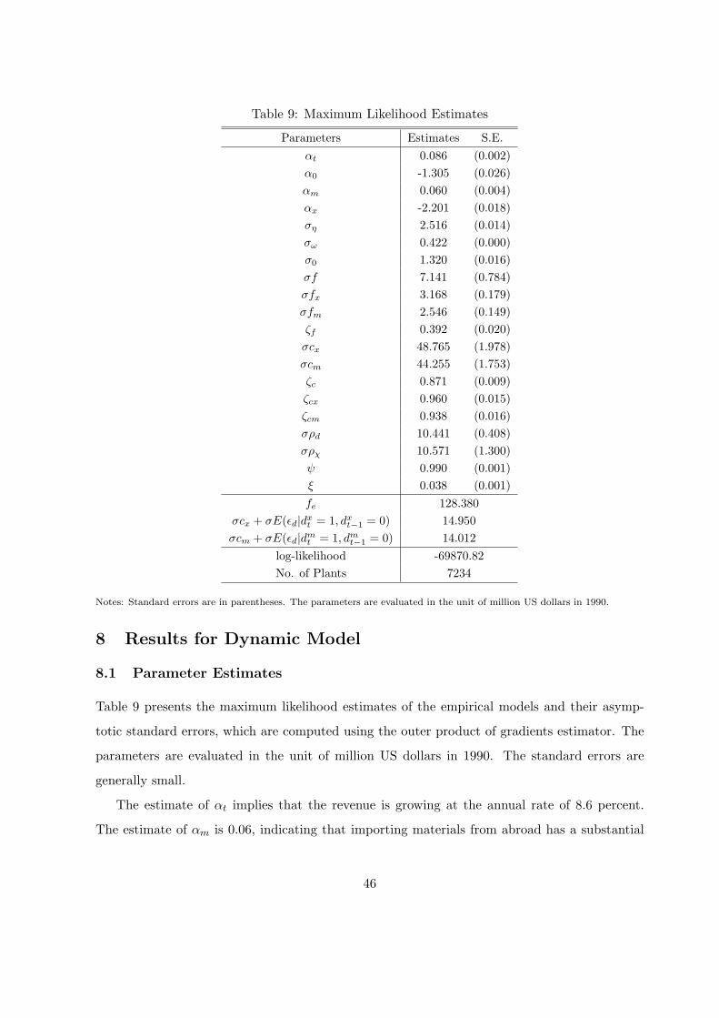
Table 9: Maximum Likelihood Estimates
Parameters Estimates S.E.αt 0.086 (0.002)α0 -1.305 (0.026)αm 0.060 (0.004)αx -2.201 (0.018)ση 2.516 (0.014)σω 0.422 (0.000)σ0 1.320 (0.016)σf 7.141 (0.784)σfx 3.168 (0.179)σfm 2.546 (0.149)ζf 0.392 (0.020)σcx 48.765 (1.978)σcm 44.255 (1.753)ζc 0.871 (0.009)ζcx 0.960 (0.015)ζcm 0.938 (0.016)σρd 10.441 (0.408)σρχ 10.571 (1.300)ψ 0.990 (0.001)ξ 0.038 (0.001)fe 128.380
σcx + σE(εd|dxt = 1, dx
t−1 = 0) 14.950σcm + σE(εd|dm
t = 1, dmt−1 = 0) 14.012
log-likelihood -69870.82No. of Plants 7234
Notes: Standard errors are in parentheses. The parameters are evaluated in the unit of million US dollars in 1990.
8 Results for Dynamic Model
8.1 Parameter Estimates
Table 9 presents the maximum likelihood estimates of the empirical models and their asymp-
totic standard errors, which are computed using the outer product of gradients estimator. The
parameters are evaluated in the unit of million US dollars in 1990. The standard errors are
generally small.
The estimate of αt implies that the revenue is growing at the annual rate of 8.6 percent.
The estimate of αm is 0.06, indicating that importing materials from abroad has a substantial
46

impact, a 6.0 percent increase, on the total revenues. The standard error for export revenue is
estimated as 2.51, which seems to be high. This high estimate might be due to our specification
for export revenue function.16
The estimated per-period fixed cost of operating in the market is f = 7.14/σ million dollars.
Thus, if, say, σ = 4, the estimated per-period fixed cost is approximately equal to 1.8 million US
dollars. On the other hand, this per-period fixed cost is more than eight times as large as the
profit from domestic sales for the “average” incumbent with the average productivity lnϕ = 1.09,
(exp(α0 + 1.09)/σ =)0.81/σ. Taken for face value, the result indicates that many firms put up
with the profit loss for a potential big success in the future—a possible realization of a high
value of ϕ. The estimated per-period fixed costs for export and import are also substantial:
fx = 3.17/σ and fm = 2.55/σ. The parameter determining the degree of complementarity in
the per-period fixed cost associated with export and import, ζf , is estimated as 0.392, indicating
that a firm can save more than a half of per-period fixed cost associated with trade by engaging
in both export and import activities.
The estimated one-time sunk costs associated with export and import are also large: cx =
48.77/σ and cm = 44.26/σ. We have to be careful, however, in interpreting these numbers since
a firm is also getting a random shock ε(d). Since a firm tends to start exporting when a firm
draws a lower random shock εd(dx = 1), the average value of εd a firm is paying is low and tends
to be negative. If we take into account the random shock, the average sunk cost paid among the
firms that start exporting (or importing) is computed as cx + E(εd(dxt = 1)|dx
t = 1, dxt−1 = 0) =
14.95/σ (or cm + E(εd(dmt = 1)|dm
t = 1, dmt−1 = 0) = 14.01/σ), which is substantially lower than
cx = 48.77/σ (or cm44.26/σ). This means that, on average, a firm pays the sunk start-up cost
of exporting (importing) that is about 18 (14) times as large as the average incumbent’s annual
profit from domestic sales.
The parameter estimate ζc = 0.871 indicates that a firm can save more than 12 percent
of one-time sunk cost for export and import if it simultaneously exports and imports. On the
other hand, ζcx = 0.960 and ζcm = 0.938 imply that the past import experience reduces the
sunk cost for exporting by 4.0 percent while the past export experience reduces the sunk cost
for importing by 6.2 percent.
The estimated magnitudes of the shocks associated with the exiting decision and the ex-16The current specification might not be rich enough to capture the process of export revenue shocks.
47
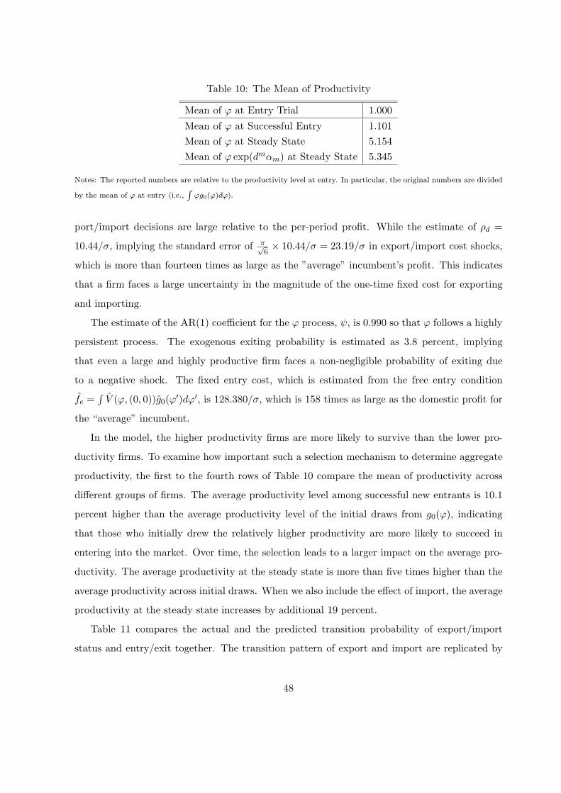
Table 10: The Mean of Productivity
Mean of ϕ at Entry Trial 1.000
Mean of ϕ at Successful Entry 1.101Mean of ϕ at Steady State 5.154Mean of ϕ exp(dmαm) at Steady State 5.345
Notes: The reported numbers are relative to the productivity level at entry. In particular, the original numbers are divided
by the mean of ϕ at entry (i.e.,∫
ϕg0(ϕ)dϕ).
port/import decisions are large relative to the per-period profit. While the estimate of ρd =
10.44/σ, implying the standard error of π√6× 10.44/σ = 23.19/σ in export/import cost shocks,
which is more than fourteen times as large as the ”average” incumbent’s profit. This indicates
that a firm faces a large uncertainty in the magnitude of the one-time fixed cost for exporting
and importing.
The estimate of the AR(1) coefficient for the ϕ process, ψ, is 0.990 so that ϕ follows a highly
persistent process. The exogenous exiting probability is estimated as 3.8 percent, implying
that even a large and highly productive firm faces a non-negligible probability of exiting due
to a negative shock. The fixed entry cost, which is estimated from the free entry condition
fe =∫
V (ϕ, (0, 0))g0(ϕ′)dϕ′, is 128.380/σ, which is 158 times as large as the domestic profit for
the “average” incumbent.
In the model, the higher productivity firms are more likely to survive than the lower pro-
ductivity firms. To examine how important such a selection mechanism to determine aggregate
productivity, the first to the fourth rows of Table 10 compare the mean of productivity across
different groups of firms. The average productivity level among successful new entrants is 10.1
percent higher than the average productivity level of the initial draws from g0(ϕ), indicating
that those who initially drew the relatively higher productivity are more likely to succeed in
entering into the market. Over time, the selection leads to a larger impact on the average pro-
ductivity. The average productivity at the steady state is more than five times higher than the
average productivity across initial draws. When we also include the effect of import, the average
productivity at the steady state increases by additional 19 percent.
Table 11 compares the actual and the predicted transition probability of export/import
status and entry/exit together. The transition pattern of export and import are replicated by
48
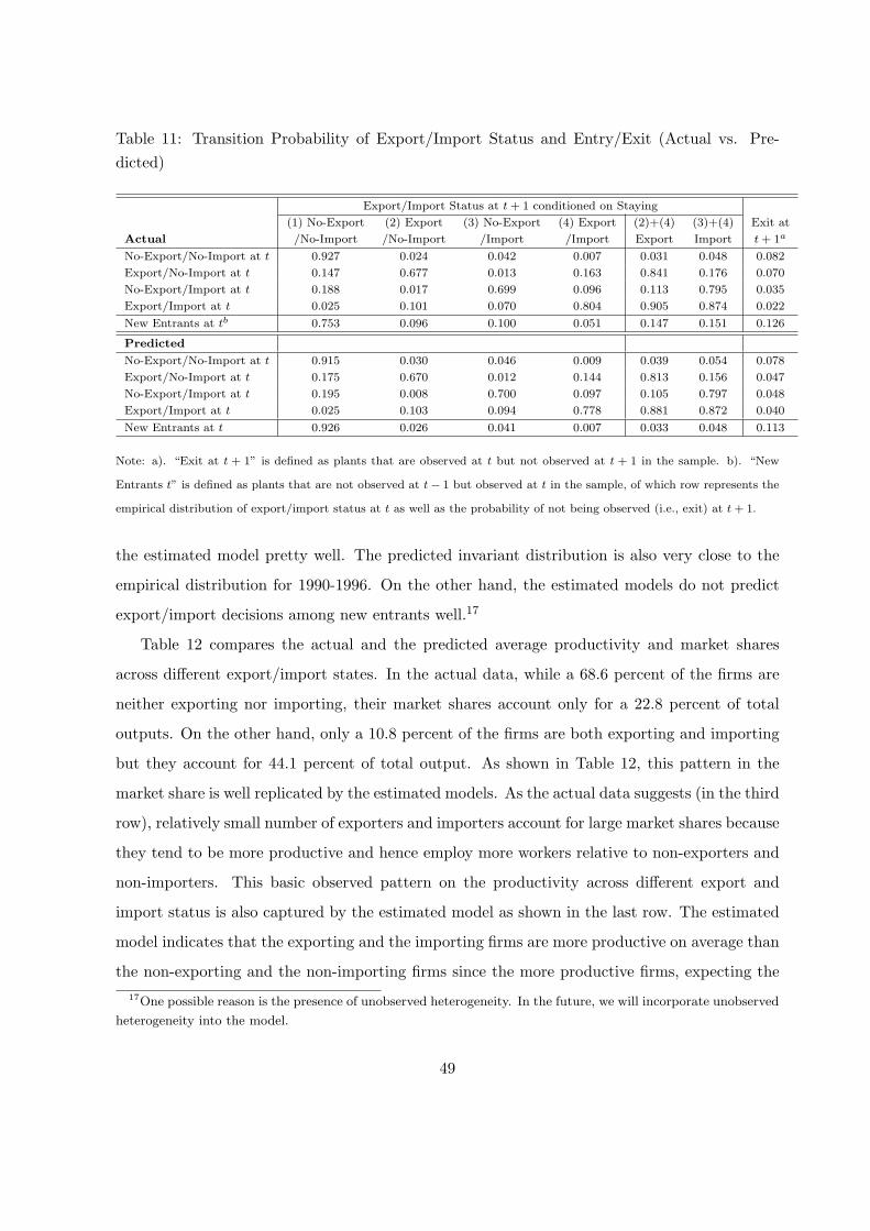
Table 11: Transition Probability of Export/Import Status and Entry/Exit (Actual vs. Pre-dicted)
Export/Import Status at t + 1 conditioned on Staying
(1) No-Export (2) Export (3) No-Export (4) Export (2)+(4) (3)+(4) Exit at
Actual /No-Import /No-Import /Import /Import Export Import t + 1a
No-Export/No-Import at t 0.927 0.024 0.042 0.007 0.031 0.048 0.082
Export/No-Import at t 0.147 0.677 0.013 0.163 0.841 0.176 0.070
No-Export/Import at t 0.188 0.017 0.699 0.096 0.113 0.795 0.035
Export/Import at t 0.025 0.101 0.070 0.804 0.905 0.874 0.022
New Entrants at tb 0.753 0.096 0.100 0.051 0.147 0.151 0.126
Predicted
No-Export/No-Import at t 0.915 0.030 0.046 0.009 0.039 0.054 0.078
Export/No-Import at t 0.175 0.670 0.012 0.144 0.813 0.156 0.047
No-Export/Import at t 0.195 0.008 0.700 0.097 0.105 0.797 0.048
Export/Import at t 0.025 0.103 0.094 0.778 0.881 0.872 0.040
New Entrants at t 0.926 0.026 0.041 0.007 0.033 0.048 0.113
Note: a). “Exit at t + 1” is defined as plants that are observed at t but not observed at t + 1 in the sample. b). “New
Entrants t” is defined as plants that are not observed at t− 1 but observed at t in the sample, of which row represents the
empirical distribution of export/import status at t as well as the probability of not being observed (i.e., exit) at t + 1.
the estimated model pretty well. The predicted invariant distribution is also very close to the
empirical distribution for 1990-1996. On the other hand, the estimated models do not predict
export/import decisions among new entrants well.17
Table 12 compares the actual and the predicted average productivity and market shares
across different export/import states. In the actual data, while a 68.6 percent of the firms are
neither exporting nor importing, their market shares account only for a 22.8 percent of total
outputs. On the other hand, only a 10.8 percent of the firms are both exporting and importing
but they account for 44.1 percent of total output. As shown in Table 12, this pattern in the
market share is well replicated by the estimated models. As the actual data suggests (in the third
row), relatively small number of exporters and importers account for large market shares because
they tend to be more productive and hence employ more workers relative to non-exporters and
non-importers. This basic observed pattern on the productivity across different export and
import status is also captured by the estimated model as shown in the last row. The estimated
model indicates that the exporting and the importing firms are more productive on average than
the non-exporting and the non-importing firms since the more productive firms, expecting the17One possible reason is the presence of unobserved heterogeneity. In the future, we will incorporate unobserved
heterogeneity into the model.
49

Table 12: Productivity and Market Shares by Export/Import Status (Actual vs. Predicted)
Export/Import Status
(1) No-Export (2) Export (3) No-Export (4) Export (2)+(4) (3)+(4)
/No-Import /No-Import /Import /Import Export Import
Actual Dist. of Ex/Im Status 0.686 0.086 0.120 0.108 0.194 0.228
Market Shares 0.228 0.187 0.145 0.441 0.627 0.586
Average of ln ϕ 0.484 1.337 1.474 2.381 1.911 1.898
Predicted Dist. of Ex/Im Status 0.659 0.092 0.128 0.121 0.213 0.249
Market Shares 0.254 0.118 0.101 0.527 0.645 0.628
Average of ln ϕ 0.763 1.507 1.262 2.349 1.984 1.789
higher returns from exporting and importing, are more willing to pay the one-time fixed costs
of exporting and importing and hence are more likely to become exporters and importers.
8.2 Counterfactual Experiments
While some of the structural parameters are not identified from the empirical model (crucially,
we cannot identify σ), we may solve for the change in the equilibrium aggregate price as a result
of counterfactual experiments as follows.
Denote the equilibrium aggregate price under the parameter θ by P (θ). Under the estimated
parameter θ, we may compute the estimate of fixed entry cost as: fe =∫
V (ϕ′, (0, 0); θ)g0(ϕ′; θ)dϕ′,
where V (ϕ, d; θ) is the fixed point of the Bellman’s equation (54) under the parameter θ and
g0(ϕ; θ) is the probability density function of the initial productivity under θ.
Suppose that we are interested in a counterfactual experiment characterized by a counter-
factual parameter θ that is different than the estimated parameter θ. Note that the following
relationships hold between α0 and the aggregate price P :
α0 = ln(αα(1− α)1−αRP (θ)σ−1).
Then, we may write the estimated profit function, (53), evaluated at the counterfactual aggregate
price P (θ) as:
π(ϕt, dt, dt−1;P (θ))
=1σ
exp[(σ − 1) ln(P (θ)/P (θ))](1 + exp(αx)dxt ) exp(α0 + αmdm
t + ln ϕt)− F (dt, dt−1),
=1σ
exp[ln(K(θ)/K(θ))](1 + exp(αx)dxt ) exp(α0 + αmdm
t + ln ϕt)− F (dt, dt−1),
50

where K(θ) = RP (θ)σ−1 is the demand shifter under the parameter θ.
Then, we may compute the equilibrium changes in the demand shifters, ln(K(θ)/K(θ)) =
(σ − 1) ln(P (θ)/P (θ)). Specifically, we may use the same algorithm for computing a stationary
equilibrium using the free entry condition under the counterfactual parameter θ:
fe =∫
V (ϕ′; θ, P (θ))g0(ϕ′; θ)dϕ′,
where the dependence of the value function V on the aggregate price P (θ) is explicitly indicated.
We may quantify the impact of counterfactual experiments on the welfare level by exam-
ining how much the equilibrium aggregate price level P changes as a result of counterfactual
experiments since the aggregate price level P is inversely related to the welfare level W .18
To quantitatively investigate the impact of international trade, we conduct the four coun-
terfactual experiments with the following counterfactual parameters:
(1) No Export: fx, cx →∞ and αx → −∞.
(2) No Import: fm, cm →∞ and αm = 0.
(3) Autarky: fx, cx, fm, cm →∞, αx → −∞, and αm = 0.
(4) No Complementarity: ζf = ζc = ζcx = ζcm = 1.
Table 13 presents the results of counterfactual experiments using the estimated model. To
examine the importance of equilibrium response to quantify the impact of counterfactual policies,
the results both with and without equilibrium aggregate price response are presented. According
to the experiment, moving from autarky to trade may decrease the equilibrium aggregate price
by a 19.4/(σ − 1) percent. This implies that, say if σ = 4, exposure to trade increases the
real income by a (19.4/4=)4.85 percent, leading to a substantial increase in welfare. When a
country opens up its economy, more productive firms start exporting and importing, which in
turn increases the aggregate labor demand and hence leads to an increase in the real wage or a
decrease in the aggregate final goods price.
Under no equilibrium response, the exiting rates at entry trial increase from 13.55 to 22.88
percent by moving from trade to autarky; without equilibrium price response, the profit is lower18To see this, note that the income is constant at the level of L. From the budget constraint PQ = L and the
definition of aggregate product W = Q =[∫
ω∈Ωq(ω)ρdω
]1/ρ, the utility level is equal to W = P−1L.
51

Table 13: Counterfactual Experiments
Counterfactual Experiments
(1) (2) (3) (4)
Trade No Export No Import Autarky No Comp.
With Equilibrium Price Effect
Welfare measured by (σ − 1) ln P 0.000 0.131 0.128 0.194 0.063
Exiting Rates at Entry Trial (%) 13.55 14.23 14.57 14.99 13.81
ln(Average ϕ) at Steady State 0.000 -0.024 -0.003 -0.042 0.014
A Fraction of Exporters 0.213 0.000 0.093 0.000 0.092
A Fraction of Importers 0.249 0.135 0.000 0.000 0.135
Market Shares of Exporters 0.645 0.000 0.471 0.000 0.470
Market Shares of Importers 0.628 0.420 0.000 0.000 0.433
Without Equilibrium Price Effect
Exiting Rates at Entry Trial (%) 13.55 19.39 19.75 22.88 16.25
ln(Average ϕ) at Steady State 0.000 -0.013 0.009 -0.021 0.019
A Fraction of Exporters 0.213 0.000 0.091 0.000 0.091
A Fraction of Importers 0.249 0.131 0.000 0.000 0.133
Market Shares of Exporters 0.645 0.000 0.450 0.000 0.459
Market Shares of Importers 0.628 0.397 0.000 0.000 0.422
Note: “Average ϕ” at Steady State is a productivity average using the plants’ combined revenues (or market shares) as
weights:∫ ∑
dϕσ−1 r(ϕ,d)∫ ∑
d′ r(ϕ′,d′)dµ(ϕ′,d′)dµ(ϕ, d).
in autarky than in trade because there is no opportunity to export/import; the lower profit
leads to higher exit rates of 22.88 percent in autarky. By comparing the exiting rates in autarky
between “With Equilibrium Price Effect” and “With Equilibrium Price Effect,” we notice that
such a partial equilibrium effect is quantitatively misleading. When the economy moves from
trade to autarky, the equilibrium aggregate price increases by 19.4 percent; this equilibrium
price adjustment in turn lowers the exiting rates from 22.88 percent to 14.99 percent.
The impact of trade on aggregate productivity—measured by a productivity average us-
ing the plants’ market shares as weights—can be understood by comparing “ln(Average ϕ) at
Steady State” between trade and autarky. Moving from trade to autarky leads to a 4.2 decrease
in aggregate productivity at the steady state. Here, by comparing between with and without the
equilibrium price responses, we notice the importance of equilibrium price response to quantita-
tively explain the impact of trade on aggregate productivity; without equilibrium price response,
the impact of trade on aggregate productivity is only 2.1 percent as opposed to 4.2 percent.
The counterfactual experiments under no export or no import (but not both) highlight the
interaction between aggregate export and aggregate import in the presence of heterogenous
firms. According to the estimated model, when the economy moves from trade to no import,
52
a fraction of exporters declines from a 21.2 percent to a 8.2 percent; when the economy moves
from trade to no export, a fraction of importers declines from a 24.6 percent to a 12.5 percent.
In terms of market shares, moving from trade to no import leads to a decrease in the total
market shares of exporters from 64.5 to 45.0 percent while moving from trade to no export leads
to a decrease in the total market shares of importers from 62.8 to 39.7 percent. Thus, policies
that prohibits the import of foreign materials could have a large negative impact on the export
of final consumption goods, or vice-versa. The similar results hold even without equilibrium
price effect and thus the equilibrium price response is little to do with these results; rather, it is
due to the complementarity between export and import within both revenue function r(·) and
sunk-cost function F (·).The counterfactual experiments under no export or no import (but not both) highlight the
interaction between aggregate export and aggregate import in the presence of heterogenous
firms. According to the estimated model, when the economy moves from trade to no export, a
fraction of importers declines from a 23.2 percent to a 19.1 percent; when the economy moves
from trade to no import, a fraction of exporters declines from a 19.6 percent to a 15.1 percent. In
terms of market shares, moving from trade to no export leads to a decrease in the total market
shares of importers from 55.2 to 42.3 percent while moving from trade to no import leads to a
decrease in the total market shares of exporters from 59.2 to 48.2 percent. Thus, policies that
prohibits the import of foreign materials could have a large negative impact on the export of
final consumption goods, or vice-versa. The similar results hold even without equilibrium price
effect and thus the equilibrium price response is little to do with these results. Rather, it is
due to the complementarity between export and import within both revenue function r(·) and
sunk-cost function F (·).To examine the role of complementarity between export and import in the sunk-cost function—
relative to the role played by the complementarity in the revenue function—we conducted what
would happen to a fraction of importers and/or a fraction of exporters had there been no com-
plementarity between export and import in the sunk cost function. The results are striking.
Eliminating the complementarity between export and import in the sunk cost function has es-
sentially the same effect on export and import, respectively, as restricting to no import and
no export. A fraction of exporters is 8.2 percent under no import while eliminating the com-
plementarity in sunk-cost function decreases a fraction of exporters from 21.2 percent to 8.7
53

percent. Similarly, eliminating complementarity decreases a fraction of importers from 24.6
percent to 12.4 percent, which is almost identical to a fraction of importers under no export.
Thus, it is the complementarity in the sunk cost function, rather than the complementarity in
the revenue function, that determines the impact of exporting policies (e.g., export subsidies)
on intermediate imports or the impact of importing policies (e.g., import tariffs) on exports.
9 Conclusions
We have developed and estimated a dynamic, stochastic, industry model of import and export
with heterogeneous firms. The analysis highlights interactions between imports of intermediate
goods and exports of final goods. In doing so, we have identified a potential mechanism whereby
import policy can affect exports and export policy can affect imports.
54
References
[1] Aw, B., S. Chung, and M.J. Roberts (2000) “Productivity and Turnover in the Export
Market: Micro-level Evidence from the Republic of Korea and Taiwan(China),” World
Bank Economic Review, 14, 65-90.
[2] Baily, Martin N., Hulten, Charles, and Campbell, David (1992) “Productivity Dynamics in
Manufacturing Plants,” Brookings Papers on Economic Activity: Microeconomics, 67-119.
[3] Bernard, Andrew B. and J. Bradford Jensen (1999) “Exceptional Exporter Performance:
Cause, Effect, and or Both?” Journal of International Economics, 47: 1-25.
[4] Bernard, Andrew B., Jonathan Eaton, J. Bradford Jensen, and Samuel Kortum (2003)
“Plants and Productivity in International Trade,” American Economic Review, 93(4):
1268-1290.
[5] Clerides, Sofronis, Lach, Saul, and James R. Tybout (1998) “Is Learning by Exporting
Important? Micro-Dynamic Evidence from Colombia, Mexico, and Morocco,” Quarterly
Journal of Economics 113: 903-947.
[6] Coe, David T. and Elhanan Helpman (1995) “International R&D Spillovers,” European
Economic Review, 39: 859-887.
[7] Coe, David T., Elhanan Helpman, and Alexander W. Hoffmaister (1997) “North-South
R&D Spillovers,” Economic Journal, 107: 134-149.
[8] Ethier, W. (1982) “National and International Returns to Scale in the Modern Theory of
International Trade,” American Economic Review, 72, No. 3, 389-405.
[9] Helpman, Elhanan, Marc J. Melitz, and Stephen R. Yeaple (2004) “Export versus FDI
with Heterogneous Firms” American Economic Review, 94: 300-316.
[10] Hummels, David, Ishii, Jun, and Yi, Kei-Mu (2001) “The Nature and Growth of Vertical
Specialization in World Trade” Journal of International Economics 54: 75-96.
[11] Kasahara, Hiroyuki, and Joel Rodrigue (2004) “Does the Use of Imported Intermediates
Increase Productivity? Plant-Level Evidence,” mimeo.
55

[12] Krugman, Paul (1979) “Increasing Returns, Monopolistic Competition, and International
Trade,” Journal of International Economics, 9: 469-79.
[13] Lui, L. (1993) “Entry, Exit, and Learning in the Chilean Manufacturing Sector,” Journal
of Development Economics, 42: 217-242.
[14] Melitz, Mark J.(2003) “The Impact of Trade on Intra-Industry Reallocations and Aggre-
gate Industry Productivity,” Econometrica, 71: 1695-1725.
[15] Pavcnik, Nina (2002) “Trade Liberalization, Exit, and Productivity Improvements: Evi-
dence From Chilean Plants,” Review of Economic Studies, 69(1): 245-276.
[16] Roberts, Mark and Tybout, Robert (1997) “Decision to Export in Columbia: An Empirical
Model of Entry with Sunk Costs” American Economic Review, 87: 545-564.
[17] Trefler, Dan (2004) “The Long and Short of the Canada-U.S. Free Trade Agreement,”
American Economic Review, 94(4): 870-895.
[18] Yi, Kei-Mu “Can Vertical Specialization Explain the Growth of World Trade?” Journal
of Political Economy, 111(1): 52-102.
56
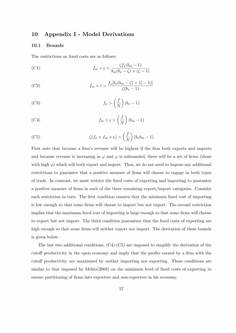
10 Appendix I - Model Derivations
10.1 Bounds
The restrictions on fixed costs are as follows:
(C1) fm + ε <ζfx(bm − 1)
bm(bx − ζ) + (ζ − 1)
(C2) fm + ε >fx[bx(bm − ζ) + (ζ − 1)]
ζ(bx − 1)
(C3) fx >
(f
N
)(bx − 1)
(C4) fm + ε >
(f
N
)(bm − 1)
(C5) ζ(fx + fm + ε) >
(f
N
)(bxbm − 1)
First note that because a firm’s revenue will be highest if the firm both exports and imports
and because revenue is increasing in ϕ and ϕ is unbounded, there will be a set of firms (those
with high ϕ) which will both export and import. Thus, we do not need to impose any additional
restrictions to guarantee that a positive measure of firms will choose to engage in both types
of trade. In contrast, we must restrict the fixed costs of exporting and importing to guarantee
a positive measure of firms in each of the three remaining export/import categories. Consider
each restriction in turn. The first condition ensures that the minimum fixed cost of importing
is low enough so that some firms will choose to import but not export. The second restriction
implies that the maximum fixed cost of importing is large enough so that some firms will choose
to export but not import. The third condition guarantees that the fixed costs of exporting are
high enough so that some firms will neither export nor import. The derivation of these bounds
is given below.
The last two additional conditions, (C4)-(C5) are imposed to simplify the derivation of the
cutoff productivity in the open economy and imply that the profits earned by a firm with the
cutoff productivity are maximized by neither importing nor exporting. These conditions are
similar to that imposed by Melitz(2003) on the minimum level of fixed costs of exporting to
ensure partitioning of firms into exporters and non-exporters in his economy.
57

We note that Figure 2 allows us to derive the bounds given above on the random component
of fixed costs of importing to ensure a positive measure of firms in each export/import category.
Let θ1 satisfy Φ0m(θ1) = Φ1
x(θ1) = Φxm(θ1) or
θ1 ≡ ζfx(bm − 1)bm(bx − ζ) + (ζ − 1)
. (62)
Let θ2 satisfy Φ1m(θ2) = Φ0
x(θ2) = Φxm(θ2) or
θ2 =fx[bx(bm − ζ) + (ζ − 1)]
ζ(bx − 1). (63)
Note that θ1 < θ2. Now condition (C1) above implies that θ < θ1 which we can see from the
figure implies a positive measure of firms choosing to import but not export. Condition (C2)
implies that θ > θ2 so that there is a positive measure of firms choosing to export but not
import.
We can derive similar conditions for partitioning firms in the economies with partial trade.
In the economy with no importing (bm = ζ = 1), equation (24) implies that firms with relative
productivity Φ ∈[
fN , fx
bx−1
)will not export while firms with Φ ≥ fx
bx−1 will export (which
is identical to the partitioning derived by Melitz(2003)). Similarly, in the economy with no
exporting (bx = ζ = 1), equation (25) implies that a firm with total fixed costs of importing
equal to θ will not import if their relative productivity satisfies Φ ∈[
fN , θ
bm−1
)and will import
otherwise.
10.2 Notation
For the full trading economy, using the cutoff functions in terms of Φ defined in equations
(24)-(26), we can define cutoffs functions in terms of ϕ as follows:
ϕji (ϕ
∗T , ε) ≡
(NΦj
i (ε)f
) 1σ−1
ϕ∗T i ∈ x, I, j ∈ 0, 1 (64)
ϕxm(ϕ∗T , ε) ≡(
NΦxm(ε)f
) 1σ−1
ϕ∗T (65)
Using equations (62) and (63), we can also define εj ≡ θj − fm for j = 1, 2.
For the economy with no importing, we denote the cutoff productivity for exporting as
ϕX(ϕ∗X) ≡(
Nfx
f(bx − 1)
) 1σ−1
ϕ∗X . (66)
58

Similarly, for the economy with no exporting, we denote the cutoff productivity for importing
for a firm with random importing cost equal to ε as
ϕI(ϕ∗I , ε) ≡(
N(fm + ε)f(bm − 1)
) 1σ−1
ϕ∗I . (67)
10.3 Firm Fractions
For each economy, the fraction of firms in each export/import status are given below.
νA(ϕ∗A, 0, 0) = 1 νA(ϕ∗A, 1, 0) = νA(ϕ∗A, 0, 1) = νA(ϕ∗A, 1, 1) = 0 (68)
νX(ϕ∗X , 0, 0) =(
11−G(ϕ∗X)
)[G(ϕX(ϕ∗X))−G(ϕ∗X)] (69)
νX(ϕ∗X , 1, 0) =(
11−G(ϕ∗X)
)[1−G(ϕX(ϕ∗X))] (70)
νX(ϕ∗X , 0, 1) = νX(ϕ∗X , 1, 1) = 0 (71)
νI(ϕ∗I , 0, 0) =
(1
1−G(ϕ∗I)
) [∫ ε
ε
(∫ ϕI(ϕ∗I ,ε)
ϕ∗I
g(z)dz
)h(ε)dε
](72)
νI(ϕ∗I , 0, 1) =
(1
1−G(ϕ∗I)
) [∫ ε
ε
(∫ ∞
ϕI(ϕ∗I ,ε)g(z)dz
)h(ε)dε
](73)
νI(ϕ∗I , 1, 0) = νI(ϕ∗I , 1, 1) = 0 (74)
νT (ϕ∗T , 0, 0) =(
11−G(ϕ∗T )
) [∫ ε1
ε
(∫ ϕ0m(ϕ∗T ,ε)
ϕ∗Tg(ϕ)dϕ
)h(ε)dε+
∫ ε2
ε1
(∫ ϕxm(ϕ∗T ,ε)
ϕ∗Tg(ϕ)dϕ
)h(ε)dε
∫ ε
ε2
(∫ ϕ0x(ϕ∗T ,ε)
ϕ∗Tg(ϕ)dϕ
)h(ε)dε
](75)
νT (ϕ∗T , 0, 1) =(
11−G(ϕ∗T )
) [∫ ε1
ε
(∫ ϕ1x(ϕ∗T ,ε)
ϕ0m(ϕ∗T ,ε)
g(ϕ)dϕ
)h(ε)dε
](76)
νT (ϕ∗T , 1, 0) =(
11−G(ϕ∗T )
) [∫ ε
ε2
(∫ ϕ1m(ϕ∗T ,ε)
ϕ0x(ϕ∗T ,ε)
g(ϕ)dϕ
)h(ε)dε
]
(77)
59
νT (ϕ∗T , 1, 1) =(
11−G(ϕ∗T )
) [∫ ε1
ε
(∫ ∞
ϕ1x(ϕ∗T ,ε)
g(ϕ)dϕ
)h(ε)dε +
∫ ε2
ε1
(∫ ∞
ϕxm(ϕ∗T ,ε)g(ϕ)dϕ
)h(ε)dε
+∫ ε
ε2
(∫ ∞
ϕ1m(ϕ∗T ,ε)
g(ϕ)dϕ
)h(ε)dε
](78)
10.4 Aggregate Price Indexes and Average Productivities
In the autarkic equilibrium, (S = A) equations (2), (6), and (7) imply that the aggregate price
index is given by
PA =[
1ρA
] [(MA(ϕ∗A)
1−G(ϕ∗A)
) ∫ ∞
ϕ∗Aϕσ−1g(ϕ)dϕ
] 11−σ
(79)
or
PA = MA(ϕ∗A)1
1−σ p
[1
MA(ϕ∗A)(1−G(ϕ∗A))
(∫ ∞
ϕ∗Aϕσ−1g(ϕ)dϕ
)] 1σ−1
(80)
Thus, our measures of average productivity in autarky are given by
bA(ϕ∗A, 0, 0) =
[1
(1−G(ϕ∗A))
(∫ ∞
ϕ∗Aϕσ−1g(ϕ)dϕ
)] 1σ−1
(81)
bA(ϕ∗A, 1, 0) = bA(ϕ∗A, 0, 1) = bA(ϕ∗A, 1, 1) = 0, (82)
where we have adopted the convention that average productivity for an export/import category
with a zero measure of firms equals zero.
In the economy with no importing, (S = X) equations (2), (6), (7), and (8) imply that the
aggregate price index is given by
PX =[
1ρA
] [(MX(ϕ∗X)
1−G(ϕ∗X)
) (∫ ϕX(ϕ∗X)
ϕ∗Xϕσ−1g(ϕ)dϕ +
∫ ∞
ϕX(ϕ∗X)(1 + Nτσ−1)ϕσ−1g(ϕ)dϕ
)] 11−σ
,
(83)
or
PX =[
1ρA
] [(MX(ϕ∗X , 0, 0)
νX(ϕ∗X , 0, 0)(1−G(ϕ∗X))
) (∫ ϕX(ϕ∗X)
ϕ∗Xϕσ−1g(ϕ)dϕ
)
+(
MX(ϕ∗X , 1, 0)bx
νX(ϕ∗X , 1, 0)(1−G(ϕ∗X))
) (∫ ∞
ϕX(ϕ∗X)ϕσ−1g(ϕ)dϕ
)] 11−σ
. (84)
60

Thus, our measures of average productivity in the partial trading economy with exporting
bX(ϕ∗X , 0, 0) =
[(1
νX(ϕ∗X , 0, 0)(1−G(ϕ∗X))
) ∫ ϕX(ϕ∗X)
ϕ∗Xϕσ−1g(ϕ)dϕ
] 1σ−1
(85)
bX(ϕ∗X , 1, 0) =
[(bx
νX(ϕ∗X , 1, 0)(1−G(ϕ∗X))
) ∫ ∞
ϕX(ϕ∗X)ϕσ−1g(ϕ)dϕ
] 1σ−1
(86)
bX(ϕ∗X , 0, 1) = bX(ϕ∗X , 1, 1) = 0. (87)
In the economy with no exporting, (S = I) equations (2), (6), and (7) imply that the
aggregate price index is given by
PI =[
1ρA
] [(MI(ϕ∗I , 0, 0)1−G(ϕ∗I )
) (∫ ε
ε
(∫ ϕI(ϕ∗I ,ε)
ϕ∗Iϕσ−1g(ϕ)dϕ
)h(ε)dε
+∫ ε
ε
(∫ ∞
ϕI(ϕ∗I ,ε)λσ−1ϕσ−1g(ϕ)dϕ
)h(ε)dε
)] 1σ−1
(88)
Thus, our measures of average productivity in the partial trading economy with importing are
bI(ϕ∗I , 0, 0) =
[(1
νI(ϕ∗I , 0, 0)(1−G(ϕ∗I ))
) ∫ ε
ε
(∫ ϕI(ϕ∗I ,ε)
ϕ∗Iϕσ−1g(ϕ)dϕ
)h(ε)dε
] 1σ−1
(89)
bI(ϕ∗I , 0, 1) =
[(bm
νI(ϕ∗I , 0, 1)(1−G(ϕ∗I ))
) ∫ ε
ε
(∫ ∞
ϕI(ϕ∗I ,ε)ϕσ−1g(ϕ)dϕ
)h(ε)dε
] 1σ−1
(90)
bI(ϕ∗I , 1, 0) = bI(ϕ∗I , 1, 1) = 0. (91)
Using the same approach as in the previous three economies and using Figure 2, we have the
following average productivities across groups of firms in the full trading equilibrium
bT (ϕ∗T , 0, 0) =
[(1
νT (ϕ∗T , 0, 0)(1−G(ϕ∗T ))
) (∫ ε1
ε
(∫ ϕ0m(ϕ∗T ,ε)
ϕ∗Tϕσ−1g(ϕ)dϕ
)h(ε)dε
+∫ ε2
ε1
(∫ ϕxm(ϕ∗T ,ε)
ϕ∗Tϕσ−1g(ϕ)dϕ
)h(ε)dε
∫ ε
ε2
(∫ ϕ0x(ϕ∗T ,ε)
ϕ∗Tϕσ−1g(ϕ)dϕ
)h(ε)dε
)] 1σ−1
(92)
bT (ϕ∗T , 0, 1) =
[(bm
νT (ϕ∗T , 0, 1)(1−G(ϕ∗T ))
) (∫ ε1
ε
(∫ ϕ1x(ϕ∗T ,ε)
ϕ0m(ϕ∗T ,ε)
ϕσ−1g(ϕ)dϕ
)h(ε)dε
)] 1σ−1
(93)
61

bT (ϕ∗T , 1, 0) =
[(bx
νT (ϕ∗T , 1, 0)(1−G(ϕ∗T ))
) (∫ ε
ε2
(∫ ϕ1m(ϕ∗T ,ε)
ϕ0x(ϕ∗T ,ε)
ϕσ−1g(ϕ)dϕ
)h(ε)dε
)] 1σ−1
(94)
bT (ϕ∗T , 1, 1) =
[(bxbm
νT (ϕ∗T , 1, 1)(1−G(ϕ∗T ))
) (∫ ε1
ε
(∫ ∞
ϕ1x(ϕ∗T ,ε)
ϕσ−1g(ϕ)dϕ
)h(ε)dε
+∫ ε2
ε1
(∫ ∞
ϕxm(ϕ∗T ,ε)ϕσ−1g(ϕ)dϕ
)h(ε)dε +
∫ ε
ε2
(∫ ∞
ϕ1m(ϕ∗T ,ε)
ϕσ−1g(ϕ)dϕ
)h(ε)dε
)] 1σ−1
(95)
10.5 Average Profits
Using equation (14), average profits across firms in autarky equals
πA(ϕ∗A, 0, 0) =(
1νA(ϕ∗A, 0, 0)
) (1
1−G(ϕ∗A)
) ∫ ∞
ϕ∗A
(rA(ϕ, 0, 0)
σ− f
)g(ϕ)dϕ (96)
or, using equations (18) and (68)
πA(ϕ∗A, 0, 0) = ϕ∗A1−σf
∫ ∞
ϕ∗A
(ϕσ−1
1−G∗A
)g(ϕ)dϕ− f (97)
or, using (18) and (81),
πA(ϕ∗A, 0, 0) =rA(bA(ϕ∗A, 0, 0), 0, 0)
σ− f (98)
Finally, since the other export/import categories have measure zero firms in autarky, we set
πA(ϕ∗A, 1, 0) = πA(ϕ∗A, 0, 1) = πA(ϕ∗A, 1, 1) = 0.
In the economy with no importing, using (14), we have
πX(ϕ∗X , 0, 0) =(
1νX(ϕ∗X , 0, 0)
) (1
1−G(ϕ∗X)
) ∫ ϕX(ϕ∗X)
ϕ∗X
(rX(ϕ, 0, 0)
σ− f
)g(ϕ)dϕ (99)
or using (20) and (69)
πX(ϕ∗X , 0, 0) =(
1νX(ϕ∗X , 0, 0)
)ϕ∗X
1−σf
∫ ϕX(ϕ∗X)
ϕ∗X
(ϕσ−1
1−G∗X
)g(ϕ)dϕ− f (100)
or using (20) and (85),
πX(ϕ∗X , 0, 0) =
(rX(bX(ϕ∗X , 0, 0), 0, 0)
σ
)− f. (101)
In a similar manner, we can derive
πX(ϕ∗X , 1, 0) =
(rX(bX(ϕ∗X , 1, 0), 0, 0)
σ
)− (f + Nfx). (102)
62
Finally, πX(ϕ∗X , 0, 1) = πX(ϕ∗X , 1, 1) = 0.
In the economy with no exporting, using similar methods to those for autarky or the no
importing economy, we can derive
πI(ϕ∗I , 0, 0) =
(rI(bI(ϕ∗I , 0, 0), 0, 0)
σ
)− f. (103)
Using equation (14), we write
πI(ϕ∗I , 0, 1) =(
1νI(ϕ∗I , 0, 1)(1−G(ϕ∗I ))
) ∫ ε
ε
(∫ ∞
ϕI(ϕ∗I ,ε)
(rI(ϕ, 0, 1)
σ− (f + N(fm + ε))
)g(ϕ)dϕ
)h(ε)dε
(104)
or using (21), (73) and (90),
πI(ϕ∗I , 0, 1) =
(rI(bI(ϕ∗I , 0, 1), 0, 0)
σ
)− (f + Nfm) (105)
−(
N
νI(ϕ∗I , 0, 1)(1−G(ϕ∗I ))
) ∫ ε
ε
(∫ ∞
ϕI(ϕ∗I ,ε)ε g(ϕ)dϕ
)h(ε)dε, (106)
or
πI(ϕ∗I , 0, 1) =
(rI(bI(ϕ∗I , 0, 1), 0, 0)
σ
)− (f + N(fm + εI(0, 1))), (107)
where εI(0, 1) is the average random component of fixed import costs across firms which import
in this economy. Finally, πI(ϕ∗I , 1, 0) = πI(ϕ∗I , 1, 1) = 0.
Using similar methods, we can derive average profits for each group of firms in the full trading
economy:
πT (ϕ∗T , 0, 0) =
(rT (bT (ϕ∗T , 0, 0), 0, 0)
σ
)− f (108)
πT (ϕ∗T , 1, 0) =
(rT (bT (ϕ∗T , 1, 0), 0, 0)
σ
)− (f + Nfx) (109)
πT (ϕ∗T , 0, 1) =
(rT (bT (ϕ∗T , 0, 1), 0, 0)
σ
)− (f + Nfm)
−(
N
νT (ϕ∗T , 0, 1)
) ∫ ε1
ε
(∫ ϕ1x(ϕT ,ε)
ϕ0m(ϕ∗T ,ε)
ε g(ϕ)dϕ
)h(ε)dε, (110)
or
πT (ϕ∗T , 0, 1) =
(rT (bT (ϕ∗T , 0, 1), 0, 0)
σ
)− (f + N(fm + εT (0, 1))), (111)
63

where εT (0, 1) is the average random component of fixed import costs across firms who import
but do not export.
πT (ϕ∗T , 1, 1) =
(rT (bT (ϕ∗T , 1, 1), 0, 0)
σ
)− (f + ζN(fx + fm))
−(
ζN
νT (ϕ∗T , 1, 1)
) [∫ ε1
ε
(∫ ∞
ϕ1x(ϕ∗T ,ε)
ε g(ϕ)dϕ
)h(ε)dε.
+∫ ε2
ε1
(∫ ∞
ϕxm(ϕ∗T ,ε)ε g(ϕ)dϕ
)h(ε)dε
+∫ ε
ε2
(∫ ∞
ϕ1m(ϕ∗T ,ε)
ε g(ϕ)dϕ
)h(ε)dε
], (112)
or
πT (ϕ∗T , 1, 1) =
(rT (bT (ϕ∗T , 1, 1), 0, 0)
σ
)− (f + ζN(fx + fm + εT (1, 1))), (113)
where εT (1, 1) is the average random part of fixed import costs across firms which both import
and export.
10.6 Equilibrium Mass of Firms
For notational convenience, we drop the equilibrium cutoff productivity arguments in the func-
tions below. In each of the four economies average revenue across all firms is given by
rS =∑
d∈0,12νS(d)rS(bS(d), 0, 0). (114)
and aggregate revenue is given by RS = rSMS = L, where the last inequality follows from the
property that GNP equals payments to labor. Thus, in each economy the equilibrium mass of
operating firms must be given by
MS =L
rS
. (115)
Average profits in each economy can be written as
πS = νS(0, 0)
(rS(bS(0, 0), 0, 0))
σ− f
)+ νS(1, 0)
(rS(bS(1, 0), 0, 0))
σ− (f + Nfx)
)
+νS(0, 1)
(rS(bS(0, 1), 0, 0))
σ− (f + N(fm + εS(0, 1)))
)
+νS(1, 1)
(rS(bS(1, 1), 0, 0))
σ− (f + ζN(fx + fm + εS(1, 1)))
), (116)
64

where εI(0, 1), εT (0, 1), and εT (1, 1) are defined in the previous section and all other εS(d) (those
for categories with measure zero of firms) are set to zero. This implies that
πS =rS
σ− f − νS(1, 0)Nfx − νS(0, 1)N(fm + εS(0, 1))− νS(1, 1)ζN(fx + fm + εS(1, 1)). (117)
Hence, using equation (115), we have the equilibrium mass of firms in economy S:
MS =L
σ[πS + f + νS(1, 0)Nfx + νS(0, 1)N(fm + εS(0, 1)) + νS(1, 1)ζN(fx + fm + εS(1, 1))].
(118)
65

11 Appendix II: Proofs of Propositions
Proof of Proposition 1:
The cutoff productivity for operation in the autarkic equilibrium, ϕ∗A, must satisfy the closed
economy version of equation (17):
∫ ε
επA(ϕ∗A, 0, 0, ε)h(ε)dε = 0. (119)
or using equations (4) and (14), we have
rA(ϕ∗A, 0, 0) = σf, (120)
where rA(·) is given by equation 12 evaluated at d = (0, 0). For the full trading economy
we must show that (0, 0) = argmaxd∈0,12 π(ϕ∗T , d, ε) ∀ ε when r(ϕ∗T , 0, 0) = σf . It can
easily be shown that when r(ϕ∗T , 0, 0) = σf , then ∀ ε ∈ (ε, ε) condition (C3) implies that
π(ϕ∗T , 0, 0, ε) > π(ϕ∗T , 1, 0, ε), condition (C4) implies that π(ϕ∗T , 0, 0, ε) > π(ϕ∗S, 0, 1, ε), and (C5)
implies π(ϕ∗T , 0, 0, ε) > π(ϕ∗T , 1, 1, ε). Thus, the cutoff condition given by equation (17) becomes∫ εε π(ϕ∗T , 0, 0, ε)h(ε)d(ε) = 0 which is clearly satisfied at our candidate ϕ∗T . For the economy
with no trade in intermediates we must show that (0) = argmaxdx∈0,1 π(ϕ∗X , dx, 0, ε) ∀ ε when
r(ϕ∗X , 0, 0) = σf . It can easily be shown that when r(ϕ∗X , 0, 0) = σf , then ∀ ε ∈ (ε, ε) condition
(C3) implies that π(ϕ∗X , 0, 0, ε) > π(ϕ∗X , 1, 0, ε). Thus, the cutoff condition given by equation
(17) becomes∫ εε π(ϕ∗X , 0, 0, ε)h(ε)d(ε) = 0 which is clearly satisfied at our candidate ϕ∗X .
For the economy with no trade in final goods we must show that (0) = argmaxdm∈0,1 π(ϕ∗X , 0, dm, ε)
∀ ε when r(ϕ∗X , 0, 0) = σf . It can easily be shown that when r(ϕ∗I , 0, 0) = σf , then ∀ ε ∈ (ε, ε)
condition (C4) implies that π(ϕ∗I , 0, 0, ε) > π(ϕ∗I , 0, 1, ε). Thus, the cutoff condition given by
equation (17) becomes∫ εε π(ϕ∗I , 0, 0, ε)h(ε)d(ε) = 0 which is clearly satisfied at our candidate ϕ∗I .
Proof of Proposition 2:
(i.) ϕ∗A exists and is unique.
Define the following function of ϕ:
γA(ϕ) ≡ ϕ1−σf
∫ ∞
ϕzσ−1g(z)dz − f [1−G(ϕ)]. (121)
66

Note that γA(·) > 0 ∀ ϕ because
γA(ϕ) = f
[∫ ∞
ϕ
(z
ϕ
)σ−1
g(z)dz − (1−G(ϕ))
], (122)
which is clearly positive for σ > 1. The equilibrium cutoff level in autarky, ϕ∗A satisfies
γA(ϕ∗A) = ξfe. (123)
Following Melitz, we will show that γA(ϕ) is monotonically decreasing from ∞ to 0 on (0,∞).
The derivative of this function is given by
γ′A(ϕ) = (1− σ)[γA(ϕ) + f [1−G(ϕ)]
ϕ
]< 0, (124)
where the inequality follows from σ > 1. The elasticity is
γ′A(ϕ)ϕγA(ϕ)
= (1− σ)[1 +
f [1−G(ϕ)]γA(ϕ)
]< (1− σ) < 0. (125)
Since the elasticity is negative and bounded away from zero, γA(ϕ) is decreasing to 0 as ϕ goes
to ∞. Also, we see by inspection that limϕ→0 γA(ϕ) = ∞. This implies that the solution to
equation (123) exists and is unique.
Turning to the economies with trade, we define the following functions for i ∈ 1, 2, 3 and
j ∈ 0, 1, 2, 3, 4, X, I:
δi(ϕ, ϕj(ϕ, ε), εL, εH) ≡ ϕ1−σBi
∫ εH
εL
(∫ ∞
ϕj(ϕ,ε)zσ−1g(z)dz
)h(ε)dε
−∫ εH
εL
(Ci(ε)
∫ ∞
ϕj(ϕ,ε)g(z)dz
)h(ε)dε, (126)
where
B1 = f(bx − 1) B2 = f(bm− 1) B3 = f(bx − 1)(bm − 1), (127)
C1(ε) = Nfx C2(ε) = N(fm + ε) C3(ε) = N(ζ − 1)(fx + fm + ε), (128)
ϕo(ϕ, ε) ≡ ϕ1x(ϕ, ε) ϕ1(ϕ, ε) ≡ ϕo
m(ϕ, ε) ϕ2(ϕ, ε) ≡ ϕxm(ϕ, ε)
ϕ3(ϕ, ε) ≡ ϕ1m(ϕ, ε) ϕ4(ϕ, ε) ≡ ϕo
x(ϕ, ε), (129)
and ϕX(ϕ, ε) and ϕI(ϕ, ε) are given by equations (66) and (67) respectively.
(ii.) ϕ∗X exists and is unique.
67

Define the following function of ϕ:
γX(ϕ) = γA(ϕ) + δ1(ϕ, ϕX(ϕ), ε, ε). (130)
Note that γX > 0 ∀ ϕ because γA(ϕ) > 0 and
δ1(ϕ, ϕX , ε, ε) = Nfx
[∫ ∞
ϕ
(z
ϕ
)σ−1
− (1−G(ϕ))
], (131)
which is clearly positive for σ > 1. The equilibrium cutoff level in economy X, ϕ∗X , satisfies
γX(ϕ∗X) = ξfe. (132)
We will argue that γX(·)is monotonically decreasing from ∞ to 0 on (0,∞), proving existence
and uniqueness of the cutoff productivity in the economy with no importing. Above, we argued
that the first function on the right-hand side of (163) has this property. The elasticity of the
second function on the right-hand side with respect to ϕ is given by
∂ ln δ1
∂ ln ϕ= (1− σ)
[1 +
νX(ϕ, 1, 0)(1−G(ϕ∗X))Nfx
δ1
]< (1− σ) < 0. (133)
Since the elasticity is negative and bounded away from zero, δ1 is decreasing to 0 as ϕ goes to
∞. Also, we see by inspection that limϕ→0 δ1 = ∞. Thus, γX(·) is the sum of two functions
which are decreasing from ∞ to 0 on (0,∞) and so ϕ∗X exists and is unique.
(iii.) ϕ∗I exists and is unique.
Define the following function of ϕ:
γI(ϕ) = γA(ϕ) + δ2(ϕ, ϕI(ϕ), ε, ε). (134)
Note that γM (ϕ) > 0 ∀ ϕ because γA(ϕ) > 0 and
δ2(ϕ, ϕI , ε, ε) =∫ ε
εN(fm + ε)
(∫ ∞
ϕI(ϕ,ε)
[(z
ϕI(ϕ, ε)
)σ−1
− 1
]g(z)dz
)h(ε)dε (135)
which is clearly positive when σ > 1. The equilibrium cutoff level in economy M , ϕ∗I , satisfies
γI(ϕ∗I ) = ξfe. (136)
We will argue that γI(·)is monotonically decreasing from ∞ to 0 on (0,∞), proving existence
and uniqueness of the cutoff productivity in the economy with no exporting. Above, we argued
68

that the first function on the right-hand side of (164) has this property. The elasticity of the
second function on the right-hand side with respect to ϕ is given by
∂ ln δ2
∂ ln ϕ= (1− σ)
[1 +
νI(ϕ, 0, 1)(1−G(ϕ∗I ))N(fm + εI(0, 1)δ2
]< (1− σ) < 0. (137)
Since the elasticity is negative and bounded away from zero, δ2 is decreasing to 0 as ϕ goes to
∞. Also, we see by inspection that limϕ→0 δ2 = ∞. Thus, γI(·) is the sum of two functions
which are decreasing from ∞ to 0 on (0,∞) and so ϕ∗I exists and is unique.
(iv.) ϕ∗T exists and is unique.
Define the following function of ϕ:
γ1(ϕ) ≡∑
i∈1,3δi(ϕ, ϕ0(ϕ, ε), ε, ε1) (138)
γ2(ϕ) ≡ δ2(ϕ, ϕ1(ϕ, ε), ε, ε1) (139)
γ3(ϕ) ≡∑
i∈1,2,3δi(ϕ, ϕ2(ϕ, ε), ε1, ε2) (140)
γ4(ϕ) ≡∑
i∈2,3δi(ϕ, ϕ3(ϕ, ε), ε2, ε) (141)
γ5(ϕ) ≡ δ1(ϕ, ϕ4(ϕ, ε), ε2, ε) (142)
Using arguments similar to those used in parts (ii.) and (iii.) above, we can show that each of
the γi(ϕ) functions are positive-valued. We define the following function of ϕ
γT (ϕ) ≡ γA(ϕ) +5∑
i=1
γi(ϕ) (143)
and note that it is positive-valued. Through manipulation of equation (35), we can show that
the equilibrium cutoff productivity level in trade, ϕ∗T satisfies
γT (ϕ∗T ) = ξfe. (144)
We will argue that this function is monotonically decreasing from ∞ to 0 on (0,∞) implying
that ϕ∗T exists and is unique. We will do so by showing that each function in the sum on the
right-hand side of (143) has this property.
We already showed in part (i.) of this proof that γA(·) has this property. Let γj denote the
elasticity of γj with respect to ϕ for j = 1, ..., 5. Dropping the arguments of functions, we can
69
derive
γ1 = (1− σ)
1 +
∑i∈1,3
∫ ε1ε
(Ci
∫∞ϕ0
g(z)dz)
h(ε)dε
γ1
< (1− σ) < 0. (145)
Hence, since the elasticity of this function is negative and bounded away from 0, it must be
monotonically decreasing on (0,∞). By inspection, we also see that the limit of this function as
ϕ → 0 equals ∞ because limϕ→0ϕ0(ϕ, ε) = 0 for any ε.
Similarly, we have
γ2 = (1− σ)
1 +
∫ ε1ε
(C2
∫∞ϕ1
g(z)dz)
h(ε)dε
γ2
< (1− σ) < 0, (146)
γ3 = (1− σ)
1 +
∑3i=1
∫ ε2ε1
(Ci
∫∞ϕ2
g(z)dz)
h(ε)dε
γ3
< (1− σ) < 0, (147)
γ4 = (1− σ)
1 +
∑3i=2
∫ εε2
(Ci
∫∞ϕ3
g(z)dz)
h(ε)dε
γ4
< (1− σ) < 0, (148)
and
γ5 = (1− σ)
1 +
∫ εε2
(C1
∫∞ϕ4
g(z)dz)
h(ε)dε
γ5
< (1− σ) < 0. (149)
Furthermore, the limit of each of these functions as ϕ → 0 equals ∞. Thus, each of these
functions are monotonically decreasing from ∞ to 0 on (0,∞). These results imply that γT (ϕ)
is the sum of functions which decrease monotonically from ∞ to 0 on (0,∞) and, so, must also
have this property. Thus, the ϕ∗T which satisfies equation (144) exists and is unique.
Proof of Proposition 3:
The equilibrium equations given by (123), (132), (136), and (144) for the respective economies
imply
ξfe = γA(ϕ∗A)
= γA(ϕ∗X) + δ1(ϕ∗X , ϕX(ϕ∗X), ε, ε)
= γA(ϕ∗I ) + δ2(ϕ∗I , ϕI(ϕ∗I ), ε, ε).
= γA(ϕ∗T ) +5∑
i=1
γi(ϕ∗T ).
Now since δ1(·), δ2(·), and γi(·) for i ∈ 1, 5 are positive-valued and since γA(ϕ) is a decreasing
function, we have ϕ∗A < ϕ∗X , ϕ∗A < ϕ∗I , and ϕ∗A < ϕ∗T .
70

Note that ϕ∗X = ϕ∗T when bm = ζ = 1 and ϕ∗I = ϕ∗T when bx = ζ = 1. We will demonstrate
that ϕ∗T is increasing in bm, increasing in bx, and decreasing in ζ. Now a movement from the
economy with no importing to the economy with full trade can be represented by an increase in
bm and, possibly, a decrease in ζ. Thus, if we show that the cutoff productivity in the full trading
equilibrium is increasing in bm and decreasing in ζ, then we have the result that ϕ∗X < ϕ∗T . Using
a similar argument for increases in bx, we have the result that ϕ∗I < ϕ∗T .
Let the elasticity of a function f(z) with respect to z be written as fz. Then equation (144)
implies
ϕ∗zT = −(
γzT
γϕT
)(150)
From equation (143), we can derive the following elasticities:
γϕT =
[(1− σ)ϕ1−σf
γT
] [∫ ∞
ϕzσ−1g(z)dz
+∫ ε1
ε
(bm(bx − 1)
∫ ∞
ϕ0
zσ−1g(z)dz + (bm − 1)∫ ∞
ϕ1
zσ−1g(z)dz
)h(ε)dε
+∫ ε2
ε1
((bmbx − 1)
∫ ∞
ϕ2
zσ−1g(z)dz
)h(ε)dε
+∫ ε
ε2
(bx(bm − 1)
∫ ∞
ϕ3
zσ−1g(z)dz + (bx − 1)∫ ∞
ϕ4
zσ−1g(z)dz
)h(ε)dε
]
< 0 (151)
γbmT =
[bIϕ
1−σf
γT
] [∫ ε1
ε
((bx − 1)
∫ ∞
ϕ0
zσ−1g(z)dz +∫ ∞
ϕ1
zσ−1g(z)dz
)h(ε)dε
+∫ ε2
ε1
(bx
∫ ∞
ϕ2
zσ−1g(z)dz
)h(ε)dε
+∫ ε
ε2
(bx
∫ ∞
ϕ3
zσ−1g(z)dz
)h(ε)dε
]
> 0 (152)
γbxT =
[bxϕ1−σf
γT
] [∫ ε1
ε
(bm
∫ ∞
ϕ0
zσ−1g(z)dz
)h(ε)dε
+∫ ε2
ε1
(bm
∫ ∞
ϕ2
zσ−1g(z)dz
)h(ε)dε
+∫ ε
ε2
((bm − 1)
∫ ∞
ϕ3
zσ−1g(z)dz +∫ ∞
ϕ4
zσ−1g(z)dz
)h(ε)dε
]
71

> 0 (153)
γζT =
[−ζN
γT
] [∫ ε1
ε
(∫ ∞
ϕ0
(fx + fm + ε)g(z)dz
)h(ε)dε
+∫ ε2
ε1
(∫ ∞
ϕ2
(fx + fm + ε)g(z)dz
)h(ε)dε
+∫ ε
ε2
(∫ ∞
ϕ3
(fx + fm + ε)g(z)dz
)h(ε)dε
]
< 0 (154)
Hence, using equation (150) and the signs of these elasticities, we have
ϕ∗bmT > 0 ϕ∗bx
T > 0 ϕ∗ζT < 0 (155)
This proves the remaining parts of the proposition.
Proof of Proposition 4:
Inspection of equations (??), (??), (??), and (??) and the result that πA < πX < πT and πA < πI
shows that MA > MX , MA > MI , and MA > MT .
Equation (115) implies that if we can show that rX < rT and rI < rT , then we have the
remaining results. To demonstrate these average revenue rankings, it is enough to show that rT
is increasing in bm, increasing in bx, and decreasing in ζ.
Changing the variable of integration in the average revenue calculations from ϕ to Φ allows
us to write average profits in the full trading equilibrium as
rT =
(σN
σσ−1 f
11−σ ϕ∗T
(σ − 1)(1−G(f/N)
)[∫ ε1
ε
(∫ Φ1
f/NΦ
1σ−1 g(Φ)dΦ+bI
∫ Φ0
Φ1
Φ1
σ−1 g(Φ)dΦ+bxbI
∫ ∞
Φ0
Φ1
σ−1 g(Φ)dΦ
)h(ε)dε
+∫ ε2
ε1
(∫ Φ2
f/NΦ
1σ−1 g(Φ)dΦ + bxbI
∫ ∞
Φ2
Φ1
σ−1 g(Φ)dΦ
)h(ε)dε
∫ ε
ε2
(∫ Φ4
f/NΦ
1σ−1 g(Φ)dΦ + bx
∫ Φ3
Φ4
Φ1
σ−1 g(Φ)dΦ + bxbI
∫ ∞
Φ3
Φ1
σ−1 g(Φ)dΦ
)h(ε)dε
]
Now since, ϕ∗bmT > 0, bx > 1, bm > 1, and ∂Φj
∂bm≤ 0 ∀j, then the derivative of the above expression
for average revenue with respect to bm is positive. Similarly, because ∂Φj
∂bx≤ 0 ∀j, the derivative
with respect to bx is positive. Finally, since ∂Φj
∂ζ ≥ 0 ∀j, the derivative of average revenue in
the trading equilibrium with respect ζ is decreasing. These results imply that average revenue
72
is higher in the full trading equilibrium than in either of the partial trading equilibrium and
proves the proposition.
Proof of Proposition 5:
Welfare in this economy is the inverse of the price index. Hence, in autarky, equation (??)
aggregate welfare is given by
WA =1
PA
= M1
σ−1A AρbA(ϕ∗A) (156)
Furthermore, equations (??) and (13) and recalling that RA = wL = L allows us to derive
bA(ϕ∗A) =[
L
MAσf
) 1σ−1
ϕ∗A (157)
Substituting this into equation (156) gives
WA = Aρ
[L
σf
] 1σ−1
ϕ∗A (158)
Similarly, from equation (31) in the trading equilibrium, we have
WT =1
PT
= MC
1σ−1 AρbT (ϕ∗T ) (159)
Furthermore, equations (32) and (13) and recalling that RT = wL = L allows us to derive
bT (ϕ∗T ) =[
L
MCσf
] 1σ−1
ϕ∗T (160)
Substituting this into equation (159) gives
WT = Aρ
[L
σf
] 1σ−1
ϕ∗T (161)
Now since ϕ∗A < ϕ∗T , we have WA < WT .
Proof of Proposition 6:
Recall the following revenue functions in autarky and trade
rA(ϕ) = (σfϕσ−1)ϕ∗A1−σ rT (ϕ, d) = (bdx
x bdmm )(σfϕσ−1)ϕ∗T
1−σ (162)
(i.) rT (ϕ, 0, 0) < rA(ϕ) follows directly from Proposition 1.
Consider two economies with partial trade. First, the open economy considered here with
ζ = bm = 1. This would be an economy with only exports and no imports and we label all
73
variables associated with this economy with an X. This is the analog to the open economy that
Melitz studied. Second, consider the open economy considered here with ζ = bx = 1. This is
an economy with only imports and no exports and we label all variables associated with this
economy with an M . Define the following functions
γX(ϕ) ≡ γA(ϕ) + δ1(ϕ, ϕX , ε, ε) (163)
where ϕX equals ϕ0 evaluated at ζ = bm = 1, and
γM (ϕ) ≡ γA(ϕ) + δ2(ϕ, ϕM , ε, ε) (164)
where ϕM equals ϕ1 evaluated at ζ = bx = 1. Now, the equilibrium cutoff productivity for
operation in each economy satisfies
γX(ϕ∗X) = ξfe (165)
γM (ϕ∗M ) = ξfe (166)
Let the associated revenue functions in each economy be denoted rX(ϕ, d) and rM (ϕ, d). We
now derive the following result
rA(ϕ) < rX(ϕ, 1, 0) < rT (ϕ, 1, 1) (167)
We first note that limbx→1rX(ϕ, 1, 0) = rA(ϕ). Now if we can show that rX(ϕ, 1, 0) is increasing
in bx, then we have proved the first inequality. Recall that rX(ϕ, 1, 0) = bx
[ϕ
ϕ∗X
]σ−1σf . The
elasticity of this function with respect to bx is given by(
∂rX(ϕ, 1, 0)∂bx
) (bx
rX(ϕ, 1, 0)
)= 1 + (1− σ)
(∂ϕ∗X∂bx
) (bx
ϕ∗X
)(168)
Differentiating (165) with respect to bx and rearranging gives
(∂ϕ∗X∂bx
) (bx
ϕ∗X
)= −
(∂γX∂bx
) (bxγX
)(
∂γX∂ϕ
) (ϕ∗XγX
) (169)
Now if we derive these elasticities and substitute into equation (168), we derive the following
Sign
(∂rX(ϕ, 1, 0)
∂bx
) (bx
rX(ϕ, 1, 0)
)= Sign
∫ ∞
ϕ∗Xzσ−1g(z)dz −
∫ ∞
ϕX
zσ−1g(z)dz
. (170)
Now, since ϕ∗X < ϕX , this expression must be positive, so rX(ϕ, 1, 0) is increasing in bx and
rA(ϕ) < rX(ϕ, 1, 0) for all ϕ.
74
Next, note that limbm→1rT (ϕ, 1, 1) = rX(ϕ, 1, 0). Now if we can show that rT (ϕ, 1, 1) is increas-
ing in bm, then we have proved the second inequality. Recall that rT (ϕ, 1, 1) = bxbI
[ϕ
ϕ∗T
]σ−1σf .
The elasticity of this function with respect to bm is given by
(∂rT (ϕ, 1, 1)
∂bm
) (bm
rT (ϕ, 1, 1)
)= 1 + (1− σ)
(∂ϕ∗T∂bm
) (bm
ϕ∗T
)(171)
Differentiating (144) with respect to bm and rearranging gives
(∂ϕ∗T∂bm
) (bm
ϕ∗T
)= −
(∂γT∂bm
) (bmγT
)(
∂γT∂ϕ
) (ϕ∗TγT
) (172)
Now if we derive these elasticities and substitute into equation (173), we derive the following
Sign
(∂rT (ϕ, 1, 1)
∂bm
) (bm
rT (ϕ, 1, 1)
)= Sign
∫ ε2
ε1
[∫ ∞
ϕ∗Tzσ−1g(z)dz −
∫ ∞
ϕ1
zσ−1g(z)dz
]h(ε)dε
+∫ ε3
ε2
[∫ ∞
ϕ∗Tzσ−1g(z)dz −
∫ ∞
ϕ2
zσ−1g(z)dz
]h(ε)dε
+∫ ε4
ε3
[∫ ∞
ϕ∗Tzσ−1g(z)dz −
∫ ∞
ϕ4
zσ−1g(z)dz
]h(ε)dε
+bx
∫ ε4
ε3
[∫ ∞
ϕ4
zσ−1g(z)dz −∫ ∞
ϕ3
zσ−1g(z)dz
]h(ε)dε
(173)
Now, we know that ϕ∗T < ϕj for j ∈ 1, 2, 4 and ε > ε. We also have ϕ4 < ϕ3 for ε ∈ε2, ε. These inequalities imply that the elasticity in equation (173) is positive. Thus, we
have demonstrated that rT (ϕ, 1, 1) is increasing in bm and so rX(ϕ, 1, 0) < rT (ϕ, 1, 1). Finally,
combining these two results, we have rA(ϕ) < rT (ϕ, 1, 1) for all ϕ.
Using similar methods, we can argue that limbm→1 rM (ϕ, 0, 1) → rA(ϕ) and that rM (ϕ, 0, 1) is
increasing in bm. Together, these imply that rA(ϕ) < rM (ϕ, 0, 1). (Derivations omitted for now.)
Proof of Proposition 6 (Incomplete)
Proof of Proposition 7 (Incomplete)
Consider the variables on the axes of Figures 1 and 2:
Φ ≡(
ϕ
ϕ∗
)σ−1 (f
N
)(174)
75

and
θ ≡ fm + ε. (175)
Now, because these variables are monotonically increasing functions of ϕ and ε, respectively,
they will have the same densities and cdfs as those variables. Using, Figure 2, we can see that
the fraction of firms who export in the open economy equilibrium can be written as
νXT (bx, bm) ≡ ν(ϕ∗T , 1, 0) + ν(ϕ∗T , 1, 1) =
∫ θ2
0
(1−G(Φ1
x))
h(θ)dθ +∫ θ3
θ2
(1−G(Φxm))h(θ)dθ +∫ θ4
θ3
(1−G(Φ0
x))
h(θ)dθ. (176)
Note that in this expression that θ2, θ3, Φ1x, and Φxm depend upon bm and so changes in bm will
affect the fraction of exporting firms through its effect on these variables.
We first note that the derivatives of the right-hand side of this expression with respect to θ2
and with respect to θ3 equal zero (because Φ1x = Φxm at θ2 and Φ0
x = Φxm at θ3. Denote the
elasticity of a function f(bm) with respect to bm as f . Hence, the elasticity of vXT with respect
to bm, is given by
νXT =
−(∫ θ2
0 g(Φ1x)Φ1
xΦ1xh(θ)θ +
∫ θ3θ2
g(Φxm)ΦxmΦxmh(θ)θ)
(1−G(f/N))νXT
(177)
Using equations (24) and (26), we can derive the following elasticities with respect to bm:
Φ1x = −1 < 0 Φxm =
−bxbm
bxbm − 1< 0. (178)
Since these elasticities are both negative, vXT must be positive. This implies that the fraction of
exporting firms falls as bm falls.
76

12 Appendix III: Properties of Type I Extreme-Value Distrib-
utions
Here, we discuss the properties of the Type I extreme-value distributed random variables. As-
sume that ε(0) and ε(1) are independently drawn from the identical extreme-value distribution
with mean zero and variance normalized to π2
6 .19 Let V (0) and V (1) be some real numbers. All
we have to know about the properties of the extreme-value distributed random variables is the
following two properties.
The first property is:
E[max(V (0) + ε(0), V (1) + ε(1)] = ln[exp(V (0)) + exp(V (1))],
where the expectation is taken with respect to the distribution of ε(0) and ε(1).
The second property is:
P (V (0) + ε(0) > V (1) + ε(1)) =exp(V (0))
exp(V (0)) + exp(V (1)).
In multivariate case, when we have ε(d) for d = 0, 1, 2, ..., J , the first property is
E[ maxj=0,1,...,J
V (j) + ε(j)] = ln[J∑
j=0
exp(V (j))].
The second property is
P [V (d) + ε(d) > V (j) + ε(j) for all j 6= d] =exp(V (d))∑J
j′=0 exp(V (j′)).
One implication is
E[max(V (0) + %ε(0), V (1) + %ε(1)] = %E[max(V (0)/% + ε(0), V (1)/% + ε(1)]
= % ln[exp(V (0)/%) + exp(V (1)/%)],
which I have used to derive the first equation in (54). Note that by letting % → 0, we have
E[max(V (0)+%ε(0), V (1)+%ε(1)] → max(V (0), V (1)) so that, if we do not like adding extreme-
value distributed random variables into the model, then we may manually set % to be a very
small number so that we get a computational advantage of this specification while getting the
almost identical result as the case of no extreme-value distributed random variables.19The cumulative distribution function of ε(d) for d = 0, 1 is exp(− exp(−(ε(d) − γ))), where γ is Euler’s
constant.
77

Assume that ε(0) and ε(1) are independently drawn from the identical extreme-value distri-
bution with mean zero and variance normalized to π2
6 . To derive labor demand in the presence
of extreme value distributed shocks, we need to know P (ε(0)|ε(0)+V (0) ≥ ε(1)+V (1)). Below,
we prove that ε(0) conditional on d = 0 is chosen is extreme value distributed with the mean
− ln P (0).
First,
P (ε(0) + V (0) ≥ ε(1) + V (1)|ε(0)) = exp(−e−(ε(0)−γ+V (0)−V (1))).
Then,
P (ε(0) + V (0) ≥ ε(1) + V (1), ε(0)) = P (ε(0))P (ε(0) + V (0) ≥ ε(1) + V (1)|ε(0))
= −e−(ε(0)−γ) exp(−e−(ε(0)−γ)) exp(−e−(ε(0)−γ+V (0)−V (1))).
Using P (V (0) + ε(0) > V (1) + ε(1)) = exp(V (0))exp(V (0))+exp(V (1)) ,
P (ε(0)|ε(0) + V (0) ≥ ε(1) + V (1), ε(0)) =P (ε(0) + V (0) ≥ ε(1) + V (1), ε(0))
P (V (0) + ε(0) > V (1) + ε(1))
= −e−(ε(0)−γ+ln P (0)) exp(−e−(ε(0)−γ+ln P (0))).
78

Figure 1: Export and Import Status without Complementarities(ζ=1)
IMP ONLY
EXPORT AND
IMPORT
NO EXPORT &
NO IMPORT
EXP ONLY
θ
Φ
f/N
θ1 θ2
EXIT
θ

Figure 2: Export and Import Status with Complementarities(ζ<1)
EXPORT AND
IMPORT
NO EXPORT &
NO IMPORT
θ
Φ
f/N
θ1 θ2
EXIT
θ
EXP ONLY
IMP ONLY
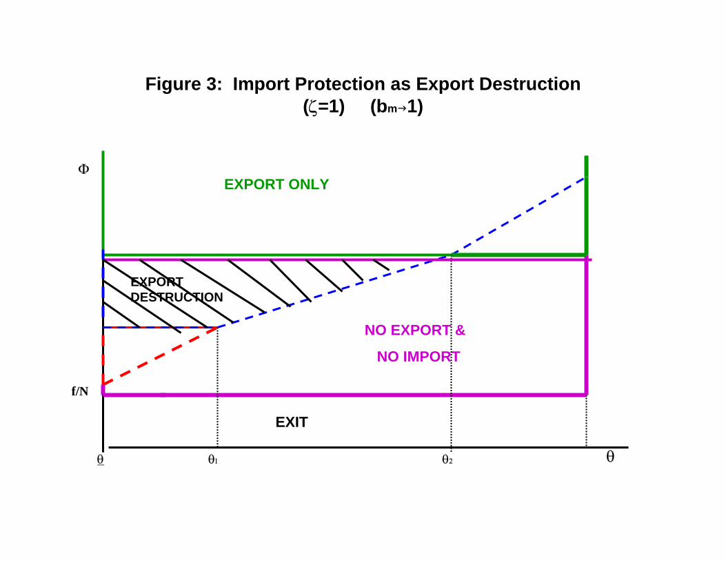
Figure 3: Import Protection as Export Destruction(ζ=1) (bm 1)
NO EXPORT &
NO IMPORT
θ
Φ
f/N
θ1 θ2
EXIT
θ
EXPORT ONLY
EXPORT DESTRUCTION

Figure 4: Revenue and Profit Comparisons(Medium ε)
TRADE
AUT
φ*A φ*T
r(φ,d)
(0,0) (1,1) φ
π(φ,d)
φ∗A φ∗T (0,0) (1,1) φ
TRADEAUT

Figure 5: Revenue and Profit Comparisons(Low ε) (Firms which only import lose market share)
TRADE
AUT
φ*A φ*T
r(φ,d)
(0,0) φ
π(φ,d)
φ∗A φ*T (0,0) (1,1) φ
TRADEAUT
(0,1) (1,1) (0,1)
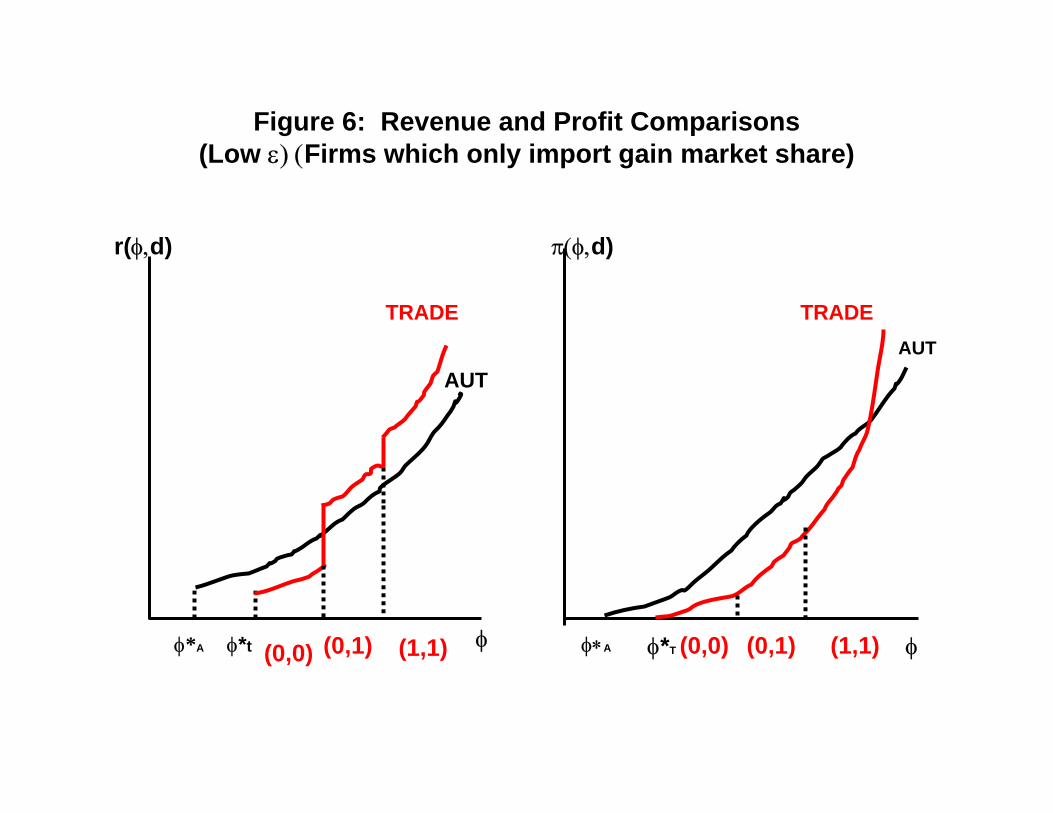
Figure 6: Revenue and Profit Comparisons(Low ε) (Firms which only import gain market share)
TRADE
AUT
φ*A φ*t
r(φ,d)
(0,0) φ
π(φ,d)
φ∗A φ*T (0,0) (1,1) φ
TRADEAUT
(0,1) (0,1)(1,1)
Recommended