
Imbens/Wooldridge, Lecture Notes 9, Summer ’07 1
What’s New in Econometrics NBER, Summer 2007
Lecture 9, Tuesday, July 31th, 3.15-4.15pm
Partial Identification
1. Introduction
Traditionally in constructing statistical or econometric models researchers look for models
that are (point-)identified: given a large (infinite) data set, one can infer without uncertainty
what the values are of the objects of interest, the estimands. Even though the fact that a
model is identified does not necessarily imply that we do well in finite samples, it would
appear that a model where we cannot learn the parameter values even in infinitely large
samples would not be very useful. Traditionally therefore researchers have stayed away from
models that are not (point-)identified, often adding assumptions beyond those that could
be justified using substantive arguments. However, it turns out that even in cases where
we cannot learn the value of the estimand exactly in large samples, in many cases we can
still learn a fair amount, even in finite samples. A research agenda initiated by Manski
(an early paper is Manski (1990), monographs include Manski (1995, 2003)), referred to as
partial identification, or earlier as bounds, and more recently adopted by a large number
of others, notably Tamer in a series papers (Haile and Tamer, 2003, Ciliberto and Tamer,
2007; Aradillas-Lopez and Tamer, 2007), has taken this perspective. In this lecture we focus
primarily on a number of examples to show the richness of this approach. In addition we
discuss some of the theoretical issues connected with this literature, and some practical issues
in implementation of these methods.
The basic set up we adopt is one where we have a random sample of units from some
population. For the typical unit, unit i, we observe the value of a vector of variables Zi.
Sometimes it is useful to think of there being in the background a latent variable variable
Wi. We are interested in some functional θ of the joint distribution of Zi and Wi, but, not
observing Wi for any units, we may not be able to learn the value of θ even in infinite samples
because the estimand cannot be written as a functional of the distribution of Zi alone. The

Imbens/Wooldridge, Lecture Notes 9, Summer ’07 2
three key questions are (i) what we can learn about θ in large samples (identification), (ii)
how do we estimate this (estimation), and (iii) how do we quantify the uncertainty regarding
θ (inference).
The solution to the first question will typically be a set, the identified set. Even if we
can characterize estimators for these sets, computing them can present serious challenges.
Finally, inference involves challenges concerning uniformity of the coverage rates, as well as
the question whether we are interested in coverage of the entire identified set or only of the
parameter of interest.
There are a number of cases of general interest. I will discuss two leading cases in more
detail. In the first case the focus is on a scalar, with the identified set equal to an interval with
lower and upper bound a smooth,√N -estimable functional of the data. A second case of
interest is that where the information about the parameters can be characterized by moment
restrictions, often arising from revealed preference comparisons between utilities at actions
taken and actions not taken. I refer to this as the generalized inequality restrictions (GIR)
setting. This set up is closely related to the generalized method of moments framework.
2. Partial Identification: Examples
Here we discuss a number of examples to demonstrate the richness of the partial identi-
fication approach.
2.1 Missing Data
This is a basic example, see e.g., Manski (1990), and Imbens and Manski (2004). It is
substantively not very interesting, but it illustrates a lot of the basic issues. Suppose the
observed variable is the pair Zi = (Di, Di ·Yi), and the unobserved variable is Wi = Yi. Di is
a binary variable. This corresponds to a missing data case. If Di = 1, we observe Yi, and if
Di = 0 we do not observe Yi. We always observe the missing data indicator Di. We assume
the quantity of interest is the population mean θ = E[Yi].
In large samples we can learn p = E[Di] and µ1 = E[Yi|Di = 1]. The data contain no

Imbens/Wooldridge, Lecture Notes 9, Summer ’07 3
information about µ0 = E[Yi|Di = 0]. It can be useful, though not always possible, to write
the estimand in terms of parameters that are point-identified and parameters that the data
are not informative about. In this case we can do so:
θ = p · µ1 + (1 − p) · µ0.
Since even in large samples we learn nothing about µ0, it follows that without additional
information there is no limit on the range of possible values for θ. Even if p is very close to
1, this small probability that Di = 0 combined with the possibility that µ0 is very large or
very small allows for a wide range of values for θ.
Now suppose we know that the variable of interest is binary: Yi ∈ {0, 1}. Then natural
(not data-informed) lower and upper bounds for µ0 are 0 and 1 respectively. This implies
bounds on θ:
θ ∈ [θLB, θUB] = [p · µ1, p · µ1 + (1 − p)] .
These bounds are sharp, in the sense that without additional information we can not improve
on them. Formally, for all values θ in [θLB, θUB], we can find a joint distribution of (Yi,Wi)
that is consistent with the joint distribution of the observed data and with θ. Even if Y is
not binary, but has some natural bounds, we can obtain potentially informative bounds on
θ.
We can also obtain informative bounds if we modify the object of interest a little bit.
Suppose we are interested in quantiles of the distribution of Yi. To make this specific,
suppose we are interested in the median of Yi, θ0.5 = med(Yi). The largest possible value
for the median arises if all the missing value of Yi are large. Define qτ(Yi|Di = d) to be the
τ quantile of the conditional distribution of Yi given Di = d. Then the median cannot be
larger than q1/(2p)(Yi|Di = 1) because even if all the missing values were large, we know that
at least p · (1/(2p)) = 1/2 of the units have a value less than or equal to q1/(2p)(Yi|Di = 1).
Similarly, the smallest possible value for the median corrresponds to the case where all the

Imbens/Wooldridge, Lecture Notes 9, Summer ’07 4
missing values are small, leading to a lower bound of q(2p−1)/(2p)(Yi|Di = 1). Then, if p > 1/2,
we can infer that the median must satisfy
θ0.5 ∈ [θLB, θUB] =[
q(2p−1)/(2p)(Yi|Di = 1), q1/(2p)(Yi|Di = 1)]
,
and we end up with a well defined, and, depending on the data, more or less informative
identified interval for the median. If fewer than 50% of the values are observed, or p < 1/2,
then we cannot learn anything about the median of Yi without additional information (for
example, a bound on the values of Yi), and the interval is (−∞,∞). More generally, we can
obtain bounds on the τ quantile of the distribution of Yi, equal to
θτ ∈ [θLB, θUB] =[
q(τ−(1−p))/p(Yi|Di = 1), qτ/p(Yi|Di = 1)]
.
which is bounded if the probability of Yi being missing is less than min(τ, 1 − τ ).
2.2 Returns to Schooling
Manski and Pepper (2000, MP) are interested in estimating returns to schooling. They
start with an individual level response function Yi(w), where w ∈ {0, 1, . . . , 20} is years of
schooling. Let
∆(s, t) = E[Yi(t)− Yi(s)],
be the difference in average outcomes (log earnings) given t rather than s years of schooling.
Values of ∆(s, t) at different combinations of (s, t) are the object of interest. Let Wi be
the actual years of school, and Yi = Yi(Wi) be the actual log earnings. If one makes an
unconfoundedness type assumption that
Yi(w) ⊥⊥ Wi
∣
∣
∣ Xi,
for some set of covariates, one can estimate ∆(s, t) consistently given some support con-
ditions. MP relax this assumption. Dropping this assumption entirely without additional
Imbens/Wooldridge, Lecture Notes 9, Summer ’07 5
assumptions one can derive the bounds using the missing data results in the previous sec-
tion. In this case most of the data would be missing, and the bounds would be wide. More
interestingly MP focus on a number of alternative, weaker assumptions, that do not allow
for point-identification of ∆(s, t), but that nevertheless may be able to narrow the range of
values consistent with the data to an informative set. One of their assumptions requires that
increasing education does not lower earnings:
Assumption 1 (Monotone Treatment Response)
If w′ ≥ w, then Yi(w′) ≥ Yi(w).
Another assumption states that, on average, individuals who choose higher levels of education
would have higher earnings at each level of education than individuals who choose lower levels
of education.
Assumption 2 (Monotone Treatment Selection)
If w′′ ≥ w′, then for all w, E[Yi(w)|Wi = w′′] ≥ E[Yi(w)|Wi = w′].
Both assumptions are consistent with many models of human capital accumulation. They
also address the main concern with the exogenous schooling assumption, namely that higher
ability individuals who would have had higher earnings in the absence of more schooling, are
more likely to acquire more schooling.
Under these two assumptions, the bound on the average outcome given w years of school-
ing is
E[Yi|Wi = w] · Pr(Wi ≥ w) +∑
v<w
E[Yi|Wi = v] · Pr(Wi = v)
≤ E[Yi(w)] ≤
E[Yi|Wi = w] · Pr(Wi ≤ w) +∑
v>w
E[Yi|Wi = v] · Pr(Wi = v).

Imbens/Wooldridge, Lecture Notes 9, Summer ’07 6
Using data from the National Longitudinal Study of Youth MP a point estimator for the
upper bound on the the returns to four years of college, ∆(12, 16) to be 0.397, with a 0.95
upper quantile of 0.450. Translated into an average yearl returns this gives us 0.099, which
is in fact lower than some estimates that have been reported in the literature. This analysis
suggests that the upper bound is in this case reasonably informative, given a remarkably
weaker set of assumptions.
2.3 Changes in Inequality and Selection
There is a large literature on the changes in the wage distribution and the role of changes
in the returns to skills that drive these changes. One concern is that if one compares the
wage distribution at two points in time, any differences may be partly or wholly due to
differences in the composition of the workforce. Blundell, Gosling, Ichimura, and Meghir
(2007, BGHM) investigate this using bounds. They study changes in the wage distribution
in the United Kingdom for both men and women. Even for men at prime employment ages
employment in the late nineties is less than 0.90, down from 0.95 in the late seventies. The
concern is that the 10% who do not work are potentially different, both from those who work,
as well as from those who did not work in the seventies, corrupting comparisons between
the wage distributions in both years. Traditionally such concerns may have been ignored by
implicitly assuming that the wages for those not working are similar to those who are working,
possibly conditional on some observed covariates, or they may have been addressed by using
selection models. The type of selection models used ranges from very parametric models of
the type originally developed by Heckman (1978), to semi- and non-parametric versions of
this (Heckman, 1990). The concern that BGHM raise is that those selection models rely on
assumptions that are difficult to motivate by economic theory. They investigate what can
be learned about the changes in the wage distributions without the final, most controversial
assumptions of those selection models.
BGHM focus on the interquartile range as their measure of dispersion in the wage dis-
tribution. As discussed in Section 2.1, this is convenient, because bounds on quantiles often
exist in the presence of missing data. Let FY |X(y|x) be the distribution of wages condi-

Imbens/Wooldridge, Lecture Notes 9, Summer ’07 7
tional on some characteristics X. This is assumed to be well defined irrespective of whether
an individual works or not. However, if an individual does not work, Yi is not observed.
Let Di be an indicator for employment. Then we can estimate the conditional wage dis-
tribution given employment, FY |X,D(y|x, d = 1), as well as the probability of employment,
p(x) = pr(Di = 1|Xi = x). This gives us tight bounds on the (unconditional on employment)
wage distribution
FY |X,D(y|x, d = 1) · p(x) ≤ FY |X,D(y|x, d = 1) ≤ FY |X,D(y|x, d = 1) · p(x) + (1 − p(x)).
We can convert this to bounds on the τ quantile of the conditional distribution of Yi given
Xi = x, denoted by qτ(x):
q(τ−(1−p(x)))/p(x)(Yi|Di = 1) ≤ qτ (x) ≤ qτ/p(x)(Yi|Di = 1),
Then this can be used to derive bounds on the interquartile range q0.75(x)− q0.25(x):
q(0.75−(1−p(x)))/p(x)(Yi|Di = 1) − q0.25/p(x)(Yi|Di = 1)
≤ q0.75(x) − q0.25(x) ≤
q(0.25−(1−p(x)))/p(x)(Yi|Di = 1) − q0.75/p(x)(Yi|Di = 1).
So far this is just an application of the missing data bounds derived in the previous
section. What makes this more interesting is the use of additional information short of
imposing a full selection model that would point identify the interquartile range. The first
assumption BGHM add is that of stochastic dominance of the wage distribution for employed
individuals:
FY |X,D(y|x, d = 1) ≤ FY |X,D(y|x, d = 0).

Imbens/Wooldridge, Lecture Notes 9, Summer ’07 8
One can argue with this stochastic dominance assumption, but within groups homogenous
in background characteristics including education, it may be reasonable. This assumption
tightens the bounds on the distribution function to:
FY |X,D(y|x, d = 1) ≤ FY |X,D(y|x, d = 1) ≤
FY |X,D(y|x, d = 1) · p(x) + (1 − p(x)).
Another assumption BGHM consider is a modification of an instrumental variables as-
sumption that an observed covariate Z is excluded from the wage distribution:
FY |X,Z(y|X = x, Z = z) = FY |X,Z(y|X = x, Z = z′), for all x, z, z′.
This changes the bounds on the distribution function to:
maxzFY |X,Z,D(y|x, z, d = 1) · p(x, z)
≤ FY |X,D(y|x) ≤
minzFY |X,Z,D(y|x, z, d = 1) · p(x) + (1 − p(x)).
(An alternative weakening of the standard instrumental variables assumption is in Hotz,
Mullin and Sanders (1997), where a valid instrument exists, but is not observed directly.)
Such an instrument may be difficult to find, and BGHM argue that it may be easier
to find a covariate that affects the wage distribution in one direction, using a monotone
instrumental variables restriction suggested by Manski and Pepper (2000):
FY |X,Z(y|X = x, Z = z) ≤ FY |X,Z(y|X = x, Z = z′), for all x, z < z′.
This discussion is somewhat typical of what is done in empirical work in this area. A
number of assumptions are considered, with the implications for the bounds investigated.
The results lay out part of the mapping between the assumptions and the bounds.
Imbens/Wooldridge, Lecture Notes 9, Summer ’07 9
2.4 Random Effects Panel Data Models with Initial Condition Problems
Honore and Tamer (2006) study dynamic random effects panel data models. We observe
(Xi1, Yi1, . . . , XiT , YiT ), for i = 1, . . . , N . The time dimension T is small relative to the
cross-section dimension N . Large sample approximations are based on fixed T and large
N . Inference would be standard if we specified a parametric model for the (components of
the) conditional distribution of (Yi1, . . . , YiT ) given (Xi1, . . . , XiT ). In that case we could use
maximum likelihood methods. However, it is difficult to specify this conditional distribution
directly. Often we start with a model for the evolution of Yit in terms of the present and
past covariates and its lags. As an example, consider the model
Yit = 1{X ′itβ + Yit−1γ + αi + εit ≥ 0},
with the εit independent over time and individuals, and normally distributed, εit ∼ N (0, 1).
The object of interest is the parameter governing the dynamics, γ. This model gives us the
conditional distribution of Yi2, . . . , YiT given Yi1, αi and given Xi1, . . . , XiT . Suppose we also
postulate a parametric model for the random effects αi:
α|Xi1, . . . , XiT ∼ G(α|θ),
(so in this case αi is independent of the covariates). Then the model is (almost) complete, in
the sense that we can almost write down the conditional distribution of (Yi1, . . . , YiT ) given
(Xi1, . . . , XiT ). All that is missing is the conditional distribution of the initial condition:
p(Yi1|αi, Xi1, . . . , XiT ).
This is a difficult distribution to specify. One could directly specify this distribution, but
one might want it to be internally consistent across different number of time periods, and
that makes it awkward to choose a functional form. See for general discussions of this initial
conditions problem Wooldridge (2002). Honore and Tamer investigate what can be learned
about γ without making parametric assumptions about this distribution. From the literature

Imbens/Wooldridge, Lecture Notes 9, Summer ’07 10
it is known that in many cases γ is not point-identified (for example, the case with T ≤ 3,
no covariates, and a logistic distribution for εit). Nevertheless, it may be that the range of
values of γ consistent with the data is very small, and it might reveal the sign of γ.
Honore and Tamer study the case with a discrete distribution for α, with a finite and
known set of support points. They fix the support to be −3,−2.8, . . . , 2.8, 3, with unknown
probabilities. Given that the εit are standard normal, this is very flexible. In a computational
exercise they assume that the true probabilities make this discrete distribution mimic the
standard normal distribution. In addition they set Pr(Yi1 = 1|αi) = 1/2. In the case with
T = 3 they find that the range of values for γ consistent with the data generating process
(the identified set) is very narrow. If γ is in fact equal to zero, the width of the set is zero.
If the true value is γ = 1, then the width of the interval is approximately 0.1. (It is largest
for γ close to, but not equal to, -1.) See Figure 1, taken from Honore and Tamer (2006).
The Honore-Tamer analysis, in the context of the literature on initial conditions problems,
shows very nicely the power of the partial identification approach. A problem that had been
viewed as essentially intractable, with many non-identification results, was shown to admit
potentially precise inferences despite these non-identification results.
2.5 Auction Data
Haile and Tamer (2003, HT from hereon), in what is one of the most influential appli-
cations of the partial identification approach, study English or oral ascending bid auctions.
In such auctions bidders offer increasingly higher prices until only one bidder remains. HT
focus on a symmetric independent private values model. In auction t, for t = 1, . . . , T , bid-
der i has a value νit, drawn independently from the value for bidder j. Large sample results
refer to the number of auctions getting large. HT assume that the value distribution is the
same in each auction (after adjusting for observable auction characteristics). A key object of
interest, is the value distribution. Given that one can derive other interesting objects, such
as the optimal reserve price.
One can imagine a set up where the researcher observes, as the price increases, for each
Imbens/Wooldridge, Lecture Notes 9, Summer ’07 11
bidder whether that bidder is still participating in the auction. (Milgrom and Weber (1982)
assume that each bidder continuously confirms their participation by holding down a button
while prices rise continuously.) In that case one would be able to infer for each bidder their
valuation, and thus directly estimate the value distribution.
This is not what is typically observed. Instead of prices rising continuously, there are
jumps in the bids, and for each bidder we do not know at any point in time whether they are
still participating unless they subsequently make a higher bid. HT study identification in
this, more realistic, setting. They assume that no bidder ever bids more than their valuation,
and that no bidder will walk away and let another bidder win the auction if the winning
bid is lower than their own valuation. Under those two assumptions, HT show that one can
derive bounds on the value distribution.
One set of bounds they propose is as follows. Let the highest bid for participant i in
auction t be bit. The number of participants in auction t is nt. Ignoring any covariates,
let the distribution of the value for individual i, νit, be Fν(v). This distribution function is
the same for all auctions. Let Fb(b) = Pr(bit ≤ b) be the distribution function of the bids
(ignoring variation in the number of bidders by auction). This distribution can be estimated
because the bids are observed. The winning bid in auction t is Bt = maxi=1,...,ntbit. First
HT derive an upper bound on the distribution function Fν(v). Because no bidder ever bids
more than their value, it follows that bit ≤ νit. Hence, without additional assumptions,
Fν(v) ≤ Fb(v), for all v.
For a lower bound on the distribution function one can use the fact that the second
highest of the values among the n participants in auction t must be less than or equal to the
winning bid. This follows from the assumption that no participant will let someone else win
with a bid below their valuation. Let Fν,m:n(v) denote the mth order statistic in a random
sample of size n from the value distribution, and let FB,n:n(b) denote the distribution of the

Imbens/Wooldridge, Lecture Notes 9, Summer ’07 12
winning bid in auctions with n participants. Then
FB,n:n(v) ≤ Fν,n−1:n(v).
The distribution of the any order statistic is monotonically related to the distribution of the
parent distribution, and so a lower bound on Fν,n−1:n(v) implies a lower bound on Fν(v).
HT derive tighter bounds based on the information in other bids and the inequalities
arising from the order statistics, but the above discussion illustrates the point that outside
of the Milgrom-Weber button auction model one can still derive bounds on the value dis-
tribution in an English auction even if one cannot point-identify the value distribution. If
in fact the highest bid for each individual was equal to their value (other than for the win-
ner for whom the bid is equal to the second highest value), the bounds would collaps and
point-identification would be obtained.
2.6 Entry Models and Inequality Conditions
Recently a number of papers has studied entry models in settings with multiple equilibria.
In such settings traditionally researchers have added ad hoc equilbrium selection mechanisms.
In the recent literature a key feature is the avoidance of such assumptions, as these are often
difficult to justify on theoretical grounds. Instead the focus is on what can be learned in the
absence of such assumptions. In this section I will discuss some examples from this literature.
An important feature of these models is that they often lead to inequality restrictions, where
the parameters of interest θ satisfy
E[ψ(Z, θ)] ≥ 0,
for known ψ(z, θ). This relates closely to the standard (Hansen, 1983) generalized method of
moments (GMM) set up where the functions ψ(Z, θ) would have expectation equal to zero at
the true values of the parameters. We refer to this as the generalized inequality restrictions
(GIR) form. These papers include Pakes, Porter, Ho, and Ishii (2006), Cilberto and Tamer
(2004, CM from hereon), Andrews, Berry and Jia (2004). Here I will discuss a simplified

Imbens/Wooldridge, Lecture Notes 9, Summer ’07 13
version of the CM model. Suppose two firms, A and B, contest a set of markets. In market
m, m = 1, . . . ,M , the profits for firms A and B are
πAm = αA + δA · dBm + εAm, and πBm = αB + δB · dAm + εBm.
where dFm = 1 if firm F is present in market m, for F ∈ {A,B}, and zero otherwise. The
more realistic model CM consider also includes observed market and firm characteristics.
Firms enter market m if their profits in that market are positive. Firms observe all compo-
nents of profits, including those that are unobserved to the econometrician, (εAm, εBm), and
so their decisions satisfy:
dAm = 1{πAm ≥ 0}, dBm = 1{πBm ≥ 0}. (1)
(Pakes, Porter, Ho, and Ishii allow for incomplete information where expected profits are
at least as high for the action taken as for actions not taken, given some information set.)
The unobserved (to the econometrician) components of profits, εFm, are independent accross
markets and firms. For ease of exposition we assume here that they have a normal N (0, 1)
distribution. (Note that we only observe indicators of the sign of profits, so the scale of
the unobserved components is not relevant for predictions.) The econometrician observes in
each market only the pair of indicators dA and dB . We focus on the case where the effect of
entry of the other firm on a firm’s profits, captured by the parameters δA and δB is negative,
which is the case of most economic interest.
An important feature of this model is that given the parameters θ = (αA, δA, αB, δB), for
a given set of (εAm, εBm) there is not necessarily a unique solution (dAm, dBm). For pairs of
values (εAm, εBm) such that
−αA < εA ≤ −αA − δA, −αB < εB ≤ −αB − δB,
both (dA, dB) = (0, 1) and (dA, dB) = (1, 0) satisfy the profit maximization condition (1).
In the terminology of this literature, the model is not complete. It does not specify the

Imbens/Wooldridge, Lecture Notes 9, Summer ’07 14
outcomes given the inputs. Figure 1, adapted from CM, shows the different regions in the
(εAm, εBm) space.
The implication of this is that the probability of the outcome (dAm, dBm) = (0, 1) cannot
be written as a function of the parameters of the model, θ = (αA, δA, αB, δB), even given
distributional assumptions on (εAm, εBm). Instead the model implies a lower and upper
bound on this probability:
HL,01(θ) ≤ Pr ((dAm, dBm) = (0, 1)) ≤ HU,01(θ).
Inspecting Figure 1 shows that
HL,01(θ) = Pr(εAm < −αA,−αB < εBm)
+Pr(−αA ≤ εAm < −αA − δA,−αB − δB < εBm),
and
HU,01(θ) = Pr(εAm < −αA, αB < εBm)
+Pr(−αA ≤ εAm < −αA − δA,−αB − δB < εBm),
+Pr(−αA ≤ εAm < −αA − δA,−αB < εBm < −αB − δB),
Similar expressions can be derived for the probability Pr ((dAm, dBm) = (1, 0)). Thus in
general we can write the information about the parameters in large samples as
HL,00(θ)HL,01(θ)HL,10(θ)HL,11(θ)
≤
Pr ((dAm, dBm) = (0, 0))Pr ((dAm, dBm) = (0, 1))Pr ((dAm, dBm) = (1, 0))Pr ((dAm, dBm) = (1, 1))
≤
HU,00(θ)HU,01(θ)HU,11(θ)HU,11(θ)
.
(For (dA, dB) = (0, 0) or (dA, dB) = (1, 1) the lower and upper bound coincide, but for ease
of exposition we treat all four configurations symmetrically.) The HL,ij(θ) and HU,ij(θ) are

Imbens/Wooldridge, Lecture Notes 9, Summer ’07 15
known functions of θ. The data allow us to estimate the foru probabilities, which contain
only three separate pieces of information because the probabilities add up to one. Given
these probabilities, the identified set is the set of all θ that satisfy all eight inequalities. In
the simple model above, there are four parameters. Even in the case with the lower and
upper bounds for the probabilities coinciding, these would in general not be identified.
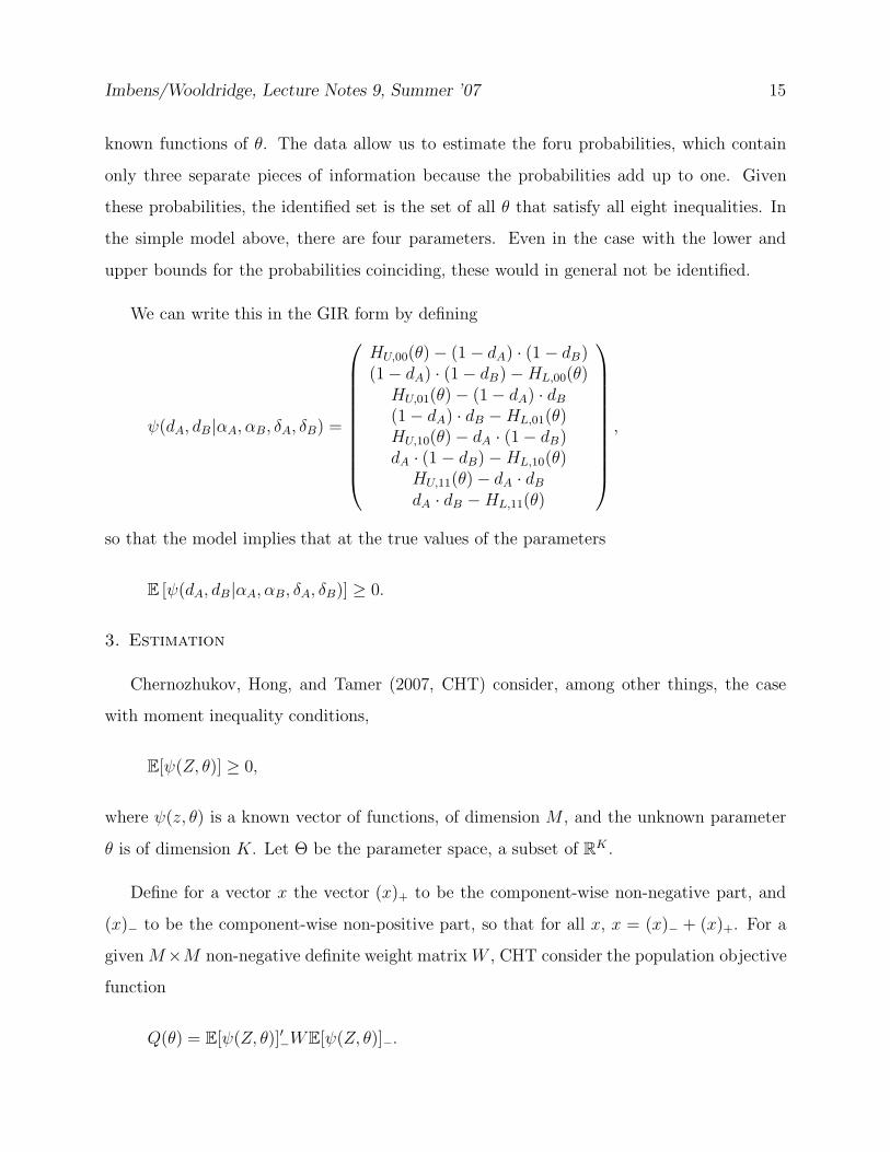
We can write this in the GIR form by defining
ψ(dA, dB |αA, αB, δA, δB) =
HU,00(θ) − (1 − dA) · (1 − dB)(1 − dA) · (1 − dB) −HL,00(θ)HU,01(θ) − (1 − dA) · dB
(1 − dA) · dB −HL,01(θ)HU,10(θ) − dA · (1 − dB)dA · (1 − dB) −HL,10(θ)HU,11(θ) − dA · dB
dA · dB −HL,11(θ)
,
so that the model implies that at the true values of the parameters
E [ψ(dA, dB |αA, αB, δA, δB)] ≥ 0.
3. Estimation
Chernozhukov, Hong, and Tamer (2007, CHT) consider, among other things, the case
with moment inequality conditions,
E[ψ(Z, θ)] ≥ 0,
where ψ(z, θ) is a known vector of functions, of dimension M , and the unknown parameter
θ is of dimension K. Let Θ be the parameter space, a subset of RK .
Define for a vector x the vector (x)+ to be the component-wise non-negative part, and
(x)− to be the component-wise non-positive part, so that for all x, x = (x)− + (x)+. For a
givenM×M non-negative definite weight matrix W , CHT consider the population objective
function
Q(θ) = E[ψ(Z, θ)]′−WE[ψ(Z, θ)]−.
Imbens/Wooldridge, Lecture Notes 9, Summer ’07 16
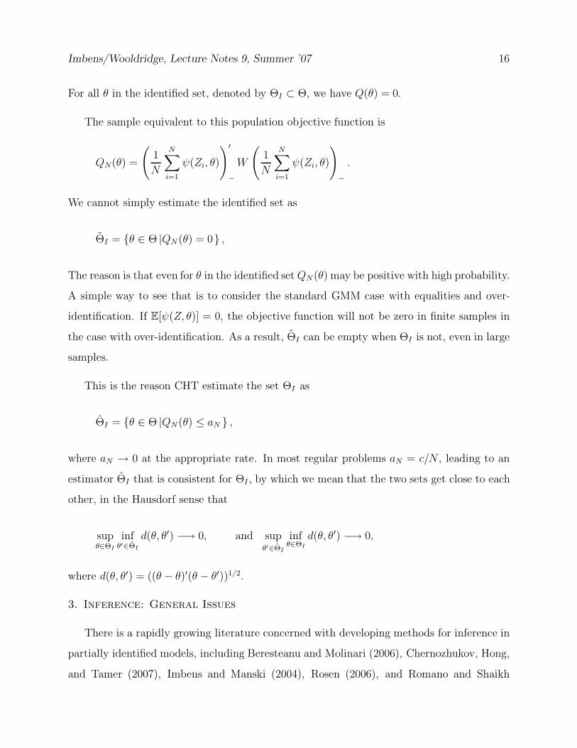
For all θ in the identified set, denoted by ΘI ⊂ Θ, we have Q(θ) = 0.
The sample equivalent to this population objective function is
QN(θ) =
(
1
N
N∑
i=1
ψ(Zi, θ)
)′
−
W
(
1
N
N∑
i=1
ψ(Zi, θ)
)
−
.
We cannot simply estimate the identified set as
ΘI = {θ ∈ Θ |QN (θ) = 0} ,
The reason is that even for θ in the identified setQN (θ) may be positive with high probability.
A simple way to see that is to consider the standard GMM case with equalities and over-
identification. If E[ψ(Z, θ)] = 0, the objective function will not be zero in finite samples in
the case with over-identification. As a result, ΘI can be empty when ΘI is not, even in large
samples.
This is the reason CHT estimate the set ΘI as
ΘI = {θ ∈ Θ |QN (θ) ≤ aN } ,
where aN → 0 at the appropriate rate. In most regular problems aN = c/N , leading to an
estimator ΘI that is consistent for ΘI , by which we mean that the two sets get close to each
other, in the Hausdorf sense that
supθ∈ΘI
infθ′∈ΘI
d(θ, θ′) −→ 0, and supθ′∈ΘI
infθ∈ΘI
d(θ, θ′) −→ 0,
where d(θ, θ′) = ((θ − θ)′(θ − θ′))1/2.
3. Inference: General Issues
There is a rapidly growing literature concerned with developing methods for inference in
partially identified models, including Beresteanu and Molinari (2006), Chernozhukov, Hong,
and Tamer (2007), Imbens and Manski (2004), Rosen (2006), and Romano and Shaikh

Imbens/Wooldridge, Lecture Notes 9, Summer ’07 17
(2007ab). In many cases the partially identified set itself is difficult to characterize. In the
scalar case this can be much simpler. There it often is an interval, [θLB, θUB]. There are by
now a number of proposals for constructing confidence sets. They differ in implementation
as well as in their goals. One issue is whether one wants a confidence set that includes
each element of the identified set with fixed probability, or the entire identified set with that
probability. Formally, the first question looks for a confidence set CIθα that satisfies
infθ∈[θLB,θUB]
Pr(
θ ∈ CIθα
)
≥ α.
In the second case we look for a set CI[θLB,θUB]α such that
Pr(
[θLB, θUB] ⊂ CIθα)
≥ α.
The second requirement is stronger than the first, and so generally CIθα ⊂ CI[θLB,θUB]
α . Here
we follow Imbens and Manski (2004) and Romano and Shaikh (2007a) who focus on the
first case. This seems more in line with teh traditional view of confidence interval in that
they should cover the true value of the parameter with fixed probability. It is not clear why
the fact that the object of interest is not point-identified should change the definition of a
confidence interval. CHT and Romano and Shaikh (2007b) focus on the second case.
Next we discuss two specific examples to illustrate some of the issues that can arise, in
particular the uniformity of confidence intervals.
3.1 Inference: A Missing Data Problem
Here we continue the missing data example from Section 2.1. We have a random sample
of (Wi,Wi · Yi), for i = 1, . . . , N . Yi is known to lie in the interval [0, 1], interest is in
θ = E[Y ], and the parameter space is Θ = [0, 1]. Define µ1 = E[Y |W = 1], λ = E[Y |W = 0],
σ2 = V(Y |W = 1), and p = E[W ]. For ease of exposition we assume p is known. The
identified set is
ΘI = [p · µ1, p · µ1 + (1 − p)].

Imbens/Wooldridge, Lecture Notes 9, Summer ’07 18
Imbens and Manski (2004) discuss confidence intervals for this case. The key feature of this
problem, and similar ones, is that the lower and upper bounds are well-behaved functionals
of the joint distribution of the data that can be estimated at the standard parametric√N
rate with an asymptotic normal distribution. In this specific example the lower and upper
bound are both functions of a single unknown parameter, the conditional mean µ1. The first
step is a 95% confidence interval for µ1. Let N1 =∑
i Wi and Y 1 =∑
iWi · Yi/N1. The
standard confidence interval is
CIµ1
α =[
Y − 1.96 · σ/√N1, Y + 1.96 · σ/
√N1
]
.
Consider the confidence interval for the lower and upper bound:
CIp·µ1
α =[
p ·(
Y − 1.96 · σ/√N 1
)
, p ·(
Y + 1.96 · σ/√N1
)]
,
and
CIp·µ1+(1−p)α =
[
p ·(
Y − 1.96 · σ/√N1
)
+ (1 − p), p ·(
Y + 1.96 · σ/√N1
)
+ 1 − p]
.
A simple and valid confidence interval can be based on the lower confidence bound on the
lower bound and the upper confidence bound on the upper bound:
CIθα =
[
p ·(
Y − 1.96 · σ/√N1
)
, p ·(
Y + 1.96 · σ/√N 1
)
+ 1 − p]
.
This is generally conservative. For each θ in the interior of ΘI, the asymptotic coverage rate
is 1. For θ ∈ {θLB, θUB}, the coverage rate is α + (1 − α)/2.
The interval can be modified to give asymptotic coverage equal to α by changing the
quantiles used in the confidence interval construction, essentially using one-sided critical
values,
CIθα =
[
p ·(
Y − 1.645 · σ/√N 1
)
, p ·(
Y + 1.645 · σ/√N1
)
+ 1 − p]
.

Imbens/Wooldridge, Lecture Notes 9, Summer ’07 19
This has the problem that if p = 0 (when θ is point-identified), the coverage is only α−(1−α).
In fact, for values of p close to zero, the confidence interval would be shorter than the
confidence interval in the point-identified case. Imbens and Manski (2004) suggest modifying
the confidence interval to
CIθα =
[
p ·(
Y − CN · σ/√N1
)
, p ·(
Y + CN · σ/√N1
)
+ 1 − p]
,
where the critical value CN satisfies
Φ
(
CN +√N · 1 − p
σ/√p
)
− Φ(−CN ) = α.
and CN = 1.96 if p = 0. This confidence interval has asymptotic coverage 0.95, uniformly
over p.
3.2. Inference: Multiple Inequalities
Here we look at inference in the Genereralized Inequality (GIR) setting. The example is
a simplified version of the moment inequality type of problems discussed in CHT, Romano
and Shaikh (2007ab), Pakes, Porter, Ho, and Ishii (2006), and Andrews and Guggenberger
(2007). Suppose we have two moment inequalities,
E[X] ≥ θ, and E[Y ] ≥ θ.
The parameter space is Θ = [0,∞). Let µX = E[X], and µY = E[Y ]. We have a random
sample of size N of the pairs (X, Y ). The identified set is
ΘI = [0,min(µX , µY )].
The key difference with the previous example is that the upper bound is no longer a
smooth, well-behaved functional of the joint distribution. In the simple two-inequality ex-
ample, if µX is close to µY , the distribution of the estimator for the upper bound is not well
approximated by a normal distribution. Suppose we estimate the means of X and Y by

Imbens/Wooldridge, Lecture Notes 9, Summer ’07 20
X, and Y , and that the variances of X and Y are known to be equal to σ2. A naive 95%
confidence interval would be
Cθα = [0,min(X, Y ) + 1.645 · σ/N ].
This confidence interval essentially ignores the moment inequality that is not binding in the
sample. It has asymptotic 95% coverage for all values of µX , µY , as long as min(µX , µY ) > 0,
and µX 6= µY . The first condition (min(µX , µY ) > 0) is the same as the condition in the
Imbens-Manski example. It can be dealt with in the same way by adjusting the critical value
slightly based on an initial estimate of the width of the identified set.
The second condition raises a different uniformity concern. The naive confidence interval
essentially assumes that the researcher knows which moment conditions are binding. This is
true in large samples, unless there is a tie. However, in finite samples ignoring uncertainty
regarding the set of binding moment inequalities may lead to a poor approximation, especially
if there are many inequalities. One possibility is to construct conservative confidence intervals
(e.g., Pakes, Porter, Ho, and Ishii, 2007). However, such intervals can be unnecessarily
conservative if there are moment inequalities that are far from binding.
One would like construct confidence intervals that asymptotically ignore irrelevant in-
equalities, and at the same time are valid uniformly over the parameter space. Bootstrap-
ping is unlikely to work in this setting. One way of obtaining confidence intervals that are
uniformly valid is based on subsampling. See Romano and Shaikh (2007a), and Andrews
and Guggenberger (2007). Little is known about finite sample properties in realistic settings.

Imbens/Wooldridge, Lecture Notes 9, Summer ’07 21
References
Andrews, D., S. Berry, and P. Jia (2004), “Confidence Regions for Parameters
in Discrete Games with Multiple Equilibria, with an Application to Discount Chain Store
Location,”unpublished manuscript, Department of Economics, Yale University.
Andrews, D., and P. Guggenberger (2004), “The Limit of Finite Sample Size
and a Problem with Subsampling,”unpublished manuscript, Department of Economics, Yale
University.
Aradillas-Lopez, A., and E. Tamer (2007), “The Identification Power of Equilib-
rium in Games,”unpublished manuscript, Department of Economics, Princeton University.
Balke, A., and J. Pearl, (1997), “Bounds on Treatment Effects from Studies with
Imperfect Compliance,”Journal of the American Statistical Association, 92: 1172-1176.
Beresteanu, A., and F. Molinari, (2006), “Asymptotic Properties for a Class of
Partially Identified Models,”Unpublished Manuscript, Department of Economics, Cornell
University.
Blundell, R., M. Browning, and I. Crawford, (2007), “Best Nonparametric
Bounds on Demand Responses,”Cemmap working paper CWP12/05, Department of Eco-
nomics, University College London.
Blundell, R., A. Gosling, H. Ichimura, and C. Meghir, (2007), “Changes in
the Distribution of Male and Female Wages Accounting for Employment Composition Using
Bounds,”Econometrica, 75(2): 323-363.
Chernozhukov, V., H. Hong, and E. Tamer (2007), “Estimation and Confidence
Regions for Parameter Sets in Econometric Models,”forthcoming, Econometrica.
Ciliberto, F., and E. Tamer (2004), “Market Structure and Multiple Equilibria in
Airline Markets,”Unpublished Manuscript.
Haile, P., and E. Tamer (2003), “Inference with an Incomplete Model of English
Auctions,”Journal of Political Economy, Vol 111(1), 1-51.
Heckman, J., (1978), “Dummy Endogenous Variables in a Simultaneous Equations

Imbens/Wooldridge, Lecture Notes 9, Summer ’07 22
System”, Econometrica, Vol. 46, 931–61.
Heckman, J. J. (1990), ”Varieties of Selection Bias,” American Economic Review 80,
313-318.
Honore, B., and E. Tamer (2006), “Bounds on Parameters in Dynamic Discrete
Choice Models,”Econometrica, 74(3): 611-629.
Hotz, J., C. Mullin, and S. Sanders, (1997), “Boudning Causal Effects Using Data
from a Contaminated Natural Experiment: Analysing the Effects of Teenage Childbearing,”
Review of Economic Studies, 64(4), 575-603.
Imbens, G., and C. Manski (2004), “Confidence Intervals for Partially Identified
Parameters,”Econometrica, 74(6): 1845-1857.
Manski, C., (1990), “Nonparametric Bounds on Treatment Effects,”American Economic
Review Papers and Proceedings, 80, 319-323.
Manski, C. (1995), Identification Problems in the Social Sciences, Cambridge, Harvard
University Press.
Manski, C. (2003), Partial Identification of Probability Distributions, New York: Springer-
Verlag.
Manski, C., and J. Pepper, (2000), “Monotone Instrumental Variables: With an
Application to the Returns to Schooling,”Econometrica, 68(): 997-1010.
Manski, C., G. Sandefur, S. McLanahan, and D. Powers (1992), “Alternative
Estimates of the Effect of Family Structure During Adolescence on High School,”Journal of
the American Statistical Association, 87(417):25-37.
Milgrom, P, and R. Weber (1982), “A Theory of Auctions and Competitive Bid-
ding,”Econometrica, 50(3): 1089-1122.
Pakes, A., J. Porter, K. Ho, and J. Ishii (2006), “Moment Inequalities and Their
Application,”Unpublished Manuscript.
Robins, J., (1989), “The Analysis of Randomized and Non-randomized AIDS Trials Us-
ing a New Approach to Causal Inference in Longitudinal Studies,”in Health Service Research
Imbens/Wooldridge, Lecture Notes 9, Summer ’07 23
Methodology: A Focus on AIDS, (Sechrest, Freeman, and Mulley eds), US Public Health
Service, 113-159.
Romano, J., and A. Shaikh (2006a), “Inference for Partially Identified Parame-
ters,”Unpublished Manuscript, Stanford University.
Romano, J., and A. Shaikh (2006b), “Inference for Partially Identified Sets,”Unpublished
Manuscript, Stanford University.
Rosen, A., (2005), “Confidence Sets for Partially Identified Parameters that Satisfy a Fi-
nite Number of Moment Inequalities,” Unpublished Manuscript, Department of Economics,
University College London.
Wooldridge, J (2002), “Simple Solutions to the Initial Conditions Problem in Dy-
namic, Nonlinear Panel Data Models with Unobserved Heterogeneity,”Journal of Applied
Econometrics, 20, 39-54.
Recommended