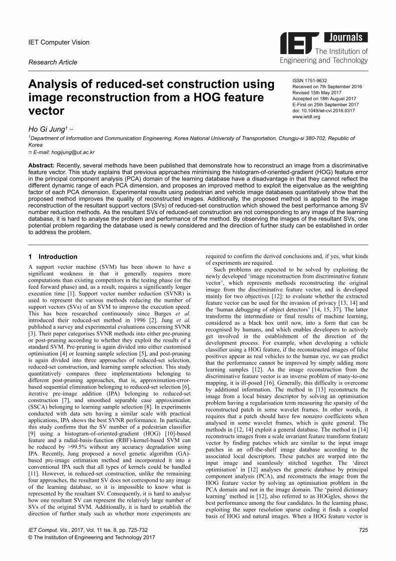
IET Computer Vision

Research Article

Analysis of reduced-set construction usingimage reconstruction from a HOG featurevector

ISSN 1751-9632Received on 7th September 2016Revised 15th May 2017Accepted on 18th August 2017E-First on 25th September 2017doi: 10.1049/iet-cvi.2016.0317www.ietdl.org

Ho Gi Jung1 1Department of Information and Communication Engineering, Korea National University of Transportation, Chungju-si 380-702, Republic ofKorea

E-mail: hogijung@ut.ac.kr

Abstract: Recently, several methods have been published that demonstrate how to reconstruct an image from a discriminativefeature vector. This study explains that previous approaches minimising the histogram-of-oriented-gradient (HOG) feature errorin the principal component analysis (PCA) domain of the learning database have a disadvantage in that they cannot reflect thedifferent dynamic range of each PCA dimension, and proposes an improved method to exploit the eigenvalue as the weightingfactor of each PCA dimension. Experimental results using pedestrian and vehicle image databases quantitatively show that theproposed method improves the quality of reconstructed images. Additionally, the proposed method is applied to the imagereconstruction of the resultant support vectors (SVs) of reduced-set construction which showed the best performance among SVnumber reduction methods. As the resultant SVs of reduced-set construction are not corresponding to any image of the learningdatabase, it is hard to analyse the problem and performance of the method. By observing the images of the resultant SVs, onepotential problem regarding the database used is newly considered and the direction of further study can be established in orderto address the problem.

1 IntroductionA support vector machine (SVM) has been shown to have asignificant weakness in that it generally requires morecomputations than existing competitors in the testing phase (or thefeed forward phase) and, as a result, requires a significantly longerexecution time [1]. Support vector number reduction (SVNR) isused to represent the various methods reducing the number ofsupport vectors (SVs) of an SVM to improve the execution speed.This has been researched continuously since Burges et al.introduced their reduced-set method in 1996 [2]. Jung et al.published a survey and experimental evaluations concerning SVNR[3]. Their paper categorises SVNR methods into either pre-pruningor post-pruning according to whether they exploit the results of astandard SVM. Pre-pruning is again divided into either customisedoptimisation [4] or learning sample selection [5], and post-pruningis again divided into three approaches of reduced-set selection,reduced-set construction, and learning sample selection. This studyquantitatively compares three implementations belonging todifferent post-pruning approaches, that is, approximation-error-based sequential elimination belonging to reduced-set selection [6],iterative pre-image addition (IPA) belonging to reduced-setconstruction [7], and smoothed separable case approximation(SSCA) belonging to learning sample selection [8]. In experimentsconducted with data sets having a similar scale with practicalapplications, IPA shows the best SVNR performance. In particular,this study confirms that the SV number of a pedestrian classifier[9] using a histogram-of-oriented-gradient (HOG) [10]-basedfeature and a radial-basis-function (RBF)-kernel-based SVM canbe reduced by >99.5% without any accuracy degradation usingIPA. Recently, Jung proposed a novel genetic algorithm (GA)-based pre-image estimation method and incorporated it into aconventional IPA such that all types of kernels could be handled[11]. However, in reduced-set construction, unlike the remainingfour approaches, the resultant SV does not correspond to any imageof the learning database, so it is impossible to know what isrepresented by the resultant SV. Consequently, it is hard to analysehow one resultant SV can represent the relatively large number ofSVs of the original SVM. Additionally, it is hard to establish thedirection of further study such as whether more experiments are

required to confirm the derived conclusions and, if yes, what kindsof experiments are required.

Such problems are expected to be solved by exploiting thenewly developed ‘image reconstruction from discriminative featurevector’, which represents methods reconstructing the originalimage from the discriminative feature vector, and is developedmainly for two objectives [12]: to evaluate whether the extractedfeature vector can be used for the invasion of privacy [13, 14] andthe ‘human debugging of object detectors’ [14, 15, 37]. The lattertransforms the intermediate or final results of machine learning,considered as a black box until now, into a form that can berecognised by humans, and which enables developers to activelyget involved in the establishment of the direction of thedevelopment process. For example, when developing a vehicleclassifier using a HOG feature, if the reconstructed images of falsepositives appear as real vehicles to the human eye, we can predictthat the performance cannot be improved by simply adding morelearning samples [12]. As the image reconstruction from thediscriminative feature vector is an inverse problem of many-to-onemapping, it is ill-posed [16]. Generally, this difficulty is overcomeby additional information. The method in [13] reconstructs theimage from a local binary descriptor by solving an optimisationproblem having a regularisation term measuring the sparsity of thereconstructed patch in some wavelet frames. In other words, itrequires that a patch should have few nonzero coefficients whenanalysed in some wavelet frames, which is quite general. Themethods in [12, 14] exploit a general database. The method in [14]reconstructs images from a scale invariant feature transform featurevector by finding patches which are similar to the input imagepatches in an off-the-shelf image database according to theassociated local descriptors. These patches are warped into theinput image and seamlessly stitched together. The ‘directoptimisation’ in [12] analyses the generic database by principalcomponent analysis (PCA), and reconstructs the image from theHOG feature vector by solving an optimisation problem in thePCA domain and not in the image domain. The ‘paired dictionarylearning’ method in [12], also referred to as HOGgles, shows thebest performance among the four candidates. In the learning phase,exploiting the super resolution sparse coding it finds a coupledbasis of HOG and natural images. When a HOG feature vector is

IET Comput. Vis., 2017, Vol. 11 Iss. 8, pp. 725-732© The Institution of Engineering and Technology 2017

725

given, it estimates the PCA coefficients common to both the imageand the HOG feature vector domain by projecting the HOG featurevector onto the HOG basis. Then, it reconstructs the original imageby summing the natural image basis multiplied by the coefficients.As methods exploiting the database show better image quality andthe problem at hand, i.e. image reconstruction from the resultantSV of the reduced-set construction, can generally use a learningdatabase, the approaches exploiting the database are selected.Among the methods belonging to these approaches, the method in[12] is preferred as it shows a clearer object contour than themethods in [14] in which edge information is distorted by the effectof stitching and blending.

This paper proposes an improvement of the ‘directoptimisation’ in [12], reconstructing the image by solvingoptimisation in the PCA domain, and shows that the proposedmethod is useful when developing reduced-set construction byanalysing the resultant SVs of the IPA in [3]. This study finds thatthe method minimising the HOG feature error in the PCA domainhas room for improvement as it ignores the different dynamic rangeof each dimension of the PCA domain. As a solution, this studyproposes a method weighing each dimension with its eigenvalue tocompensate for the different dynamic range and adopting a GAinstead of gradient-based optimisation to efficiently deal with adiscontinuous, non-linear and non-differentiable cost function.Experimental results with pedestrian and vehicle image databasesconfirm that the proposed method shows better performance thanthe HOGgles. By applying the proposed method to the resultantSVs of the IPA in [3] and comparing the reconstructed image withimages of neighbouring SVs, it is found that the reconstructedimage seems to be the composition of the images of neighbouringSVs. Furthermore, it is found that, in a large portion of the resultantSVs, the resultant SVs and their neighbouring SVs seem tocorrespond to a single person. This suggests that there is apossibility that the SVNR performance of the IPA could beexaggerated because of a redundancy of the used database.Therefore, by proposing an evaluation with a database in which noperson appears multiple times as the further study, this study showsthat the image reconstruction from the HOG feature vector can beexploited usefully for human debugging. The remainder of thepaper is organised as follows: Section 2 explains four candidatemethods and how they are devised, and Section 3 chooses the bestmethod as the proposed method by experiments. Section 4 showsthe experimental results when the proposed method is applied tothe resultant SVs of IPA in [3] and Section 5 provides a conclusion.

2 Candidate methodsImage reconstruction from a HOG feature vector is a problemestimating the original image from which the given HOG featurevector is extracted. As the HOG feature is discriminative, there isno way of directly reconstructing the original image. Instead, theproblem can be formulated as finding image X producing the HOGfeature vector x which has the minimum sum of the squareddifference (SSD) with the given HOG feature vector y

X^ = arg minX

y − x T y − x

= arg minX

y − ℋ X T y − ℋ X ,(1)

where HOG feature extractor ℋ calculates HOG feature vector xfrom H × W image X: x = ℋ X . H and W denote the height andwidth of the image, respectively. Considering that the orientation isdivided into finite numbers of intervals when calculating the HOGfeature, it can be easily understood that the error function of X in(1), i.e. the SSD, is discontinuous, non-linear and non-differentiable. It is well known that the GA will show a betterperformance than the gradient-based optimisation under suchconditions [17]. This section proposes four candidate methodsincluding a GA-based variation on the ‘direct optimisation’ of [12].

The first candidate method applies GA directly to the problemdefinition (1). That is, it treats a one-dimensional (1D) vector X

~

vectorising two-dimensional (2D) image X as a population, and the

pixel intensity of the image is used as a gene. The fitness functionof the method is written based on the SSD of feature vectors as

ℱ X~ = − y − ℋ ℐ X

~ T y − ℋ ℐ X~ , (2)

where function ℐ transforms the 1D vectorX~ into a 2D image with

a predefined image size (H × W) in order that the image can be fedinto ℋ. As the fitness function will be maximised, a minus sign isattached. As this method optimises the problem using GA in theimage domain, it is referred to as IG. As the fitness function can beeasily inferred from the problem definition as shown above, onlyproblem definitions will be provided without explaining theirfitness functions hereafter. Although IG shows the possibility thatimage minimising the SSD of the HOG feature vectors can befound using GA, its image quality is not usable (see Fig. 2). Thisseems to be because the HOG feature cannot determine the pixelintensity by itself. That is, as different pixel intensities can bemapped into the same HOG feature, the HOG feature cannotdetermine the pixel intensity without additional information [16].

Although image reconstruction from a discriminative featurevector is proposed even when there is no available learningdatabase [13], it is also required when a learning database can beexploited, e.g. for the analysis of appearance-based classifiers [12]and for the analysis of reduced-set construction, which will be dealtwith in Section 4. If a learning database is given, a new objectivethat the result seems to be in the database is added to the previousobjective that the SSD should be minimised. Such constraints canbe applied by exploiting the PCA of the learning database [18]. Inother words, the learning database is analysed by PCA and thesearch region is restricted to the subspace spanned by theeigenvectors. This can be simply implemented by changing thesearch domain from pixel intensity to PCA coefficient

c^ = arg minc

y − ℋ ℐ μ + ∑k = 1

Kckvk

T

y − ℋ ℐ μ + ∑k = 1

Kckvk ,

(3)

where the PCA coefficient vector c = c1 c2 ⋯ cKT. ck and vk

represents the kth PCA coefficient and eigenvector, respectively. Kis the number of PCA coefficients and is the same as the number ofpixels (=H × W) as compression is not our objective. μ representsthe mean of the learning database. Once the PCA coefficient vectorc^ is estimated, the image estimate X^

is given as

X^ = μ + ∑k = 1

Kc^kvk (4)

This method is the second candidate method and is referred to asPG as it is implemented by GA in the PCA domain. It can beregarded as a GA-based variation on the method referred to as‘direct optimisation’ in [12]. Meanwhile, HOGgles, which showsthe best performance in [12], is compared with the candidatemethods of this study to confirm their effectiveness (refer toSection 3).

Although a search in the PCA domain shows better imagequality and visibility than the image domain (see Fig. 2), thequality of the reconstructed image is far below that of the originalimage and in particular a large number of high frequencycomponents seem to be lost. This study makes an assumption thatthis degradation occurs because all PCA dimensions are treatedwith the same dynamic range and resolution. This study uses theGA of a MATLAB global optimisation toolbox [19], in which allgenes have the same dynamic range and resolution. Such a problemcould be addressed by using a different dynamic range andresolution for each gene, but this is inconvenient because the GAimplementation should be considerably modified. Instead, a similareffect can be easily acquired by multiplying each gene by theweight proportional to its dynamic range or importance. This isconvenient because it does not modify GA implementation, and so

726 IET Comput. Vis., 2017, Vol. 11 Iss. 8, pp. 725-732© The Institution of Engineering and Technology 2017

is adopted in this study. The remaining problem relates to the typeof weight that should be multiplied. This study investigates twopossibilities: standard deviation and the eigenvalue of each PCAdimension.

Assuming that the standard deviation of each PCA dimensionreflects the dynamic range of the PCA coefficient, the thirdcandidate method searches the solution in a parameter domainwhich will be multiplied by the standard deviation. This can beeasily implemented by replacing PCA coefficient ck in (3) withpkσk as

p^ = arg minp

y − ℋ ℐ μ + ∑k = 1

Kpk σkvk

T

× y − ℋ ℐ μ + ∑k = 1

Kpk σkv k ,

(5)

where parameter vector p = p1 p2 ⋯ pKT. σk is the standard

deviation of the kth PCA coefficient of the learning database. Thiscan be calculated in advance by calculating the PCA coefficients ofall learning samples and calculating the standard deviation of thecoefficients of each PCA dimension. From the parameter estimatep^ , image estimate X^

is given as

X^ = μ + ∑k = 1

Kp^ k σkvk (6)

As this method adds weighing with standard deviation to PG, it isreferred to as S-PG.

Assuming that the eigenvalue of each PCA dimension willprovide information about the dynamic range of the PCAcoefficient, the fourth candidate method searches the solution in aparameter domain which will be multiplied by the eigenvalue. Itcan be easily implemented by replacing the PCA coefficient ck in(3) with pkλk as

p^ = arg minp

y − ℋ ℐ μ + ∑k = 1

Kpk λkvk

T

× y − ℋ ℐ μ + ∑k = 1

Kpk λkvk ,

(7)

where parameter vector p = p1 p2 ⋯ pKT. λk is the kth

eigenvalue of the learning database. This can be calculated inadvance during the application of the PCA to the learning database.From the parameter estimate p^ , image estimate X^

is given as

X^ = μ + ∑k = 1

Kp^ k λkvk (8)

As this method adds weighing with eigenvalue to PG, it is referredto as L-PG.

3 Experimental evaluation of candidate methodsThe image reconstruction performances of four candidate methodsare compared by measuring the root mean square (RMS) error ɛbetween the original image X and reconstructed image X^

ε = 1H ⋅ W X

~ − X~̂ T

X~ − X

~̂, (9)

where X~ denotes the vectorised X. To evaluate the visibility rather

than the difference of average intensity, each image is normalisedsuch that the maximum and minimum intensity becomes 0 and 255,respectively.

The database used is the ‘Daimler pedestrian classificationbenchmark data set’. This is used in a great deal of research [3, 9,20, 21] and is available to the public and downloadable [22]. Theimage height H = 36 and the width W = 18. It consists of onetraining set and one test set, and each consists of three and two datasets, respectively. Each data set contains 4800 pedestrian imagesand 5000 non-pedestrian images. Consequently, the training setcontains 29,400 ( = 4800 × 3 + 5000 × 3) images, and the test setcontains 19,600 ( = 4800 × 2 + 5000 × 2) images.

By applying a PCA to the training set, the eigenvector,eigenvalue, and standard deviation of each PCA dimension arecalculated according to Turk and Pentland [23]. Fig. 1 shows theeigenvalue and standard deviation of each PCA dimension. We cansee that the eigenvalue is significantly larger than thecorresponding standard deviation (notice that each y-axis has adifferent order of magnitude) and its distribution is concentrated onthe lower indexes. For the performance evaluation, 200 images arerandomly selected from the training set and test set, respectively.They are referred to as the training subset and test subset,respectively. Each subset includes positive and negative samples.Notice that the test subset is not reflected in the PCA as the PCA isperformed with only the training set. Feature extraction from aninput image is implemented by a function that is open at MATLABCENTRAL [24]. Feature extraction related parameters are set asthe following [9]: bin number = 18 (signed gradient), cell size = 3,block size = 2, description stride = 2, and L2 norm clipping = 0.2.Consequently, the total feature length is 3960.

After extracting the HOG feature from both the training and testsubsets, four candidate methods and HOGgles [12] are applied toreconstruct the original image. The GA of the MATLAB globaloptimisation toolbox [19] is used, and the number of genes is 648(= H × W). The IG uses all pixel intensities as genes and the

Fig. 1  Eigenvalue and standard deviation of each PCA dimension(a) Eigenvalue, (b) Standard deviation

IET Comput. Vis., 2017, Vol. 11 Iss. 8, pp. 725-732© The Institution of Engineering and Technology 2017

727

remaining three methods use their specific coefficients as genes.The main GA parameters are population = 10,000, and generation = 1000. The remaining parameters are set to default values:population type = double vector, scaling function = rank, selectionfunction = stochastic uniform, crossover fraction = 0.8, mutationfunction = Gaussian, mutation shrink = 1.0 (the standard deviationof noise added for mutation shrinks to 0 linearly as the lastgeneration is reached), crossover function = scattered (according toa random binary vector, the child gene is copied from the first andsecond parents). HOGgles is downloaded from [25] and itsparameter sbin, corresponding to the cell size, is set to 3.

Figs. 2a and b show the results of image reconstruction of thelearning and test subsets, respectively. The upper four rows showthe pedestrian examples and the lower four rows show non-pedestrian examples. We can recognise that S-PG and L-PGreconstruct high-frequency components more accurately than PG.Table 1 and Fig. 3 show the average RMS error of each methodand subset. On the whole, the reconstructed image becomes moresimilar to the original in the order of IG, PG, S-PG, HOGgles andL-PG. Additionally, we can also confirm that L-PG shows betterperformance than the others when viewed by the human eye. Forreference, as HOGgles is much faster than the others, it ispreferable when real-time execution is important.

After L-PG is selected, the effect of population size isevaluated. While changing the population by 100, 500, 1000, 5000,10,000, and 50,000, all images of the learning subset arereconstructed and the average RMS errors and average durationsare measured. The average RMS error exponentially decreases andthe average duration linearly increases as the population increases.Although the execution time is relatively unimportant and theacceptable duration is not strictly limited as the proposed methodwill be used for the image reconstruction of reduced-setconstruction, the population is set to 10,000 considering practicalproblems, that is, experimental duration during the experiments inSection 4.

Additionally, to confirm that the proposed method is alsoeffective with other kinds of images, L-PG and HOGgles areevaluated with the vehicle image database. HOG is the mostpopularly used feature in vehicle detection [26]. The database usedis the ‘Object detection evaluation 2012’ of ‘KITTI visionbenchmark suite’ [27, 28] which is used in a great deal of recentresearch [29–32]. It consists of 7481 training images and 7518 testimages, comprising a total of 80,256 labelled objects. By pickingout vehicle images non-occluded, non-truncated and larger than theminimum block width (56) from the training images, 5120 imagesare collected and resized: the image height H and the width W is set

Fig. 2  Reconstructed image examples of pedestrian data set(a) Learning subset, (b) Test subset

728 IET Comput. Vis., 2017, Vol. 11 Iss. 8, pp. 725-732© The Institution of Engineering and Technology 2017

to 56. It is divided into a training set consisting of 4920 images anda test set consisting of 200 images. By applying a PCA to thetraining set, the eigenvector and eigenvalue of each PCAdimension are calculated. The whole of the test set is used as thetest subset and 200 images randomly selected from the training setare used as the training subset. The HOG-related parameters are setto the same values in the pedestrian experiments. The total featurelength is 23,328. The GA-related parameters are set heuristically:number of genes = 3136 (= H × W), population = 2000, generation = 1000, and hybrid function = ‘fminunc’ (refinement by localoptimisation). The remaining GA-related parameters are set todefault values.

Figs. 4a and b show the results of image reconstruction of thelearning and test subsets, respectively. They include the front, side,and rear view of a vehicle. Table 2 and Fig. 5 show the averageRMS error of each method and subset. We can recognise that L-PGshows a significantly smaller RMS error than HOGgles. On thewhole, L-PG makes natural images but suffers from blurring. Onthe contrary, HOGgles makes clearer images but cannot avoidshape distortion because it excessively emphasises edges.

4 Experimental results of analysis of reduced-setconstructionL-PG is applied to the image reconstruction of reduced-set SVs, i.e.resultant SVs of reduced-set construction, and the results areanalysed. In [3] it is shown that IPA [7] reduces the SV number ofa pedestrian classifier [9] using a HOG-based feature and an RBF-kernel-based SVM by >99.5% without any accuracy degradation.The reduced-set SVs are used in this section. The same tool [24]used in Section 3 is used for the feature extraction and the sameparameters are used. SVM is trained using libsvm [33]. SVMparameters are set as the following [9]: RBF hyperparameter γ = 0.01, penalty parameter C = 1. The accuracy of the original SVMtrained using the parameters is 93.55% and the SV number is 4947.

Before reconstructing the reduced-set SVs, it is verified that thereduced-set SVs have different characteristics from the learning setby statistically analysing the reprojection error of the HOG featurevectors. By applying PCA to the HOG feature vectors of thelearning set, mean vector Ψ and eigenvector γk (1 ≤ k ≤ H × W) arecalculated. The reprojection y of a HOG feature vector x iscalculated by projecting x onto a subspace spanned by the HOG-PCA eigenvectors and generating with the HOG-PCA coefficients

y = Γ ΓT x − Ψ + Ψ, (10)

where matrix Г denotes Γ = γ1 γ2 ⋯ γK . The reprojectionerror δ is defined as the squared error between x and itsreprojection y

δ = x − y T x − y (11)

The reprojection errors of the learning set, test set, and reduced-setare calculated and their distributions are analysed. As shown inFig. 6, all three distributions have very small values but we canrecognise that the reduced-set certainly has a different statisticaldistribution from the others. This is in contrast with the fact that thetest and learning sets have almost the same distributions. Thismeans the HOG feature vector of the test set exists in the subspacespanned by the HOG-PCA eigenvectors extracted from thelearning set, but the HOG feature vector of the reduced-set doesnot [34].

By applying L-PG to the reduced-set, the images arereconstructed, and the parameters of the L-PG in Section 3 areused. To verify that the reconstructed image is not a simple copy ofany image in the learning set, we investigate five images in thelearning set having the minimum Euclidean distance from thereduce-set SV in the HOG feature space, and five images havingthe minimum Euclidean distance from the reconstructed image inthe intensity space, respectively. They are referred to asneighbouring learning samples in the HOG feature domain and inthe intensity domain, respectively. Fig. 7 shows the neighbouringlearning samples of ten high-rank reduced-set SVs. We canrecognise that neighbouring learning samples in the HOG featuredomain are more similar to the reconstructed image of the reduced-set SV than neighbouring learning samples in the intensity domain.Nevertheless, there is no case where the reconstructed imagecoincides with any of its neighbouring learning samples. Thisconfirms that unlike the standard SVM reduced-set the SV is notcorresponding to any one of the learning samples.

To investigate how one reduced-set SV can represent a lot ofSVs of the original SVM, we investigate ten SVs of the originalSVM having the minimum distance to the reduced-set SV in theHOG feature space. Images corresponding to the neighbouring SVsare found by detecting these learning samples whose HOG featurevectors coincide with the SVs.Fig. 8 shows the reconstructedimages of the reduced-set SVs in high rank and learning sampleimages of their ten neighbouring SVs of the original SVM.Although some reduced-set SVs have neighbouring SVscorresponding to multiple objects, we can recognise that innumerous cases the reduced-set SV has neighbouring SVscorresponding to several images of a single person. In particular, inthe case of the third, fourth, sixth and seventh reduced-set SV, most

Fig. 3  Average RMS error of pedestrian data set

Table 1 Average RMS error of pedestrian data setLearning subset Test subset

IG 71.2317 73.0940PG 69.1924 67.4858S-PG 59.8864 62.0779L-PG 46.4064 47.7050HOGgles 59.5992 59.9249

IET Comput. Vis., 2017, Vol. 11 Iss. 8, pp. 725-732© The Institution of Engineering and Technology 2017

729

of their neighbouring SVs are from a single person. Although thisconfirms that a reduced-set SV represents multiple SVs of theoriginal SVM sharing common characteristics, it is suspicious thatthe SVNR performance of IPA in [3] might be exaggerated due tothe multiple images of appearing persons in the database.Therefore, we naturally come to learn that experiments usingdatabases without duplicated persons are required tounquestionably verify the SVNR performance of an IPA. Byobserving the reconstructed image of reduced-set SVs we candiscover problems which might not be detected without thisobservation. Consequently, the reconstructed image helps us toestablish the direction of further study.

5 ConclusionThis paper has two contributions. First, it proposes that imagereconstruction from a HOG feature vector minimising the HOGfeature error in a PCA domain is significantly improved byweighing the PCA dimension with its corresponding eigenvalue.Second, it is shown that if the proposed method is applied to theresultant SVs of reduced-set construction, which does not belong tothe learning samples, the reconstructed image can help developer'sanalysis and the establishment of direction of further study. Inparticular, until now, when developing a reduced-set construction,it is hard to analyse what characteristics of the resultant SV can

Fig. 4  Reconstructed image examples of vehicle data set(a) Learning data set, (b) Test data set

Fig. 5  Average RMS error of vehicle data set

Table 2 Average RMS error of vehicle data setLearning subset Test subset

L-PG 61.6186 62.9499HOGgles 72.0885 73.7308

Fig. 6  Comparison of reprojection error distribution

730 IET Comput. Vis., 2017, Vol. 11 Iss. 8, pp. 725-732© The Institution of Engineering and Technology 2017

represent multiple SVs of the original SVM. It is shown that theapproach of this paper, i.e. the visualisation of the resultant SVs,can be practically helpful. It shows the possibility that the newlydeveloped concept of ‘human debugging’ can be exploited for thedevelopment of learning systems. Future work of the firstcontribution is to develop a more general image reconstructionmethod to be applied to various kinds of discriminative featuresand complicated pattern classifications such as deep learning [35,36]. Future work of the second contribution is to verify whether thereconstructed images of the reduced-set SVs of SVMs usingdifferent features are similar to each other if these SVMs are learntwith a common database and their reduced sets are calculated by areduced-set construction. If some reconstructed images appearsimilar, they are expected to represent the most commoncharacteristics of the database. The similar and dissimilar SVscould provide information about the geometry of each featurespace. Ultimately, this might lead to the development of a methodpredicting the number of minimum SVs without performancedegradation.

6 AcknowledgmentThis work was supported by the Institute for Information &communications Technology Promotion grant funded by the Koreagovernment (MSIP) (no. 2016-0-00152, Development of Smart CarVision Techniques based on Deep Learning for Pedestrian Safety).

7 References[1] Lin, H.-J., Yeh, J.P.: ‘A hybrid optimization strategy for simplifying the

solutions of support vector machines’, Pattern Recognit. Lett., 2010, 31, (7),pp. 563–571

[2] Burges, C.J.C.: ‘Simplified support vector decision rules’. Proc. 13th Int.Conf. Machine Learning, 1996, pp. 71–77

[3] Jung, H.G., Kim, G.: ‘Support vector number reduction: survey andexperimental evaluations’, IEEE Trans. Intell. Transp. Syst., 2014, 15, (2), pp.463–476

[4] Keerthi, S.S., Chapelle, O., DeCoste, D.: ‘Building support vector machineswith reduced classifier complexity’, J. Mach. Learn. Res., 2006, 7, pp. 1493–1515

[5] Angiulli, F., Astorino, A.: ‘Scaling up support vector machines using nearestneighbor condensation’, IEEE Trans. Neural Netw., 2010, 21, (2), pp. 351–357

[6] Kobayashi, T., Otsu, N.: ‘Efficient reduction of support vectors in Kernel-based methods’. Proc. 16th IEEE ICIP, November 7–10, 2009, pp. 2077–2080

[7] Franc, V., Hlavac, V.: ‘STPRtool: statistical pattern recognition toolbox’.[Online]. Available: http://cmp.felk.cvut.cz/cmp/software/stprtool

[8] Geebelen, D., Suykens, J.A.K., Vandewalle, J.: ‘Reducing the number ofsupport vectors of SVM classifiers using the smoothed separable caseapproximation’, IEEE Trans. Neural Netw. Learn. Syst., 2012, 23, (4), pp.682–688

[9] Paisitkariangkrai, S., Shen, C., Zhang, J.: ‘Performance evaluation of localfeatures in human classification and detection’, IET Comput. Vis., 2008, 2,(4), pp. 236–246

[10] Dalad, N., Triggs, B.: ‘Histograms of oriented gradients for human detection’.Proc. IEEE Comput. Soc. Conf. Computer Vision and Pattern Recognition,San Diego, CA, USA, June 25, 2005, vol. 1, pp. 886–893

Fig. 7  Reconstructed image examples of ten high-rank reduced-set SVs

Fig. 8  SVs of the original SVM neighbouring with ten high-rank reduced-set SVs

IET Comput. Vis., 2017, Vol. 11 Iss. 8, pp. 725-732© The Institution of Engineering and Technology 2017

731

[11] Jung, H.G.: ‘Support vector number reduction by extending iterative preimageaddition using genetic algorithm-based preimage estimation’, PatternRecognit. Lett., 2016, 84, pp. 43–48

[12] Vondrick, C., Khosla, A., Malisiewicz, T., et al.: ‘HOGgles: visualizing objectdetection features’. 2013 IEEE Int. Conf. Computer Vision (ICCV), Sydney,NSW, 1–8 December 2013, pp. 1–8

[13] d'Angelo, E., Jacques, L., Alahi, A., et al.: ‘From bits to images: inversion oflocal binary descriptors’, IEEE Trans. Pattern Anal. Mach. Intell., 2014, 36,(5), pp. 874–887

[14] Weinzaefel, P., Jégou, H., Pérez, P.: ‘Reconstructing an image from its localdescriptors’. 2011 IEEE Conf. Computer Vision and Pattern Recognition(CVPR), Providence, RI, 20–25 June 2011, pp. 337–344

[15] Parikh, D., Lawrence Zitnick, C.: ‘The role of features, algorithms and data invisual recognition’. 2010 IEEE Conf. Computer Vision and PatternRecognition (CVPR), San Francisco, CA, 13–18 June 2010, pp. 2328–2335

[16] Tatu, A., Lauze, F., Nielsen, M., et al.: ‘Exploring the representationcapabilities of the HOG descriptor’. 2011 IEEE Int. Conf. Computer VisionWorkshops (ICCV Workshops), Barcelona, 6–13 November 2011, pp. 1410–1417

[17] Šafarič, R., Rojko, A.: ‘3.3.12 advantages and disadvantages of geneticalgorithms’, Intelligent Techniques in Mechatronics, 2006. [Online].Available: http://www.ro.feri.uni-mb.si/predmeti/int_reg/Predavanja/Eng/3.Genetic%20algorithm/_18.html

[18] Blanz, V., Vetter, T.: ‘A morphable model for the synthesis of 3D faces’. 26thInt. Conf. Computer Graphics and Interactive Techniques (SIGGRAPH'99),Los Angeles, CA, USA, 8–13 August 1999, pp. 187–194

[19] Mathworks, Global Optimization Toolbox User's Guide, Sep. 2011[20] Munder, S., Gavrila, D.M.: ‘An experimental study on pedestrian

classification’, IEEE Trans. Pattern Anal. Mach. Intell., 2006, 28, (11), pp.1863–1868

[21] Jung, H.G., Kim, J.: ‘Constructing a pedestrian recognition system with apublic open database, without the necessity of re-training: an experimentalstudy’, Pattern Anal. Appl., 2010, 13, (2), pp. 223–233

[22] Daimler Pedestrian Classification Benchmark Dataset. [Online]. Available:http://www.gavrila.com

[23] Turk, M., Pentland, A.: ‘Eigenfaces for recognition’, J. Cogn. Neurosci.,1991, 3, (1), pp. 71–86

[24] Leo, X.: ‘Histogram of oriented gradients’. [Online]. Available: http://www.mathworks.com/matlabcentral/fileexchange/33863-histograms-of-oriente

[25] HOGgles: Visualizing Object Detection Features. [Online]. Available: http://web.mit.edu/vondrick/ihog/

[26] Sivaraman, S., Trivedi, M.M.: ‘Looking at vehicles on the roads: a survey ofvision-based vehicle detection, tracking, and behavior analysis’, IEEE Trans.Intell. Transp. Syst., 2013, 14, (4), pp. 1773–1795

[27] Geiger, A., Lenz, P., Urtasun, R.: ‘Are you ready for autonomous driving?The KITTI vision benchmark suite’. 2012 IEEE Conf. Computer Vision andPattern Recognition (CVPR), Providence, RI, 16–21 June 2012, pp. 3354–3361

[28] Object Detection Evaluation 2012. [Online], Available: http://www.cvlibs.net/datasets/kitti/eval_object.php

[29] Pepik, B., Stark, M., Gehler, P., et al.: ‘Multi-view and 3D deformable partmodels’, IEEE Trans. Pattern Anal. Mach. Intell., 2015, 37, (11), pp. 2232–2245

[30] Xiang, Y., Choi, W., Lin, Y., et al.: ‘Data-driven 3D voxel patterns for objectcategory recognition’. 2015 IEEE Conf. Computer Vision and PatternRecognition (CVPR), Boston, MA, 7–12 June 2015, pp. 1903–1911

[31] Ohn-Bar, E., Trivedi, M.M.: ‘Learning to detect vehicles by clusteringappearance patterns’, IEEE Trans. Intell. Transp. Syst., 2015, 16, (5), pp.2511–2521

[32] Li, B., Wu, T., Shu, S.-C.: ‘Integrating context and occlusion for car detectionby hierarchical and-or model’. 13th European Conf. Computer Vision(ECCV), Zurich, Switzerland, September 6–12, 2014, pp. 652–667

[33] Chang, C.-C., Lin, C.-J.: ‘LIBSVM: a library for support vector machines’,ACM Trans. Intell. Syst. Technol., 2011, 2, (3), pp. 27:1–27:27. [Online].Available: http://www.csie.ntu.edu.tw/~cjlin/libsvm/

[34] Anton, H., Busby, R.C.: ‘Section 7.8 best approximation and least squares’, in‘Contemporary linear algebra’ (John Wiley & Sons, Inc, 2003), pp. 393–403,ISBN 978-0-471-16362-6

[35] Zeiler, M.D., Fergus, R.: ‘Visualizing and understanding convolutionalnetworks’. 13th European Conf. Computer Vision (ECCV), Zurich,Switzerland, September 6–12, 2014, pp. 818–833

[36] Mohamed, A.-R., Hinton, G., Penn, G.: ‘Understanding how deep beliefnetworks perform acoustic modeling’. 2012 IEEE Int. Conf. Acoustics,Speech and Signal Processing (ICASSP), Kyoto, Japan, 25–30 March 2012,pp. 4273–4276

[37] Parikh, D., Lawrence Zitnick, C.: ‘Human-debugging of machines’. SecondWorkshop on Computational Social Science and the Wisdom of Crowds,Sierra Nevada, Spain, 7 October 2011, pp. 1–5

732 IET Comput. Vis., 2017, Vol. 11 Iss. 8, pp. 725-732© The Institution of Engineering and Technology 2017