HAL Id: meteo-01304572https://hal-meteofrance.archives-ouvertes.fr/meteo-01304572
Submitted on 20 Apr 2016
HAL is a multi-disciplinary open accessarchive for the deposit and dissemination of sci-entific research documents, whether they are pub-lished or not. The documents may come fromteaching and research institutions in France orabroad, or from public or private research centers.
L’archive ouverte pluridisciplinaire HAL, estdestinée au dépôt et à la diffusion de documentsscientifiques de niveau recherche, publiés ou non,émanant des établissements d’enseignement et derecherche français ou étrangers, des laboratoirespublics ou privés.
Identifying statistical properties of solar radiationmodels by using information criteriaLaurent Linguet, Yannis Pousset, Christian Olivier
To cite this version:Laurent Linguet, Yannis Pousset, Christian Olivier. Identifying statistical properties of solar ra-diation models by using information criteria. Solar Energy, Elsevier, 2016, 132, pp.236-246.�10.1016/j.solener.2016.02.038�. �meteo-01304572�
1
Identifying statistical properties of solar radiation models by using
information criteria
Laurent Lingueta*
, Yannis Poussetb, and Christian Olivier
b
a Laboratoire UMR Espace-DEV, Université de Guyane
275 route de Montabo, BP 165, 97323 Cayenne Cedex, Guyane Française
bEquipe RESYST (REseaux et SYStèmes de Télécommunication), Université de Poitiers
Institut XLIM UMR CNRS n°7252, 86962 Futuroscope Cedex, France
yannis.pousset, [email protected]
ABSTRACT
The purpose of this article is to improve modeling of statistical properties of solar radiation
models through the analysis of measurement data on the ground in the intertropical zone. For
this, we identify, using information criteria, the probabilistic distributions introduced in two
models of synthetic solar radiation generation. We then validate the results by using the KL
divergence and KSI parameter as comparison criteria between the distributions arising from
real and synthesized data. Our study confirms, for example, that the Gaussian classical
distribution is not suitable for modeling solar radiation, and we propose other more suitable
statistical laws instead. The value of the identification procedure of the distribution laws
presented in this article is that it ensures the generation of solar radiation data comparable in
their statistical content to the measured data. Another advantage is that this procedure
contributes to highlighting the time invariance of distribution laws representing the random
terms. We conclude that this new information-criteria-based method permits the identification
of the probability laws that best describe the statistical distributions introduced in the models
of synthetic solar radiation generation
KEYWORDS: information criteria, synthetic solar irradiance model, model selection.
1. Introduction
Knowledge of solar radiation, or irradiance, on the surface of the Earth is of great interest in
many fields. Climate sciences require reliable and sufficiently numerous solar data for
understanding climate change. Agriculture and natural ecosystems, in general, are affected by
solar irradiance, and it is therefore necessary to study it to understand the current impact of
In this paper, we use the abbreviations IC for information criteria, BIC for Bayesian information criterion, MDL
for minimum description length, TAG for time-dependent autoregressive Gaussian, pdf for probability density
function, cdf for cumulative density function, KL for Kullback–Leibler, and KSI for Kolmogorov–Smirnov
Integral.
2
climate change (Stanhill and Cohen, 2001). In terms of energy, the design and sizing of
systems using solar energy input (such as solar water heaters, photovoltaic cells, or solar
thermal concentrators) require solar data to simulate and test their long-term energy efficiency
(Mellit et al., 2008). In architecture, simulating the energy performance of buildings in urban
areas also requires solar irradiance data (input data) to size additional clean energy production
systems (solar thermal, photovoltaic, etc.) that are able to meet heating and electricity needs
while optimizing the total energy consumption of buildings (Amado and Poggi, 2012). In all
these areas, as in others, solar irradiance data represented by medium and long-term time
series are often necessary.
The time series of solar irradiance can be obtained from data measured by either ground
measuring stations or satellites (Marie-Joseph et al., 2013), or by selecting periods of
representative measurement data and calculating an irradiance average year, called a typical
meteorological year (Bilbao et al., 2004).
However, these methods, although simple, have disadvantages. In the first case, the time
series are limited to reproducing historical data and do not reproduce the full variability range
of irradiance data; they are sometimes also liable to be incomplete. In the second case, there is
no guarantee that the developed typical meteorological year includes the statistical
characteristics of the long-term climate of the chosen location, or that it reproduces the
extreme values of irradiance. Finally, another disadvantage is that in many areas the low
density of ground measuring stations and/or the absence of measures derived from satellite
irradiance data precludes the use of these methods. Most of the time, all these constraints
require resorting to temporal series of irradiance generated synthetically at different temporal
resolutions (hours, days, etc.) depending on the user's needs.
During the past two decades, several methods have been developed to synthetically
generate time series of solar irradiance. All models must meet the following condition
(Hansen et al., 2010): produce series with the same statistical content as that of time series
observed over a particular locality. In addition, the simulated irradiance values must be
statistically consistent with those that have been measured. Some of the best known methods
include:(1) using an autoregressive moving average originally developed by Graham and
Hollands (1988) and improved by Collares and Pereira (1992),and also used by other authors
(Muselli, 1998;Tiba and Fraidenraich, 2004); (2) using a Markov model associated with a
transition matrix (Markov transition matrix model) developed by Aguiar et al. (1988) and
taken forward by other authors, including, notably, the use of neural networks to configure the
transition matrix of the Markov model (Linares-Rodríguez, 2011; Poggi, 2000); (3) the
method developed by Boland (1995), which combines the autoregressive model with Fourier
analysis; and (4) a method developed by Polo (2011) to model a time series from a mean
value to which a random fluctuation is added, whose characteristics (amplitude and
frequency) depend on cloud conditions of the sky.
The first three methods use, for convenience, a Gaussian distribution to represent the term
of the modeling error (random term). This was the choice for most of the tools that help
determine the parameters of autoregressive (or autoregressive moving average) models,
because in the field of time series analysis, assuming the random term as a Gaussian white
3
noise is a simplifying condition for determining the model. However, in reality, solar
irradiance time series are physically confined; that is, they contain only positive values and
cannot exceed a maximum value corresponding to the extraterrestrial solar irradiance (solar
irradiance measured above the atmosphere). Therefore, the Gaussian distribution does not
perhaps provide the best representation of the error associated with the models, as shown by
Boland (2008).
The last method, Polo's model (Larrañeta, 2015, Polo, 2011),, uses a beta distribution to
model the random fluctuation of the irradiance (the random term). However, in the literature,
in addition to the beta distribution, there are also other distributions (Boltzmann, gamma, and
exponential) that approximate the probabilistic laws of solar irradiance time series.
The purpose of this paper is therefore to determine the probabilistic laws best describing
the statistical distribution of each random term impacting two well-known synthetic solar
irradiance generation models: Aguiar and Pereira's (1992) and Polo's (2011).
To determine these distributions, we will introduce a law selection method based on IC
(Alata et al., 2013), which is also called the generalized entropic criteria and will be preferred
to the classical maximum likelihood. From several criteria, we choose the BIC (Schwarz,
1978) and the (El Matouat and Hallin, 1996) criteria on account of their strong
consistency (almost certain convergence). They generally require a fairly large amount of
data, which we do have, as will be shown later, in the experimental phase.
This remainder of the paper is organized as follows.
- In Section 2, we recall the statistical and physical concepts used later: the IC and
the generation of solar irradiance time series.
- In Section 3, we describe the law identification process between various proposal
laws corresponding to the random term laws introduced in the generation models,
and also describe the validation process.
- In Section4, we present the results obtained from the law identification process in
the previous section and also select the laws best representing the random terms.
- In section 5, we compare synthetic irradiance data generated from the selected laws
with measured data, in order to analyze the performance of synthetic models and
validate or invalidate the conclusions of the law identification process.
2. Concepts from statistics and physics
2.1. The information criteria (IC)
The IC (for a state of the art, see, for example, Olivier and Alata (2009)) are tools that provide
a partial response to the parsimony problem: given a set of realizations or data or observations
xN = (x1, ..., xN) of a random process X, and given , a family of parametric models chosen a
priori, what is the model
of that best corresponds to the process X? In other words, we
are looking for the number and values of the free parameters of a model
, the optimal model
in the sense of the IC.
4
The concept of IC pertains to assigning each competing model I of a penalty term
"offsetting" the classical log-likelihood term L(i), which involves minimizing the expression
IC(i) = L(i)+ |i|.C(N) (1)
where C(N) is a term usually dependent on N, the number of observations; and |i| is the
number of free parameters of the model i. Recall that the only criterion of maximum
likelihood (satisfied here by minimizing L(i)) is insufficient when |i| varies because the
maximum likelihood leads to an over-parameterization.
The expression of the penalty |i|.C(N) is obtained by minimizing the cost between models,
in general of the f-divergence as KL or Bayesian stochastic complexity, and differs according
to criteria. The best-known and oldest one is the Akaike criterion (Akaike, 1974) but it is
inconsistent. In our study, we select only the Schwarz (1978) and El Matouat and Hallin
(1996)criteria, denoted by BIC and, respectively, and we exclude the other criteria that are
not strongly consistent, that is, not almost surely convergent when N + ∞ (see Olivier and
Alata (2009)). For example, Hannan and Quinn's (1979) criteria, denoted byis weakly
consistent (convergence in probability).
Regarding BIC, we have: NNC log)( , and for, we have NNNC loglog)( , with0
<< 1.
Let us note that the MDL criterion(Rissanen,1989), well-known in information theory
(arithmetical binary encoding of compression norms), is also strongly consistent, although it
differs from BIC only by negligible terms when N is large; which is why we consider only the
BIC criterion. The criterion can be seen as a compromise between the BIC/MDL and
criteria.
Regarding , Jouzel et al. (1998) have shown that we have a finer condition,
N
N
log
loglogmin << 1-min,
to warrant strong consistency, and that it has been shown (see Olivier and Alata., 2009) that
min is the best value of in numerous applications.
Let us note that one of the advantages of is that it generalize the whole criteria by one
expression; thus, the limit case = 0 corresponds to , whereas the solution of
NNn logloglog corresponds to the BIC/MDL criteria (Alata et al., 2013).
Finally, the inequality IC(i)< IC(j) means the model I achieves a better compromise
between adequacy to data, as measured by likelihood L(i),and the cost of that choice of
model, as measured by|i|.C(N). Therefore, I is selected over model j. The successful model
is therefore the one that minimizes the IC criteria:
5
)]([minargˆiIC
i
(2)
In this paper, these criteria will be applied to the selection of models of probability laws.
2.2. Generation of synthetic time series of solar irradiance
Surface solar irradiance (global irradiance) can be represented as a combination of two
components: deterministic and stochastic. The former represents the daily and seasonal
irradiance variations and can be described by the well-established astronomical equations that
describe the position of the sun relative to the latitude and longitude of the location being
studied. The stochastic component is the result of random events that affect surface solar
irradiance, such as the frequency and height of clouds, their optical properties, and the
turbidity of the atmosphere linked to its composition (aerosol, water vapor, ozone contents,
etc.)
The standard procedure for modeling a time series of synthetic irradiance from a time
series of irradiance measurements is to eliminate the contributions of the deterministic
components, to make the series stationary, and then attempt to model the time series of the
stochastic term. Once the stochastic term has been modeled, simply reintroduce the
deterministic component to obtain a synthetic time series.
To isolate the stochastic component, we either use the methods based on the Fourier
analysis (Linares-Rodríguez et al., 2011) (one then proceeds by subtracting the frequency
contributions of the deterministic component), or the clearness index kt (Aguiar and Collares-
Pereira, 1992; Bilbao, 2004; Graham, 1988; Hansen, 2010, Polo, 2011).The clearness index kt
is the ratio of the overall ground irradiance G and the extraterrestrial Ioh global irradiance on a
horizontal plane:
oht IGk / (3)
zscoh EII cos0 (4)
where Isc is the irradiance produced by the solar constant, E0 is the correction factor of
eccentricity, and z is the solar zenithal angle.
Eccentricity defines the shape of the Earth's elliptical orbit around the sun; and
characterizes the flattening of the Earth's ellipse with respect to a circle.
The solar zenith angle at any given location is the angle between the straight line from the
ground location to the sun and the perpendicular direction to the surface of the place
considered (zenith).
The clearness index compares the irradiance measurements taken at different times without
losing information on the amplitude of the irradiance and is then denoted by kt(h), where h is
the time considered. The clearness index, kt, can be defined for different time intervals on
hourly, daily, and monthly bases.
6
Graham et al. (1988) find that seasonal variations in daily radiation are due to changes in
the extraterrestrial radiation, and these seasonal variations can be captured by the use of
clearness index. This finding enabled the development of many algorithms that synthesize
radiation data at a finer scale from measurements at a larger scale (monthly or yearly).
Although clear sky index (in the limit of a perfect clear sky model) generates a truly
stationary time series we do not use it because the present study investigates the random term
impacting two synthetic solar irradiance generation models that synthesize solar radiation data
at a finer scale from measurements at a larger scale. As part of our study, we consider two
types of models using kt.
2.2.1. The TAG model
Aguiar and Collares-Pereira's (1992) TAG model generates synthetic hourly irradiance data
using an autoregressive model, not homogeneous in time, and assumes a Gaussian
distribution. As its sole input, it uses the monthly average of the daily clearness index,
denoted by KT. The wide availability of the monthly average data worldwide makes it an
easily usable model. The TAG model has the advantage of being flexible enough to model the
main features of solar irradiance, and accurate enough to be used in energy applications. The
study of the sequential properties of solar irradiance by Aguiar and Collares-Pereira (1992)
has shown that it essentially depends on the value of the irradiance from the previous hour,
which led them to propose the following model:
y(h) = (KT)y(h-1) + rTAG(h) (5)
)5.24.7cos(06.038.0)( TT KK (6)
This is an autoregressive (Equation 5) model where rTAG(h) is the random term whose
distribution we are seeking to identify, h is the hourly variable time, KT) is a correlation
coefficient depending on the KT index (see equation (6), and y(h) (see equation (6)) is the
normalized clearness index. Normalization of the clearness index kt(h) provides a highly
stationary time series. The resulting model fits the data from different measurement sites: it is
the invariance of the probabilistic law relative to the localization.
Normalizing kt(h) is carried out according to the following expression:
),(
),()()(
hK
hKkhkhy
T
Ttmt
(7)
where ktm(KT,h) is the hourly average of kt(h), and (KT, h)is the standard deviation of
kt(h).Both depend on the monthly average clearness index KT.
We calculate ktm(KT,h) as follows (Aguiar and Collares-Pereira, 1992):
))sin(
)()(()(),(
j
TTTTtm
h
KKKhKk
(8)
where
7
)8exp(24.012.119.0)( TTT KKK (9)
2)5.0(6.132.0)( TT KK (10)
3251.227.219.0)( TTT KKK
(11)
)sin(1.(exp(.),( jT hBAhK (12)
2)35.0(20exp(.14.0 TKA (13)
52 .16)45.0.(3 TT KKB (14)
and hj is the solar hourly angle.
2.2.2. Polo's model
Polo et al. (2011) allow a time series to be modeled from a mean value and standard deviation
of random values. This method generates a synthetic time series of the clearness index, kt,
from measurements of an average clearness index, ktm, over a given period. One of the main
conditions imposed by the method is that the frequency and amplitude of fluctuations in
synthetically generated irradiance values are statistically representative of real conditions, that
is, the function(s) of distribution of the original data is (are) comparable to that of
synthetically generated data.
The method to generate synthetic hourly clearness index values involves adding two
contributions: that of the average for the period (time) considered and of the stochastic
fluctuations around this average. Mathematically, the expression of the synthetic clearness
index at a time h can be formulated as follows:
kt(h) = ktm(j)+ A(h).sign(s) (15)
where ktm(j) is the average daily value of the clearness index for day j, A(h) is the random
amplitude of the fluctuation of the clearness index for the hour h, A(h) is also the random term
whose distribution we are seeking to identify, sign(s) is the sign of the random signal and s is the
realization of a normal Gaussian distribution centered with zero mean and standard deviation
unit.
The hourly average of irradiance, ktm(j), can be obtained from the data measured in situ,
and the second term of equation (12), A(h).sign(s), can be generated using the following
procedure:
- Generate standard deviation values from a distribution f (e.g., by pulling random
numbers from a uniform distribution and finding the corresponding value of the
inverse distribution f--1
).
- To obtain A(h),multiply the generated standard deviation values by the maximum
value of the measured standard deviations.
- Generate a random signal s and assign the sign of s, sign(s), to A(h), and add the
result to the average value ktm(j).
8
For Polo's model, the analysis of the probability distribution of process A(h) is conducted
under different types of skies. We create three classes of average clearness indices
corresponding to three types of sky cloudiness: cloudy, partly cloudy, and clear sky (C1 to
C3classes, respectively). The thresholds for the three classes were chosen in order to obtain a
number of measurements that are approximately equivalent in each of the classes:
- C1:(cloudy sky): ktm 0.42;
- C2: (partly cloudy sky): 0.42<ktm<0.54;
- C3: (clear sky): ktm 0.54.
2.3. Data used
To identify and validate the distribution laws of the random terms rTAG and A, we use hourly
irradiance data from the Meteo France agency measured by two ground weather stations
located at Rochambeau and Ile Royale in French Guyana. The weather stations measure
hourly means of global irradiance on a horizontal plane and have Kipp and Zonen
pyranometers of type CM6B, equipped with a ventilation fan. The CM6B instruments fulfill
the accuracy requirements of a secondary standard pyranometer defined in WMO (2008),
which are specified as 3%. Meteo France provides preventive maintenance every two months
(e.g., cleaning of the air filter and the glass dish, desiccant exchange). Standard exchange of
the pyranometers is systematically carried out every two years. Each pyranometer is
calibrated in the Radiometry National Center of Meteo France located in Carpentras, France.
Once installed, the coefficients of the new pyranometer are then entered into the data
acquisition system of the in situ station. .
The two stations are located on the Atlantic coast as shown in Figure 1. The Rochambeau
station is located at an altitude of 4m above the sea level and the surrounding area includes the
Félix Eboué airport. The Ile Royale station is located at an altitude of 48m on the island of the
same name located in the Atlantic Ocean, 14 km away from the coast of French Guyana. In
situ observations have an hourly temporal resolution and are issued at each hour (HH00 UTC-
3). The clearness indices for these two sites have been obtained with the extraterrestrial hourly
irradiance data calculated at the top of the atmosphere. The data time range spans the years
1996 to 2010, on a daily basis, from 7 a.m. to 5 p.m.
The radiation database was divided into two phases: for law identification and for testing
the selected laws. For the first phase, we choose data from:
- the Royale station over four years (1998, 2002, 2007, and2009); and
- the Rochambeau station over seven years (1996, 1998, 2000, 2003, 2005, 2007, and
2009).
This gives us data of the order of O(105).
For the phase of law validation, we choose measured data independent of that used for
identification (base of learning) of the laws (see §.3.1). Therefore, we use data from:
- the Royale site over four years (1999, 2006, 2008, and 2010); and
9
- the Rochambeau site over seven years (1997, 1999, 2002, 2004, 2006, 2008, and
2010).
3. Methods
3.1. Identification process
The purpose of the identification process is to determine the probabilistic laws best
describing the statistical distribution of each random term impacting the two synthetic solar
irradiance generation models: Aguiar and Pereira's (1992) and Polo's (2011).We assume that
both random terms are independent and identically distributed (i.i.d.) and that we can produce
a time series. We extract, from the measured data of the identification phase (section 2.3), the
time series of the random terms rTAG and A as follows:
- rTAG(h) hourly values are obtained from equation (5), by computing y(h)and (KT)
with the monthly average of daily clearness index values, KT, and the solar hourly
angle values, hj , obtained from the in situ solar irradiance data.
- A(h).sign(s) values are obtained from equation (12).
The identification of the probability distribution best describing the random terms is made
on the basis of candidate laws:
- For the TAG model, in view of the literature and the shape of the probability laws,
we select as candidate laws only the Gauss, Logistic and Extreme Value laws.
- Unlike the previous model, nine laws with one or two parameters are tested for the
Polo’s model: Rayleigh and exponential, for the laws with one parameter; and Beta,
Gamma, lognormal, inverse Gaussian, Rice, Nakagami, and Weibull, for the laws
with two parameters.
We refer to the Appendix for the expression of these 12 laws.
Each candidate law defines a modelof a model familyaccording to the TAG or Polo
models. It is therefore a matter of two model selection problems in which the best process A
or rTAG is sought for generating the two variables y(h) and k(h)with |i| being the number of
free parameters of the considered probabilistic distribution of the random terms rTAG or A. In
reality, the penalty term has an influence only on Polo's model (one or two parameters
following the nine candidate laws), so for the TAG model, with the three candidate laws with
two settings, only log-likelihood term L(i) is influential.
To determine the best probability distributions describing the statistical distribution of rTAG
and A, we use a law selection method based on the BIC criteria (Schwarz, 1978) and the
criteria. The steps of the identification process are listed below:
- For each model and class, we divide the random terms (rTAG and A) into 100 packets of
10000 values.
10
- We use the candidate laws to calculate both information criteria (BIC and ) for all
the 100 packs and compute their average value.
- We then seek the minimum average values and determine the best candidate law for
each model and class.
3.2. Validation process
The validation process seeks to assess the goodness of the best candidate laws selected
with the IC. First, synthetic hourly means of solar irradiance have been simulated on the 11
years reserved for the phase validation (section 2.3) by using the best candidate laws to
generate the random terms as follows:
- Identify the parameters of the candidate distributions by generating the time series of
random terms (rTAG and A(h)) as shown in the identification procedure described
above and by using in situ data;
- Generate synthetic series of random terms (rTAG and A(h)) with the parameters of the
candidate distributions obtained previously;
- Calculate the synthetic clearness index:
- for TAG model by using equations (5) and (7);
- for the Polo’s model by using equation(15)after calculating the average daily
clearness index of each day by using the in situ data;
- Compute the synthetic solar irradiance data from equation (3) by multiplying the
synthetic clearness index by extraterrestrial irradiance, which gives:
Gsynt (h) = ktsynt(h) ∗ Ioh (h) (16)
Second, we compare the pdfs and cdfs between the measured solar irradiance (i.e.,
observed) and the synthetic solar irradiance generated from the candidate laws. Comparisons
are made by using KSI parameter between cdfs and KL divergence between pdfs.
3.2.1. KSI parameter
In order to compare the similarities between cdfs of synthetic solar irradiance and cdf of
measured solar irradiance we used a variant of the KS test: the Kolmogorov-Smirnov test
Integral (KSI) developed by Espinar et al. (2009). The KS test originally defines a D statistic
as the maximum value of the absolute difference between two cdfs. The belonging Null
hypothesis can be formulated as follows: if the D statistic is lower than a threshold value Vc,
the two data sets could statistically be the same and in this case the Null hypothesis is
accepted. However the application of the KS test only materializes in the acceptance or
rejection of the Null hypothesis and it cannot be used to compare several cdfs each other with
respect to a reference cdf. The KSI test define the D statistic over n intervals (n = 100) of the
entire data range ([xmin ,.., xmax]). So instead of getting one value D, we get a series of n values
Dn and the KSI parameter is defined as the integral of the series Dn. Then the KSI parameter is
the integral of the differences between the cdfs of two sets of data. More detailed information
on the method can be found in Espinar et al. (2009). The KSI parameter formulation is:
11
𝐾𝑆𝐼 = 𝐷𝑛𝑥𝑚𝑎𝑥
𝑥𝑚𝑖𝑛 𝑑𝑥 (17)
The minimum value of the KSI parameter is zero, which means that the cdfs of the two sets
compared are equal. We used the KSI parameter to compare the similarities between cdfs of
synthetic solar irradiance generated from the candidate laws and cdf of measured solar
irradiance. We stated that the recognized cdf is the one that gets the lowest KSI parameter (the
one that best fits the cdf of measured solar irradiance). We repeated the comparisons 500
times on N = 10.000 generated and measured samples. The recognition percentage of each
candidate law is given by the following ratio :
𝑟𝑒𝑐𝑜𝑔𝑛𝑖𝑡𝑖𝑜𝑛 𝑝𝑒𝑟𝑐𝑒𝑛𝑡𝑎𝑔𝑒 =number of recognitions
number of experiences
3.2.2. Kullback-Leibler divergence
The Kullback-Leibler divergence, DKL, measures the difference between two probability
densities (pdf) fx and fy. fx is the probability density of a measured data while fy is the
theoretical density of a statistical law. In practice, the calculation of DKL is done with the
histogram H constructed from the measured data and the theoretical probability density fy. If
we denote by H(x) the height of one class of the histogram H at a point x, the KL divergence
from this class is calculated by an integral (H(x) - fy(x)).log(H(x)/fy(x)) on the interval [bl;
bu], where bl and bu are the lower and upper limits of the class. Thus, for a k classes histogram,
DKL is given by the following equation:
𝐷𝐾𝐿 𝐻,𝑦 =1
2 𝐻 𝑥 − 𝑓𝑦 𝑥 log(
𝐻 𝑥
𝑓𝑦 𝑥 )
𝑏𝑢𝑏𝑙
𝑘𝑖=1 (18)
In order to assess the goodness of the best candidate laws selected with the IC we
computed the KL divergence for these candidate laws, and we stated that the recognized pdf is
the one that gets the lowest KL divergence (the one that best fits the in situ pdf). We repeated
the comparisons 500 times on N = 10.000 generated and measured samples. The recognition
percentage of each candidate law is given by the same ratio formula as for KSI.
4. Results
We present the identification results in Tables 1 and 2, for both models and their candidate
laws. The values shown in Table 1 and Tables 2ato 2c are those with the average values of IC;
100 packets of N = 10000 data are considered, regarding random terms observed on an hourly
basis variable h.
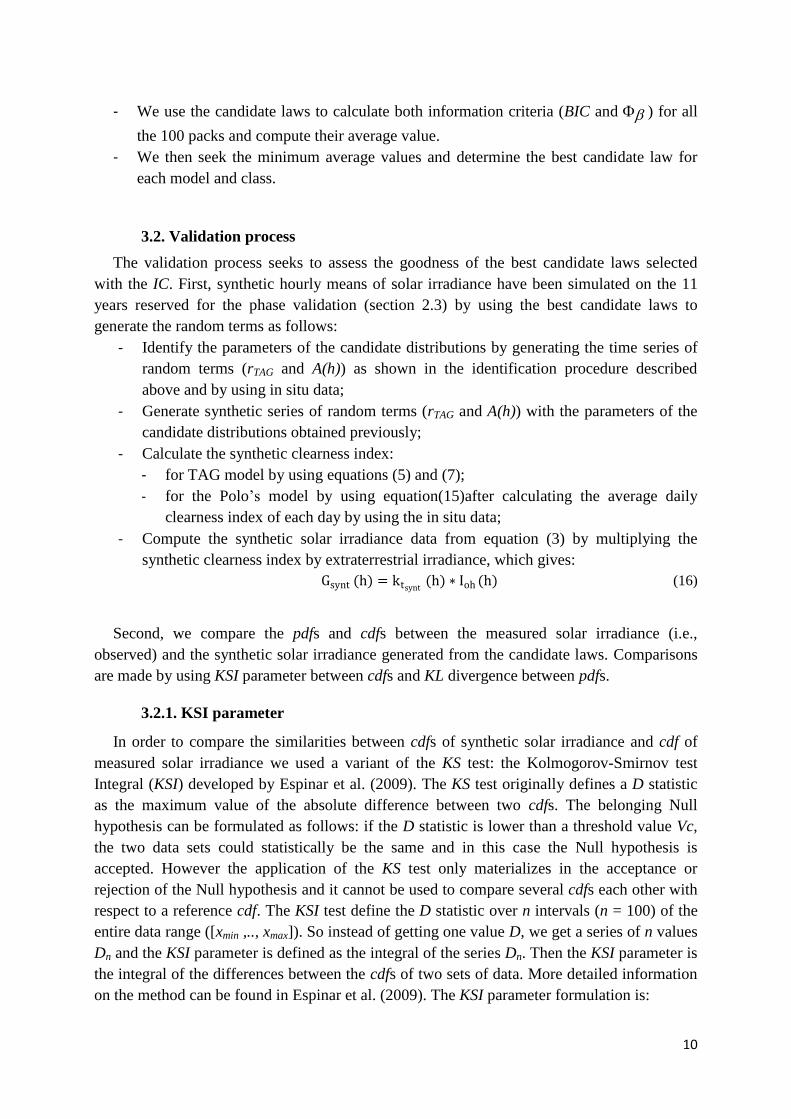
In case of the TAG model (Table 1), results are consistent concerning both IC. We find the
traditionally admitted Gaussian distribution law in the top three, but in the second position.
The most adequate law, in the sense of our selection criteria, is the logistic law, and the least
adequate is the extreme value law.
Table 1: Average values of criteria for all three candidate laws, regarding the TAG model.
Gaussian Logistic Extreme
value
12
BIC 35985 28045 44771
min 35973 28033 44759
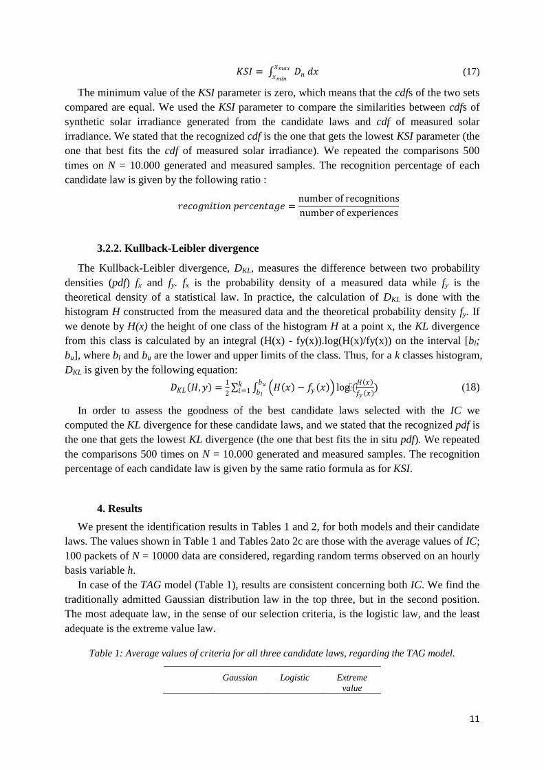
In the case of Polo's model (Tables 2a to 2c), after the IC test, we selected only the laws in
the top five best recognition rates. The negative values of the IC criteria in Table 2 are
justified by the impulsive nature (at maximum amplitude >> 1) of candidate laws. The BIC or
min criteria selected the same top five laws, regardless of the cloudiness class. These are the
Nakagami, Weibull, Beta, Gamma, and exponential laws. We ignore the other four laws in all
three tables. We note that for both models, the BIC and min criteria provide the same
ranking, which is normal because of the high quantity of considered data (N = 10000),
remember that both criteria are consistent (almost certain convergence). Neither criteria offers
better benefit than the other. In Tables 2a to 2c, the results are quite different for the different
classes of cloudiness; and this is justified by the variability of the model according to the
intensity of solar irradiance. Regarding the C1 and C2classes, the beta and Nakagami laws are
clearly distinguishable from the Weibull law, whereas the latter differs a little from the
gamma law (in the top two) but differs strongly from the other three candidates in the case of
low cloudiness (class C3).
Table 2: Average values of criteria for the laws in the top five, according to the three classes
of cloudiness for Polo's model.
(a) class C1
Beta Weibull Exponential Gamma Nakagami
BIC -14 897 -14 748 -14 130 -14 572 -14 938
min -14 915 -14 767 -14 139 -14 570 -14 957
(b) class C2
Beta Weibull Exponential Gamma Nakagami
BIC -9 965 -9 664 -8 527 -9 335 -9 944
min -9 983 -9 682 -8 537 -9 354 -9 962
(c) class C3
Beta Weibull Exponential Gamma Nakagami
BIC -11202 -11577 -10883 -11507 -11285
min -11220 -11596 -10893 -11526 -11595
13
5. Validation of models
To discuss the previous findings, the validation method described above has been used to
assess the goodness of the best candidate laws. In view of the IC values obtained at the stage
when laws are selected, we apply the validation method on all the five candidate laws and
present only the more significant results, those of the laws adopted in the top two. In Tables 3
and 4, we present, regarding the TAG model and then Polo's model, the recognition
percentages of each of the top two laws following the considered KL distance and KSI
parameter.
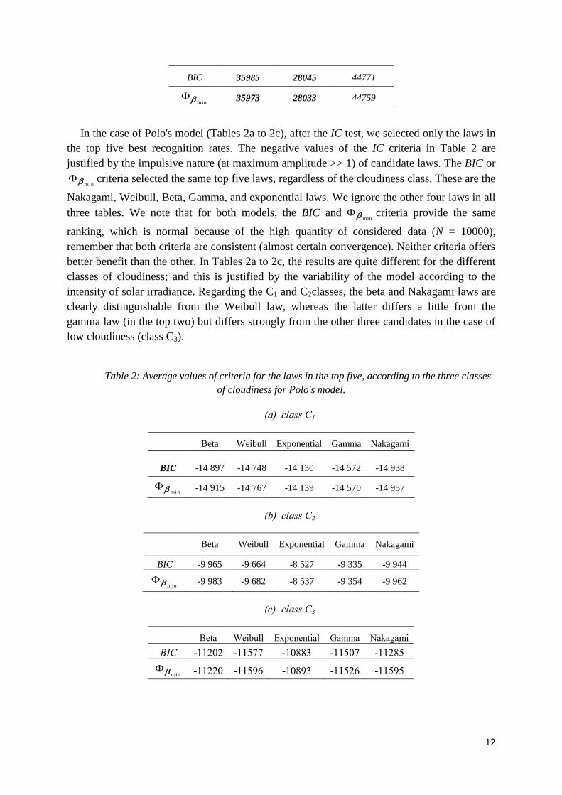
In the case of the TAG model, results in Table 3 confirm the findings of Table 1. These
results show that the IC-based method permits to identify the probabilistic distributions
introduced in the TAG model. We can therefore accept that a white logistical random term
yields to a best representation of the error associated with the model proposed by Aguiar and
Collares-Pereira (1992) rather than a Gaussian one, which would confirm Polo's findings
(2011). This method also contributes to the highlighting of the time invariance of distribution
laws representing the random term.
Table 3: Recognition percentage according to the KSI parameter and KL distances between measured
and generated laws for the TAG model.
Gaussian Logistic
KSI 35% 65%
KL 34% 66%
Table 4: Recognition percentage according to the KSI parameter and KL distances between
measured and generated laws for Polo's model.
class C1 class C2 class C3
Beta Nakagami Beta Nakagami Gamma Weibull
KSI 33% 67% 37,2% 68,2% 48% 52%
KL 33,2% 66,8% 38,2% 61,8% 41,2% 59,8%
Results in Table 4 confirm that the IC-based method allows the identification of the
probabilistic distributions introduced by the Polo's model in case of low (C3) or high
cloudiness (C1). In the case of partial cloudiness (C2), the validation process recognizes the
Nakagami law as being the distribution law of measured data, whereas the proximity of the IC
values does not permit us to definitively decide between Nakagami and Beta in the
identification process. In Figure 1, we provide the pdf (a) and the cdf (b) of five candidate
laws in the event of the Polo’s model to the disputed case of class C2 for 10000 values. We
see the similarity of the curves, and their behavior is close to the measured values for the Beta
and Nakagami laws, and thus it is difficult to decide definitively between these two laws in
case of partial cloudiness. Despite this difficulty, the results are converging since the IC-based
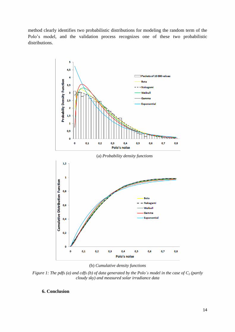
14
method clearly identifies two probabilistic distributions for modeling the random term of the
Polo’s model, and the validation process recognizes one of these two probabilistic
distributions.
(a) Probability density functions
(b) Cumulative density functions
Figure 1: The pdfs (a) and cdfs (b) of data generated by the Polo’s model in the case of C2 (partly
cloudy sky) and measured solar irradiance data
6. Conclusion
15
In this article, we have tried to improve modeling of the distributions involved in generation
models of synthetic solar irradiance in the inter-tropical zone.
We analyzed 14 years of solar ground irradiance measurements from two weather stations
located in French Guiana with a method based on IC. This method has permitted the
identification of the probability laws that best describe the statistical distribution of each
random term playing in two generation models of synthetic solar irradiance: Aguiar and
Pereira's TAG model and Polo's model.
The identified probability laws were validated by comparing the synthetic data generated
over 11 different years with in situ measured data and by using the KL divergence and KSI
parameter as comparison criteria. A strong correlation was noted in Aguiar and Pereira's TAG
model between the identified and validated probabilistic laws. This result demonstrates the
non-Gaussian nature of the random term of the original autoregressive model (1). Polo’s
model also found good matches between these two probability laws in cases of low and high
cloudiness.
In the case of partial cloudiness, the proximity of the values of identification criteria does
not permit us to definitively decide between these two laws, whereas the validation process
recognizes the Nakagami law as being the distribution law of measured data.
In conclusion, a new IC-based method has been defined and implemented on two models
with results that ensure the identification of the probability laws that best describe the
statistical distribution of the random terms of the two models. This method permits the
modeling of synthetic solar irradiance data comparable in their statistical content to the
measured solar irradiance data. This method could be extended to other measurement sites
and applied to other synthetic generation models of hourly or daily solar data to validate these
conclusions on a larger scale.
Acknowledgments
The authors thank the FEDER European program in French Guiana and Meteo France, who
enabled the realization of this study within the SOLAREST research project.
16
Appendix
We recall here the probability distribution of the various candidate laws used in this paper.
1. For the TAG model, three laws are considered:
• The Gaussian law
With µ being the average of the distribution and σ the standard deviation of distribution.
The extreme value law
Rxeexf
xx
e
,),,(
)()(
1
withµ and σ being the parameters of the form of the distribution.
The logistic law
Rxe
es
sxf s
x
s
x
,
1
1),,(
)(
2
With µ being the mean and s a parameter of the form linked to the variance.
2. For the Polo-based model, nine laws are considered:
The Beta law
]1,0[
)1(
)1(),,(
1
0
11
11
x
dyyy
xxxf
= 0 otherwise
with both and being the form and distribution parameters.
The Gamma law
0)(
1),,( 1
xexxf x
= 0 otherwise
With being a parameter of form and distribution, an intensity parameter, and Г() the gamma
function.
The exponential law
Rxexfx
,
2
1),,(
22
2)(
17
0,1
),(
xexf
x
= 0 otherwise
With µ being the mean and the distribution.
The Nakagami law
0,)(
12),,(
212
xexm
mmxf
xmm
m
= 0 otherwise,
With m being a form parameter, a parameter permitting to control the propagation of the distribution,
and (m) the gamma function.
The Rayleigh law
0x
= 0 otherwise,
With m being the distribution mode.
The Rice law
0,),,(
22
22
220
xe
xxsIsxf
sxm
= 0 otherwise,
With s and σ being the form and distribution parameters, andI0 being the Bessel function of the 1st kind
of the 0th order.
The Weibull law with two parameters
0,),,(
1
xexk
sxf
kxk
= 0 otherwise,
With k being a form parameter and a scale parameter.
The inverse Gaussian law
0,2
),,(2
2
2
)(
3
xex
xf x
x
= 0 otherwise,
With µ being the mean and a form parameter.
22
2
2),( m
x
em
xmxf
18
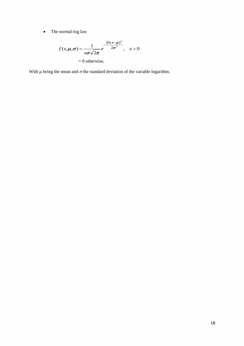
The normal-log law
0,2
1),,(
2
2
2
)(ln
xex
xf
x
= 0 otherwise,
With µ being the mean and the standard deviation of the variable logarithm.
19
List of abbreviation
Clearness index definition
kt : clearness index
Ioh : global irradiance on a horizontal plane
Isc : irradiance produced by the solar constant
E0 : correction factor of eccentricity
z : solar zenithal angle
TAG model
kt(h) : clearness index of the TAG model
y(h) : normalized clearness index of the TAG model
rTAG(h) : random term of the TAG model
KT) : correlation coefficient depending on the KT index
h : hourly variable time
KT : monthly average of the daily clearness index
ktm(KT,h) : hourly average of kt(h)
(KT, h) : standard deviation of kt(h)
Polo model
kt(h) : synthetic clearness index of the Polo model at a time h
ktm(j) : average daily value of the clearness index for day j
A(h) : random amplitude of the fluctuation of the clearness index for the hour h
sign(s) : sign of the random signal
s : realization of a normal Gaussian distribution centered with zero mean and standard
deviation unit
h : time
20
References
Aguiar, R.J., Collares-Pereira, M., Conde, J.P., 1988. Simple procedure for generating sequences of
daily radiation values using a library of Markov transition matrices. Solar Energy. 40(3), 269-279.
Aguiar, R., Collares-Pereira, M., 1992. TAG: A time-dependent, autoregressive, Gaussian model for
generating synthetic hourly radiation. Solar Energy. 49(3), 167-174.
Akaike, H., 1974. A new look at the statistical model identification. IEEE Trans. on Automatic
Control. 19(6),716-723.
AlataO., Olivier C., Pousset Y.,2013. Law recognitions by information criteria for the statistical
modeling of small scale fading of the radio mobile channel. Signal Processing. 93(5), 1064-1078.
Amado, M., Poggi, F., 2012. Towards solar urban planning: A new step for better energy performance.
Energy Procedia. 30, 1261-1273.
Bilbao, J., Miguel, A., Franco J.A., Ayuso, A., 2004. Test reference year generation and evaluation
methods in the continental Mediterranean area. Journal of Applied Meteorology. 43, 390-400.
Boland, J.,1995..Time-series analysis of climatic variables. Solar Energy. 55(5), 377-388.
Boland. J., 2008. Time series modelling of solar radiation, in: Badescu, V.(Ed.),Modeling Solar
Radiation at the Earth’s Surface: Recent Advances. Springer-Verlag, Berlin, pp. 283-312.
El Matouat, A., Hallin, M., 1996. Order selection, stochastic complexity and Kullback–Leibler
information, in Athens Conference on Applied Probability and Time Series Analysis: Volume II: Time
Series Analysis In Memory of E.J. Hannan. Springer-Verlag, Berlin, pp 291-299.
Espinar, B., Ramirez, L., Drews, A., Beyer, H.G., Zarzalejo, L.F., Polo, J., Martin, L., 2009. Analysis
of different comparison parameters applied to solar radiation data from satellite and German
radiometric stations. Solar Energy. 83, 118–125.
Graham, V.A., Hollands, K.G.T., Unny, T.E., 1988. A time series model for Kt with application to
global synthetic weather generation. Solar Energy. 40(2), 83-92.
Hannan, E.J., Quinn, B.G., 1979. The determination of the order of an autoregression. . Journal of the
Royal Statistical Society. 41(2), 190-195.
Hansen, C.W., Stein, J.S., Ellis, A., 2010. Statistical criteria for characterizing irradiance time series.
Sandia Report, SAND2010-7314.
Jouzel, F., Olivier, C., El Matouat, A., 1998. Information criteria based edge detection, in: Theodoridis,
S. (Ed.), Signal Processing IX: Proceedings of EUSIPCO-98, Ninth European Signal Processing
Conference, Rhodes (Greece), 8-11 September 1998.Typorama Editions, pp. 997-1000.
Larrañeta, M., Moreno-Tejera, S., Silva-Pérez, M.A., Lillo-Bravo, I. 2015. An improved model
for the synthetic generation of high temporal resolution direct normal irradiation time series. Solar
Energy. 122, 517-528
Linares-Rodríguez, A., Antonio Ruiz-Arias, J.,Pozo-Vázquez, D.J., Tovar-Pescador.,2011. Generation
of synthetic daily global solar radiation data based on ERA-Interim reanalysis and artificial neural
networks. Energy. 36(8), 5356-5365.
Marie-Joseph, I., Linguet, L., Gobinddass, M.L., Wald, L., 2013. On the applicability of the Heliosat-2
method to assess surface solar irradiance in the Intertropical Convergence Zone, French Guyana.
International Journal of .Remote Sensing. 34(8), 3012-3027.
Mellit, A., Kalogirou, S.A., Shaari, S., Salhi, H., Hadj Arab, A., 2008. Methodology for predicting
sequences of mean monthly clearness index and daily solar radiation data in remote areas: Application
for sizing a stand-alone PV system. Renewable Energy. 33(7), 1570-1590.
21
Muselli, M., Poggi, P., Notton, G., Louche, A., 1998. Improved procedure for stand-alone photovoltaic
systems sizing using METEOSTAT satellite images. Solar Energy. 62, 429-444.
Olivier, C., Alata, O., 2009. The information criteria: Examples of applications in image and signal
processing, in Optimization in Image and Signal Processing. P. Siarry ed., ITSE Ltd., London and
John Wiley& Sons, Inc., NJ, pp. 79-110.
Poggi, P., Notton, G., Muselli, M., Louche, A., 2000. Stochastic study of hourly total solar radiation in
Corsica using a Markov model. International Journal of Climatology 20, 1843–1860.
Polo, J., Zarzalejo, L.F., Marchante, R., Navarro, A.A., 2011. A simple approach to the synthetic
generation of solar irradiance time series with high temporal resolution. Solar Energy. 85, 1164-1170.
Rissanen, J., 1989. Stochastic Complexity in Statistical Inquiry. World Scientific, New Jersey.
Schwarz, G., 1978. Estimating the dimension of a model. Annals of Statistics. 6, 461-464.
Stanhill, G., Cohen, S., 2001. Global dimming: A review of the evidence for a widespread and
significant reduction in global radiation with discussion of its probable causes and possible
agricultural consequences. Agricultural and Forest Meteorology. 107(4), 255-278.
Tiba, C., Fraidenraich, N., 2004. Analysis of monthly time series of solar radiation and sunshine hours
in tropical climates. Renewable Energy. 29(7),1147-1160.
WMO, 2008. Guide to Meteorological Instruments and Methods of Observation, seventh ed., World
Meteorological Organization, Switzerland.
Recommended