WP/15/22

Identifying Constraints to Financial Inclusion and Their Impact on GDP and Inequality:

A Structural Framework for Policy

Era Dabla-Norris, Yan Ji, Robert Townsend, and D. Filiz Unsal

© 2015 International Monetary Fund WP/15/22

IMF Working Paper

Strategy, Policy, and Review Department

Identifying Constraints to Financial Inclusion and Their Impact on GDP and Inequality:

A Structural Framework for Policy1

Prepared by Era Dabla-Norris, Yan Ji, Robert Townsend, and D. Filiz Unsal

Authorized for distribution by David Marston

January 2015

Abstract

We develop a micro-founded general equilibrium model with heterogeneous agents to identify pertinent constraints to financial inclusion. We evaluate quantitatively the policy impacts of relaxing each of these constraints separately, and in combination, on GDP and inequality. We focus on three dimensions of financial inclusion: access (determined by the size of participation costs), depth (determined by the size of collateral constraints resulting from limited commitment), and intermediation efficiency (determined by the size of interest rate spreads and default possibilities due to costly monitoring). We take the model to a firm-level data from the World Bank Enterprise Survey for six countries at varying degrees of economic development—three low-income countries (Uganda, Kenya, Mozambique), and three emerging market countries (Malaysia, the Philippines, and Egypt). The results suggest that alleviating different financial frictions have a differential impact across countries, with country-specific characteristics playing a central role in determining the linkages and trade-offs between inclusion, GDP, inequality, and the distribution of gains and losses.

JEL Classification Numbers: E23, E44, E69, O11, O16, O57.

Keywords: Financial inclusion, inequality, income distribution, hetergenous agents.

Author’s E-Mail Address: edablanorris@imf.org, jiy@mit.edu, rtownsend@mit.edu, dunsal@imf.org _____________________ 1 This paper is part of a research project on macroeconomic policy in low-income countries supported by U.K.'s Department for International Development (DFID). This paper should not be reported as representing the views of DFID. We thank A. Banerjee, A. Auclert, A. Berg, F. Buera, S. Claessens, W. W. Dou, D. Marston, C. Pattillo, R. Portillo, A. Simsek, I. Werning, H. Zhang, and participants in the IMF Workshop on Macroeconomic Policy and Inequality and the MIT Macro and Development Seminar for helpful comments.

This Working Paper should not be reported as representing the views of the IMF. The views expressed in this Working Paper are those of the author(s) and do not necessarily represent those of the IMF or IMF policy. Working Papers describe research in progress by the author(s) and are published to elicit comments and to further debate.

Contents Page

1. Introduction…………………………………………………………………..…….. 42. Literature Review ………………………………………………………….............. 83. The Model ………………………………………………………………….……… 103.1 Individuals ……………………………………………………………………........ 11 3.1.1 Savings Regime……………………………………………………………….. 13 3.1.2 Credit Regime ……………………………………………………………....... 14 3.1.3 Occupational Choice …………………………………. ………………….... 21 3.2 Competitive Equilibrium ………………………………………………................ 23 4. Data and Calibration ……………………………………………………………… 245. Evaluation of Policy Options ……………………………………………………… 285.1 Reducing the Participation Cost……………………………………………………. 30 5.2 Relaxing Collateral Constraints ……………………………………………………. 31 5.3 Increasing Intermediation Efficiency ……………………………………………... 34 5.4 Interactions Among Three Financial Parameters ………………………………… 35 5.5 Impact on GDP and Inequality: A Numerical Comparison ……………………… 38 5.6 Welfare Analysis ………………………………………………………………… 40 6. Conclusion ………………………………………………………………………… 43

TABLES 1. Overview of the Data ……………………………………………………………. 252. Data, Model and Calibrated Parameters ………………………………………… 263. The Impact of Financial Deepening of Various Forms of GDP per Capita,

TFP and Income Inequality ………………………………………………………. 394. The Impact of Financial Deepening of Various Forms of GDP per Capita,

TFP and Income Inequality ………………………………………………………. 40FIGURES

1. Lending Interest Rate, Monitoring Frequency, Cost of Capital,and Leverage Ratio ……………………………………………………………… 21

2. The Occupation Choice Map in the Two Regimes ……………………………… 223. Comparative Statics: Credit Participation Cost–Low-Income Countries ………. 314. Comparative Statics: Credit Participation Cost–Emerging Market Countries …… 325. Comparative Statics: Collateral Constraint–Low-Income Countries …………… 346. Comparative Statics: Collateral Constraint–Emerging Market Countries ………. 357. Comparative Statics: Intermediation Cost–Low-Income Countries ……………. 368. Comparative Statics: Intermediation Cost–Emerging Market Countries ………. 379. The Increase in Relative GDP per Capita When the Borrowing Constraint is

Relaxed by 20% for Different Financial Participation Costs and Intermediation Costs ……………………………………………………. 38

10. The Impact of Financial Deepening on Welfare Redistribution ………………… 41REFERENCES………………………………………………………………………….. 45

1 Introduction

Financial deepening has accelerated in emerging market and low-income countries over the past

two decades. The record on financial inclusion, however, has not kept apace. Large amounts of

credit do not always correspond to broad use of financial services, as credit is often concentrated

among the largest firms. Moreover, firms in developing countries evidently continue to face barriers

in accessing financial services. For instance, 51 percent of firms in advanced economies use a bank

loan or line of credit as compared with 34 percent in developing economies (World Bank, 2014).

Firms also differ in terms of their own identification of access to finance as a major obstacle to their

operations and growth: firms in developing countries identify limited availability and high cost of

financing as a major problem.1

These considerations warrant a tractable framework that allows for a systematic examination of

the linkages between financial inclusion, GDP, and inequality. Moreover, there is a need for better

understanding of the economic channels through which these relationships are sustained. Given

that financial inclusion is multi-dimensional, involving both participation barriers and financial

frictions that constrain credit availability, policy implications to foster financial inclusion are likely

to vary across countries. In this paper, we develop a micro-founded general equilibrium model to

address these issues. This approach offers a consistent framework to elucidate the linkages between

financial inclusion, GDP, and inequality, and to quantify the impact of specific policy changes. This

can help guide policy makers in prioritizing between different financial sector policies depending

upon their goals.

In the model, agents are heterogeneous – distinguished from each other by wealth and talent.

Individuals choose in each period whether to become an entrepreneur or to supply labor for a wage.

Workers supply labor to entrepreneurs and are paid the equilibrium wage. Entrepreneurs have

access to a technology that uses capital and labor for production. In equilibrium, only talented

individuals with a certain level of wealth choose to become entrepreneurs. Untalented individuals,

1This problem is more acute for smaller firms and for those in the informal sector. For instance, in developingeconomies, 35 percent of small firms report that access to finance is a major obstacle to their operations, comparedwith 25 percent of large firms in developing economies and 8 percent of large firms in advanced economies (WorldBank, 2014). In this paper, we focus primarily on formal sector firms.

4

or those who are talented but wealth-constrained, are unable to start a profitable business, choosing

instead to become wage earners. Thus, occupational choices determine how individuals can save

and also what risks they can bear, with long-run implications for growth and the distribution of

income.

The model features an economy with two “financial regimes”, one with credit and one with

savings only. Individuals in the savings regime can save (i.e., make a deposit in financial institutions

to transfer wealth over time) but cannot borrow. Participation in the savings regime is free, but

individuals must may a participation cost to borrow. The size of this participation cost is one of

the determinants of financial inclusion, capturing the fixed transactions costs and high annual fees,

documentation requirements, and other access barriers facing firms in developing countries.

Once in the credit regime, individuals can obtain credit, but its size is constrained by two

additional types of financial frictions – limited commitment and asymmetric information. These

distort the allocation of capital and entrepreneurial talent in the economy, lowering aggregate

total factor productivity (TFP). The first financial friction is modeled in the form of endogenous

collateral constraints, which arise from the imperfect enforceability of contracts. Entrepreneurs have

to post collateral in order to borrow. The amount/value of collateral is thus another determinant

of financial inclusion, affecting the amount of the credit available. The second financial friction

arises from asymmetric information between banks and borrowers. In this environment, interest

rates charged on borrowing must cover the cost of monitoring of highly-leveraged firms. Because

more productive and poorer agents are more likely to be highly leveraged, the ensuing higher

intermediation cost is another source of inefficiency and financial exclusion. As only highly leveraged

firm are monitored, firms face differential costs of capital and may chose not to borrow even when

credit is available.

In our model, greater financial inclusion impacts GDP and inequality primarily through two

channels. First, it allows for a more efficient allocation of funds among entrepreneurs, thereby

increasing aggregate output. This occurs as funds are channeled to talented entrepreneurs, increasing

their output disproportionately more than that of less-talented ones. Second, more efficient financial

contracts limit waste from financial frictions (e.g., the credit participation and monitoring costs)

5

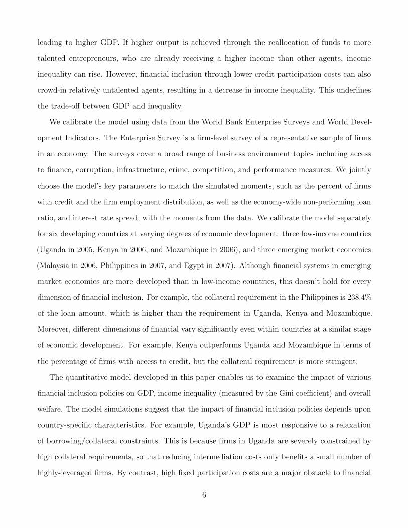
leading to higher GDP. If higher output is achieved through the reallocation of funds to more

talented entrepreneurs, who are already receiving a higher income than other agents, income

inequality can rise. However, financial inclusion through lower credit participation costs can also

crowd-in relatively untalented agents, resulting in a decrease in income inequality. This underlines

the trade-off between GDP and inequality.

We calibrate the model using data from the World Bank Enterprise Surveys and World Devel-

opment Indicators. The Enterprise Survey is a firm-level survey of a representative sample of firms

in an economy. The surveys cover a broad range of business environment topics including access

to finance, corruption, infrastructure, crime, competition, and performance measures. We jointly

choose the model’s key parameters to match the simulated moments, such as the percent of firms

with credit and the firm employment distribution, as well as the economy-wide non-performing loan

ratio, and interest rate spread, with the moments from the data. We calibrate the model separately

for six developing countries at varying degrees of economic development: three low-income countries

(Uganda in 2005, Kenya in 2006, and Mozambique in 2006), and three emerging market economies

(Malaysia in 2006, Philippines in 2007, and Egypt in 2007). Although financial systems in emerging

market economies are more developed than in low-income countries, this doesn’t hold for every

dimension of financial inclusion. For example, the collateral requirement in the Philippines is 238.4%

of the loan amount, which is higher than the requirement in Uganda, Kenya and Mozambique.

Moreover, different dimensions of financial vary significantly even within countries at a similar stage

of economic development. For example, Kenya outperforms Uganda and Mozambique in terms of

the percentage of firms with access to credit, but the collateral requirement is more stringent.

The quantitative model developed in this paper enables us to examine the impact of various

financial inclusion policies on GDP, income inequality (measured by the Gini coefficient) and overall

welfare. The model simulations suggest that the impact of financial inclusion policies depends upon

country-specific characteristics. For example, Uganda’s GDP is most responsive to a relaxation

of borrowing/collateral constraints. This is because firms in Uganda are severely constrained by

high collateral requirements, so that reducing intermediation costs only benefits a small number of

highly-leveraged firms. By contrast, high fixed participation costs are a major obstacle to financial

6

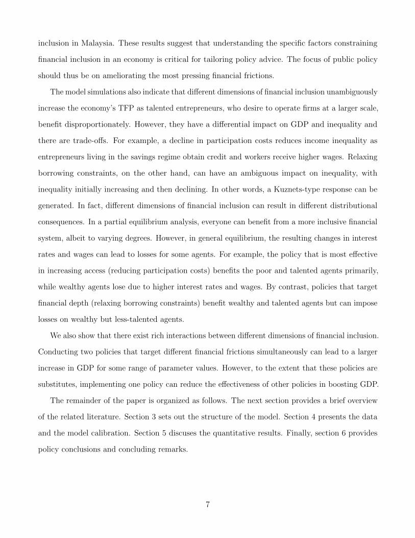
inclusion in Malaysia. These results suggest that understanding the specific factors constraining

financial inclusion in an economy is critical for tailoring policy advice. The focus of public policy

should thus be on ameliorating the most pressing financial frictions.

The model simulations also indicate that different dimensions of financial inclusion unambiguously

increase the economy’s TFP as talented entrepreneurs, who desire to operate firms at a larger scale,

benefit disproportionately. However, they have a differential impact on GDP and inequality and

there are trade-offs. For example, a decline in participation costs reduces income inequality as

entrepreneurs living in the savings regime obtain credit and workers receive higher wages. Relaxing

borrowing constraints, on the other hand, can have an ambiguous impact on inequality, with

inequality initially increasing and then declining. In other words, a Kuznets-type response can be

generated. In fact, different dimensions of financial inclusion can result in different distributional

consequences. In a partial equilibrium analysis, everyone can benefit from a more inclusive financial

system, albeit to varying degrees. However, in general equilibrium, the resulting changes in interest

rates and wages can lead to losses for some agents. For example, the policy that is most effective

in increasing access (reducing participation costs) benefits the poor and talented agents primarily,

while wealthy agents lose due to higher interest rates and wages. By contrast, policies that target

financial depth (relaxing borrowing constraints) benefit wealthy and talented agents but can impose

losses on wealthy but less-talented agents.

We also show that there exist rich interactions between different dimensions of financial inclusion.

Conducting two policies that target different financial frictions simultaneously can lead to a larger

increase in GDP for some range of parameter values. However, to the extent that these policies are

substitutes, implementing one policy can reduce the effectiveness of other policies in boosting GDP.

The remainder of the paper is organized as follows. The next section provides a brief overview

of the related literature. Section 3 sets out the structure of the model. Section 4 presents the data

and the model calibration. Section 5 discuses the quantitative results. Finally, section 6 provides

policy conclusions and concluding remarks.

7

2 Literature Review

A growing theoretical literature has emphasized the aggregate and distributional impacts of financial

intermediation in models of occupational choice and financial frictions. This theoretical framework

was first introduced by Banerjee and Newman (1993) to capture the process of economic development.

Lloyd-Ellis and Bernhardt (2000) extended the model to explain income inequality and the existence

of a Kuznets curve. Cagetti and Nardi (2006) build on the framework to show that the introduction

of a bequest motive generates lifetime savings profiles more consistent with data. In these studies,

improved financial intermediation leads to greater entry into entrepreneurship, higher productivity

and investment, and a general equilibrium effect that increases wages. Moreover, the models suggest

that the distribution of wealth or the joint distribution of wealth and productivity are critical.

A related literature has found sizeable impacts of improved financial intermediation on aggregate

productivity and income (Gine and Townsend, 2004; Jeong and Townsend, 2007, 2008; Amaral

and Quintin, 2010; Buera et al., 2011; Greenwood et al., 2013). Buera et al. (2011) incorporate

forward-looking agents in an occupational choice framework, showing that financial frictions account

for a substantial part of the observed cross-country differences in output per worker and aggregate

TFP. Moreover, Buera et al. (2012) focus on the general equilibrium effects of micro finance. They

find that the impact of scaling-up microfinance on per-capita income is small, because of the ensuing

redistribution of income from high-savers to low-savers, but the vast majority of the population

benefits from higher wages. Moll (2014) shows that the impact of financial frictions on GDP and

TFP depends on the persistence of idiosyncratic shocks, and that the short-run effects of financial

frictions tend to be larger than their long-run impacts.

Our model builds on this occupational choice framework, but with novel features. We focus on

several dimensions of financial inclusion within an economy. Although these dimensions have typically

been considered separately in the previous literature, our paper provides a unified framework for

examining them individually as well as jointly. Our model features three types of financial frictions:

fixed costs of credit entry, limited commitment, and asymmetric information. Unlike previous studies,

our model allows us to also uncover how different frictions interact with each other. Therefore, our

8

paper is related to studies in which multiple financial frictions co-exist and are compared. Clementi

and Hopenhayn (2006) and Albuquerque and Hopenhayn (2004) argue that moral hazard and

limited commitment have different implications for firm dynamics. Abraham and Pavoni (2005)

and Doepke and Townsend (2006) discuss how consumption allocations differ under moral hazard

with and without hidden savings versus full information. Martin and Taddei (2013) study the

implications of adverse selection on macroeconomic aggregates and contrast them with those under

limited commitment. Karaivanov and Townsend (2014) estimate the financial/information regime

in place for households (including those running businesses) in Thailand and find that a moral

hazard constrained financial regime fits the data best in urban areas, while a more limited savings

regime is more applicable for rural areas. Similarly, Paulson et al. (2006) argue that moral hazard

best fits the data in the more urban Central region of Thailand but not in the more rural Northeast.

Kinnan (2014) uses a different metric based on the first-order conditions characterizing optimal

insurance under moral hazard, limited commitment and hidden income to distinguish between

these regimes in Thai data. Finally, Moll et al. (2014) use a general equilibrium framework that

encompasses different types of frictions, and examines the equilibrium interactions between various

frictions. Our paper is related to these studies, but constitutes a normative policy analysis. By

developing a quantitative macroeconomic framework and disciplining it with micro data, we shed

light on a number of policy issues. For instance, what financial frictions are most relevant for

the economy’s GDP and income inequality? And what is the impact of alleviating these financial

frictions individually or jointly?

Our paper is also related to a large empirical literature on the real effects of credit. The view that

financial deepening spurs economic growth is supported by empirical evidence (King and Levine,

1993; Levine, 2005). Regression-based analyses at the aggregate level reveal a strong correlation

between broad measures of financial depth (such as M2 or credit to GDP) and economic growth.

For firms, access to finance is positively associated with innovation, job creation, and growth

(Beck et al., 2005; Ayyagari et al., 2008). There is also evidence that aggregate financial depth is

positively associated with poverty reduction and income inequality (Beck et al., 2007; Clarke et al.,

2006). Cross-sectional regression analysis, however, can be problematic as causality cannot easily be

9

established, causal mechanisms are difficult to pin down, and policy evaluation is more challenging.

Moreover, the implicit assumptions of stationarity and linearity in regression analysis could be

incorrect, even after taking logs and including lags, if these variables lie on complex transitional

growth paths (Townsend and Ueda, 2006). The advantage of using a structural framework such as

ours lies in capturing salient features of the economy and the pertinent financial sector frictions for

which rules of thumb, based on purely empirical evidence, fail to account for.

Our paper is also broadly related to the literature on misallocation (Hsieh and Klenow, 2009;

Caselli and Gennaioli, 2013; Midrigan and Xu, 2014; Moll, 2014) and inequality (Davies, 1982;

Huggett, 1996; Aghion and Bolton, 1997; Castaneda et al., 2003; Nardi, 2004). Our contribution is

to show that policy options that target different financial sector frictions have different impacts

on resource allocation and inequality. More importantly, even for the same policy, the impacts on

inequality can differ as these impacts are contingent on country-specific characteristics.

3 The Model

The economy is populated by a continuum of agents of measure one. Agents are heterogeneous in

terms of initial wealth b and talent z.

Each agent lives for two periods. In the first period, the agent makes credit participation,

occupational choice, and investment decisions, taking the optimal consumption/bequest decision

made in the second period as given. In the second period, the agent realizes income as wage or

business profit, depending on the occupation, and makes consumption and bequest decisions to

maximize utility. Each agent has an offspring, whose wealth is equal to the bequest, and talent is

drawn from a stochastic process.2 The time sub-script t is omitted unless necessary.

2The successor of an agent can be interpreted as the reincarnation of the original agent with potentially newtalent.

10

3.1 Individuals

The agent generates utility only in the second period through consumption and a bequest to her

offspring. The utility function is Cobb-Douglas, given by

u(c, b′) = c1−ωb′ω, (3.1)

where c is consumption, and b′ is bequest. The bequest motive transfers wealth across periods,

which endogenously determines the economy’s wealth distribution. The assumption that utility is

generated by bequest rather than the offspring’s utility simplifies the analysis and captures the idea

of a tradition for bequest-giving following Andreoni (1989). However, it is equivalent to a myopic

savings rate for the same agent.

In the second period, the agent maximizes (3.1) by choosing c and b′ subject to the budget

constraint c+ b′ = W , where W denotes the second period wealth, which depends on initial wealth

and realized first-period income.

The Cobb-Douglas form implies that the optimal bequest rate is ω.3 Hence, the utility function

u(c, b′) is a linear function of end-of-period wealth (W ), i.e., the agent is risk neutral. This

implies that maximizing expected utility is equivalent to maximizing expected second-period wealth.

Therefore, in the first period, the agent chooses financial participation, occupation and investment

to maximize expected income.

In the first period, agents need to make an occupational choice between being a worker or an

entrepreneur. Each worker supplies one unit of labor, and the income realized in the first period is

equal to the equilibrium wage, w. The entrepreneur invests capital and labor, and obtains income

through business profit.

Talent is drawn from a Pareto distribution µ(z) with a tail parameter θ. The offspring inherits

the talent of her parents (or former self) with probability γ, otherwise, a new talent is drawn from

µ(z).4

3The value of ω affects the amount of wealth transferred from the current period to the next period. Therefore,ceteris paribus a higher ω implies that the economy would have a higher level of wealth.

4The shock to talent is interpreted as changes in market conditions that affect the profitability of individual skills

11

The entrepreneur has access to a production technology, the productivity of which depends on

the agent’s talent. The production function is

f(k, l) = z(kαl1−α)1−ν (3.2)

where 1− ν is the Lucas span-of-control parameter, representing the share of output accruing to

the variable factors. Out of this, a fraction α goes to capital, and 1− α goes to labor. Production

exhibits diminishing returns to scale, with ν > 0. Firms make profits, and capital depreciates by δ

after use.

Production fails with probability p, in which case output is zero and the agent is able to recover

only a fraction η < 1 of installed capital, net of depreciation in the second period. To simplify the

calculation, we assume workers get paid only when production is successful. Therefore, each worker

earns a wage with probability 1− p.

All agents can make a deposit in a financial institution so as to transfer income and initial

wealth within period for consumption and bequest. However, following Greenwood and Jovanovic

(1990) and Townsend and Ueda (2006), agents need to pay a fixed credit participation cost, ψ, to

obtain a borrowing contract from financial institutions. We assume that an agent lives in a ”credit”

regime, if the agent pays the cost ψ and can borrow; that an agent lives in a ”savings” regime, if

the agent doesn’t pay ψ and can thereby only saves. This cost can be considered as a contractual

fee or a bargaining cost with financial institutions. Intuitively, since workers do not invest, they

never demand external credit. Entrepreneurs may want to borrow in order to expand their firm

scale and profits. In equilibrium, the fixed entry cost ψ is more likely to exclude poor entrepreneurs

from financial markets, because this amounts to a larger fraction of their initial wealth. The next

section illustrates the structure of the borrowing contract in detail.

Note that both the wage and deposit interest rate are potentially time-varying and determined

endogenously by the labor and capital market clearing conditions. Given the equilibrium wage rate

w, and deposit interest rate rd, an agent of type (b, z) makes credit participation and occupational

as in Buera et al. (2011).

12

choice decisions to maximize expected income.

We solve the problem in two steps: first, the agent chooses her occupation conditional on the

regime she is living in; second, the agent chooses the underlying regime by comparing the expected

income that can be obtained in each regime. The next section presents the occupational choice

problem in the savings and credit regimes, respectively.

3.1.1 Savings Regime

Individuals living in the savings regimes cannot borrow from financial institutions—they have to

finance the project exclusively using their own resources.

In the first period, the goal of the agent is to maximize expected income. Given a certain initial

wealth, maximizing expected income is equivalent to maximizing expected end-of-period wealth,

W . Let π(b, z) be the expected end-of-period wealth function for an entrepreneur of type (b, z).

Denoting variables with superscript S for the savings only regime, one can write:

W S =

(1 + rd)b+ (1− p)w for workers

πS(b, z) for entrepreneurs(3.3)

where workers are paid only if production is successful, with a probability (1− p).5 Since agents

are risk-neutral, they choose to be workers if (1 + rd)b + (1− p)w > πS(b, z), and entrepreneurs

otherwise. Therefore, end-of-period wealth for an agent can be simply written as W S = max(1 +

rd)b+ (1− p)w, πS(b, z).

The wealth function πS(b, z) for entrepreneurs is obtained from the following maximization

problem,

πS(b, z) = maxk,l(1− p)[z(kαl1−α)1−ν − wl − δk + k] + pη(1− δ)k + (1 + rd)(b− k) (3.4)

5To simplify the computation, we do not explicitly track which firms hire which workers in our numericalsimulation. All agents receive the full wage income w with probability p, and receive nothing with probability 1− p.Since agents are risk-neutral in our model, they only care about the expected wage income, which is (1− p)w, whenmaking occupational choice decisions.

13

subject to

k ≤ b (3.5)

With probability 1− p, production succeeds, and the entrepreneur gets revenue (z(kαl1−α)1−ν −

wl− δk) plus k working capital. With probability p, production fails, and the entrepreneur can only

get a fraction η of end-of-period depreciated working capital. The last term in the maximization

problem accounts for wealth that is not used in production. The constraint reflects the fact that

the entrepreneur needs to finance capital through her own initial wealth.6

3.1.2 Credit Regime

Individuals living in the credit regime have access to external credit by paying an up-front credit

participation cost ψ. As workers receive no benefit from obtaining external credit, they do not

demand capital. Therefore, we only consider the entrepreneur’s problem in the credit regime.

Since our focus is on the macroeconomic impact of financial inclusion, we assume that the

financial sector is perfectly competitive, driving profits from intermediation to zero. This assumption

can be easily relaxed by adding a profit margin for intermediation to capture noncompetitive banking

sectors in most developing countries. This serves to increase the borrowing interest rates facing

entrepreneurs, but the model’s qualitative predictions remain the same.

In order to borrow, agents need to sign a contract with a financial institution. A financial

contract is characterized by three variables, (Φ,∆,Ω), where Φ is the amount of borrowing, ∆ is

the value of collateral, and Ω is the face value of the contract. The face value, Ω, is the amount of

money that needs to be repaid by the borrower if there is no default, which is determined by the

bank’s zero profit condition. For simplicity, we assume that collateral is interest bearing, that is,

agents earn the deposit interest rate rd on the value of collateral.

Although the financial contract doesn’t specify the lending interest rate, we can define the

implied interest rate in the following way:

6Note that the diminishing returns to scale property implies that there exists an unconstrained level of capitalkS(z). Entrepreneurs never want to operate their firms at a scale larger than this

14

rl =Ω

Φ− 1 (3.6)

rl would be potentially different for different entrepreneurs, depending on the terms of the

contract.

Similarly, the leverage ratio (the amount of borrowing relative to the size of collateral) is defined

as,

λ =Φ

∆(3.7)

If production fails, the entrepreneur may not be able to repay the debt face value Ω. If this

happens, the entrepreneur defaults and the financial institution seizes the interest-bearing collateral,

(1 + rd)∆ and the recovered value of depreciated working capital, η(1− δ)k. In equilibrium, since

highly-leveraged entrepreneurs default in case of a production failure, they are charged with a

higher lending interest rate in the event of success (to compensate for losses in event of failure).

We consider two types of financial frictions in the financial sector: (i) limited commitment, and

(ii) asymmetric information. The former imposes a form of ”credit rationing” on entrepreneurs

since they have to post collateral in order to borrow. For some entrepreneurs, this constraint is

binding. The latter friction increases the borrowing rate for entrepreneurs with default possibilities.

Specifically, the constraints imply the following:

Limited commitment In order to borrow, an entrepreneur needs to post collateral in the

financial institution. Suppose an entrepreneur can borrow Φ if an amount of collateral ∆ is posted.

Suppose further that contract enforcement is imperfect, therefore, she can abscond with a fraction

of 1/λ of the rented capital. The only punishment is that she will lose her collateral ∆ and the

interest earning on it. In equilibrium, entrepreneurs do not abscond only if Φ/λ < ∆. Therefore, the

bank is only willing to lend λ∆ to the entrepreneur if ∆ units of collateral are posted.7 This single

parameter λ ≥ 1 parsimoniously captures the degree of financial friction resulting from limited

commitment. A special case of λ = 1 implies that entrepreneurs cannot borrow.

7See Banerjee and Newman (2003), Buera and Shin (2013), and Moll (2014) for a similar motivation of this typeof constraint.

15

Asymmetric information There is asymmetric information between entrepreneurs and banks

(i.e. whether the production of a particular entrepreneur fails or not is only known to the entrepreneur

herself). Due to limited liability, entrepreneurs have a default option when production fails. This

implies that they could pay less if a production failure is reported and not discovered by banks.

All agents are truth-telling. However, this comes at a cost. Banks have a monitoring technology

through which they get information on the success of production at a cost proportional to the scale

of the production (denoted by χ). If entrepreneurs are caught cheating, then banks can legally

enforce the full repayment of the loan’s face value. As banks make zero profits in equilibrium, the

monitoring cost is borne by entrepreneurs when the financial contract is designed.

The bank’s optimal verification strategy follows Townsend (1979), which occurs if and only if

entrepreneurs cannot repay the face value of the loan. This happens when the entrepreneur is highly

leveraged and also experiences a production failure.8 To be more specific, when production succeeds,

entrepreneurs can repay the face value of the loan.9 Therefore, there is no incentive for the bank to

monitor. However, if a production failure is reported, banks monitor only if the loan contract is

highly leveraged. This is because a low-leveraged loan contract implies that entrepreneurs are not

borrowing much from the bank. Therefore, the required repayment is small, and can be covered

by the value of interest-bearing collateral ((1 + rd)∆) plus the value of recovered working capital

(η(1− δ)k), even if production fails. In this case, entrepreneurs have no incentive to lie because

regardless of the production outcome, they can and have to repay the face value of the loan. For

the same reason, banks have no incentive to monitor.

On the other hand, if the loan contract is highly-leveraged10, and if production fails, the amount

of money that entrepreneurs can repay is not sufficient to cover the face value of the loan. As a

8Implicitly assumed here is that entrepreneurs would not decline the repayment of the loan if they have sufficientfunds because the bank monitors and seizes the face value of the loan when default happens.

9This argument is trivial, since entrepreneurs would borrow to produce only if they can make profits. Therefore,when production succeeds the gross output should be at least higher than the capital input. On the other hand, ifthe entrepreneur defaults, the bank will monitor output and seize the face value of the loan. Thus, the entrepreneurhas no incentive to default.

10The threshold between low and high leverage ratio is derived by considering whether the value of interest-bearingcollateral plus the recovered working capital is sufficient to repay the face value of the loan. In particular, as wediscuss later, the loan contract is highly leveraged if η(1− δ)Φ + (1 + rd)∆ < Ω.

16

result, default happens. Finally, note that in this case entrepreneurs do have an incentive to lie

when production is successful because they know with high leverage they would repay less if a

production failure is reported. Therefore, to motivate truth-telling, banks verify all the results of

the highly-leveraged loan contract if a production failure is reported.

In the credit regime, the end-of-period wealth is denoted by

WC = πC(b, z)

where the superscript C refers to the credit regime. The agent chooses to pay the credit

participation cost when WC > W S.

We assume that banks cannot observe entreprenerus’ type (b, z), and therefore have to provide

a menu of contracts for entrepreneurs of different types (b, z). The entrepreneur of type (b, z)

chooses the optimal contract from the menu. Notice that the schedule of contracts is designed to be

incentive-compatible, namely, entrepreneurs of type (b, z) would have no incentive to imitate type

(b′, z′) and chooses the optimal contract of other entrepreneurs. Moreover, all loan contracts make

zero profits given that financial intermediation is perfectly competitive. Below, we first elaborate the

optimal contract for the entrepreneur of type (b, z). We then discuss why the contract is incentive

compatible.

To solve the optimal loan contract (Φ,∆,Ω) for the entrepreneur of type (b, z), we use the

following procedures:

First, notice that collateral is interest-bearing; therefore, entrepreneurs should be willing to

post all of their wealth net of credit participation cost, b− ψ as collateral instead of depositing a

fraction of it in a savings account. Hence, the collateral term, ∆ = b− ψ should belong to the set

of optimal loan contracts.11

Second, notice that entrepreneurs borrow to increase production scale and make higher profits.

Therefore, there is no reason to borrow more funds from the bank and not use them in production,

11Note that there might exist multiple optimal contracts for wealthy entrepreneurs, since they do not demandmuch credit. But all these contracts would result in an identical net outcome for both entrepreneurs and banks.The optimal contract we focus here is the one with the lowest leverage ratio, i.e., with all wealth b being posted ascollateral.

17

since this only increases the leverage ratio, which, in turn, potentially increases the cost of capital.

Hence, the amount of loan, Φ, should be equal to the amount of capital, k(b, z), if the loan contract

is optimal.

The above arguments suggest that the optimal loan contract chosen by the entrepreneur of type

(b, z) should be of the form (k(b, z), b− ψ,Ω), so Ω remains the only element to be determined.

The face value of the loan, Ω, in the optimal contract should be set by the bank such that the

bank makes zero profit knowing that only entrepreneurs of type (b, z) will choose it. From the bank’s

perspective, the expected payoff of this loan contract is (1−p)Ω+pmin(Ω, η(1−δ)k+(1+rd)(b−ψ)).

The first term refers to the payoff when production succeeds, which happens with probability (1−p).

In this case, the bank receives the full face value of the loan, Ω. The second term refers to the

payoff when production fails. When production fails, before repaying the debt, the entrepreneur’s

“net value” is equal to the recovered depreciated working capital, η(1− δ)k, plus the after-interest

value of collateral, (1 + rd)(b − ψ). The bank receives the full face value of the loan, Ω, if the

entrepreneur’s “net value” is sufficient to repay it. Otherwise, the bank only receives the ”net value”

due to limited liability, and the entrepreneur would end up with nothing. In sum, when production

fails, the bank receives either Ω or η(1− δ)k + (1 + rd)(b− ψ), whichever is smaller.

On the other hand, the cost of creating the loan contract, is equal to the after-interest value of loan,

(1 + rd)k, plus the expected cost of monitoring. Note that monitoring occurs only if entrepreneurs

cannot repay the loan, namely, when production fails and the net value, η(1− δ)k+ (1 + rd)(b−ψ),

is smaller the loan’s face value, Ω. In this case, a monitoring cost, χk, is incurred. Therefore,

the expected cost of monitoring is equal to the monitoring cost, χk, multiplied by the monitoring

rate. The monitoring rate is equal to the production failure rate, p, when entrepreneurs are

highly leveraged, i.e. η(1− δ)k + (1 + rd)(b− ψ) < Ω, and zero otherwise. The expected cost of

monitoring can be expressed as pχk · 1η(1−δ)k+(1+rd)(b−ψ)<Ω, where 1η(1−δ)k+(1+rd)(b−ψ)<Ω is an

indicator function, which equals to 1 if η(1− δ)k+ (1 + rd)(b−ψ) < Ω and 0 otherwise. Hence, the

cost of creating the loan contract is (1 + rd)k + pχk · 1η(1−δ)k+(1+rd)(b−ψ)<Ω.

The zero profit function is obtained when the expected payoff of the loan is equal to its cost,

18

(1− p)Ω + pmin(Ω, η(1− δ)k + (1 + rd)(b− ψ)) = (1 + rd)k + pχk · 1η(1−δ)k+(1+rd)(b−ψ)<Ω (3.8)

Equation (3.8) implies that in the optimal contract we consider, Ω is a function of k and b.

Thus Ω is pinned down by the zero profit condition, which is (3.8). The optimal contract chosen by

an entrepreneur of type (b, z) can be written as (k(b, z), b − ψ,Ω(k(b, z), b)), where k(b, z) is the

optimal amount of capital invested in production, and Ω(k(b, z), b) is determined by equation (3.8).

Therefore, to exactly characterize the optimal contract as a function of b and z, we only need to

know the optimal amount of capital, which is solved in the following problem.

The entrepreneur of type (b, z) chooses capital k and labor l optimally to maximize expected

production profit,

πC(b, z) = maxk,l(1− p)[z(kαl1−α)1−ν − wl + (1− δ)k − Ω + (1 + rd)(b− ψ)] (3.9)

+pmax(0, η(1− δ)k + (1 + rd)(b− ψ)− Ω)

subject to

k ≤ λ(b− ψ)

where, the term Ω in problem (3.9) is the solution to bank’s zero profit condition (3.8). The

solution to (3.8) and (3.9) determines the optimal capital investment k as a function of b and z,

and pins down the optimal contract.

In (3.9), the first term refers to the end-of-period wealth for the entrepreneur when production

succeeds. The second term refers to the case of production failure. The entrepreneur only has

something left if η(1− δ)k + (1 + rd)(b− ψ) > Ω, that is when the recovered depreciated working

capital plus the after-interest value of collateral is sufficient to repay the loan. Otherwise, the

entrepreneur will end up with zero wealth at the end of the period.

19

Finally, notice that all contracts offered by the bank are incentive-compatible, although talent

may not be observable. This implies that entrepreneurs of low talent have no incentive to pretend

to be highly-talented and ask for a different contract, or vice versa. To see this, divide both sides of

equation (3.8) by k,

(1− p)Ω

k+ pmin(

Ω

k, η(1− δ) + (1 + rd)

b− ψk

) = (1 + rd) + pχ · 1η(1−δ)+(1+rd) b−ψk<Ωk (3.11)

Equation (3.11) suggests that the implied gross lending interest rate, Ωk, only depends on the

inverse of the leverage ratio b−ψk

12, but not directly on the entrepreneur’s talent. That is, capital k

and talent z enter equation (3.11) only through the leverage ratio, which is observable. Therefore,

for all entrepreneurs, given the amount of capital they want to invest (or demand for credit) and

the amount of wealth they own (or collateral value), it is impossible to receive a lower interest

rate from the bank by cheating on talent. This result is obtained because it is assumed that the

recovered value of depreciated working capital doesn’t depend on entrepreneurs’ talent.

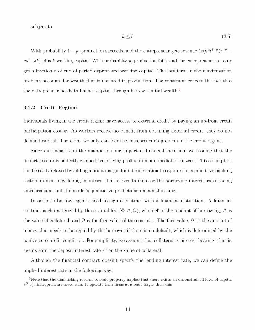
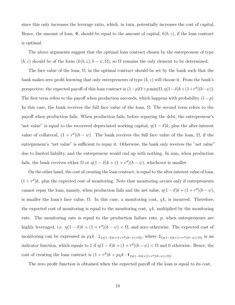
In Figure 1, we present how the lending interest rate, the probability of being monitored, and

the cost of monitoring change when entrepreneurs’ leverage ratio varies. As noted above, only

highly leveraged entrepreneurs are monitored. In particular, there is a threshold level of leverage

ratio (1.69), below which the probability of being monitored is zero, and thus both of the lending

interest rate and the cost of capital are equal to the deposit interest rate. If entrepreneurs increase

leverage beyond this threshold, they cannot repay the face value of the debt when production fails.

Therefore, the probability of being monitored is exactly equal to the production failure rate, p.

Since banks are making zero profits, the monitoring cost is completely borne by the entrepreneurs,

generating a higher cost of capital. Note that the cost of capital in this case is rd + pχ, which is

constant regardless of the leverage ratio. This is due to our assumption that the monitoring cost is

proportional to the scale of production but not the value of loan. Moreover, the implied lending

interest rate defined in equation (3.6) is strictly increasing in the leverage ratio when the leverage

12Note according to (3.7), the inverse of leverage ratio is defined as ∆Φ . In the optimal contract illustrated above,

∆ = b− ψ, and Φ = k.

20

Figure 1: Lending interest rate, monitoring frequency, cost of capital, and leverage ratio.

0 1 2 30

0.05

0.1

0.15

0.2

Leverage ratio

Lend

ing

inte

rest

rat

e

0 1 2 30

0.05

0.1

0.15

0.2

Leverage ratio

Pro

babi

lity

of b

eing

mor

nito

red

0 1 2 30

0.05

0.1

0.15

0.2

Leverage ratio

Cos

t of c

apita

l

The figure is plotted using rd = 0.05, η = 0.35, δ = 0.06, p = 0.15, χ = 0.3.

ratio is higher than its threshold. This is because banks have to be repaid more (as reflected by a

higher face value Ω) when production succeeds to compensate for larger losses when the project

fails due to higher leverage.

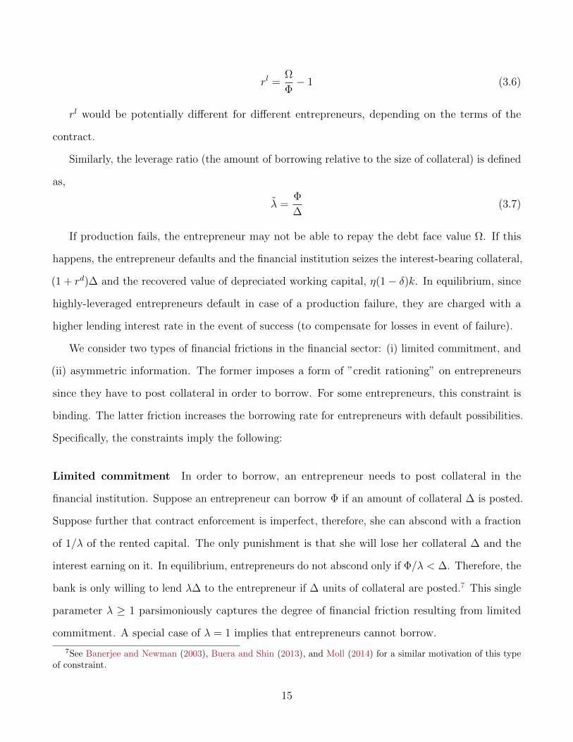
3.1.3 Occupational Choice

The occupation map is plotted according to the choice of occupation for agents with different talent

z and wealth b, and whether this choice is constrained by wealth. We identify four categories of

agents in the savings regime, separated by the solid lines in the left graph of Figure 2: unconstrained

workers, constrained workers, constrained entrepreneurs, and unconstrained entrepreneurs.

As shown in the figure, there is a certain threshold level of talent (1.3), below which an agent

always find that working for a wage is better than operating a firm. These people are identified as

unconstrained workers, suggesting that their talent is so low that they never find it is optimal to

become an entrepreneur. Above this talent level, the figure is further segmented into three regions.

In the left region, agents are talented, but do not have sufficient wealth, so they cannot operate

a firm at a profitable scale. Hence, they choose to be workers. These are constrained workers.

The middle region represents agents with sufficient wealth to operate a profitable firm but scale is

still constrained by wealth. These agents are constrained entrepreneurs. Agents belonged to the

right region of the figure choose to be entrepreneurs, operating a firm at the unconstrained scale,

with the marginal return of capital equal to the deposit interest rate. Thus, they are identified as

21

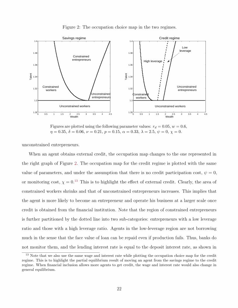
Figure 2: The occupation choice map in the two regimes.

0 0.5 1 1.5 2 2.5 3 3.5 4 4.51.28

1.3

1.32

1.34

1.36

1.38

1.4

Wealth

Tal

ent

Savings regime

0 0.5 1 1.5 2 2.5 3 3.5 4 4.51.28

1.3

1.32

1.34

1.36

1.38

1.4

Wealth

Tal

ent

Credit regime

High leverage

Low leverage

Unconstrained workers

Unconstrained entrepreneurs

Unconstrained workers

Constrained entrepreneurs

Constrained workers

Constrained workers

Unconstrained entrepreneurs

Figures are plotted using the following parameter values: rd = 0.05, w = 0.6,η = 0.35, δ = 0.06, ν = 0.21, p = 0.15, α = 0.33, λ = 2.5, ψ = 0, χ = 0.

unconstrained entrepreneurs.

When an agent obtains external credit, the occupation map changes to the one represented in

the right graph of Figure 2. The occupation map for the credit regime is plotted with the same

value of parameters, and under the assumption that there is no credit participation cost, ψ = 0,

or monitoring cost, χ = 0.13 This is to highlight the effect of external credit. Clearly, the area of

constrained workers shrinks and that of unconstrained entrepreneurs increases. This implies that

the agent is more likely to become an entrepreneur and operate his business at a larger scale once

credit is obtained from the financial institution. Note that the region of constrained entrepreneurs

is further partitioned by the dotted line into two sub-categories: entrepreneurs with a low leverage

ratio and those with a high leverage ratio. Agents in the low-leverage region are not borrowing

much in the sense that the face value of loan can be repaid even if production fails. Thus, banks do

not monitor them, and the lending interest rate is equal to the deposit interest rate, as shown in

13 Note that we also use the same wage and interest rate while plotting the occupation choice map for the creditregime. This is to highlight the partial equilibrium result of moving an agent from the savings regime to the creditregime. When financial inclusion allows more agents to get credit, the wage and interest rate would also change ingeneral equilibrium.

22

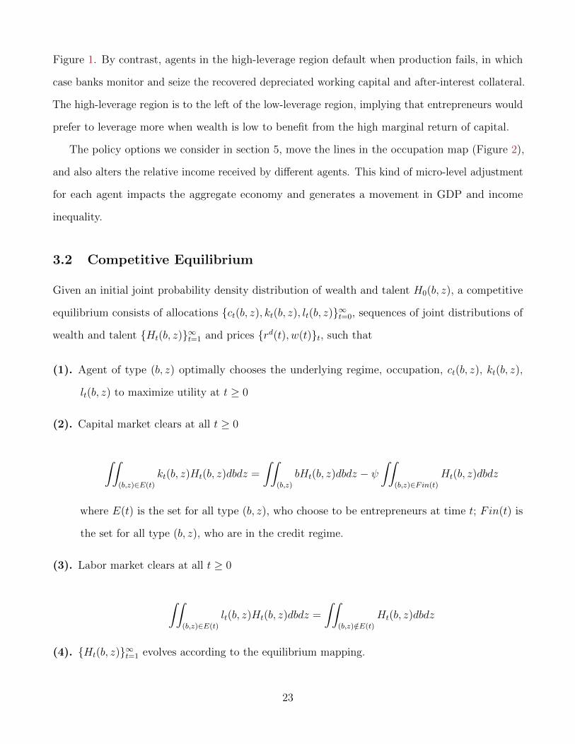
Figure 1. By contrast, agents in the high-leverage region default when production fails, in which

case banks monitor and seize the recovered depreciated working capital and after-interest collateral.

The high-leverage region is to the left of the low-leverage region, implying that entrepreneurs would

prefer to leverage more when wealth is low to benefit from the high marginal return of capital.

The policy options we consider in section 5, move the lines in the occupation map (Figure 2),

and also alters the relative income received by different agents. This kind of micro-level adjustment

for each agent impacts the aggregate economy and generates a movement in GDP and income

inequality.

3.2 Competitive Equilibrium

Given an initial joint probability density distribution of wealth and talent H0(b, z), a competitive

equilibrium consists of allocations ct(b, z), kt(b, z), lt(b, z)∞t=0, sequences of joint distributions of

wealth and talent Ht(b, z)∞t=1 and prices rd(t), w(t)t, such that

(1). Agent of type (b, z) optimally chooses the underlying regime, occupation, ct(b, z), kt(b, z),

lt(b, z) to maximize utility at t ≥ 0

(2). Capital market clears at all t ≥ 0

∫∫(b,z)∈E(t)

kt(b, z)Ht(b, z)dbdz =

∫∫(b,z)

bHt(b, z)dbdz − ψ∫∫

(b,z)∈Fin(t)

Ht(b, z)dbdz

where E(t) is the set for all type (b, z), who choose to be entrepreneurs at time t; Fin(t) is

the set for all type (b, z), who are in the credit regime.

(3). Labor market clears at all t ≥ 0

∫∫(b,z)∈E(t)

lt(b, z)Ht(b, z)dbdz =

∫∫(b,z)/∈E(t)

Ht(b, z)dbdz

(4). Ht(b, z)∞t=1 evolves according to the equilibrium mapping.

23

Ht+1(b, z)db = γµ(z)

∫z

1b′=bHt(b, z)dbdz + (1− γ)

∫b

1b′=bHt(b, z)db

where b′ is the bequest for agent of type (b, z), and 1b′=b is an indicator function which

equals 1 if b′ = b, and equals 0 otherwise.

The steady-state of the economy is defined as the invariant joint distribution of wealth and

talent H(b, z),

H(b, z) = limt→∞

Ht(b, z)

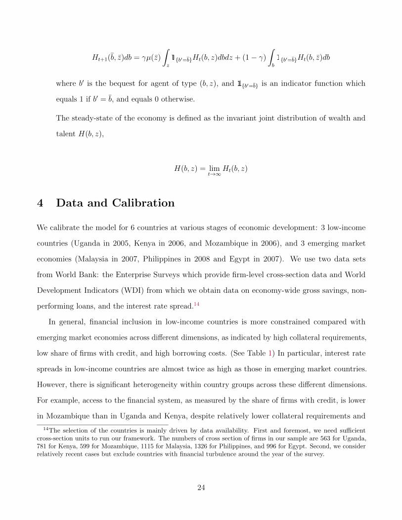
4 Data and Calibration

We calibrate the model for 6 countries at various stages of economic development: 3 low-income

countries (Uganda in 2005, Kenya in 2006, and Mozambique in 2006), and 3 emerging market

economies (Malaysia in 2007, Philippines in 2008 and Egypt in 2007). We use two data sets

from World Bank: the Enterprise Surveys which provide firm-level cross-section data and World

Development Indicators (WDI) from which we obtain data on economy-wide gross savings, non-

performing loans, and the interest rate spread.14

In general, financial inclusion in low-income countries is more constrained compared with

emerging market economies across different dimensions, as indicated by high collateral requirements,

low share of firms with credit, and high borrowing costs. (See Table 1) In particular, interest rate

spreads in low-income countries are almost twice as high as those in emerging market countries.

However, there is significant heterogeneity within country groups across these different dimensions.

For example, access to the financial system, as measured by the share of firms with credit, is lower

in Mozambique than in Uganda and Kenya, despite relatively lower collateral requirements and

14The selection of the countries is mainly driven by data availability. First and foremost, we need sufficientcross-section units to run our framework. The numbers of cross section of firms in our sample are 563 for Uganda,781 for Kenya, 599 for Mozambique, 1115 for Malaysia, 1326 for Philippines, and 996 for Egypt. Second, we considerrelatively recent cases but exclude countries with financial turbulence around the year of the survey.

24

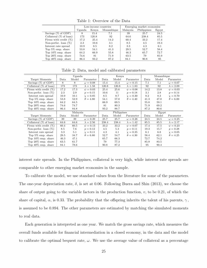
Table 1: Overview of the Data

Low-income countries Emerging market economiesUganda Kenya Mozambique Malaysia Philippines Egypt

Savings (% of GDP) 8 15.4 7.1 39 25.7 24.5Collateral (% of loan) 173 120.8 92 64.6 238.4 85.5Firms with credit (%) 17.2 25.4 14.2 60.4 33.2 17.4Non-perfor. loan (%) 2.3 10.6 3.1 8.5 4.5 19.3Interest rate spread 10.9 8.5 8.2 3.3 4.3 6.1Top 5% emp. share 53.8 54.1 41.3 29.5 52.7 58.4Top 10% emp. share 64.2 66.9 55.8 46.3 65.7 72.7Top 20% emp. share 74.6 81 71.9 63.5 79 85.9Top 40% emp. share 86.4 93.2 87.2 84.1 90.8 95

Table 2: Data, model and calibrated parameters

Uganda Kenya MozambiqueTarget Moments Data Model Parameter Data Model Parameter Data Model Parameter

Savings (% of GDP) 8 8 ω = 0.08 15.4 15.4 ω = 0.15 7.1 7.1 ω = 0.07Collateral (% of loan) 173 173 λ = 1.58 120.8 120.8 λ = 1.83 92 92 λ = 2.09Firms with credit (%) 17.2 17.3 ψ = 0.03 25.4 25.6 ψ = 0.08 14.2 13.8 ψ = 0.03Non-perfor. loan (%) 2.3 2.9 p = 0.15 10.6 11 p = 0.18 3.1 2.8 p = 0.14Interest rate spread 10.9 10.1 χ = 0.85 8.5 8.7 χ = 0.30 8.2 8.3 χ = 0.70Top 5% emp. share 53.8 52.9 θ = 4.80 54.1 57.0 θ = 4.40 41.3 47.0 θ = 6.00Top 10% emp. share 64.2 64.5 66.9 69.5 55.8 59.1Top 20% emp. share 74.6 74.7 81 80.3 71.9 69.2Top 40% emp. share 86.4 84.8 93.2 88.7 87.2 80.6

Malaysia Philippines EgyptTarget Moments Data Model Parameter Data Model Parameter Data Model Parameter

Savings (% of GDP) 39 39 ω = 0.39 25.7 25.7 ω = 0.26 24.5 24.5 ω = 0.25Collateral (% of loan) 64.6 64.6 λ = 2.56 238.4 238.4 λ = 1.42 85.5 85.5 λ = 2.17Firms with credit (%) 60.4 60.5 ψ = 0.13 33.2 33.2 ψ = 0.07 17.4 17.5 ψ = 0.23Non-perfor. loan (%) 8.5 7.6 p = 0.12 4.5 5.3 p = 0.11 19.3 15.7 p = 0.28Interest rate spread 3.3 5.1 χ = 0.11 4.3 4.1 χ = 0.35 6.1 6.8 χ = 0.05Top 5% emp. share 29.5 34.7 θ = 6.80 52.7 54.7 θ = 4.30 58.4 62.1 θ = 4.25Top 10% emp. share 46.3 47.1 65.7 66.3 72.7 74.2Top 20% emp. share 63.5 61.7 79 77.3 85.9 83.5Top 40% emp. share 84.1 78.6 90.8 87.2 95 90.4

interest rate spreads. In the Philippines, collateral is very high, while interest rate spreads are

comparable to other emerging market economies in the sample.

To calibrate the model, we use standard values from the literature for some of the parameters.

The one-year depreciation rate, δ, is set at 0.06. Following Buera and Shin (2013), we choose the

share of output going to the variable factors in the production function, v, to be 0.21, of which the

share of capital, α, is 0.33. The probability that the offspring inherits the talent of his parents, γ ,

is assumed to be 0.894. The other parameters are estimated by matching the simulated moments

to real data.

Each generation is interpreted as one year. We match the gross savings rate, which measures the

overall funds available for financial intermediation in a closed economy, in the data and the model

to calibrate the optimal bequest rate, ω. We use the average value of collateral as a percentage

25

of the loan to calibrate the parameter λ, which captures the degree of financial friction caused by

limited commitment. The financial participation cost, ψ, intermediation cost, χ, the probability of

failure, p and the parameter governing the talent distribution, θ are jointly calibrated to match the

moments of the percent of firms with a line of credit, non-performing loans (NPLs) as a percentage

of total loans, interest rate spreads, and the employment share distribution (using four brackets of

employment shares—top 5% / 10% /20% / 40%). Even though parameters ψ, χ, p and θ affect

the value of all these moments, and are jointly calibrated, each moment is primarily affected by

some particular parameters. Specifically, the moment of percent of firms with credit is mostly

determined by the credit participation cost ψ. Increasing the value of ψ increases the percent of

firms with credit. The non-performing loan ratio and interest rates are determined by parameters

χ, and p. However, the relationships are non-monotonic for some parameter values. For example,

when the probability of project failure p increases, if the entrepreneurs’ leverage ratio is unchanged,

the non-performing loan ratio and interest rate spread should increase. However, the higher p

may reduce the leverage ratio due to higher monitoring costs, which results in fewer defaults,

and, thereby a lower non-performing loan ratio and interest rate spreads. The employment share

distribution is matched primarily by adjusting the value of parameter θ, which governs the shape

of the entrepreneurial talent distribution. Note that the parameter η may not be well identified

for some countries, because to some extent it has a similar impact on all the moments as the

parameter p. The way we calibrate parameter η is to set its value close to but below (λ−1)(1+rd)λ(1−δ) , so

that the moments of interest rate spread and the non-performing loan ratio are most sensitive to

parameters p and χ.15 In this sense, the parameter η could be regarded as a scale parameter, which

is important for us to calibrate the other parameters and match the moments. To best match the

empirical moments, we set η at 0.37 for Uganda, Kenya and Malaysia, 0.54 for Mozambique, 0.29

for Philippines, and 0.44 for Egypt.

From Table 2, it is clear that the model performs well in terms of matching the macroeconomic

moments. The percent of firms with credit generated by the model is almost exactly matched with

15In a more technical version of this paper, we prove that if η is set larger than (λ−1)(1+rd)λ(1−δ) , there would be no

default in the economy because all entrepreneurs choose to have a low leverage ratio. The technical version isavailable upon request.

26

that in the data for all six countries. The NPLs ratio and interest rate spread are matched well,

although some countries have high low NPLs ratio but a relatively low interest rate spread (e.g.

Maylasia and Egypt) while other countries have NPL ratios and a high interest rate spread (e.g.

Uganda and Mozambique). The employment share distribution is also captured, but in general

the model tends to generate more larger firms compared to the data (larger value for top 5%

employment share and a lower value for the 40% employment share).

The linkages between different characteristics of an economy and financial inclusion are complex.

For example, it might seem surprising that the calibrated financial participation cost, ψ, in general,

is lower in low-income countries despite the lower financial inclusion ratio. However, both λ and χ

affect the financial inclusion ratio in the model—a higher λ and lower χ increases the participation

cost in emerging market countries. Moreover, these countries have higher saving rates (higher ω),

which implies that agents transfer more wealth to the next generation. In this case, the credit

participation cost is a relatively smaller proportion of the agents’ wealth in emerging market

countries, and, therefore, is less binding, as reflected in the high financial inclusion ratio. In the

next section, we analyze the implications of financial inclusion on the economy and identify the role

that country characteristics play in the process.

Since agents in our model have myopic savings rate (or a constant bequest rate to the offspring),

our calibration strategy departs from the standard of literature in two ways. First, we calibrate the

tightness of the borrowing constraint (parameter λ) directly from the average value of collateral as a

percentage of the loan, which is available from the enterprise survey. This is reasonable because the

parameter λ governs the tightness of the borrowing constraint, which affects the value of collateral

held by firms.16 In Buera and Shin (2013), this parameter is calibrated to match the credit to GDP

ratio. We do not follow Buera and Shin (2013) because the myopic savings assumption prevents

us from generating a wide range of the credit to GDP ratio to match the statistic in all countries.

In fact, with the calibrated parameters, our model generates lower credit to GDP ratios by about

16In our model, parameter λ refers to the maximum leverage ratio, or the minimum value of collateral held as apercentage of the loan. We calibrate this parameter from the average instead of the minimum value of collateral as apercentage of the loan, because some firms in the data post no collateral while borrowing. Calibration based on theminimum value would imply λ = +∞, which is not reasonable.

27

10%− 40% compared with those in the data. This is because with myopic savings rate, agents do

not disave when borrowing constraints are relaxed, as in Buera et al. (2011). Second, following

Gine and Townsend (2004), we calibrate the savings rate, ω, directly from the actual data on

gross savings rate. As a result, the model fails to match the level of deposit interest rate, which

is a prevalent problem for all myopic-agent models without a time discount factor (and thus an

endogenous savings rate). The failure to match the deposit interest rate does change the predicted

level of the Gini coefficient. However, it doesn’t alter the trend of Gini when financial reform

policies are evaluated.

5 Evaluation of Policy Options

As mentioned above, financial inclusion is reflected by three parameters in our model. The credit

participation cost, ψ, directly measures the difficulty of obtaining credit. An increase in this ratio

therefore reflects greater financial access. The parameter λ in the borrowing constraint coincides

directly with the maximum leverage ratio, an increase in which reflects lower collateral requirements.

Finally, a decrease in the cost of state verification, χ, indicates an increase in the ”efficiency” of

financial intermediation. It should be noted that in our model, the percent of firms with credit is

endogenous and is affected by the three parameters above.

Because financial inclusion is multidimensional, it is difficult to identify precisely the meaning

of these three parameters from an empirical standpoint. However, one can find evidence of policies

that address one dimension or the other. For example, Assuncao et al. (2012) and Alem and

Townsend (2013) find that the distance to a bank branch matters for credit access, which suggests

that policies that promote branch openings in rural, unbanked locations would help reduce the credit

participation cost, ψ.17 Moreover, during the recent financial crisis, many countries widened the

range of securities that would be accepted as collateral with the aim of boosting lending to companies

and households. This reflects an increase in λ in our model. Finally, financial liberalization and the

17Many developing countries have conducted such kind of policies. For example, after a bank nationalization in1969, the Indian government launched an ambitious social banking program which sought to improve the access ofthe rural poor to formal credit and saving opportunities (Burgess and Pande, 2005).

28

resultant competition between financial institutions could accelerate investment in computerization,

thereby improving the efficiency of intermediation (reflected by a decrease in χ in our model). For

example, from 1985 to 1994, the Thail banking sector had become a more capital-intensive industry,

substituting phisical capital for labor. The average cost of raising funds decreased from 14.40% in

1985 to 5.61% in 1994 for large-sized banks (Okuda and Mieno, 1999).

This section analyzes the policy implications of promoting financial inclusion across these three

dimensions for the countries in our sample. Specifically, we focus on changes in the steady states of

the economy when these parameters change.18 Figures 3 – 8 below present the simulation results

when each of the three financial parameters changes separately (on the horizontal axis). For all the

following experiments, we measure inequality with the Gini coefficient. GDP is measured as the

sum of all individual incomes. We follow Buera and Shin (2013), and measure the model implied

TFP as Y/(KαL1−α), where Y is aggregate output, K is aggregate capital, and L is the size of

labor force. We use circles in the figure to pin point the position of countries in the survey dates.

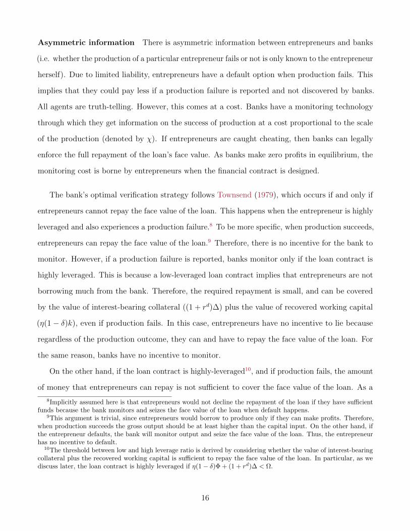
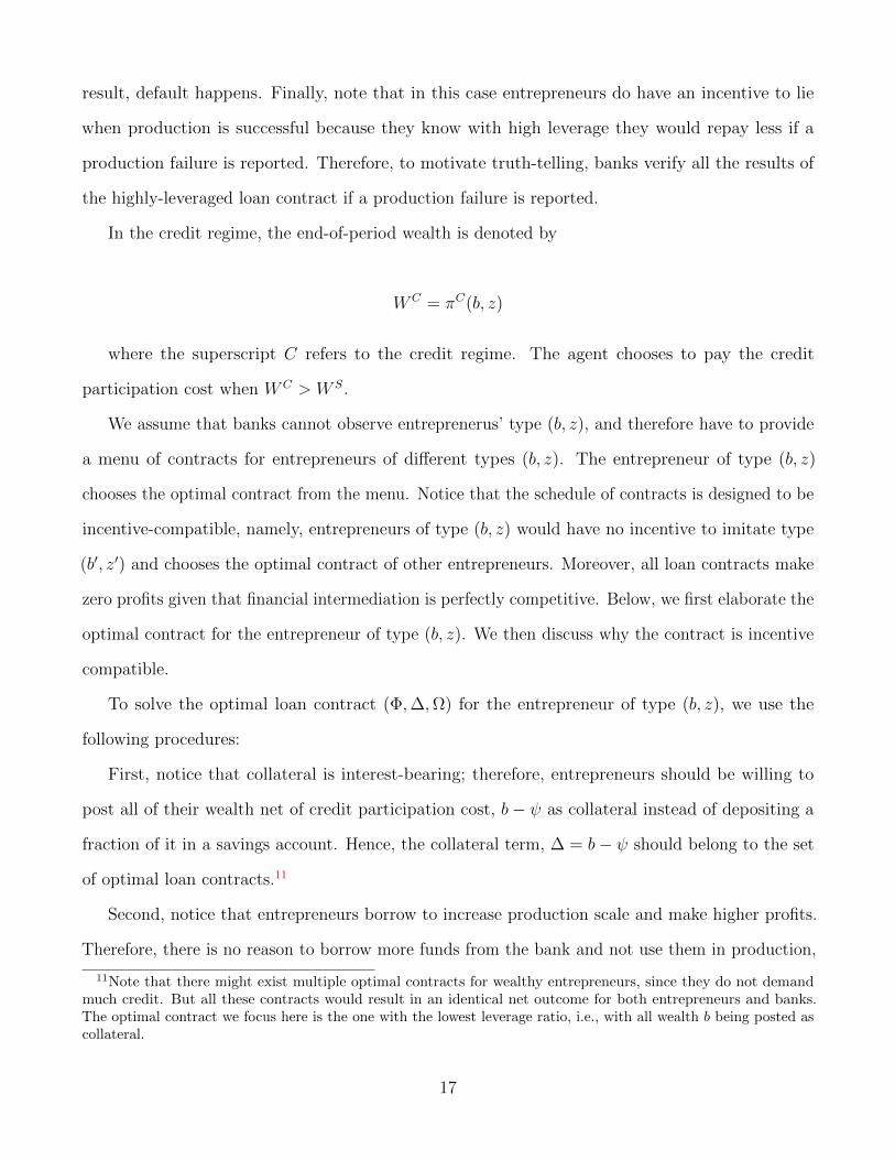
5.1 Reducing the participation cost

Figure 3 – Figure 4 present the impact of a decline in the credit participation cost ψ from 0.15

to 0 (moving from left to right). A decrease in the participation cost pushes up GDP through its

positive impact on investment for two reasons. First, a lower financial participation cost enables

more firms to have access to credit, leading to more capital invested in production. Second, less

funds are wasted in unproductive contract negotiation and, hence, firms can invest more capital in

production. TFP increases as capital is more efficiently allocated among entrepreneurs.

The interest rate spread is stable when ψ is high, but eventually decreases in some countries

(Uganda, Mozambique, and Philippines) and increases slightly in others (e.g. in Kenya and Malaysia).

18Note that it takes time for the economy to transition from one steady state to another when these parameterschange. The transitional dynamics are also computable from the model. However, we only report the outcome ofsimulations in steady states because focusing on the transitional dynamics could be misleading for two reasons:(1) the transition is rapid at the beginning but becomes slower when the economy is approaching the steady state.This is inconsistent with reality, where the impact of financial reforms happens gradually, or at least the immediateimpact is not significant; (2) the numerical error is large relative to that in the steady state, possibly leading toovershooting of some variables if parameters are adjusted a lot. These two problems associated with transitionaldynamics exist for all quantitative macroeconomic models, although the first problem could be mitigated to someextent if agents were modeled as forward-looking.

29

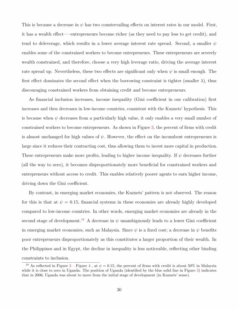
This is because a decrease in ψ has two countervailing effects on interest rates in our model. First,

it has a wealth effect—–entrepreneurs become richer (as they need to pay less to get credit), and

tend to deleverage, which results in a lower average interest rate spread. Second, a smaller ψ

enables some of the constrained workers to become entrepreneurs. These entrepreneurs are severely

wealth constrained, and therefore, choose a very high leverage ratio, driving the average interest

rate spread up. Nevertheless, these two effects are significant only when ψ is small enough. The

first effect dominates the second effect when the borrowing constraint is tighter (smaller λ), thus

discouraging constrained workers from obtaining credit and become entrepreneurs.

As financial inclusion increases, income inequality (Gini coefficient in our calibration) first

increases and then decreases in low-income countries, consistent with the Kuznets’ hypothesis. This

is because when ψ decreases from a particularly high value, it only enables a very small number of

constrained workers to become entrepreneurs. As shown in Figure 3, the percent of firms with credit

is almost unchanged for high values of ψ. However, the effect on the incumbent entrepreneurs is

large since it reduces their contracting cost, thus allowing them to invest more capital in production.

These entrepreneurs make more profits, leading to higher income inequality. If ψ decreases further

(all the way to zero), it becomes disproportionately more beneficial for constrained workers and

entrepreneurs without access to credit. This enables relatively poorer agents to earn higher income,

driving down the Gini coefficient.

By contrast, in emerging market economies, the Kuznets’ pattern is not observed. The reason

for this is that at ψ = 0.15, financial systems in these economies are already highly developed

compared to low-income countries. In other words, emerging market economies are already in the

second stage of development.19 A decrease in ψ unambiguously leads to a lower Gini coefficient

in emerging market economies, such as Malaysia. Since ψ is a fixed cost; a decrease in ψ benefits

poor entrepreneurs disproportionately as this constitutes a larger proportion of their wealth. In

the Philippines and in Egypt, the decline in inequality is less noticeable, reflecting other binding

constraints to inclusion.

19 As reflected in Figure 3 – Figure 4 , at ψ = 0.15, the percent of firms with credit is about 50% in Malaysiawhile it is close to zero in Uganda. The position of Uganda (identified by the blue solid line in Figure 3) indicatesthat in 2006, Uganda was about to move from the initial stage of development (in Kuznets’ sense).

30

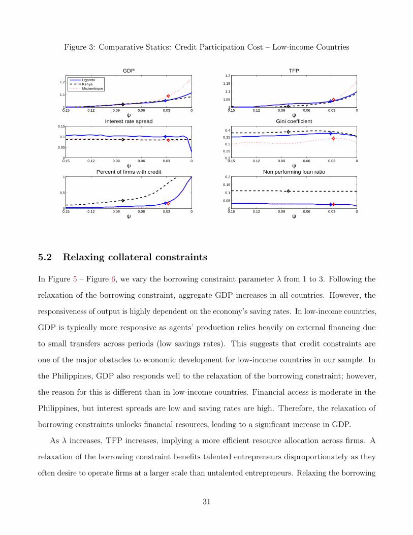
Figure 3: Comparative Statics: Credit Participation Cost – Low-income Countries

00.030.060.090.120.151

1.1

1.2

GDP

ψ

UgandaKenyaMozambique

00.030.060.090.120.151

1.05

1.1

1.15

1.2TFP

ψ

00.030.060.090.120.150

0.05

0.1

0.15Interest rate spread

ψ00.030.060.090.120.15

0.2

0.25

0.3

0.35

0.4

Gini coefficient

ψ

00.030.060.090.120.150

0.5

1Percent of firms with credit

ψ00.030.060.090.120.15

0

0.05

0.1

0.15

0.2Non performing loan ratio

ψ

5.2 Relaxing collateral constraints

In Figure 5 – Figure 6, we vary the borrowing constraint parameter λ from 1 to 3. Following the

relaxation of the borrowing constraint, aggregate GDP increases in all countries. However, the

responsiveness of output is highly dependent on the economy’s saving rates. In low-income countries,

GDP is typically more responsive as agents’ production relies heavily on external financing due

to small transfers across periods (low savings rates). This suggests that credit constraints are

one of the major obstacles to economic development for low-income countries in our sample. In

the Philippines, GDP also responds well to the relaxation of the borrowing constraint; however,

the reason for this is different than in low-income countries. Financial access is moderate in the

Philippines, but interest spreads are low and saving rates are high. Therefore, the relaxation of

borrowing constraints unlocks financial resources, leading to a significant increase in GDP.

As λ increases, TFP increases, implying a more efficient resource allocation across firms. A

relaxation of the borrowing constraint benefits talented entrepreneurs disproportionately as they

often desire to operate firms at a larger scale than untalented entrepreneurs. Relaxing the borrowing

31

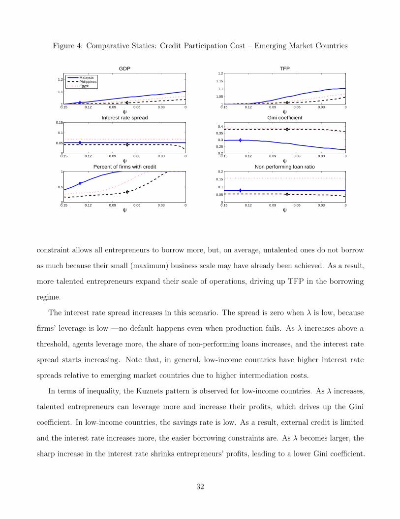
Figure 4: Comparative Statics: Credit Participation Cost – Emerging Market Countries

00.030.060.090.120.151

1.1

1.2

GDP

ψ

MalaysiaPhilippinesEgypt

00.030.060.090.120.151

1.05

1.1

1.15

1.2TFP

ψ

00.030.060.090.120.150

0.05

0.1

0.15Interest rate spread

ψ00.030.060.090.120.15

0.2

0.25

0.3

0.35

0.4

Gini coefficient

ψ

00.030.060.090.120.150

0.5

1Percent of firms with credit

ψ00.030.060.090.120.15

0

0.05

0.1

0.15

0.2Non performing loan ratio

ψ

constraint allows all entrepreneurs to borrow more, but, on average, untalented ones do not borrow

as much because their small (maximum) business scale may have already been achieved. As a result,

more talented entrepreneurs expand their scale of operations, driving up TFP in the borrowing

regime.

The interest rate spread increases in this scenario. The spread is zero when λ is low, because

firms’ leverage is low —no default happens even when production fails. As λ increases above a

threshold, agents leverage more, the share of non-performing loans increases, and the interest rate

spread starts increasing. Note that, in general, low-income countries have higher interest rate

spreads relative to emerging market countries due to higher intermediation costs.

In terms of inequality, the Kuznets pattern is observed for low-income countries. As λ increases,

talented entrepreneurs can leverage more and increase their profits, which drives up the Gini

coefficient. In low-income countries, the savings rate is low. As a result, external credit is limited

and the interest rate increases more, the easier borrowing constraints are. As λ becomes larger, the

sharp increase in the interest rate shrinks entrepreneurs’ profits, leading to a lower Gini coefficient.

32

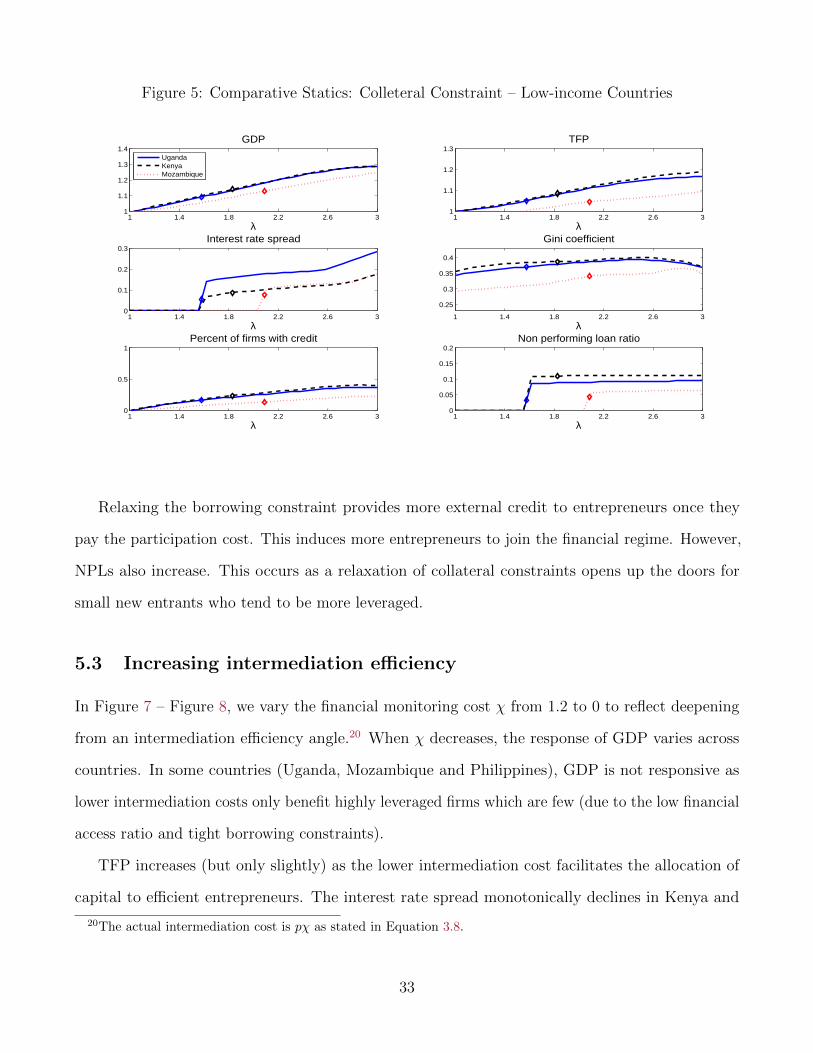
Figure 5: Comparative Statics: Colleteral Constraint – Low-income Countries

1 1.4 1.8 2.2 2.6 31

1.1

1.2

1.3

1.4GDP

λ

UgandaKenyaMozambique

1 1.4 1.8 2.2 2.6 31

1.1

1.2

1.3TFP

λ

1 1.4 1.8 2.2 2.6 30

0.1

0.2

0.3Interest rate spread

λ1 1.4 1.8 2.2 2.6 3

0.25

0.3

0.35

0.4

Gini coefficient

λ

1 1.4 1.8 2.2 2.6 30

0.5

1Percent of firms with credit

λ1 1.4 1.8 2.2 2.6 3

0

0.05

0.1

0.15

0.2Non performing loan ratio

λ

Relaxing the borrowing constraint provides more external credit to entrepreneurs once they

pay the participation cost. This induces more entrepreneurs to join the financial regime. However,

NPLs also increase. This occurs as a relaxation of collateral constraints opens up the doors for

small new entrants who tend to be more leveraged.

5.3 Increasing intermediation efficiency

In Figure 7 – Figure 8, we vary the financial monitoring cost χ from 1.2 to 0 to reflect deepening

from an intermediation efficiency angle.20 When χ decreases, the response of GDP varies across

countries. In some countries (Uganda, Mozambique and Philippines), GDP is not responsive as

lower intermediation costs only benefit highly leveraged firms which are few (due to the low financial

access ratio and tight borrowing constraints).

TFP increases (but only slightly) as the lower intermediation cost facilitates the allocation of

capital to efficient entrepreneurs. The interest rate spread monotonically declines in Kenya and

20The actual intermediation cost is pχ as stated in Equation 3.8.

33

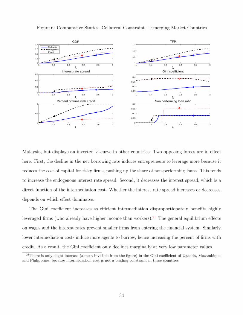
Figure 6: Comparative Statics: Collateral Constraint – Emerging Market Countries

1 1.4 1.8 2.2 2.6 31

1.1

1.2

1.3

1.4GDP

λ

MalaysiaPhilippinesEgypt

1 1.4 1.8 2.2 2.6 31

1.1

1.2

1.3TFP

λ

1 1.4 1.8 2.2 2.6 30

0.1

0.2

0.3Interest rate spread

λ1 1.4 1.8 2.2 2.6 3

0.25

0.3

0.35

0.4

Gini coefficient

λ

1 1.4 1.8 2.2 2.6 30

0.5

1Percent of firms with credit

λ1 1.4 1.8 2.2 2.6 3

0

0.05

0.1

0.15

0.2Non performing loan ratio

λ

Malaysia, but displays an inverted V -curve in other countries. Two opposing forces are in effect

here. First, the decline in the net borrowing rate induces entrepreneurs to leverage more because it

reduces the cost of capital for risky firms, pushing up the share of non-performing loans. This tends

to increase the endogenous interest rate spread. Second, it decreases the interest spread, which is a

direct function of the intermediation cost. Whether the interest rate spread increases or decreases,

depends on which effect dominates.

The Gini coefficient increases as efficient intermediation disproportionately benefits highly

leveraged firms (who already have higher income than workers).21 The general equilibrium effects

on wages and the interest rates prevent smaller firms from entering the financial system. Similarly,

lower intermediation costs induce more agents to borrow, hence increasing the percent of firms with

credit. As a result, the Gini coefficient only declines marginally at very low parameter values.

21There is only slight increase (almost invisible from the figure) in the Gini coefficient of Uganda, Mozambique,and Philippines, because intermediation cost is not a binding constraint in these countries.

34

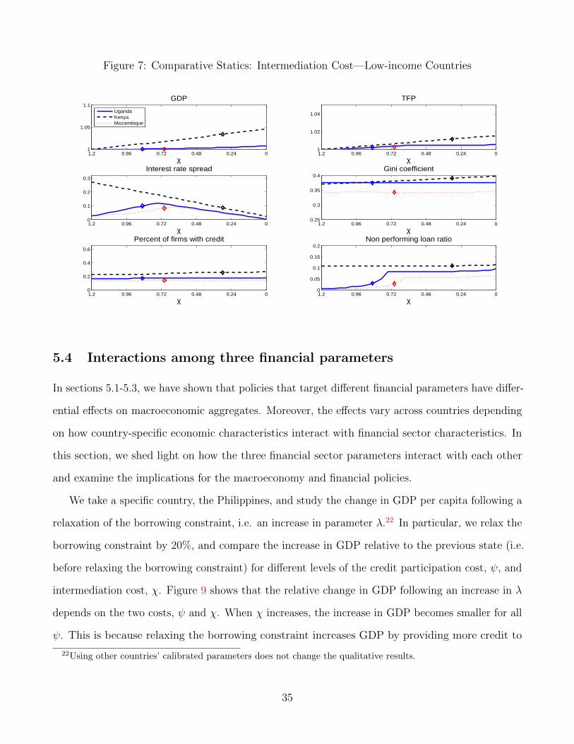
Figure 7: Comparative Statics: Intermediation Cost—Low-income Countries

00.240.480.720.961.21

1.05

1.1GDP

χ

UgandaKenyaMozambique

00.240.480.720.961.21

1.02

1.04

TFP

χ

00.240.480.720.961.20

0.1

0.2

0.3

Interest rate spread

χ00.240.480.720.961.2

0.25

0.3

0.35

0.4Gini coefficient

χ

00.240.480.720.961.20

0.2

0.4

0.6

Percent of firms with credit

χ00.240.480.720.961.2

0

0.05

0.1

0.15

0.2Non performing loan ratio

χ

5.4 Interactions among three financial parameters

In sections 5.1-5.3, we have shown that policies that target different financial parameters have differ-

ential effects on macroeconomic aggregates. Moreover, the effects vary across countries depending

on how country-specific economic characteristics interact with financial sector characteristics. In

this section, we shed light on how the three financial sector parameters interact with each other

and examine the implications for the macroeconomy and financial policies.

We take a specific country, the Philippines, and study the change in GDP per capita following a

relaxation of the borrowing constraint, i.e. an increase in parameter λ.22 In particular, we relax the

borrowing constraint by 20%, and compare the increase in GDP relative to the previous state (i.e.

before relaxing the borrowing constraint) for different levels of the credit participation cost, ψ, and

intermediation cost, χ. Figure 9 shows that the relative change in GDP following an increase in λ

depends on the two costs, ψ and χ. When χ increases, the increase in GDP becomes smaller for all

ψ. This is because relaxing the borrowing constraint increases GDP by providing more credit to

22Using other countries’ calibrated parameters does not change the qualitative results.

35

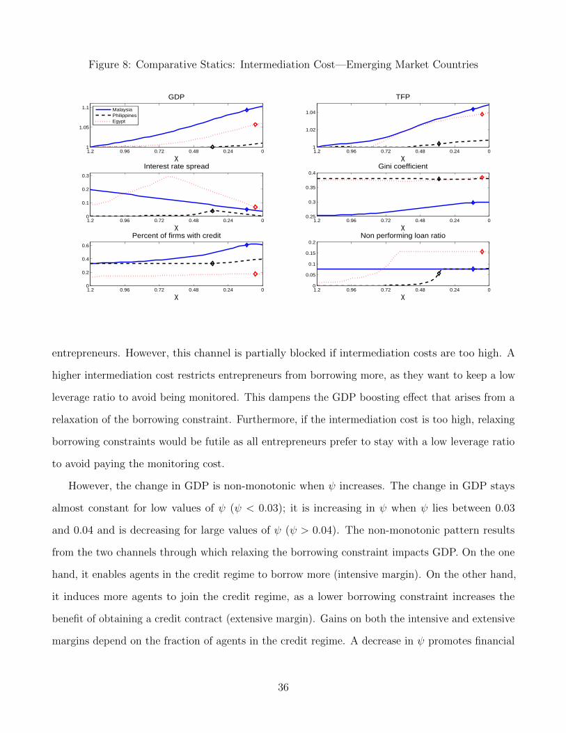
Figure 8: Comparative Statics: Intermediation Cost—Emerging Market Countries

00.240.480.720.961.21

1.05

1.1

GDP

χ

MalaysiaPhilippinesEgypt

00.240.480.720.961.21

1.02

1.04

TFP

χ

00.240.480.720.961.20

0.1

0.2

0.3

Interest rate spread

χ00.240.480.720.961.2

0.25

0.3

0.35

0.4Gini coefficient

χ

00.240.480.720.961.20

0.2

0.4

0.6

Percent of firms with credit

χ00.240.480.720.961.2

0

0.05

0.1

0.15

0.2Non performing loan ratio

χ

entrepreneurs. However, this channel is partially blocked if intermediation costs are too high. A

higher intermediation cost restricts entrepreneurs from borrowing more, as they want to keep a low

leverage ratio to avoid being monitored. This dampens the GDP boosting effect that arises from a

relaxation of the borrowing constraint. Furthermore, if the intermediation cost is too high, relaxing

borrowing constraints would be futile as all entrepreneurs prefer to stay with a low leverage ratio

to avoid paying the monitoring cost.

However, the change in GDP is non-monotonic when ψ increases. The change in GDP stays

almost constant for low values of ψ (ψ < 0.03); it is increasing in ψ when ψ lies between 0.03

and 0.04 and is decreasing for large values of ψ (ψ > 0.04). The non-monotonic pattern results

from the two channels through which relaxing the borrowing constraint impacts GDP. On the one

hand, it enables agents in the credit regime to borrow more (intensive margin). On the other hand,

it induces more agents to join the credit regime, as a lower borrowing constraint increases the

benefit of obtaining a credit contract (extensive margin). Gains on both the intensive and extensive

margins depend on the fraction of agents in the credit regime. A decrease in ψ promotes financial

36

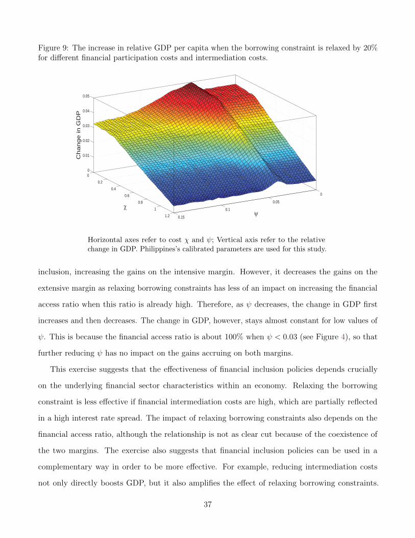
Figure 9: The increase in relative GDP per capita when the borrowing constraint is relaxed by 20%for different financial participation costs and intermediation costs.

0

0.05

0.1

0.15

0

0.2

0.4

0.6

0.8

1

1.2

0

0.01

0.02

0.03

0.04

0.05

Change in G

DP

Horizontal axes refer to cost χ and ψ; Vertical axis refer to the relativechange in GDP. Philippines’s calibrated parameters are used for this study.

inclusion, increasing the gains on the intensive margin. However, it decreases the gains on the

extensive margin as relaxing borrowing constraints has less of an impact on increasing the financial

access ratio when this ratio is already high. Therefore, as ψ decreases, the change in GDP first

increases and then decreases. The change in GDP, however, stays almost constant for low values of

ψ. This is because the financial access ratio is about 100% when ψ < 0.03 (see Figure 4), so that

further reducing ψ has no impact on the gains accruing on both margins.

This exercise suggests that the effectiveness of financial inclusion policies depends crucially

on the underlying financial sector characteristics within an economy. Relaxing the borrowing

constraint is less effective if financial intermediation costs are high, which are partially reflected

in a high interest rate spread. The impact of relaxing borrowing constraints also depends on the

financial access ratio, although the relationship is not as clear cut because of the coexistence of

the two margins. The exercise also suggests that financial inclusion policies can be used in a

complementary way in order to be more effective. For example, reducing intermediation costs

not only directly boosts GDP, but it also amplifies the effect of relaxing borrowing constraints.

37

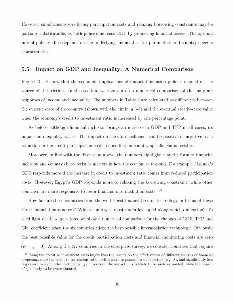
However, simultaneously reducing participation costs and relaxing borrowing constraints may be

partially substitutable, as both policies increase GDP by promoting financial access. The optimal

mix of policies thus depends on the underlying financial sector parameters and country-specific

characteristics.

5.5 Impact on GDP and Inequality: A Numerical Comparison

Figures 3 – 8 show that the economic implications of financial inclusion policies depend on the

source of the friction. In this section, we zoom-in on a numerical comparison of the marginal

responses of income and inequality. The numbers in Table 3 are calculated as differences between

the current state of the country (shown with the circle in 3-8) and the eventual steady-state value

when the economy’s credit to investment ratio is increased by one percentage point.

As before, although financial inclusion brings an increase in GDP and TFP in all cases, its

impact on inequality varies. The impact on the Gini coefficient can be positive or negative for a

reduction in the credit participation costs, depending on country specific characteristics.

Moreover, in line with the discussion above, the numbers highlight that the form of financial

inclusion and country characteristics matters in how the economies respond. For example, Uganda’s

GDP responds more if the increase in credit to investment ratio comes from reduced participation

costs. However, Egypt’s GDP responds more to relaxing the borrowing constraint; while other

countries are more responsive to lower financial intermediation costs. 23

How far are these countries from the world best financial sector technology in terms of these

three financial parameters? Which country is most underdeveloped along which dimension? To

shed light on these questions, we show a numerical comparison for the changes of GDP, TFP and

Gini coefficient when the six countries adopt the best-possible intermediation technology. Obviously,

the best possible value for the credit participation costs and financial monitoring costs are zero

(ψ = χ = 0). Among the 127 countries in the enterprise survey, we consider countries that require

23Using the credit to investment ratio might bias the results on the effectiveness of different sources of financialdeepening, since the credit to investment ratio itself is more responsive to some factors (e.g. λ), and significantly lessresponsive to some other factor (e.g. χ). Therefore, the impact of λ is likely to be underestimated, while the impactof χ is likely to be overestimated.

38

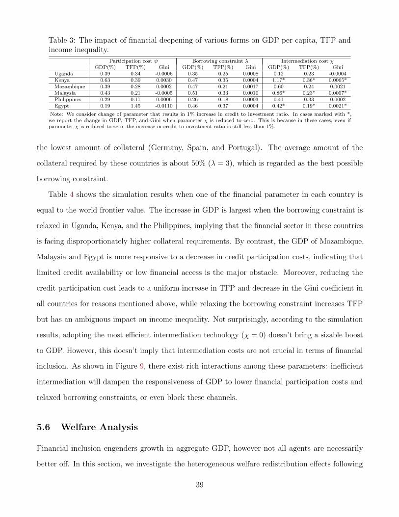
Table 3: The impact of financial deepening of various forms on GDP per capita, TFP andincome inequality.

Participation cost ψ Borrowing constraint λ Intermediation cost χGDP(%) TFP(%) Gini GDP(%) TFP(%) Gini GDP(%) TFP(%) Gini

Uganda 0.39 0.34 -0.0006 0.35 0.25 0.0008 0.12 0.23 -0.0004Kenya 0.63 0.39 0.0030 0.47 0.35 0.0004 1.17* 0.36* 0.0065*Mozambique 0.39 0.28 0.0002 0.47 0.21 0.0017 0.60 0.24 0.0021Malaysia 0.43 0.21 -0.0005 0.51 0.33 0.0010 0.86* 0.23* 0.0007*Philippines 0.29 0.17 0.0006 0.26 0.18 0.0003 0.41 0.33 0.0002Egypt 0.19 1.45 -0.0110 0.46 0.37 0.0004 0.42* 0.19* 0.0021*

Note: We consider change of parameter that results in 1% increase in credit to investment ratio. In cases marked with *,we report the change in GDP, TFP, and Gini when parameter χ is reduced to zero. This is because in these cases, even ifparameter χ is reduced to zero, the increase in credit to investment ratio is still less than 1%.

the lowest amount of collateral (Germany, Spain, and Portugal). The average amount of the

collateral required by these countries is about 50% (λ = 3), which is regarded as the best possible

borrowing constraint.

Table 4 shows the simulation results when one of the financial parameter in each country is

equal to the world frontier value. The increase in GDP is largest when the borrowing constraint is

relaxed in Uganda, Kenya, and the Philippines, implying that the financial sector in these countries

is facing disproportionately higher collateral requirements. By contrast, the GDP of Mozambique,

Malaysia and Egypt is more responsive to a decrease in credit participation costs, indicating that

limited credit availability or low financial access is the major obstacle. Moreover, reducing the

credit participation cost leads to a uniform increase in TFP and decrease in the Gini coefficient in

all countries for reasons mentioned above, while relaxing the borrowing constraint increases TFP

but has an ambiguous impact on income inequality. Not surprisingly, according to the simulation

results, adopting the most efficient intermediation technology (χ = 0) doesn’t bring a sizable boost

to GDP. However, this doesn’t imply that intermediation costs are not crucial in terms of financial

inclusion. As shown in Figure 9, there exist rich interactions among these parameters: inefficient

intermediation will dampen the responsiveness of GDP to lower financial participation costs and

relaxed borrowing constraints, or even block these channels.

5.6 Welfare Analysis

Financial inclusion engenders growth in aggregate GDP, however not all agents are necessarily

better off. In this section, we investigate the heterogeneous welfare redistribution effects following

39

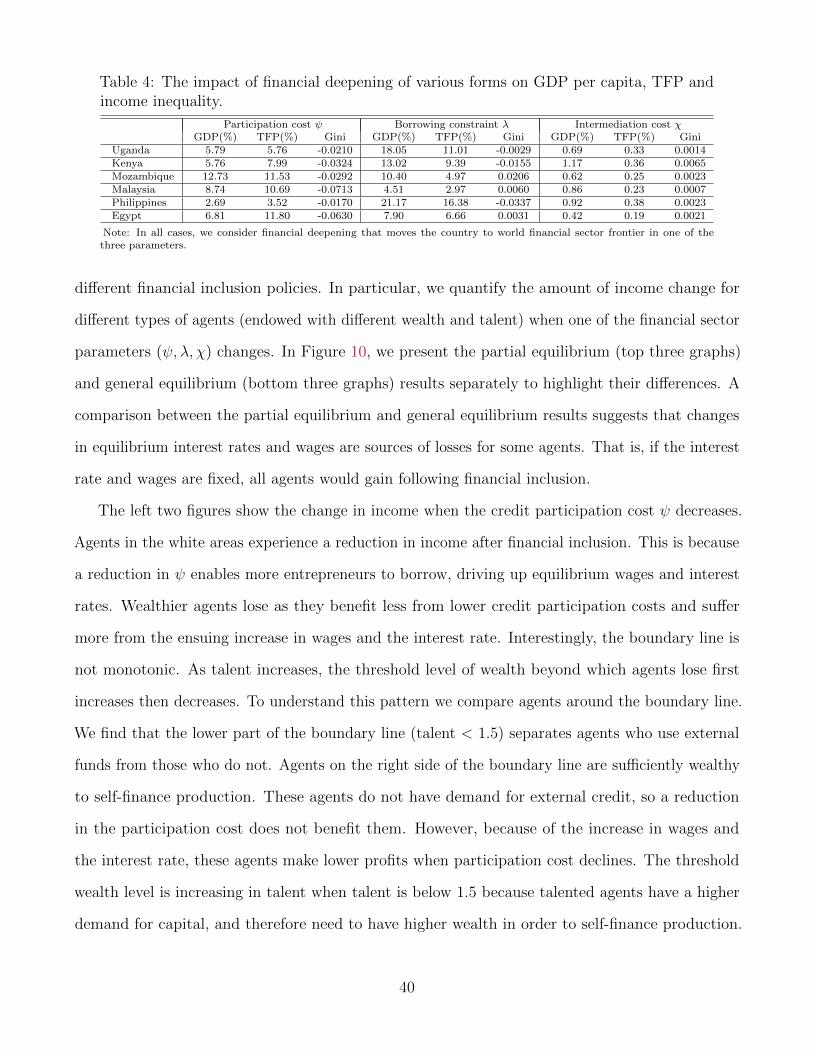
Table 4: The impact of financial deepening of various forms on GDP per capita, TFP andincome inequality.

Participation cost ψ Borrowing constraint λ Intermediation cost χGDP(%) TFP(%) Gini GDP(%) TFP(%) Gini GDP(%) TFP(%) Gini

Uganda 5.79 5.76 -0.0210 18.05 11.01 -0.0029 0.69 0.33 0.0014Kenya 5.76 7.99 -0.0324 13.02 9.39 -0.0155 1.17 0.36 0.0065Mozambique 12.73 11.53 -0.0292 10.40 4.97 0.0206 0.62 0.25 0.0023Malaysia 8.74 10.69 -0.0713 4.51 2.97 0.0060 0.86 0.23 0.0007Philippines 2.69 3.52 -0.0170 21.17 16.38 -0.0337 0.92 0.38 0.0023Egypt 6.81 11.80 -0.0630 7.90 6.66 0.0031 0.42 0.19 0.0021

Note: In all cases, we consider financial deepening that moves the country to world financial sector frontier in one of thethree parameters.

different financial inclusion policies. In particular, we quantify the amount of income change for

different types of agents (endowed with different wealth and talent) when one of the financial sector

parameters (ψ, λ, χ) changes. In Figure 10, we present the partial equilibrium (top three graphs)

and general equilibrium (bottom three graphs) results separately to highlight their differences. A

comparison between the partial equilibrium and general equilibrium results suggests that changes

in equilibrium interest rates and wages are sources of losses for some agents. That is, if the interest

rate and wages are fixed, all agents would gain following financial inclusion.

The left two figures show the change in income when the credit participation cost ψ decreases.

Agents in the white areas experience a reduction in income after financial inclusion. This is because

a reduction in ψ enables more entrepreneurs to borrow, driving up equilibrium wages and interest

rates. Wealthier agents lose as they benefit less from lower credit participation costs and suffer

more from the ensuing increase in wages and the interest rate. Interestingly, the boundary line is

not monotonic. As talent increases, the threshold level of wealth beyond which agents lose first

increases then decreases. To understand this pattern we compare agents around the boundary line.

We find that the lower part of the boundary line (talent < 1.5) separates agents who use external

funds from those who do not. Agents on the right side of the boundary line are sufficiently wealthy

to self-finance production. These agents do not have demand for external credit, so a reduction

in the participation cost does not benefit them. However, because of the increase in wages and

the interest rate, these agents make lower profits when participation cost declines. The threshold

wealth level is increasing in talent when talent is below 1.5 because talented agents have a higher

demand for capital, and therefore need to have higher wealth in order to self-finance production.

40

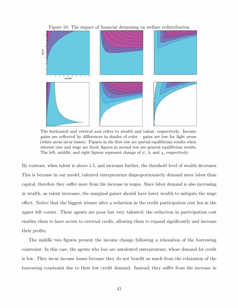
Figure 10: The impact of financial deepening on welfare redistribution.

tale

nt

0 5 10 15 20 25 30 35 40 45 501

1.5

2

2.5

3

3.5

4

4.5

wealth

The horizontal and vertical axis refers to wealth and talent, respectively. Incomegains are reflected by differences in shades of color – gains are low for light areas(white areas incur losses). Figures in the first row are partial equilibrium results wheninterest rate and wage are fixed; figures in second row are general equilibrium results.The left, middle, and right figures represent change of ψ, λ, and χ, respectively.

By contrast, when talent is above 1.5, and increases further, the threshold level of wealth decreases.

This is because in our model, talented entrepreneurs disproportionately demand more labor than

capital, therefore they suffer more from the increase in wages. Since labor demand is also increasing

in wealth, as talent increases, the marginal gainer should have lower wealth to mitigate the wage

effect. Notice that the biggest winner after a reduction in the credit participation cost lies in the

upper left corner. These agents are poor but very talented; the reduction in participation cost

enables them to have access to external credit, allowing them to expand significantly and increase

their profits.

The middle two figures present the income change following a relaxation of the borrowing

constraint. In this case, the agents who lose are untalented entrepreneurs, whose demand for credit

is low. They incur income losses because they do not benefit as much from the relaxation of the

borrowing constraint due to their low credit demand. Instead, they suffer from the increase in

41

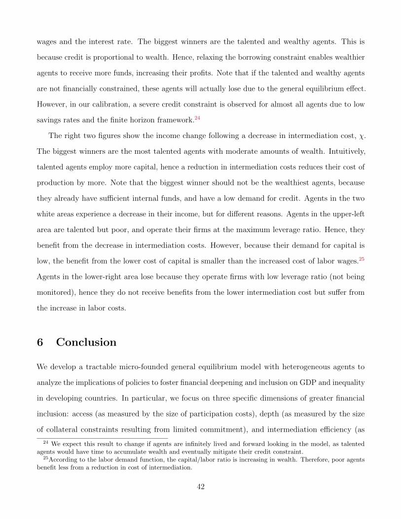
wages and the interest rate. The biggest winners are the talented and wealthy agents. This is

because credit is proportional to wealth. Hence, relaxing the borrowing constraint enables wealthier

agents to receive more funds, increasing their profits. Note that if the talented and wealthy agents

are not financially constrained, these agents will actually lose due to the general equilibrium effect.

However, in our calibration, a severe credit constraint is observed for almost all agents due to low

savings rates and the finite horizon framework.24

The right two figures show the income change following a decrease in intermediation cost, χ.

The biggest winners are the most talented agents with moderate amounts of wealth. Intuitively,

talented agents employ more capital, hence a reduction in intermediation costs reduces their cost of

production by more. Note that the biggest winner should not be the wealthiest agents, because

they already have sufficient internal funds, and have a low demand for credit. Agents in the two

white areas experience a decrease in their income, but for different reasons. Agents in the upper-left

area are talented but poor, and operate their firms at the maximum leverage ratio. Hence, they

benefit from the decrease in intermediation costs. However, because their demand for capital is

low, the benefit from the lower cost of capital is smaller than the increased cost of labor wages.25

Agents in the lower-right area lose because they operate firms with low leverage ratio (not being

monitored), hence they do not receive benefits from the lower intermediation cost but suffer from

the increase in labor costs.

6 Conclusion

We develop a tractable micro-founded general equilibrium model with heterogeneous agents to

analyze the implications of policies to foster financial deepening and inclusion on GDP and inequality

in developing countries. In particular, we focus on three specific dimensions of greater financial

inclusion: access (as measured by the size of participation costs), depth (as measured by the size

of collateral constraints resulting from limited commitment), and intermediation efficiency (as

24 We expect this result to change if agents are infinitely lived and forward looking in the model, as talentedagents would have time to accumulate wealth and eventually mitigate their credit constraint.

25According to the labor demand function, the capital/labor ratio is increasing in wealth. Therefore, poor agentsbenefit less from a reduction in cost of intermediation.

42

measured by the size of the interest rate spread, reflecting default probability and asymmetric

information).

Using analytical and numerical methods, we calibrate the model for six low-income and emerging

market countries (Uganda, Kenya, Mozambique, Malaysia, the Philippines, and Egypt). While our

simulation results are intended to be illustrative, they indicate that relaxing various financial sector

frictions may affect GDP and inequality in different ways.

Importantly, our findings suggest that country-specific characteristics play a central role in

determining the impacts, interactions, and trade-offs between macroeconomic variables and policies.

Thus, understanding the specific constraints generating lack of financial inclusion in an economy

is critical for tailoring policy recommendations. Moreover, the model simulations indicate that

different dimensions of financial inclusion have a differential impact on GDP and inequality and that

there are trade-offs. There also exist rich interactions among the different dimensions of financial

inclusion. Financial sector policies that address these dimensions could be complementary in nature

with each other, but it can also be the case that implementing one policy reduces the effectiveness

of other policies.

What types of financial inclusion policies could be considered? Policies to enhance inclusion

encompass developing appropriate legal, regulatory, and institutional frameworks and supporting

the information environment. The government has a central role to play in enhancing financial

inclusion by introducing laws that protect property and creditor rights and by ensuring that these

laws are adequately enforced. Indeed, country experiences suggest that poorly designed and enforced

creditor rights discourage lending and encourage individuals to default. Improvements in collateral

framework can thus play an important role in alleviating borrowing constraints and reducing

intermediation costs. Indeed, recent evidence suggests that the introduction or reform of registries

for movable collateral (as opposed to fixed assets such as land and buildings), such as machines and

other equipment, can greatly spur firm availability of finance (World Bank, 2014).

Alleviating information asymmetries can reduce credit rationing and have a disciplining effect

on borrowers. The government can enhance financial inclusion by facilitating access to borrower

information or by introducing or reforming credit bureaus and registries. In countries with no

43

private credit bureaus, the establishment of public credit registries can jump start credit reporting,

as long as the registries provide timely and sufficient data on borrowers and their credit worthiness

(e.g., borrowing and repayment behavior to asses default risk). In some countries, buyer-supplier

relationships (e.g., trade credit) can also be another valuable source of credit information. Insolvency

regimes are also a key aspect of financial infrastructure, helping regulate efficient exit from markets

and providing opportunities for recovery by bankrupt entities and their creditors.

Other direct interventions aimed specifically at enhancing banking penetration (e.g., low-fee

accounts, simplified documentation requirement, providing non-financial services to improve record

keeping, improving competition in banking system) can reduce credit participation costs by increasing

access to financial services. Direct interventions in the credit market, such as directed lending

programs and risk-sharing arrangements, can have positive effects on firm access, particularly that

of small and medium enterprises, but country experiences indicate that the design and management

of such schemes can be challenging. Moreover, these concerns are magnified in environments with

weak institutions.

References

Abraham, A. and N. Pavoni (2005, 04/05). The Efficient Allocation of Consumption under

Moral Hazard and Hidden Access to the Credit Market. Journal of the European Economic

Association 3 (2-3), 370–381.

Aghion, P. and P. Bolton (1997, April). A Theory of Trickle-Down Growth and Development.

Review of Economic Studies 64 (2), 151–72.

Albuquerque, R. and H. A. Hopenhayn (2004, 04). Optimal Lending Contracts and Firm Dynamics.

Review of Economic Studies 71 (2), 285–315.

Alem, M. and R. M. Townsend (2013). An Evaluation of Financial Institutions: Impact on

Consumption and Investment Using Panel Data and the Theory of Risk-Bearing. Annals Issue

of the Journal of Econometrics in Honor of Bill Barnett (forthcoming).

44

Amaral, P. S. and E. Quintin (2010, 08). Limited Enforcement, Financial Intermediation, And

Economic Development: A Quantitative Assessment. International Economic Review 51 (3),

785–811.

Andreoni, J. (1989, December). Giving with Impure Altruism: Applications to Charity and

Ricardian Equivalence. Journal of Political Economy 97 (6), 1447–58.

Assuncao, J., S. Mityakov, and R. M. Townsend (2012, September). Ownership Matters: the

Geographical Dynamics of BAAC and CommercialBanks in Thailand. Working paper.

Ayyagari, M., A. Demirgc-Kunt, and V. Maksimovic (2008, July). How Well Do Institutional

Theories Explain Firms’ Perceptions of Property Rights? Review of Financial Studies 21 (4),

1833–1871.

Banerjee, A. V. and E. Duflo (2005, December). Growth Theory through the Lens of Development

Economics. In P. Aghion and S. Durlauf (Eds.), Handbook of Economic Growth, Volume 1 of

Handbook of Economic Growth, Chapter 7, pp. 473–552. Elsevier.

Banerjee, A. V. and A. F. Newman (1993, April). Occupational Choice and the Process of

Development. Journal of Political Economy 101 (2), 274–98.

Banerjee, A. V. and A. F. Newman (2003, November). Inequality, Growth and Trade Policy. Mit

working paper.

Beck, T., A. Demirg-Kunt, and R. Levine (2007, March). Finance, inequality and the poor. Journal

of Economic Growth 12 (1), 27–49.

Beck, T., A. Demirg-Kunt, and V. Maksimovic (2005, 02). Financial and Legal Constraints to

Growth: Does Firm Size Matter? Journal of Finance 60 (1), 137–177.

Buera, F. J., J. P. Kaboski, and Y. Shin (2011, August). Finance and Development: A Tale of Two

Sectors. American Economic Review 101 (5), 1964–2002.

45

Buera, F. J., J. P. Kaboski, and Y. Shin (2012, March). The Macroeconomics of Microfinance.

NBER Working Papers 17905, National Bureau of Economic Research, Inc.

Buera, F. J. and Y. Shin (2013). Financial Frictions and the Persistence of History: A Quantitative

Exploration. Journal of Political Economy 121 (2), 221 – 272.

Burgess, R. and R. Pande (2005, June). Do Rural Banks Matter? Evidence from the Indian Social

Banking Experiment. American Economic Review 95 (3), 780–795.

Cagetti, M. and M. D. Nardi (2006, October). Entrepreneurship, Frictions, and Wealth. Journal of

Political Economy 114 (5), 835–870.

Caselli, F. and N. Gennaioli (2013, 01). Dynastic Management. Economic Inquiry 51 (1), 971–996.

Castaneda, A., J. Diaz-Gimenez, and J.-V. Rios-Rull (2003, August). Accounting for the U.S.

Earnings and Wealth Inequality. Journal of Political Economy 111 (4), 818–857.

Castro, R., G. L. Clementi, and G. Macdonald (2009). Legal Institutions, Sectoral Heterogeneity,

and Economic Development. Review of Economic Studies 76 (2), 529–561.

Clarke, G. R. G., L. C. Xu, and H. fu Zou (2006, January). Finance and Income Inequality: What

Do the Data Tell Us? Southern Economic Journal 72 (3), 578–596.

Clementi, G. L. and H. A. Hopenhayn (2006, 02). A Theory of Financing Constraints and Firm

Dynamics. The Quarterly Journal of Economics 121 (1), 229–265.

Cole, H., J. Greenwood, and J. Sanchez (2012, October). Why Doesn’t Technology Flow from Rich

to Poor Countries? 2012 Meeting Papers 834, Society for Economic Dynamics.

Davies, J. B. (1982, August). The Relative Impact of Inheritance and Other Factors on Economic

Inequality. The Quarterly Journal of Economics 97 (3), 471–98.

D’Erasmo, P. N. and H. J. Moscoso Boedo (2012). Financial structure, informality and development.

Journal of Monetary Economics 59 (3), 286–302.

46

Doepke, M. and R. M. Townsend (2006, January). Dynamic mechanism design with hidden income

and hidden actions. Journal of Economic Theory 126 (1), 235–285.

Evans, D. S. and B. Jovanovic (1989, August). An Estimated Model of Entrepreneurial Choice

under Liquidity Constraints. Journal of Political Economy 97 (4), 808–27.

Gine, X. and R. M. Townsend (2004, August). Evaluation of financial liberalization: a general

equilibrium model with constrained occupation choice. Journal of Development Economics 74 (2),

269–307.

Greenwood, J. and B. Jovanovic (1990, October). Financial Development, Growth, and the

Distribution of Income. Journal of Political Economy 98 (5), 1076–1107.

Greenwood, J., J. Sanchez, and C. Wang (2013, January). Quantifying the Impact of Financial

Development on Economic Development. Review of Economic Dynamics 16 (1), 194–215.

Greenwood, J., J. M. Sanchez, and C. Wang (2010, September). Financing Development: The Role

of Information Costs. American Economic Review 100 (4), 1875–91.

Holtz-Eakin, D., D. Joulfaian, and H. S. Rosen (1994, Summer). Entrepreneurial Decisions and

Liquidity Constraints. RAND Journal of Economics 25 (2), 334–347.

Hsieh, C.-T. and P. J. Klenow (2009, November). Misallocation and Manufacturing TFP in China

and India. The Quarterly Journal of Economics 124 (4), 1403–1448.

Huggett, M. (1996, December). Wealth distribution in life-cycle economies. Journal of Monetary

Economics 38 (3), 469–494.

Jeong, H. and R. Townsend (2007, July). Sources of TFP growth: occupational choice and financial

deepening. Economic Theory 32 (1), 179–221.

Jeong, H. and R. M. Townsend (2008, September). Growth And Inequality: Model Evaluation

Based On An Estimation-Calibration Strategy. Macroeconomic Dynamics 12 (S2), 231–284.

47

Karaivanov, A. and R. M. Townsend (2014, 05). Dynamic Financial Constraints: Distinguishing

Mechanism Design From Exogenously Incomplete Regimes. Econometrica 82 (3), 887–959.

King, R. G. and R. Levine (1993, August). Finance and Growth: Schumpeter Might Be Right. The

Quarterly Journal of Economics 108 (3), 717–37.

Kinnan, C. (2014, January). Distinguishing barriers to insurance in Thai villages. Working Papers

1276, Northwestern University.

Levine, R. (2005, December). Finance and Growth: Theory and Evidence. In P. Aghion and

S. Durlauf (Eds.), Handbook of Economic Growth, Volume 1 of Handbook of Economic Growth,

Chapter 12, pp. 865–934. Elsevier.

Lloyd-Ellis, H. and D. Bernhardt (2000, January). Enterprise, Inequality and Economic Development.

Review of Economic Studies 67 (1), 147–68.

Martin, A. and F. Taddei (2013). International capital flows and credit market imperfections: A

tale of two frictions. Journal of International Economics 89 (2), 441–452.

Midrigan, V. and D. Y. Xu (2014, February). Finance and Misallocation: Evidence from Plant-Level

Data. American Economic Review 104 (2), 422–58.

Moll, B. (2014). Productivity Losses from Financial Frictions: Can Self-Financing Undo Capital

Misallocation? American Economic Review (forthcoming).

Moll, B., R. M. Townsend, and V. Zhorin (2014, March). Economic Development and the Equilibrium

Interaction of Financial Frictions. Working papers.

Nardi, M. D. (2004). Wealth Inequality and Intergenerational Links. Review of Economic Stud-

ies 71 (3), 743–768.

Okuda, H. and F. Mieno (1999, December). What Happened to Thai Commercial Banks in the

Pre-Asian Crisis Period: Microeconomic Analysis of Thai Banking Industry. Hitotsubashi Journal

of Economics 40 (2), 97–121.

48

Paulson, A. L., R. M. Townsend, and A. Karaivanov (2006, February). Distinguishing Limited

Liability from Moral Hazard in a Model of Entrepreneurship. Journal of Political Economy 114 (1),

100–144.

Townsend, R. M. (1979, October). Optimal contracts and competitive markets with costly state

verification. Journal of Economic Theory 21 (2), 265–293.

Townsend, R. M. and K. Ueda (2006). Financial Deepening, Inequality, and Growth: A Model-Based

Quantitative Evaluation. Review of Economic Studies 73 (1), 251–293.

World Bank (2014). Global Financial Development Report: Financial Inclusion. Technical report.

49