I.1.(a) Krylov Subspace Projection Methods
1 Introduction
In this lecture, we discuss iterative methods based on Krylov subspace projection for extractinga few eigenvalues and eigenvectors of a large sparse matrix. Projection techniques are thefoundation of many algorithms. We will first discuss the general framework of the Rayleigh-Ritz subspace projection procedure, and then discuss the widely used Arnoldi and Lanczosmethods.
2 Rayleigh-Ritz procedure
Let A be an n×n complex matrix and K be an m-dimensional subspace of Cn. An orthogonal
projection technique seeks an approximate eigenpair (λ, u), with λ in C and u in K. Thisapproximate eigenpair is obtained by imposing the following Galerkin condition :
Au − λu ⊥ K , (2.1)
or, equivalently,〈Au − λu, v〉 = 0 , ∀ v ∈ K. (2.2)
To translate the condition (2.2) into a matrix problem, assume that an orthonormal basis{v1, v2, . . . , vk} of K is available. Denote V = (v1, v2, . . . , vk), and let u = V y. Then, thecondition (2.2) becomes
〈AV y − λV y, vj〉 = 0, j = 1, . . . , k.
Therefore, y and λ must satisfyBky = λy, (2.3)
whereBk = V HAV.
Each eigenvalue λi of Bk is called a Ritz value, and V yi is called Ritz vector, where yi isthe eigenvector of Bk associated with λi. This procedure A is known as the Rayleigh-Ritz
procedure.
Algorithm 2.1 (Rayleigh-Ritz Procedure).
1. Compute an orthonormal basis {vi}i=1,...,k of the subspace K. Let V = (v1, v2, . . . , vk).
2. Compute Bk = V HAV .
3. Compute the eigenvalues of Bk and select k0 desired ones: λi, i = 1, 2, . . . , k0, wherek0 ≤ k.
4. Compute the eigenvectors yi, i = 1, . . . , k0, of Bk associated with λi, i = 1, . . . , k0, andthe corresponding approximate eigenvectors of A, ui = V yi, i = 1, . . . , k0.
The numerical solution of the small k × k eigenvalue problem in the statements 3 and 4can be treated by standard algorithms for solving small dense eigenvalue problems. Anotherimportant note is that in the statement 4 one can replace eigenvectors by Schur vectors toget approximate Schur vectors ui instead of approximate eigenvectors. Schur vectors can
1
be obtained in a numerically stable way and, in general, eigenvectors are more sensitive torounding errors than are Schur vectors.
Alternatively, there is an oblique projection technique. Here we first select two subspacesL and K and then seek an approximation u ∈ K and an element λ ∈ C that satisfy thePetrov-Galerkin condition :
〈Au − λu, v〉 = 0, ∀ v ∈ L . (2.4)
The subspace K will be referred to as the right subspace and L as the left subspace. Aprocedure similar to the Rayleigh-Ritz procedure can be devised. Let V denote the basis forthe subspace K and W for L. Then, writing u = V y, the Petrov-Galerkin condition (2.4) yieldsthe reduced eigenvalue problem
Bky = λCky,
whereBk = WHAV and Ck = WHV.
If Ck = I, then the two bases are called biorthonormal. In order for a biorthonormal pair Vand W to exist the following additional assumption for L and K must hold. For any two basesV and W of K and L, respectively,
det(WHV ) 6= 0 . (2.5)
As can be seen this condition does not depend on the bases selected and is equivalent torequiring that no vector of K is orthogonal to L.
3 Optimality
We now examine the Rayleigh-Ritz procedure in further detail. Let Q = (Qk, Qu) be an n-by-northogonal matrix, where Qk is n-by-k, and Qu is n-by-(n − k), and span(Qk) = K. Then
T = QT AQ = (Qk, Qu)T A(Qk, Qu) =
(QT
k AQk QTk AQu
QTu AQk QT
u AQu
)≡(
Tk Tuk
Tku Tu
)
The Ritz values and Ritz vectors are considered optimal approximations to the eigenvaluesand eigenvectors of A from the selected subsapce K = span(Qk) as justified by the followingtheorem.
Theorem 3.1. The minimum of ‖AQk − QkS‖2 over all k-by-k S is attained by S = Tk, inwhich case, ‖AQk − QkTk‖2 = ‖Tku‖2.
Proof. Let S = Tk + Z. We will show that ‖AQk − QkS‖2 is minimized when Z = 0. This isa consequence of
(AQk − QkS)T (AQk − QkS)
= [AQk − Qk(Tk + Z)]T [AQk − Qk(Tk + Z)]
= (AQk − QkTk)T (AQk − QkTk) − (AQk − QkTk)
T (QkZ)
− (QkZ)T (AQk − QkTk) + (QkZ)T (QkZ)
= (AQk − QkTk)T (AQk − QkTk) − (QT
k AT Qk − T Tk )Z
− ZT (QTk AQk − Tk) + ZT Z
= (AQk − QkTk)T (AQk − QkTk) + ZT Z. (3.6)
2
Furthermore, it is easy to compute the minimum value
‖AQk − QkTk‖2 = ‖(QkTk + QuTku) − QkTk‖2 = ‖QuTku‖2 = ‖Tku‖2,
as expected.
More can be said from the identity (3.6): The conclusion of Theorem 3.1 remains valid ifthe spectral norm ‖ · ‖2 is replaced by any unitarily invariant norm, including in particular theFrobenius norm.
Corollary 3.1. Let A be a symmetric matrix, AT = A, and let Tk = V ΛV T be the eigen-decomposition of Tk. The minimum of ‖APk − PkD‖ over all n-by-k orthogonal matrices Pk
subject to span(Pk) = span(Qk) and over all diagonal D is also ‖Tku‖2 and is attained byPk = QkV and D = Λ.
Proof. If we replace Qk with QkU in the above proof, where U is another orthogonal matrix,then the columns of Qk and QkU span the same space, and
‖AQk − QkS‖2 = ‖AQkU − QkSU‖2 = ‖A(QkU) − (QkU)(UT SU)‖2.
These quantities are still minimized when S = Tk, and by choosing U = V so that UT TkU isdiagonal.
4 Krylov subspace
As we know, the simplest thing to do is to compute just the largest eigenvalue in absolutevalue, along with its eigenvector. The power method is the simplest algorithm suitable for thistask. Starting with a given u0, k iterations of the power method produce a sequence of vectorsu0, u1, u2, . . . , uk. It is easy to see that these vectors span a Krylov Subspace :
Kk+1(A, u0) = span{u0, u1, u2, . . . , uk} = span{u0, Au0, A2u0, . . . , A
ku0}.
Now, rather than taking uk as our approximate eigenvector, it is natural to ask for the “best”approximate eigenvector in Kk+1(A, u0). We will see that the best eigenvector (and eigenvalue)approximations from Kk+1(A, u0) are much better than uk alone.
Charaterization of Kk+1(A, u0):
Kk+1(A, u0) = {q(A)u0 | q ∈ Pk},
where Pk is the set of all polynomial of degree less than k + 1.
Properties of Kk+1(A, u0):
1. Kk(A, u0) ⊂ Kk+1(A, u0).
AKk(A, u0) ⊂ Kk+1(A, u0).
2. If σ 6= 0, Kk(A, u0) = Kk(σA, u0) = Kk(A, σu0).
3. For any κ, Kk(A, u0) = Kk(A − κI, u0).
4. If W is nonsingular, Kk(W−1AW, W−1u0) = W−1Kk(A, u0).
An explicit Krylov basis {u0, Au0, A2u0, . . . , A
ku0} is not suitable for numerical computing.It is extremely ill-conditioned. Therefore, our first task is to replace a Krylov basis with a betterconditioned basis, say an orthonormal basis.
3

Theorem 4.1. Let the columns of Kj+1 =(u0 Au0 . . . Aju0
)be linearly independent. Let
Kj+1 = Uj+1Rj+1 (4.7)
be the QR factorization of Kj+1. Then there is a (j+1)×j unreduced upper Hessenberg matrix
Hj such that
AUj = Uj+1Hj . (4.8)
Conversely, if Uj+1 is orthonormal and satisfies (4.8), then
span(Uj+1) = span{u0, Au0, . . . , Aju0}. (4.9)
Proof. Partitioning the QR decomposition (4.7), we have
(Kj Aju0
)=(Uj uj+1
)(Rj rj+1
0 rj+1,j+1
),
where Kj = UjRj is the QR decomposition of Kj . Then
AKj = AUjRj
or
AUj = AKjR−1j = Kj+1
(0
R−1j
)= Uj+1Rj+1
(0
R−1j
).
It is easy to verify that
Hj = Rj+1
(0
R−1j
)
is a (j +1)× j unreduced upper Hessenberg matrix. Therefore we complete the proof of (4.8).Conversely, suppose that Uj+1 satisfies (4.8), then by induction, we can prove the identity
(4.9).
We note that by partitioning,
Hj =
(Hj
hj+1,jeTj
),
the decomposition (4.8) can be written in the following form that will be useful in the sequel:
AUj = UjHj + hj+1,juj+1eTj . (4.10)
We call (4.10) an Arnoldi decomposition of order j. The decomposition (4.8) is acompact form.
5 Arnoldi algorithm
The Arnoldi algorithm for finding a few eigenpairs of a general matrix A combines the Arnoldiprocess for building a Krylov subspace with the Raleigh-Ritz procedure.
First, by the Arnoldi decomposition (4.10), we deduce the following process to generate anorthogonormal basis {v1, v2, . . . , vm} of the Krylov subspace Km(A, v):
4
Algorithm 5.1 (Arnoldi Process).1. v1 = v/‖v‖2
2. for j = 1, 2, . . . , k3. compute w = Avj
4. for i = 1, 2, . . . , j5. hij = vT
i w6. w = w − hijvi
7. end for8. hj+1,j = ‖w‖2
9. If hj+1,j = 0, stop10. vj+1 = wj/hj+1,j
11. endfor
Remark 5.1. (1) Note that the matrix A is only referenced via the matrix-vector multi-plication Avj . Therefore, it is ideal for large sparse or large dense structured matrices. Anysparsity or structure of a matrix can be exploited in the matrix-vector multiplication. (2)The main storage requirement is (m + 1)n for storing Arnoldi vectors {vi} plus the storagerequirement for the matrix A in question or the required matrix-vector multiplication. (3) Theprimary arithmetic cost of the procedure is the cost of m matrix-vector products plus 2m2nfor the rest. It is common that the matrix-vector multiplication is the dominant cost. (4) TheArnoldi procedure breaks down when hj+1,j = 0 for some j. It is easy to see that if the Arnoldiprocedure breaks down at step j (i.e. hj+1,j = 0), then Kj = span(Vj) is invariant subspace ofA. (5) Some care must be taken to insure that the vectors vj remain orthogonal to workingaccuracy in the presence of rounding error. The usual technique is reorthogonalization.
DenoteVk =
(v1 v2 . . . vk
)
and
Hk =
h11 h12 · · · h1,k−1 h1k
h21 h22 · · · h2,k−1 h2k
h32. . . h3,k−1 h3k
. . ....
...hk,k−1 hkk
.
In the matrix form, the Arnoldi process can be expressed in the following governing relations:
AVk = VkHk + hk+1,kvk+1eTk (5.11)
andV H
k Vk = I and V Hk vk+1 = 0.
Note that the decomposition is uniquely determined by the starting vector v. This is commonlyknown as the implicit Q-Theorem.
Since V Hk vk+1 = 0, we have
Hk = V Tk AVk.
Thus, Hk is called the generalized Rayleigh Quotient Matrix corresponding to Vk. Let µbe an eigenvalue of Hk and y be a corresponding eigenvector y, i.e.,
Hky = µy, ‖y‖2 = 1.
Then the corresponding Ritz pair is (µ, Vky). Applying y to the right hand side of (5.11), theresidual vector for (µ, Vky) is given by
A(Vky) − µ(Vky) = hk+1,kvk+1(eTk y).
5
Using the backward error interpretation, we know that (µ, Vky) is an exact eigenpair of A+E,where ‖E‖2 = |hk+1,k| · |eT
k y|. This gives us a criterion of whether to accept the Ritz pair(µ, Vky) as an accurate approximate eigenpair of A.1
An outline of Arnoldi’s method for the nonsymmetric eigenvalue problem is as follows.
Algorithm 5.2 (Arnoldi algorithm).
1. Choose a starting vector v;
2. Generate the Arnoldi decomposition of length k by the Arnoldi process;
3. Compute the Ritz pairs and decide which ones are acceptable;
4. If necessary, increase k and repeat.
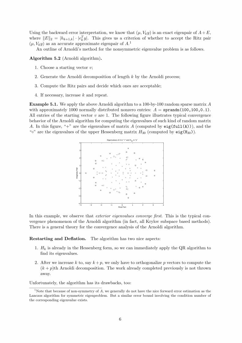
Example 5.1. We apply the above Arnoldi algorithm to a 100-by-100 random sparse matrix Awith approximately 1000 normally distributed nonzero entries: A = sprandn(100,100,0.1).All entries of the starting vector v are 1. The following figure illustrates typical convergencebehavior of the Arnoldi algorithm for computing the eigenvalues of such kind of random matrixA. In this figure, “+” are the eigenvalues of matrix A (computed by eig(full(A))), and the“◦” are the eigenvalues of the upper Hessenberg matrix H30 (computed by eig(H30)).
−4 −3 −2 −1 0 1 2 3 4−4
−3
−2
−1
0
1
2
3
4
Real Part
Imag
inar
y P
art
Eigenvalues of A in "+" and H30
in "o"
In this example, we observe that exterior eigenvalues converge first. This is the typical con-vergence phenomenon of the Arnoldi algorithm (in fact, all Krylov subspace based methods).There is a general theory for the convergence analysis of the Arnoldi algorithm.
Restarting and Deflation. The algorithm has two nice aspects:
1. Hk is already in the Hessenberg form, so we can immediately apply the QR algorithm tofind its eigenvalues.
2. After we increase k to, say k +p, we only have to orthogonalize p vectors to compute the(k + p)th Arnoldi decomposition. The work already completed previously is not thrownaway.
Unfortunately, the algorithm has its drawbacks, too:
1Note that because of non-symmetry of A, we generally do not have the nice forward error estimation as theLanczos algorithm for symmetric eigenproblem. But a similar error bound involving the condition number ofthe corresponding eigenvalue exists.
6

1. If A is large, we cannot increase k indefinitely, since Vk requires nk memory locations tostore.
2. We have little control over which eigenpairs the algorithm finds. In a given applicationwe will be interested in a certain set of eigenpairs. For example, eigenvalues lying nearthe imaginary axis. There is nothing in the algorithm to force desired eigenvectors intothe subspace or the discard undesired ones.
We will now show how to implicitly restart the algorithm with a new Arnoldi decompositionin which (in exact arithmetic) the unwanted eigenvalues have been purged from Hk.
Implicit Restarting. We begin by asking how to cast an undesired eigenvalue out of anunreduced Hessenberg matrix H. Let µ be the eigenvalue of H, and suppose we perform onestep of the QR algorithm with shift µ. The first step is to determine an orthogonal matrix Usuch that
R = UH(H − µI)
is upper triangular. Since H−µI is singular, R must have a zero on its diagonal. Because H isunreduced, that zero cannot occur at a diagonal position other than the last, namely rnn = 0.and the last row of R is zero.
Furthermore, note that U = P12P23 · · ·Pn−1,n, where Pi,i+1 is a rotation in the (i, i + 1)-plane. Consequently, U is Hessenberg and can be partitioned in the form
U =
(U∗ u
uk,k−1eTk−1 uk,k
).
Hence
H ′ = RU + µI =
(H∗ h0 µ
)= UHHU.
In other words, the shifted QR step has found the eigenvalue µ exactly and has deflated theproblem.
In the presence of rounding error we cannot expect the last element of R to be zero. Thismeans that the matrix H will have the form
H ′ = UHHU =
(H∗ h
hk,k−1eTk−1 µ
).
We are now going to show how to use the transformation U to reduce the size of the Arnoldidecomposition.
By the relation (5.11), we have
AVkU = VkU(UT HkU) + hk+1,kvk+1eTk U .
If we partition
Vk = VkU =(Vk−1 vk
)
Then
A ( Vk−1 vk ) = ( Vk−1 vk )
(H∗ h
hk,k−1eTk−1 µ
)+ hk+1,kvk+1
(uk,k−1e
Tk−1 uk,k
).
Computing the first k − 1 columns of this partition, we get
AVk−1 = Vk−1H∗ + feTk−1, (5.12)
7
where f = hk,k−1vk + hk+1,kuk,k−1vk+1.
The matrix H∗ is Hessenberg. The vector f is orthogonal to the columns of Vk−1. Hence(5.12) is an Arnoldi decomposition of length k − 1. With exact computation, the eigenvalue µis not presented in H∗.
The process may be repeated to remove other unwanted values from H. If the matrix is real,a pair of complex conjugate eigenvalues can be removed at the same time via an implicit doubleshift. The key observation here is that V is zero below its second subdiagonal element, so thattruncating the last two columns and adjusting the residual results in an Arnoldi decompositioncan be done together. Once un-desired eigenvalues have been removed from H, the Arnoldidecomposition may be expanded again and the process repeats.
Deflation. There are two important additions to the algorithm that are beyond the scopeof this lecture.
1. First, as Ritz pairs converge they can be locked into the decomposition. The procedureamounts to computing an Arnoldi decomposition of the form
A ( V1 V2 ) = ( V1 V2 )
(H11 H12
0 H22
)+ hk+1,kvk+1e
Tk
When this is done, one can work with the part of decomposition corresponding to V2, thussaving multiplications by A. (However, care must be taken to maintain orthogonality tothe columns of V1.)
2. The second addition concerns unwanted Ritz pairs. The restarting procedure will tendto purge the unwanted eigenvalues from H. But the columns of U may have significantcomponents along the eigenvectors corresponding to the purged pairs, which will thenreappear as the decomposition is expanded. If certain pair are too persistent, it is bestto keep them around by computing a block diagonal decomposition of the form
A ( V1 V2 ) = ( V1 V2 )
(H11 00 H22
)+ ηvk+1e
Tk ,
where H11 contains the unwanted eigenvalues. This insures that U2 has negligible compo-nents along the unwanted eigenvectors. We can then compute an Arnoldi decompositionby reorthognalizing the relation
AV2 = H22V2 + ηvk+1eTm,
where m is the order of H2.
6 The symmetric Lanczos algorithm
The Lanczos algorithm for finding a few eigenpairs of a symmetric matrix A combines theLanczos process for building a Krylov subspace with the Raleigh-Ritz procedure.
Let us begin with an observation that in the Arnoldi decomposition (4.10), if A is symmet-ric, then the upper Hessenberg matrix Hj is symmetric tridiagonal. Therefore, we have thefollowing simplified process to compute an orthonormal basis of a Krylov subspace:
Algorithm 6.1 (Lanczos process).1 q1 = v/‖v‖2, β0 = 0; q0 = 0;2 for j = 1 to k, do3 w = Aqj ;
8
4 αj = qTj w;
5 w = w − αjqj − βj−1qj−1;6 βj = ‖w‖2;7 if βj = 0, quit;8 qj+1 = w/βj ;9 EndDo
DenoteQk =
(q1 q2 . . . qk
)
and
Tk =
α1 β1
β1 α2 β2
. . .. . .
. . .. . . αk−1 βk−1
βk−1 αk
= tridiag(βj , αj , βj+1),
the k-step Lanczos process yields a fundamental relation
AQk = QkTk + fkeTk , fk = βkqk+1 (6.13)
and QTk Qk = I and QT
k qk+1 = 0.Let µ be an eigenvalue of Tk and y be a corresponding eigenvector y, i.e.,
Tky = µy, ‖y‖2 = 1.
Apply y to the right of (6.13) to get
A(Qky) = QkTky + fk(eTk y) = µ(Qky) + fk(e
Tk y). (6.14)
Here µ is a Ritz value, and Qky is the corresponding Ritz vector . Equation (6.14) offers aquick insight into convergence of the Ritz value and vector.
If fk(eTk y) = 0 for some k, then the associated Ritz value µ is an eigenvalue of A with the
corresponding eigenvector Qky. In general, it is unlikely that fk(eTk y) = 0, but we hope that
the residual norm ‖fk(eTk y)‖2 may be small; and when this happens we expect that µ is going
to be a good approximate to A’s eigenvalue. Indeed, we have the following result.
Lemma 6.1. Let H be (real) symmetric, and Hz − µz = r and z 6= 0. Then
minλ∈eig(H)
|λ − µ| ≤ ‖r‖2/‖z‖2.
Proof. Let H = UΛUT be the eigen-decomposition of H. Then
(H − µI)z = r ⇒ U(Λ − µI)UT z = r ⇒ (Λ − µI)(UT z) = UT r.
Notice that Λ − µI is diagonal. Thus
‖r‖2 = ‖UT r‖2 = ‖(Λ − µI)(UT z)‖2 ≥ minλ∈eig(H)
|λ − µ| ‖UT z‖2 = minλ∈eig(H)
|λ − µ|‖z‖2,
as expected.
The following corollary is a consequence of above Lemma 6.1.
9
Corollary 6.1. There is an eigenvalue λ of A such that
|λ − µ| ≤ ‖fk(eTk y)‖2
‖Qky‖2=
|βk| · |eTk y|
‖Qky‖2.
In the absence of roundoff error, ‖Qky‖2 = ‖y‖2 = 1, and thus the denominator ‖Qky‖2 canbe dropped . But numerically the loss of orthogonality in the columns of Qk can destroy thisidentity. This loss of orthogonality motivated the developments of various reorthogonalizationstrategies.
In summary, we have the following Lanczos algorithm in the simplest form.
Algorithm 6.2 (Simple Lanczos Algorithm).1. q1 = v/‖v‖2, β0 = 0, q0 = 0;2. for j = 1 to k do3. w = Aqj ;4. αj = qT
j w;
5. w = w − αjqj − βj−1qj−1;6. βj = ‖w‖2;7. if βj = 0, quit;8. qj+1 = w/βj ;9. Compute eigenvalues and eigenvectors of Tj
10. Test for convergence11. EndDo
Caveat. All the discussion so far is under the assumption of exact arithmetic. In the pres-ence of finite precision arithmetic, the numerical behaviors of the Lanczos algorithm couldbe significantly different. For example, in finite precision arithmetic, the orthogonality of thecomputed Lanczos vectors {qj} is lost when j is as small as 10 or 20. The simplest remedy(and also the most expensive one) is to implement the the full reorthogonalization, namelyafter the step 5, do
w = w −j−1∑
i=1
(wT qi)qi.
This is called the Lanczos algorithm with full reorthogonalization. (Sometimes, it may beneeded to execute twice). A more elaborate scheme, necessary when convergence is slow andseveral eigenvalues are sought, is to use the selective orthogonalization.
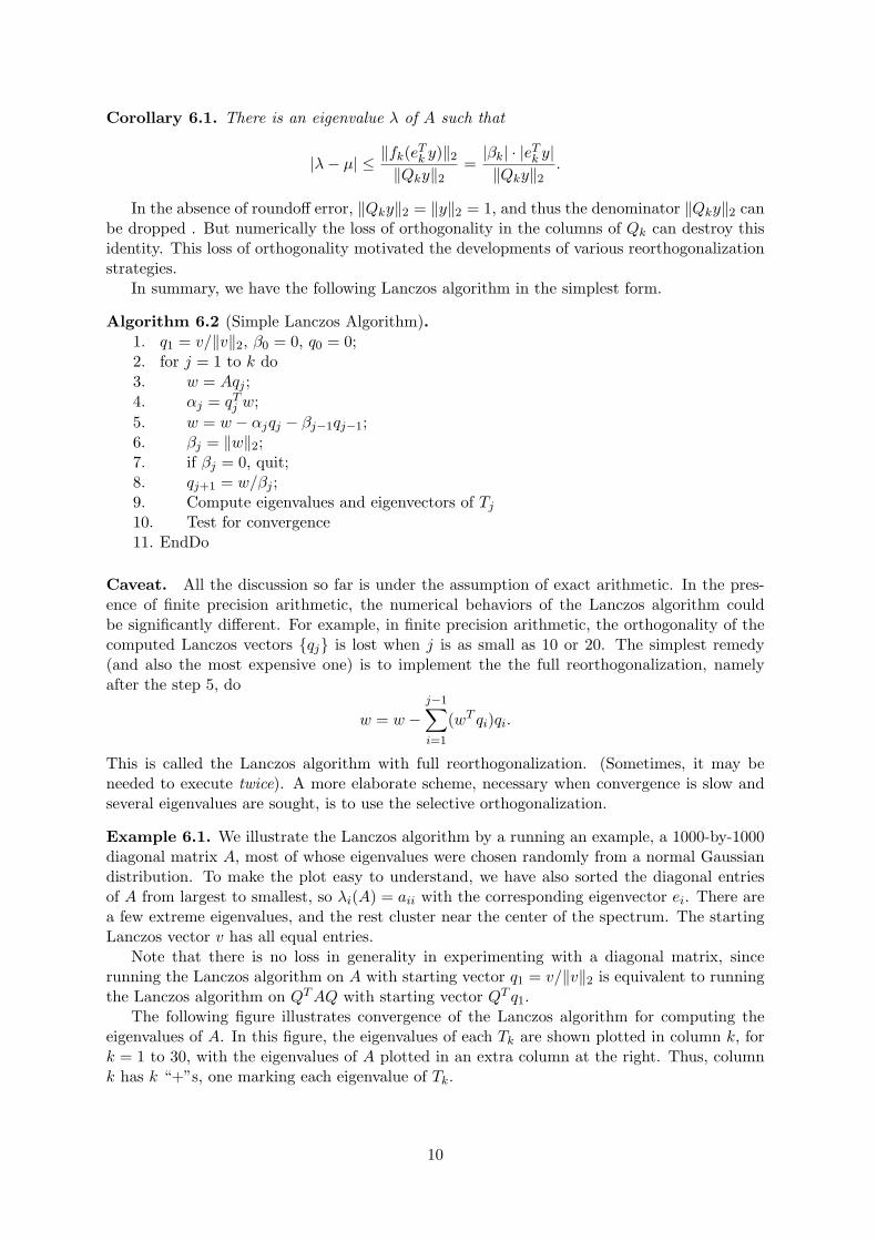
Example 6.1. We illustrate the Lanczos algorithm by a running an example, a 1000-by-1000diagonal matrix A, most of whose eigenvalues were chosen randomly from a normal Gaussiandistribution. To make the plot easy to understand, we have also sorted the diagonal entriesof A from largest to smallest, so λi(A) = aii with the corresponding eigenvector ei. There area few extreme eigenvalues, and the rest cluster near the center of the spectrum. The startingLanczos vector v has all equal entries.
Note that there is no loss in generality in experimenting with a diagonal matrix, sincerunning the Lanczos algorithm on A with starting vector q1 = v/‖v‖2 is equivalent to runningthe Lanczos algorithm on QT AQ with starting vector QT q1.
The following figure illustrates convergence of the Lanczos algorithm for computing theeigenvalues of A. In this figure, the eigenvalues of each Tk are shown plotted in column k, fork = 1 to 30, with the eigenvalues of A plotted in an extra column at the right. Thus, columnk has k “+”s, one marking each eigenvalue of Tk.
10
0 5 10 15 20 25 30
−3
−2
−1
0
1
2
3
30 steps of Lanczos (full reorthogonalization) applied to A
Lanczos step
Eig
enva
lues
To understand convergence, consider the largest eigenvalues of each Tk, note that they in-crease monotonically as k increases; this is a consequence of the Cauchy interlace theorem. Acompletely analogous phenomenon occurs with the smallest eigenvalues.
Now we can ask to which eigenvalue of A the eigenvalue λi(Tk) converges as k increases.Clearly, the largest eigenvalue of Tk, λ1(Tk), ought to converge to the largest eigenvalue ofA, λ1(A). Similarly, the ith largest eigenvalue λi(Tk) of Tk must increase monotonically andconverge to the ith largest eigenvalue λi(A) of A.
In summarizing the discussion, we observe that
1. Extreme eigenvalues, i.e., the largest and smallest ones, converge first, and the interioreigenvalues converge last.
2. Convergence is monotonic, with the ith largest (smallest) eigenvalues of Tk increasing(decreasing) to the ith laregst (smallest) eigenvalue of A, provided that the Lanczosalgorithm does not stop prematurely with some βk = 0.
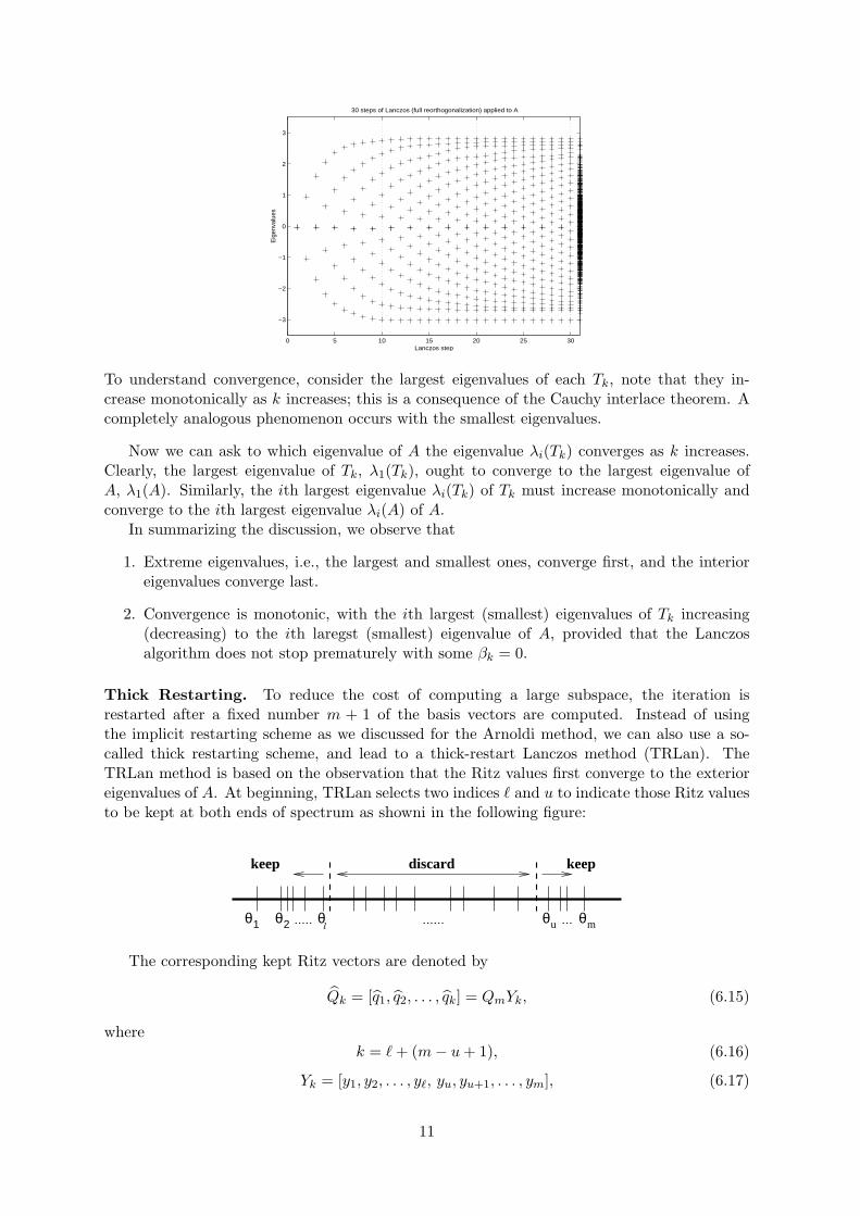
Thick Restarting. To reduce the cost of computing a large subspace, the iteration isrestarted after a fixed number m + 1 of the basis vectors are computed. Instead of usingthe implicit restarting scheme as we discussed for the Arnoldi method, we can also use a so-called thick restarting scheme, and lead to a thick-restart Lanczos method (TRLan). TheTRLan method is based on the observation that the Ritz values first converge to the exterioreigenvalues of A. At beginning, TRLan selects two indices ℓ and u to indicate those Ritz valuesto be kept at both ends of spectrum as showni in the following figure:
θmθ2θ1 θuθ
keep keepdiscard
l
The corresponding kept Ritz vectors are denoted by
Qk = [q1, q2, . . . , qk] = QmYk, (6.15)
wherek = ℓ + (m − u + 1), (6.16)
Yk = [y1, y2, . . . , yℓ, yu, yu+1, . . . , ym], (6.17)
11
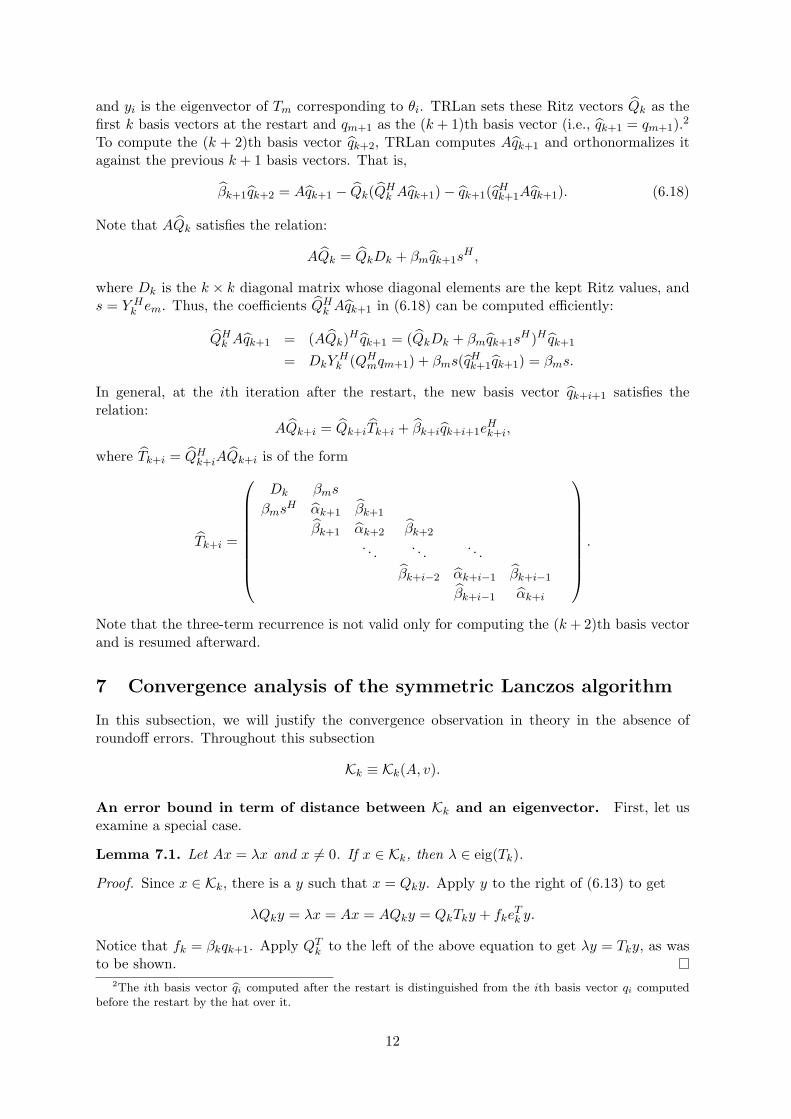
and yi is the eigenvector of Tm corresponding to θi. TRLan sets these Ritz vectors Qk as thefirst k basis vectors at the restart and qm+1 as the (k + 1)th basis vector (i.e., qk+1 = qm+1).
2
To compute the (k + 2)th basis vector qk+2, TRLan computes Aqk+1 and orthonormalizes itagainst the previous k + 1 basis vectors. That is,
βk+1qk+2 = Aqk+1 − Qk(QHk Aqk+1) − qk+1(q
Hk+1Aqk+1). (6.18)
Note that AQk satisfies the relation:
AQk = QkDk + βmqk+1sH ,
where Dk is the k × k diagonal matrix whose diagonal elements are the kept Ritz values, ands = Y H
k em. Thus, the coefficients QHk Aqk+1 in (6.18) can be computed efficiently:
QHk Aqk+1 = (AQk)
H qk+1 = (QkDk + βmqk+1sH)H qk+1
= DkYHk (QH
mqm+1) + βms(qHk+1qk+1) = βms.
In general, at the ith iteration after the restart, the new basis vector qk+i+1 satisfies therelation:
AQk+i = Qk+iTk+i + βk+iqk+i+1eHk+i,
where Tk+i = QHk+iAQk+i is of the form
Tk+i =
Dk βms
βmsH αk+1 βk+1
βk+1 αk+2 βk+2
. . .. . .
. . .
βk+i−2 αk+i−1 βk+i−1
βk+i−1 αk+i
.
Note that the three-term recurrence is not valid only for computing the (k + 2)th basis vectorand is resumed afterward.
7 Convergence analysis of the symmetric Lanczos algorithm
In this subsection, we will justify the convergence observation in theory in the absence ofroundoff errors. Throughout this subsection
Kk ≡ Kk(A, v).
An error bound in term of distance between Kk and an eigenvector. First, let usexamine a special case.
Lemma 7.1. Let Ax = λx and x 6= 0. If x ∈ Kk, then λ ∈ eig(Tk).
Proof. Since x ∈ Kk, there is a y such that x = Qky. Apply y to the right of (6.13) to get
λQky = λx = Ax = AQky = QkTky + fkeTk y.
Notice that fk = βkqk+1. Apply QTk to the left of the above equation to get λy = Tky, as was
to be shown.2The ith basis vector bqi computed after the restart is distinguished from the ith basis vector qi computed
before the restart by the hat over it.
12
In general, if an eigenvector x of A is nearly in the Krylov subspace Kk, we would expectthe corresponding eigenvalue be well approximated by the process.
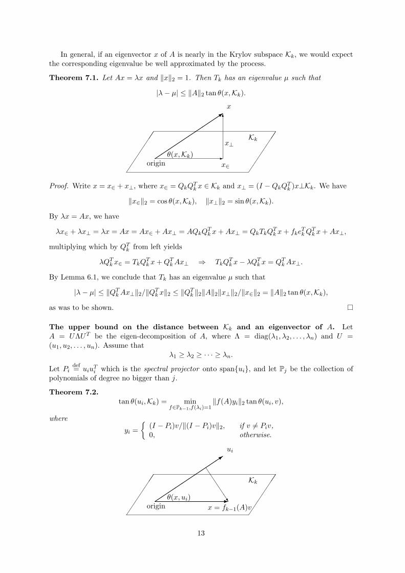
Theorem 7.1. Let Ax = λx and ‖x‖2 = 1. Then Tk has an eigenvalue µ such that
|λ − µ| ≤ ‖A‖2 tan θ(x,Kk).
��
��
��
��
��3
-
6
originθ(x,Kk)
x∈
x⊥
x
Kk
Proof. Write x = x∈ + x⊥, where x∈ = QkQTk x ∈ Kk and x⊥ = (I − QkQ
Tk )x⊥Kk. We have
‖x∈‖2 = cos θ(x,Kk), ‖x⊥‖2 = sin θ(x,Kk).
By λx = Ax, we have
λx∈ + λx⊥ = λx = Ax = Ax∈ + Ax⊥ = AQkQTk x + Ax⊥ = QkTkQ
Tk x + fke
Tk QT
k x + Ax⊥,
multiplying which by QTk from left yields
λQTk x∈ = TkQ
Tk x + QT
k Ax⊥ ⇒ TkQTk x − λQT
k x = QTk Ax⊥.
By Lemma 6.1, we conclude that Tk has an eigenvalue µ such that
|λ − µ| ≤ ‖QTk Ax⊥‖2/‖QT
k x‖2 ≤ ‖QTk ‖2‖A‖2‖x⊥‖2/‖x∈‖2 = ‖A‖2 tan θ(x,Kk),
as was to be shown.
The upper bound on the distance between Kk and an eigenvector of A. LetA = UΛUT be the eigen-decomposition of A, where Λ = diag(λ1, λ2, . . . , λn) and U =(u1, u2, . . . , un). Assume that
λ1 ≥ λ2 ≥ · · · ≥ λn.
Let Pidef= uiu
Ti which is the spectral projector onto span{ui}, and let Pj be the collection of
polynomials of degree no bigger than j.
Theorem 7.2.
tan θ(ui,Kk) = minf∈Pk−1,f(λi)=1
‖f(A)yi‖2 tan θ(ui, v),
where
yi =
{(I − Pi)v/‖(I − Pi)v‖2, if v 6= Piv,0, otherwise.
��
��
��
��
��3
-
JJ
JJJ
originθ(x, ui)
x = fk−1(A)v
ui
Kk
13
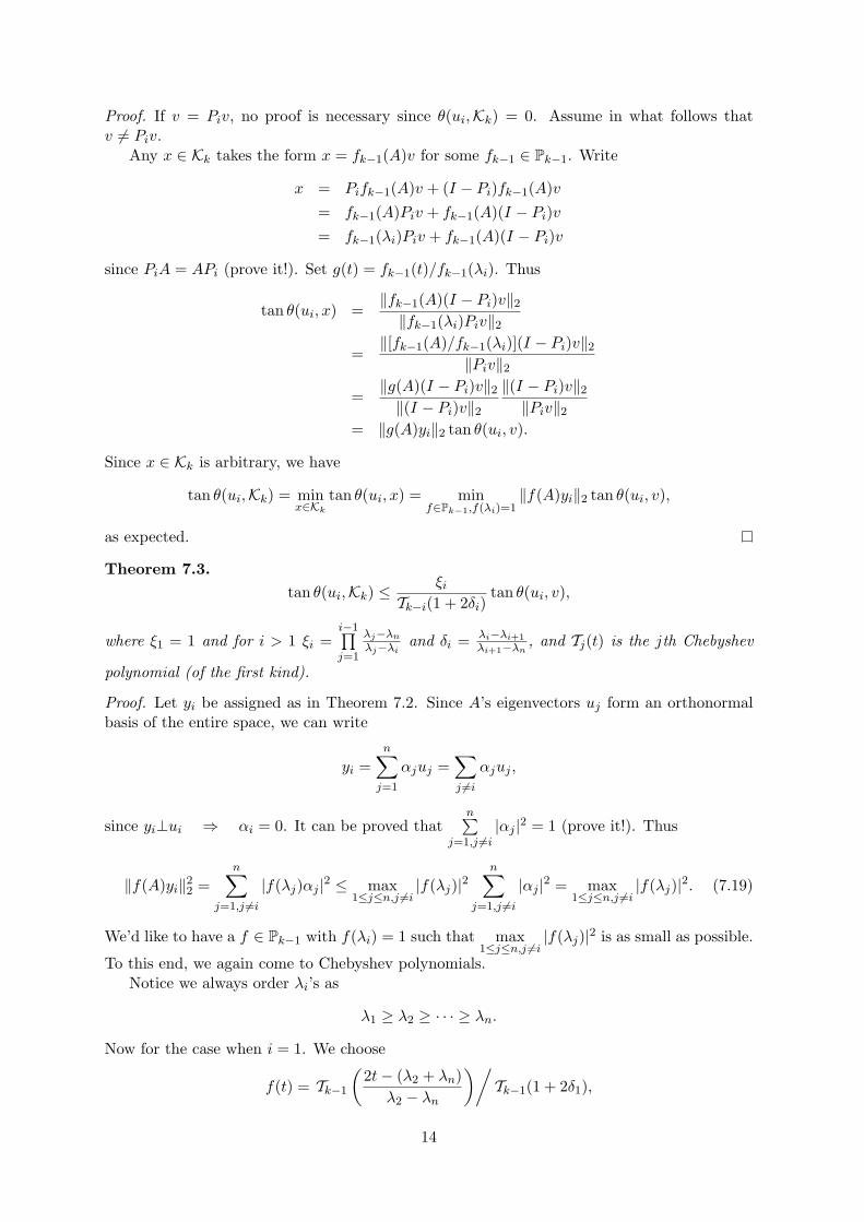
Proof. If v = Piv, no proof is necessary since θ(ui,Kk) = 0. Assume in what follows thatv 6= Piv.
Any x ∈ Kk takes the form x = fk−1(A)v for some fk−1 ∈ Pk−1. Write
x = Pifk−1(A)v + (I − Pi)fk−1(A)v
= fk−1(A)Piv + fk−1(A)(I − Pi)v
= fk−1(λi)Piv + fk−1(A)(I − Pi)v
since PiA = APi (prove it!). Set g(t) = fk−1(t)/fk−1(λi). Thus
tan θ(ui, x) =‖fk−1(A)(I − Pi)v‖2
‖fk−1(λi)Piv‖2
=‖[fk−1(A)/fk−1(λi)](I − Pi)v‖2
‖Piv‖2
=‖g(A)(I − Pi)v‖2
‖(I − Pi)v‖2
‖(I − Pi)v‖2
‖Piv‖2
= ‖g(A)yi‖2 tan θ(ui, v).
Since x ∈ Kk is arbitrary, we have
tan θ(ui,Kk) = minx∈Kk
tan θ(ui, x) = minf∈Pk−1,f(λi)=1
‖f(A)yi‖2 tan θ(ui, v),
as expected.
Theorem 7.3.
tan θ(ui,Kk) ≤ξi
Tk−i(1 + 2δi)tan θ(ui, v),
where ξ1 = 1 and for i > 1 ξi =i−1∏j=1
λj−λn
λj−λiand δi = λi−λi+1
λi+1−λn, and Tj(t) is the jth Chebyshev
polynomial (of the first kind).
Proof. Let yi be assigned as in Theorem 7.2. Since A’s eigenvectors uj form an orthonormalbasis of the entire space, we can write
yi =n∑
j=1
αjuj =∑
j 6=i
αjuj ,
since yi⊥ui ⇒ αi = 0. It can be proved thatn∑
j=1,j 6=i
|αj |2 = 1 (prove it!). Thus
‖f(A)yi‖22 =
n∑
j=1,j 6=i
|f(λj)αj |2 ≤ max1≤j≤n,j 6=i
|f(λj)|2n∑
j=1,j 6=i
|αj |2 = max1≤j≤n,j 6=i
|f(λj)|2. (7.19)
We’d like to have a f ∈ Pk−1 with f(λi) = 1 such that max1≤j≤n,j 6=i
|f(λj)|2 is as small as possible.
To this end, we again come to Chebyshev polynomials.Notice we always order λi’s as
λ1 ≥ λ2 ≥ · · · ≥ λn.
Now for the case when i = 1. We choose
f(t) = Tk−1
(2t − (λ2 + λn)
λ2 − λn
)/Tk−1(1 + 2δ1),
14

for which max2≤j≤n
|f(λj)|2 ≤ 1/Tk−1(1 + 2δ1) and f(λ1) = 1. This, together with Theorem 7.2,
conclude the proof.In general for i > 1, we shall consider polynomials of form
f(t) =(λ1 − t) · · · (λi−1 − t)
(λ1 − λi) · · · (λi−1 − λi)g(t), (7.20)
and search a g ∈ Pk−i such that maxi+1≤j≤n
|g(λj)|2 is as small as possible and g(λi) = 1. To this
end, we choose
g(t) = Tk−i
(2t − (λi+1 + λn)
λi+1 − λn
)/Tk−i(1 + 2δi),
for which max1≤j≤n,j 6=i
|g(λj)|2 ≤ 1/Tk−i(1 + 2δi) and g(λi) = 1. This, together with Theorem 7.2
and (7.19) and (7.20), conclude the proof.
The bounds in Theorem 7.3 turn to get more and more complicated as the index i gets biggerand bigger. Especially it yields nothing about approximating the last eigenvector un. This isin fact due to the way the theorem is derived, not the intrinsic property of Krylov subspaceapproximations; as a matter of fact, the Krylov subspaces favor equally well to eigenspacescorresponding to both ends of eigenvalues. This can be seen by applying Theorem 7.3 to −A,noticing that
Kk(A, v) = Kk(−A, v).
Error bounds of the Lanczos algorithm – Kaniel and Saad Theorems. We mayexclude the case when some βi = 0 in the Lanczos Process and then an invariant subspace ofA is found.
Notice that we have q1 = v/‖v‖2 and
AQk = QkTk + fkeTk = QkTk + βkqk+1e
Tk .
Lemma 7.2. qT1 Aiqk+1 = 0 = qT
1 Aifk for i < k. Thus qT1 f(A)qk+1 = 0 = qT
1 f(A)fk forf ∈ Pk−1.
Proof. We have Aq1 = α1q1 + β1q2. By induction, one can show that
Aiq1 =i+1∑
j=1
γjqj for i ≤ k.
Thus qTk+1A
iq1 = 0 when i + 1 < k + 1, i.e., i < k.
Lemma 7.3. For i ≤ k, we have
AiQk = QkTik +
i−1∑
j=0
AjfkcTj = QkT
ik +
i−1∑
j=0
βkAjqk+1c
Tj ,
where cj’s are some vectors. Thus qT1 AiQk = eT
1 T ik for i ≤ k. Therefore for f ∈ Pk−1, we have
qT1 f(A)Qk = eT
1 f(Tk).
Proof. By induction.
Denote Tk’s eigenvalues by µ1 ≥ µ2 ≥ · · · ≥ µk, with corresponding (orthonormal) eigen-vectors y1, y2, . . . , yk.
15

Lemma 7.4. eT1 yj 6= 0 6= eT
k yj for all j, i.e., yj’s first and last components are not zeros.
Proof. Notice that we assumed βi 6= 0. Since (Tk − µjI)yj = 0, if to the contrary, eT1 yj = 0
then the first equation yields
β1eT2 yj = 0 ⇒ eT
2 yj = 0;
continuing this argument to get yj = 0, that’s impossible since yj is an eigenvector. Similarlyone can show eT
k yj 6= 0.
By the Courant-Fisher Minimax Theorem, we have
µ1 = max06=y∈Rk
yT Tky
yT y= max
06=y∈Rk
yT QTk AQky
yT QTk Qky
= maxf∈Pk−1,f(A)v 6=0
vT f(A)Af(A)v
vT f(A)2v.
In general, the Cauchy-Fisher Min-Max Principle yields
µi = maxy⊥ span{y1,y2,...,yj−1}
yT Tky
yT y
= maxQky⊥ span{Qky1,Qky2,...,Qkyj−1}
yT QTk AQky
yT QTk Qky
= maxf∈Pk−1,f(A)v 6=0
f(A)v⊥ span{Qky1,Qky2,...,Qkyj−1}
vT f(A)Af(A)v
vT f(A)2v.
Lemma 7.5. Let f ∈ Pk−1. Then f(A)v⊥Qkyj if and only if f(µj) = 0.
Proof. Notice that q1 = v/‖v‖2. We have by Lemma 7.3
[f(A)v]T Qkyj = vT f(A)Qkyj = ‖v‖2qT1 f(A)Qkyj = ‖v‖2e
T1 f(Tk)yj = ‖v‖2f(µj)e
T1 yj ,
from which and Lemma 7.4, the conclusion follows.
With this lemma, we have
µi = maxf∈Pk−1,f(A)v 6=0
f(µ1)=···=f(µj−1)=0
vT f(A)Af(A)v
vT f(A)2v.
Now we are ready for the main theorem of this section.
Theorem 7.4.
0 ≤ λi − µi ≤ (λi − λn)
[ζi
Tk−i(1 + 2δi)tan θ(ui, v)
]2
,
where ζ1 = 1 and for i > 1, ζi = maxi+1≤ℓ≤n
i−1∏j=1
∣∣∣µj−λℓ
µj−λi
∣∣∣.
Proof. We first show that 0 ≤ λi − µi. By Courant-Fischer Max-min Theorem, we have
µi = maxdim(S)=i
min06=y∈S
yT Tky
yT y= max
dim(S)=imin
06=y∈S
yT QTk AQky
yT QTk Qky
= maxdim(QkS)=i
min06=Qky∈QkS
yT QTk AQky
yT QTk Qky
≤ maxdim(S′)=i
min06=x∈S′
xT Ax
xT x= λi,
16

as expected. We now prove the other bound. We have
λi − µi =vT f(A)λif(A)v
vT f(A)2v− max
f∈Pk−1,f(A)v 6=0
f(µ1)=···=f(µj−1)=0
vT f(A)Af(A)v
vT f(A)2v
= minf∈Pk−1,f(A)v 6=0
f(µ1)=···=f(µi−1)=0
vT f(A)(λiI − A)f(A)v
vT f(A)2v.
Expand v =n∑
j=1γjuj . Then
vT f(A)2v =n∑
j=1
|γj |2|f(λj)|2
≥ |γi|2|f(λi)|2,
vT f(A)(λiI − A)f(A)v =n∑
j=1
|γj |2|f(λj)|2(λi − λj)
=i−1∑
j=1
|γj |2|f(λj)|2(λi − λj) +n∑
j=i+1
|γj |2|f(λj)|2(λi − λj)
≤n∑
j=i+1
|γj |2|f(λj)|2(λi − λj)
≤ (λi − λn)n∑
j=i+1
|γj |2|f(λj)|2.
Thus we have
0 ≤ λi − µi ≤ (λi − λn) minf∈Pk−1
f(µ1)=···=f(µi−1)=0
n∑j=i+1
|γj |2|f(λj)|2
|γi|2|f(λi)|2
≤ (λi − λn) ming∈Pk−1,g(λi)=1
g(µ1)=···=g(µi−1)=0
maxi+1≤j≤n
|g(λj)|2[tan θ(ui, v)]2,
where g(t) = f(t)/f(λi). In the case when i = 1,
0 ≤ λ1 − µ1 ≤ ming∈Pk−1,g(λi)=1
max2≤j≤n
|g(λj)|2[tan θ(ui, v)]2,
a standard practice with Chebyshev polynomial completes the proof. For i > 1, the g ∈ Pk−1
with g(µ1) = · · · = g(µi−1) = 0 and g(λi) = 1 takes the form
g(t) =(µ1 − t) · · · (µi−1 − t)
(µ1 − λi) · · · (µi−1 − λi)h(t),
where h ∈ Pk−i with h(λi) = 1. We have
maxi+1≤j≤n
|g(λj)|2 ≤ ζ2i max
i+1≤j≤n|h(λj)|2.
17
Hence0 ≤ λi − µi ≤ (λi − λn)ζ2
i minh∈Pk−i,h(λi)=1
maxi+1≤j≤n
|h(λj)|2[tan θ(ui, v)]2.
Again by the standard practice with Chebyshev polynomial, the proof is completed.
Exercises
7.1. Apply Theorem 7.3 to −A, and derive corresponding bounds.
7.2. Prove Lemma 7.3.
8 The nonsymmetric Lanczos method
The nonsymmetric Lanczos method is an oblique projection method for solving the non-Hermitian eigenvalue problem,
Ax = λx and yHA = λyH , (8.21)
where A is a nonsymmetric matrix.With two starting vectors q1 and p1, the Lanczos method builds a pair of biorthogonal bases
for the Krylov subspaces Kj(A, q1) and Kj(AH , p1), provided that the matrix-vector multipli-cations Az and AHz for an arbitrary vector z are available. The inner loop of Lanczos methoduses two three-term recurrences. Therefore, it is cheaper in terms of memory requirements andreferences, compared to the Arnoldi method. The Lanczos method provides approximationsfor both right and left eigenvectors. When estimating errors and condition numbers of thecomputed eigenpairs, it is crucial that both the left and right eigenvectors are available. How-ever, there are risks of breakdown and numerical instability with the method. In this section,we will start with the basic Lanczos method and its properties, and then present a number ofnumerical schemes for improving numerical stability and accuracy of the method.
Algorithm. The nonsymmetric Lanczos method as presented in Algorithm 8.1 is a two-sided iterative algorithm with starting vectors p1 and q1. It can be viewed as biorthogonaliz-ing, via a two-sided Gram-Schmidt procedure, two Krylov sequences {q1, Aq1, A
2q1, . . .} and{p1, A
Hp1, (AH)2p1, . . . , }. The two sequences of vectors {qi} and {pi} are generated using the
three-term recurrences:
βj+1qj+1 = Aqj − αjqj − γjqj−1, (8.22)
γj+1pj+1 = AHpj − αjpj − βjpj−1. (8.23)
The vectors {qi} and {pi} are called Lanczos vectors, which are the bases of Kj(A, q1) andKj(AH , p1), respectively, and are biorthogonal, namely, pH
k qℓ = 0 if k 6= ℓ and pHk qℓ = 1 if
k = ℓ. In matrix notation, at the jth step, the Lanczos method generates two n × j matricesQj and Pj : Qj = (q1, q2, . . . , qj), Pj = (p1, p2, . . . , pj) and Tj = tridiag(βj , αj , γj+1), and theysatisfy the governing relations:
AQj = QjTj + βj+1qj+1eHj , (8.24)
AHPj = PjTHj + γj+1pj+1e
Hj , (8.25)
PHj Qj = Ij . (8.26)
In addition, PHj qj+1 = 0 and pH
j+1Qj = 0. The relation (8.26) shows that the Lanczos vectors(bases) are bi-orthonormal. But note that none of Qj and Pj is unitary. In the Lanczos bases,the matrix A is represented by a non-Hermitian tridiagonal matrix,
PHj AQj = Tj . (8.27)
18
At any step j, we may compute eigensolutions of Tj ,
Tjz(j)i = θ
(j)i z
(j)i and (w
(j)i )HTj = θ
(j)i (w
(j)i )H .
Eigenvalues of A are approximated by the eigenvalues θ(j)i of Tj , which are called Ritz values.
To each Ritz value θ(j)i the corresponds right and left Ritz vectors are
x(j)i = Qjz
(j)i and y
(j)i = Pjw
(j)i . (8.28)
The approximations of Ritz values and vectors to the eigenvalues and eigenvectors of theoriginal matrix A can be estimated by the norms of the residuals:
r(j)i = Ax
(j)i − θ
(j)i x
(j)i , (8.29)
(s(j)i )H = (y
(j)i )HA − θ
(j)i (y
(j)i )H . (8.30)
Moreover, by (8.24), the right residual vector becomes
r(j)i = βj+1qj+1(e
Hj z
(j)i ) . (8.31)
and by (8.25), the left residual vector becomes
(s(j)i )H = γj+1p
Hj+1((w
(j)i )Hej) . (8.32)
Therefore, as in the Hermitian case, the residual norms are available without explicitly com-
puting the Ritz vectors x(j)i and y
(j)i .
A Ritz value θ(j)i is considered to be convergent if both residual norms are small. There
are more discussions on convergence.
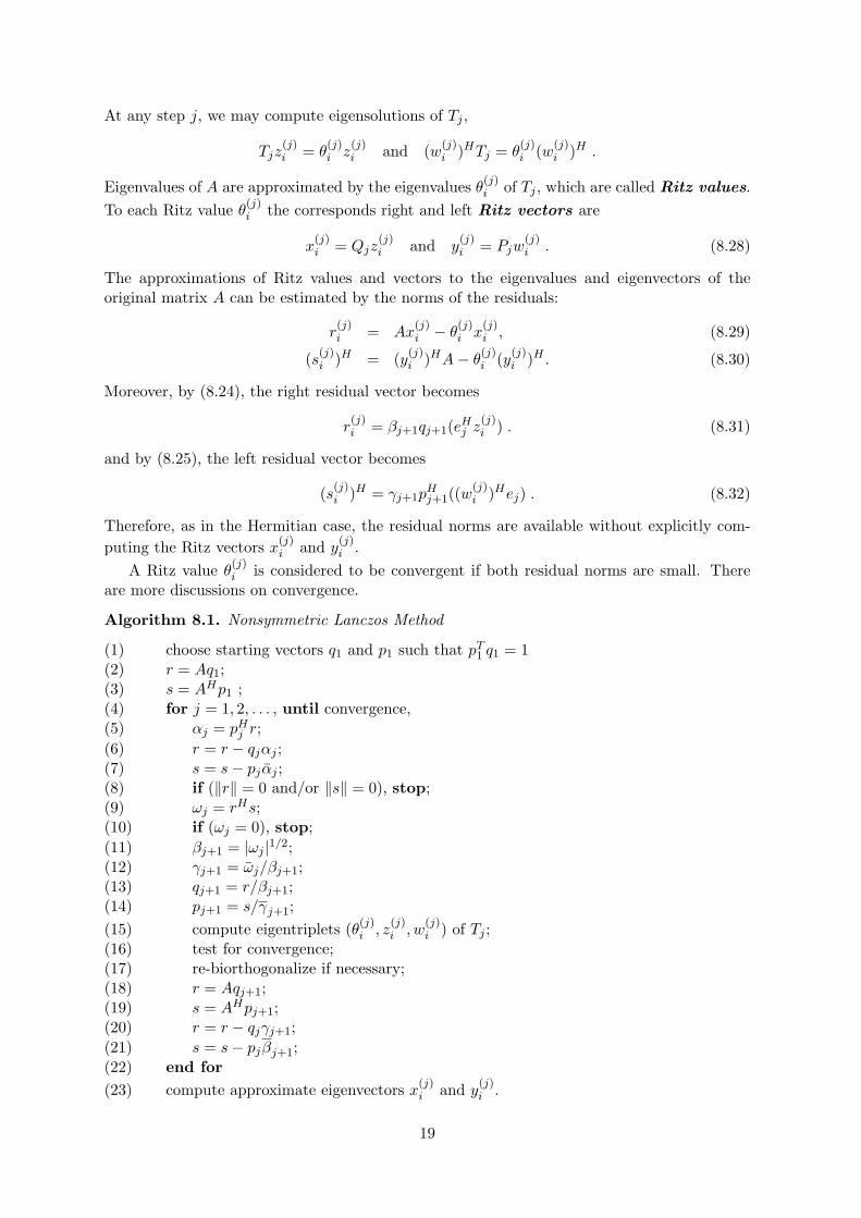
Algorithm 8.1. Nonsymmetric Lanczos Method
(1) choose starting vectors q1 and p1 such that pT1 q1 = 1
(2) r = Aq1;(3) s = AHp1 ;(4) for j = 1, 2, . . . , until convergence,(5) αj = pH
j r;
(6) r = r − qjαj ;(7) s = s − pjαj ;(8) if (‖r‖ = 0 and/or ‖s‖ = 0), stop;(9) ωj = rHs;(10) if (ωj = 0), stop;
(11) βj+1 = |ωj |1/2;(12) γj+1 = ωj/βj+1;(13) qj+1 = r/βj+1;(14) pj+1 = s/γj+1;
(15) compute eigentriplets (θ(j)i , z
(j)i , w
(j)i ) of Tj ;
(16) test for convergence;(17) re-biorthogonalize if necessary;(18) r = Aqj+1;(19) s = AHpj+1;(20) r = r − qjγj+1;
(21) s = s − pjβj+1;
(22) end for
(23) compute approximate eigenvectors x(j)i and y
(j)i .
19

We now comment on some of the steps in Algorithm 8.1:
(1) The initial starting vectors p1 and q1 are best selected by the user to embody any availableknowledge concerning A’s wanted eigenvectors. In the absence of such knowledge, onemay simply choose q1 with randomly distributed entries and let p1 = q1.
(2), (3) and (18), (19) The matrix-vector multiplication routines for Az and AHz of an arbi-trary vector z must be provided in these steps. These are usually the computationalbottleneck. See the discussion of convergence properties below for implementation notesin the shift-invert case.
(8) This is one of two cases where the method breaks down. In fact, this is a good breakdown.Say if r is null, then the Lanczos vectors {q1, q2, . . . , qj} span a (right) invariant subspaceof A. All eigenvalues of Tj are the eigenvalues of A. One can either exit the algorithm orcontinue the algorithm by taking the vector qj+1 to be any vector orthogonal to the leftLanczos vectors {p1, p2, . . . , pj} and set βj+1 = 0. Similar treatment can be done whens is null or both r and s are null. Therefore, this case should not really be regarded as a“failure” of the algorithm. It merely gives us freedom of choices.
In practice, an exact null vector is rare. It might happen that the norms of r and/or sare tiny. A proper tolerance value for the detection of nearly null vector should be given.A default tolerance value is ǫ, the machine precision.
(10) If ωj = rHs = 0 before either r or s vanishes, the method breaks down completely. Inmost cases we may continue finding new vectors in the Krylov subspaces Kj+k(A, r) andKj+k(AH , s) for some integer k > 0, and add a block outside the three diagonals of Tj ;this so-called a lookahead procedure as implemented in QMRPACK. If, however ourstarting vectors q1 and p1 have different minimal polynomials, even this does not help,and we have a mismatch, also called an incurable breakdown.
In practice, the exact breakdown is rare. A near breakdown occurs more often, i.e., ωj
is non-zero but extremely small in absolute value. Near breakdowns cause stagnation.Any criterion for detecting a near breakdown stops too early in certain applications andtoo late in others. A reasonable compromise criterion for detecting near breakdowns inan eigenvalue problem is to stop if |ωj | ≤
√ǫ‖r‖2‖s‖2.
(11) – (14) Several different scalings of the vectors qj and pj have been proposed. Here qj andpj are scaled such that pH
j qj = 1 for all j. Specifically, βj and γj are given equal absolutevalues, and the sub-diagonals βj are taken real and positive. The choice βj = 1 avoidsscaling the pj vectors, but unfortunately is highly susceptible to overflow. The choiceof βj = γj =
√ωj leads to a complex symmetric tridiagonal matrix Tj . The choice of
scaling such that the vectors qj and pj have unity norms is also a popular alternative.
The condition numbers of the Lanczos vectors Qj and Pj can be monitored by the scalars{ωi}. In fact, it can be shown that
cond(Qj) = ‖Qj‖2‖Q†j‖2 ≤
j∑
i=1
ω−1i ,
where Q†j denotes the generalized inverse of Qj . The bound also applies to cond(Pj).
(15) For each step j, the eigen-decomposition of the tridiagonal matrix Tj (8.27) is computed,which is potentially very costly when j gets large. A simple way to reduce the cost is tosolve the eigen-problem periodically, say every 10 steps.
20
One may use the general QR method to compute the eigensolution of Tj . If the scaling ischosen so that Tj is a complex symmetric tridiagonal matrix, a QL algorithm is availablethat exploits this special structure. However, due to the loss of unitary transformationin the QL algorithm, care must be taken to monitor and maintain numerical stability;
(16) Computation halts once bases Qj and Pj have been determined so that eigenvalues θ(j)i
of Tj (8.27) approximate all the desired eigenvalues of A with small residuals, which arecalculated according to the equations (8.31) and (8.32). There are more discussions onconvergence properties later.
If there is no re-biorthogonalization, then in finite precision arithmetic after a Ritz valueconverges to an eigenvalue of A, copies of this Ritz value may appear at later Lanczossteps. For example, a cluster of Ritz values of the reduced tridiagonal matrix, Tj , mayapproximate a single eigenvalue of the original matrix A. A “spurious” value is a simpleRitz value that is also an eigenvalue of the matrix of order j − 1 obtained by deletingthe first row and column from Tj . Such spurious value should be discarded from con-sideration. Eigenvalues of Tj which are not “spurious” are accepted as approximationsto eigenvalues of the original matrix A and are tested for convergence. It is called theidentification test.
(17) As in the Hermitian case, in the presence of finite precision arithmetic, the computedLanczos vectors {qi} and {pi} starts to lose the biorthogonality quickly. One may usethe two-sided modified Gram-Schmidt process to re-biorthogonalize them. Specifically,the following loop may be applied at this step:
for i = 1, 2, . . . , jqj+1 = qj+1 − qi(p
Hi qj+1);
pj+1 = pj+1 − pi(qHi pj+1);
end for
This is called the full re-biorthogonalization. However, it is in general very costly interms of memory references and flops, and becomes a computational bottleneck.
(23) The approximate eigenvectors of the original matrix A are only calculated after the test
in step (16) indicates convergence of Ritz values θ(j)i to the desired eigenvalues of A.
The bases Qj and Pj are used to get the approximate eigenvectors x(j)i = Qjz
(j)i and
y(j)i = Pjw
(j)i for each i that is flagged as converged.
The residuals (8.29) and (8.30) should be checked again using x(j)i and y
(j)i . This is the
actual residual norms. Note that the actual norms can be much bigger than the estimatedones computed at step (16).
It is adviced to compute approximate eigenvectors x(j)i and y
(j)i using the computed
Lanczos vectors Qj and Pj only if a certain level of biorthogonality is enforced in theimplementation of the algorithm (see step (17)).
Convergence properties. A theory of convergence can be based on the theory of polynomi-als as in the Hermitian case, but with two additional complications. First the eigenvalues may
be complex, and the Ritz values θ(j)i do not necessarily move monotonously out towards the
ends of the spectrum with increasing j. Second A may be defective (possessing an eigenvaluewhose algebraic multiplicity is strictly greater than its geometric multiplicity). Assuming exactcomputation, the tridiagonal matrix Tj is also defective after a sufficient number of steps j.
21
In floating point computation with machine precision ǫ, an eigenvalue of multiplicity m is per-turbed by up to O(ǫ1/m), which is much larger than ǫ for m > 1. Barring these complications,eigenvalues that are peripheral in the spectrum, seen as a set in the complex plane, convergefirst.
An inherent difficulty of a non-Hermitian eigen-problem is that there is no practically com-
putable bound on the distance from θ(j)i to an eigenvalue of A. It is possible though to bound
the distance, ‖F‖, to the nearest matrix, A − F , with eigen-triplet (θ(j)i , x
(j)i , y
(j)i ). Approx-
imate information about both left and right eigenvectors has many uses, such as revealing
the conditioning (or sensitivity) of an eigenvalue. Recall that residual vectors r(j)i and s
(j)i as
defined in (8.29) and (8.30). Next observe that the biorthogonality condition (8.26) implies
that (s(j)i )Hx
(j)i = (y
(j)i )Hr
(j)i = 0. Together these relations imply that
F =r(j)i (x
(j)i )H
‖x(j)i ‖2
2
+y
(j)i (s
(j)i )H
‖y(j)i ‖2
2
(8.33)
is the desired perturbation such that
(A − F )x(j)i = x
(j)i θ
(j)i , (8.34)
(y(j)i )H(A − F ) = θ
(j)i (y
(j)i )H , (8.35)
and ‖F‖2F = ‖r(j)
i ‖22/‖x
(j)i ‖2
2 + ‖s(j)i ‖2
2/‖y(j)i ‖2
2. Using the standard perturbation analysis, onecan derive estimated error bounds on the accuracy of approximate eigenvalues and eigenvectorsto the exact eigenvalues and eigenvectors of A. To this end, we should point out all these resultsare under the assumption of exact arithmetic. In the presence of finite precision arithmeticand the losses in biorthogonality, those results are generally optimistic.
9 Symmetric definite eigenvalue problems
Most iterative methods for solving large sparse standard eigenvalue problem, such as Lanczosmethod and Arnoldi method, can be modified to treat the generalized eigenvalue problems.Let us focus on the generalized symmetric definite eigenvalue problem, namely Ax = λBx,where A and B are symmetric, and B is positive definite.
If we can compute the sparse Cholesky factorization of B explicitly, then as shown in theprevious section, it is equivalent solve the standard symmetric eigenvalue problem
Cy = λy ⇐⇒ (L−1AL−H)(LHx) = λ(LHx).
One can use the Lanczos method for C. It is straightforward.Note that the required matrix-vector multiplication w = Cq for some q in the Lanczos
process can be done in the following three stages:
1. solve LHz1 = q1 for z1;2. compute z2 = Az1;3. solve Lw = z2 for w.
This approach is usually very satisfactory and is a standard working practice, particularly,when B is a banded matrix with narrow bandwidth.
On the other hand it is possible to use Lanczos on B−1A, again implicitly. This option isvaluable when B cannot be factored conveniently. In this case, the Lanczos method must bereformulated.
22

First note that the matrix B−1A is symmetric with respect to B, namely,
〈B−1Ax, y〉B = 〈x, B−1Ay〉B,
where the inner product 〈x, y〉B is defined as yT Bx, known as B-inner product. ‖ · ‖B is thecorresponding B-norm ‖x‖B =
√xT Bx.
Mathematically the extension of the Lanczos process in B-inner product is immediate:
Algorithm 9.1 (Lanczos Process in B-inner product for B−1A).1. q1 = v/‖v‖B, β0 = 0; q0 = 0;2. for j = 1 to k, do3. w = B−1Aqj ;4. αj = 〈w, qj〉B;5. w = w − αjqj − βj−1qj−1;6. βj = ‖w‖B;7. if βj = 0, quit;8. qj+1 = w/βj ;9. EndDo
The governing relations are B−1AQk = QkTk + βkqk+1eTk , or
AQk = BQkTk + βkBqk+1eTk , (9.36)
andQT
k BQk = Ik, QTk Bqk+1 = 0. (9.37)
Let µ be an eigenvalue of Tk and y be the corresponding eigenvector y, i.e.,
Tky = µy, ‖y‖2 = 1.
Then applying y to the right hand side of (9.36), we have
AQky = BQkTky + βkBqk+1eTk y = µBQky + βkBqk+1e
Tk y.
The Ritz value is µ and the Ritz vector is Qky. The residual vector r is
r = AQky − µBQky = βkBqk+1(eTk y).
The norm of residual vector can be used as a stopping criterion.We now show that the above Lanczos process can be further simplified. Note that
1. αj = 〈w, qj〉B = qTj Bw = qT
j BB−1Aqj = qTj Aqj , and
2. ‖w‖2B = wT Bw = wT (Aqj −αjBqj −βj−1Bqj−1) = wT Aqj . The last equality is obtained
by the fact that w(= βjqj+1) is generated to be B-orthogonal to all previous Lanczosvectors q1, q2, . . . , qj .
In summary, we have the following Lanczos method for the eigenvalue problem of a definitepencil A − λB with positive definite B.
Algorithm 9.2 (Lanczos Algorithm for a symmetric definite pair (A, B)).1. choose an initial vector q1 of B-norm unity;2. for j = 1 to k, do3. v = Aqj ;4. αj = qT
j v;
5. w = B−1v − αjqj − βj−1qj−1;
23

6. βj =√
wT v;7. if βj = 0, quit (an invariant subspace found);8. qj+1 = w/βj ;9. Compute eigenvalues and eigenvectors of Tj ;10. Test for convergence;11. EndDo
Shift-and-invert spectral transformation. The above two approaches are efficient if onlythe exterior eigenvalues are sought. If the interesting eigenvalues are interior ones, then thecommon approach is to first use the shift-and-invert spectral transformation. Let σ is a shiftwhich close to the desired eigenvalues. Then the generalized eigenvalue problem Ax = λBx isequivalent to
[(A − σB)−1B
]x =
1
λ − σx.
Note that the coefficient matrix[(A − σB)−1B
]is B-symmetric.
Exercises
9.1. Verify that 〈x, y〉B is an inner product, where B is symmetric positive definite.
10 Further reading
Krylov subspace projection methods are covered extensively in
• Z. Bai, J. Demmel, J. Dongarra, A. Ruhe and H. van der Vorst (editors). Templates forthe Solution of Algebraic Eigenvalue Problems: A Practical Guide. SIAM, Philadelphia,2000.
The implicitly restarted Arnoldi method is proposed in
• D. Sorensen, Implicit application of polynomial filters in a k-step Arnoldi method,SIMAX, Vol. 13, pp.357–385, 1992.
MATLAB function eigs is an implementation of the implicitly restarted Arnoldi algorithm forfinding a few eigenpairs. The Fortran software package is ARPACK3. See
• R. Lehoucq, D. C. Sorensen and C. Yang. ARPACK User’s Guide, SIAM, 1998.
An excellent reference on symmetric Lanczos method, theory and practice, is
• B. N. Parlett, The Symmetric Eigenvalue Problem, reprinted (with some revision) bySIAM Press, 1998.
The thick restarting symmetric Lanczos algorithm is described in
• K. Wu and H. Simon, Thick-restart lanczos method for large symmetric eigenvalue prob-lems, SIAM J. Mat. Anal. Appl., 22:602–616, 2000.
A recent development can be found in
• I. Yamazaki, Z. Bai, H. Simon, L.-W. Wang and K. Wu, Adaptive projection subspacedimension for the thick-restart Lanczos method, 2009 (submitted)4
3http://www.caam.rice.edu/software/ARPACK4http://www.cs.ucdavis.edu/∼bai
24
A Fortran implementation of the nonsymmetric Lanczos procedure with look-ahead to curebreakdowns is available in QMRPACK5. The algorithm is described in
• R. Freund and N. Nachtigal. QMR: a quasi-minimal residual method for non-Hermitianlinear system, Numer. Math. 60:315–339,1991.
A set of MATLAB routines for implementing the adaptive block Lanczos method can be usedto implement Algorithm 8.1 by defining the blocksize as one at the initial step. Optionalre-biorthogonalization schemes are available. An adaptive blocksize scheme is used for thetreatment of (near) breakdown and/or multiple or closely clustered eigenvalues of interest. See
• Z. Bai, D. Day and Q. Ye, ABLE: an adaptive block Lanczos method for non-Hermitianeigenvalue problems, SIMAX, Vol.20, pp. 1060–1082, 1999.
5http://www.netlib/linalg/qmrpack.tgz
25
Recommended
![Deflation and augmentation techniques in Krylov …introduction to Krylov subspace methods and to [74] for a recent overview on Krylov subspace methods; see also [20, 21] for an advanced](https://img.pdfslide.us/doc/110x75/5edc1784ad6a402d66669cc6/deiation-and-augmentation-techniques-in-krylov-introduction-to-krylov-subspace.jpg)

![COMPUTING APPROXIMATE (BLOCK) RATIONAL ......Krylov subspace, as we have already shown for extended Krylov subspaces in [17]. Block Krylov subspace methods are an extension of Krylov](https://img.pdfslide.us/doc/110x75/5edc1787ad6a402d66669cca/computing-approximate-block-rational-krylov-subspace-as-we-have-already.jpg)