1
Before the
POSTAL REGULATORY COMMISSION WASHINGTON, DC 20268-0001
Institutional Cost Contribution Docket No. RM2017-1 Requirement for Competitive Products
ADDITIONAL DECLARATION OF SOILIOU DAW NAMORO FOR THE PUBLIC REPRESENTATIVE
(September 12, 2018)
I. Autobiographical Sketch
My name is Soiliou Daw Namoro. I am an economist with the Postal Regulatory
Commission (PRC), where I have been working since 2017. I hold a Ph.D. in
Economics (State University of New York, at Stony Brook) and a Ph.D. in Statistics
(Catholic University of Louvain, Louvain-la-Neuve, Belgium).
Before joining the PRC, I worked for more than a decade as a lecturer at the
University of Pittsburgh, Department of Economics, where I taught graduate-level
courses of Econometrics and Mathematics. I have sat on several Ph.D. thesis
committees. I also taught several undergraduate courses, such as Industrial
Organization, Health Economics, Development Economics, and Financial Markets and
other similar courses. I have conducted research in theoretical and applied
econometrics, applied microeconomics, health economics, and development
economics. I have published research articles in peer-review Journals, such as the
Journal of Econometrics and the Journal of Economics. I have contributed to books.
The latest contribution is co-authored with Margaret Cigno, Director of the Office of
Accountability and Compliance at the PRC and published in The Contribution of the
Postal Regulatory CommissionSubmitted 9/12/2018 10:33:25 AMFiling ID: 106505Accepted 9/12/2018
2
Postal and Delivery Sector: Between E-Commerce and E-Substitution (Topics in
Regulatory Economics and Policy).
II. Purpose of Declaration
The Public Representative tasked me with reviewing, analyzing and preparing
comments on my findings regarding the Commission’s formula proposed in Order No.
4742 to calculate the minimum contribution requirement to total institutional costs by the
Postal Service’s competitive products.
III. Declaration
1. Introduction and Outline
Upon its review of the Comments raised to the formula-based approach to setting
the appropriate share proposed in Order No. 44021, the Commission’s has proposed a
new equation to calculate the annual minimum contribution share by competitive
products to institutional costs. As its predecessor proposed in Order No. 4402,
henceforth referred to, for convenience, as the Order 4402 formula, the new equation
recursively updates the minimum contribution share computed for a given year to set
the minimum share for the following year. Using the minimum appropriate share
determined in 2006 of 5.5 percent for FY 2007 and FY 2008, the Commission starts
recalculation from FY 2009.
The content of the informational materials, specifically, the data and the statutory
guidelines, that underlie the new formula, is not substantially different from the materials
that were used by the Commission to develop and support the Order 4402 formula.
Consequently, although, as I will discuss later in the declaration, the new formula is, in
many respects, an improved version of the Order 4402 formula, the realized
1 Notice of Proposed Rulemaking to Evaluate the Institutional Cost Contribution Requirement for Competitive Products, February 8, 2018 (Order No. 4402).

3
improvement remains short of demonstrating that the ongoing appropriate share has
become inappropriate and, therefore, needs to be changed. Further, recent
developments in the delivery industry suggest that a careful review of the Commission’s
appropriate share regulation involves judgments which may not be accurately depicted
in a mathematical formula.2 The last statement should be qualified, however, by the
possibility for the Commission to revisit the proposed formula at any time in the future. I
also note the ability of the formula to absorb the most catastrophic down-turn of the
market from the Postal Service’s perspective, by reducing the appropriate share to the
stable value of zero until a new non-zero appropriate share is set by the Commission.
This point will be further developed in the part of the declaration that discusses the
stability of the formula.
The purpose of this declaration is to evaluate the new formula. This evaluation is
guided by the precept that the formula must enable the Commission to decide about the
appropriate share based on incomplete information and in the presence of unforeseen
events. It consequently focuses on the following points:
The Reasoning Behind the new formula.
Are there other implicit reasons than those presented by the Commission to design the
formula that need to be made explicit? Does this reasoning provide additional ground
for using the formula as a decision-making tool suited to its intended use?
The stability of the formula: how likely is the formula to generate shares that change
dramatically with unpredictable time patterns? How likely is it to produce long-lasting
and self-sustaining trends of shares, which ultimately end in one of the two extreme
values of the shares, 0 and 1?
These points are informally developed as follows:
2 The complexity of the involved judgments is not unlike the one regarding pricing described in Docket R87-1, Opinion and Recommended Decision, March 4, 1988, Vol 1, at 360. Noticeable in this respect is the fact reported by the Wall Street Journal that Amazon is “inviting entrepreneurs to form small delivery in a continued quest to build a vast freight and parcel shipping network.” This move by the online retail giant further strengthens its position as a strategic player in the delivery market with large monopsonistic powers. The evolution could, if it amplifies, have a major impact on the development of the structure of the package delivery industry, and increase market uncertainty, a challenge already faced by the Postal Service, whose financial sustainability continues to erode, according to the Commission’s financial analysis for the fiscal year 2017. See PRC, FINANCIAL ANALYSIS of United States Postal Service Financial Results and 10-K Statement, Fiscal Year 2017, April 5, 2018, at 6.

4
Much intuition can be gained about the new formula if one takes the Commission’s
Competitive Contribution Margin (CCM) for what it effectively is: the percentage of
gross sales revenue available to cover (or contribute to) institutional costs. Hence,
changes in this ratio, or in its absolute counterpart, the numerator of the CCM,
measure in relative and absolute terms, possibly imperfectly, the joint ability of the
Postal Service’s competitive products to contribute to the coverage of institutional
costs. I refer, in short, to this capability as the Postal Service’s ability to pay.
Based on this interpretation of the CCM, I establish that the new formula’s updating
rule can be summarized as follows:
Raise (reduce) the minimum share for the next fiscal year if the Postal Service’s
ability to pay has increased (decreased) faster than a reference baseline this year,
compared to the last. This rule is shown in two alternative but equivalent versions.
While the rule is intuitively sound, it nevertheless raises an important question
regarding the principles guiding the Commission’s minimum-share updating policy:
Should any relative increase in the Postal Service’s ability to pay be automatically
construed as an increase in its obligation to pay? A similar question can, of course, be
asked about relative decreases in the Postal Service’s ability to pay.
To the best of my reading of Order No. 4742, these questions are not addressed
therein, but they essentially concern the degree of flexibility that the Postal Service has,
or ought to have, in conducting its business within its statutory scope.
The fear that the formula could generate patterns of shares that change dramatically
over time is among the reasons for worrying about stability. However, the word
“stability” applied to a recursive discrete-time, or to a differential equation, has
several different meanings and the omission to properly define the sense in which
one uses this word may generate confusion where the policy debate needs clarity.
For example, the popular notion of Lyapunov stability applies to equilibrium points of
the recursion. In the present case, there is a unique equilibrium, the zero share, and
5
stability of this equilibrium point means the wandering of the computed shares
towards zero. Some stakeholders may find the property very attractive if it holds.
Others may dislike it very much. As it pertains to the Commission’s formula,
Lyapunov stability cannot be proved or disproved theoretically without making
questionable assumptions on the dynamics of the Postal Service’s ability to pay.
Because, in the present case, any formal proof of stability – or lack of stability –
cannot avoid relying on unverifiable assumptions on the likely time path of the Postal
Service’s ability to pay, I provide simulation results based on the assumption that
the rate of change in the share can only take the lowest or highest value observed
over the period 2007-2017.
Regarding the likely behavior of the computed shares in the long run, I discuss the
meaning of the eventual convergence of the shares to a limit when the time tends to
infinity. Intuitively, this simply means that the shares eventually become arbitrarily
close to one another. I provide necessary conditions, as well as sufficient conditions,
for the convergence. These conditions show that, here also, convergence cannot be
proved or disproved without making questionable assumptions on the dynamics of
the Postal Service’s ability to pay.
As for the possibility of unpredictable erratic trends in the computed shares, I stress
the fact that the indexation – in the formula – of the change in the appropriate share
to the change in the Postal Service’s ability to pay implies that the computed shares
and the Postal Service’s ability have exactly the same time-trends. Hence, predicting
the time-trends in the first amounts to predicting the trends in the second. I discuss
the latter trends by focusing on product-specific price-to-unit-cost ratios and the price
ratios between the Postal Service and its competitors.
2. Evaluation of the New Formula
The Commission’s new formula is stated as
6
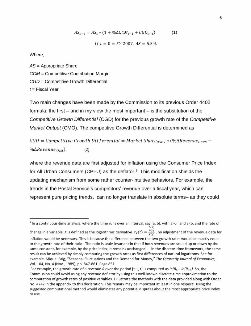
𝐴𝑆𝑡+1 = 𝐴𝑆𝑡 ∗ (1 + %∆𝐶𝐶𝑀𝑡−1 + 𝐶𝐺𝐷𝑡−1) (1)
𝐼𝑓 𝑡 = 0 = 𝐹𝑌 2007, 𝐴𝑆 = 5.5%
Where,
AS = Appropriate Share
CCM = Competitive Contribution Margin
CGD = Competitive Growth Differential
t = Fiscal Year
Two main changes have been made by the Commission to its previous Order 4402
formula: the first – and in my view the most important – is the substitution of the
Competitive Growth Differential (CGD) for the previous growth rate of the Competitive
Market Output (CMO). The competitive Growth Differential is determined as
𝐶𝐺𝐷 = 𝐶𝑜𝑚𝑝𝑒𝑡𝑖𝑡𝑖𝑣𝑒 𝐺𝑟𝑜𝑤𝑡ℎ 𝐷𝑖𝑓𝑓𝑒𝑟𝑒𝑛𝑡𝑖𝑎𝑙 = 𝑀𝑎𝑟𝑘𝑒𝑡 𝑆ℎ𝑎𝑟𝑒𝑈𝑆𝑃𝑆 ∗ (%∆𝑅𝑒𝑣𝑒𝑛𝑢𝑒𝑈𝑆𝑃𝑆 −
%∆𝑅𝑒𝑣𝑒𝑛𝑢𝑒𝐶&𝑀), (2)
where the revenue data are first adjusted for inflation using the Consumer Price Index
for All Urban Consumers (CPI-U) as the deflator.3 This modification shields the
updating mechanism from some rather counter-intuitive behaviors. For example, the
trends in the Postal Service’s competitors’ revenue over a fiscal year, which can
represent pure pricing trends, can no longer translate in absolute terms– as they could
3 In a continuous-time analysis, where the time runs over an interval, say [a, b], with a>0, and a<b, and the rate of
change in a variable X is defined as the logarithmic derivative 𝑟𝑋(𝑡) =
𝜕(𝑋)
𝜕(𝑡)
𝑋(𝑡) , no adjustment of the revenue data for
inflation would be necessary. This is because the difference between the two growth rates would be exactly equal to the growth rate of their ratio. The ratio is scale-invariant in that if both revenues are scaled up or down by the same constant, for example, by the price index, it remains unchanged. In the discrete-time framework, the same result can be achieved by simply computing the growth rates as first differences of natural logarithms. See for example, Miquel Faig, “Seasonal Fluctuations and the Demand for Money,” The Quarterly Journal of Economics, Vol. 104, No. 4 (Nov., 1989), pp. 847-861. Page 851. For example, the growth rate of a revenue R over the period [t-1, t] is computed as ln(Rt ) –ln(Rt-1 ). So, the Commission could avoid using any revenue deflator by using this well-known discrete-time approximation to the computation of growth rates of positive variables. I illustrate the methods with the data provided along with Order No. 4742 in the appendix to this declaration. This remark may be important at least in one respect: using the suggested computational method would eliminates any potential disputes about the most appropriate price index to use.
7
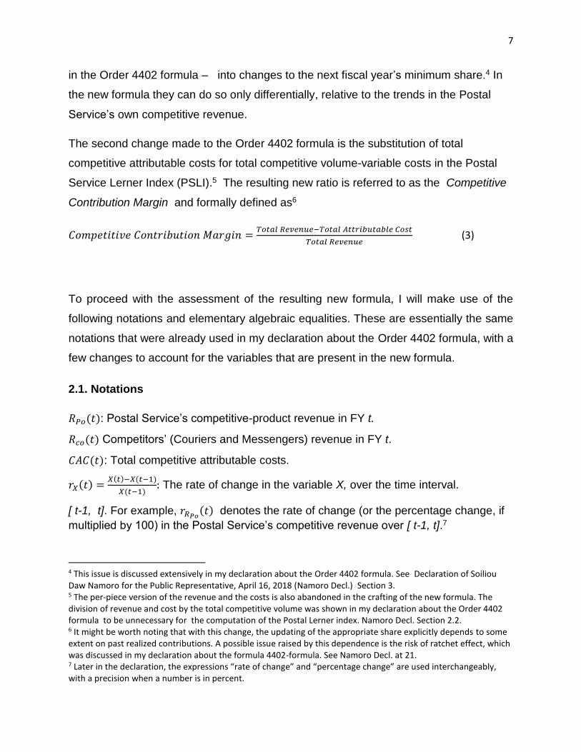
in the Order 4402 formula – into changes to the next fiscal year’s minimum share.4 In
the new formula they can do so only differentially, relative to the trends in the Postal
Service’s own competitive revenue.
The second change made to the Order 4402 formula is the substitution of total
competitive attributable costs for total competitive volume-variable costs in the Postal
Service Lerner Index (PSLI).5 The resulting new ratio is referred to as the Competitive
Contribution Margin and formally defined as6
𝐶𝑜𝑚𝑝𝑒𝑡𝑖𝑡𝑖𝑣𝑒 𝐶𝑜𝑛𝑡𝑟𝑖𝑏𝑢𝑡𝑖𝑜𝑛 𝑀𝑎𝑟𝑔𝑖𝑛 =𝑇𝑜𝑡𝑎𝑙 𝑅𝑒𝑣𝑒𝑛𝑢𝑒−𝑇𝑜𝑡𝑎𝑙 𝐴𝑡𝑡𝑟𝑖𝑏𝑢𝑡𝑎𝑏𝑙𝑒 𝐶𝑜𝑠𝑡
𝑇𝑜𝑡𝑎𝑙 𝑅𝑒𝑣𝑒𝑛𝑢𝑒 (3)
To proceed with the assessment of the resulting new formula, I will make use of the
following notations and elementary algebraic equalities. These are essentially the same
notations that were already used in my declaration about the Order 4402 formula, with a
few changes to account for the variables that are present in the new formula.
2.1. Notations
𝑅𝑃𝑜(𝑡): Postal Service’s competitive-product revenue in FY t.
𝑅𝑐𝑜(𝑡) Competitors’ (Couriers and Messengers) revenue in FY t.
𝐶𝐴𝐶(𝑡): Total competitive attributable costs.
𝑟𝑋(𝑡) =𝑋(𝑡)−𝑋(𝑡−1)
𝑋(𝑡−1): The rate of change in the variable X, over the time interval.
[ t-1, t]. For example, 𝑟𝑅𝑃𝑜(𝑡) denotes the rate of change (or the percentage change, if
multiplied by 100) in the Postal Service’s competitive revenue over [ t-1, t].7
4 This issue is discussed extensively in my declaration about the Order 4402 formula. See Declaration of Soiliou Daw Namoro for the Public Representative, April 16, 2018 (Namoro Decl.) Section 3. 5 The per-piece version of the revenue and the costs is also abandoned in the crafting of the new formula. The division of revenue and cost by the total competitive volume was shown in my declaration about the Order 4402 formula to be unnecessary for the computation of the Postal Lerner index. Namoro Decl. Section 2.2. 6 It might be worth noting that with this change, the updating of the appropriate share explicitly depends to some extent on past realized contributions. A possible issue raised by this dependence is the risk of ratchet effect, which was discussed in my declaration about the formula 4402-formula. See Namoro Decl. at 21. 7 Later in the declaration, the expressions “rate of change” and “percentage change” are used interchangeably, with a precision when a number is in percent.
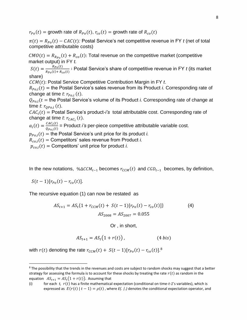
8
𝑟𝑃𝑜(𝑡) = growth rate of 𝑅𝑃𝑜(𝑡), 𝑟𝑐𝑜(𝑡) = growth rate of 𝑅𝑐𝑜(𝑡)
𝜋(𝑡) = 𝑅𝑃𝑜(𝑡) − 𝐶𝐴𝐶(𝑡): Postal Service’s net competitive revenue in FY t (net of total competitive attributable costs)
𝐶𝑀𝑂(𝑡) = 𝑅𝑅𝑃𝑜(𝑡) + 𝑅𝑐𝑜(𝑡): Total revenue on the competitive market (competitive
market output) in FY t.
𝑆(𝑡) =𝑅𝑃𝑜(𝑡)
𝑅𝑃𝑜(𝑡)+ 𝑅𝑐𝑜(𝑡)∶ Postal Service’s share of competitive revenue in FY t (its market
share) 𝐶𝐶𝑀(𝑡): Postal Service Competitive Contribution Margin in FY t.
𝑅𝑃𝑜,𝑖(𝑡) = the Postal Service’s sales revenue from its Product i. Corresponding rate of
change at time t: 𝑟𝑃𝑜,𝑖 (𝑡). 𝑄𝑃𝑜,𝑖(𝑡 = the Postal Service’s volume of its Product i. Corresponding rate of change at
time t: 𝑟𝑄𝑃𝑜,𝑖 (𝑡).
𝐶𝐴𝐶𝑖(𝑡) = Postal Service’s product-i’s total attributable cost. Corresponding rate of change at time t: 𝑟𝐶𝐴𝐶𝑖 (𝑡).
𝑎𝑖(𝑡) =𝐶𝐴𝐶𝑖(𝑡)
𝑄𝑃𝑜,𝑖(𝑡) = Product i’s per-piece competitive attributable variable cost.
𝑝𝑃𝑜,𝑖(𝑡) = the Postal Service’s unit price for its product i.
𝑅𝑐𝑜,𝑖(𝑡) = Competitors’ sales revenue from Product i.
𝑝𝑐𝑜,𝑖(𝑡) = Competitors’ unit price for product i.
In the new notations, %∆𝐶𝐶𝑀𝑡−1 becomes 𝑟𝐶𝐶𝑀(𝑡) and 𝐶𝐺𝐷𝑡−1 becomes, by definition,
𝑆(𝑡 − 1)[𝑟𝑃𝑜(𝑡) − 𝑟𝑐𝑜(𝑡)].
The recursive equation (1) can now be restated as
𝐴𝑆𝑡+1 = 𝐴𝑆𝑡{1 + 𝑟𝐶𝐶𝑀(𝑡) + 𝑆(𝑡 − 1)[𝑟𝑃𝑜(𝑡) − 𝑟𝑐𝑜(𝑡)]} (4)
𝐴𝑆2008 = 𝐴𝑆2007 = 0.055
Or , in short,
𝐴𝑆𝑡+1 = 𝐴𝑆𝑡(1 + 𝑟(𝑡)) , (4 𝑏𝑖𝑠)
with 𝑟(𝑡) denoting the rate 𝑟𝐶𝐶𝑀(𝑡) + 𝑆(𝑡 − 1)[𝑟𝑃𝑜(𝑡) − 𝑟𝑐𝑜(𝑡)].8
8 The possibility that the trends in the revenues and costs are subject to random shocks may suggest that a better strategy for assessing the formula is to account for these shocks by treating the rate 𝑟(𝑡) as random in the
equation 𝐴𝑆𝑡+1 = 𝐴𝑆𝑡(1 + 𝑟(𝑡)). Assuming that
(i) for each t, 𝑟(𝑡) has a finite mathematical expectation (conditional on time-t-1’s variables), which is expressed as 𝐸(𝑟(𝑡) | 𝑡 − 1) = 𝜌(𝑡) , where E(. |.) denotes the conditional expectation operator, and
9
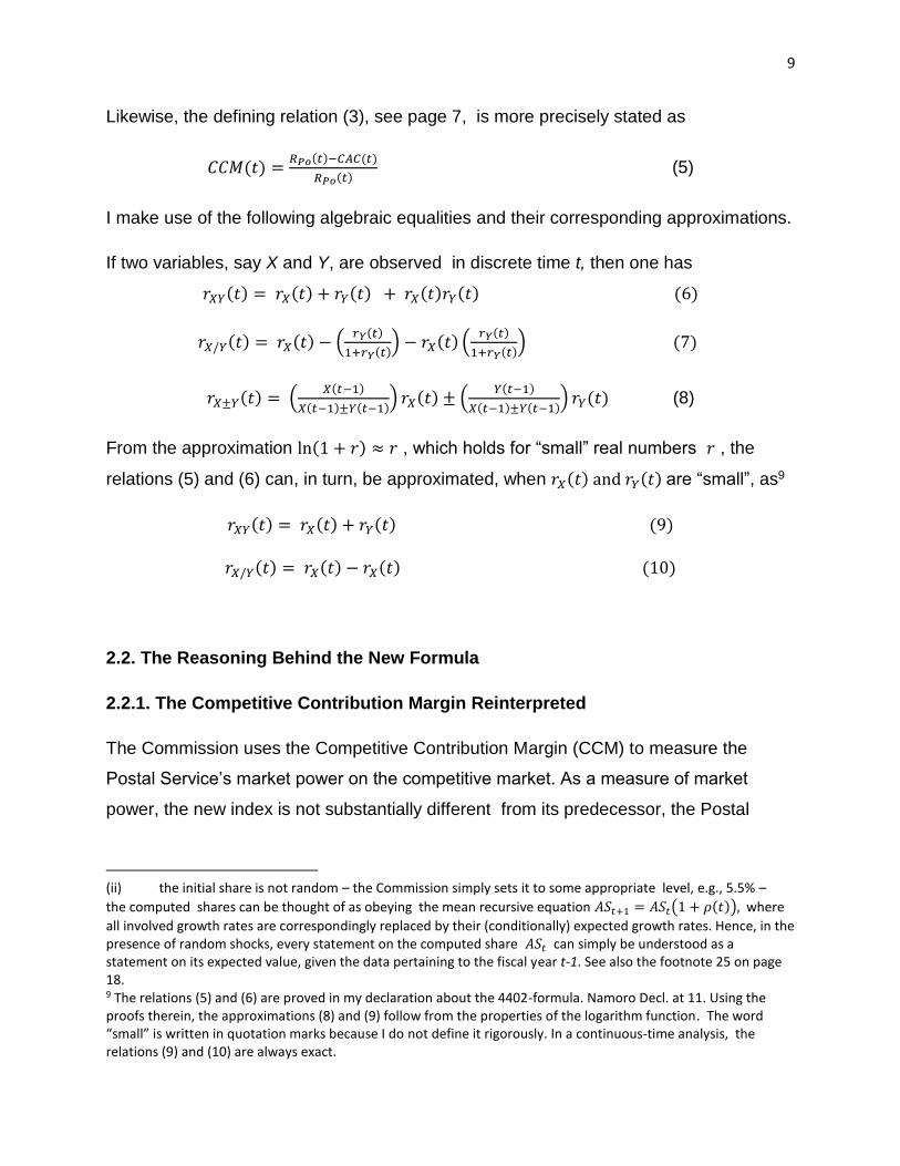
Likewise, the defining relation (3), see page 7, is more precisely stated as
𝐶𝐶𝑀(𝑡) =𝑅𝑃𝑜(𝑡)−𝐶𝐴𝐶(𝑡)
𝑅𝑃𝑜(𝑡) (5)
I make use of the following algebraic equalities and their corresponding approximations.
If two variables, say X and Y, are observed in discrete time t, then one has
𝑟𝑋𝑌(𝑡) = 𝑟𝑋(𝑡) + 𝑟𝑌(𝑡) + 𝑟𝑋(𝑡)𝑟𝑌(𝑡) (6)
𝑟𝑋/𝑌(𝑡) = 𝑟𝑋(𝑡) − (𝑟𝑌(𝑡)
1+𝑟𝑌(𝑡)) − 𝑟𝑋(𝑡) (
𝑟𝑌(𝑡)
1+𝑟𝑌(𝑡)) (7)
𝑟𝑋±𝑌(𝑡) = (𝑋(𝑡−1)
𝑋(𝑡−1)±𝑌(𝑡−1)) 𝑟𝑋(𝑡) ± (
𝑌(𝑡−1)
𝑋(𝑡−1)±𝑌(𝑡−1)) 𝑟𝑌(𝑡) (8)
From the approximation ln(1 + 𝑟) ≈ 𝑟 , which holds for “small” real numbers 𝑟 , the
relations (5) and (6) can, in turn, be approximated, when 𝑟𝑋(𝑡) and 𝑟𝑌(𝑡) are “small”, as9
𝑟𝑋𝑌(𝑡) = 𝑟𝑋(𝑡) + 𝑟𝑌(𝑡) (9)
𝑟𝑋/𝑌(𝑡) = 𝑟𝑋(𝑡) − 𝑟𝑋(𝑡) (10)
2.2. The Reasoning Behind the New Formula
2.2.1. The Competitive Contribution Margin Reinterpreted
The Commission uses the Competitive Contribution Margin (CCM) to measure the
Postal Service’s market power on the competitive market. As a measure of market
power, the new index is not substantially different from its predecessor, the Postal
(ii) the initial share is not random – the Commission simply sets it to some appropriate level, e.g., 5.5% –
the computed shares can be thought of as obeying the mean recursive equation 𝐴𝑆𝑡+1 = 𝐴𝑆𝑡(1 + 𝜌(𝑡)), where
all involved growth rates are correspondingly replaced by their (conditionally) expected growth rates. Hence, in the presence of random shocks, every statement on the computed share 𝐴𝑆𝑡 can simply be understood as a statement on its expected value, given the data pertaining to the fiscal year t-1. See also the footnote 25 on page 18. 9 The relations (5) and (6) are proved in my declaration about the 4402-formula. Namoro Decl. at 11. Using the proofs therein, the approximations (8) and (9) follow from the properties of the logarithm function. The word “small” is written in quotation marks because I do not define it rigorously. In a continuous-time analysis, the relations (9) and (10) are always exact.
10
Service Lerner index (PSLI). Hence, my remarks about this use of the CCM are the
same as the ones I formulated about the PSLI in my declaration about the Order 4402
formula.10
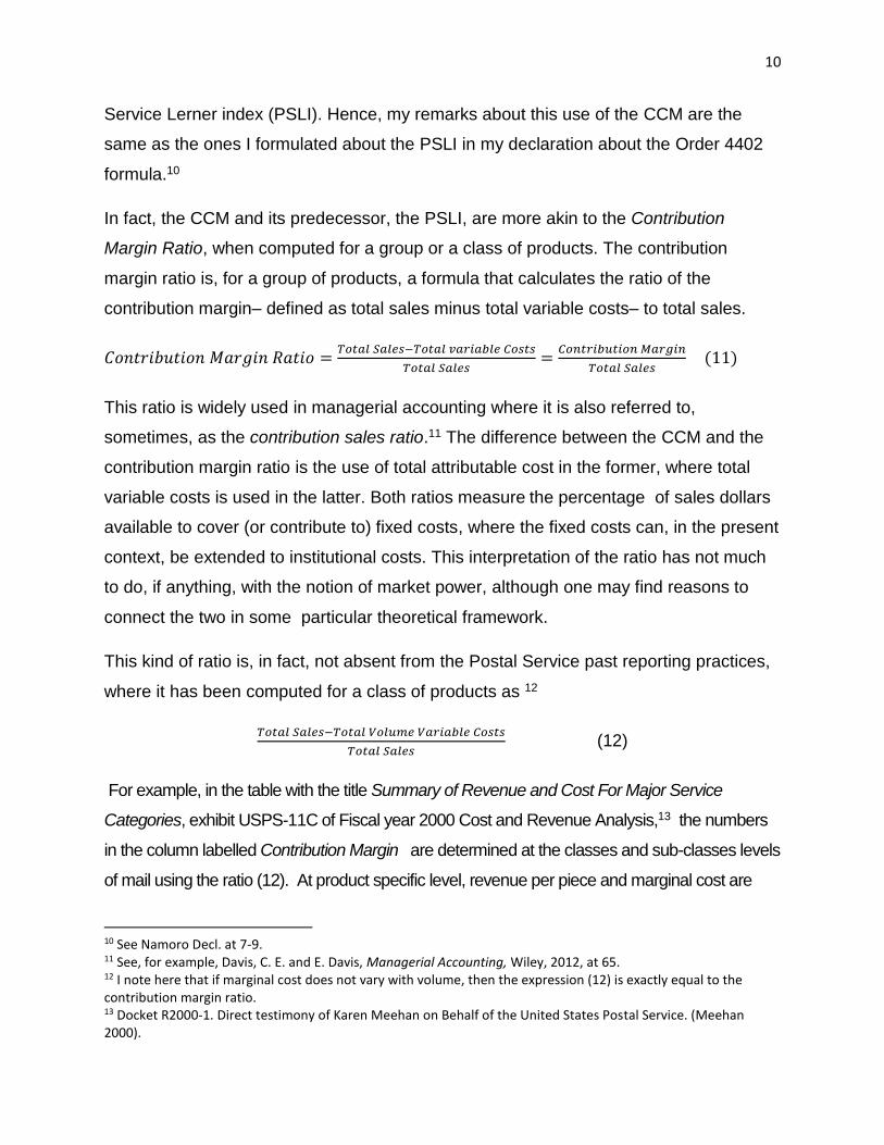
In fact, the CCM and its predecessor, the PSLI, are more akin to the Contribution
Margin Ratio, when computed for a group or a class of products. The contribution
margin ratio is, for a group of products, a formula that calculates the ratio of the
contribution margin– defined as total sales minus total variable costs– to total sales.
𝐶𝑜𝑛𝑡𝑟𝑖𝑏𝑢𝑡𝑖𝑜𝑛 𝑀𝑎𝑟𝑔𝑖𝑛 𝑅𝑎𝑡𝑖𝑜 =𝑇𝑜𝑡𝑎𝑙 𝑆𝑎𝑙𝑒𝑠−𝑇𝑜𝑡𝑎𝑙 𝑣𝑎𝑟𝑖𝑎𝑏𝑙𝑒 𝐶𝑜𝑠𝑡𝑠
𝑇𝑜𝑡𝑎𝑙 𝑆𝑎𝑙𝑒𝑠=
𝐶𝑜𝑛𝑡𝑟𝑖𝑏𝑢𝑡𝑖𝑜𝑛 𝑀𝑎𝑟𝑔𝑖𝑛
𝑇𝑜𝑡𝑎𝑙 𝑆𝑎𝑙𝑒𝑠 (11)
This ratio is widely used in managerial accounting where it is also referred to,
sometimes, as the contribution sales ratio.11 The difference between the CCM and the
contribution margin ratio is the use of total attributable cost in the former, where total
variable costs is used in the latter. Both ratios measure the percentage of sales dollars
available to cover (or contribute to) fixed costs, where the fixed costs can, in the present
context, be extended to institutional costs. This interpretation of the ratio has not much
to do, if anything, with the notion of market power, although one may find reasons to
connect the two in some particular theoretical framework.
This kind of ratio is, in fact, not absent from the Postal Service past reporting practices,
where it has been computed for a class of products as 12
𝑇𝑜𝑡𝑎𝑙 𝑆𝑎𝑙𝑒𝑠−𝑇𝑜𝑡𝑎𝑙 𝑉𝑜𝑙𝑢𝑚𝑒 𝑉𝑎𝑟𝑖𝑎𝑏𝑙𝑒 𝐶𝑜𝑠𝑡𝑠
𝑇𝑜𝑡𝑎𝑙 𝑆𝑎𝑙𝑒𝑠 (12)
For example, in the table with the title Summary of Revenue and Cost For Major Service
Categories, exhibit USPS-11C of Fiscal year 2000 Cost and Revenue Analysis,13 the numbers
in the column labelled Contribution Margin are determined at the classes and sub-classes levels
of mail using the ratio (12). At product specific level, revenue per piece and marginal cost are
10 See Namoro Decl. at 7-9. 11 See, for example, Davis, C. E. and E. Davis, Managerial Accounting, Wiley, 2012, at 65. 12 I note here that if marginal cost does not vary with volume, then the expression (12) is exactly equal to the contribution margin ratio. 13 Docket R2000-1. Direct testimony of Karen Meehan on Behalf of the United States Postal Service. (Meehan 2000).
11
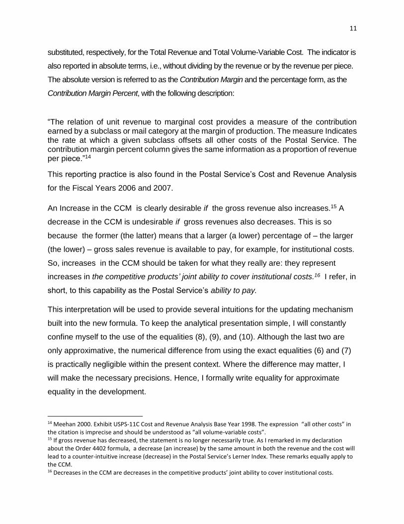
substituted, respectively, for the Total Revenue and Total Volume-Variable Cost. The indicator is
also reported in absolute terms, i.e., without dividing by the revenue or by the revenue per piece.
The absolute version is referred to as the Contribution Margin and the percentage form, as the
Contribution Margin Percent, with the following description:
“The relation of unit revenue to marginal cost provides a measure of the contribution earned by a subclass or mail category at the margin of production. The measure Indicates the rate at which a given subclass offsets all other costs of the Postal Service. The contribution margin percent column gives the same information as a proportion of revenue per piece.”14
This reporting practice is also found in the Postal Service’s Cost and Revenue Analysis
for the Fiscal Years 2006 and 2007.
An Increase in the CCM is clearly desirable if the gross revenue also increases.15 A
decrease in the CCM is undesirable if gross revenues also decreases. This is so
because the former (the latter) means that a larger (a lower) percentage of – the larger
(the lower) – gross sales revenue is available to pay, for example, for institutional costs.
So, increases in the CCM should be taken for what they really are: they represent
increases in the competitive products’ joint ability to cover institutional costs.16 I refer, in
short, to this capability as the Postal Service’s ability to pay.
This interpretation will be used to provide several intuitions for the updating mechanism
built into the new formula. To keep the analytical presentation simple, I will constantly
confine myself to the use of the equalities (8), (9), and (10). Although the last two are
only approximative, the numerical difference from using the exact equalities (6) and (7)
is practically negligible within the present context. Where the difference may matter, I
will make the necessary precisions. Hence, I formally write equality for approximate
equality in the development.
14 Meehan 2000. Exhibit USPS-11C Cost and Revenue Analysis Base Year 1998. The expression “all other costs” in the citation is imprecise and should be understood as “all volume-variable costs”. 15 If gross revenue has decreased, the statement is no longer necessarily true. As I remarked in my declaration about the Order 4402 formula, a decrease (an increase) by the same amount in both the revenue and the cost will lead to a counter-intuitive increase (decrease) in the Postal Service’s Lerner Index. These remarks equally apply to the CCM. 16 Decreases in the CCM are decreases in the competitive products’ joint ability to cover institutional costs.
12
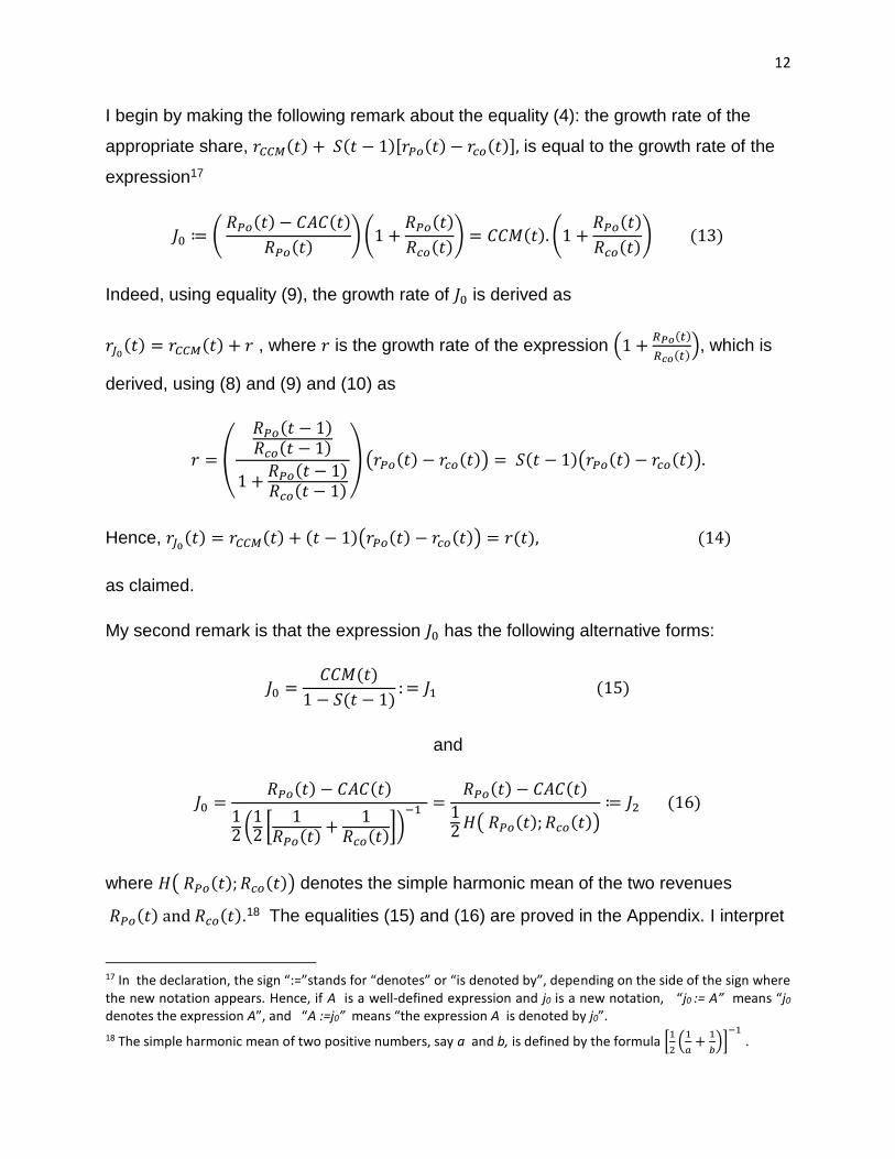
I begin by making the following remark about the equality (4): the growth rate of the
appropriate share, 𝑟𝐶𝐶𝑀(𝑡) + 𝑆(𝑡 − 1)[𝑟𝑃𝑜(𝑡) − 𝑟𝑐𝑜(𝑡)], is equal to the growth rate of the
expression17
𝐽0 ≔ ( 𝑅𝑃𝑜(𝑡) − 𝐶𝐴𝐶(𝑡)
𝑅𝑃𝑜(𝑡)) (1 +
𝑅𝑃𝑜(𝑡)
𝑅𝑐𝑜(𝑡)) = 𝐶𝐶𝑀(𝑡). (1 +
𝑅𝑃𝑜(𝑡)
𝑅𝑐𝑜(𝑡)) (13)
Indeed, using equality (9), the growth rate of 𝐽0 is derived as
𝑟𝐽0(𝑡) = 𝑟𝐶𝐶𝑀(𝑡) + 𝑟 , where 𝑟 is the growth rate of the expression (1 +
𝑅𝑃𝑜(𝑡)
𝑅𝑐𝑜(𝑡)), which is
derived, using (8) and (9) and (10) as
𝑟 = (
𝑅𝑃𝑜(𝑡 − 1)𝑅𝑐𝑜(𝑡 − 1)
1 +𝑅𝑃𝑜(𝑡 − 1)𝑅𝑐𝑜(𝑡 − 1)
) (𝑟𝑃𝑜(𝑡) − 𝑟𝑐𝑜(𝑡)) = 𝑆(𝑡 − 1)(𝑟𝑃𝑜(𝑡) − 𝑟𝑐𝑜(𝑡)).
Hence, 𝑟𝐽0(𝑡) = 𝑟𝐶𝐶𝑀(𝑡) + (𝑡 − 1)(𝑟𝑃𝑜(𝑡) − 𝑟𝑐𝑜(𝑡)) = 𝑟(𝑡), (14)
as claimed.
My second remark is that the expression 𝐽0 has the following alternative forms:
𝐽0 =𝐶𝐶𝑀(𝑡)
1 − 𝑆(𝑡 − 1): = 𝐽1 (15)
and
𝐽0 =𝑅𝑃𝑜(𝑡) − 𝐶𝐴𝐶(𝑡)
12 (
12 [
1𝑅𝑃𝑜(𝑡)
+1
𝑅𝑐𝑜(𝑡)])
−1 =𝑅𝑃𝑜(𝑡) − 𝐶𝐴𝐶(𝑡)
12 𝐻( 𝑅𝑃𝑜(𝑡); 𝑅𝑐𝑜(𝑡))
≔ 𝐽2 (16)
where 𝐻( 𝑅𝑃𝑜(𝑡); 𝑅𝑐𝑜(𝑡)) denotes the simple harmonic mean of the two revenues
𝑅𝑃𝑜(𝑡) and 𝑅𝑐𝑜(𝑡).18 The equalities (15) and (16) are proved in the Appendix. I interpret
17 In the declaration, the sign “:=”stands for “denotes” or “is denoted by”, depending on the side of the sign where the new notation appears. Hence, if A is a well-defined expression and j0 is a new notation, “j0 := A” means “j0
denotes the expression A”, and “A :=j0” means “the expression A is denoted by j0”.
18 The simple harmonic mean of two positive numbers, say a and b, is defined by the formula [1
2(
1
𝑎+
1
𝑏)]
−1
.
13
them by noting that 𝐽1 and 𝐽2 are ratios and a ratio of two positive numbers increases to
become a ratio of two other positive numbers if and only if the rate of change in the
numerator exceeds that of the denominator.19
Focusing on 𝐽1first, the relations (4) and (14) imply, therefore, that
the appropriate share for the next fiscal year is raised if and only if the Postal Service’s
ability to pay has increased fast enough over the current fiscal year, where “fast
enough” means faster than competitor’s revenue, the latter evaluated relatively to total
market revenue.20
Formally, the increase in the appropriate share occurs if and only if 𝑟𝐶𝐶𝑀(𝑡) > 𝑟1−𝑠(𝑡).
To interpret the expression 𝐽2, I first note that the harmonic mean of the two revenues,
𝐻( 𝑅𝑃𝑜(𝑡); 𝑅𝑐𝑜(𝑡)), could be replaced by other means, for example, the usual average,
i.e., the arithmetic mean, or the geometric mean, etc. I indicate in the appendix, how the
rate 𝑟(𝑡) slightly changes with the changing of the type of the mean used at the
denominator of 𝐽2. The simple harmonic means has the property that it is biased
towards the smallest of the two numbers, which, in this case, is the Postal Service’s
competitive revenue, i.e., 𝑅𝑃𝑜(𝑡). So, 𝐻( 𝑅𝑃𝑜(𝑡); 𝑅𝑐𝑜(𝑡)) measures the market’s average
revenue per firm, albeit with a greater weight implicitly given to the Postal Service’s
revenue than its competitors’. I refer to 𝐻( 𝑅𝑃𝑜(𝑡); 𝑅𝑐𝑜(𝑡)), simply as the industry
average revenue.
With these preliminaries, the interpretation of the expression 𝐽2 almost mirrors that of 𝐽1.
Specifically, the relations (4) and (14) imply, here also, that
the appropriate share for the next fiscal year is raised if and only if the Postal Service’s
ability to pay – in absolute form– has increased fast enough over the current fiscal year,
where “fast enough” means faster than the industry average revenue.
19 Indeed, if A and B are these two positive numbers and A changes to A+a, while B changes to B+b, such that
A+a>0 and B+b>0, then 𝐴+𝑎
𝐵+𝑏 >
𝐴
𝐵 is equivalent to
𝐴+𝑎
𝐴 >
𝐵+𝑏
𝐵, which, in turn, is equivalent to
𝐴+𝑎
𝐴− 1 >
𝐵+𝑏
𝐵−
1. 20 In other words, faster than competitor’s market share.
14
Formally, the increase in the appropriate share occurs if and only if 𝑟𝐶𝐶𝑀𝐴(𝑡) > 𝑟𝐻(𝑡),
where 𝑟𝐶𝐶𝑀𝐴(𝑡) denotes the rate of change in the (absolute) CCM, and 𝑟𝐻(𝑡) denotes
the rate of change in the industry average revenue.21
Returning to the related questions that were asked in the introduction,
2.2.2. Are there other implicit reasons than those presented by the Commission to
design the formula that need to be made explicit?
(i) The new formula models the joint ability of the Postal Service’s competitive
products to cover institutional costs –in short, the Postal Service’s ability to
pay– both in absolute and in relative terms.
(ii) It compares the changes in the Postal Service’s ability to pay to appropriate
referential baselines. The changes in the Postal Service’s absolute ability to
pay is compared to changes in the industry average revenue, which is also an
absolute measure. The changes in the Postal Service’s relative ability to pay
is compared to changes in the competitors’ share of total market revenue,
which is also a relative measure.
Since the apparent purpose of the new formula is to index the change in the
appropriate share to the change in the Postal Service’s ability to pay, its underlying
modeling strategy and the associated decision rule are, in my view, logically sound.
2.2.3. Does this reasoning provide enough ground for using the formula as a
decision-making tool suitable to its intended use?
To answer this question, I find it useful to revisit the contribution margin and the
contribution margin ratio. The CCM, just as the contribution margin, is a piece of
accounting information, which, together with other accounting and economic data,
helps companies– in the present case, the Postal Service – measure their operating
leverage. The contribution margin, in fact, indicates the amount from sales that is
available to cover fixed costs and contribute to profit. Likewise, the CCM (absolute and
relative) should indicate the amount from (respectively the percentage of ) sales that is
21 I note here that, by the relation (6) or (9), the ½ multiplying the harmonic mean does not affect its growth rate.
15
available to the Postal Service to cover its institutional costs and other financial needs.
The flexibility that it has, or ought to have, in allocating the CCM should be a factor to
consider by the Commission in deciding about the minimum share. These
considerations raise the question stated in the introduction regarding the principles
guiding the Commission’s minimum-share updating policy. I believe that it is worth
repeating and emphasizing this question: Should any relative increase (or any
relative decrease) in the Postal Service’s ability to pay be automatically construed as an
increase (respectively, a decrease) in its obligation to pay?
The answer to the section’s title-question is, in my view, contingent on the answer to
the last question. The new formula is suitable to be used as an updating rule of the
appropriate share only if the Commission’s guiding principle is that all relative increases
(or decreases) in the Postal Service’s ability to pay are to be considered in full as
increases (respectively, decreases) in its obligation to pay. However, the precept that
the Commission is seeking to determine the appropriate share as a minimum, should
lead it to take into consideration in its decision to increase or lower the appropriate
share, the existence of other financial needs that the Postal Service’s contribution
margin could cover. The complexity of the judgments required by this consideration is
less amenable to a simple mathematical updating rule as the one implied by the new
formula.
2.3. Stability of the New Recursive Equation
2.3.1. Overview
To study the stability of the new formula, Equation (4) will be written in the cumulative
product form as
𝐴𝑆𝑡+1 = 𝐴𝑆0 ∏ {1 + 𝑟(𝑗)}𝑗=𝑡𝑗=0 (17)
where the initial time is conveniently relabeled as zero and
𝑟(𝑗) ≔ 𝑟𝐶𝐶𝑀(𝑗) + 𝑆(𝑗 − 1)[𝑟𝑃𝑜(𝑗) − 𝑟𝑐𝑜(𝑗)] (18)
16
This section has three objectives. The first is to define a popular notion of stability –
Lyapunov stability – and, more importantly, to show that in the context of the new
formula, some of the conditions that insure this property may be undesirable.
Specifically, I first remark the fact that (i) the zero minimum share is an equilibrium
share and (ii) constant erosion of the Postal Service’s ability to pay – relatively to the
reference baselines – would guaranty the Lyapunov stability of this equilibrium share,
which is not necessarily an attractive scenario.22
However, in regard of the prospect that the Commission is seeking to compute an ex-
ante minimum share, i.e., a share that is a minimum before its enforcement as a
required minimum, Lyapunov stability is – or may be – a desirable property, because it
insures that if the initial share is close enough to zero, all subsequence shares will be
wandering in the neighborhood of zero. In fact, in the present case, as I will soon show,
Lyapunov stability of the equilibrium share has the necessary consequence that the
computed shares will, in the long run become arbitrarily close to one another, i.e.,
converge to a limit that remains in the neighborhood of zero, provided that the initial
share is set close enough to zero.
The second objective is to provide alternative sufficient conditions – conditions that are
different from Lyapunov stability, but are by no means necessary – for the convergence
of the computed shares to a limit when the time tends to infinity. The last objective is to
discuss questions related to the possibility of unpredictable erratic trends in the
computed shares.
2.3.2. Equilibrium Share, Lyapunov Stability, and Asymptotic Stability
“Stability” is a word primarily used in system theory, an interdisciplinary study of
systems, where the word “system” designates any “complex of interacting elements”.23
In the present context, the new formula can be thought off as a mathematical
description of a dynamic – or time-evolving – system.
22 In fact, they insure the convergence of the shares to zero. 23 Von Bertalanffy, L. 1968. General System theory: Foundations, Development, Applications, New York: George Braziller, Page 55.
17
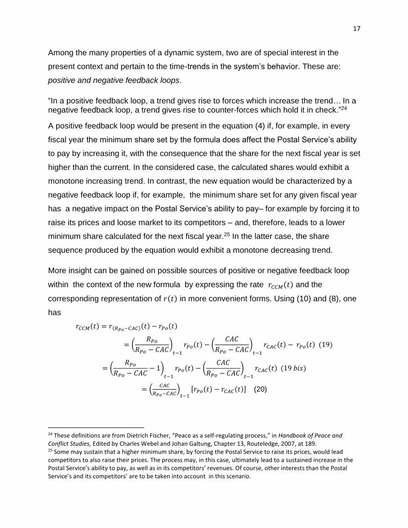
Among the many properties of a dynamic system, two are of special interest in the
present context and pertain to the time-trends in the system’s behavior. These are:
positive and negative feedback loops.
“In a positive feedback loop, a trend gives rise to forces which increase the trend… In a negative feedback loop, a trend gives rise to counter-forces which hold it in check.”24
A positive feedback loop would be present in the equation (4) if, for example, in every
fiscal year the minimum share set by the formula does affect the Postal Service’s ability
to pay by increasing it, with the consequence that the share for the next fiscal year is set
higher than the current. In the considered case, the calculated shares would exhibit a
monotone increasing trend. In contrast, the new equation would be characterized by a
negative feedback loop if, for example, the minimum share set for any given fiscal year
has a negative impact on the Postal Service’s ability to pay– for example by forcing it to
raise its prices and loose market to its competitors – and, therefore, leads to a lower
minimum share calculated for the next fiscal year.25 In the latter case, the share
sequence produced by the equation would exhibit a monotone decreasing trend.
More insight can be gained on possible sources of positive or negative feedback loop
within the context of the new formula by expressing the rate 𝑟𝐶𝐶𝑀(𝑡) and the
corresponding representation of 𝑟(𝑡) in more convenient forms. Using (10) and (8), one
has
𝑟𝐶𝐶𝑀(𝑡) = 𝑟(𝑅𝑃𝑜−𝐶𝐴𝐶)(𝑡) − 𝑟𝑃𝑜(𝑡)
= (𝑅𝑃𝑜
𝑅𝑃𝑜 − 𝐶𝐴𝐶)
𝑡−1
𝑟𝑃𝑜(𝑡) − (𝐶𝐴𝐶
𝑅𝑃𝑜 − 𝐶𝐴𝐶)
𝑡−1
𝑟𝐶𝐴𝐶(𝑡) − 𝑟𝑃𝑜(𝑡) (19)
= (𝑅𝑃𝑜
𝑅𝑃𝑜 − 𝐶𝐴𝐶− 1)
𝑡−1
𝑟𝑃𝑜(𝑡) − (𝐶𝐴𝐶
𝑅𝑃𝑜 − 𝐶𝐴𝐶)
𝑡−1
𝑟𝐶𝐴𝐶(𝑡) (19 𝑏𝑖𝑠)
= (𝐶𝐴𝐶
𝑅𝑃𝑜−𝐶𝐴𝐶)
𝑡−1[𝑟𝑃𝑜(𝑡) − 𝑟𝐶𝐴𝐶(𝑡)] (20)
24 These definitions are from Dietrich Fischer, “Peace as a self-regulating process,” in Handbook of Peace and Conflict Studies, Edited by Charles Webel and Johan Galtung, Chapter 13, Routeledge, 2007, at 189. 25 Some may sustain that a higher minimum share, by forcing the Postal Service to raise its prices, would lead competitors to also raise their prices. The process may, in this case, ultimately lead to a sustained increase in the Postal Service’s ability to pay, as well as in its competitors’ revenues. Of course, other interests than the Postal Service’s and its competitors’ are to be taken into account in this scenario.
18
where (𝐶𝐴𝐶
𝑅𝑃𝑜−𝐶𝐴𝐶)
𝑡−1 is written as a shorthand for (
𝐶𝐴𝐶(𝑡−1)
𝑅𝑃𝑜(𝑡−1)−𝐶𝐴𝐶(𝑡−1)). The rate of change 𝑟(𝑡)
can, consequently, be written as
𝑟(𝑡)=(𝐶𝐴𝐶
𝑅𝑃𝑜−𝐶𝐴𝐶)
𝑡−1[𝑟𝑃𝑜(𝑡) − 𝑟𝐶𝐴𝐶(𝑡)] + 𝑆(𝑡 − 1)[𝑟𝑃𝑜(𝑡) − 𝑟𝑐𝑜(𝑡)] (21)
or
𝑟(𝑡)=(𝐶𝐴𝐶
𝑅𝑃𝑜−𝐶𝐴𝐶)
𝑡−1𝑟
(𝑅𝑃𝑜𝐶𝐴𝐶
)(𝑡) + 𝑆(𝑡 − 1)𝑟
(𝑅𝑃𝑜𝑅𝑐𝑜
)(𝑡) (22)26
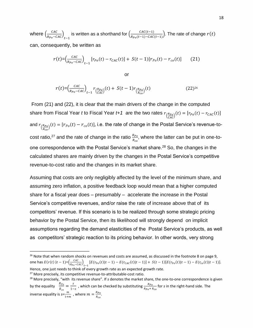
From (21) and (22), it is clear that the main drivers of the change in the computed
share from Fiscal Year t to Fiscal Year t+1 are the two rates 𝑟(
𝑅𝑃𝑜𝐶𝐴𝐶
)(𝑡) = [𝑟𝑃𝑜(𝑡) − 𝑟𝐶𝐴𝐶(𝑡)]
and 𝑟(
𝑅𝑃𝑜𝑅𝑐𝑜
)(𝑡) = [𝑟𝑃𝑜(𝑡) − 𝑟𝑐𝑜(𝑡)], i.e. the rate of change in the Postal Service’s revenue-to-
cost ratio,27 and the rate of change in the ratio 𝑅𝑃𝑜
𝑅𝑐𝑜, where the latter can be put in one-to-
one correspondence with the Postal Service’s market share.28 So, the changes in the
calculated shares are mainly driven by the changes in the Postal Service’s competitive
revenue-to-cost ratio and the changes in its market share.
Assuming that costs are only negligibly affected by the level of the minimum share, and
assuming zero inflation, a positive feedback loop would mean that a higher computed
share for a fiscal year does – presumably – accelerate the increase in the Postal
Service’s competitive revenues, and/or raise the rate of increase above that of its
competitors’ revenue. If this scenario is to be realized through some strategic pricing
behavior by the Postal Service, then its likelihood will strongly depend on implicit
assumptions regarding the demand elasticities of the Postal Service’s products, as well
as competitors’ strategic reaction to its pricing behavior. In other words, very strong
26 Note that when random shocks on revenues and costs are assumed, as discussed in the footnote 8 on page 9,
one has 𝐸(𝑟(𝑡) |𝑡 − 1)=(𝐶𝐴𝐶
𝑅𝑃𝑜−𝐶𝐴𝐶)
𝑡−1[𝐸(𝑟𝑃𝑜(𝑡)|𝑡 − 1) − 𝐸(𝑟𝐶𝐴𝐶(𝑡)|𝑡 − 1)] + 𝑆(𝑡 − 1)[𝐸(𝑟𝑃𝑜(𝑡)|𝑡 − 1) − 𝐸(𝑟𝑐𝑜(𝑡)|𝑡 − 1)].
Hence, one just needs to think of every growth rate as an expected growth rate. 27 More precisely, its competitive revenue-to-attributable-cost ratio. 28 More precisely, “with its revenue share”. If s denotes the market share, the one-to-one correspondence is given
by the equality 𝑅𝑃𝑜
𝑅𝑐𝑜=
𝑠
1−𝑠 , which can be checked by substituting
𝑅𝑃𝑜
𝑅𝑃𝑜+ 𝑅𝑐𝑜 for s in the right-hand side. The
inverse equality is s=𝑚
1+𝑚 , where 𝑚 =
𝑅𝑃𝑜
𝑅𝑐𝑜.
19
assumptions on the dynamic market game between the incumbent firms are needed to
sustain the scenario. In the case of a negative feedback loop, the higher minimum
share does – presumably – cause a deceleration of the Postal Service’s competitive
revenues, relatively to its costs and/or relatively to the rate of change in competitors’
revenue. Here also, to sustain the scenario, one would need to make highly
questionable assumptions on the channel through which the minimum share affects
the market game. These remarks are not to say that the minimum share does not affect
the market game. It simply questions any potential claim that it does so in a very
specific way.
The question regarding the exhibition of possible feedback loops is closely related to
the general question of the stability properties of the formula. There are diverse types of
stability with corresponding mathematical definitions. Some of them are classic in
system theory. I focus here on two notions of stability, using the notations that I have
adopted in the declaration.
I begin by remarking that the system described by the new equation is non-
autonomous. To explain this notion, I note that Equation (4) can, more generally, be
written as
𝐴𝑆𝑡+1 = 𝑓(𝐴𝑆𝑡, 𝑡) (23)
where 𝑓(𝐴𝑆𝑡, 𝑡) denotes the expression 𝐴𝑆𝑡{1 + 𝑟𝐶𝐶𝑀(𝑡) + 𝑆(𝑡 − 1)[𝑟𝑃𝑜(𝑡) − 𝑟𝑐𝑜(𝑡)]}.
In other words, some function, 𝑓(. , 𝑡), which depends on time, transforms the share 𝐴𝑆𝑡,
set for the fiscal year t, into the share 𝐴𝑆𝑡+1 for the fiscal year t+1. The function, in the
present context, depends on time through the growth rates 𝑟(𝑡) = 𝑟𝐶𝐶𝑀(𝑡) + 𝑆(𝑡 −
1)[𝑟𝑃𝑜(𝑡) − 𝑟𝑐𝑜(𝑡). If this growth rate is constant over time, 𝑟(𝑡) = 𝑟, 𝑡 = 1,2,3, 𝑒𝑡𝑐,
then the system is called autonomous, in which case, the equation (23) becomes
𝐴𝑆𝑡+1 = 𝑓(𝐴𝑆𝑡) (24)
Next, I note that the notions of stability, which will be defined below, applies to an
equilibrium point – in our case, an equilibrium share – implied by the formula. Hence,
the proper terminology is the stability of an equilibrium share, rather than the stability of
20
the formula, even though I will be using these two expressions interchangeably. I now
define the notion of equilibrium share.
Definition: Equilibrium Share
For the non-autonomous system 𝐴𝑆𝑡+1 = 𝑓(𝐴𝑆𝑡, 𝑡), the share 𝐴𝑆 is an equilibrium share
if and only if 𝐴𝑆 = 𝑓(𝐴𝑆, 𝑡) for all t, t=0,1,2, etc.29
By simply substituting the value 0 for 𝐴𝑆𝑡 in equation (4) it is clear that 𝐴𝑆 = 0 is an
equilibrium share in the equation, i.e., 0 = 𝑓(0, 𝑡) for all t. In fact, as one can verify, it
also is the only equilibrium share.
I define, next, the notion of stability. In words and as already stated above, Lyapunov
stability of an equilibrium share is about the wandering of the computed shares towards
the equilibrium share. A related notion of stability is asymptotic stability. Asymptotic
stability is about the properties of the computed shares to gradually approach the
equilibrium share as time evolves. More precisely,
2.3.3. Stability30
The equilibrium point 𝐴𝑆 = 0
is Lyapunov-stable (stable in the sense of Lyapunov) if for each 휀 > 0, and any time
𝑡 = 𝑡0, there is 𝛿 = 𝛿(휀, 𝑡0) > 0 (that may depend on 휀, and 𝑡0) such that 𝐴𝑆𝑡0<
𝛿(휀, 𝑡0) implies 𝐴𝑆𝑡 < 휀 for all t following 𝑡0. 31
is asymptotically stable if it is Lyapunov stable and there is a positive constant 𝑘(휀) >
0 (that may depend on 휀), such that 𝐴𝑆𝑡 converges to the equilibrium share 0 as t tends
to infinity, provided that the inequality 𝐴𝑆𝑡0< 𝑘(휀) holds.32
29 So, once the recursion reaches an equilibrium share, it keeps reproducing that share forever. 30 See, for example, Slotine J-J. E. , and W. Li, Applied Nonlinear Control, Prentice Hall, 1991, at 48-50. 31 The last two inequalities should be stated with 𝐴𝑆𝑡0
and 𝐴𝑆𝑡 taken in absolute values. In our case, however, the
shares are non-negative numbers, hence equal to their absolute values. 32 In other words, if the share at some time 𝑡0 is set close enough to zero (that is what condition 𝐴𝑆𝑡0
< 𝑘(휀)
means), then the subsequent shares converge to zero as if they fall under the spell of a force which direct them progressively towards zero.
21
In the equation (4), the equilibrium point 𝐴𝑆 = 0 is clearly Lyapunov-stable if the growth
rate 𝑟(𝑡) = 𝑟𝐶𝐶𝑀(𝑡) + 𝑆(𝑡 − 1)[𝑟𝑃𝑜(𝑡) − 𝑟𝑐𝑜(𝑡) is negative for all fiscal years.33 This
sufficient condition is undesirable, however, since it means that the Postal Service’s
ability to pay degrades – in relative terms – every fiscal year.34 The Commission should
not have any particular preference for the zero share, compared to other non-zero
shares. It may be important, in this regard, to recall the statutory provisions regarding
the review of the appropriate share by the Commission:
…the Postal Regulatory Commission shall conduct a review to determine whether the institutional costs contribution requirement under subsection (a)(3) should be retained in its current form, modified, or eliminated. 39 U.S.C. § 3633 (b).
The elimination of the institutional costs contribution requirement under subsection
(a)(3) is effectively equivalent to setting the appropriate share permanently to zero. This
is, however, just one of the options that the Commission is asked to consider.
A pattern of strictly decreasing rates 𝑟(𝑡) is, however, not a necessary condition for
Lyapunov stability and the fact that it can be realized by a problematic scenario does
not make this type of stability, an absolutely undesirable property. In fact, in the specific
case under consideration, Lyapunov stability has the consequence that it implies the
convergence of the shares to some limit share.
To show this, I assume that the zero-share is Lyapunov stable. This means that I can
choose 𝛿(휀, 𝑡0) such that, once the inequality 𝐴𝑆𝑡0< 𝛿(휀, 𝑡0) is satisfied, all the
subsequent shares – subsequent to 𝑡0– satisfy the inequality
𝐴𝑆𝑡 < 휀 or, using equation (17), 𝐴𝑆𝑡 = 𝐴𝑆𝑡0∏ {1 + 𝑟(𝑗)}𝑗=𝑡−1
𝑗=0 < 휀
The last inequality implies, however, by letting t grow indefinitely, that the infinite
product 𝐴𝑆𝑡0∏ {1 + 𝑟(𝑗)}∞
𝑗=0 is finite in magnitude (because it is less than or equal to
33 Indeed, choosing 𝛿(휀, 𝑡0) = 휀, all the 𝐴𝑆𝑡, for the t following 𝑡0, will be smaller than 휀 . This is so, because they are decreasing in magnitude (negative growth rate) and the first, 𝐴𝑆𝑡0
, is less than 𝛿(휀, 𝑡0) = 휀. 34 This is an example in which stability may not be a desirable property, for a system.
22
휀)35 . Either one of the 𝐴𝑆𝑡 is zero (in which case all the following are), or none is and
the shares converge to a limit that is not necessarily null, a topic that I discuss below.
To summarize, Lyapunov stability implies the convergence of the computed shares, but
not necessarily to zero (nor to 1). In fact, the mere convergence of the share does not
mean or imply asymptotic stability, which requires the limit to be equal to the zero-
share.
It should be apparent from the above development that in the present context,
Lyapunov stability cannot be unequivocally proved or disproved, because any proof
would have to rely on unverifiable, hence questionable, assumptions on the dynamics of
the Postal Service’s ability to pay.
I now turn to the long run properties of the formula.
2.3.4. What to Expect in the Long-Run
By definition, the right-hand size of (17) converges to a non-zero limit if, beyond some
time point, say 𝜏 , none of the factors vanishes and the partial products
𝑝𝑛 ≔ (1 + 𝑟(𝜏 + 1))(1 + 𝑟(𝜏 + 2))(1 + 𝑟(𝜏 + 3)) … . (1 + 𝑟(𝜏 + 𝑛))
converge, as n increases, to a limit that is finite and different from 0.36 A necessary
condition for this to occur is that the growth rate 𝑟(𝑡) tends to zero as t tends to
infinity.37 As it will be become apparent below, this last condition essentially means that
product-specific price-to-unit-attributable-cost and product-specific price ratios between
the Postal Service and its competitors, eventually reach steady states. A simple
application of a result by Knopp (1954)38 leads to the seemingly obvious conclusion that
35 If a sequence of real numbers is convergent and has all its terms (starting with some rank) strictly less than some
positive 휀, then the limit is less than or equal to 휀. The “equal to” part of the sentence comes from the fact that the limit of the sequence has to be a limit point (or an accumulation point) of the open interval (−∞, 휀). Since the
boundary point, 휀, is one of these limit points, it could possibly be the limit of the sequence. 36 Cf. Konrad Knopp, Theory and Application of Infinite Series, Chapter VII “Infinite Products”, Blackie and Son Limited, at 218. 37 Since both 𝑝𝑛 and 𝑝𝑛−1 converge to the same non-zero limit, their ratio
𝑝𝑛
𝑝𝑛−1= 1 + 𝑟(𝑛) converges to 1. In
other words, a necessary condition for convergence is that the growth rate 𝑟(𝑡) tends to zero as t tends to infinity. Knopp. Op. Cit. at 219. 38 Knopp Op.cit. Proof of Theorem 5. Page 222.
23
the computed shares converge to a limit if and only if they eventually become arbitrarily
close to one another.39
There are various sufficient conditions for the convergence.40 One is that the infinite
sum ∑ 𝑟(𝜏)∞𝜏=1 be absolutely convergent, i.e., ∑ |𝑟(𝜏)|∞
𝜏=1 be a convergent series.41
Another is that both ∑ 𝑟(𝜏)∞𝜏=1 and ∑ 𝑟(𝜏)2∞
𝜏=1 be convergent series. Intuitively, the last
conditions have the following meaning: if one measures the size of the infinite
sequence of change rates, (𝑟(1), 𝑟(2), 𝑟(3) … ) by the limit of the sum ∑ 𝑟(𝜏)𝑡𝜏=1 , or of
the sum ∑ 𝑟(𝜏)2𝑡𝜏=1 , then the sufficient condition is that these two sizes be finite in
magnitude.
Since the limit – in case of convergence – depends on the initial share, it can, at least in
principle, be controlled by properly setting this initial share. In that sense, convergence
may be viewed as a desirable property. However, conditions that insure this property,
such as the ones provided above, are, here also, impossible to verify directly from the
formula, as they concern the entire sequence (𝑟(1), 𝑟(2), 𝑟(3) … ) of change rates,
hence, the time path of the Postal Service’s ability to pay.42
If the underlying concern for worrying about the stability of the formula is the possibility
that it generates patterns of shares with abrupt and unpredictable changes, then more
intuitions on the likelihood of these patterns can be gained from examining how the
relative rates of change in the Postal Service’s ability to pay relates to the rates of
39 More precisely, the computed shares converge to a limit if and only if, given 휀 > 0 , along with some initial time
𝑡0 and a positive integer 𝑘 ( all three arbitrary), after a suitable time following 𝑡0, all the computed share satisfy
the inequality |𝐴𝑆𝑡+𝑘−𝐴𝑆𝑡
𝐴𝑆𝑡| < 휀 , i.e. the shares become arbitrarily close to one another.
40 Cf, Knopp, Op. Cit. pp 222-226. 41 Intuitively, if the size of the series of change rates in the computed shares, 𝑟(1), 𝑟(2), … is measured by the limit
when t tends to infinity of the sum ∑ |𝑟(𝜏)|𝑡𝜏=1 then the required condition is that this size be finite in magnitude.
42 One may be tempted to take the logarithms of both sides of 𝐴𝑆𝑡 = 𝐴𝑆𝑡0∏ {1 + 𝑟(𝑗)}𝑗=𝑡−1
𝑗=0 and examine the
series ∑ 𝑙𝑛{1 + 𝑟(𝑗)}∞𝑗=0 for convergence, which is not an easier exercise than its the product-form counterpart. In
fact, the convergence problem becomes very difficult when 𝑟(𝑗) is considered random, because in that case, one has to state and discuss the realistic satisfaction of general conditions of convergence of a random series, such as those in Wu, W. B. and M. Woodroofe , “Martingale Approximations for Sums of Stationary Processes,” The Annals of Probability, Vol. 32, No. 2 (Apr., 2004), pp. 1674-1690.
24
change in product-specific price-to-costs – more precisely, price to per-piece
attributable cost– , and price ratios, relatively to competitors’ prices. The only
assumption needed here for this kind of analysis is that the Postal Service (PS) and its
competitors produce (pairwise) comparable products and the total number of such pairs
of products on the market is N.43
To better appreciate the conclusions that will follow below from the analytic
development, it is important, I believe, to say a word about the overarching perspective.
As already stated (on page 14), the reasoning underlying the new formula is to index
the change in the appropriate share to the change in the Postal Service’s ability to pay.
This can be alternatively be expressed as the equality
[change rate in the appropriate share =change rate in the Postal Service’s ability to
pay].44
From this fact follows the consequence that the formula-generated sequence of
appropriate shares and the sequence, 𝑟(𝑡), 𝑡 = 1,2, 𝑒𝑡𝑐., of the relative growth rates in
the Postal Service’s ability to pay, have exactly the same time-trend.45 Hence, to predict
the time-trends in the first, one needs to understand what is at play in the second,
especially at product-specific level. The question to ask is, therefore, what drives the
trends in the Postal Services ability to pay at the micro-level, i.e., at product-specific
level?
The rate of change of the share in the fiscal year t, 𝑟(𝑡), has already been shown to
satisfy the equalities (Relation (21) and (22))
𝑟(𝑡)=(𝐶𝐴𝐶
𝑅𝑃𝑜−𝐶𝐴𝐶)
𝑡−1[𝑟𝑃𝑜(𝑡) − 𝑟𝐶𝐴𝐶(𝑡)] + 𝑆(𝑡 − 1)[𝑟𝑃𝑜(𝑡) − 𝑟𝑐𝑜(𝑡)]
43 In a comparative perspective, the assumption is necessary. It is implicit and, sometime, explicit in theoretical frameworks that compare a firm’s pricing behavior to its competitors’. For example, in Sappington, D. E. M., and J. G. Sidak, “Incentives for Anticompetitive Behavior by Public Enterprises,” Review of Industrial Organization 22: 183–206, 2003, the authors make similar assumptions about the products that are traded on the market. At 187. 44 Or,
𝐴𝑆𝑡+1−𝐴𝑆𝑡
𝐴𝑆𝑡= 𝑟(𝑡).
45 An analogy may be useful here: if, for example, some given price is strictly indexed to inflation, then the trend in the price is nothing more or less than the trend in inflation.
25
or
𝑟(𝑡)=(𝐶𝐴𝐶
𝑅𝑃𝑜−𝐶𝐴𝐶)
𝑡−1𝑟
(𝑅𝑃𝑜𝐶𝐴𝐶
)(𝑡) + 𝑆(𝑡 − 1)𝑟
(𝑅𝑃𝑜𝑅𝑐𝑜
)(𝑡)
Hence, given the values of the year t-1 factors, (𝐶𝐴𝐶
𝑅𝑃𝑜−𝐶𝐴𝐶)
𝑡−1and 𝑆(𝑡 − 1),46 the rates 𝑟(𝑡)
is a combination of the two rates 𝑟(
𝑅𝑃𝑜𝐶𝐴𝐶
)(𝑡) and 𝑟
(𝑅𝑃𝑜𝑅𝑐𝑜
)(𝑡). Switching the focus to the two
underlying ratio, 𝑅𝑃𝑜
𝐶𝐴𝐶 and
𝑅𝑃𝑜
𝑅𝑐𝑜 , I show in the appendix the equalities
𝑅𝑃𝑜(𝑡)
𝐶𝐴𝐶(𝑡)= ∑ (
𝑝𝑃𝑜,𝑖
(𝑡)
𝑎𝑖(𝑡))
𝑖=𝑁
𝑖=1
(𝐶𝐴𝐶𝑖(𝑡)
∑ 𝐶𝐴𝐶𝑖(𝑡)𝑖=𝑁𝑖=1
) (25)
= ∑ ( 𝑝𝑃𝑜,𝑖(𝑡)
𝑎𝑖(𝑡))𝑖=𝑁
𝑖=1 𝑤𝑎,𝑖(𝑡), where 𝑤𝑎,𝑖(𝑡): = (𝑅𝑐𝑜,𝑖(𝑡)
∑ 𝑅𝑐𝑜,𝑖(𝑡)𝑖=𝑁𝑖=1
), (26)
Where 𝑎𝑖(𝑡) denotes, I recall, the unit attributable cost.
Hence, the revenue-to-attributable-cost ratio, 𝑅𝑃𝑜(𝑡)
𝐶𝐴𝐶(𝑡), is expressible as a weighted
average of the product-specific price-to-cost ratios, ( 𝑝𝑃𝑜,𝑖(𝑡)
𝑎𝑖(𝑡)), with the corresponding
weights 𝑤𝑎,𝑖(𝑡): = (𝐶𝐴𝐶𝑖(𝑡)
∑ 𝐶𝐴𝐶𝑖(𝑡)𝑖=𝑁𝑖=1
) . Since the terms ( 𝑝𝑃𝑜,𝑖(𝑡)
𝑎𝑖(𝑡)) 𝑤𝑎,𝑖(𝑡) are all non-negative, the
growth rate of the sum is a weighted average –with weights that are different from
𝑤𝑎,𝑖(𝑡) − of the growth rates of these terms. 47 As an average, it is certainly not larger
than the maximum of the growth rates of the terms. One may then ask the following
question :
Question 1
What time-path are the product-specific price-to-cost ratios likely to follow over a given
period of time, and what time-path are their corresponding cost weights, 𝑤𝑎,𝑖(𝑡) =𝐶𝐴𝐶𝑖(𝑡)
∑ 𝐶𝐴𝐶𝑖(𝑡)𝑖=𝑁𝑖=1
, likely to follow over the same period of time? Are these paths likely to be
moderate or, instead, chaotic, explosive, unpredictable?
46 The ratio (
𝐶𝐴𝐶
𝑅𝑃𝑜−𝐶𝐴𝐶)
𝑡−1 can also be written as (
1−𝐶𝐶𝑀
𝐶𝐶𝑀)
𝑡−1 . The other factor, 𝑆(𝑡 − 1) is, I recall, the Postal
Service’s market share in the fiscal year t-1. 47 The growth rate of (
𝑝𝑃𝑜,𝑖(𝑡)
𝑎𝑖(𝑡)) 𝑤𝑎,𝑖(𝑡) is the sum of the growth rates of the factors.
26
The second ratio, 𝑅𝑃𝑜
𝑅𝑐𝑜, can similarly be decomposed as the first to obtain
𝑅𝑃𝑜
𝑅𝑐𝑜= ∑ (
𝑝𝑃𝑜,𝑖(𝑡)
𝑝𝑐𝑜,𝑖(𝑡)
)
𝑖=𝑁
𝑖=1
𝑤𝑐𝑜,𝑖(𝑡), where 𝑤𝑐𝑜,𝑖(𝑡): = (𝑅𝑃𝑜,𝑖(𝑡)
∑ 𝑅𝑃𝑜,𝑖(𝑡)𝑖=𝑁𝑖=1
) (27)
In other words, the ratio 𝑅𝑃𝑜
𝑅𝑐𝑜 is the average of the product-specific price ratios,
𝑝𝑃𝑜,𝑖(𝑡)
𝑝𝑐𝑜,𝑖(𝑡),
weighted by the competitors’ revenue-weights 𝑤𝑐𝑜,𝑖(𝑡): = (𝑅𝑃𝑜,𝑖(𝑡)
∑ 𝑅𝑃𝑜,𝑖(𝑡)𝑖=𝑁𝑖=1
). The second
question of interest is, therefore:
Question 2
What time-path are the product-specific price-ratios, 𝑝𝑃𝑜,𝑖(𝑡)
𝑝𝑐𝑜,𝑖(𝑡), likely to follow over a given
period of time, and what time-path are their corresponding revenue weights, 𝑤𝑐𝑜,𝑖(𝑡): =
(𝑅𝑃𝑜,𝑖(𝑡)
∑ 𝑅𝑃𝑜,𝑖(𝑡)𝑖=𝑁𝑖=1
), likely to follow over the same period of time? Are these paths likely to be
moderate or, instead, chaotic, explosive, unpredictable?
Answers to and Implications of Questions 1 and 2
If the variables in questions 1 and 2 are expected to remain on moderate paths over
the period of interest, so will be the shares computed by the formula. If they are
expected to be rather volatile, so will again be the shares computed by the formula.48
From a predictive perspective, the stability of the formula (the word is used in this
sentence to refer to an unpredictable, erratic behavior) depends, not on market
equilibrium outcomes – price-to-unit-cost ratios and price ratios relative to competitors,
or cost and revenue structures –, if any, as they can be predicted by alternative
economic theories or models, but rather on whether these predicted outcomes are
expected to be changing erratically from year to year. Hence, a theory that assumes or
predicts that the equilibrium outcomes, if any, do not change drastically over time does,
also predicts, in fact, that the formula will be stable, in the sense that it will produce
shares with moderate time paths. This is so because the formula is only about the rates
of change over time in these outcomes. It is not about the levels of these outcomes.
48 In fact, the formation of expectations about the time path of the Postal Service’s ability to pay is even more difficult if one considers the possibility that this path is affected by possible feedback loops.
27
The ratio nature of these outcomes is also very important. In fact, if one asks
What does the formula produce if all revenues, 𝑅𝑃𝑜(𝑡) and 𝑅𝑐𝑜(𝑡) , and the attributable cost 𝐶𝐴𝐶(𝑡) grow over time at a same rate? The answer is readily provided by the equality
𝑟(𝑡)=(𝐶𝐴𝐶
𝑅𝑃𝑜−𝐶𝐴𝐶)
𝑡−1[𝑟𝑃𝑜(𝑡) − 𝑟𝐶𝐴𝐶(𝑡)] + 𝑆(𝑡 − 1)[𝑟𝑃𝑜(𝑡) − 𝑟𝑐𝑜(𝑡)].
If (𝑟𝑃𝑜(𝑡) = 𝑟𝐶𝐴𝐶(𝑡) = 𝑟𝑐𝑜(𝑡)), then 𝑟(𝑡) = 0, in other words, the computed share remains
unchanged over time under the stated assumption, a fortiori if that common growth rate
is constant over time (steady state equilibrium). It should not come as a surprise,
therefore, that, provided the two revenues, 𝑅𝑃𝑜(𝑡) and 𝑅𝑐𝑜(𝑡), and the attributable cost,
𝐶𝐴𝐶(𝑡), all change at the same annual rate, say 𝛾(𝑡), and regardless of how
fluctuating the rate 𝛾(𝑡) may be from one year to the next, the computed appropriate
share will remain unchanged over the relevant period of time. This is so, once again,
because only the growth rates of the ratios 𝑅𝑃𝑜(𝑡)/𝑅𝑐𝑜(𝑡), and 𝐶𝐶𝐴(𝑡)/𝑅𝑃𝑜(𝑡) drive the
updating mechanism built into the formula. Not the individual growth rates of 𝑅𝑃𝑜(𝑡),
𝑅𝑐𝑜(𝑡), and 𝐶𝐴𝐶(𝑡).
To conclude about the topic of stability, I will state the following: the Lyapunov-stability
of the equilibrium share may be a desirable property, because it implies the long-term
convergence of the computed shares to a limit, which depends on the magnitude of the
initial share. However, as stated above, as it pertains to the Commission’s formula,
Lyapunov-stability, and a fortiori, asymptotic stability, cannot be proved or disproved
without making questionable assumptions on the dynamics of the Postal Service’s
ability to pay.
As for the odds of erratic trends in the time paths of the computed shares, they
ultimately depend on whether the fundamental equilibria, if any, associated with the
underlying market games, which produces the observable trends in prices and volumes,
both at product and aggregate levels, have moderate time evolutions or not.
28
Because, in the present case, any formal proof of the discussed types of stability – or
of the lack of stability – cannot avoid relying on unverifiable assumptions on the likely
time path of the Postal Service’s ability to pay, an alternative – and more modest – goal
is to provide in the appendix, a piece of simulation-based information, with the hope
that it will help gain some insights about the time paths of the calculated shares over
relatively short horizons. The discussion of this simulation strategy is the purpose of the
following section.
2.3.5. Scenarios for a Five-Year Period
Equation (4) is reproduced here for convenience:
𝐴𝑆𝑡+1 = 𝐴𝑆0 ∏ {1 + 𝑟(𝑗)}𝑗=𝑡𝑗=0 ,49 (17)
The time paths of the minimum shares produced by the new formula for the next five
years can be simulated based on values assigned to the growth rate, (𝑟𝐶𝐶𝑀(𝑡) + 𝑆(𝑡 −
1)[𝑟𝑃𝑜(𝑡) − 𝑟𝑐𝑜(𝑡)]) . The historically highest rate computed from the data provided along
with Order No. 4742, occurred over the time span FY2016 to FY2017 and is equal to
+19.5%. In the setting of the new formula, this corresponds to the largest annual relative
increase in the Postal Service’s ability to pay over the period 2007-2017. The largest
relative decrease in its ability to pay was -8.1% and did occur over the time span
FY2016 to FY2017. Using these extreme rates of change, conservative paths can be
determined for the appropriate share over the next 5-year period. There are 32 different
paths that can be derived from this assumption of binary annual changes and they are
described in Table 1 in the appendix. In the table, the “plus” sign denotes an increase
while the “minus” sign, a decrease. Each of these paths takes as the initial share, the
share computed by the Commission for the fiscal year 2018, which is 8.8%. Table 2 in
the appendix repeats the simulation with the initial share set to its current level, 5.5%.
49 This form is obtained by repeated substitution of 𝐴𝑆𝑗−1{1 + 𝑟(𝑗 − 1)} for 𝐴𝑆𝑗 on the right-hand side of
Equation (4), until j is equal to 1.
29
The two most extreme paths are the monotone – strictly increasing or decreasing –
paths, which are Path 1 and Path 32. All the other paths are, each, fluctuating to some
degree.
To summarize, the scenarios – in Table 1– would generate paths of shares that are
bounded below, uniformly – i.e., all shares in the path are bounded below – by 5.8%
and bounded above, again uniformly, by 21.4%.
This simulation is based, it is important to recall this fact, on simple extrapolations of the
extreme figures observed over the period 2007-2017. The actual future figures may be
even larger in some years than assumed in my scenarios. While 21.4%, the highest
5th-year share – achieved in Path 1 – may seem excessive as a minimum, one should
remember that it corresponds to the historically highest relative growth rate of the Postal
Service’s ability to pay, as measured by the formula.
3. Conclusion Three conclusions can be derived from this assessment:
1. The indexation by the formula of the change in the appropriate share to the
change in the Postal Service’s ability to pay is a sound strategy. However, if
this strategy is translated into a decision rule, it raises a question about the
principle of equalization between the Postal Service’s ability to pay and its
obligation to pay.
2. Lyapunov stability, asymptotic stability, or simple convergence of the
calculated shares cannot be formally proved or disproved without relying on
questionable assumptions on the time path followed by the Postal Service’s
ability pay.
3. The likelihood of unpredictable erratic trends in the calculated appropriate
shares is equal to that of identical trends in the Postal Service’s ability to pay
relative to the referential baselines. This is a simple consequence of the
indexation rule described in Point 1.
Appendix
I. Simulation Results50
50 The shares are for the following year.
30
Table 1: Share Paths Based on Historically Extreme Rates of Change. Initial Rate: 8.8%
Table 2: Share Paths Based on Historically Extreme Rates of Change. Initial rate: 5.5%
Path FYear
1 2 3 4 5 1 2 3 4 5
1 + + + + + 10.52% 12.57% 15.02% 17.95% 21.44%
2 + + + + − 10.52% 12.57% 15.02% 17.95% 16.49%
3 + + + − + 10.52% 12.57% 15.02% 13.80% 16.49%
4 + + + − − 10.52% 12.57% 15.02% 13.80% 12.68%
5 + + − + + 10.52% 12.57% 11.55% 13.80% 16.49%
6 + + − + − 10.52% 12.57% 11.55% 13.80% 12.68%
7 + + − − + 10.52% 12.57% 11.55% 10.61% 12.68%
8 + + − − − 10.52% 12.57% 11.55% 10.61% 9.75%
9 + − + + + 10.52% 9.66% 11.55% 13.80% 16.49%
10 + − + + − 10.52% 9.66% 11.55% 13.80% 12.68%
11 + − + − + 10.52% 9.66% 11.55% 10.61% 12.68%
12 + − + − − 10.52% 9.66% 11.55% 10.61% 9.75%
13 + − − + + 10.52% 9.66% 8.88% 10.61% 12.68%
14 + − − + − 10.52% 9.66% 8.88% 10.61% 9.75%
15 + − − − + 10.52% 9.66% 8.88% 8.16% 9.75%
16 + − − − − 10.52% 9.66% 8.88% 8.16% 7.50%
17 − + + + + 8.09% 9.66% 11.55% 13.80% 16.49%
18 − + + + − 8.09% 9.66% 11.55% 13.80% 12.68%
19 − + + − + 8.09% 9.66% 11.55% 10.61% 12.68%
20 − + + − − 8.09% 9.66% 11.55% 10.61% 9.75%
21 − + − + + 8.09% 9.66% 8.88% 10.61% 12.68%
22 − + − + − 8.09% 9.66% 8.88% 10.61% 9.75%
23 − + − − + 8.09% 9.66% 8.88% 8.16% 9.75%
24 − + − − − 8.09% 9.66% 8.88% 8.16% 7.50%
25 − − + + + 8.09% 7.43% 8.88% 10.61% 12.68%
26 − − + + − 8.09% 7.43% 8.88% 10.61% 9.75%
27 − − + − + 8.09% 7.43% 8.88% 8.16% 9.75%
28 − − + − − 8.09% 7.43% 8.88% 8.16% 7.50%
29 − − − + + 8.09% 7.43% 6.83% 8.16% 9.75%
30 − − − + − 8.09% 7.43% 6.83% 8.16% 7.50%
31 − − − − + 8.09% 7.43% 6.83% 6.28% 7.50%
32 − − − − − 8.09% 7.43% 6.83% 6.28% 5.77%
31
II. Effect of Changing the type of mean used to compute the industry
average revenue
Table 3: Change in CGD induced by a change in the type of mean
Type of Mean Formula Rate of change in the Appropriate share
Harmonic [1
2(
1
𝑎+
1
𝑏)]
−1, a, b >0
𝑟(𝑡) = 1 + 𝑟𝐶𝐶𝑀(𝑡) + 𝑺(𝒕 − 𝟏)[𝑟𝑃𝑜(𝑡) − 𝑟𝑐𝑜(𝑡)]
Arithmetic 1
2(𝑎 + 𝑏)
𝑟(𝑡) = 1 + 𝑟𝐶𝐶𝑀(𝑡) + (𝟏 − 𝑺(𝒕 − 𝟏))[𝑟𝑃𝑜(𝑡) − 𝑟𝑐𝑜(𝑡)]
Geometric √𝑎𝑏 , a, b >0 𝑟(𝑡) = 1 + 𝑟𝐶𝐶𝑀(𝑡) + 𝟏
𝟐[𝑟𝑃𝑜(𝑡) − 𝑟𝑐𝑜(𝑡)]
As Table 3 shows, the induced change is in the factor multiplying the difference,
Path FYear1 2 3 4 5 1 2 3 4 5
1 + + + + + 6.57% 7.85% 9.39% 11.22% 13.40%
2 + + + + − 6.57% 7.85% 9.39% 11.22% 10.31%
3 + + + − + 6.57% 7.85% 9.39% 8.63% 10.31%
4 + + + − − 6.57% 7.85% 9.39% 8.63% 7.93%
5 + + − + + 6.57% 7.85% 7.22% 8.63% 10.31%
6 + + − + − 6.57% 7.85% 7.22% 8.63% 7.93%
7 + + − − + 6.57% 7.85% 7.22% 6.63% 7.93%
8 + + − − − 6.57% 7.85% 7.22% 6.63% 6.10%
9 + − + + + 6.57% 6.04% 7.22% 8.63% 10.31%
10 + − + + − 6.57% 6.04% 7.22% 8.63% 7.93%
11 + − + − + 6.57% 6.04% 7.22% 6.63% 7.93%
12 + − + − − 6.57% 6.04% 7.22% 6.63% 6.10%
13 + − − + + 6.57% 6.04% 5.55% 6.63% 7.93%
14 + − − + − 6.57% 6.04% 5.55% 6.63% 6.10%
15 + − − − + 6.57% 6.04% 5.55% 5.10% 6.10%
16 + − − − − 6.57% 6.04% 5.55% 5.10% 4.69%
17 − + + + + 5.05% 6.04% 7.22% 8.63% 10.31%
18 − + + + − 5.05% 6.04% 7.22% 8.63% 7.93%
19 − + + − + 5.05% 6.04% 7.22% 6.63% 7.93%
20 − + + − − 5.05% 6.04% 7.22% 6.63% 6.10%
21 − + − + + 5.05% 6.04% 5.55% 6.63% 7.93%
22 − + − + − 5.05% 6.04% 5.55% 6.63% 6.10%
23 − + − − + 5.05% 6.04% 5.55% 5.10% 6.10%
24 − + − − − 5.05% 6.04% 5.55% 5.10% 4.69%
25 − − + + + 5.05% 4.65% 5.55% 6.63% 7.93%
26 − − + + − 5.05% 4.65% 5.55% 6.63% 6.10%
27 − − + − + 5.05% 4.65% 5.55% 5.10% 6.10%
28 − − + − − 5.05% 4.65% 5.55% 5.10% 4.69%
29 − − − + + 5.05% 4.65% 4.27% 5.10% 6.10%
30 − − − + − 5.05% 4.65% 4.27% 5.10% 4.69%
31 − − − − + 5.05% 4.65% 4.27% 3.92% 4.69%
32 − − − − − 5.05% 4.65% 4.27% 3.92% 3.61%
32
[𝒓𝑷𝒐(𝒕) − 𝒓𝒄𝒐(𝒕)], between the two growth rates. This factor is fixed to half when the geometric
mean is used. Using the arithmetic mean - the usual average – has the effect of
changing the factor from the Postal Service’s market share to its competitors’ market
share.51
III. Proofs of Inequalities (15) and (16)
I first note
(1 +𝑅𝑃𝑜(𝑡)
𝑅𝑐𝑜(𝑡)) = (
𝑅𝑐𝑜(𝑡)
𝑅𝑃𝑜(𝑡)+𝑅𝑐𝑜(𝑡))
−1
= (1
1−𝑆(𝑡)),
which directly implies (15). Further,
(𝑅𝑃𝑜(𝑡) − 𝐶𝐴𝐶(𝑡)
𝑅𝑃𝑜(𝑡)) (1 +
𝑅𝑃𝑜(𝑡)
𝑅𝑐𝑜(𝑡)) = (𝑅𝑃𝑜(𝑡) − 𝐶𝐴𝐶(𝑡) ) (
𝑅𝑐𝑜(𝑡) + 𝑅𝑐𝑜(𝑡)
𝑅𝑃𝑜(𝑡)𝑅𝑐𝑜(𝑡)) =
= (𝑅𝑃𝑜(𝑡) − 𝐶𝐴𝐶(𝑡) ) (1
𝑅𝑃𝑜(𝑡)+
1
𝑅𝑐𝑜(𝑡)) =
𝑅𝑃𝑜(𝑡) − 𝐶𝐴𝐶(𝑡)
12 (
12 [
1𝑅𝑃𝑜(𝑡)
+1
𝑅𝑐𝑜(𝑡)])
−1
=𝑅𝑃𝑜(𝑡) − 𝐶𝐴𝐶(𝑡)
12 𝐻( 𝑅𝑃𝑜(𝑡); 𝑅𝑐𝑜(𝑡))
= 𝐽2,
as claimed.
IV. Proof of the Equality 𝑅𝑃𝑜(𝑡)
𝐶𝐴𝐶(𝑡)= ∑ (
𝑝𝑃𝑜,𝑖(𝑡)
𝑎𝑖(𝑡))𝑖=𝑁
𝑖=1 (𝐶𝐴𝐶𝑖(𝑡)
∑ 𝐶𝐴𝐶𝑖(𝑡)𝑖=𝑁𝑖=1
)
𝑅𝑃𝑜(𝑡)
𝐶𝐴𝐶(𝑡)=
∑ 𝑅𝑃𝑜,𝑖(𝑡)𝑖=𝑁𝑖=1
∑ 𝐶𝐴𝐶𝑖(𝑡)𝑖=𝑁𝑖=1
= ∑ 𝑝𝑃𝑜,𝑖(𝑡)𝑄𝑃𝑜,𝑖(𝑡)𝑖=𝑁
𝑖=1
∑ (𝐶𝐴𝐶𝑖(𝑡)
𝑄𝑃𝑜,𝑖(𝑡))𝑄𝑃𝑜,𝑖(𝑡)𝑖=𝑁
𝑖=1
=∑ 𝑝𝑃𝑜,𝑖(𝑡)𝑄𝑃𝑜,𝑖(𝑡)𝑖=𝑁
𝑖=1
∑ (𝐶𝐴𝐶𝑖(𝑡)
𝑄𝑃𝑜,𝑖(𝑡))𝑄𝑃𝑜,𝑖(𝑡)𝑖=𝑁
𝑖=1
=∑ 𝑝𝑃𝑜,𝑖(𝑡)𝑄𝑃𝑜,𝑖(𝑡)𝑖=𝑁
𝑖=1
∑ 𝑎𝑖(𝑡)𝑄𝑃𝑜,𝑖(𝑡)𝑖=𝑁𝑖=1
(28)
=∑ (
𝑝𝑃𝑜,𝑖(𝑡)
𝑎𝑖(𝑡))𝑎𝑖(𝑡)𝑄𝑃𝑜,𝑖(𝑡)𝑖=𝑁
𝑖=1
∑ 𝑎𝑖(𝑡)𝑄𝑃𝑜,𝑖(𝑡)𝑖=𝑁𝑖=1
=∑ (
𝑝𝑃𝑜,𝑖(𝑡)
𝑎𝑖(𝑡))𝐶𝐴𝐶𝑖(𝑡)𝑖=𝑁
𝑖=1
∑ 𝐶𝐴𝐶𝑖(𝑡)𝑖=𝑁𝑖=1
= ∑ ( 𝑝𝑃𝑜,𝑖(𝑡)
𝑎𝑖(𝑡))𝑖=𝑁
𝑖=1 (𝐶𝐴𝐶𝑖(𝑡)
∑ 𝐶𝐴𝐶𝑖(𝑡)𝑖=𝑁𝑖=1
) = ∑ ( 𝑝𝑃𝑜,𝑖(𝑡)
𝑎𝑖(𝑡))𝑖=𝑁
𝑖=1 (𝐶𝐴𝐶𝑖(𝑡)
∑ 𝐶𝐴𝐶𝑖(𝑡)𝑖=𝑁𝑖=1
) (29)
= ∑ ( 𝑝𝑃𝑜,𝑖(𝑡)
𝑎𝑖(𝑡))𝑖=𝑁
𝑖=1 𝑤𝑎,𝑖(𝑡), where 𝑤𝑎,𝑖(𝑡): = (𝑅𝑐𝑜,𝑖(𝑡)
∑ 𝑅𝑐𝑜,𝑖(𝑡)𝑖=𝑁𝑖=1
) (30)
V. Handling inflation in the new formula
51 The proofs of the expressions in column 3 follow the same paths as on page 12.
33
In a continuous-time analysis, where the time runs over an interval, say [a, b], with a>0,
and a<b, and the rate of change in a variable X is defined as the logarithmic derivative
𝑟𝑋(𝑡) =
𝜕(𝑋)
𝜕(𝑡)
𝑋(𝑡)≔
�̇�
𝑋, one has from elementary properties of the derivative,
𝑋�̇�
𝑋𝑌=
�̇�
𝑋+
�̇�
𝑌 and
𝑋/𝑌̇
𝑋/𝑌=
�̇�
𝑋−
�̇�
𝑌 (31)
If 𝑋 is positive, then the expression
𝜕(𝑋)
𝜕(𝑡)
𝑋(𝑡) can also be written as
𝜕𝑙𝑛(𝑋)
𝜕(𝑡).
Letting 𝑋(𝑡) and 𝑌(𝑡) denote two revenues expressed in nominal terms, and 𝐼(𝑡) denote
the price index, the corresponding deflated revenues are 𝑋(𝑡)
𝐼(𝑡) and
𝑌(𝑡)
𝐼(𝑡). So, the rates of
change in the real revenues are �̇�
𝑋−
𝐼̇
𝐼=𝑟𝑋(𝑡) − 𝑟𝐼(𝑡) and
�̇�
𝑌−
𝐼̇
𝐼=𝑟𝑋(𝑡) − 𝑟𝐼(𝑡). The rate of
change in the ratio of the nominal revenues, 𝑋(𝑡)
𝑌(𝑡), is, therefore,
𝑟𝑋(𝑡) − 𝑟𝑌(𝑡) = (𝑟𝑋(𝑡) − 𝑟𝐼(𝑡)) − (𝑟𝑋(𝑡) − 𝑟𝐼(𝑡)), i.e., it is equal to the rate of change in
the ratio of the real revenues. Inflation (the rate of change in
the price index) does not affect the differential growth rate.
In the case of discrete-time variables, the same result holds, if derivative 𝜕𝑙𝑛(𝑋)
𝜕(𝑡) is
approximated as ln(𝑋(𝑡)) − ln(𝑋(𝑡 − 1)) = 𝑙𝑛 (𝑋(𝑡)
𝑋(𝑡−1)).52 Indeed, the resulting growth
rate of the real
revenue, for X, is 𝑟𝑋𝑟𝑒𝑎𝑙(𝑡) = ln (𝑋(𝑡)
𝐼(𝑡)) − ln (
𝑋(𝑡−1)
𝐼(𝑡−1))
= [ln(𝑋(𝑡)) − ln(𝐼(𝑡))] − [ln(𝑋(𝑡 − 1)) − ln(𝐼(𝑡 − 1))] = 𝑙𝑛𝑋(𝑡)
𝑋(𝑡−1)− 𝑙𝑛
𝐼(𝑡)
𝐼(𝑡−1).
Hence,
𝑟𝑋𝑟𝑒𝑎𝑙(𝑡) − 𝑟𝑌𝑟𝑒𝑎𝑙(𝑡) = [𝑙𝑛𝑋(𝑡)
𝑋(𝑡−1)− 𝑙𝑛
𝐼(𝑡)
𝐼(𝑡−1)] − [𝑙𝑛
𝑌(𝑡)
𝑌(𝑡−1)− 𝑙𝑛
𝐼(𝑡)
𝐼(𝑡−1)] = 𝑙𝑛
𝑋(𝑡)
𝑋(𝑡−1)− 𝑙𝑛
𝑌(𝑡)
𝑌(𝑡−1)
= 𝑟𝑋𝑛𝑜𝑚𝑖𝑛𝑎𝑙(𝑡) − 𝑟𝑌𝑛𝑜𝑚𝑖𝑛𝑎𝑙(𝑡) (32)
52 For the sake of transparency, I must note that, because the general inequality ln(𝑥) ≤ 𝑥 − 1, holds for any
positive real number 𝑥, one has 𝑙𝑛 (𝑋(𝑡)
𝑋(𝑡−1)) ≤
𝑋(𝑡)
𝑋(𝑡−1)− 1 . It follows from the last inequality that the proposed
approximation to the growth rate , in fact, under-estimates 𝑟𝑋(𝑡) = 𝑋(𝑡)
𝑋(𝑡−1)− 1 and the closer
𝑋(𝑡)
𝑋(𝑡−1) is to 1, the
better is the approximation, i.e., the lower is the approximation error. However, the closeness of 𝑋(𝑡)
𝑋(𝑡−1)
34
A consequence of the above development is that there is no need for adjusting the
revenue data for inflation if the rate
𝑟(𝑡) = 𝑟𝐶𝐶𝑀(𝑡) + 𝑆(𝑡 − 1)[𝑟𝑃𝑜(𝑡) − 𝑟𝑐𝑜(𝑡)] is calculated as
ln(𝐶𝐶𝑀(𝑡)) − ln(𝐶𝐶𝑀(𝑡 − 1)) + 𝑆(𝑡 − 1){(ln(𝑅𝑃𝑜(𝑡)) − ln(𝑅𝑃𝑜(𝑡 − 1))) − (ln(𝑅𝑐𝑜(𝑡)) − ln(𝑅𝑐𝑜(𝑡 − 1)))}
= 𝑙𝑛 (𝐶𝐶𝑀(𝑡)
𝐶𝐶𝑀(𝑡−1)) + 𝑆(𝑡 − 1) [𝑙𝑛 (
𝑅𝑃𝑜(𝑡)
𝑅𝑃𝑜(𝑡−1)) − 𝑙𝑛 (
𝑅𝑐𝑜(𝑡)
𝑅𝑐𝑜(𝑡−1))] ≔ �̃�(𝑡) (33)
Using (33), I calculated the corresponding shares using the Commission’s initial share.53
The results are compared in the Table 4 and Figure 1.
Table 4: Comparing the formula-(33) based shares to the Order No. 4742 shares
Shares (NA Rev) stands for “Shares based on a non-adjustment of revenues for inflation.”
to 1 may be viewed as an implicit assumption that is made on the magnitude of the inflation rate. 53 To be consistent with the equality 𝑟(𝑡) = 𝑟𝐽0
(𝑡) (see page 12, relation (14)), the CGD should simply be
calculated as 𝑙𝑛 (1+
𝑅𝑃𝑜(𝑡)
𝑅𝑐𝑜(𝑡)
1+𝑅𝑃𝑜(𝑡−1)
𝑅𝑐𝑜(𝑡−1)
). Using this alternative method does not change the results compared to the one
obtained from (33).
Fiscal Year Shares (NA Rev) Commission
2007 5.50% 5.50%
2008 5.50% 5.50%
2009 5.21% 5.20%
2010 5.93% 6.00%
2011 6.85% 7.00%
2012 6.28% 6.40%
2013 6.65% 6.80%
2014 7.16% 7.30%
2015 7.27% 7.40%
2016 7.10% 7.20%
2017 8.37% 8.60%
35
Figure 1: Comparing the formula-(33) based shares to the Order 4742 shares
5.50% 5.50%5.21%
5.93%
6.85%6.28%
6.65%7.16% 7.27% 7.10%
8.37%
5.50% 5.50%5.20%
6.00%
7.00%6.40%
6.80%7.30% 7.40% 7.20%
8.60%
2007 2008 2009 2010 2011 2012 2013 2014 2015 2016 2017
Comparison of the shares obtained from the two methods
Shares (NA Rev) Commission
36
Recommended