GEOS 4430 Lecture Notes:Quantification and Measurement of the
Hydrologic Cycle
Dr. T. Brikowski
Fall 2011
file:hydro_cycle.tex,v (1.30), printed September 8, 2011

Hydrologic Budget
Misc. information and data sources:
• Texas Regional Water planning homepage
• Region C 2011 water plan Executive
Summary
1
Hydrologic Budget
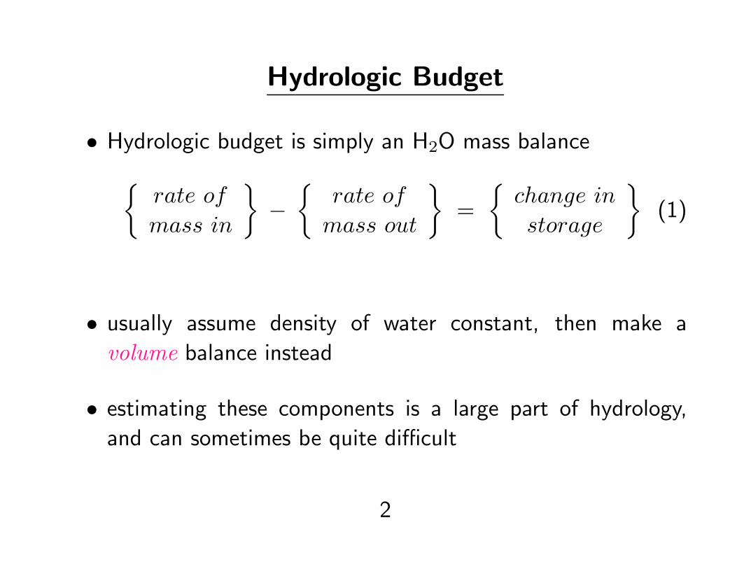
• Hydrologic budget is simply an H2O mass balance{rate of
mass in
}−{
rate of
mass out
}={change in
storage
}(1)
• usually assume density of water constant, then make a
volume balance instead
• estimating these components is a large part of hydrology,
and can sometimes be quite difficult
2
Hydrologic Budget (cont.)
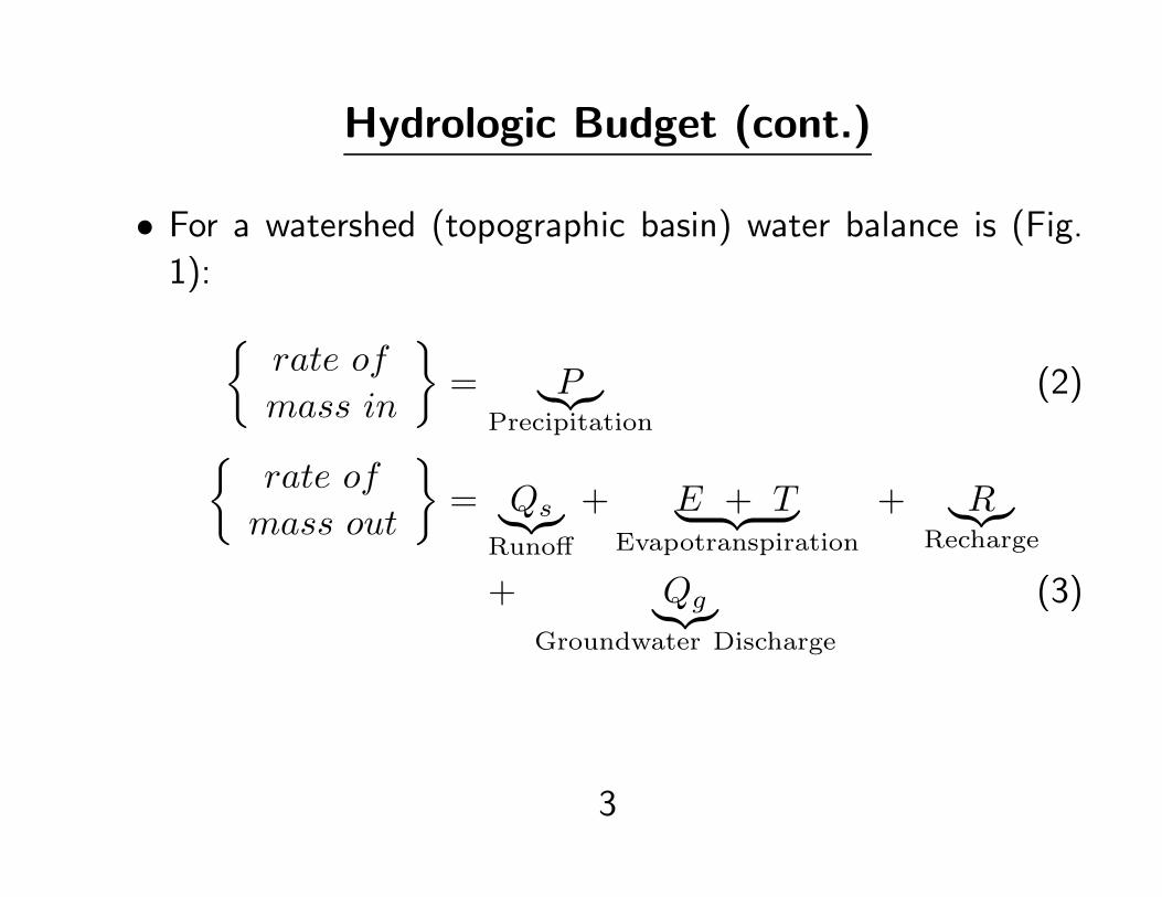
• For a watershed (topographic basin) water balance is (Fig.
1): {rate of
mass in
}= P︸︷︷︸
Precipitation
(2){rate of
mass out
}= Qs︸︷︷︸
Runoff
+ E + T︸ ︷︷ ︸Evapotranspiration
+ R︸︷︷︸Recharge
+ Qg︸︷︷︸Groundwater Discharge
(3)
3
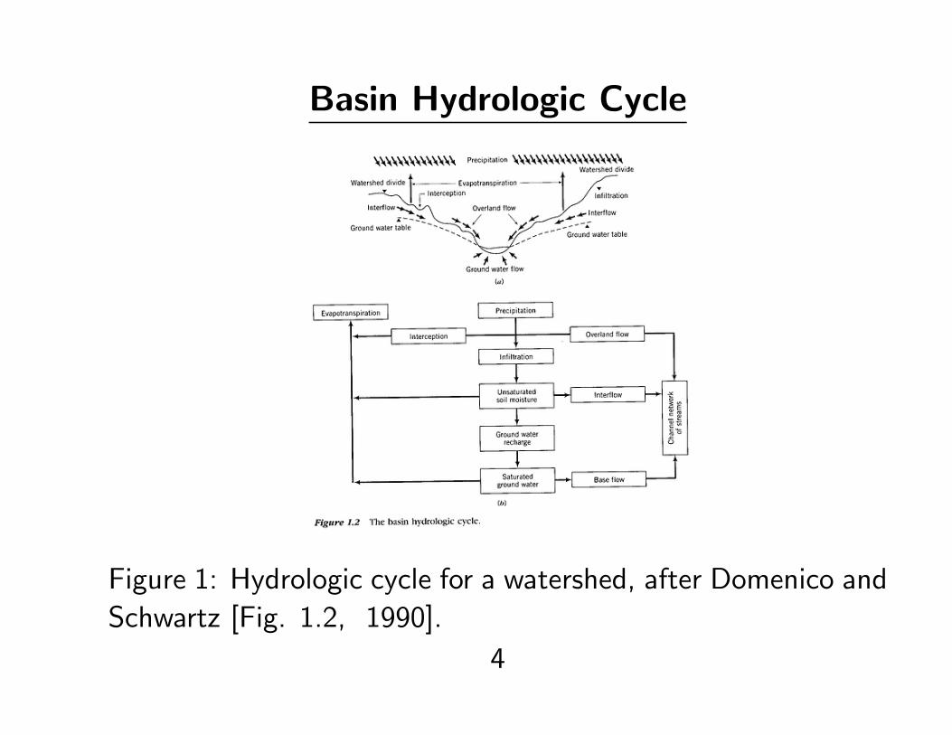
Basin Hydrologic Cycle
Figure 1: Hydrologic cycle for a watershed, after Domenico and
Schwartz [Fig. 1.2, 1990].
4
Evaporation
Misc. information and data sources:
• U.S. Evaporation climatology (calculated)
• U.S. raw evaporation data
• Daily pan (or actual?) evaporation at DFW
lakes
• moisture sensor rebate for NTMWD
customers
5
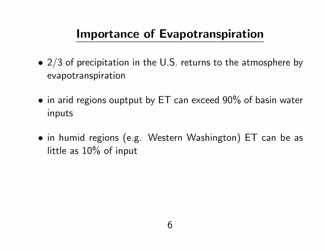
Importance of Evapotranspiration
• 2/3 of precipitation in the U.S. returns to the atmosphere by
evapotranspiration
• in arid regions ouptput by ET can exceed 90% of basin water
inputs
• in humid regions (e.g. Western Washington) ET can be as
little as 10% of input
6
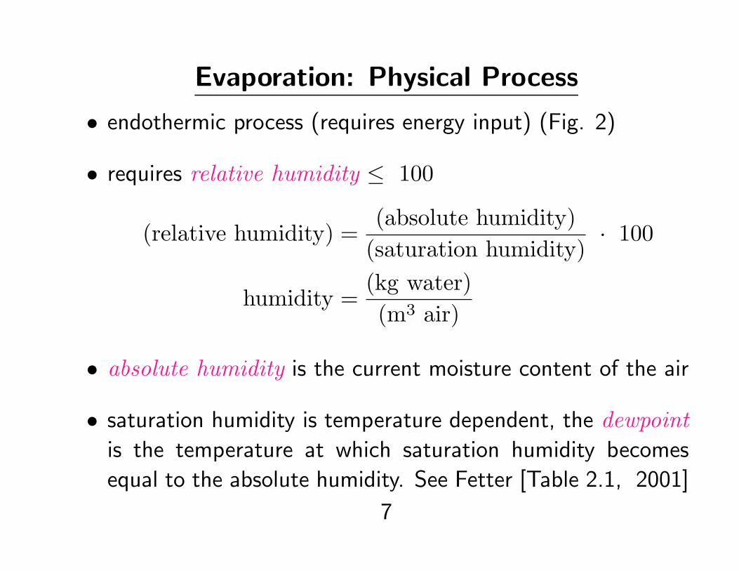
Evaporation: Physical Process
• endothermic process (requires energy input) (Fig. 2)
• requires relative humidity ≤ 100
(relative humidity) =(absolute humidity)
(saturation humidity)· 100
humidity =(kg water)(m3 air)
• absolute humidity is the current moisture content of the air
• saturation humidity is temperature dependent, the dewpointis the temperature at which saturation humidity becomes
equal to the absolute humidity. See Fetter [Table 2.1, 2001]
7
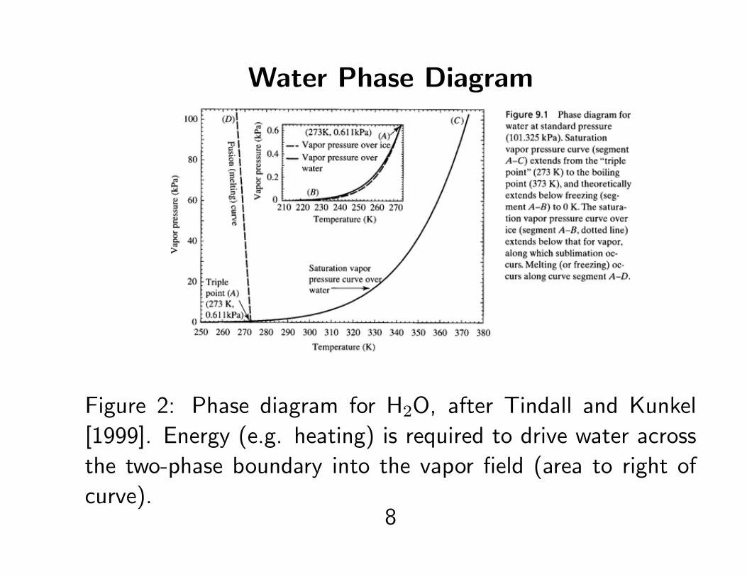
Water Phase Diagram
Figure 2: Phase diagram for H2O, after Tindall and Kunkel
[1999]. Energy (e.g. heating) is required to drive water across
the two-phase boundary into the vapor field (area to right of
curve).8
Evaporation: Measurement
• Direct methods:
– pan evaporation (land pan, Figs. 3–4):
∗ observe evaporation from a standard-sized shallow metal
pan
∗ best to measure precipitation input separately (i.e. make
a quantitative water balance for pan)
∗ apply empirical relationship to estimate lake or plant
evaporation (Fig. 6)
– lysimeter (Fig. 5)
∗ a cannister containing “natural” soil, installed at ground
level
∗ weigh (and perform water balance) to determine moisture
content changes due to evaporation9
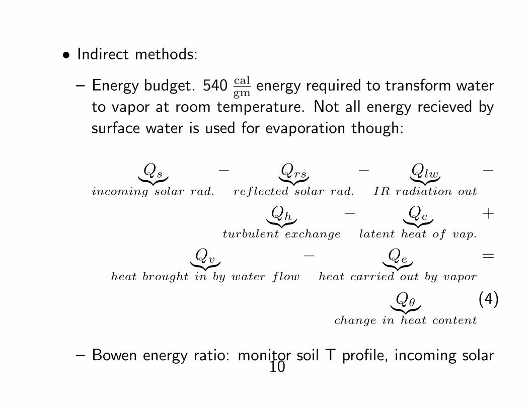
• Indirect methods:
– Energy budget. 540 calgm energy required to transform water
to vapor at room temperature. Not all energy recieved by
surface water is used for evaporation though:
Qs︸︷︷︸incoming solar rad.
− Qrs︸︷︷︸reflected solar rad.
− Qlw︸︷︷︸IR radiation out
−
Qh︸︷︷︸turbulent exchange
− Qe︸︷︷︸latent heat of vap.
+
Qv︸︷︷︸heat brought in by water flow
− Qe︸︷︷︸heat carried out by vapor
=
Qθ︸︷︷︸change in heat content
(4)
– Bowen energy ratio: monitor soil T profile, incoming solar10
radiation and heat radiated to atmosphere at soil surface
(combines Qh & Qe in Eqn. 4, see Hillel [p. 290, 1980]
– Eddy correlation method
∗ directly measure water vapor flux using wind speed,
humidity measurements, i.e. micro-meteorology
∗ more recently used to measure CO2 fluxes, e.g. ABLE
experiment
– soil chloride profile (Cl mass balance, e.g. paleoclimate
studies)
11
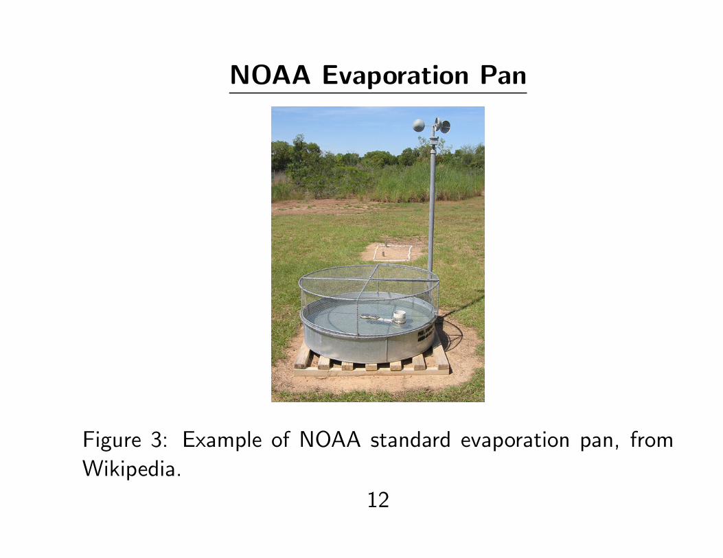
NOAA Evaporation Pan
Figure 3: Example of NOAA standard evaporation pan, from
Wikipedia.
12
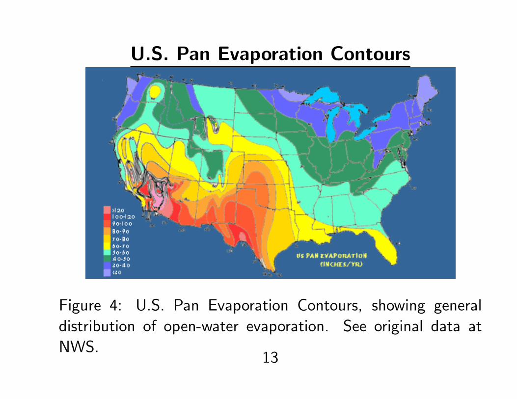
U.S. Pan Evaporation Contours
Figure 4: U.S. Pan Evaporation Contours, showing general
distribution of open-water evaporation. See original data at
NWS.13
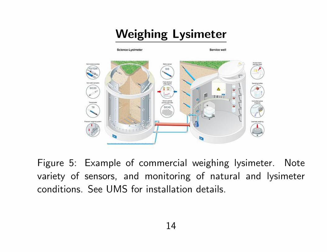
Weighing Lysimeter
Figure 5: Example of commercial weighing lysimeter. Note
variety of sensors, and monitoring of natural and lysimeter
conditions. See UMS for installation details.
14
Transpiration
• Transpiration is evaporation from plants
• underside of leaves contain pores (stoma) which open for
photosynthesis during the day
• water drawn into plant by roots to provide support and
transport nutrients is lost via stoma
• hence length of day is an important constraint on
transpiration
• see animation for a helpful visualization
15
Evapotranspiration: Physical Process
• Transpiration is evaporation from plants
• underside of leaves contain pores (stoma) which open for
photosynthesis during the day
• water drawn into plant by roots to provide support and
transport nutrients is lost via stoma
• hence length of day is an important constraint on
transpiration
• ET is combined bare soil evaporation and plant transpiration16
• transpiration predominant mechanism for water loss from soil
in all but the driest climates [can be 15-80% of basin water
losses, Fetter, 2001] (Fig. 6)
• phreatophytes (plants with roots to water table) are generally
most important, except in agricultural settings
• for shallow-rooted plants, ET ceases when soil moisture drops
below wilting point (plant root suction less than soil suction)
17
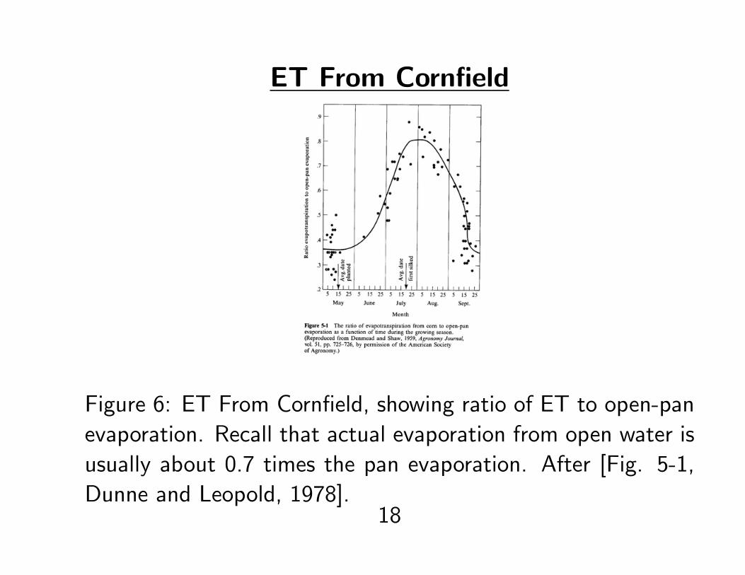
ET From Cornfield
Figure 6: ET From Cornfield, showing ratio of ET to open-pan
evaporation. Recall that actual evaporation from open water is
usually about 0.7 times the pan evaporation. After [Fig. 5-1,
Dunne and Leopold, 1978].18
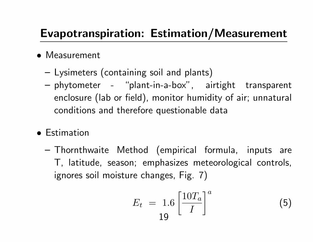
Evapotranspiration: Estimation/Measurement
• Measurement
– Lysimeters (containing soil and plants)
– phytometer - “plant-in-a-box”, airtight transparent
enclosure (lab or field), monitor humidity of air; unnatural
conditions and therefore questionable data
• Estimation
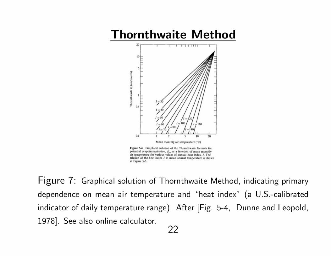
– Thornthwaite Method (empirical formula, inputs are
T, latitude, season; emphasizes meteorological controls,
ignores soil moisture changes, Fig. 7)
Et = 1.6[
10TaI
]a(5)
19
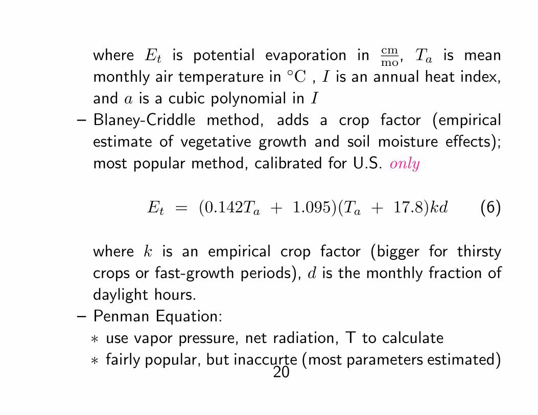
where Et is potential evaporation in cmmo, Ta is mean
monthly air temperature in ◦C , I is an annual heat index,
and a is a cubic polynomial in I
– Blaney-Criddle method, adds a crop factor (empirical
estimate of vegetative growth and soil moisture effects);
most popular method, calibrated for U.S. only
Et = (0.142Ta + 1.095)(Ta + 17.8)kd (6)
where k is an empirical crop factor (bigger for thirsty
crops or fast-growth periods), d is the monthly fraction of
daylight hours.
– Penman Equation:
∗ use vapor pressure, net radiation, T to calculate
∗ fairly popular, but inaccurte (most parameters estimated)20
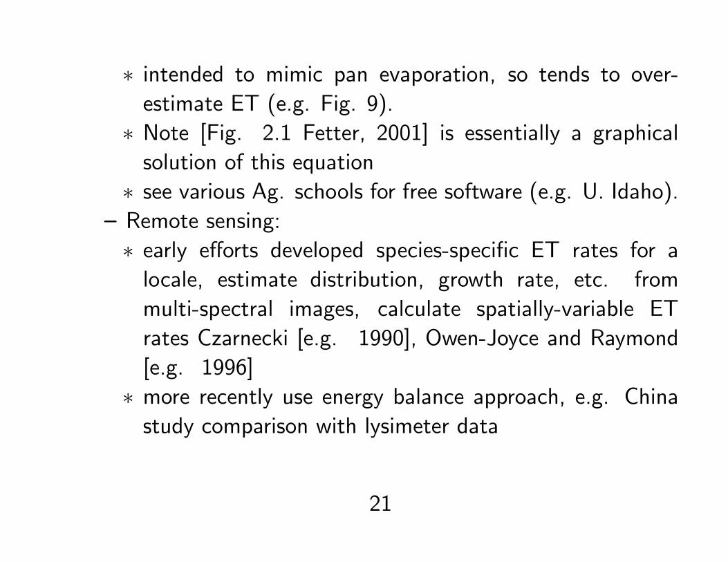
∗ intended to mimic pan evaporation, so tends to over-
estimate ET (e.g. Fig. 9).
∗ Note [Fig. 2.1 Fetter, 2001] is essentially a graphical
solution of this equation
∗ see various Ag. schools for free software (e.g. U. Idaho).
– Remote sensing:
∗ early efforts developed species-specific ET rates for a
locale, estimate distribution, growth rate, etc. from
multi-spectral images, calculate spatially-variable ET
rates Czarnecki [e.g. 1990], Owen-Joyce and Raymond
[e.g. 1996]
∗ more recently use energy balance approach, e.g. China
study comparison with lysimeter data
21
Thornthwaite Method
Figure 7: Graphical solution of Thornthwaite Method, indicating primary
dependence on mean air temperature and “heat index” (a U.S.-calibrated
indicator of daily temperature range). After [Fig. 5-4, Dunne and Leopold,
1978]. See also online calculator.22
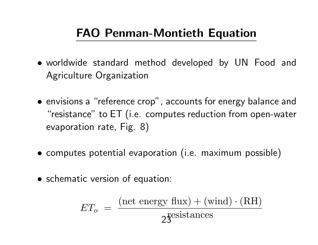
FAO Penman-Montieth Equation
• worldwide standard method developed by UN Food and
Agriculture Organization
• envisions a “reference crop”, accounts for energy balance and
“resistance” to ET (i.e. computes reduction from open-water
evaporation rate, Fig. 8)
• computes potential evaporation (i.e. maximum possible)
• schematic version of equation:
ETo =(net energy flux) + (wind) · (RH)
resistances23
where the energy flux is solar input minus infrared radiation
and reflection out, resistances are rs and ra as shown in Fig.
8
24
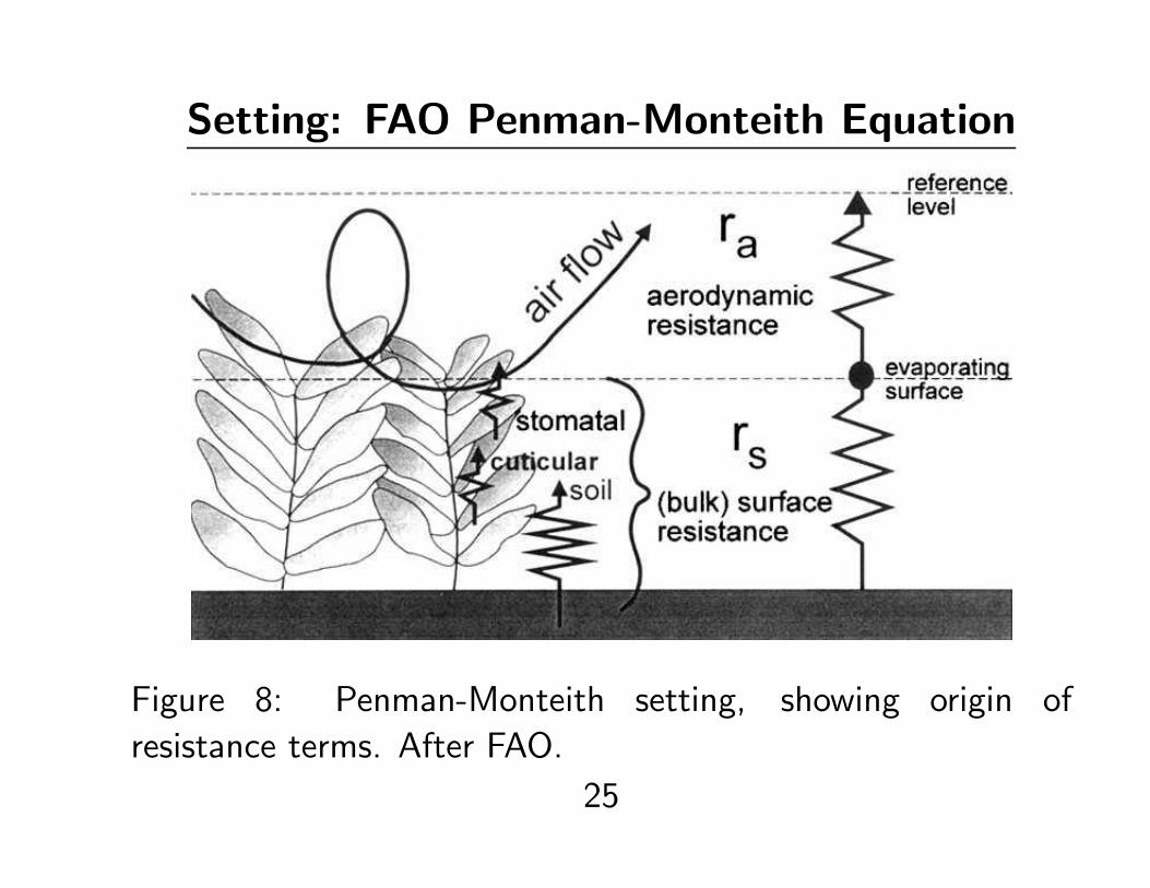
Setting: FAO Penman-Monteith Equation
Figure 8: Penman-Monteith setting, showing origin of
resistance terms. After FAO.
25
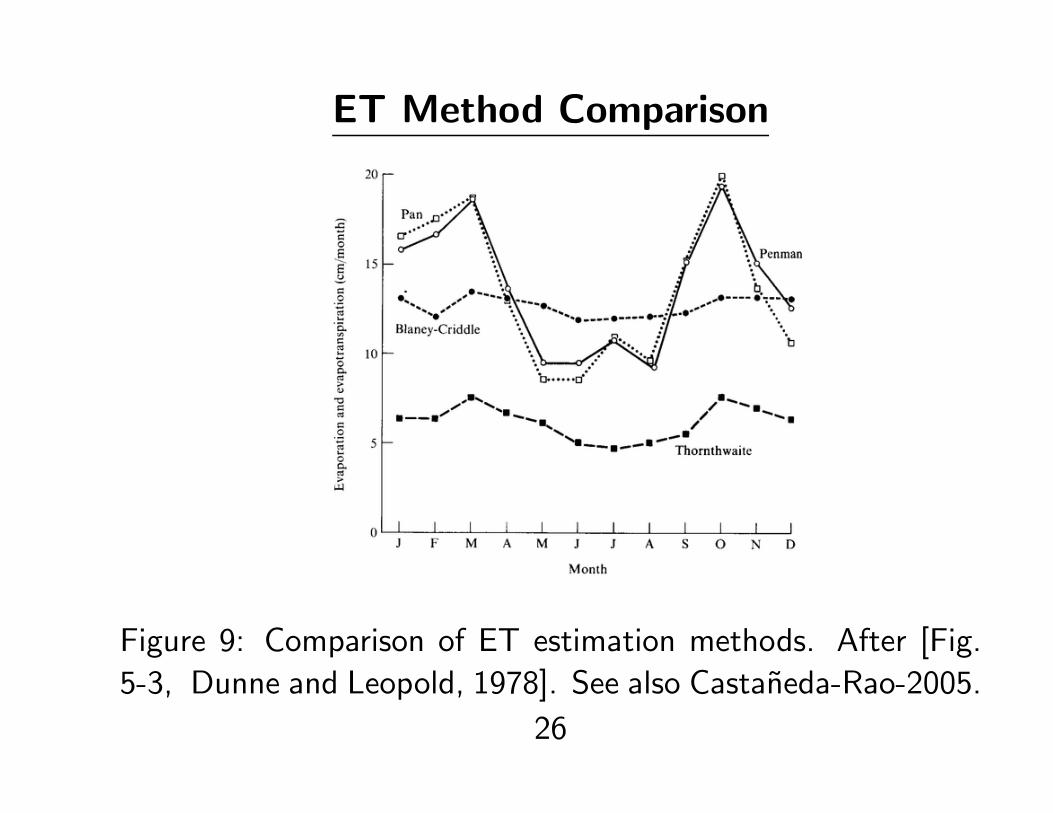
ET Method Comparison
Figure 9: Comparison of ET estimation methods. After [Fig.
5-3, Dunne and Leopold, 1978]. See also Castaneda-Rao-2005.
26
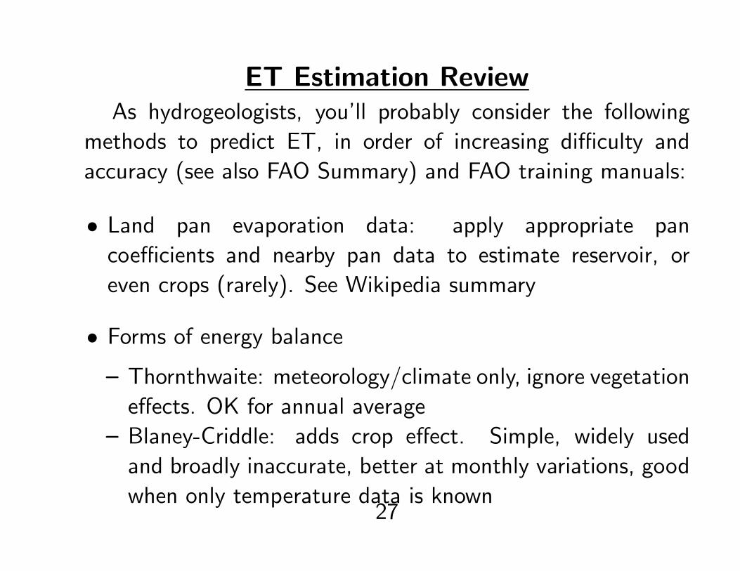
ET Estimation ReviewAs hydrogeologists, you’ll probably consider the following
methods to predict ET, in order of increasing difficulty and
accuracy (see also FAO Summary) and FAO training manuals:
• Land pan evaporation data: apply appropriate pan
coefficients and nearby pan data to estimate reservoir, or
even crops (rarely). See Wikipedia summary
• Forms of energy balance
– Thornthwaite: meteorology/climate only, ignore vegetation
effects. OK for annual average
– Blaney-Criddle: adds crop effect. Simple, widely used
and broadly inaccurate, better at monthly variations, good
when only temperature data is known27
– Penman: original Penman eqn. mimics pan evaporation
curve, accounts for radiation and convective (wind) flux,
i.e. most terms in (4)
– Penman-Monteith: world standard, assumes realistic
“reference crop”. Provides most inter-comparable results.
28
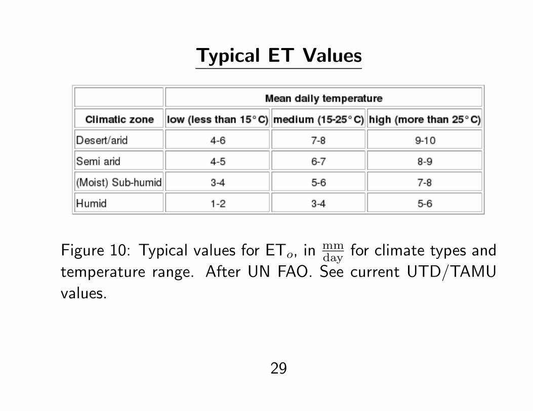
Typical ET Values
Figure 10: Typical values for ETo, in mmday for climate types and
temperature range. After UN FAO. See current UTD/TAMU
values.
29
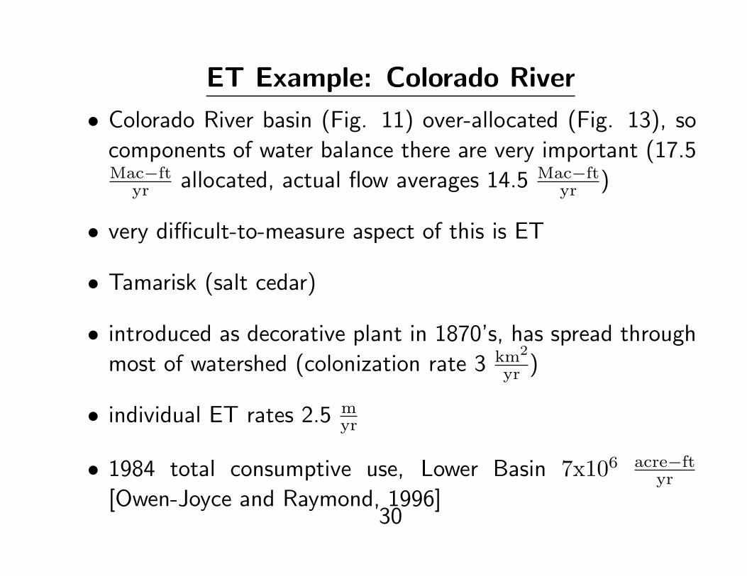
ET Example: Colorado River
• Colorado River basin (Fig. 11) over-allocated (Fig. 13), so
components of water balance there are very important (17.5Mac−ft
yr allocated, actual flow averages 14.5 Mac−ftyr )
• very difficult-to-measure aspect of this is ET
• Tamarisk (salt cedar)
• introduced as decorative plant in 1870’s, has spread through
most of watershed (colonization rate 3 km2
yr )
• individual ET rates 2.5 myr
• 1984 total consumptive use, Lower Basin 7x10⁶ acre−ftyr
[Owen-Joyce and Raymond, 1996]30
• of that 15% lost through ET, 6% by natural phreatophytes
(primarily tamarisk), 18% exported to AZ, 67% exported to
CA
• see USGS biennial consumptive use studies
31
Tamarisk Invasion/Control
• current distribution monitored by USGS
• other organizations organize remediation (e.g. Tamarisk
Coalition)
• see TRO Assessment report 2008 for current status of
mitigation/impact
32
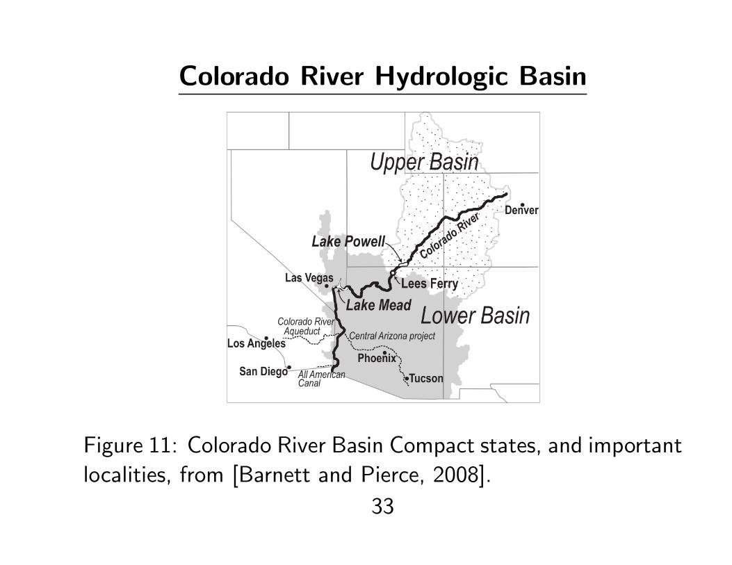
Colorado River Hydrologic Basin
Figure 11: Colorado River Basin Compact states, and important
localities, from [Barnett and Pierce, 2008].
33
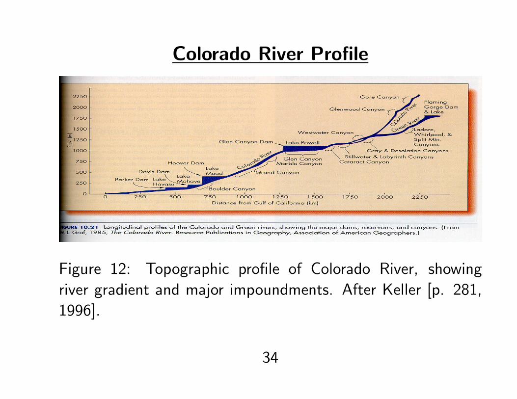
Colorado River Profile
Figure 12: Topographic profile of Colorado River, showing
river gradient and major impoundments. After Keller [p. 281,
1996].
34
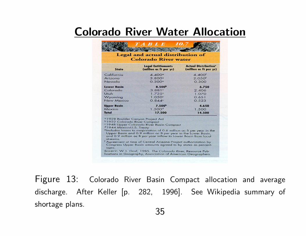
Colorado River Water Allocation
Figure 13: Colorado River Basin Compact allocation and average
discharge. After Keller [p. 282, 1996]. See Wikipedia summary of
shortage plans.35
Evaporation and Climate Change
36
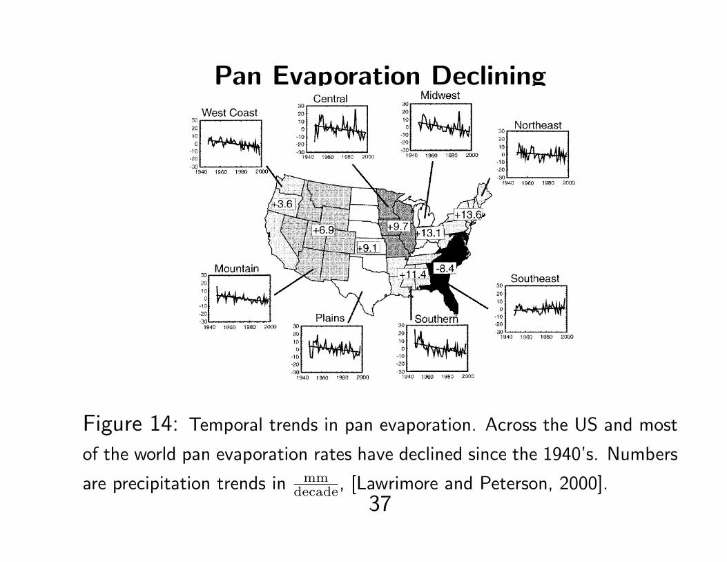
Pan Evaporation Declining
Figure 14: Temporal trends in pan evaporation. Across the US and most
of the world pan evaporation rates have declined since the 1940’s. Numbers
are precipitation trends in mmdecade, [Lawrimore and Peterson, 2000].
37
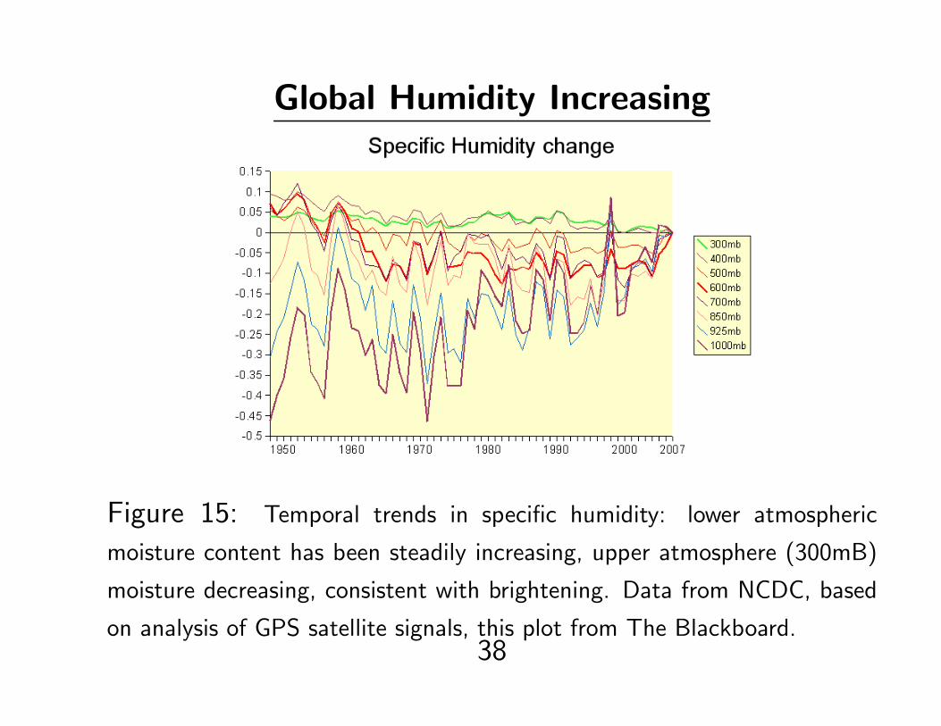
Global Humidity Increasing
Figure 15: Temporal trends in specific humidity: lower atmospheric
moisture content has been steadily increasing, upper atmosphere (300mB)
moisture decreasing, consistent with brightening. Data from NCDC, based
on analysis of GPS satellite signals, this plot from The Blackboard.38
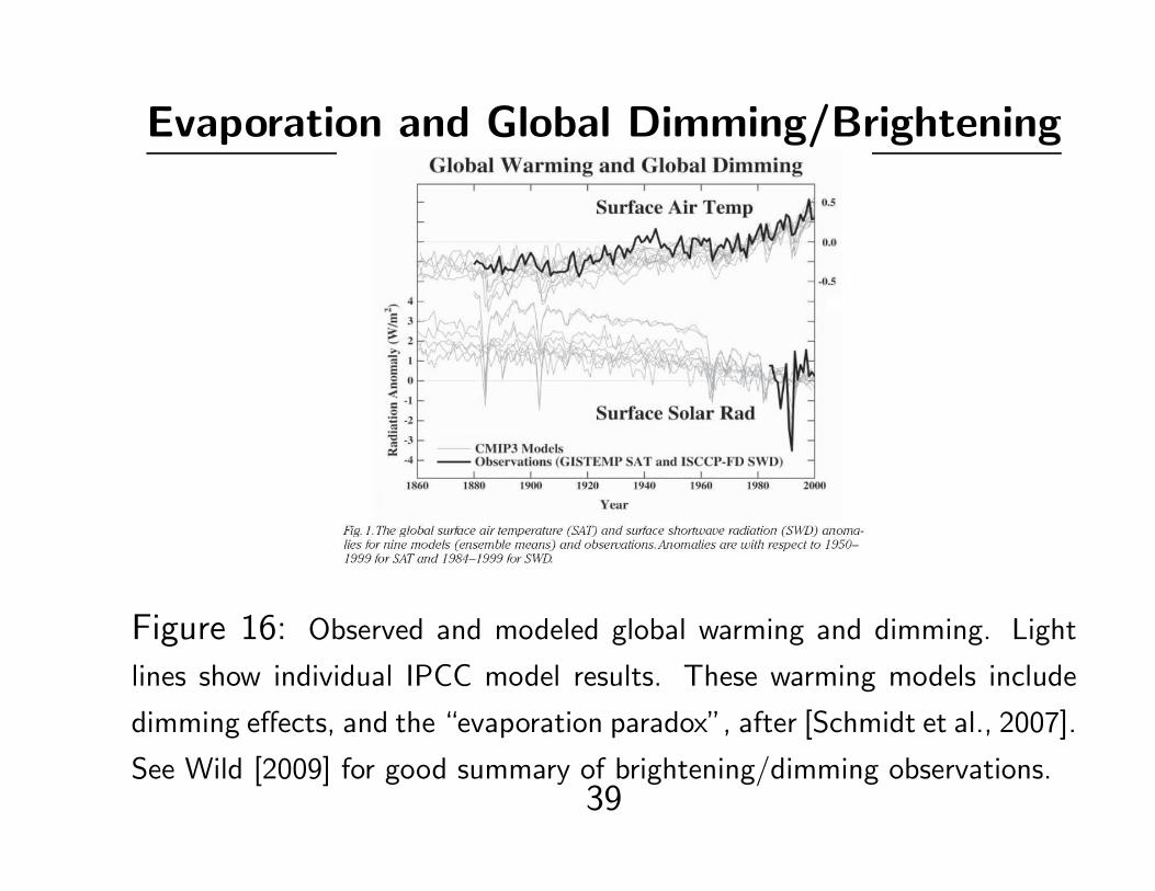
Evaporation and Global Dimming/Brightening
Figure 16: Observed and modeled global warming and dimming. Light
lines show individual IPCC model results. These warming models include
dimming effects, and the “evaporation paradox”, after [Schmidt et al., 2007].
See Wild [2009] for good summary of brightening/dimming observations.39
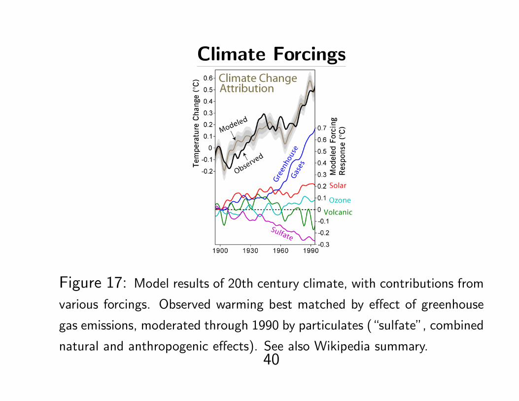
Climate Forcings
Figure 17: Model results of 20th century climate, with contributions from
various forcings. Observed warming best matched by effect of greenhouse
gas emissions, moderated through 1990 by particulates (“sulfate”, combined
natural and anthropogenic effects). See also Wikipedia summary.40
Precipitation
Useful data sources:
• National Weather Service flood prediction
data
• Intellicast TX-OK 7-day cumulative precip
from NEXRAD data
• Intellicast current hourly lightning strikes
41
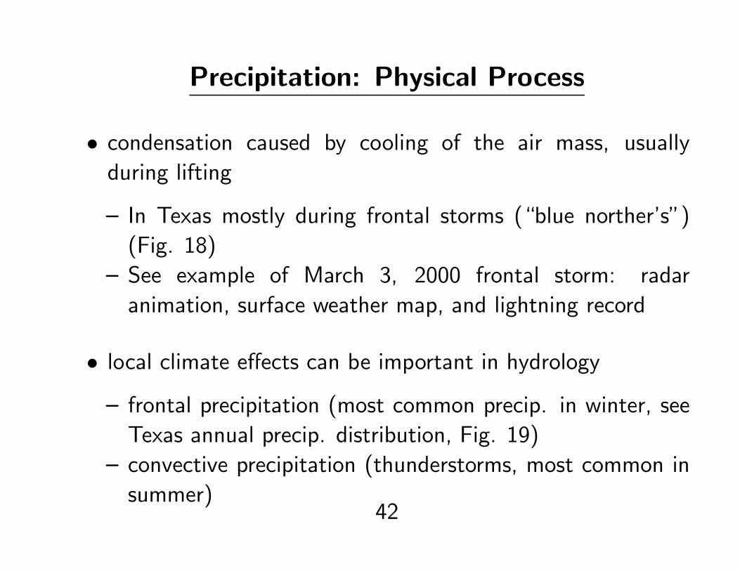
Precipitation: Physical Process
• condensation caused by cooling of the air mass, usually
during lifting
– In Texas mostly during frontal storms (“blue norther’s”)
(Fig. 18)
– See example of March 3, 2000 frontal storm: radar
animation, surface weather map, and lightning record
• local climate effects can be important in hydrology
– frontal precipitation (most common precip. in winter, see
Texas annual precip. distribution, Fig. 19)
– convective precipitation (thunderstorms, most common in
summer)42
– e.g. in temperate arid regions snow is predominant
recharge contributer, even if not predominant form of
precip.
– orographic effect: heavier precip. on upwind side of
topographic highs, lower than average on downwind side
– coastal states often affected by tropical cyclones (e.g.
similar effect from upper atmosphere low at DFW 2009,
Fig. 20)
43
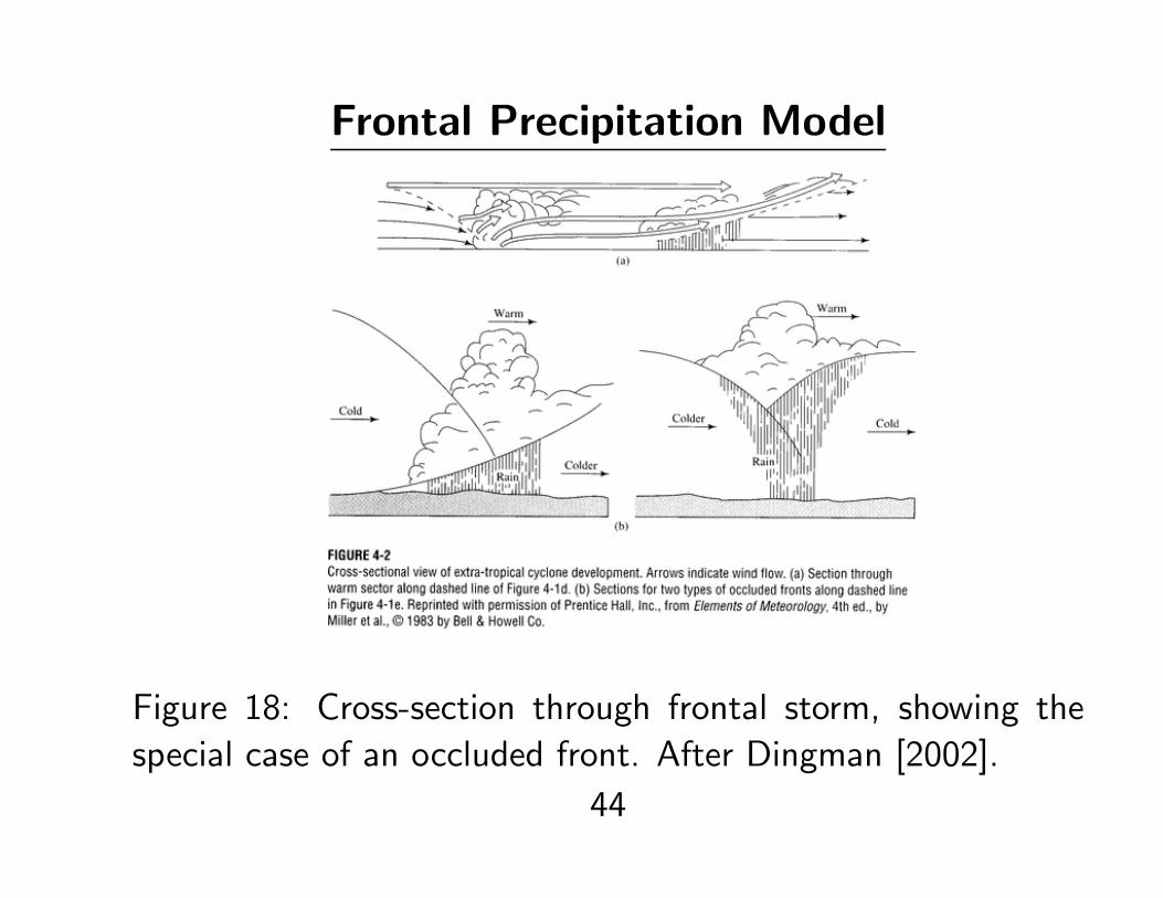
Frontal Precipitation Model
Figure 18: Cross-section through frontal storm, showing the
special case of an occluded front. After Dingman [2002].
44
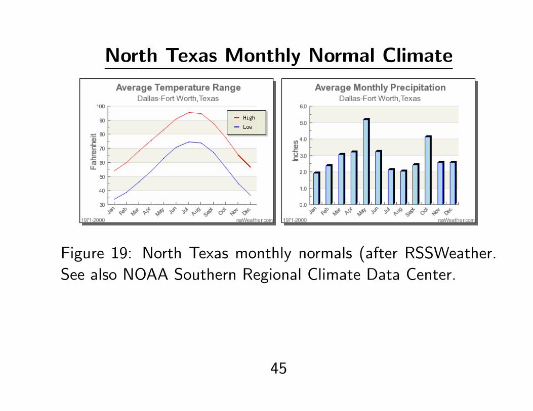
North Texas Monthly Normal Climate
Figure 19: North Texas monthly normals (after RSSWeather.
See also NOAA Southern Regional Climate Data Center.
45
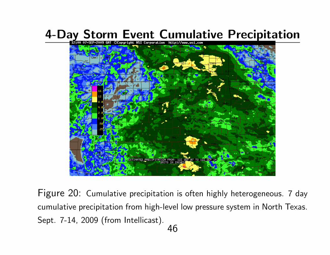
4-Day Storm Event Cumulative Precipitation
Figure 20: Cumulative precipitation is often highly heterogeneous. 7 day
cumulative precipitation from high-level low pressure system in North Texas.
Sept. 7-14, 2009 (from Intellicast).46
Precipitation: Measurement
One of the most easily measured hydrologic cycle fluxes
• NOAA uses a variety of automated gauges (Fig. 21)
• see modern summary at Wikipedia and summary of
automated airport weather stations, the “gold standard”
of weather data worldwide
• Two basic station networks: primary monitoring stations
(usually major airports) and cooperative stations (usually
not run by NOAA, data quality uncertain). See Fig. 22
• this data accessible for free from .edu IP addresses at National
Climate Data Center (NCDC)
47
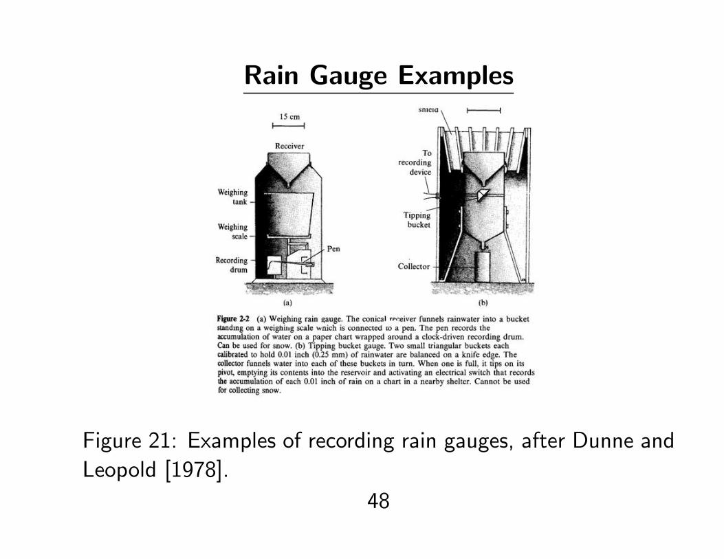
Rain Gauge Examples
Figure 21: Examples of recording rain gauges, after Dunne and
Leopold [1978].
48
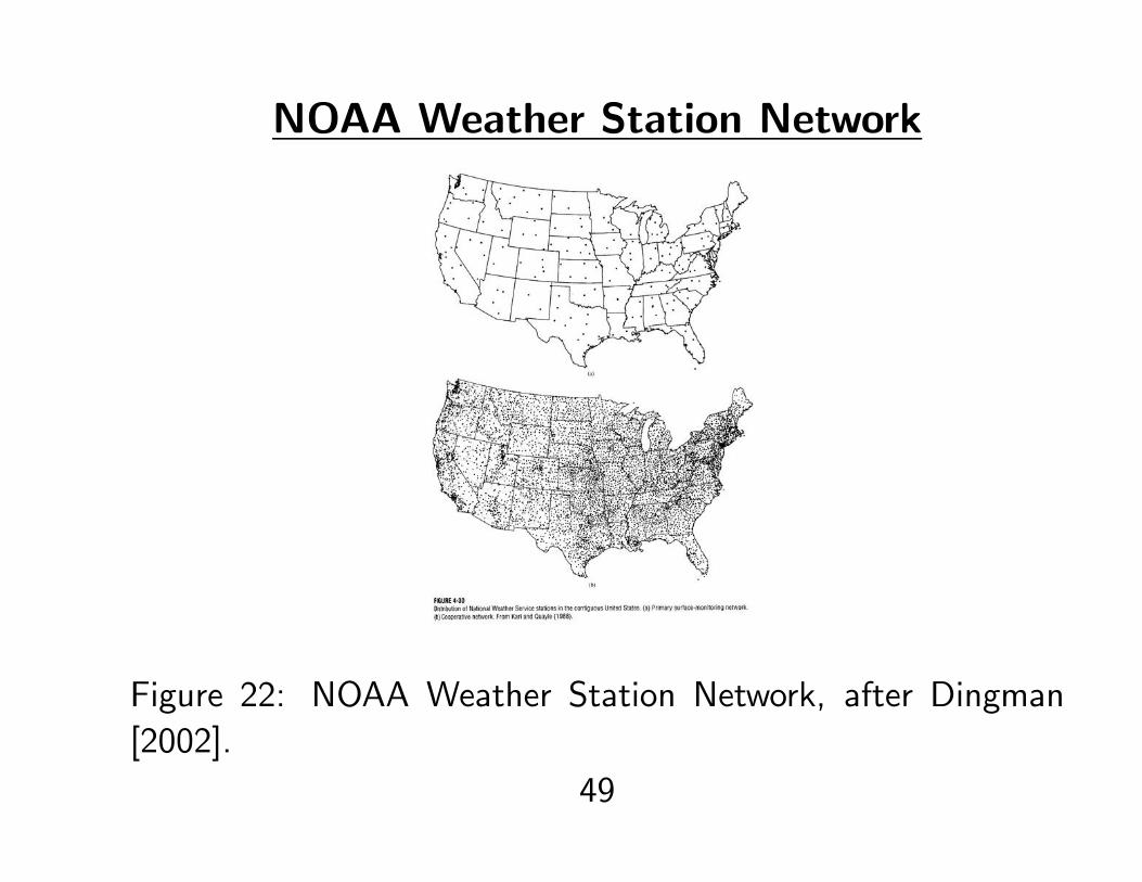
NOAA Weather Station Network
Figure 22: NOAA Weather Station Network, after Dingman
[2002].
49
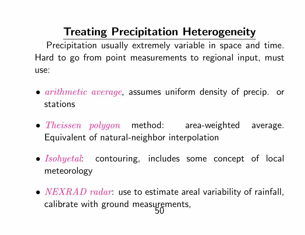
Treating Precipitation HeterogeneityPrecipitation usually extremely variable in space and time.
Hard to go from point measurements to regional input, must
use:
• arithmetic average, assumes uniform density of precip. or
stations
• Theissen polygon method: area-weighted average.
Equivalent of natural-neighbor interpolation
• Isohyetal: contouring, includes some concept of local
meteorology
• NEXRAD radar: use to estimate areal variability of rainfall,
calibrate with ground measurements,50
– accuracy can be controversial, but now standard for runoff
models (see Applied Surface Water Modeling Notes re:
NEXRAD)
– cumulative estimates avaliable nationwide (intended for
flood prediction) at NCDC Hydro Prediction Service
51
Engineering Characterization of Precipitation
See Applied Surface Water Modeling Notes topics:
• Introduction: Design approaches in treating rainfall
• Rainfall data adjustments
• Rainfall data sources (online data)
52

Recharge
53
Recharge
• Physical processes
– infiltration - losses = recharge
– infiltration = precipitation - runoff
– runoff occurs when precip. exceeds infiltration capacity of
soil (Hortonian overland flow)
• Measurement
– Direct: lysimeters
– Indirect
∗ Water table fluctuation
· assumes changes in water level in shallow wells reflect
recharge54
· see USGS summary
· also computer program to develop Master Recession
Curve for well water levels
∗ Chemical mass balance: Cl, 3H, δD , δ18O
· Cl method (assumes all input is atmospheric, OK if
no Cl-sediments in basin; N.B. Cl = 0 in evaporated
water) [Dettinger, 1989]
CII︸︷︷︸Infiltrated mass
+ CPP︸ ︷︷ ︸Precipitation
+ CQQ︸ ︷︷ ︸Runoff
= 0
I =PCPCI
− QCQCI
(7)
· Also note that in many desert basins the runoff is 0,
simplifying (7)
∗ Determine Baseflow (hydrograph separation)55
∗ Use empirical relations based on other basins: e.g.
Maxey-Eakin [Watson et al., 1976], uses rainfall and
elevation maps to estimate recharge, calibrated to basins
of “known” recharge
• see excellent summary of methods and results for desert
basins [Hogan et al., 2004] (and online review)
56

Bibliography
57
Tim P. Barnett and David W. Pierce. When will Lake Mead go dry? Water Resour. Res., 44(W03201), 29 March 2008. doi: 10.1029/2007WR006704. URL http://www.agu.org/journals/pip/wr/2007WR006704-pip.pdf.
J. B. Czarnecki. Geohydrology and evapotranspiration at franklin lake playa, inyo county,california. Ofr 90-356, Denver, CO, 1990.
M. D. Dettinger. Reconnaissance estimates of natural recharge to desert basins in nevada, u.s.a., by using chloride-balance calculations. J. Hydrol., 106:55–78, 1989.
S. L. Dingman. Physical Hydrology. Prentice Hall, Upper Saddle River, NJ, 07458, 2nd edition,2002. ISBN 0-13-099695-5.
P. A. Domenico and F. W. Schwartz. Physical and Chemical Hydrogeology. John Wiley &Sons, New York, 1990. ISBN 0-471-50744-X.
T. Dunne and L. B. Leopold. Water in Environmental Planning. W. H. Freeman, New York,1978. ISBN 0-7167-0079-4.
C. W. Fetter. Applied Hydrogeology. Prentice Hall, Upper Saddle River, NJ, 4th edition, 2001.ISBN 0-13-088239-9.
D. Hillel. Applications of soil physics. Academic Press, New York, 1980. ISBN 0-12-348580-0.
James F. Hogan, Fred M. Phillips, and Bridget R. Scanlon, editors. Groundwater Rechargein a Desert Environment: The Southwestern United States, volume 9 of Water Scienceand Application. Amer. Geophys. Union, 2004. URL http://www.agu.org/cgi-bin/agubooks?topic=AL&book=HYWS0093584&search=Scanlon.
E. A. Keller. Environmental Geology. Prentice Hall, Upper Saddle River, NJ, 1996. 7th Ed.,ISBN 0-02-363281-X.
Jay H. Lawrimore and Thomas C. Peterson. Pan evaporation trends in dry andhumid regions of the united states. Journal of Hydrometeorology, 1(6):543, 2000.ISSN 1525755X. URL http://search.ebscohost.com/login.aspx?direct=true&db=a9h&AN=5716377&site=ehost-live.
58
S. J. Owen-Joyce and L. H. Raymond. An accounting system for water and consumptive usealong the colorado river, hoover dam to mexico. Water-supply paper, U.S. Geol. Survey,Washington, D.C., 1996.
G. A. Schmidt, A. Romanou, and B. Liepert. Further comment on ”a perspective on globalwarming, dimming, and brightening”. EOS, 88(45):473, 11 2007.
J. A. Tindall and J. R. Kunkel. Unsaturated Zone Hydrology for Scientists and Engineers.Prentice-Hall, Upper Saddle River, N.J., 1999. ISBN 0-13-660713-6.
P. Watson, P. Sinclair, and R. Waggoner. Quantitative evaluation of a method for estimatingrecharge to the desert basins of nevada. J. Hydrol., 31:335–357, 1976.
M. Wild. Global dimming and brightening: A review. J. Geophys. Res., 114, 2009. doi:10.1029/2008JD011470.
59
Recommended