Hybrid simulation modeling for regional food systems
by
Anuj Mittal
A thesis submitted to the graduate faculty
in partial fulfillment of the requirements for the degree of
MASTER OF SCIENCE
Major: Industrial Engineering
Program of Study Committee:
Caroline C. Krejci, Major Professor
Michael C. Dorneich
Richard T. Stone
David E. Cantor
Iowa State University
Ames, Iowa
2016
Copyright © Anuj Mittal, 2016. All rights reserved.

ii
DEDICATION
I would like to dedicate this thesis to my parents for their continuous support and
motivation.

iii
TABLE OF CONTENTS
Page
LIST OF FIGURES ................................................................................................... v
LIST OF TABLES ..................................................................................................... ix
NOMENCLATURE .................................................................................................. x
ACKNOWLEDGMENTS ......................................................................................... xi
ABSTRACT………………………………. .............................................................. xii
CHAPTER 1 INTRODUCTION .......................................................................... 1
Regional Food ...................................................................................................... 1
Evaluating Supply Chain Performance ................................................................ 7
Motivation for This Study .................................................................................... 9
Thesis Organization ............................................................................................. 11
References………… ............................................................................................ 13
CHAPTER 2 LITERATURE REVIEW ............................................................... 17
Supply Chain Management .................................................................................. 17
Simulation in Supply Chain Management ........................................................... 18
ABM vs DES – A Long Controversy .................................................................. 24
Hybrid Simulation ................................................................................................ 28
Empirical Simulation Models .............................................................................. 29
Evaluating RFSC Performance ............................................................................ 30
References………… ............................................................................................ 32
CHAPTER 3 HYBRID SIMULATION MODEL ................................................ 37
Agent-Based Model ............................................................................................. 39
Discrete Event Simulation ................................................................................... 56
Hybrid Simulation Model .................................................................................... 64
References ......................................................................................................... 80
CHAPTER 4 SIMULATION RESULTS AND DISCUSSION ........................... 83
Verification of the hybrid simulation model ........................................................ 83
Model I – Status Quo ........................................................................................... 84

iv
Food Hub Interventions ....................................................................................... 94
References ......................................................................................................... 106
CHAPTER 5 CONCLUSIONS AND FUTURE WORK ..................................... 107
General Conclusions ............................................................................................ 107
Limitations and Future Work ............................................................................... 109
APPENDIX A - PRODUCER SURVEY .................................................................. 111
APPENDIX B - AGGLOMERATIVE SCHEDULE ................................................ 117

v
LIST OF FIGURES
Page
Figure 1 Flowchart of research motivation .............................................................. 12
Figure 2 A typical supply chain structure ................................................................ 18
Figure 3 Process-oriented approach of DES ............................................................ 19
Figure 4 Heterogeneous agents interacting with each other and with the
environment in a typical ABM .................................................................. 21
Figure 5 A system dynamics model of “product diffusion” in the form of a stock
and flow diagram ...................................................................................... 23
Figure 6 Timeline diagram describing four stages in an order cycle at the food hub 38
Figure 7 Hybrid simulation (ABM-DES) model overview ...................................... 39
Figure 8 Dendrogram for hierarchical cluster analysis from producers’ survey data 45
Figure 9 Survey data showing the effect of other deliveries and activities in the
area near to the food hub on producers’ decision to schedule the delivery 49
Figure 10 Survey data showing the effect of harvesting schedule on producers’
decision to schedule the delivery ............................................................... 50
Figure 11 Satisfaction level of 24 survey respondents to deliver the products in
11 time slots ............................................................................................... 51
Figure 12 Survey data showing satisfaction level of 24 producers for the 7 different
waiting times range at the food hub ........................................................... 53
Figure 13 Variation of UC vs waiting time for each cluster ....................................... 54
Figure 14 Receiving process at the food hub ............................................................. 56
Figure 15 Storage of “NON” goods at the food hub .................................................. 58
Figure 16 Storage of “FROZ” goods at the food hub................................................. 59
Figure 17 Storage of “REF” goods at the food hub ................................................... 59
Figure 18 Facility layout of the food hub ................................................................... 60

vi
Figure 19 Flowchart of the Arena simulation model ................................................. 63
Figure 20 ABM- DES model overview (Status Quo) ................................................ 67
Figure 21 Priority delivery option to the producers who schedule their delivery
times in advance ......................................................................................... 69
Figure 22 Survey data showing the effect of priority queue option on the scheduling
decision of the producers ........................................................................... 70
Figure 23 Producer decision-making process with priority delivery option .............. 71
Figure 24 Snapshot of the Arena simulation model flowchart with priority delivery
option ......................................................................................................... 72
Figure 25 Hybrid simulation (ABM-DES-ABM) model overview with priority
delivery option ........................................................................................... 73
Figure 26 Hybrid simulation (ABM-DES-ABM) model overview with food hub
agent ........................................................................................................... 74
Figure 27 Hybrid simulation (ABM-DES-ABM) model overview with monetary
incentives and priority delivery option ...................................................... 75
Figure 28 Survey data showing the effect of monetary incentives on producers
scheduling decision .................................................................................... 76
Figure 29 Survey data showing satisfaction level of the survey respondents with
respect to doing business with the food hub .............................................. 77
Figure 30 Survey data showing how often producers share their business experience
with food hub with the other food hub producers ...................................... 79
Figure 31 NetLogo model showing food hub – producer and producer-producer
interactions ................................................................................................. 80
Figure 32 Number of producers scheduling the delivery in each time step for
Scenario 1, 2 and 3 of Model I ................................................................... 86
Figure 33 Number of producers arriving in each time slot for Scenario 1 of Model I 88
Figure 34 Comparison of number of producers arriving and scheduling the delivery
on day 1 and day 2 for Scenario 1 of Model I .......................................... 89
Figure 35 Average number of producers not scheduling their deliveries due to
multiple deliveries and harvesting schedule for Scenario 1 of Model 1 .... 90
vii
Figure 36 Average man hour utilization rate on day 1 and day 2 for Scenario 1
of Model I ................................................................................................. 91
Figure 37 Average queue time on day 1 and day 2 for Scenario 1 of Model I .......... 91
Figure 38 Average queue time vs number of producers scheduling the delivery
on day 1 for Scenarios 1, 2, and 3 of Model I ............................................ 93
Figure 39 Average queue time vs number of producers scheduling the delivery
on day 2 for Scenarios 1, 2, and 3 of Model I ............................................ 93
Figure 40 Number of producers scheduling and benefiting from the priority
delivery incentive in each time step of Model II ....................................... 95
Figure 41 Average overall number of producers scheduling and benefiting from
the priority delivery incentive in Model II ................................................. 95
Figure 42 Number of producers scheduling in each time step in Model II due to
benefits of priority delivery in the previous cycle ..................................... 96
Figure 43 Average number of producers scheduling and benefiting from the priority
delivery incentive if the food hub puts capacity limit on the time
slots in Model II ......................................................................................... 97
Figure 44 Number of producers arriving in each time slot when the food hub
provides priority delivery benefit to the producers for scheduling
(Model II) versus the status quo (Model I) ................................................. 98
Figure 45 Number of producers scheduling the delivery and percentage monetary
incentive of a producer total sales provided by the food hub in each
time step of Model III ................................................................................ 100
Figure 46 Average queue time on day 1 and day 2 if the food hub provides
monetary incentive benefits to the scheduling producers in Model III ..... 100
Figure 47 Number of producers arriving in each time slot when the food hub
provides monetary incentives to the producers for scheduling
(Model III) versus the status quo (Model I) ............................................... 102
Figure 48 Comparison of number of producers who are not affected by monetary
incentives provided by the food hub but schedule due to benefits of
priority delivery in the previous cycle in Model III vs number of
producers who schedule the delivery due to priority delivery option
in Model II (without capacity limit on time slots) .................................... 103

viii
Figure 49 Number of producers scheduling the delivery in each time step when
the food hub provides feedback to the producers and producers interact
with each other to share information in Model IV ..................................... 104
Figure 50 Number of successful food hub-producer and producer-producer
interactions in Model IV ............................................................................ 105
Figure 51 Number of successful interactions between the food hub and a producer
and between two producers in Model IV ................................................... 105
Figure 52 Number of producers arriving in each time slot when food hub provide
provides feedback to the producers for scheduling (Model IV) versus
the status quo (Model I) ............................................................................. 106

ix
LIST OF TABLES
Page
Table 1 Comparison of three most popular simulation techniques in supply chain
management ............................................................................................... 26
Table 2 Behavioral response of four clusters to six attributes ................................ 47
Table 3 ABM variables ........................................................................................... 54
Table 4 ABM parameters ........................................................................................ 55
Table 5 Four different types of product categories at the food hub ........................ 57
Table 6 Description of data for each of the four product categories....................... 61
Table 7 Receiving time values for all the three product categories ........................ 62
Table 8 DES variables............................................................................................. 63
Table 9 DES parameters ......................................................................................... 64
Table 10 Summary of number of producers scheduling the delivery for Model I.... 86
Table 11 Statistical analysis of the outcomes of three tested scenarios in Model I .. 87

x
NOMENCLATURE
DES Discrete Event Simulation
ABM Agent-Based Model
SD System Dynamics
RFSC Regional Food Supply Chains

xi
ACKNOWLEDGMENTS
First and foremost, I would like to thank my major professor Dr. Caroline C. Krejci
for her continuous encouragement and confidence in me. She has been a great help in making
me learn on how to prioritize work in life. I would sincerely like to express my respect and
gratitude to her for inspiring me from time to time and making my first research experience
really enjoyable.
I would also like to thank my committee members, Dr. Michael C. Dorneich, Dr.
Richard T. Stone and Dr. David E. Cantor for their guidance and support throughout the
course of this research. I want to specially thank them for providing their valuable inputs and
guidance in designing and conducting the survey for this research study.
I would also like to thank my great friend Akshit Peer for his help and suggestions
while writing this thesis. A special thanks to Gary Huber for his contribution towards his
thesis and making my research smooth. I would also like to thank Leopold Center for
Sustainable Agriculture for partially funding this research.
In addition, I would also like to thank my friends at Iowa State, colleagues, Hardik
Bora and Teri Craven, the department faculty and staff for making my time at Iowa State
University a wonderful experience. I want to also offer my appreciation to those who were
willing to participate in my surveys and observations, without whom, this thesis would not
have been possible.
Finally, a big thank you to Dr. Saurabh, Dr. Surabhi, Sarthak, Samarth, Alisha and
Ankur for their encouragement, patience and love.

xii
ABSTRACT
In response to concerns regarding the serious environmental and social issues
associated with conventional food distribution systems, consumer demand for regionally-
produced food is growing. Regional food hubs are playing a critical role in meeting this
growing demand. Food hubs aggregate, distribute, and market regionally-produced food,
with a goal of promoting and supporting environmental and social sustainability. They
provide an alternative distribution channel through which small and mid-sized producers can
access wholesale markets, and they improve consumer access to regional food at competitive
prices. Despite the benefits they provide, food hubs struggle to maintain profitability, and
they face many challenges to growth and success. In particular, they are often unable to
achieve the logistical and operational efficiencies that characterize conventional large-scale
food distribution. This is partly due to a lack of implementation of efficiency-enhancing
conventional supply chain practices in food hub operations. One possible method of
improving food hub efficiency targets their inbound logistics operations. This thesis studies
the inbound operations of a regional food hub in Iowa, with a focus on the scheduling of
producers’ deliveries to the food hub.
This thesis proposes a hybrid simulation modeling framework to show how the
advantages of both discrete event simulation (DES) and agent-based model (ABM) can be
leveraged to address socio-technical problems in regional food supply chains. The
usefulness of this hybrid methodology is demonstrated through the development of an
empirically-based hybrid simulation model of the inbound logistics operations of a food hub
in Iowa. ABM was used to model the decision-making process of producers for scheduling

xiii
their deliveries. DES was used to model the inbound operations of the food hub, including
the receiving and storing of the goods brought by the producers. Four different versions of
the hybrid simulation model are used to examine the effectiveness of various policies in
encouraging producers to schedule their deliveries, as well as the impacts of producer
scheduling on food hub efficiency and effectiveness. Experimental results suggest that
different incentives vary in their degree of effectiveness, and increasing the percentage of
producers who schedule their deliveries is unlikely to improve overall system operations by
itself – in order for all participants to benefit, the food hub manager must also adjust the
hub’s inbound operations to account for producers who refuse to schedule. This hybrid model
will help guide policy recommendations to food hub managers to make their inbound
operations more efficient and effective.
1
CHAPTER 1
INTRODUCTION
Regional Food
The demand for regionally-produced food has seen sharp growth over the last decade,
due to its perceived social, environmental, and economic benefits. Increasingly, consumers are
choosing food that is produced in the same region in which they live, rather than food from the
conventional food supply system. Regionally-produced food sales via both direct-to-consumer
and intermediated marketing channels are increasing: from 2006 to 2014, the number of farmers’
markets, school districts with farm-to-school programs, and regional food hubs in the United
States have increased by 180%, 430%, and 288%, respectively (Low, et al., 2015). According to
the National Grocery Association, 87.2% of consumers regard the availability of locally-grown
produce and other locally-produced food as being important in their grocery shopping decisions
(Tropp, 2014). Locally-grown and organic food is not only in high demand at the farmers’
market and natural food retailers but also in conventional markets (Farnsworth, McCown, Miller,
& Pfeiffer, 2009). Consumers’ reasons for preferring regionally-produced food vary widely,
including: ensuring the nutrition, quality, freshness, and safety of their food, saving money,
health concerns, environmental consequences of globalized and industrialized agriculture, farm
animal welfare, fair trade, food security, concerns over the environment and the treatment of
farm workers, a desire to support the local economy and build a connection with the person who
produced their food (Brown A. , 2002; Brown C. , 2003; Wolf, Spittler, & Ahern, 2005).
Traditionally, the most common market channel for the regional food produced by small-
and medium-scale producers has been direct-to-consumer. Producers typically get better prices at
the farmers’ market than through wholesale outlets (Myers, 2011), and farmers’ markets are
2
ideal venues for producers who have limited quantities of a large variety of products. However,
these direct-to-consumer outlets are highly labor intensive and are not very profitable for
producers on average (Tropp, 2014). This is because of low sales volumes, competition from
multiple sellers, and high transportation and marketing costs (LeRoux, Schmit, Roth, & Streeter,
2010). To avoid the challenges associated with direct-to-consumer sales, many small- and
medium-scale producers would prefer to sell to large-scale institutional customers (e.g., grocery
stores, restaurants, schools), either directly or through a distributor. Many of these institutional
customers are also interested in developing a connection with local producers, in order to fulfill
growing demand for local food. However, producers face many obstacles. In particular,
individual farm operators often lack individual capacity to meet buyer requirements for product
volume, quality, consistency, variety or extended availability. They are also challenged by a lack
of distribution, processing, and marketing infrastructures that would give them wider access to
larger-volume customers (Tropp, 2014). High logistics and transportation costs also limit
producers’ ability to tap into wholesale markets (Bosona, Gebresenbet, Nordmark, & Ljungberg,
2011; Diamond & Barham, 2012)
Regional food hubs
Intermediated marketing channels provide producers an alternative to farmers’ markets
and other direct-to-consumer channels, potentially reducing marketing and transportation costs
for the participating producers (Low, et al., 2015). One type of intermediated channel that has
experienced tremendous recent growth in popularity is the regional food hub. The USDA
defines a food hub as “a business or organization that actively manages the aggregation,
distribution and marketing of source-identified food products primary from local and regional
producers to strengthen its ability to satisfy wholesale, retail and institutional demand” (Barham,

3
et al., 2012). Food hubs act as regional aggregation points for producers, facilitating logistics for
wholesale channels and offering non-direct-marketing services for their products. Unlike
farmers’ markets, food hubs give producers the opportunity to access comparatively larger-
volume markets by providing them with a convenient drop-off point for their food to be
distributed to multiple customers, which may include individual consumers, restaurants, and/or
institutions (e.g., hospitals, universities, schools). They can play an instrumental role in
increasing small producers’ operations.
In many ways, food hub operations are quite similar to those in conventional food supply
chains. Acting as an aggregator and distributor, a food hub must be expert and efficient at
handling and transporting highly perishable goods. It must manage the procurement of products
from multiple farmers and ensure on-time arrivals to the warehouse. Internally, the food hub’s
operations include correct product placement in inventory locations, inventory tracking,
processing and repackaging as necessary, order picking, and loading orders onto delivery trucks
for distribution to customers.
However, conventional food distributors’ focus mostly on profit, and producers are
typically exploited with short-term contracts where only they bear the risks and do not get an
equal share of the profits. Relationships between buyers and suppliers are constructed as
competitive and even adversarial (Stevenson & Pirog, 2013). By contrast, local and regional
food supply chains focus on both financial performance and the well-being of all stakeholders. In
fact, one a food hub’s primary objectives is to strengthen local producers’ capacity and increase
their access to markets (Farm Credit East; Wallace Center at Winrock International; Morse
Marketing Connections; Farm Credit Council, 2013). Unlike conventional food distributors,
they strive to provide fair pricing and increased market access to their producers, and they often

4
offer them development services, such as training and assistance with crop planning, business
and farm management, quality control techniques, and insurance (Moraghan & Vanderburgh-
Wertz, 2014). Food hubs try to ensure that profits are shared fairly with the producers, who are
treated as strategic partners with rights and responsibilities and are involved in decision-making
processes (Rogoff, 2014; LeBlanc, Conner, McRae, & Darby, 2014). Food hubs are also
committed to purchasing goods from small and mid-sized local growers and consider them to be
partners, rather than suppliers (Woods, Velandia, Holcomb, Dunning, & Bendfeldt, 2013). Food
hubs also aim to provide exceedingly high levels of quality, variety, and food traceability to their
customers. Because of the significant differences in their objectives and inherent supply chain
structures, adopting the efficiency-enhancing operations and logistics methods of the
conventional system can be challenging and even counterproductive for food hubs.
Challenges
Despite the benefits that food hubs can provide to an RFSC, a 2013 national food hub
survey indicated that food hubs are not profitable on an average (Fischer, et al., 2013). Food hubs
in the United States typically operate at a close to break-even level. The financial data of 48 food
hubs surveyed across United States indicates that the highest performing (i.e., top 25%) food
hubs earn only a 4% profit with an average of -2%. The typical food hub operates at a close to
break-even level with a gross margin of only 14.5% to cover profit and overhead expenses (Farm
Credit East; Wallace Center at Winrock International; Morse Marketing Connections; Farm
Credit Council, 2013). This data suggests that there is a need for a better understanding of food
hub practices in order to increase their overall operational efficiency (Fischer, et al., 2013).
Innovations in conventional food supply chains related to quality assurance, distribution
5
efficiency, food traceability, market information management, and product development have
been recommended for adoption by RFSCs for their long-term growth and sustainability
(Rogoff, 2014). Such methods could help food hubs reduce their warehousing and transportation
costs, which have proven to be difficult for many food hubs to manage (Mittal, Zugg, & Krejci,
2016). In particular, food hubs could greatly benefit from the application of traditional supply
chain management techniques to their inbound operations. Inbound operations at a warehouse
include receiving goods, performing quality inspection checks, and storing goods at the desired
inventory storage locations.
One critical component of efficient and effective inbound operations is scheduling the
deliveries of goods to the warehouse. Knowing in advance what is coming into the warehouse
allows managers to preplan receiving activities for the day, enabling better warehouse labor
utilization and allowing sufficient time for quality inspections of received material.
Conventional supply chains typically have a large number of suppliers with enormous volumes,
and unscheduled deliveries would create a huge burden on warehouse receiving operations, as
well as long queues for the suppliers waiting for service. A study conducted on the inbound
operations of retailers in Sweden mentions the need for fixed supplier arrival times as their first
priority (Ljungberg & Gebresenbet, 2004). This helps them to plan their receiving operations in
advance, enabling better labor utilization and allowing more time for quality inspections of
received material, thereby benefiting customers. Without this information, managers face
random delivery arrivals, which can result in inefficiencies and long queue times for carriers.
Regional food hubs, which have comparatively smaller operations, do not typically
assign fixed delivery times to their suppliers (Mittal & Krejci, 2015). Requiring producers to
schedule their deliveries is often viewed by food hub managers as an unnecessary burden on the

6
producers, since they are known to highly value their autonomy (Krejci & Beamon, 2015) and
prefer to deliver according to their convenience. Fixing producer arrival times could also
potentially affect their transportation costs if they are unable to schedule at their preferred time,
as they might be combining their deliveries to the food hub with other deliveries in the area for
better resource utilization and reduced overall travel distance and time.
However, unscheduled deliveries can negatively impact the food hub. As a consequence
of the unscheduled and irregular delivery times, preventative quality checks and proper inventory
put-away procedures are often curtailed in an effort to speed up the receiving process and reduce
producer queue time at the warehouse. One of the major challenges faced by food hubs in Iowa
is that many of their producers often arrive for delivery simultaneously, typically at the end of
the day, rather than spreading delivery times uniformly throughout the delivery period (Huber,
2015). As a result, queues form and producers must wait for service from food hub personnel.
This is inconvenient for the producers who must wait, but it is also problematic for the food hub
operations. As the queue length increases, service time tends to decrease, thereby negatively
affecting the quality of service (Anand, Pac, & Veeraraghavan, 2011). For a food hub, “quality
of service” is related to the quality check and inventory placement of delivered goods.
Unscheduled deliveries force food hub personnel to speed up their receiving process, leaving less
time for quality checks and inventory put-away, which increases the likelihood of errors in
product placement in storage locations.
Another result of unscheduled deliveries is ineffective labor utilization. As per a 2013
national food hub survey, employee salaries occupied the second largest expense for most hubs,
at an average of 23% of total revenues (Fischer, et al., 2013). Almost all of the food hubs in
United States use some volunteer labor for carrying out their operations. While volunteer labor

7
can help save on labor costs, using volunteers can also have drawbacks related to efficiency and
consistency (Matson, Thayer, & Shaw, 2015). This can lead to customer dissatisfaction if poor-
quality or incorrect products leave the warehouse undetected (Huber, 2015; Grimm, 2015).
Therefore, food hubs should try to manage an effective balance between their paid and volunteer
labor.
Given these potential problems, one might expect that food hub managers would require
producers to schedule their deliveries. However, since meeting the needs of producers is one of
the major objectives of a food hub, a food hub manager may choose not to enforce a delivery
schedule in an effort to support the producers. For example, the Iowa Food Cooperative (based
in Des Moines, Iowa) has given its producers the option of scheduling their deliveries online in
advance by selecting preferred delivery time slots. However, very few producers actually
participate. In one typical example, out of 57 producers, only 14 opted to schedule their
deliveries, and few among those producers actually delivered in the time window they indicated
on the schedule (Huber, 2015). Similar observations have been made by the Iowa Valley Food
Cooperative (Grimm, 2015).
It would be valuable for food hub managers to have a better understanding of the
conditions that would encourage producers to schedule their deliveries to the food hub, as well as
the impacts of scheduling on food hub performance. This would help them to make good
strategic decisions to improve their inbound operations.
Evaluating Supply Chain Performance
Evaluating supply chain performance can facilitate better understanding of the supply
chain and increase its overall performance (Chen & Paulraj, 2004; Shepherd & Günter, 2011).

8
Supply chain performance is typically measuredin terms of cost and customer responsiveness
(Beamon 1999). Costs include inventory and operational costs, while customer responsiveness
includes lead time, stockout probability and fill rate. There are different ways to evaluate supply
chain performance. Chen and Paulraj (2004) surveyed the supply chain management literature
and identified three kinds of studies aimed at the improvement of supply chain performance:
1) Operation studies focus on the development of mathematical models
2) Design studies focus on the development of deterministic analytical models,
stochastic analytical model, and simulation models
3) Strategic studies evaluate how to align the supply chain as per a firm’s strategic
objectives
Modeling is a way to recreate and experiment with a real system on a computer when
experimenting with the real system is expensive or difficult (Borshchev & Filippov, 2004). There
are various methods used to model supply chain systems. Beamon (1998) identified four
different modeling methods to evaluate supply chain performance:
1) Deteministic analytical models - Variables are known and specified
2) Stochastic analytical models - At least one variable is unknown and is assumed to
follow a particular probability distribution
3) Economic models
4) Simulation models
Analytical techniques and optimization approaches have limits in evaluating complex
supply chains (Owen, 2013). Closed form solutions do not always exist or can be very difficult to
find (Borshchev & Filippov, 2004). In contrast, simulation allows for systematic testing and
investigation of supply chain performance by performing various experiments without

9
intervening with the real system (Van der Vorst, Tromp, & Zee, 2009; Schieritz & Grobler,
2003). Three of the most popular simulation techniques used to model supply chains are (Owen,
2013):
1) Discrete-event simulation (DES)
2) Agent-based model (ABM)
3) System dynamics (SD)
However, most of the simulation techniques in the area of supply chain management and
logistics have been used in isolation (Mustafee, et al., 2015). Hybrid simulation (i.e., combining
one or more simulation techniques) can be used to develop models of complex real-life problems
in logistics and supply chain management in a more realistic way than by using a single
modeling methodology.
Motivation for This Study
There are three key aspects that motivate this research:
1) Need for structured research to address challenges in RFSCs
2) Lack of models in the existing literature to address RFSC management policies
3) Need of a hybrid simulation framework to better understand the complex nature of
supply chains
The growing emergence of local food indicates the need for developing alternate logistics
and supply chain management techniques to improve the performance of RFSCs (Gebresenbet,
Ljungberg, Nordmark, & Cardoso, 2013). Many researchers have mentioned that food supply
chains in general and regional food supply chains specifically are not as developed as the supply
chain systems of automotive or electronic industries (Ahumada & Villalobos, 2009). This is
because moving niche products from farm to market is more complex and expensive than

10
moving conventional farm products. The smaller volumes handled and the need to keep niche
products separate from bulk commodities add to the cost of handling and shipping (Vanwechel,
Vachal, & Berwick, 2009). Stroink (2013) mentions that lack of systematic supply chain
management structures, and numerous false starts and experiments are the reasons for failures of
many food hubs. Therefore in such multi-layered complex supply chains, there is a need for
structured methodology to address challenges in RFSCs (Ting, Tse, Ho, Chung, & Pang, 2014).
Also as RFSCs are relatively new, their logistics experience is still being developed, and they
have significant room for further performance improvement. Nearly one-third (of N=106) of the
food hubs in the United States began their operations within the last 2 years, and most had been
in operation for 5 years or less (66 hubs, or 62%) (Fischer, et al., 2013).
There are few state-of-the-art models for RFSC management, and there is a need for
more research in this area in order for them to be on par with the conventional supply chains
(Ahumada & Villalobos, 2009). The literature suggests that very few models have been
developed for the management of shipping and receiving operations of a warehouse, and most of
the literature available in this area addresses strategies for cross docking warehouses. Therefore,
case studies and computational tools for warehouse design and operations will help to bridge the
significant gap between academic research and practical application, and therefore, represent a
key need for the future (Gu, Goetschalckx, & McGinnis, 2007).
Simulation is still the most widely used technique for warehouse performance evaluation
(Gu, Goetschalckx, & McGinnis, 2007). However, these simulation techniques have been used
in isolation. Hybrid simulation can be used to better understand complex supply chains by
leveraging the advantages of multiple simulation modeling paradigms. The research presented in
this thesis bridges this gap by developing an empirical hybrid simulation model of inbound

11
operations of a food hub, which is validated using the real outputs from the food hub’s
operational database.
A flowchart representing the logic supporting the motivation and research direction in
this thesis is shown in Figure 1.
Thesis Organization
Chapter 2 describes advantages and limitations of different simulation techniques to
evaluate supply chain performance, followed by advantages and limitations of hybrid simulation
models. Then, previous work on the development of empirical simulation models is discussed,
followed by a discussion of the existing research on evaluating regional food supply chains. In
Chapter 3, four versions of an empirical hybrid simulation model are described in detail. Chapter
4 describes the verification and validation of the simulation model with the actual conditions of
the system under study. This is followed by descriptions of key experimental results. In Chapter
5, conclusions from this research are presented, limitations of this study are explained, and the
need for future work is identified.

12
Fig
ure
1.
Flo
wch
art
of
rese
arc
h m
oti
vati
on.

13
References
Ahumada, O., & Villalobos, J. R. (2009). Application of planning models in the agri-food supply
chain: A review. European Journal of Operational Research, 196(1), 1-20.
Anand, K. S., Pac, M. F., & Veeraraghavan, S. (2011). Quality-speed conundrum: trade-offs in
customer-intensive services. Management Science, 57(1), 40-56.
Barham, J., Tropp, D., Enterline, K., Farbman, J., Fisk, J., & Kiraly, S. (2012). Regional Food Hub
Resource Guide. USDA - Agriculture Marketing Service.
Beamon, B. M. (1998). Supply chain design and analysis:: Models and methods. International
journal of production economics, 55(3), 281-294.
Beamon, B. M. (1999). Measuring supply chain performance. International Journal of Operations
& Production Management, 19(3), 275-292.
Borshchev, A., & Filippov, A. (2004). From system dynamics and discrete event to practical agent
based modeling: reasons, techniques, tools. In Proceedings of the 22nd international
conference of the system dynamics society, 22.
Bosona, T., Gebresenbet, G., Nordmark, I., & Ljungberg, D. (2011). Box-scheme based delivery
system of locally produced organic food: evaluation of logistics performance. Journal of
Service Science and Management, 4(03), 357.
Brown, A. (2002). Farmers' market research 1940–2000: An inventory and review. American
Journal of Alternative Agriculture, 17(04), 167-176.
Brown, C. (2003). Consumers' preferences for locally produced food: A study in southeast
Missouri. American Journal of Alternative Agriculture, 18(04), 213-224.
Chen, I. J., & Paulraj, A. (2004). Understanding supply chain management: critical research and a
theoretical framework. International Journal of Production Research, 42(1), 131-163.
Diamond, A., & Barham, J. (2012). Moving Food Along the Value Chain: Innovations in Regional
Food Distribution. USDA - Agriculture Marketing Service.
Farm Credit East; Wallace Center at Winrock International; Morse Marketing Connections; Farm
Credit Council. (2013). Counting Values - Food Hub Financial Benchmarking Study.
NGFN.
Farnsworth, L. D., McCown, B., Miller, M., & Pfeiffer, A. (2009). Scaling up : meeting the
demand for local food.
Fischer, M., Hamm, M., Pirog, R., Fisk, J., Farbman, J., & Kiraly, S. (2013). Findings of the 2013
National Food Hub Survey. Michigan State University & Wallace Center at Winrock
International.

14
Flynn, B. B., Sakakibara, S., Schroeder, R. G., Bates, K. A., & Flynn, E. J. (1990). Empirical
research methods in operations management. Journal of operations management, 9(2),
250-284.
Gebresenbet, G., Ljungberg, D., Nordmark, I., & Cardoso, M. (2013). Local Food Producers and
Their Supply and Marketing Channels in Sweden. 13th World Conference on
Transportation Research.
Grimm, J. (2015, March). Iowa Valley Food Co-op, Cedar Rapids, Iowa. (C. Krejci, Interviewer)
Gu, J., Goetschalckx, M., & McGinnis, L. F. (2007). Research on warehouse operation: A
comprehensive review. European journal of operational research, 177.1, 1-21.
Heath, S. K., Dolk, D., Lappi, E., Sheldon, B., & Yu, L. (2009). Investigating the use of simulation
tools for mass casualty disaster response. Proceedings and Bulletin of the International
Data Farming Community, 6, pp. 22-25.
Huber, G. (2015, February). Iowa Food Cooperative, Des Moines, Iowa. (A. Mittal, & C. Krejci,
Interviewers)
Krejci, C. C., & Beamon, B. (2015). Impacts of Farmer Coordination Decisions on Food Supply
Chain Structure. Journal of Artificial Societies and Social Simulation, 18(2), 19.
LeBlanc, J. R., Conner, D., McRae, G., & Darby, H. (2014). Building resilience in nonprofit food
hubs. Journal of Agriculture, Food Systems, and Community Development, 4(3), 1-15.
LeRoux, M. N., Schmit, T. M., Roth, M., & Streeter, D. H. (2010). Evaluating Marketing Channel
Options for Small-Scale Fruit and Vegetable Producers. Renewable Agriculture and Food
Syste, 25(01), 16-23.
Ljungberg, D., & Gebresenbet, G. (2004). Mapping out the potential for coordinated goods
distribution in city centres: The case of Uppsala. International Journal of Transport
Management, 2(3), 161-172.
Low, S. A., Adalja, A., Beaulieu, E., Key, N., Martinez, S., Melton, A., . . . Jablonski, B. B. (2015).
Trends in U . S . Local and Regional Food Systems Report to Congress. USDA.
Matson, J., Thayer, J., & Shaw, J. (2015). Running a food hub - A business operations guide (Vol
2). USDA.
Mittal, A., & Krejci, C. C. (2015). A hybrid simulation model of inbound logistics operations in
regional food supply systems. Proceedings of the 2015 Winter Simulation Conference (pp.
1549-1560). IEEE Press.
Mittal, A., Zugg, M., & Krejci, C. C. (2016). Improving Regional Food Hub Operational
Efficiency with Lean Practices. Paper to be presented at the 2015 Industrial & Systems
Engineering Research Conference. Anaheim: IIE.

15
Moraghan, M. R., & Vanderburgh-Wertz, D. (2014). Food Hub Business Assessement Toolkit.
Wholesome Wave.
Mustafee, N., Sahnoun, M., Smart, A., Godsiff, P., Baudry, D., & Louis, A. (2015). Investigating
Execution Strategies for Hybrid Models developed using Multiple M&S Methodologies.
Spring Simulation Multi-Conference.
Myers, G. S. (2011). Ag Marketing - News Update, University of Maryland Extension. Retrieved
from https://extension.umd.edu/learn/booth-farmers-market-profit-or-loss
Owen, C. (2013). Selection of simulation tools for improving supply chain performance. Doctoral
dissertation. Aston University.
Rogoff, J. (2014). Improving Systems of Distribution and Logistics for Regional Food Hubs.
Schieritz, N., & Grobler, A. (2003). Emergent structures in supply chains-a study integrating
agent-based and system dynamics modeling. In System Sciences, 2003. Proceedings of the
36th Annual Hawaii International Conference (pp. 9-pp). IEEE.
Shepherd, C., & Günter, H. (2011). Measuring supply chain performance: current research and
future directions. In Behavioral Operations in Planning and Scheduling (pp. 105-121).
Springer Berlin Heidelberg.
Stevenson, G. W., & Pirog, R. (2013). Values-Based Food Supply Chains: Strategies for Agri-
Food Enterprises-of-the-Middle.
Stroink, M. L. (2013). Complexity and food hubs: five case studies from Northern Ontario. Local
Environment, 18(5), 620-635.
Ting, S. L., Tse, Y. K., Ho, G. T., Chung, S. H., & Pang, G. (2014). Mining logistics data to assure
the quality in a sustainable food supply chain: A case in the red wine industry. International
Journal of Production Economics, 152, 200-209.
Tropp, D. (2014). Why Local Food Matters: The Rising Importance of Locally-Grown Food in the
U.S. Food System. Presentation at National Association of Counties Legislative
Conference, March 2, 2014.
Van der Vorst, J. G., Tromp, S.-O., & Zee, D.-J. V. (2009). Simulation modelling for food supply
chain redesign : integrated decision making on product quality, sustainability and logistics.
International Journal of Production Research, 47(23), 6611- 6631.
Vanwechel, T., Vachal, K., & Berwick, M. (2009). Supply Chain Basics: Niche Agricultural
Marketing, The Logistics. United States Department of Agriculture, Agricultural
Marketing Service, Transportation and Marketing Program.
Wolf, M. M., Spittler, A., & Ahern, J. (2005). A profile of farmers’ market consumers and the
perceived advantages of produce sold at farmers’ markets. Journal of Food Distribution
Research, 36(1), 192-201.

16
Woods, T., Velandia, M., Holcomb, R., Dunning, R., & Bendfeldt, E. (2013). Local Food Systems
Markets and Supply Chains.

17
CHAPTER 2
LITERATURE REVIEW
Supply Chain Management
There are a number of definitions of supply chain management that exist in the literature.
(Beamon, 1998) defined supply chain management as an integration between different entities to
achieve common predefined goals: “A supply chain may be defined as an integrated process
wherein a number of various business entities (i.e., suppliers, manufacturers, distributors, and
retailers) work together in an effort to: (1) acquire raw materials, (2) convert these raw materials
into specified final products, and (3) deliver these final products to retailers.” Similarly, (Chopra
& Meindl, 2007) state: “A supply chain consists of all parties involved, directly or indirectly, in
fulfilling a customer request. The supply chain includes not only the manufacturer and suppliers,
but also transporters, warehouses, retailers, and even customers themselves.” Modern supply
chains are very complex and are composed of multiple stages, including manufacturers,
suppliers, distributors, and consumers. Each of these stages can be further broken down into sub-
systems. For example, a manufacturer contains many sub-systems, such as warehouses,
production lines, and material handling systems. These stages and their constituent sub-systems
are physically and socially interconnected (Behdani, 2012). Physical connections include the
flow of goods (e.g., transportation of material from a supplier to manufacturer via trucks), as
well as the flow of information (e.g., a manufacturer sharing its inventory status with its
suppliers). Socially connections include the connections between supply chain stages through
contracts and agreements. Thus supply chains can be viewed as socio-technical systems
(Behdani, 2012).

18
Supply chain stages and sub-systems are heterogeneous - they have different needs,
objectives, and decision-making behaviors (Behdani, 2012). They also have different geographic
locations, unique cultures, and different technological capabilities (Behdani, 2012). Figure 2
illustrates the structure of a typical supply chain.
Figure 2. A typical supply chain structure (derived from Chang and Makatsoris 2001).
Supply chains also have a process-oriented structure, including loading and unloading
activities at warehouse docks, complex processes at different stations on production lines, and
queuing systems. Thus the overall performance of a supply chain is the resultant output behavior
of physical and social interactions that occur between its various interconnected and
heterogeneous stages and subsystems, as well as the processes that occur within each individual
stage and sub-system.
Simulation in supply chain management
Three most popular simulation modeling techniques used to model supply chains are
DES (Discrete Event Simulation), ABM (Agent-Based Model) and SD (System Dynamics)
(Owen, 2013). The following section describes each of these techniques and their advantages and
limitations with respect to supply chain management.

19
Discrete event simulation
Discrete event simulation (DES) is the most widely used simulation technique in the
operations research literature for modeling systems which can be viewed as queuing networks
(Moradi, Nasirzadeh, & Golkhoo, 2015). DES is used to model stochastic and dynamic systems
where system state variables change at discrete points in time (known as an “events”) (Heath,
Buss, Brailsford, & Macal, 2011). DES has been classified into two major “worldviews”: one is
process-oriented and the other is event-oriented (Heath, Buss, Brailsford, & Macal, 2011;
Behdani, 2012). In the process-oriented worldview, passive entities move through various system
processes, where each process requires a certain amount of time (usually stochastic). In the
event-oriented worldview, the state of an entity at any given time is a function of its initial state
values along with the sequence of events assigned to that entity that have occurred by that time
(Heath, Buss, Brailsford, & Macal, 2011). In both the approaches, the entities are passive
objects, and their behaviors are predefined by the modeler (Behdani, 2012; Heath, Buss,
Brailsford, & Macal, 2011). The process-oriented framework is the most commonly used DES
framework, and most commercial software uses this framework. Figure 3 shows the basic
process-oriented DES approach, with entity e entering a queue (Q) to wait for service, followed
by processing at Process A, and finally exiting the system.
Figure 3. Process-oriented approach of DES.
Many studies using DES have been conducted in the domain of supply chain
management (Terzi & Cavalieri, 2004), including food supply chains. DES is also the dominant
simulation technique used to evaluate the performance of manufacturing systems (Helal, 2007).

20
DES has been used to study warehouse operations, which involves loading, unloading, and other
warehouse-specific activities (Liong & Loo, 2009; Deshpande, Yalcin, Zayas-Castro, & Herrera,
2007). Liong and Loo (2009) used DES to develop a strategy to optimize the residence time of
delivery trucks at warehouses and found that the truck drivers have to wait in long queues when
there is no scheduling of arrivals. The simulation results show that scheduling the truck arrivals
reduces drivers’ wait times and average time in the system.
One strength of DES is its capability of modeling heterogeneous entities (Behdani, 2012).
DES is an excellent modeling technique for simulating networks of queuing systems in which the
processes are very well predefined (Siebers, Macal, Garnett, Buxton, & Pidd, 2010). Also, DES
tools can provide excellent visualization and animation, which is a powerful way to verify,
validate, and explain the simulation model. Despite these many advantages, DES also has
limitations. DES does not provide good-quality approximations of continuous behaviors in
systems, thereby limiting its accuracy (Helal, 2007; Lee, Cho, Kim, & Kim, 2002). Additionally,
the entities in a DES are passive objects whose behavior is governed by rules and flowcharts that
are predefined by the modeler (Borshchev & Filippov, 2004). Finally, DES models are very data-
intensive, and multiple replications of a simulation must be performed to understand the actual
behavior of the system, which can potentially lead to long runtimes (Viana, Brailsford, Harindra,
& Harper, 2014).
Agent-based simulation
Real-time decision making by an individual supply chain actor is difficult to incorporate
into a DES model, because very strict assumptions pertaining to human choices need to be made
in order to accommodate human behavior in a DES (Dubiel & Tsimhoni, 2005). By contrast,
ABM is well-suited to modeling complex systems involving decision making among

21
autonomous and interacting entities. An agent is a uniquely defined autonomous and self-
directed entity which exists in an environment (North & Macal, 2007; Brailsford S. , 2014). In
ABM, agents interact with each other and with their environment directly or indirectly as per
their behavioral rules, which are defined by the modeler at an individual level (Figure 4).
Figure 4. Heterogeneous agents interacting with each other and with the environment in a
typical ABM.
In ABM, autonomous agents make decisions and take action to achieve their objectives.
They are able to observe the outcomes of these decisions, compare these outcomes with the
intended results, and take corrective action as needed. The nonlinear interactions of these
decisions, actions, and adaptations among many agents within the same system can result in
overall system-wide behavior that emerges over time (Huanhuan, Yuelin, & Meilin, 2013). Such
emergent system behavior can be difficult to predict without the use of an ABM. The
interactions among heterogeneous actors in a supply chain make ABM a particularly suitable
technique for modeling supply chains (Schieritz & Grobler, 2003; Janssen & Ostrom, 2006).
ABM has been used in the field of logistics and transportation management, including proposing
new strategies in courier services (Knaak, 2006) and in the areas of air and road traffic
management (Davidsson, Henesey, Ramstedt, Törnquist, & Wernstedt, 2005).
22
One disadvantage of ABM is its high computational requirements (Scerri, 2010). Also, if
there is insufficient empirical data to accurately model a real-life system, the resulting ABM may
misrepresent the system and yield inaccurate and misleading outputs (Siebers, Macal, Garnett,
Buxton, & Pidd, 2010). As with DES, ABM must be run multiple times, as a single run of the
model might not provide sufficient statistical information to the modeler (North & Macal, 2007).
System dynamics
System dynamics (SD) is defined as “the study of information-feedback characteristics of
industrial activity to show how organizational structure, amplification (in policies), and time
delays (in decisions and actions) interact to influence the success of the enterprise” (Forrester J. ,
1958; Forrester, 1961). In system dynamics, aggregate entity behaviors are represented by
interacting feedback loops and are assumed to describe the behavior of a system (Borshchev &
Filippov, 2004). System dynamics model are best described as stock and flow models. Stocks are
used to represent the state of the system, and flows indicate the rate of increase or decrease in the
levels of the stocks. The dynamic state of the system arises from the effects of positive and
negative feedback loops. If it is given that variable X affects a variable Y; a positive feedback
means that if the value of X increases, so does the value of Y, whereas a negative feedback
means that as the value of X increases, Y decreases. Hence, the overall net effect of all the
feedback loops cannot be identified from the causal loop or influence diagram, as the same
system belongs to several feedback loops and it is very difficult to identify which feedback loop
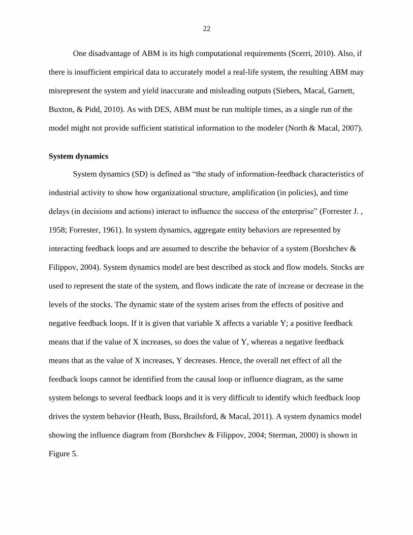
drives the system behavior (Heath, Buss, Brailsford, & Macal, 2011). A system dynamics model
showing the influence diagram from (Borshchev & Filippov, 2004; Sterman, 2000) is shown in
Figure 5.

23
Figure 5. A system dynamics model of “product diffusion” in the form of a stock and flow
diagram (Borshchev & Filippov, 2004).
In Figure 5, “Potential Adopters” become “Adopters” at an “Adoption Rate” that depends
upon the rate of promotion of “word of mouth” and through “advertising”. The total “Adoption
Rate” is the sum of “advertising” effectiveness (i.e., the rate at which potential adopters convert
to adopters) and the adoption rate due to “word of mouth” (i.e., the contact rate at which
potential adopters come into contact with the adopters). The main disadvantage of this type
modeling is that items in the individual stocks are indistinguishable. Thus heterogeneous entities
can’t be modeled. In reality, every entity in the system might have different adoption rates due to
“advertisement”. Also, the “word of mouth” adoption rate might differ between two different
adopters. Therefore, aggregating the adopters into one or a reasonably finite number of stocks
can distort the results (Borshchev & Filippov, 2004). Another drawback of system dynamics is
that the structure of the supply chain is predetermined, which is not generally applicable to real
supply chains and especially to RFSCs (Schieritz & Grobler, 2003).
However, SD has advantages if the modeling is to be done at a system level. SD
simulation has been used in supply chain management to support strategic decision making in the
areas of inventory management, demand amplification, supply chain redesign and in
international supply chain management (Angerhofer & Angelides, 2000). System dynamics has
24
also been used to identify effective policies and optimal parameters to make strategic decisions
in a food supply chain (Georgiadis, Vlachos, & Iakovou, 2005). The authors implemented the
developed methodology for transportation capacity planning in a major Greek fast-food
restaurant supply chain. There is often insufficient data available to model manufacturing
systems in detail, and SD can be very useful to support strategic decisions. However, the quality
of the simulation results is inadequate for modeling systems at an operational level (Helal, 2007).
ABM vs DES – A long Controversy
There has been a long controversy in the literature regarding whether ABM can be
modeled as DES models and vice versa, and if there is really a need for both the simulation
methodologies. This section describes this controversy and argues that both of these simulation
methodologies are necessary to model complex supply chains.
ABM and DES are both discrete time simulations. It is possible to model queuing
systems using ABM (Pugh, 2006; Borshchev & Filippov, 2004), but queuing systems of any
significant complexity are difficult to model in the agent-based environment, due to high
computational requirements (Pugh, 2006). Agent actions can be modeled as events in a DES, and
agent interactions can be represented via the arrival, service, and exiting processes. However,
doing so will exponentially increase the number of events in the DES, making the model
inefficient and hard to analyze (Chan, Son, & Macal, 2010).
To compare the two methodologies, DES model and ABM have been developed in
parallel to study the fitting room operations of a retailer in the U.K. The study found that both
models performed equally well but concluded that the DES model was easier to build and
validate than an equivalent ABM (Majid, Aickelin, & Siebers, 2009). The emergent behavior of
an ABM could be incorporated in DES using timed triggers or probabilities, but this requires an

25
iterative approach, with a couple of cycles of using results of one model to improve the other
model. Also, making any significant changes to the modeled system would require updating both
models, thus repeating the iterative movement (Heath, Buss, Brailsford, & Macal, 2011).
There is significant evidence from the literature to support the need for both ABM and
DES. Siebers, et al. (2010) concluded that true ABM in OR doesn’t exist. Therefore, they
developed a hybrid ABM-DES model in which a process-oriented framework was represented
using a DES model, and the passive entities of the DES were replaced by the active agents of the
ABM. Behdani (2012) mentions that DES is appropriate if the focus of the model is on the
logistics of order fulfillment and delivery. However, modeling interactions between the
customers and manufacturers is beyond the fundamental concepts and standard procedures of
discrete event modeling. The author also concluded that although efforts have been made to
include active entities in DES models, if the active entities are required, ABM may be
conceptually more appropriate. Heath et al. (2011) suggests that in DES, once an entitiy begins
processing, it is difficult to interrupt that processing if there are any changes in the environment
after the processing has begun. Also, it is easy to model queuing behavior as well as the
processing of entities that require multiple sources in DES. In some ABM toolkits, it is really
difficult to model this type of behavior (Heath, Dolk, Lappi, Sheldon, & Yu, 2009). The authors
recommend using a two-model approach, rather than trying to construct a single model with both
ABM and DES attributes. In this approach two models are built using two different software
packages (one for DES and the other for ABM), and use these models to inform each other. This
will enable the modeler to leverage the strength of both modeling paradigms. Table 1
summarizes the important differences between the three simulation techniques described above
in relation to a supply chain context ( (Behdani, 2012; Heath, Buss, Brailsford, & Macal, 2011;

26
Schieritz & Grobler, 2003; Helal, 2007; Moradi, Nasirzadeh, & Golkhoo, 2015; Sumari, Ibrahim,
Zakaria, & Ab Hamid, 2013).
Table 1. Comparison of three most popular simulation techniques in supply chain management.
Basis of
comparison
System Dynamics Discrete Event
Simulation
Agent Based
Simulation
Comments
1 Purpose Strategic decision
making at a system
level
Optimize, precise
prediction and
comparing
scenarios
Study emergent
behavior of the
system due to
interacting
autonmous agents
2 Problem scope Strategic level as it
is a top down
approach and
modelling is done
at a system level
Operational level
to capture more
details
Operational level
to capture more
details
SD is used mainly at strategic
level to evaluate policies,
whereas DES and ABM is used
for decision making at
operational level
3 Modeling approach Top down
approach
Bottom up
approach
Bottom up
approach
4 Unit of analysis Structure of the
system
Rules assigned to
entitities
Rules assigned to
agents
5 Model components Feedback loops Queues, activities
and processes
Agents and
environment
6 Control
parameters
Flow rate Time of queue Agents interaction
7 Nature of model Deterministic Stochastic Stochastic
8 Amount of data
required
Low High High That’s why DES and ABM are
more accurate, but if there is
inadequate data and the
decisions are to be made at
the system level, SD is
preferred over DES and ABM.
9 Accuracy Low High High Accuracy is low in SD due to
aggregate behavior of entities
10 Predictabality Low High High
11 Structure of the
system
Fixed Not fixed (Process
is fixed)
Not fixed
12 Hetrogenity No distinctive
entities, aggragate
behavior of the
entities is assumed
Distinctive and
hetrogenous
entities
Distinctive and
hetrogenous
entities
SD has no micro level entities,
whereas in DES microlevel
entities are passive and in ABS
microlevel entities are active
agents which interacts with
each other and the
environment (Strength of ABM
and DES over SD)13 Entitiy behavior Active entities Passive entities Active -
autonomous
entities (agents)
Strength of ABS over DES

27
Table 1. (Continued)
Basis of
comparison
System Dynamics Discrete Event
Simulation
Agent Based
Simulation
Comments
14 Interactions Average value of
interactions are
modeled
Interactions
possible at physical
level (for example:
manufacturing
lines connected to
the warehouse)
Interactions
possible at physical
and social level
(social level
includes formal
and informal
interactions among
the agents)
Strength of ABS over DES and
SD
15 Adaptiveness No adaptiveness at
individual level
No adaptiveness at
individual level
Adaptiveness at
individual level
Memories of entities and
agents to learn and adapt their
behaviors based on experience
16 Time steps Continuous Discrete Discrete
17 Nestedness Hard to present Not usually
presented
Straightforward to
present
18 Emergence Debatable because
lack of modeling of
one system lvel
Debatable because
of pre-defined
system properties
Capable to capture
because modeling
is done at two
distinct level, agent
and environment
The system level behavior in a
complex system which
emergence from the behavior
of individual components and
their interactions
19 Self-organizaton Hard to capture
due to aggregate
behavior of the
entities
Hard to capture
due to passive
entities
Capable to captue
because of
modeling
autonomous
agents
Self organization means
emergence of the system due
to only local interactions
among the agents and entities
in the system and without any
presence of external factors
20 Co-evolution Hard to capture as
system structure is
fixed
Hard to capture as
the processes are
fixed
Capable as the
network structure
is modified by
agents interactions
Co-evolution corresponds to
change in the states of entities
and agents due to their
adaptive nature along with
change in the physical
components of the system21 Path dependency Debatable as no
explicit
consideration of
history to
determine future
state
Debatable as no
explicit
consideration of
history to
determine future
state
Capable to capture
because current
and future state
can be explicitly
defined based on
system history
Path dependency means,
current and future states and
decision in a complex system
depend upon previous states,
actions or decisions, rather
thean simple on current
conditions 22 Animations and
graphics
System behavior is
difficult to be
identified from
graphics and
animations
Easy to understand
with the help of
animations and
graphics
System behavior is
difficult to be
identified from
graphics and
animations
Graphical representation
sometimes helps the modeler
to verify and validate the
model
23 Experimentation in
the model
Experimentation
done by changing
the system
structure
Experimentaion
done by changing
the process
structure
Experimentation
done by changing
the agent rules and
system structure

28
Hybrid Simulation
To integrate human decision making and behavior with the capabilities of DES,
researchers have combined DES with ABM to form hybrid simulations (Huanhuan, Yuelin, &
Meilin, 2013). Hybrid simulation enables researchers to leverage each individual methodology’s
strengths and analyze systems that could not be realistically modeled using a single approach
(Powell & Mustafee, 2014; Zulkepli, Eldabi, & Mustafee, 2012). The literature suggests that
hybrid simulation modeling is a growing trend, but the concept is still in the early stages of
development (Eldabi, et al., 2008).
Hybrid simulation has been used to simulate transportation evacuation and disaster
response systems (Zhang, Chan, & Ukkusuri, 2011). ABM was integrated with DES to simulate
the movement of people in a theme park, in which people interact with other people and objects
in the park to reach their destination (Dubiel & Tsimhoni, 2005). A hybrid (DES-ABM) model
of patients in a clinic in the United Kingdom incorporated patient interactions into the clinic’s
fundamental queuing problem (Viana, Rossiter, Channon, Brailsford, & Lotery, 2012; Brailsford,
Viana, Rossiter, Channon, & Lotery, 2013). The authors mention that in order to incorporate the
social care side (i.e., patient interactions) with the fundamental queuing problem of the clinic,
using a hybrid methodology was a desirable option. This enabled them to realistically capture the
actual system, which could not have been easily done using a single simulation technique. A
similar model for the treatment of chlamydia was developed (Viana, 2011). In this system, many
patients book appointments, but due to long wait times, patients may leave the clinic without
getting tested, and the infection spreads. This further increases the proportion of infected people
in the community and the demand for the clinic. In this case the queuing behavior is captured by
a DES model (built using Simul8), and the effect of spreading infection leading to increased
demand of clinic is captured by an SD model (built using Vensim). Although hybrid simulations

29
leverage the strengths of different simulation methodologies, they require much more effort to
develop and are computationally difficult to execute (Heath, Buss, Brailsford, & Macal, 2011;
Moradi, Nasirzadeh, & Golkhoo, 2015). Also, the increased complexity that results from using
multiple methodologies means that hybrid models are difficult to validate, since simpler models
are generally easier to validate (Barton, Bryan, & Robinson, 2004).
Execution strategies for hybrid simulation
Mustafee, et al. (2015) mention three different execution strategies for hybrid simulation
models. The first strategy involves two different modeling packages for different simulation
techniques, with the output of one serving as the input to the other, and the operation is done
manually. This methodology has been applied by (Zulkepli, Eldabi, & Mustafee, 2012) to
develop and run a hybrid DES-SD model of an Integrated Care system in healthcare. The second
strategy also involves two modeling packages, but the integration between them is automated.
Examples include the use of Excel to link a DES-SD model (Viana, Brailsford, Harindra, &
Harper, 2014) and the use of a distributed simulation system to link an ABM-DES model
(Mustafee, Sahnoun, Smart, Baudry, & Louis, 2015). The third approach to hybrid simulation
model execution is through the use of a single modeling package that supports multiple modeling
paradigms. For example, the hospital workflow model (a combination of ABM, DES, and SD
methodologies) and an ABM-DES model of a material handling process in an assembly line
were both developed and run using AnyLogic (Djanatliev & German, 2013; Hao & Shen, 2008).
Empirical Simulation Models
The use of empirical research methods in operations management supports the
development of theory (Filippini, 1997). Empirical research also provides a strong foundation for

30
making realistic assumptions in simulation modeling and enables a better understanding of the
system under study (Flynn, Sakakibara, Schroeder, Bates, & Flynn, 1990). Although much of the
existing research on ABM is theoretical and abstract, there has been an increasing trend of
combining ABM with empirical data (Janssen & Ostrom, 2006). Providing input values to ABM
variables and parameters through social survey data demonstrates a strong empirical foundation
for the development of these models (Sopha, Klöckner, & Hertwich, 2013). In particular,
integrating ABM with empirical research can lead to a better representation of the human
decision-making process. For example, an ABM was developed to study the diffusion of water-
saving innovations in households in Southern Germany (Schwarz & Ernst, 2009). The
information on the household agents was gathered through a telephonic survey. Brown and
Robinson (2006) developed an empirical ABM to study the selection of residential locations
within an urban system in southeastern Michigan. The authors used a survey to collect
information on residents’ preferences, and the survey data was used to inform the ABM.
Evaluating RFSC Performance
Many analytical methods have been adopted to evaluate RFSCs. Route and load
optimization methodologies using analytical software (e.g., GIS and Route LogiX) have been
proposed for regional food distribution systems (Bosona & Gebresenbet, 2011; Bosona T. ,
Gebresenbet, Nordmark, & Ljungberg, 2011). Craven, Mittal and Krejci (2016) proposed a
coordinated transportation system among the four food hubs in Iowa to help them better meet the
supply and demand of local food and reduce their overall distribution costs. Nordmark, et al.
(2012) used empirical and analytical methods to study the impact of internet-based systems and
evaluate environmental and economic impacts due to transportation optimization in local food

31
supply chains. Demir and Demir (2014) developed an integer programming model to evaluate
the transportation performance of 62 organic fresh produce farmers in Istanbul.
Using simulation is cost-effective and can enable useful investigations and system
improvement implementations without experimenting with the real world systems (Schieritz &
Grobler, 2003; Towill, Naim, & Wikner, 1992). However, a literature survey done by (Soysal,
Bloemhof-Ruwaard, Meuwissen, & van der Vorst, 2012), suggests that very few simulation
models have been developed in sustainable food logistics management. Jansen, et al. (2001)
developed a DES model to analyze the implementation of a multi-compartment distribution
system in a catering supply chain in the Netherlands. DES has been used to evaluate the
performance of a supply chain for chilled food products (Van der Vorst, Beulens and van Beek
2000), as well as comparing different transport modes in terms of logistics cost, energy use, CO2
emissions, and product quality decay (Van der Vorst, Tromp and Zee 2009). Vorst (1998)
developed a computer simulation model to study the effect of uncertanitites on food supply chain
performance. Krejci and Beamon (2015) used ABM to study the impacts of the farmer
coordination on the emergence of different types of RFSC structures over time. Their model
captures price negotiations between farmer and distributor agents. Bora and Krejci (2015) used
ABM to evaluate various supplier selection policies in RFSCs.
We are unaware of any simulation models in the existing literature that address RFSC
management policies. This thesis proposes and demonstrates the need for hybrid simulation to
evaluate RFSCs through the development of an empirically-based hybrid simulation model to
study the inbound logistics operations of a regional food hub in Iowa.

32
References
Angerhofer, B. J., & Angelides, M. C. (2000). System dynamics modelling in supply chain
management: research review. Proceedings of the 2000 Winter Simulation Conference (pp.
342-351). IEEE.
Barton, P., Bryan, S., & Robinson, S. (2004). Modelling in the economic evaluation of health care:
selecting the appropriate approach. Journal of health service research policy, 9(2), 110-
118.
Beamon, B. M. (1998). Supply chain design and analysis: Models and methods. International
journal of production economics, 55(3), 281-294.
Behdani, B. (2012). Evaluation of paradigms for modeling supply chains as complex socio-
technical systems. Proceedings of the 2012 Winter Simulation Conference (pp. 1-15).
IEEE.
Bora, H., & Krejci, C. C. (2015). Multi-agent simulation modelling of supplier selection for local
food systems. Industrial and Systems Engineering Research Sessions (ISERC).
Borshchev, A., & Filippov, A. (2004). From system dynamics and discrete event to practical agent
based modeling: reasons, techniques, tools. Proceedings of the 22nd international
conference of the system dynamics society, 22.
Bosona, T. G., & Gebresenbet, G. (2011). Cluster building and logistics network integration of
local food supply chain. Biosystems engineering. Biosystems engineering, 108(4), 293-
302.
Bosona, T., Gebresenbet, G., Nordmark, I., & Ljungberg, D. (2011). Box-scheme based delivery
system of locally produced organic food: evaluation of logistics performance. Journal of
Service Science and Management, 4(03), 357.
Brailsford, S. (2014). Discrete-event simulation is alive and kicking! Journal of Simulation, 8(1),
1-8.
Brailsford, S. C., Viana, J., Rossiter, S., Channon, A., & Lotery, A. J. (2013). Hybrid simulation
for health and social care: The way forward, or more trouble than it's worth? In Proceedings
of the 2013 Winter Simulation Conference (pp. 258-269). IEEE.
Brown, D. G., & Robinson, D. T. (2006). Effects of heterogeneity in residential preferences on an
agent-based model of urban sprawl. Ecology and society, 11(1), 46.
Chan, W. K., Son, Y. J., & Macal, C. M. (2010). Agent-based simulation tutorial-simulation of
emergent behavior and differences between agent-based simulation and discrete-event
simulation. Proceedings of the 2010 Winter Simulation Conference, (pp. 135-150).

33
Chang, Y., & Makatsoris, H. (2001). Supply chain modeling using simulation. International
Journal of simulation, 2(1), 24-30.
Chopra, S., & Meindl, P. (2007). Supply chain management. Strategy, planning & operation.
Gabler.
Craven, T., Mittal, A., & Krejci, C. C. (2016). Effective Coordination in Regional Food Supply
Chains. Paper to be presented at the 2016 Industrial & Systems Engineering Research
Conference. Anaheim: IIE.
Davidsson, P., Henesey, L., Ramstedt, L., Törnquist, J., & Wernstedt, F. (2005). An analysis of
agent-based approaches to transport logistics. Transportation Research part C: emerging
technologies, 13(4), 255-271.
Demir, A. Y., & Demir, M. C. (2014). Vehicle Routing Solution Reduces Transportation Costs for
Organic Farmers Serving the Domestic Market in Turkey. International Journal of
Applied, 4(6).
Deshpande, P. J., Yalcin, A., Zayas-Castro, J., & Herrera, L. E. (2007). Simulating less-than-
truckload terminal operations. Benchmarking: An international journal, 14(1), 92-101.
Djanatliev, A., & German, R. (2013). Prospective healthcare decision-making by combined system
dynamics, discrete-event and agent-based simulation. Proceedings of the 2013 Winter
Simulation Conference (pp. 270-281). IEEE.
Dubiel, B., & Tsimhoni, O. (2005). Integrating agent based modeling into a discrete event
simulation. Proceedings of the 2005 Winter Simulation Conference (pp. 9 - pp). IEEE.
Eldabi, T., Jahangirian, M., Naseer, A., Stergioulas, L., Young, T., & Mustafee, N. (2008). A
survey of simulation techniques in commerce and defence. Proceedings of the 4th
Simulation Workshop.
Filippini, R. (1997). Operations management research: some reflections on evolution, models and
empirical studies in OM. International Journal of Operations & Production Management,
17(7), 655-670.
Flynn, B. B., Sakakibara, S., Schroeder, R. G., Bates, K. A., & Flynn, E. J. (1990). Empirical
research methods in operations management. Journal of operations management, 9(2),
250-284.
Forrester. (1961). Industrial Dynamics. MIT Press.
Forrester, J. (1958). Industrial Dynamics: A Major Breakthrough for Decision Makers. Harvard
Business Review, 36(4), 37-66.
Georgiadis, P., Vlachos, D., & Iakovou, E. (2005). A system dynamics modeling framework for
the strategic supply chain management of food chains. Journal of food engineering, 70(3),
351-364.

34
Hao, Q., & Shen, W. (2008). Implementing a hybrid simulation model for a Kanban-based material
handling system. Robotics and Computer-Integrated Manufacturing, 24(5), 635-646.
Heath, S. K., Buss, A., Brailsford, S. C., & Macal, C. M. (2011). Cross-paradigm simulation
modeling: challenges and successes. In Proceedings of the 2011 Winter Simulation
Conference, (pp. 2788-2802).
Heath, S. K., Dolk, D., Lappi, E., Sheldon, B., & Yu, L. (2009). Investigating the use of simulation
tools for mass casualty disaster response. Proceedings and Bulletin of the International
Data Farming Community, 6, pp. 22-25.
Helal, M. R. (2007). A methodology for integrating and synchronizing the system dynamics and
discrete event simulation paradigms. In Proceedings of the 25th international conference
of the system dynamics society, 3(3), pp. 1-24.
Huanhuan, W., Yuelin, Z., & Meilin, Z. (2013). A framework for integrating discrete event
simulation with agent-based modeling. Innovation Management and Industrial
Engineering (ICIII), 2013 6th International Conference. 3, pp. 176-180. IEEE.
Jansen, D. R., Van Weert, A., Beulens, A. J., & Huirne, R. B. (2001). Simulation model of multi-
compartment distribution in the catering supply chain. European Journal of Operational
Research, 133(1), 210-224.
Janssen, M. A., & Ostrom, E. (2006). Empirically based, agent-based models. Ecology and Society,
11(2), 37.
Knaak, N. K. (2006). An agent-based simulation tool for modelling sustainable logistics systems.
Proceedings of the iEMSs Third Biennial Meeting: Summit on Environmental Modelling
and Software. . International Environmental Modelling and Software Society.
Krejci, C., & Beamon, B. (2015). Impacts of Farmer Coordination Decisions on Food Supply
Chain Structure. Journal of Artificial Societies and Social Simulation, 18(2), 19.
Lee, Y. H., Cho, M. K., Kim, S. J., & Kim, Y. B. (2002). Supply chain simulation with discrete–
continuous combined modeling. Computers & Industrial Engineering, 43(1), 375-392.
Liong, C. Y., & Loo, C. S. (2009). A simulation study of warehouse loading and unloading systems
using Arena. Journal of Quality Measurement and Analysis, 5(2), 45-56.
Majid, M. A., Aickelin, U., & Siebers, P. O. (2009). Comparing simulation output accuracy of
discrete event and agent based models: a quantitative approach. Proceedings of the 2009
Summer Computer Simulation Conference (pp. 177-184). Society for Modeling &
Simulation International.
Moradi, S., Nasirzadeh, F., & Golkhoo, F. (2015). A hybrid SD–DES simulation approach to
model construction projects. Construction Innovation, 15(1), 66-83.

35
Mustafee, N., Sahnoun, M. H., Smart, A. G., Baudry, D., & Louis, A. (2015). Investigating
Execution Strategies for Hybrid Models developed using Multiple M&S Methodologies.
2015 Sprind SImulation Multi-Conference.
Nordmark, I., Ljungberg, D., Gebresenbet, G., Bosona, T., & Jüriado, R. (2012). Integrated
logistics network for the supply chain of locally produced food, Part II: Assessment of E-
trade, economic benefit and environmental impact. Journal of Service Science and
Management, 5(3), 249-262.
North, M. J., & Macal, C. M. (2007). Managing business complexity: discovering strategic
solutions with agent-based modeling and simulation. Oxford University Press.
Owen, C. (2013). Selection of simulation tools for improving supply chain performance. Doctoral
dissertation. Aston University.
Powell, J., & Mustafee, N. (2014). Soft or approaches in problem formulation stage of a hybrid
M&S study. Proceedings of the 2014 Winter Simulation Conference (pp. 1664-1675).
IEEE Press.
Pugh, G. A. (2006). Agent-Based Simulation of discrete-event systems. Proceedings of the 2006
Illinois-Indiana and North Central Joint Section Conferences.
Scerri, D. D. (2010). An architecture for modular distributed simulation with agent-based models.
Proceedings of the 9th International Conference on Autonomous Agents and Multiagent
Systems, 1, pp. 541-548.
Schieritz, N., & Grobler, A. (2003). Emergent structures in supply chains-a study integrating
agent-based and system dynamics modeling. In System Sciences, 2003. Proceedings of the
36th Annual Hawaii International Conference (pp. 9-pp). IEEE.
Schwarz, N., & Ernst, A. (2009). Agent-based modeling of the diffusion of environmental
innovations—an empirical approach. Technological forecasting and social change, 76(4),
497-511.
Siebers, P. O., Macal, C. M., Garnett, J., Buxton, D., & Pidd, M. (2010). Discrete-event simulation
is dead, long live agent-based simulation! Journal of Simulation, 4(3), 204-210.
Sopha, B. M., Klöckner, C. A., & Hertwich, E. G. (2013). Adoption and diffusion of heating
systems in Norway: coupling agent-based modeling with empirical research.
Environmental Innovation and Societal Transitions, 8, 42-61.
Soysal, M., Bloemhof-Ruwaard, J. M., Meuwissen, M. P., & van der Vorst, J. G. (2012). A review
on quantitative models for sustainable food logistics management. International Journal
on Food System Dynamics, 3(2), 136-155.
Sterman, J. (2000). Business Dynamics: Systems Thinking and Modeling for a Complex World.
McGraw Hill.

36
Sumari, S., Ibrahim, R., Zakaria, N. H., & Ab Hamid, A. H. (2013). Comparing three simulation
model using taxonomy: system dynamic simulation, discrete event simulation and agent
based simulation. International Journal of Management Excellence, 1(3), 54-59.
Terzi, S., & Cavalieri, S. (2004). Simulation in the supply chain context. Computers in industry,
53(1), 3-16.
Towill, D. R., Naim, M. M., & Wikner, J. (1992). Industrial dynamics simulation models in the
design of supply chains. International Journal of Physial Distribution & Logistics
Management, 22(5), 3-13.
Van der Vorst, J. G., Beulens, A. J., & van Beek, P. (2000). Modelling and simulating multi-
echelon food systems. European Journal of Operational Research, 122(2), 354-366.
Van der Vorst, J. G., Tromp, S. O., & Zee, D. J. (2009). Simulation modelling for food supply
chain redesign : integrated decision making on product quality, sustainability and logistics.
International Journal of Production Research, 47(23), 6611- 6631.
Viana, J. (2011). The development of a combined simulation approach in a sexual health context
- combining discrete event and system dynamics simulation to form a composite model.
Doctrol dissertation. University of Southampton.
Viana, J., Brailsford, S. C., Harindra, V., & Harper, P. R. (2014). Combining discrete-event
simulation and system dynamics in a healthcare setting: A composite model for Chlamydia
infection. European Journal of Operational Research, 237(1), 196-206.
Viana, J., Rossiter, S., Channon, A. A., Brailsford, S. C., & Lotery, A. (2012). A multi-paradigm,
whole system view of health and social care for age-related macular degeneration.
Proceedings of the 2012 Winter Simulation Conference (p. 95). IEEE.
Vorst, J. G. (1998). Supply chain management in food chains: Improving performance by reducing
uncertainty. International Transactions in Operational Research, 5(6), 487-499.
Zhang, B., Chan, W. K., & Ukkusuri, S. V. (2011). Agent-based discrete-event hybrid space
modeling approach for transportation evacuation simulation. Proceedings of the 2011
Winter Simulation Conference (pp. 199-209). IEEE.
Zulkepli, J., Eldabi, T., & Mustafee, N. (2012). Hybrid simulation for modelling large systems:
An example of integrated care model. Proceedings of the 2012 Winter Simulation
Conference (pp. 1-12). IEEE.

37
CHAPTER 3
HYBRID SIMULATION MODEL
This section describes a hybrid simulation model of inbound operations at a regional food
hub in Iowa. The food hub operates as an online grocery store and sell products directly to its
customers. The food hub has two order cycles per month. An order cycle consists of the four
stages described below:
1) Inventory listing – Producers list the products that they are willing to sell in the current
order cycle on the food hub webpage.
2) Shopping period – Every order cycle has a “cart open” period of six days, in the week
prior to the distribution week. Throughout this period, food hub members may add
products to their online shopping carts via the food hub webpage.
3) Receiving process – As per the customer orders, each producer delivers products to the
food hub warehouse. The producers may either deliver their products on the day prior to
the distribution day (i.e., the day that products are distributed to customers) or on the
distribution day. The volunteers at the food hub inspect the products to ensure that the
delivered items and quantities match the orders, and that the quality of the products is
acceptable. The volunteers then place the products in the appropriate storage locations by
product category.
4) Delivery process – After all of the products have been received, the food hub sorts and
delivers the products to multiple distribution points throughout central Iowa, where the
customers pick up their orders.

38
The timeline diagram of the food hub describing all four stages of an order cycle is
shown in Figure 6.
Figure 6. Timeline diagram describing four stages in an order cycle at the food hub.
The hybrid simulation model described in this section is focused on the receiving process
at the food hub, which includes the arrival of the food hub producers to the hub, the quantity
check and quality inspection by the volunteers, and the placement of the goods in storage. The
food hub considered in this study has enabled its producers to schedule the dates and times of
their deliveries via an online on the day prior to the distribution day and three on the distribution
day) for their delivery to the food hub. However, as described in Chapter 1, small and mid-sized
producers highly value their autonomy. As a result, only approximately 25% of the producers
schedule their deliveries in advance, and only a few of those who use the schedule actually show
up in their chosen time slot (Huber, 2015). Unscheduled deliveries result in speeding up the
receiving process by the food hub personnel due to many producers arriving at the same time,
thus leaving less time for quality checks and inventory put-away. This increases the likelihood of
errors in product placement in storage locations and leads to customer dissatisfaction, due to
poor quality of products, or wrong delivery.

39
This thesis describes a hybrid simulation (DES-ABM) model that employs an ABM to
capture food hub producers’ delivery scheduling decisions and behaviors and a DES model to
represent the food hub’s receiving process, with the DES model providing feedback to the ABM.
These models run in a sequence as shown in Figure 7. In Stage 1, the ABM (created using
NetLogo 5.1.0) determines the producer agents’ scheduling decisions and generates the arrival
times of the producers at the food hub warehouse according to these decisions. These arrival
times become the input to Stage 2, which is a DES model (developed using Arena 14.7) of
inbound operations at the warehouse. This model generates the queue time of each producer as
he waits his turn to be served by a volunteer for receiving. The queue time serves as an input to
the producer agents in the ABM. The data exchange between these two separate models is
performed manually, using the read/write functions of both software platforms.
Figure 7. Hybrid simulation (ABM-DES) model overview.
Agent-Based Model
As described in Chapter 1, agent-based modeling (ABM) is well-suited to modeling
heterogeneous components in a supply chain. In a regional food supply chain that is
intermediated by a food hub, these components may include producers, the food hub, consumers,
and the volunteers who work at the food hub. However, in the ABM described in this thesis, only
one of these components is represented as an agent: the producers.
40
This ABM is used to analyze producers’ decisions to schedule their deliveries before
arriving to the food hub. These decisions are often influenced by multiple factors. For example,
producers often like to combine multiple deliveries in the same area, coordinate their deliveries
with other activities, and coordinate and share deliveries with other producers. The decision to
schedule is also subject to the producers’ desire to maintain their autonomy and flexibility.
Small and mid-sized producers associated with the food hub (i.e., farmers) are known to highly
value their autonomy, and they are often willing to make significant sacrifices to maintain it
(Krejci & Beamon, 2015). However, one of the main incentives for selling products through a
food hub is the convenience of avoiding multiple direct-to-consumer transactions.
This thesis describes an empirical ABM that was developed using data from a survey of
the producers associated with the Iowa Food Cooperative (a food hub based in Des Moines,
Iowa) and informal interviews with the food hub manager. The producer survey questionnaire
targets behavioral components that include different factors affecting producers’ decisions to
schedule their deliveries. The detailed survey questionnaire and its explanation is provided in
Appendix A.
Parameterization of the ABM
The main strength of ABM is its ability to implement human decision-making processes.
The agent attributes and behavioral response functions in an ABM require knowledge from
empirical sources (Smajgl, Brown, Valbuena, & Huigen, 2011). In the development of an
empirical ABM, two fundamental steps are required: development of appropriate behavioral
categories, and scaling the real-world sample to the whole ABM population level. The
population size (i.e., the total number of agents in the ABM) can be anywhere from 20 to many
41
millions, and therefore it becomes necessary to collect empirical data from a sample of the real-
world population, which will represent the agents in the ABM (Smajgl, Brown, Valbuena, &
Huigen, 2011). Therefore, the first step in the parameterization framework includes collecting
the empirical data from the sample of population under study. However, it is important that the
agent population appropriately reflects the actual heterogeneity of the real-world objects that it
represents (Brown & Robinson, 2006). In order to identify the potential factors that affect
producers’ decision to schedule their deliveries, the relevant literature (including journal articles,
case studies published by the U.S. Department of Agriculture and the National Good Food
Network, and manuals published by food hubs in United States) was reviewed, and informal
interviews with two subject matter experts (i.e., food hub managers in Iowa) were conducted
(Huber, 2015; Grimm, 2015). This was followed by a survey of 25 producers, which was
conducted during the delivery process of one of the order cycles at the Iowa Food Cooperative.
Social surveys can serve as the source of information about the heterogeneity present in agents
that are being represented in ABM, provided that the survey questions relate directly to the agent
attributes in the model (Brown & Robinson, 2006). Due to missing values of key parameters for
one of the respondents, the responses of 24 of these producers were used to develop the
empirical ABM. The survey data was used to develop producer agent attributes, thereby
providing input parameters for the simulation.
Based on the literature and the discussions with the food hub managers, six factors were
initially identified as the potential reasons which might affect producers’ decisions to schedule
their deliveries before arriving to the food hub:
1) Producers may combine their deliveries with other activities and other deliveries in the
area near the food hub.

42
2) Producers may combine their deliveries with other producers located near their farm.
3) Producers may be affected by their harvesting schedule, if they harvest on the day of
delivery to the food hub.
4) Producers may value flexibility in delivery times to avoid placing any constraints on their
schedules.
5) Access to the internet (which is required to schedule a delivery) may be inconvenient for
a producer.
6) Producers may value reductions in in queue time at the food hub while waiting for
service from volunteers.
These factors informed the design of the producer survey. The objective of the survey
was to gather information on how the six factors described above impact producers’ scheduling
decision. The survey also consisted of questions related to producers’ current level of satisfaction
of doing business with the food hub, their geographical locations, how their behavior to schedule
will change if the food hub provides certain incentives and other potential factors which are not
listed in the survey but play a significant role in their scheduling decision. At the end, every
producer was asked to rank all the factors (including those when food hub provides incentives to
the producers for scheduling the delivery) in the decreasing order of their importance in their
scheduling decision.
All the survey respondents were producers associated with the food hub and all but one
were aware that the food hub gives an option to schedule their delivery online. Two of the six
factors that were hypothesized to affect producers’ delivery scheduling decisions (internet access
and combining deliveries with other producers) were rarely mentioned by the surveyed
producers. Therefore, these two factors were removed from further analysis. Some of the other
43
factors which came from the responses that affected producers’ scheduling decision and were not
included in the producer survey included weather conditions, ignorance, volunteering at the food
hub, delivering freshest products to the customers and family commitments. We have not
considered these factors in our model as they were not applicable on all the producer population.
The detailed survey results corresponding to different attributes of the ABM and DES models
have been included in the respective model descriptions.
The second step in the ABM parameterization framework involves scaling up the
empirical data to the entire population of agents. To accomplish this, cluster analysis was
performed on the survey data to identify sample agents with similar behavioral patterns (Yim &
Ramdeena, 2015). Only those variables associated with the behavioral attributes of agents in the
ABM were considered in the cluster analysis (Sopha, Klöckner, & Hertwich, 2013). Behavioral
attributes were derived from the producers’ responses to the following survey questions, where
the response was given on a 5-point Likert scale (1 as “not likely” and 5 as “highly likely”).
1) How likely is it that combining your deliveries with other activities and other deliveries
in the area near the food hub affects your decision to schedule the delivery?
2) How likely is it that your harvesting and packing schedule affects your decision to
schedule the delivery?
3) On scale of 1 to 5 (1 is “least satisfied” and 5 as “most satisfied”) what will be your
satisfaction level for the different waiting times to have your products inspected and
checked in by the IFC volunteers? (Refer Appendix A, question number 9, for the
different waiting times included in the survey)

44
4) If the food hub offers you a priority delivery option (i.e. go to the front of the line for
receiving) as an incentive to schedule, how likely is it that you would be scheduling your
delivery?
5) How will your decision to schedule the delivery change for the different monetary
incentive levels provided by the food hub? (Refer Appendix A, question number 14, for
the different monetary incentive levels included in the survey)
6) If you interact with other producers, how often do you share the experiences you have
with the food hub?
Hierarchical clustering analysis (Ward’s Method) was used to identify different clusters
(Punj & Stewart, 1983; Krejci, Stone, Dorneich, & Gilbert, 2015). The sample data was not
standardized before clustering, since all responses were on a same scale. Squared Euclidean
distance was used to generate the agglomerative schedule (Appendix B) to determine the
coefficient values (i.e., the distance between two combined clusters) at each stage of hierarchical
clustering. The increase in coefficient values indicates that the clusters that are combined at any
given stage are more heterogeneous than the previous combinations (Yim & Ramdeena, 2015).
The agglomerative schedule shows that the first notable increase in the coefficient value occurs
at stage 20. Therefore the 24 surveyed producers were grouped into four clusters and were
identified from a unique producer id by visually inspecting the dendrogram as shown in Figure 8.
Table 2 provides a summary of the responses to the six behavioral survey questions for
each of the four clusters. For all the questions, higher the average response values, higher is the
impact, but for the queue time, it is vice versa. If the average value of the responses is 1, then it
has been assumed that the particular factor doesn’t affect producers’ scheduling decision. The

45
value for these average responses for each cluster on the scale of 1 through 5 (1 as “low impact”
and 5 as “impact”) are also indicated in Table 2.
Figure 8. Dendrogram for hierarchical cluster analysis from producers’ survey data.
The producers in Cluster 1 consist of 6 producers. They consider waiting time and
priority delivery option by the food hub as moderately important in their scheduling decision.
However, other activities and deliveries in the area near to the food hub highly drives their

46
decision to schedule the delivery. Harvesting schedule is less important in their decision making.
They would highly consider scheduling the delivery if the food hub provides monetary
incentives and are moderately expressive with respect to sharing their business experiences with
the other food hub producers.
There were 5 producers in Cluster 2. Waiting time at the food hub, priority delivery
option and monetary incentives have moderate impact while other activities in the area have high
impact on their scheduling decision. These producers don’t harvest and pack their products on
the day of the delivery therefore this factor doesn’t impact their scheduling decision at all. They
also don’t communicate much and don’t share their business experiences with the other food hub
producers.
Cluster 3 comprised majority of the respondents. Waiting time moderately affects their
scheduling decision, but if they have been provided with priority queue option for scheduling,
they would highly consider scheduling the delivery. Their scheduling decision is moderately
driven by other deliveries and activities near the food hub area and harvesting schedule
moderately affects their scheduling decision. They would be moderately affected by the
monetary incentives option and the likelihood of sharing their experiences with the other
producers is very less.
Cluster 4 consisted of 4 producers who are highly satisfied with their business with the
food hub. It’s only the waiting time which has a very less impact on their scheduling decision,
and no other factor is responsible in their decision making to schedule the delivery. Their
scheduling behavior will not be affected much due to monetary incentives provided by the food
hub, and they moderately share their positive or negative experiences with the other food hub
producers.

47
Table 2. Behavioral response of four clusters to six attributes.
After clustering, the sample data was translated into behavioral representations for the
whole population using the method called up-scaling. Up-scaling can be done in two ways
(Smajgl, Brown, Valbuena, & Huigen, 2011; Berger & Schreinemachers, 2006):
1) Proportionately – Assumes the sample is representative of the whole population.
Cluster #Queue
time
Priority
delivery
Other
activities
Harvesting
schedule
Monetary
incentive
Sharing
experienceDescription
Cluster 1
(N = 6,
25%)
2.76 3.00 5.00 1.33 4.00 3.33
Queue time at the food hub is moderately
important, priority delivery will moderately impact
their scheduling decision, other activities in the area
highly impact their scheduling decision, harvesting
schedule impact on their scheduling decision is very
less, high impact of monetary incentive on
scheduling decision, likelihood of sharing experience
with other producers is moderate
Cluster 2
(N = 5,
20.8%)
2.37 3.40 4.80 1.00 1.80 2.20
Queue time at the food hub and priority delivery
will moderately impact their scheduling
decision,other activities in the area high impact
their scheduling decision, harvesting schedule
doesn't impact their scheduling decision, moderate
impact of monetary incentive on scheduling
decision, likelihood of sharing experience with other
producers is low
Cluster 3
(N = 9,
37.5%)
3.14 3.89 2.67 3.67 3.00 2.33
Queue time at the food hub is moderately
important, priority delivery will highly impact their
scheduling decision, other activities in the area
moderately impact their scheduling decision,
harvesting schedule moderately impact their
scheduling decision, moderate impact of monetary
incentive on scheduling decision, likelihood of
sharing experience with other producers is low
Cluster 4
(N = 4,
16.7%)
3.50 1.00 1.00 1.00 1.25 3.00
Queue time at the food hub is less important,
priority delivery will not impact their scheduling
decision, other activities in the area doesn't impact
their scheduling decision, harvesting schedule
doesn't impact their scheduling decision, low
impact of monetary incentive on scheduling
decision, likelihood of sharing experience with other
producers is moderate

48
2) Disproportionally – If the sample can’t be assumed to be correct representation of the
whole population, alternative approaches (e.g., Monte Carlo Approach, using census
and GIS data) are employed.
According to its historical sales data, the food hub considered in this study is doing
business with an average of 70 producers per order cycle. The ABM includes 72 producer agents
who are delivering products in every order cycle to the food hub. In order to up-scale the data
from 24 agents to the model population size of 72, the strategy of Schreinemachers et al. (2009)
was adopted, wherein proportional cloning was used to scale the sample data to agent population.
The number of agents in this study was equal to the number of Thai farm households in reality.
They surveyed around a quarter of farm households, and used sampling weights (inverse
probability of selection) to multiply households inside the ABM. Therefore each farm household
appeared about four times in the model. The average of the 24 responses to the six behavioral
questions were up-scaled proportionally by cluster to 72 producer agents in the ABM. Therefore
each cluster appeared three times in the ABM.
ABM Overview
Each of the 72 producer agents in the ABM decides in each time-step whether or not they
will schedule their delivery to the food hub. This decision is informed by factors that are either
1) indirectly related to the food hub or 2) directly related to the food hub. Indirect factors
include the producer’s preference to combine their food hub delivery with other
activities/deliveries in the area and their harvesting schedule. These two factors were ranked as
the most important by the most of the surveyed producers. Each producer agent is assigned a
probability that their decision to schedule their delivery will be affected by these indirect factors

49
in a given time-step. The value of this probability is based on survey responses. The probability
has been assigned based on average value of the responses to these factors within each cluster.
Higher the average response value for a cluster, higher is the probability that the factor will
affect producers’ scheduling decision. It has been assumed that the probability decreases linearly
from 0.8 to 0, if the response value decreases from 5 to 1. 3 out of 24 respondents in the survey
mentioned that they don’t combine their delivery with other deliveries and activities in the area
near the food hub. Figure 9 shows the response of 21 producers in the survey on how their
decision to schedule the delivery gets affected due to this factor. The response was taken on a 5
point Likert scale with 1 as “not likely and 5 as “highly likely”.
Figure 9. Survey data showing the effect of other deliveries and activities in the area near to the
food hub on producers’ decision to schedule the delivery.
Also, 12 out of 24 survey respondents mention that they don’t harvest, pack or label their
products on the day of the delivery. Figure 10 shows the response of the remaining 12 producers’
on how their decision to schedule affects based on their harvesting schedule. The response was
taken on a 5 point Likert scale with 1 as “not likely” and 5 as “highly likely”.

50
Figure 10. Survey data showing the effect of harvesting schedule on producers’ decision to
schedule the delivery.
If a producer’s decision in any given cycle is not affected by these indirect factors, then it
will be influenced by factors that are directly related to the producer’s previous experiences with
the food hub. Specifically, the producer recalls whether he was satisfied with his scheduling
decision in the previous cycle or not. His level of satisfaction is based on two different
components: autonomy (i.e., flexibility in delivery) and convenience. In the model, it is assumed
that the degree of autonomy that a producer experiences depends upon the flexibility he has in
choosing times to deliver goods to the food hub. The level of convenience that a producer agent
experiences depends upon the amount of time that he spends waiting in a queue to receive
service from personnel at the food hub during a delivery.
Every producer has a time preference for delivering their goods to the food hub. The food
hub currently offers 11 one-hour time slots in its online schedule from which the producers can
choose to deliver their goods. These time slots are available between 9:00 am to 5:00 pm on the
day prior to the distribution day and from 8:00 am to 11:00 am on the distribution day in every

51
order cycle. The surveyed producers were asked about their preferences for each of the 11 time
slots, on a scale of 1 to 5, where 5 is most satisfied and 1 is least satisfied. Figure 11 shows the
satisfaction level of the 24 producers surveyed for each of the 11 time slots (1 – 8 represents
receiving day 1 time slots, 9 – 11 represents receiving day 2 time slots). On delivery day 1, slot
number 2 and 6 are highly preferred by the producers to deliver their products. While on delivery
day 2, most of the producers preferred to deliver in the last two time slots.
Figure 11. Satisfaction level of 24 survey respondents to deliver the products in 11 time slots.
It is assumed that this preference does not change over the course of a simulation run.
The slots are assumed to be filled on a first-come-first-served basis, and it is assumed that if a
producer schedules his delivery in a given time slot, he is guaranteed to arrive at the food hub in
that time slot.
The utility that a producer gains from autonomy in each delivery cycle depends upon his
ability to schedule his delivery for his preferred time slot, or better yet, to avoid scheduling

52
altogether. The producer’s utility due to autonomy (UA) is defined on a scale from 0 to1 (where 0
and 1 represent the worst and best possible outcomes, respectively). UA is assigned a value of 1 if
the producer doesn’t schedule his delivery. If a producer decides to schedule his delivery, he will
first check the availability of his most-preferred time slot. If the slot is not full (i.e., it has not
reached its maximum capacity), he will schedule his delivery for this time. If the time slot is full,
he will check for availability in his second most-preferred time slot, and so on, until he is able to
successfully schedule. This is because, all the 24 producers responded in the survey, that if there
most preferred time slot is not available, they will schedule the delivery in their next preferred
time slot. In this case UA decreases linearly from 0.8 to 0, with a value of 0.8 when he get his
most-preferred time slot and 0 if he get his least-preferred time slot.
A producer agent’s utility due to convenience (UC) is a function of producer queue time
(Q) at the food hub. Previous research has shown that an inversely proportional relationship
exists between customer waiting time in queue and customer satisfaction (Davis & Heineke,
1998). However, for producers that are supplying food to regional food hubs, this is not
necessarily the case – for a variety of reasons, not all producers are concerned about the time
they have to wait in queue for their products to get checked in. For example, some of the
producers spend time volunteering at the food hub when they come to drop of their products, so
waiting time in queue doesn’t affect their satisfaction level at all. In the survey, producers were
asked about their satisfaction level on a scale from 1 to 5 for 7 different wait time ranges (where
5 is “most satisfied” and 1 is “least satisfied”). Figure 12 shows the producers’ response to
satisfaction level in the survey corresponding to 7 different ranges of waiting times with 1 as
“least satisfied” and 5 as “most satisfied”.

53
Figure 12. Survey data showing satisfaction level of 24 producers for the 7 different waiting
times range at the food hub.
Utility due to convenience (UC) is defined on a scale of 0.2 to 1. UC is assigned a value of
1 if the producer’s queue time (Q) yields the highest satisfaction level (i.e., 5), and it decreases
linearly to a value of 0.2 if the queue time results in the minimum satisfaction level (i.e., 1).
Figure 13 shows how UC varies for each cluster as the waiting time increases based on the
producers’ responses in the survey.
The overall utility (U) of a producer’s decision is a weighted combination of UA and UC,
given by: U = WAUA + WCUC, where WA and WC are measures of the producer’s relative preference
for autonomy and convenience, respectively. Every producer has a satisfaction threshold, and if
his scheduling decision yields a level of satisfaction that falls below this threshold, he will update
his decision-making strategy in an attempt to improve it. To define this satisfaction in terms of
utility, every producer is assigned a constant threshold utility value (UT) of 0.88, below which a
producer will be dissatisfied. It is calculated by assuming that a producer will be satisfied if he

54
gets at least his most-preferred time slot for scheduling the delivery (UA = 0.8) and his wait time
in the queue is in the range of highest satisfaction level (UC = 1), with WA = 0.6 and WC = 0.4. Table
3 and Table 4 summarize all of the variables and parameters used to describe the state of a producer
agent in the ABM.
Figure 13. Variation of UC vs waiting time for each cluster.
Table 3. ABM variables.
# Variable Description Source Possible values
1 producer_combine_delivery Producer combine his delivery
with other deliveries and
activities in the area in an order
cycle
Producer
survey
1 – if yes
0 – if no
2 producer_harvest Producer harvest on the day of the
delivery in an order cycle
Producer
survey
1 – if yes
0 – if no
3 producer_schedule_delivery Producer decision to schedule the
delivery
ABM 1 – if yes
0 – if no
4 producer_slot_number Time slot number in which the
producer decides to deliver the
products at the food hub
ABM 1 - 8 (day prior to
distribution day)
9 – 11 (on
distribution day)
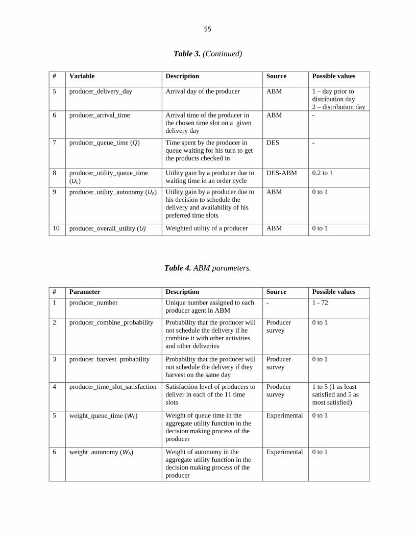
55
Table 3. (Continued)
# Variable Description Source Possible values
5 producer_delivery_day Arrival day of the producer ABM 1 – day prior to
distribution day
2 – distribution day
6 producer_arrival_time Arrival time of the producer in
the chosen time slot on a given
delivery day
ABM -
7 producer_queue_time (Q) Time spent by the producer in
queue waiting for his turn to get
the products checked in
DES -
8 producer_utility_queue_time
(UC)
Utility gain by a producer due to
waiting time in an order cycle
DES-ABM 0.2 to 1
9 producer_utility_autonomy (UA) Utility gain by a producer due to
his decision to schedule the
delivery and availability of his
preferred time slots
ABM 0 to 1
10 producer_overall_utility (U) Weighted utility of a producer ABM 0 to 1
Table 4. ABM parameters.
# Parameter Description Source Possible values
1 producer_number Unique number assigned to each
producer agent in ABM
- 1 - 72
2 producer_combine_probability Probability that the producer will
not schedule the delivery if he
combine it with other activities
and other deliveries
Producer
survey
0 to 1
3 producer_harvest_probability Probability that the producer will
not schedule the delivery if they
harvest on the same day
Producer
survey
0 to 1
4 producer_time_slot_satisfaction Satisfaction level of producers to
deliver in each of the 11 time
slots
Producer
survey
1 to 5 (1 as least
satisfied and 5 as
most satisfied)
5 weight_queue_time (WC) Weight of queue time in the
aggregate utility function in the
decision making process of the
producer
Experimental 0 to 1
6 weight_autonomy (WA) Weight of autonomy in the
aggregate utility function in the
decision making process of the
producer
Experimental 0 to 1

56
Table 4. (Continued)
# Variable Description Source Possible values
7
producer_threshold_utility (UT) Utility below which the producer
will not be satisfied with the
decision
Experimental 0 to 1
8 max_slot_capacity Maximum number of producers
allowed to choose a particular
time slot for scheduling their
delivery
Experimental 6 – 18
Discrete Event Simulation (DES)
DES model captures the activities of the inbound receiving operations in the food hub,
including quality inspection and storage of the goods brought by the producers. The receiving
process of the food hub considered in this thesis is shown in Figure 14. The entities in the DES
model represent the producer agents of the ABM. The four attributes of these entities are the
quantity and the category of the goods they are selling through the food hub in every order cycle,
and their arrival times and waiting times at the food hub. The receiving operations are divided
into four stages in the DES: the arrival of producers at the food hub, queuing for service,
receiving service from the food hub personnel, and exiting the food hub.
Figure 14. Receiving process at the food hub.

57
Producer arrival times that are determined by their scheduling decisions. Upon arrival, if
there are unoccupied receiving personnel available, an arriving producer will immediately be
served; otherwise, the producer will wait in a queue for service. Receiving time is known to be
dependent upon product attributes. For example, milk will have a different receiving time than an
equivalent volume of vegetables/meat. It is necessary for the receiving personnel to count the
quantity and types of milk containers and ensure that these match the values on the producer’s
invoice, as well as inspecting the products’ expiry dates. Vegetable deliveries must be
reconciled to the producer’s invoice, but they also undergo a quality inspection. For example,
every bag of potatoes must be carefully inspected for sprouted or green potatoes, which is a very
time-consuming process. Therefore, quality inspection and product placement time are a function
of both the quantity delivered and the product category. The food hub in this study has
categorized the products sold by its producers into four different categories, which are
summarized in Table 5.
Table 5. Four different types of product categories at the food hub.
Serial # Product Type Description
1 NON Shelf-stable goods
2 FROZ Frozen goods
3 REF Refrigerated goods
4 PLANTS & INVENTORY Plants and dry goods kept as inventory at the food hub
The probability distributions that define the receiving times of products in the DES model
depend on the quantity of goods sold by the producers in each of the four different categories.
The storage strategies adopted by the food hub for each of the four product categories are
described below.

58
NON – Shelf-stable goods
“NON” includes the shelf-stable goods (e.g., salsa, flour, potatoes) sold by the
producers that do not require refrigeration. “NON” goods are stored on shelves in the food hub
warehouse according to customer member identification numbers. Figure 15 schematically
illustrates how the products in the “NON” category of the food hub considered in this study are
stored. The receiving time for “NON” goods depends on the number of customer orders for these
items.
Figure 15. Storage of “NON” goods at the food hub.
FROZ – Frozen goods
“FROZ” includes frozen meat products and other frozen goods (e.g., ice cream), which
are stored in freezers in the food hub warehouse. The goods of each producer are stored at a
unique location in the freezer, which is labeled by the producer’s name. Customer orders are
stored in order of increasing identification number, with the smallest number in the front of the
freezer and largest at the back. Figure 16 shows how “FROZ” products are stored at the food
hub. The receiving time of the frozen goods depends on the number of customer orders within a
producer’s delivery.

59
Figure 16. Storage of “FROZ” goods at the food hub.
REF – Refrigerated goods
“REF” includes all the vegetables, fruit, and dairy products. These items are stored
according to the producer in refrigerators in the food hub warehouse. This storage scheme is
similar to that of the “FROZ” products, but the refrigerated items are not arranged according to
customer identification number. Figure 17 shows the typical storage strategy of “REF” products
for one particular producer at the food hub.
Figure 17. Storage of “REF” goods at the food hub.

60
Plants and inventory goods
The inventory goods are stored in a similar way as that of “REF” products, but as they are
shelf-stable goods they are stored on shelves that are designated to each individual producer. The
plants are also stored according to their producer and are arranged in the order of increasing
customer identification number, as with the “FROZ” products. The overall layout of the food hub
warehouse under study is shown in Figure 18. The layout shows the arrangement of refrigerators,
freezers, dry good shelves, and inventory storage area.
Figure 18. Facility layout of the food hub.

61
Data collection
The volume of products sold in each of the four product categories in the past year was
identified for each of the 24 producers surveyed using the food hub’s sales database. Table 6
describes this data for one order cycle. This data was up-scaled to 72 producer agents using the
hierarchical cluster analysis described previously.
Table 6. Description of data for each of the four product categories.
Serial # Product Type Data Description
1 NON Total number of individual packages brought by the producer labelled
as “NON”
2 FROZ Total number of customers served by a producer
3 REF Total number of individual packages of “REF” products
4 PLANTS & INVENTORY Total counts of plants and inventory goods brought by the producer
The data acquired for receiving time at the food hub per unit of each product type is
based on a time study conducted at the food hub. The time-study was conducted by capturing the
minimum and maximum time taken to receive and store the products for a sample of producers
in each product category. This time-study data was then used to assign the receiving time for
each product category based on the data type as mentioned in Table 5. The range of receiving
times for each of the four product categories is shown in Table 7. In the DES model the receiving
time for per unit in each of the four product categories is drawn from a triangular distribution
with minimum and maximum values as shown in Table 7 and the median value as the average of
these maximum and maximum values.

62
Table 7. Receiving time values for all the three product categories.
Serial # Product Type Unit Minimum time
(minutes)
Maximum
time (minutes)
1 NON Number of orders 0.44 1
2 FROZ Number of customers per producer 0.89 1.18
3 REF Number of orders 0.2 0.3
4 Plants &
Inventory goods
Plants - Number of customers per
producer
0.89 1.18
Inventory goods – Number of orders 0.2 0.3
The number of resources (i.e., food hub personnel) in the DES model is based on the
actual number of volunteers available at the food hub over a period of two days for the receiving
process. On the day prior to the distribution day (delivery window of eight hours), an average of
two volunteers are available; and on the distribution day (delivery window of three hours), six
volunteers are available in the entire time window for the receiving process. Given a producer’s
arrival time, arrival time slot, and quantity and category of products, the DES model outputs the
queue time for each producer. The flowchart of the DES model built using Arena (14.7) is shown
in Figure 19.
Table 8 summarizes the input and output variables used in the DES model. All of the
input variables used in the DES model are either informed by the ABM or derived from the food
hub’s sales database. The parameters used in the DES model related to the receiving process are
summarized in Table 9 and have been derived by the food hub manager based on his expert
knowledge of the food hub’s operations (Huber, 2015).

63
Figure 19. Flowchart of the Arena simulation model.
Table 8. DES variables.
# Variable Description Source Possible values
1 producer_arrival_time Arrival time of the producer at the
food hub as per his time slot
preferences
ABM -
2 producer_scheduling_decision Producer decision if he has scheduled
the delivery in advance or not
ABM 0 – not scheduled
1 - scheduled
3 producer_delivery_day Day of delivery of the producer ABM 1 – delivery day 1
2 – delivery day 2
4 producer_queue_time Time spent by the producer in queue
waiting for his turn to get checked in
DES -
5 average_queue_time_day1 Average waiting time of the producers
on the day prior to the distribution day
DES -
6 average_queue_time_day2 Average waiting time of the producers
on the day of distribution
DES -
7 resource_utilization_day1 Man hour utilization rate for the
receiving process on the day prior to
the distribution day
DES 0 – 100 %
8 resource_utilization_day2 Man hour utilization rate for the
receiving process on the distribution
day
DES 0 – 100 %
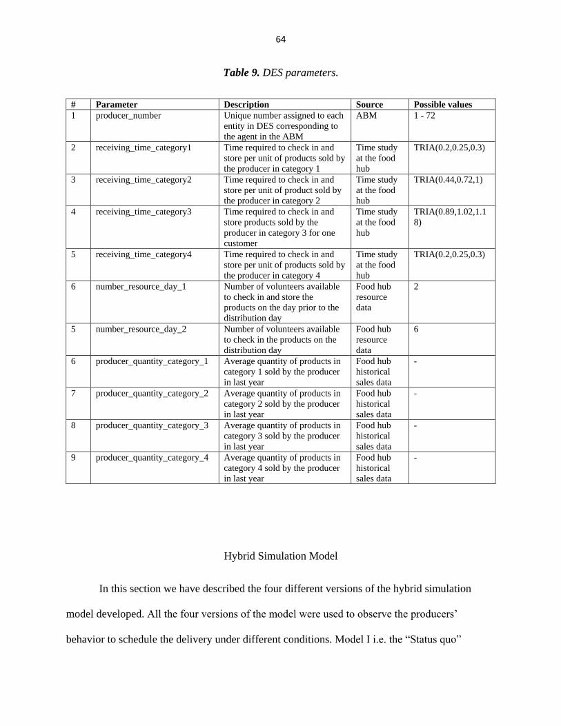
64
Table 9. DES parameters.
# Parameter Description Source Possible values
1 producer_number Unique number assigned to each
entity in DES corresponding to
the agent in the ABM
ABM 1 - 72
2 receiving_time_category1 Time required to check in and
store per unit of products sold by
the producer in category 1
Time study
at the food
hub
TRIA(0.2,0.25,0.3)
3 receiving_time_category2 Time required to check in and
store per unit of product sold by
the producer in category 2
Time study
at the food
hub
TRIA(0.44,0.72,1)
4 receiving_time_category3 Time required to check in and
store products sold by the
producer in category 3 for one
customer
Time study
at the food
hub
TRIA(0.89,1.02,1.1
8)
5 receiving_time_category4 Time required to check in and
store per unit of products sold by
the producer in category 4
Time study
at the food
hub
TRIA(0.2,0.25,0.3)
6 number_resource_day_1 Number of volunteers available
to check in and store the
products on the day prior to the
distribution day
Food hub
resource
data
2
5 number_resource_day_2 Number of volunteers available
to check in the products on the
distribution day
Food hub
resource
data
6
6 producer_quantity_category_1 Average quantity of products in
category 1 sold by the producer
in last year
Food hub
historical
sales data
-
7 producer_quantity_category_2 Average quantity of products in
category 2 sold by the producer
in last year
Food hub
historical
sales data
-
8 producer_quantity_category_3 Average quantity of products in
category 3 sold by the producer
in last year
Food hub
historical
sales data
-
9 producer_quantity_category_4 Average quantity of products in
category 4 sold by the producer
in last year
Food hub
historical
sales data
-
Hybrid Simulation Model
In this section we have described the four different versions of the hybrid simulation
model developed. All the four versions of the model were used to observe the producers’
behavior to schedule the delivery under different conditions. Model I i.e. the “Status quo”

65
represents the current condition at the Iowa Food Cooperative, with producers making their
scheduling decision based on several factors as described above in the ABM. In rest of the three
models, interventions by the food hub have been modeled to encourage producers to schedule the
delivery. In Model II, it has been considered that the food hub will provide an option of priority
queue to the producers who schedule their delivery. In Model III, it has been considered that the
food hub rewards the producers with monetary incentives as well as priority queue for
scheduling their delivery. In Model IV, it has been assumed that the food hub will provide
feedback to the producers on how their inbound operations get affected due to unscheduled
deliveries. The effect of this feedback along with sharing this feedback information among the
producers has been modeled to observe the producers’ overall scheduling decisions.
Model I – Status Quo
The simulation begins with the ABM. In the first delivery cycle, it is assumed that all of
the producers will make their decision to schedule their deliveries based on the two indirect
factors (i.e., their decision to combine the delivery with other activities/other deliveries near the
food hub location and their harvesting schedule). If any one of these factors affects their decision
to schedule the delivery (i.e. not to schedule), it is assumed that the producers will arrive in one
of their most preferred (with satisfaction level of 5) time slots. However, if these two factors are
not affecting producers’ scheduling decision, it is assumed that they will first try to schedule the
delivery in one of their most preferred time slot. If all of their most preferred time slots are not
available to schedule due to capacity restrictions on the time slots, they will try scheduling in
their second most preferred time slot and so on until they are able to successfully schedule the
delivery. The actual producer arrival times to the food hub are assumed to be uniformly

66
distributed within the chosen time slots. These arrival times are written to an output file and
become inputs to the DES.
At this point, the simulation switches to the DES. Upon arrival to the food hub, the
producer (i.e., entity) will either receive service from food hub personnel immediately, or he will
wait for service in the queue. The service time is the time required to receive the product into
inventory, which includes a quantity check, quality inspection, and product placement in storage
which is dependent on the product quantity and category brought by the producer to the food
hub. The producer’s queue time is written to an output file, which becomes an input file to the
ABM. The producer’s queue time (Q) is then used to calculate his utility due to convenience
(UC). Also, as per the producer’s decision to schedule his delivery in the previous cycle, he will
calculate his utility due to autonomy (UA). The producer’s overall utility (U) is then calculated
using the weighted utility function.
From the second order cycle, the producer will first determine his scheduling decision
due to combining delivery with other activities and harvesting schedule. If these factors don’t
affect his decision to schedule, then the producer compares his overall utility (U) of the previous
cycle with the threshold utility (UT). If U is greater than UT, then he will maintain his current
strategy to schedule/not schedule; otherwise, he will reverse his decision.
This process of deciding on a scheduling policy, arriving at the food hub, queueing,
receiving service, and updating the scheduling policy based on different factors and utility
outcomes, occurs for each of the 72 producer agents in every time-step, where one time-step is
equivalent to one two-week delivery cycle for the food hub. The overall process is shown in
Figure 20.

67
Figure 20. ABM- DES model overview (Status Quo).
Food hub interventions
In order to encourage producers to schedule their deliveries, food hub managers should
take corrective actions as necessary in order to improve their inbound operation’s efficiency and
to avoid lost sales due to bad quality or wrong products reaching the customers. In order to
reduce these errors, food hubs can consider encouraging producers to schedule their deliveries by

68
providing them with monetary incentives or better performance ratings, providing them
alternative delivery options, re-allocate their labor working hours as per the arrival pattern of the
producers increasing their number of employees, or by having dedicated and trained labor for
quality inspection process.
The implications of two types of measures by the food hub manager are studied in this
thesis: providing producers with an option of priority delivery (i.e., they can jump to the front of
the queue, if any) or giving producers monetary incentives if they have scheduled their drop-off
times in advance.
Model II - Priority delivery incentive
Previous research shows that customers do not like to wait and consumers will go to any
extent to reduce their wait time, like jumping the queue or paying a premium to avoid waiting
(Pàmies, Ryan, & Valverde, 2015). Conventional companies like airlines and theme parks
provide priority entry to customer in return for a cost which becomes a significant source of their
revenue (Alexander, MacLaren, O’Gorman, & White, 2012). The author mentions that if the
customer pays for not waiting in the long queues then the value directly relates to the difference
between their waiting time and that of customers in the main queue. However, priority queue
sometimes give a negative impression to the customers in the main queue as treating some
customers as VIP (McGuire & Kimes, 2006). In the current operations of the food hub, there is
no option for the producers who have scheduled the deliveries in advance to get a priority check
in. They have to wait in long queues because of many producers showing up at the same time
without scheduling the delivery, even if they have scheduled the delivery in the time slot they
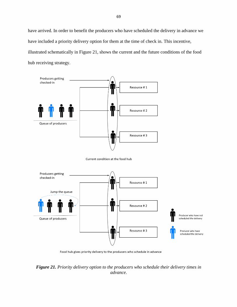
69
have arrived. In order to benefit the producers who have scheduled the delivery in advance we
have included a priority delivery option for them at the time of check in. This incentive,
illustrated schematically in Figure 21, shows the current and the future conditions of the food
hub receiving strategy.
Figure 21. Priority delivery option to the producers who schedule their delivery times in
advance.

70
The surveyed producers were asked about how their decision to schedule their deliveries
to the food hub would change if the food hub provided them with an option of priority delivery.
Figure 22 shows the response of 24 producers in the survey, on how the priority delivery options
affects their scheduling decision with 1 as “not likely” and 5 as “highly likely”.
Figure 22. Survey data showing the effect of priority queue option on the scheduling decision of
the producers.
The decision-making process if the producer is provided with an option of priority
delivery is shown in Figure 23. The corresponding snapshot of the flowchart from the DES
model is shown in Figure 24. A summary of the hybrid ABM-DES model incorporating the
priority delivery option in the producers’ decision-making process is shown in Figure 25.

71
Figure 23. Producer decision-making process with priority delivery option.

72
Figure 24. Snapshot of the Arena simulation model flowchart with priority delivery option.

73
Figure 25. Hybrid simulation (ABM-DES-ABM) model overview with priority delivery option.
Model III - Monetary incentives
Suppliers tend to improve quality if an organization provides incentives to the best
performing suppliers (Modi & Mabert, 2007). Incentives motivate the supplier to implement the
improvements suggested by the buying organization. Firms can motivate suppliers by giving
incentives in the form of sharing the achieved cost saving, recognizing suppliers performance

74
through awards or giving them consideration for increased volumes (Giunipero, 1990; Krause,
Handfield, & Scannell, 1998; Modi & Mabert, 2007). In order to incorporate the possibility of
the food hub’s offering monetary incentives producers who schedule their deliveries, a third
stage was added to the hybrid simulation model, as shown in Figure 26.
Figure 26. Hybrid simulation (ABM-DES-ABM) model overview with food hub agent.
In this version of the hybrid model, a food hub manager agent is included. The food hub
manager calculates the food hub’s revenue in the last n cycles, where n is an experimental value
in the model. Based on the revenue generated, the food hub manager decides to provide
producers a certain percentage of their total sales after the next n cycles as a reward if they
schedule their delivery in advance before arriving at the food hub. The overall decision-making
process of the producer if provided with priority delivery and monetary incentive options is
shown in Figure 27. Figure 28 shows the response of 24 producers on how their decision to
schedule the delivery will affect for the four different monetary incentives level provided by the
food hub with 1 as “not likely” and 5 as “high likely”.

75
Figure 27. Hybrid simulation (ABM-DES-ABM) model overview with monetary incentives and
priority delivery option.

76
Figure 28. Survey data showing the effect of monetary incentives on producers scheduling
decision.
Model IV - Food hub – producer and producer - producer interactions
Suppliers feel motivated to improve if the buying firms communicate with the suppliers
and provide feedback on their performance (Carr & Pearson, 1999). Communication between a
supplier and buying firms can be of two types. First one is the traditional communication e.g.
phone, fax or face-to-face. Second type of communication is advanced communication which
includes computer-to-computer links, enterprise resource planning (ERP) systems or electronic
data interchange (EDI). Since the sophisticated systems required in the advanced communication
methods are not yet well implemented in RFSC, regional food hub managers could implement
traditional communication techniques to communicate with the suppliers to improve their
performance. Also, Leek, Turnbull and Naude (2003) found in their empirical study that
traditional communication is perceived to be more useful by the buying firms as compared to the
advanced communication techniques.

77
Supplier performance could increase if the knowledge transfer occurs between the
network of suppliers. For example, Toyota rewards the supplier who makes an exceptional
knowledge sharing contribution among the network members by giving that supplier additional
business or paying it a bonus for its contributions (Nishiguchi, 1994).
To incorporate the above two conditions in the hybrid simulation model developed, we
have assumed that the food hub manager will communicate with the producers who didn’t
schedule their delivery in an order cycle, and inform them about the inconvenience caused in the
food hub inbound operations due to unscheduled deliveries. In the survey, respondents have been
asked about their satisfaction level while doing business with the food hub. Figure 29 shows the
response of 24 producers in their survey for their satisfaction level of doing business with the
food hub, with 1 as “least satisfied” and 5 as “most satisfied”.
Figure 29. Survey data showing satisfaction level of the survey respondents with respect to
doing business with the food hub.

78
We have used this factor as a probability which will affect producers’ decision to
schedule the delivery in the next cycle if the feedback is given to them by the food hub. It has
been assumed in this model that higher the satisfaction level of the producer with respect to
doing business with the food hub, higher is the probability that the producer will account food
hub feedback in his decision in the next cycle. The probability value has been assigned to 0.8 if
the producer satisfaction level is 5, and is assumed to be linearly decreasing to a value of 0, if the
satisfaction level decreases to 1. Also the producers who change their decision due to this
feedback may convey this information to the other food hub producers thus inspiring them to
schedule the delivery.
In the survey, we have asked how often the producers share their experiences amongst
them they have with the food hub. This is an important parameter in the ABM, as the producers’
decisions can be influenced by information they gain via interactions with other producers
between delivery cycles. For example, they may discuss whether or not they are scheduling their
deliveries and the degree to which scheduling has benefitted them in reducing the queue time at
the food hub. 3 out of 24 producers mention that they don’t interact with the other food hub
producers when they deliver their products at the food hub. Figure 30 show the response of 21
producers, on how often they share their experience while doing business with the food hub with
the other food hub producers. The response was captured on the 5 point Likert scale with 1 as
“never share” and 5 as “always share”.
We have used this response as a probability of interaction between the two producers.
The scale of this probability is defined similarly as described above for the customer satisfaction
level. This interaction among the producers could emerge as all the producers in the system start
scheduling the delivery as they would realize the benefits of it like less waiting time at the food

79
hub altogether. In this model, we have assumed that this producer-producer interaction happens
between a random producer and a producer who gets feedback from the food hub and schedules
the delivery in the next cycle.
Figure 30. Survey data showing how often producers share their business experience with food
hub with the other food hub producers.
The snapshot of NetLogo model (Figure 31) shows the different producer agents for one
order cycle. The agents in “blue” color represent the producers who got feedback from the
producers and decided to schedule the delivery in the next cycle. Agents in “green” color show
the producers who decided to schedule the delivery in the next cycle due to information passed to
them from the “blue” agents.

80
Figure 31. NetLogo model showing food hub – producer and producer-producer interactions.
References
Alexander, M., MacLaren, A., O’Gorman, K., & White, C. (2012). Priority queues: Where social
justice and equity collide. Tourism Management, 33(4), 875-884.
Berger, T., & Schreinemachers, P. (2006). Creating agents and landscapes for multiagent
systems from random samples. Ecology and Society, 11(2), 19.
Brown, D. G., & Robinson, D. T. (2006). Effects of heterogeneity in residential preferences on
an agent-based model of urban sprawl. Ecology and society, 11(1), 46.
Carr, A. S., & Pearson, J. N. (1999). Strategically managed buyer–supplier relationships and
performance outcomes. Journal of operations management, 17(5), 497-519.
Davis, M. M., & Heineke, J. (1998). How disconfirmation, perception and actual waiting times
impact customer satisfaction. International Journal of Service industry Management,
9(1), 64-73.
Giunipero, L. C. (1990). Motivating and monitoring JIT supplier performance. Journal of
Purchasing & Materials Management, 26(3), 19.

81
Grimm, J. (2015, March). Iowa Valley Food Co-op, Cedar Rapids, Iowa. (C. Krejci, Interviewer)
Huber, G. (2015, February). Iowa Food Cooperative, Des Moines, Iowa. (A. Mittal, & C. C.
Krejci, Interviewers)
Krause, D. R., Handfield, R. B., & Scannell, T. V. (1998). An empirical investigation of supplier
development: reactive and strategic processes. Journal of Operations Management,
17(1), 39-58.
Krejci, C. C., & Beamon, B. (2015). Impacts of Farmer Coordination Decisions on Food Supply
Chain Structure. Journal of Artificial Societies and Social Simulation, 18(2), 19.
Krejci, C. C., Stone, R. T., Dorneich, M. C., & Gilbert, S. B. (2015). Analysis of Food Hub
Commerce and Participation Using Agent-Based Modeling Integrating Financial and
Social Drivers. Human Factors: The Journal of the Human Factors and Ergonomics
Society, 1-22.
Leek, S., Turnbull, P. W., & Naude, P. (2003). How is information technology affecting business
relationships? Results from a UK survey. Industrial marketing management, 32(2), 119-
126.
McGuire, K. A., & Kimes, S. E. (2006). The perceived fairness of waitlist-management
techniques for restaurants. Cornell Hotel and Restaurant Administration Quarterly,
47(2), 121-134.
Modi, S. B., & Mabert, V. A. (2007). Supplier development: Improving supplier performance
through knowledge transfer. Journal of operations management, 25(1), 42-64.
Nishiguchi, T. (1994). Strategic industrial sourcing: The Japanese advantage. Oxford University
Press.
Pàmies, M. D., Ryan, G., & Valverde, M. (2015). What is going on when nothing is going on?
Exploring the role of the consumer in shaping waiting situations. International Journal of
Consumer Studies.
Punj, G., & Stewart, D. W. (1983). Cluster analysis in marketing research: review and
suggestions for application. Journal of marketing research, 134-148.
Schreinemachers, P., Berger, T., Sirijinda, A., & Praneetvatakul, S. (2009). The Diffusion of
Greenhouse Agriculture in Northern Thailand: Combining Econometrics and Agent‐Based Modeling. Canadian Journal of Agricultural Economics/Revue canadienne
d'agroeconomie, 57(4), 513-536.
Smajgl, A., Brown, D. G., Valbuena, D., & Huigen, M. G. (2011). Empirical characterisation of
agent behaviours in socio-ecological systems. Environmental Modelling & Software,
26(7), 837-844.

82
Sopha, B. M., Klöckner, C. A., & Hertwich, E. G. (2013). Adoption and diffusion of heating
systems in Norway: coupling agent-based modeling with empirical research.
Environmental Innovation and Societal Transitions, 8, 42-61.
Yim, O., & Ramdeena, K. T. (2015). Hierarchical Cluster Analysis: Comparison of Three
Linkage Measures and Application to Psychological Data. The Quantitative Methods for
Psychology, 11(1), 8-21.

83
CHAPTER 4
SIMULATION RESULTS AND DISCUSSION
There are typically a variety of stakeholders involved with the development and outputs
of a model, including the model developers, decision makers who will use the information from
results of the model to inform their decisions, and individuals affected by these decisions.
Therefore, it is highly important that the model and its results are correct (Sargent, 2005). This
section describes the process of verification and validation for the proposed hybrid simulation
model.
Verification of the hybrid simulation model
Model verification is often defined as “ensuring that the computer program of the
computerized model and its implementation are correct” (Sargent, 2005). The hybrid simulation
model described in this thesis was verified by running the model under specific experimental
conditions and confirming that the input and output variables were consistent with respect to the
specified input conditions and assumptions. We have analyzed the outputs under three different
conditions:
1) Condition 1 – It was assumed in the model that all 72 producer agents will deliver in
every order cycle and producer will deliver in only one of the 11 time slots assigned by
the food hub.
Output verification – The total number of producers delivering to the food hub and the
total number of producers arriving in each of the 11 time slots in every order cycle was
always 72.

84
2) Condition 2 - A producer’s autonomy will be 1 if the producer doesn’t schedule the
delivery. However, if the producer schedules the delivery, the autonomy decreases
linearly from 0.8 to 0 as his satisfaction level for a time slot decreases from 5 to 1.
Output verification - When there is no capacity limit on the time slots in the model, the
autonomy of all the producers was greater than or equal to 0.8 in every order cycle (i.e.,
each producer was able to schedule in his most-preferred time slot).
3) Condition 3 - Time slot capacity was fixed to 6 on distribution day 1 and 18 on
distribution day 2, and every producer was asked to schedule their deliveries as per their
preference level for the time slots
Output verification – In every order cycle, none of the slots has more producers arriving
than the maximum slot capacity
Model I – Status Quo
One strength of empirical simulation models is their ability to be validated with
independent external data. Model validation is usually defined as “substantiation that a
computerized model within its domain of applicability possesses a satisfactory range of accuracy
with the intended application of the model” (Schlesinger, et al., 1979). The initial version of the
hybrid simulation model of the food hub (i.e., Model I) was validated using the historical data
validation technique (Sargent, 2005). This includes comparing outputs of the developed
simulation model with existing historical data of the same system, provided the historical data is
completely independent of the simulation input variables and parameters.
The food hub considered in this study has not placed any capacity restrictions on any of
the 11 time slots for scheduling the delivery (Huber, 2015). Model I represents the same

85
conditions as that of current food hub operations (i.e., the status quo). This version of the model
was run under three different experimental conditions by varying the producers’ weights on
autonomy (WA) and convenience (WC) in the producers’ utility function. As per the survey data,
17 out of 19 producers who correctly answered the ranking question considered flexibility in
schedule (autonomy) as more important than waiting time in queue (convenience) in their
decisions to schedule the delivery. Therefore, in all three experiments, the weight on autonomy
was kept higher than the weight on convenience in an effort to validate the model. For each
experimental scenario, 10 replications of 120 time-steps each were run (where one time step is
equivalent to one “two-week delivery cycle” of the food hub considered in this study). The initial
20 time steps were considered as a warm-up period, to allow the system to stabilize. Therefore,
the final 100 of 120 time-steps were considered for analyzing the simulation results.
Simulation results for the three scenarios with different combinations of weights on
autonomy and convenience are summarized in Table 10. Figure 32 shows the total number of
producers who have decided to schedule their deliveries in each time step over the course of the
simulation run for all the three scenarios. The simulation results show that the average number of
producers scheduling their deliveries increases as the weight on convenience increases. As the
weight on autonomy (WA) was increased from 0.7 to 0.8, there was a large decrease in the
average number of producers scheduling the delivery and reduced variability.

86
Table 10. Summary of number of producers scheduling the delivery for Model I.
Serial
#
Different weight combinations of
autonomy and convenience
Average number of
producers scheduling
the delivery
Standard
deviation
% of total
producers
1
Scenario 1 - (WA) – 0.6, (WC) – 0.4
15.65 0.78 21.74
2
Scenario 2 - (WA) – 0.7, (WC) – 0.3
13.48 0.77 18.73
3 Scenario 3 - (WA) – 0.8, (WC) – 0.2
3.58 0.59 4.97
Figure 32. Number of producers scheduling the delivery in each time step for Scenario 1, 2 and
3 of Model I.
In order to verify that the change in weights significantly affects producers’ behaviors, a
student t-test was performed. Table 11 provides the p-values and the associated conclusions.

87
Table 11. Statistical analysis of the outcomes of three tested scenarios in Model I.
Serial # Comparison t statistic p value Conclusion
1 Scenario 1 vs Scenario 2
-10.84 < 0.00001 H0: μ1 = μ2 is rejected, scenario 1 and
scenario 2 are significantly different from
each other
2 Scenario 1 vs Scenario 3
-38.96 < 0.00001 H0: μ1 = μ2 is rejected, scenario 1 and
scenario 3 are significantly different from
each other
3 Scenario 2 vs Scenario 3
-31.56 < 0.00001 H0: μ1 = μ2 is rejected, scenario 2 and
scenario 3 are significantly different from
each other
Statistical analysis shows that the three scenarios are significantly different from each
other, as the p-values were all nearly zero. Current operations of the food hub considered in this
study have approximately 25% producers scheduling their deliveries in each order cycle. As the
only difference in the input parameters for all the three scenarios is the difference in combination
of weights, and since Scenario 1 yields the simulated percentage of participants that is closest to
the actual system (21.74%), it was concluded that (WA) – 0.6, (WC) – 0.4 represents the most
accurate combination of weights in the producer decision-making process.
Also, in the real food hub system, many producers tend to arrive in the later time slots to
deliver their products (Huber, 2015). Figure 33 shows the simulated number of producers
arriving in each of the 11 time slots for Scenario 1. The simulation results show a pattern that is
similar to the real system, with many producers arriving at the end of the receiving time. Thus
the hybrid simulation model has been validated for two different independent metrics, which
were not used in the development of the model.

88
Figure 33. Number of producers arriving in each time slot for Scenario 1 of Model I.
Figures 34 through 37 summarize the results of running Model I for the critical measures
of system performance: total number of scheduling producers, utilization rate of food hub
personnel, and producer queue time at the food hub. Figure 34 shows number of producers
arriving on delivery days 1 and 2. On average, 40.2 of 72 producers (55.83%) arrive on day 1
and the remaining 31.8 (44.16%) arrive on day 2. On average, 6.8 of the producers arriving on
day 1 (16.9%) are scheduling the delivery and 8.9 of the producers arriving on day 2 (28%) are
scheduling the delivery.

89
Figure 34. Comparison of number of producers arriving and scheduling the delivery on day 1
and day 2 for Scenario 1 of Model I.
Combining multiple deliveries and other activities with the delivery to the food hub was
identified as one of the potential reasons that producers fail to schedule their deliveries. Figure
35 compares the average number of producers not scheduling their deliveries per order cycle due
to combining multiple deliveries in the area and harvesting schedule. On average, 34.4 of the 72
producers (47.7%) do not schedule their deliveries in an order cycle due to multiple deliveries
and other activities in the area and 15.2 (21.1%) due to their harvesting schedule uncertainty.
Figure 36 shows the average man hour utilization rate on day 1 and day 2, calculated
using the following expression:
𝑀𝑎𝑛 ℎ𝑜𝑢𝑟 𝑢𝑡𝑖𝑙𝑖𝑧𝑎𝑡𝑖𝑜𝑛 𝑟𝑎𝑡𝑒 = ( 𝑇𝑜𝑡𝑎𝑙 𝑚𝑎𝑛 ℎ𝑜𝑢𝑟𝑠 𝑠𝑝𝑒𝑛𝑡 𝑜𝑛 𝑟𝑒𝑐𝑒𝑖𝑣𝑖𝑛𝑔 𝑝𝑟𝑜𝑐𝑒𝑠𝑠
𝑇𝑜𝑡𝑎𝑙 𝑎𝑣𝑎𝑖𝑙𝑎𝑏𝑙𝑒 𝑚𝑎𝑛 ℎ𝑜𝑢𝑟𝑠 )
A total of 2 volunteers are available for 8 hours on receiving day 1 (i.e., 16 man hours) and 6
volunteers are available for 3 hours on day 2 (i.e., 18 man hours). As Figure 34 shows, fewer
producers arrive on day 2 (44.16%) and there are more man hours available, resulting in a lower

90
average utilization on day 2 (0.5) than on day 1 (0.7). However, this represents the utilization
rates as averages over each day. As Figure 33 shows, very few producers arrive in the 1st, 3rd and
5th slot on day 1; therefore, the utilization rate for these specific time slots will be significantly
less than the average. Also, on delivery day 2, the utilization rate in slot 11 on day 2 will be
higher than the average rate 0.5.
Figure 35. Average number of producers not scheduling their deliveries due to multiple
deliveries and harvesting schedule for Scenario 1 of Model 1.
Figure 37 shows the average queue times of the producers on day 1 and day 2. The longer
average queue time on day 1 is a result of variability in producer arrival times (especially a
greater number of producers arriving in the 2nd and 6th slots of day 1), with only 2 volunteers
available for the receiving process. This is because the food hub manager has not placed any
capacity limits on the time slots. As such, many producers arrive at the same time slot (as per
their preferences), whether they scheduled their deliveries or not.

91
Figure 36. Average man hour utilization rate on day 1 and day 2 for Scenario 1 of Model I.
Figure 37. Average queue time on day 1 and day 2 for Scenario 1 of Model I.

92
Originally, it was expected that the average queue time would decrease as more
producers decided to schedule their deliveries. In order to test this, the average queue time for the
three different scenarios of Model I were compared. The results exhibit variability in the number
of producers scheduling their deliveries as the weights on autonomy and convenience (WA and
WC, respectively) were changed. Figures 38 and 39 show the average queue times on day 1 and
day 2 versus the number of producers scheduling their deliveries on the respective days in the
three scenarios. Interestingly, the average queue times on day 1 very slightly increased from
Scenario 1 to Scenario 2 and from Scenario 2 to Scenario 3. The average queue time on day 2
increases from Scenario 1 to Scenario 2 and decreases from Scenarios 2 and 3. The statistical
analysis shows that the average queue time for day 1 and day 2 is similar for all the three
scenarios with α = 0.05. This outcome makes intuitive sense - as there is no capacity limit on the
time slots, the number of producers arriving in each time slot depends only on their preferences
for the time slots, regardless of whether they are scheduling the delivery or not. This is because,
if a producer decides not to schedule, he will arrive in one of his most preferred time slot and if a
producer decides to schedule the delivery, as there is no capacity restrictions on the time slots, he
get to schedule and arrive in his most preferred time slot. This leads to nearly the same number
of producers arriving in each time slot for all the three scenarios irrespective of number of
producers scheduling the deliveries and hence the average queue time within the scenarios
doesn’t differ significantly.

93
Figure 38. Average queue time vs number of producers scheduling the delivery on day 1 for
Scenarios 1, 2, and 3 of Model I.
Figure 39. Average queue time vs number of producers scheduling the delivery on day 2 for
Scenarios 1, 2, and 3 of Model I.

94
Food Hub Interventions
This section describes the effects of various policies that the food hub can adopt to
encourage producers to schedule their deliveries. The Scenario 1 weights (WA= 0.6, WC = 0.4)
were used because they are assumed to represent the most accurate combination of weights in the
producers’ decision-making process.
Model II – Priority delivery option by the food hub
When the food hub provided an incentive of priority delivery to the producers who
scheduled their deliveries, an average of only 12.33 producers (17.13%) scheduled the delivery.
This outcome shows that the priority delivery option can actually demotivate the producers who
were already scheduling. Figure 40 shows the number of producers scheduling the delivery and
the ones who are actually benefiting from the priority delivery incentive in each time step. As
described in Chapter 3, a producer will be consider benefitted from the priority delivery option,
if his waiting time in the queue at the food hub even after getting priority delivery, falls in the
time range of his maximum satisfaction level. This satisfaction level for the wait time ranges
have been identified from the producers’ survey data. In 20% of the order cycles even if a
producer schedules the delivery, he is not able to benefit from the priority delivery incentive
provided by the food hub (Figure 41). This is because even if the producer is allowed to jump to
the front of the queue, he may still have to wait until at least one of the volunteers is available for
the receiving process. If this wait time does not yield a satisfactory utility level, the producer will
not schedule his delivery in the next cycle, as he did not experience any benefits from
scheduling. Figure 42 shows the number of producers in each time step who scheduled the
delivery specifically because of the benefit resulting from the priority delivery incentive in the

95
previous cycle. On average, only 2.2 producers (3.3%) were motivated by this incentive to
schedule their delivery in the next cycle.
Figure 40. Number of producers scheduling and benefiting from the priority delivery incentive in
each time step of Model II.
Figure 41. Average overall number of producers scheduling and benefiting from the priority
delivery incentive in Model II.

96
Figure 42. Number of producers scheduling in each time step in Model II due to benefits of
priority delivery in the previous cycle.
Recommendation to the food hub - The priority delivery option will likely only benefit
the food hub under certain conditions:
1) The food hub should place a capacity limit on the number of producers who are allowed
to schedule their deliveries in each time slot .Otherwise, having more producers schedule
their deliveries will not necessarily lead to a more balanced workload at the food hub,
because there are certain time slots which many producers tend to prefer (e.g., the last
time slot in day 2). This will cause dissatisfaction and possibly resentment among the
producers who, even after scheduling the delivery, must wait in long queues to get their
products checked in.
2) To benefit the entire system, enough producers must schedule their deliveries to outweigh
the costs of the “freeloaders” who do not schedule. If the food hub merely puts capacity
limits on the time slots, there will be many producers who will arrive at the same time
slots whether they schedule or not, and it will create disillusionment among the producers

97
who scheduled their deliveries but had to wait in the queue for a long time anyway. To
demonstrate the effects of placing a capacity limit on the time slots when there is a
priority queue incentive, the average number of producers who schedule was captured for
a modified version of Model II. Given that the average time for a food hub volunteer to
check in a producer is 16.8 minutes, to have the shortest possible queue times, each
volunteer should check in three producers per hour. Therefore, on day 1, a capacity limit
of 6 was assigned to all 8 time slots, and on day 2, a capacity limit of 18 was assigned to
all three time slots. Figure 43 shows that the average number of producers scheduling the
delivery is almost the same as that of previous case when there were no limits on the time
slots, with an average of 12.4 producers (17.2%) scheduling. A t-test comparing the two
averages gives a p-value of 0.55, which clearly shows that the scenarios are not
significantly different from one another, indicating that putting limits on the time slot
capacities does not affect the producers’ decisions.
Figure 43. Average number of producers scheduling and benefiting from the priority delivery
incentive if the food hub puts capacity limit on the time slots in Model II.
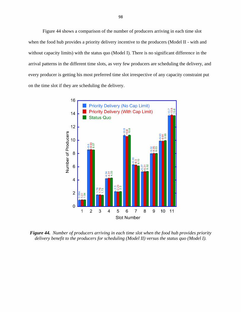
98
Figure 44 shows a comparison of the number of producers arriving in each time slot
when the food hub provides a priority delivery incentive to the producers (Model II - with and
without capacity limits) with the status quo (Model I). There is no significant difference in the
arrival patterns in the different time slots, as very few producers are scheduling the delivery, and
every producer is getting his most preferred time slot irrespective of any capacity constraint put
on the time slot if they are scheduling the delivery.
Figure 44. Number of producers arriving in each time slot when the food hub provides priority
delivery benefit to the producers for scheduling (Model II) versus the status quo (Model I).

99
Model III – Monetary and priority delivery incentives
When the food hub offers a monetary incentive along with the priority delivery incentive
to those producers who schedule their deliveries, on average 42 producers (58.3%) schedule, at
an average incentive level of 3.79% of total producer sales. This incentive level is calculated by
taking the mean of the monetary incentives range as asked in the survey. For example, if the food
hub decides to provide between 1 to 3 % of total sales of a producer as a monetary incentive to
the producers for scheduling the delivery, it has been considered that the mean of this incentive
range is provided by the food hub in all the iterations of the Model III. Also it has been
considered that a maximum of 6% of total sales of a producer is provided by the food hub as a
monetary incentive to the producers for scheduling the delivery. However, a food hub would
need to carefully assess the tradeoff between the cost of providing the incentive and the
operational benefits of having more producers schedule their deliveries.
In this model it has been assumed that the food hub has imposed a capacity limit on the
time slots. On day 1, a capacity limit of 6 was assigned to all 8 time slots, and on day 2, a
capacity limit of 18 was assigned to all three time slots. Figure 45 shows the number of
producers scheduling in each time step and the monetary incentive level provided by the food
hub in corresponding time steps. The R-square value when linearly fitting the monetary incentive
percentage values versus number of producers scheduling the delivery is 0.75, which indicates a
linear relationship between the two. A t test was performed to test the null hypothesis (H0: β1 =
0). The p-value of the t test was < 0.0001, confirming this linear relationship. Figure 46 shows
the average queue times on day 1 and day 2. There is 21.12 % decrease in average queue time on
day 1 from the current conditions at the food hub (i.e., Model I), and on day 2 the average queue
time is almost the same.

100
Figure 45. Number of producers scheduling the delivery and percentage monetary incentive of
a producer total sales provided by the food hub in each time step of Model III.
Figure 46. Average queue time on day 1 and day 2 if the food hub provides monetary incentive
benefits to the scheduling producers in Model III.

101
Recommendation to the food hub – Even though the number of producers scheduling the
delivery increases by 168.37% as compared to the current food hub operating conditions, the
average queue time on day 1 decreases only by 21.12%. The potential reason for this is that
many producers prefer particular time slots, while in some slots very few producers show up.
Figure 47 compares the number of producers arriving in each time slot for Models I and III.
Though more producers schedule their deliveries and the food hub has put capacity limits on the
time slots, these limits are often exceeded because of the arrival of unscheduled producers. The
2nd and 6th slots have the maximum number of producers arriving on day 1. The average queue
time has not decreased significantly as the number of producers arriving in those two time slots
has not decreased significantly. The average queue time on day 1 is high due to around 8.6
producers arriving in the 2nd slot and 10.8 producers in the 6th slot for the status quo conditions.
However, when more producers are scheduling due to monetary and priority queue incentives,
the number of producers scheduling in this time slot doesn’t decrease significantly. This may
also lead to fewer producers scheduling their deliveries due to long wait times, despite
scheduling in advance. Therefore, in addition to providing monetary incentives, the food hub
should also re-allocate its volunteer labor to have more volunteers working during the the most-
preferred time slots of the producers.
As mentioned in the results of Model II, the priority delivery incentive will be useful for
the food hub to implement if capacity limits are placed on the time slots and if enough producers
schedule their deliveries that the overall system benefits. This recommendation is explained with
the outcomes of Model III. Figure 48 shows the comparison of number of producers who are
unaffected by the monetary incentives but schedule their deliveries due to the benefits of priority
delivery in the previous cycle in Model III and the number of producers who are scheduling their

102
delivery due to priority delivery benefits in previous cycle in Model II (without capacity limits
on time slots). In Model III capacity limits were placed by the food hub on the time slots and also
58.3% of the producers were scheduling the delivery on average in an order cycle. The average
number of producers scheduling the delivery got increased as compared to Model II due to the
monetary incentives provided by the food hub. This resulted the system with more uniform
arrival time of producers in the 11 time slots, which leads to greater benefits to the producers
who are scheduling the delivery due to priority delivery incentive. In Model III an average of 6.8
producers (9.4%) scheduling their deliveries due to only priority delivery benefits, which three
times larger than the number of producers who scheduled when there were no capacity limits and
only around 12.3% of the producers scheduled their deliveries in Model II.
Figure 47. Number of producers arriving in each time slot when the food hub provides
monetary incentives to the producers for scheduling (Model III) versus the status quo (Model I).

103
Figure 48. Comparison of number of producers who are not affected by monetary incentives
provided by the food hub but schedule due to benefits of priority delivery in the previous cycle in
Model III vs number of producers who schedule the delivery due to priority delivery option in
Model II (without capacity limit on time slots).
Model IV – Agent interactions
Figure 49 shows the number of producers scheduling their deliveries in each time step for
Model IV, when the food hub provides feedback to the producers with respect to scheduling their
deliveries. On average, 40 producers (55.85%) schedule their deliveries in each cycle. In this
model, the probability that an interaction between two producers will lead to scheduling is
assumed to be 50%.
Figure 50 shows the number of producers scheduling the delivery due to feedback from
the food hub to the producers and due to successful interactions among the food hub producers in
each time step for Model IV. Due to food hub–producer interactions, on average 19.8 producers
(27.57%) schedule their deliveries in the next cycle (Figure 51). The average percentage of

104
successful interactions between the food hub and a producer is 61.92%, which is the ratio of the
number of producers to which the food hub gives the feedback to the number of producers who
become motivated to schedule the delivery in next cycle based on the feedback. Also, on
average, 2.9 producers (4%) schedule their deliveries upon becoming motivated by other food
hub producers. On average, 14.9 % of the time a producer is able to motivate another producer to
schedule the delivery in the next cycle.
Figure 49. Number of producers scheduling the delivery in each time step when the food hub
provides feedback to the producers and producers interact with each other to share information
in Model IV.
Recommendation to the food hub – It is evident from Figures 47 and 52 that even if more
producers schedule their deliveries (58.3% and 55.85%), 2nd and 6th time slots are having more
number of producers coming, due to the individual preferences of the producers who schedule or
doesn’t schedule the delivery. Also in 1st, 3rd and 5th time slot, very few producers show up.
Therefore the food hub should consider re-allocation of their volunteer labor in order to reduce
producer queue time and efficiently utilize their resources.

105
Figure 50. Number of successful food hub-producer and producer-producer interactions in
Model IV.
Figure 51. Number of successful interactions between the food hub and a producer and between
two producers in Model IV.

106
Figure 52. Number of producers arriving in each time slot when food hub provide provides
feedback to the producers for scheduling (Model IV) versus the status quo (Model I).
References
Huber, G. (2015, February). Iowa Food Cooperative, Des Moines, Iowa. (A. Mittal, & C. Krejci,
Interviewers)
Sargent, R. G. (2005). Verification and Validation of Simulation Models. Proceedings of 2005
Winter Simulation Conference (pp. 30-143). IEEE.
Schlesinger, S., Crosbie, R. E., Gagné, R. E., Innis, G. S., Lalwani, C. S., Loch, J., . . . Bartos, D.
(1979). Terminology for model credibility. Simulation, 32(3), 103-104.
107
CHAPTER 5
CONCLUSION
General Conclusions
Producer delivery scheduling has the potential to improve a regional food hub’s inbound
operations by helping it to appropriately allocate its resources and provide better service to its
customers through better product quality and fewer order errors. This will likely increase
customer loyalty and business for the food hub, thereby improving the economic growth
opportunities and quality of life for participating small and mid-sized producers. However,
encouraging producers to schedule their deliveries can be very challenging for a food hub
manager. Producers greatly value their autonomy, and they tend to resist having constraints
placed on their ability to set their own schedules, although some producers may be willing to
give up some autonomy in exchange for greater convenience or a financial incentive. Producers’
delivery scheduling decisions may also be influenced by social interactions that they have with
one another, in which they share information about their experiences with scheduling. As a
result, predicting the effects of specific management policies on producer scheduling behavior
and subsequent system-wide outcomes is very difficult
To address this problem, an empirical hybrid simulation model of the inbound logistics
operations at a regional food hub in Iowa was developed. The model was used to study the
impacts of producers’ delivery scheduling behavior on food hub warehouse operations and to
analyze the feasibility and outcomes of implementing various corrective actions. Discrete event
simulation was used to represent the arrivals and queueing behavior of producers at the
warehouse, and agent-based modeling was used to represent producer decision making and

108
interactions. This hybrid model was informed by empirically-derived human and system data,
which reflected the actual heterogeneous decision-making processes and behaviors of the food
hub’s participants.
Four versions of the model were described in this thesis. In Model I, the current operating
conditions at the food hub were captured. This model was validated using the food hub’s
historical data, which is independent of the input data that was used to construct the model.
Models II, III, and IV were used to observe the effects of different food hub policies on
producers’ scheduling behavior. Experimental results from Model II suggest that, if implemented
inappropriately, incentives can be counterproductive. The results also indicate that increased
producer scheduling by itself does not necessarily improve system outcomes. Although advance
scheduling provides useful information to the food hub manager, if he does not act on this
information (e.g., by scheduling more receiving personnel to work during the producers’ most-
preferred time slots), neither the food hub nor the producers will benefit.
This thesis demonstrates the need for a hybrid modeling methodology to realistically
represent complex sociotechnical behaviors in regional food supply chains. Because agent
interactions were not included in Models I and II, it may have been possible to develop these
versions of the model using DES alone. However, using DES to model the interactions between
the food hub and producers and among the producers in Models III and IV would have
impractical. Also, modeling the process-oriented framework (e.g., the priority delivery queuing
behavior in Model II) would have been extremely difficult to model and validate using ABM.

109
Limitations and Future Work
The outcomes of this research can help food hub managers to frame policies that will
improve the effectiveness and efficiency of their inbound operations. In future research, it would
be interesting to observe how the agents belonging to different behavioral clusters respond to
different food hub policy implementations. This will help the food hub manager determine how
best to structure incentives to obtain optimal results. For example, producers in Cluster 1 are
highly influenced by monetary incentives. However, the results show that even when monetary
incentives are offered by the food hub, producers arrival times are concentrated in particular time
slots due to the producers who refuse to schedule their deliveries. Therefore, the food hub might
consider modifying the monetary incentive by informing the producers that they will receive the
benefit only if they arrive in the less desirable time slots. It would be interesting to observe how
the behavioral patterns of the producers who were scheduling regularly because of the monetary
incentive might change with the implementation of a modified policy.
Additionally, incorporating greater heterogeneity among agents in the system may enable
a more realistic representation of the system. In the model presented in this thesis, the utility
functions for each producer agent were assumed to be identical. In a future version of the model,
heterogeneous utility functions based on individual preferences for autonomy and convenience
will be included, based on survey data. Other producer-specific factors could also be
incorporated. For example, product type may influence the decision to schedule – requirements
for scheduling flexibility can greatly vary for shelf-stable, frozen, and refrigerated goods. The
distance that a producer must travel to deliver goods to the food hub warehouse may also impact
scheduling decisions.

110
Another possible future development of the model presented in this thesis is the inclusion
of multiple Iowa food hubs, enabling the collection of information from a wider variety of
producers and food hub managers. This would improve the generalizability of the model and
would allow implications from experimental results to be extended to other food hubs, thereby
increasing the model’s usefulness as a decision support tool for food hub managers.
Model IV was developed to demonstrate the usefulness of ABM in modeling food hub
operations. Future work will include producers’ interactions based on their arrival patterns at the
food hub. Such interactions could occur between the producers who are waiting in the queue at
the food hub, leading to shared knowledge and experiences. The impact of these social
interactions on producers’ behaviors toward the food hub would be interesting to explore using
ABM.
The possibility of using simulation software that has both ABM and DES capabilities
(i.e., AnyLogic), or using distributed simulation techniques to automate the integration of two
different simulation platforms is currently being explored. This will potentially speed up the
execution of the simulation runs, making experimentation more efficient.
Regional food hubs provide a potential solution to the problem of unmet and growing
demand for regionally and sustainably-produced food in the United States. However, financial
constraints and a strong social mission often prevent them from employing conventional supply
chain practices in their operations. Helping food hub managers to address the complex challenge
of balancing operational efficiency and social responsibility is critical to food hub success, which
has implications for the long-term viability of regional food systems and their participants.

111
APPENDIX A
PRODUCER SURVEY QUESTIONNAIRE
The purpose of this survey is to gather information on the factors that influence your decision
to schedule the delivery at the food hub.
The data collected in this survey will be used to help the food hub managers to take strategic
decisions in order to improve their warehouse operations efficiency.
Your answers to the survey questions will be kept confidential.
Please feel free to contact Dr. Caroline C. Krejci at Iowa State University, if you have any
questions or concerns at [email protected].
Thank you in advance for your contribution in conducting this research study!
Questions for food hub producers.
General information
1) What is your producer ID?
2) How satisfied are you with your business with the food hub?
a. Extremely satisfied
b. Very satisfied
c. Moderately satisfied
d. Not very satisfied
e. Not at all satisfied
3) How far do you live from the food hub?
a. < 5 miles
b. >=5 miles and < 15 miles
c. >= 15 miles and < 30 miles
d. >= 30 miles and < 45 miles
e. >= 45 miles

112
Scheduling behavior
4) How do you deliver your products to the food hub?
a. Ship the products
b. Deliver yourself
c. Someone else deliver on your behalf
d. Other________________________________________________________
5) Are you aware that the food hub gives an option to schedule your delivery online?
a. Yes
b. No
6) How often do you schedule the delivery online before arriving to the food hub?
a. Every cycle
b. Every alternate cycle
c. Once in 2 months
d. Once in 3 months
e. Once in 6 months
f. Never
7) On the scale of 1 to 5 (“1” as least preferred, “5” as most preferred), what is your preference for
delivery in each of the following time slots?
a. Day before delivery day (Wednesday)
I. 9:00 – 10:00 a.m. Least preferred ---1---2—3—4—5---Most preferred
II. 10:00 – 11:00 a.m. Least preferred ---1---2—3—4—5---Most preferred
III. 11:00 – 12:00 p.m. Least preferred ---1---2—3—4—5---Most preferred
IV. 12:00 – 1:00 p.m. Least preferred ---1---2—3—4—5---Most preferred
V. 1:00 – 2:00 p.m. Least preferred ---1---2—3—4—5---Most preferred
VI. 2:00 – 3:00 p.m. Least preferred ---1---2—3—4—5---Most preferred
VII. 3:00 – 4:00 p.m. Least preferred ---1---2—3—4—5---Most preferred
VIII. 4:00 – 5:00 p.m. Least preferred ---1---2—3—4—5---Most preferred

113
b. On delivery day (Thursday)
IX. 9:00 – 10:00 a.m. Least preferred ---1---2—3—4—5---Most preferred
X. 10:00 – 11:00 a.m. Least preferred ---1---2—3—4—5---Most preferred
XI. 11:00 – 12:00 p.m. Least preferred ---1---2—3—4—5---Most preferred
8) If your most preferred time slot(s) is/are not available, would you still schedule the delivery in a less
preferred available slot?
a. Yes
b. No
9) On the scale of 1 to 5 (“1” is least satisfied and “5” as most satisfied) what will be your satisfaction
level for the following waiting times to have your products inspected and checked in by the IFC
volunteers?
a. < 5 minutes Least satisfied---1---2—3—4—5---Most satisfied
b. >=5 and < 10 minutes Least satisfied---1---2—3—4—5---Most satisfied
c. >=10 and <15 minutes Least satisfied---1---2—3—4—5---Most satisfied
d. >=15 minutes and <20 minutes Least satisfied---1---2—3—4—5---Most satisfied
e. >= 20 minutes and <25 minutes Least satisfied---1---2—3—4—5---Most satisfied
f. >= 25 minutes and < 30 minutes Least satisfied---1---2—3—4—5---Most satisfied
g. > 30 minutes Least satisfied---1---2—3—4—5---Most satisfied
10) Are you the producer of the items that you are delivering?
a. Yes
b. No
11) Do you typically incorporate your delivery with other activities in the area?
a. Yes
b. No

114
11.a. If YES, what activities?
a. For full time employment
b. For other deliveries
c. For personal activities
d. Other: _________________________________________________
11.b. If YES, how likely is it that this affects your decision to schedule the delivery?
Not likely---1---2—3—4—5---Highly likely
12) How good is the internet connectivity at your residence/ workplace?
Low---1---2—3—4—5---High
13) How often do you combine/ coordinate the deliveries to the food hub with other producers?
a. Every cycle
b. Every alternate cycle
c. Once in 2 months
d. Once in 3 months
e. Once in 6 months
f. Never
13.a. If the food hub offers you monetary incentives to coordinate/share the delivery, how likely
would you be to coordinate your delivery with other producers?
Not likely---1---2—3—4—5---Highly likely
14) How will your decision to schedule the delivery change for each of the following monetary incentive
levels provided by the food hub?
a. <1% of your total sales (in one cycle) No effect---1---2—3—4—5---Always schedule
b. >=1 and < 3% of your total sales No effect---1---2—3—4—5---Always schedule
c. >=3 and <5% of your total sales No effect---1---2—3—4—5---Always schedule
d. >=5 % of your total sales No effect---1---2—3—4—5---Always schedule

115
15) If the food hub offers you priority delivery (i.e. go to the front of the line for receiving) as an
incentive to schedule, how likely would you be to schedule your delivery?
Not likely---1---2—3—4—5---Highly likely
16) Do you interact with other food hub producers?
a. Yes
b. No
16. a. If YES, how many producers on average do you interact within an order cycle?
c. 1
d. 2
e. 3
f. 4
g. 5 or more
16.b. If you interact with other producers, how often do you share the experiences you have with
the food hub?
Never---1---2—3—4—5---Always
17) Do you harvest, pack and label the products on the day of delivery?
a. Yes
b. No
17.a. If YES, how likely is it that this affects your decision to schedule the delivery?
Not likely---1---2—3—4—5---Highly likely
18) With “1” as most influential and “8” as least influential, rank the following factors according to how
strongly they affect your decision to schedule the delivery:
a. Convenience of internet access ___
b. Flexibility in delivery ___
c. Wait time for product inspection/check in by volunteers ___
d. Combine/coordinating delivery with other producers ___

116
e. Combining your delivery with other activities near the food hub ___
f. Monetary incentives from the food hub ___
g. Priority delivery incentive from the food hub ___
h. Harvesting and packing schedule ___
19) Are there any other factors that influence your decision to schedule your delivery at the food hub?
Factor 1: __________________________________________________________________
Factor 2: __________________________________________________________________
Factor 3: ___________________________________________________________________
Factor 4: ___________________________________________________________________
19.a. If there are any other factors, where within the 8 factors mentioned above (question #20)
would you rank these factors?
Factor 1 between _____and _____ (mention the ranks associated with the factors)
Factor 2 between _____and _____
Factor 3 between _____and _____
Factor 4 between _____and _____

117
APPENDIX B
AGGLOMERATIVE SCHEDULE
Recommended