Received: 23 October 2016 Accepted: 25 September 2017
DO
I: 10.1002/hyp.11371R E S E A R CH AR T I C L E
Hurricanes and tropical storms: A necessary evil to ensurewater supply?
Meijing Zhang1,2 | Xing Chen1 | Mukesh Kumar1 | Marco Marani1 | Michael Goralczyk1
1Nicholas School of the Environment, Duke
University, Durham, NC 27708, USA
2Department of Agricultural and Biological
Engineering, University of Florida, Homestead,
FL 33031, USA
Correspondence
Mukesh Kumar, Nicholas School of the
Environment, Duke University, Durham, NC
27708, USA.
Email: [email protected]
Funding information
Hunt Oil Company; National Science Founda-
tion, Grant/Award Numbers: EAR‐1331846and EAR‐1454983
Hydrological Processes. 2017;1–15.
AbstractSeveral parts of the globe including Southeast North America, the Caribbean, Southeast Asia,
Australia, and China are often hit by hurricanes and tropical storms (HTSs), which can deliver a
large amount of rainfall within a period of a few days. Although HTSs are mostly studied as
disaster agents, considering that they occur during the period when water supply systems are
generally depleted, it is important to ascertain their potential contributions toward sustaining
water supply. Using the Lake Michie–Little River reservoir system that supplies water to the city
of Durham (North Carolina) as a representative test case, we implemented an integrated water-
shed and reservoir management model, supported by publicly available observations, to evaluate
the extent to which HTSs impact water storages. Results indicate that HTSs can have a significant
impact on reservoir water storage, with their effects being felt for more than a year for some
storms. The impact on reservoir water storage is identified to be primarily controlled by 3 factors,
namely, streamflow response size from HTSs, storage in the reservoir right before the event, and
streamflow succeeding the event response to HTS (henceforth referred as postevent
streamflow). Although the impact of streamflow response size on water storage is generally
proportional to its magnitude, initial water storage in the reservoir and postevent streamflow
have a nonmonotonic influence on water storage. As all the 3 identified controls are a function
of antecedent hydrologic conditions and meteorological forcings, these 2 factors indirectly influ-
ence the impact of HTS on water storage in a reservoir. The identification of controlling factors
and assessment of their influence on reservoir response will further facilitate implementation of
more accurate estimation and prediction frameworks for within‐year reservoir operations.
KEYWORDS
distributed hydrologic modelling, drought, hurricanes, reservoir management, tropical storms, water
supply
1 | INTRODUCTION
It is estimated that on Earth there are more than 16.7 million reservoirs
with a surface area larger than 1 × 10⁻⁴ km2 (Lehner et al., 2011).
These reservoirs provide numerous functions, including municipal
water supply, irrigation, flood control, hydro‐power production, and
navigation. Functional efficiency and resiliency of reservoirs, especially
the water‐supply reservoirs, is crucially dependent on their storage
capacity. Larger reservoirs, with volumes much greater than the mean
annual cumulative flow, function as “over‐year systems”; that is, they
are operated according to multiyear regulation schemes (Anderson
et al., 2008; Carpenter & Georgakakos, 2001; Graf, 1999; McMahon,
wileyonlinelibrary.com/journa
Pegram, Vogel, & Peel, 2007; Vogel & Bolognese, 1995; Yao &
Georgakakos, 2001). These reservoirs are typical of semiarid regions
such as the Southwestern United States and are built to be resilient
to seasonal to interannual inflow variability (Graf, 1999; McMahon
et al., 2007). In contrast, smaller storage capacity reservoirs generally
act as “within‐year systems” with discharge and storage rules designed
to sustain water demands for a year (Graf, 1999; McMahon et al.,
2007). Because of their smaller size, these reservoirs may be vulnera-
ble to seasonal, monthly, and even daily variations in hydrologic
inflows and water demands (Hanak & Lund, 2012; Pagano & Garen,
2005; Vogel & Bolognese, 1995; Weaver, 2005). As coastal regions
of North and Central America, the Indian subcontinent, Southeast Asia
Copyright © 2017 John Wiley & Sons, Ltd.l/hyp 1
2 ZHANG ET AL.
and Africa, Indo‐Malaysia, and Northern Australia are often hit by
hurricanes and tropical storms (HTSs; Gray, 1975; Lott & Ross, 2006;
Michener, Blood, Bildstein, Brinson, & Gardner, 1997; Powell & Keim,
2015), which can deliver a large amount of rainfall within a period of
a few days, a natural question is whether these storms play a signifi-
cant role in determining within‐year reservoir water storage.
Although HTSs have been mostly analysed in terms of their disas-
trous implications (Ashley & Ashley, 2008; Changnon, 2009; Dale et al.,
2001; Elsner, 2007; Emanuel, 1987; Emanuel, Sundararajan, &
Williams, 2008; Saunders, Chandler, Merchant, & Roberts, 2000),
this study explores their potential positive role in generating
water supply. We hypothesize that, especially during times
of drought (Chowdhury, 2010; Chu et al., 2002; Golembesky,
Sankarasubramanian, & Devineni, 2009; Merabtene, Kawamura, Jinno,
& Olsson, 2002; Nakagawa et al., 2000; Wilhite, 1997; Wilhite &
Svoboda, 2000), when depleted local water storages have been known
to cause severe hardships in municipalities, rain delivered by HTSs may
provide a crucial contribution to water supply. Our research goals are
to (a) evaluate the extent to which HTSs may impact reservoir water
storage, especially in drought years when supply is more vulnerable,
and (b) identify the hydrologic controls on HTSs' impact on reservoir
storage and assess their individual influences.
2 | DATA AND METHODS
2.1 | Study area and datasets
We use a reservoir system in Southeastern United States, which is
often hit by HTSs and droughts (Carter, 1999; White & Wang, 2003),
as a representative test case for analyses. One other reason for the
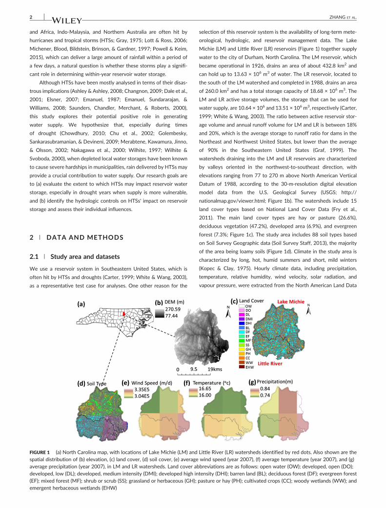
FIGURE 1 (a) North Carolina map, with locations of Lake Michie (LM) andspatial distribution of (b) elevation, (c) land cover, (d) soil cover, (e) averageaverage precipitation (year 2007), in LM and LR watersheds. Land cover abdeveloped, low (DL); developed, medium intensity (DMI); developed high in(EF); mixed forest (MF); shrub or scrub (SS); grassland or herbaceous (GH);emergent herbaceous wetlands (EHW)
selection of this reservoir system is the availability of long‐term mete-
orological, hydrologic, and reservoir management data. The Lake
Michie (LM) and Little River (LR) reservoirs (Figure 1) together supply
water to the city of Durham, North Carolina. The LM reservoir, which
became operational in 1926, drains an area of about 432.8 km2 and
can hold up to 13.63 × 10⁶ m3 of water. The LR reservoir, located to
the south of the LM watershed and completed in 1988, drains an area
of 260.0 km2 and has a total storage capacity of 18.68 × 10⁶ m3. The
LM and LR active storage volumes, the storage that can be used for
water supply, are 10.64 × 10⁶ and 13.51 × 10⁶ m3, respectively (Carter,
1999; White & Wang, 2003). The ratio between active reservoir stor-
age volume and annual runoff volume for LM and LR is between 18%
and 20%, which is the average storage to runoff ratio for dams in the
Northeast and Northwest United States, but lower than the average
of 90% in the Southeastern United States (Graf, 1999). The
watersheds draining into the LM and LR reservoirs are characterized
by valleys oriented in the northwest‐to‐southeast direction, with
elevations ranging from 77 to 270 m above North American Vertical
Datum of 1988, according to the 30‐m‐resolution digital elevation
model data from the U.S. Geological Survey (USGS; http://
nationalmap.gov/viewer.html; Figure 1b). The watersheds include 15
land cover types based on National Land Cover Data (Fry et al.,
2011). The main land cover types are hay or pasture (26.6%),
deciduous vegetation (47.2%), developed area (6.9%), and evergreen
forest (7.3%; Figure 1c). The study area includes 88 soil types based
on Soil Survey Geographic data (Soil Survey Staff, 2013), the majority
of the area being loamy soils (Figure 1d). Climate in the study area is
characterized by long, hot, humid summers and short, mild winters
(Kopec & Clay, 1975). Hourly climate data, including precipitation,
temperature, relative humidity, wind velocity, solar radiation, and
vapour pressure, were extracted from the North American Land Data
Little River (LR) watersheds identified by red dots. Also shown are thewind speed (year 2007), (f) average temperature (year 2007), and (g)breviations are as follows: open water (OW); developed, open (DO);tensity (DHI); barren land (BL); deciduous forest (DF); evergreen forestpasture or hay (PH); cultivated crops (CC); woody wetlands (WW); and
ZHANG ET AL. 3
Assimilation System phase 2 (NLDAS‐2) meteorological forcing dataset
(Xia et al., 2012). These forcing data have a spatial resolution of about
9.5 km in the study area (Mitchell et al., 2004; Figure 1e–g).
2.2 | Distributed hydrologic model implementation
The Penn State Integrated Hydrologic Model (PIHM; Kumar, 2009; Qu
& Duffy, 2007) was applied to both the LM and LR watersheds to simu-
late streamflow into the two reservoirs and to evaluate the impact of
individual HTSs on water storage in the reservoirs. The model has been
previously applied at multiple scales and in diverse hydro‐climatological
settings for simulating streamflow and coupled hydrologic process
dynamics (Chen, Kumar, & McGlynn, 2015; Kumar & Duffy, 2015;
Kumar, Marks, Dozier, Reba, & Winstral, 2013; Liu & Kumar, 2016;
Seo, Sinha, Mahinthakumar, Sankarasubramanian, & Kumar, 2016; Yu,
Duffy, Baldwin, & Lin, 2014). The model uses a physically based, spa-
tially distributed approach to explicitly simulate the coupled surface–
subsurface water dynamics and provide estimates of several
hydrologic state variables, including surface water depth, soil moisture,
groundwater depth, and river stage. A semidiscrete finite volume
approach is used to discretize the model domain and define the
ordinary differential equations of hydrologic processes on each
discretization element. The elements include triangular and linear‐
shaped units, which represent hillslopes and rivers, respectively. These
elements are projected downward to the bedrock to form prismatic
and cuboidal elements in 3D. Processes simulated in the model include
evaporation, transpiration, infiltration, recharge, overland flow,
subsurface flow, and streamflow. Evapotranspiration is computed using
the Penman–Monteithmethod; overland flow is modelled using a diffu-
sionwave approximation to the depth‐averaged 2DSaint‐Venant equa-
tions; subsurface flow modelling is based on Richards' equation using a
moving boundary approximation; stream channel routing is modelled
with a depth‐averaged 1D diffusive wave equation. Vertical infiltration
and lateral subsurface flow processes account for the contribution of
macropores using a dual‐domain approach (Kumar, 2009). The equiva-
lent matrix–macropore system separately considers conductivity and
porosity of both macropore and soil matrix to evaluate the flow rates.
The model uses an implicit Newton–Krylov integrator, available in the
CVODE package (Cohen & Hindmarsh, 1994), to solve for ordinary dif-
ferential equations in the state variables at each time step. An adaptive
time‐stepping scheme is used to best capture the process dynamics and
optimize the computational burden.
The two watersheds were discretized, horizontally, into a total of
988 land elements and 202 river segments. Vertically, each land
element was discretized into four layers: a top overland flow layer, a
0.25‐m‐thick unsaturated zone, an intermediate unsaturated zone that
extends from 0.25‐mdepth to thewater table, and a groundwater layer.
Soil moisture in the twounsaturated layersmay vary from residualmois-
ture to full saturation. The interface between the two deeper layers
moves over time to track the temporally varying groundwater table
depth. Each river unit was vertically discretized into two layers, an upper
layer to model streamflow and a groundwater zone below it. As the
average combined thickness of soil, saprolite, and the transition
zone of regolith has been estimated to be less than 20 m in the region
(Daniel, 1989), a uniform depth of 20 m was considered as the lower
boundary of the subsurface layer. PIHM simulations in the two
watersheds were performed for 33 years (1980–2012). The
multidecadal simulation period allowed the study of 45 HTSs and of
their influence on reservoir water storage. The selected simulation
period also provided ample observation data for the validation of
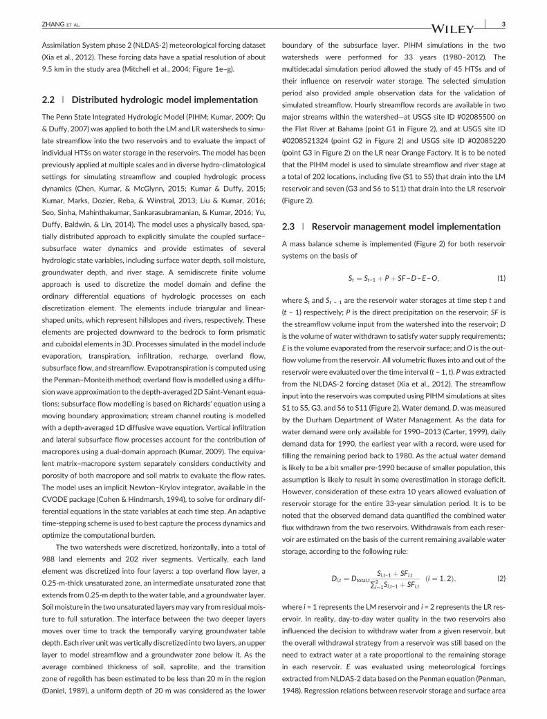
simulated streamflow. Hourly streamflow records are available in two
major streams within the watershed—at USGS site ID #02085500 on
the Flat River at Bahama (point G1 in Figure 2), and at USGS site ID
#0208521324 (point G2 in Figure 2) and USGS site ID #02085220
(point G3 in Figure 2) on the LR near Orange Factory. It is to be noted
that the PIHM model is used to simulate streamflow and river stage at
a total of 202 locations, including five (S1 to S5) that drain into the LM
reservoir and seven (G3 and S6 to S11) that drain into the LR reservoir
(Figure 2).
2.3 | Reservoir management model implementation
A mass balance scheme is implemented (Figure 2) for both reservoir
systems on the basis of
St ¼ St−1 þ Pþ SF−D−E−O; (1)
where St and St − 1 are the reservoir water storages at time step t and
(t − 1) respectively; P is the direct precipitation on the reservoir; SF is
the streamflow volume input from the watershed into the reservoir; D
is the volume of water withdrawn to satisfy water supply requirements;
E is the volume evaporated from the reservoir surface; andO is the out-
flow volume from the reservoir. All volumetric fluxes into and out of the
reservoir were evaluated over the time interval (t − 1, t). Pwas extracted
from the NLDAS‐2 forcing dataset (Xia et al., 2012). The streamflow
input into the reservoirs was computed using PIHM simulations at sites
S1 to S5, G3, and S6 to S11 (Figure 2). Water demand,D, was measured
by the Durham Department of Water Management. As the data for
water demand were only available for 1990–2013 (Carter, 1999), daily
demand data for 1990, the earliest year with a record, were used for
filling the remaining period back to 1980. As the actual water demand
is likely to be a bit smaller pre‐1990 because of smaller population, this
assumption is likely to result in some overestimation in storage deficit.
However, consideration of these extra 10 years allowed evaluation of
reservoir storage for the entire 33‐year simulation period. It is to be
noted that the observed demand data quantified the combined water
flux withdrawn from the two reservoirs. Withdrawals from each reser-
voir are estimated on the basis of the current remaining available water
storage, according to the following rule:
Di;t ¼ Dtotal;tSi;t−1 þ SFi;t
∑2i¼1Si;t−1 þ SFi;t
i ¼ 1;2ð Þ; (2)
where i = 1 represents the LM reservoir and i = 2 represents the LR res-
ervoir. In reality, day‐to‐day water quality in the two reservoirs also
influenced the decision to withdraw water from a given reservoir, but
the overall withdrawal strategy from a reservoir was still based on the
need to extract water at a rate proportional to the remaining storage
in each reservoir. E was evaluated using meteorological forcings
extracted fromNLDAS‐2 data based on the Penman equation (Penman,
1948). Regression relations between reservoir storage and surface area
FIGURE 2 Conceptual integration of LM and LR watersheds with drainage reservoirs. Watershed model, Penn State Integrated Hydrologic Model,was implemented in the two watersheds to evaluate streamflow inputs into the reservoir at 12 locations (S1 to S5, G3, and S6 to S11), whereasreservoir management model was implemented to evaluate storage and outflow from the reservoirs
4 ZHANG ET AL.
were used to calculate the evaporative surface area of each reservoir
(Carter, 1999):
ALM ¼ 0:141 SLM þ 195421:8
ALR ¼ 0:106 SLR þ 292323:5
�; (3)
where ALM is surface area of the LM reservoir and ALR is surface area of
LR reservoir in square metre, whereas storages SLM and SLR are in cubic
metres. Outflow from the reservoir, O, was simulated using reservoir
rules. For the LM reservoir, the rules mandated the following: (a) The
minimum release from the LM reservoir must be 757 m3/day between
November 1 andMay 31, and 24.2m3/day between July 1 andOctober
31; and (b) if the reservoir storage is above 70% of the working volume,
the minimum release should be 113.4 m3/day during August, and
87,065 m3/day during September and October. For the LR reservoir,
the outlet discharge used the following prescriptions: (a) Should the
reservoir storage ratio drop below 20% of the working volume, the
minimum release from the LR reservoir must be 756 m3/day; (b) should
the reservoir storage ratio be above 90% of the working volume, the
minimum release from the LR reservoir must be 15,120 m3/day; and
(c) should the reservoir storage ratio be between 20% and 90% of the
working volume, the minimum release from the LR reservoir must be
7,560 m3/day between May 1 and October 31, and 15,120 m3/day
between November 1 and April 30.
2.4 | Model parameterization, calibration, andvalidation
A geographic information system framework, PIHMgis (Bhatt, Kumar,
& Duffy, 2014), was used to automatically parameterize the
hydrogeological, ecological, and meteorological properties in the model
domain using the datasets described in Section 2.1. In both LM and LR
watersheds, PIHM simulations were performed for 33 years
(1980–2012). The calibration ofmodel parameterswas performed using
streamflow data for 2004–2012, which received a mean annual precip-
itation of 1,080 mm, the same as the average precipitation for the
entire simulation period. The calibration process involved nudging
ZHANG ET AL. 5
hydrogeological parameters uniformly across the model domain
(Refsgaard & Storm, 1996) to match the base flow magnitude and the
rate of hydrograph decay during recession. First, a PIHM simulation
was conducted by fully saturating the soil to the land surface. Themodel
was then allowed to drain with no precipitation input until streamflow
reached an approximately constant value. The simulated hydrograph
magnitude at this level state was compared with observed streamflow
during late recession periods (5 days after a streamflow peak) in the
months of April to July, the period when the streamflow is dominated
by base flow in the watershed. Next, the simulated recession rate based
on the relaxation hydrograph was compared with the observed reces-
sion rates from January to December, when the effect of evapotranspi-
ration is relatively small. The two comparisons yield calibrated
hydrogeological properties such as the van Genuchten coefficients in
the soil–water retention curves (Van Genuchten, 1980), macro and
matrix porosity and conductivity. For reference, the calibration file used
for the PIHM simulation is shown in Tables S1 and S2. Modelled and
observed water balance statistics during the calibration period
(Table 1) indicate a reliable partitioning of the water budget. The model
overpredicts the observed annual streamflow by about 16% during the
calibration period. The streamflow simulation was compared against
observations at sites G1, G2, and G3 (Figure 2) for years 1980–2012
(Figure 3a,b). Gauging station G2 provided observation data for the
period January 1, 1980, to September 30, 1987, whereas G3 provided
streamflow data for the remaining period until December 22, 2012
(Figure 3b; station G3 was installed in place of G2, which was
discontinued on September 30, 1987). Outflow, O, from the two reser-
voirs were validated at USGS site ID #02086500 located downstream
of the reservoir on Flat River and USGS site ID #0208524975 located
on the LR at Fairntosh, NC, for the years 2004 to 2012 (Figure 3c,d).
Observed and modelled storage ratios, that is, the fraction of
combined total water storage in the two reservoirs to the combined
storage capacity, for years 2004–2012 were also compared to
validate the reservoir management model simulations (Figure 3e).
Nash–Sutcliffe efficiency, the coefficient of determination (R2), root
mean square error, Pearson's correlation, and bias of streamflow and
reservoir water‐storage series (Table 2, Figure 3) show that the coupled
hydrologic and reservoir management model was able to effectively
quantify the streamflow and reservoir storage time series.
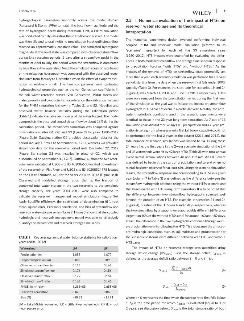
TABLE 1 Key average annual water balance statistics for calibrationyears (2004–2012)
Watershed LM LR
Precipitation (m) 1.083 1.077
Evapotranspiration (m) 0.883 0.89
Observed streamflow (m) 0.193 0.166
Simulated streamflow (m) 0.176 0.156
Observed runoff ratio 0.179 0.154
Simulated runoff ratio 0.163 0.145
RMSE (in m3/day) 6.29E+05 2.65E+05
Pearson's correlation 0.82 0.86
Bias (%) −18.33 −15.71
LM = Lake Michie watershed; LR = Little River watersheds; RMSE = rootmean square error.
2.5 | Numerical evaluation of the impact of HTSs onreservoir water storage and its theoreticalinterpretation
The numerical experiment design involved performing individual
coupled PIHM and reservoir model simulation (referred to as
“scenarios” hereafter) for each of the 33 simulation years
(1980–2012). HTS impacts were quantified by evaluating the differ-
ences in both modelled streamflow and storage time series in response
to precipitation forcings “with HTSs” and “without HTSs.” As the
impacts of the removal of HTSs on streamflow could potentially last
more than a year, each scenario simulation was performed for a 2‐year
period, starting from the date when the reservoir first falls under 100%
capacity (Table 3). For example, the start date for scenarios 19 and 24
(Figure 4) was March 11, 2004, and June 10, 2010, respectively. HTSs
were only removed from the precipitation series during the first year
of the simulation as the goal was to isolate the impact on streamflow
hydrograph if HTSs did not occur in a particular year. Notably, the ante-
cedent hydrologic conditions used in the scenario experiments were
identical to those in the 33‐year long‐term simulation. As 7 out of 33
simulation years did not receive anyHTS precipitation and a 2‐year sim-
ulation (starting fromwhen reservoirs first fall below capacity) could not
be performed for the last 2 years in the dataset (2011 and 2012), the
total number of scenario simulations was limited to 24. During these
24 years (i.e. the first years in the 2‐year scenario simulations), the LM
and LRwatershedswere hit by 42 largeHTSs (Table 3), with total annual
event rainfall accumulations between 48 and 152 mm. An HTS event
was defined to begin at the start of precipitation and to end when no
rainfall has been observed for at least 6 hr. Using the scenario simulation
results, the streamflow response size corresponding to HTSs in a given
year (column 7 in Table 3) was defined as the difference between the
streamflow hydrograph obtained using the without HTSs scenario and
that based on the with HTSs long‐term simulation. It is to be noted that
the difference between two streamflow hydrographs spanned well
beyond the duration of an HTS. For example, in scenarios 21 and 24
(Figure 4), duration of the HTS was 4 and 6 days, respectively, whereas
the two streamflow hydrographs were appreciably different (difference
larger than 10%of thewithoutHTSs case) for around 160 and 182 days.
In fact, the difference in the two hydrographs continued through multi-
ple precipitation events following the HTS. This is because the anteced-
ent hydrologic conditions, such as soil moisture and groundwater, for
the subsequent storms were different between with HTS and without
HTS cases.
The impact of HTSs on reservoir storage was quantified using
storage deficit change (ΔSdeficit). First, the storage deficit, Sdeficit, is
defined as the average deficit ratio between t = 0 and t = tD:
Sdeficit ¼ ∫tD0 1−Sratioð Þdt
tD; (4)
Sratio ¼ SLM þ SLRScapacity
; (5)
where t = 0 represents the time when the storage ratio first falls below
1, tD is the time period for which Sdeficit is evaluated (equal to 1 or
2 years, see discussion below), Sratio is the total storage ratio of both
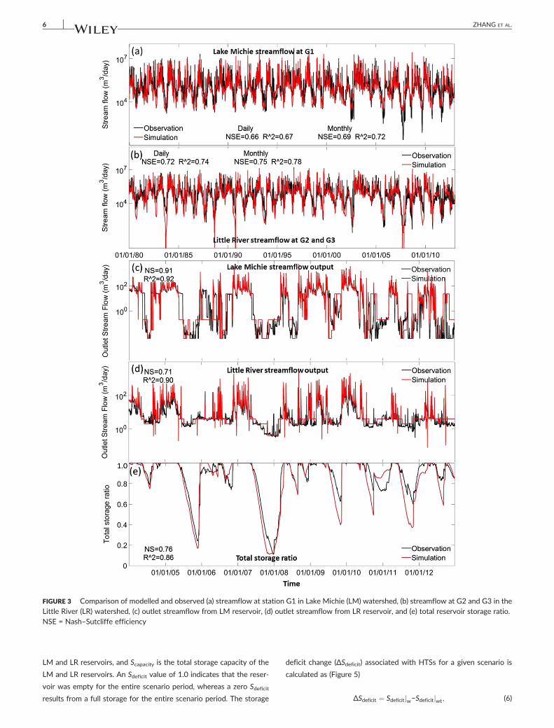
FIGURE 3 Comparison of modelled and observed (a) streamflow at station G1 in Lake Michie (LM) watershed, (b) streamflow at G2 and G3 in theLittle River (LR) watershed, (c) outlet streamflow from LM reservoir, (d) outlet streamflow from LR reservoir, and (e) total reservoir storage ratio.NSE = Nash–Sutcliffe efficiency
6 ZHANG ET AL.
LM and LR reservoirs, and Scapacity is the total storage capacity of the
LM and LR reservoirs. An Sdeficit value of 1.0 indicates that the reser-
voir was empty for the entire scenario period, whereas a zero Sdeficit
results from a full storage for the entire scenario period. The storage
deficit change (ΔSdeficit) associated with HTSs for a given scenario is
calculated as (Figure 5)
ΔSdeficit ¼ Sdeficitjw−Sdeficitjwt; (6)
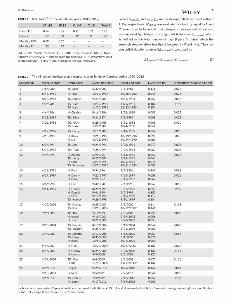
TABLE 2 NSE and R2 for the simulation years (1980–2012)
SF_LM SF_LR O_LM O_LR Total S
Daily NSE 0.66 0.72 0.91 0.71 0.76
Daily R2 .67 .74 .92 .9 .86
Monthly NSE 0.69 0.75 — — —
Monthly R2 .72 .78 — — —
LM = Lake Michie reservoir; LR = Little River reservoir; NSE = Nash–Sutcliffe efficiency; O = outflow from the reservoir; SF = streamflow inputto the reservoir; Total S = total storage in the two reservoirs.
TABLE 3 The 45 largest hurricanes and tropical storms in North Carolina
Scenario ID Scenario start Event name Event start date
1 7/6/1980 TS: Bret 6/30/1981
2 6/14/1983 H: Tico 10/22/1983
3 8/20/1984 TS: Isidore 9/27/1984
4 4/3/1985 TS: Juan 10/30/1985TS: Kate 11/20/1985
5 4/6/1986 H: Charley 8/16/1986
6 5/28/1987 TD: Nine 9/3/1987
7 3/26/1988 TD: Chris 8/28/1988TS: Isaac 10/2/1988
8 6/29/1989 TS: Barry 7/15/1989
9 6/13/1990 H: Klaus 10/10/1990H: Lili 10/21/1990
10 6/3/1991 TS: Ana 9/24/1991
11 5/12/1994 TD: Two 7/25/1994
12 4/4/1995 H: Allison 6/9/1995TD: Jerry 8/25/1995H: Opal 10/3/1995TS: Sebastien 10/20/1995
13 6/12/1996 H: Fran 9/3/1996
14 6/17/1997 H: Danny 7/22/1997H: Erika 9/9/1997
15 6/6/1998 H: Earl 9/3/1998
16 5/11/1999 H: Dennis 8/25/1999H: Dennis 9/4/1999H: Floyd 9/14/1999TS: Harvey 9/26/1999
17 4/20/2001 TS: Gustav 8/25/2002TS: Kyle 10/10/2002
18 7/1/2003 TD: Bill 7/1/2003H: Isabel 9/18/2003H: Juan 9/22/2003
19 3/10/2004 TS: Bonnie 8/13/2004TD: Gaston 8/29/2004
20 3/1/2006 TS: Alberto 6/13/2006TS: Ernesto 8/30/2006H: Isaac 10/5/2006
21 5/1/2007 H: Noel 10/24/2007
22 6/1/2008 H: Gustav 8/25/2008H: Hanna 9/5/2008
23 4/27/2009 TD: One 6/4/2009H: Ida 11/10/2009
24 6/9/2010 H: Igor 9/26/2010
— 5/18/2011 H: Irene 9/5/2011
— 6/1/2012 TS: Debby 7/9/2012H: Sandy 9/17/2012
Each scenario represents a 2‐year simulation experiment. Definitions of TS, TD,ricane; TD = tropical depression; TS = tropical storm.
ZHANG ET AL. 7
where Sdeficit|w and Sdeficit|wt are the storage deficits with and without
HTSs, respectively. ΔSdeficit was evaluated for both tD equal to 1 and
2 years. It is to be noted that changes in storage deficit are also
accompanied by changes in storage deficit duration (Sduration), which
is defined as the total number of days (Figure 5) during which the
reservoir storage ratio is less than 1 between t = 0 and t = tD. The stor-
age deficit duration change (ΔSduration) is calculated as
ΔSduration ¼ Sdurationjwt−Sdurationjw; (7)
during 1980–2012
Event end date Event size (m) Streamflow response size (m)
7/6/1981 0.116 0.027
10/26/1983 0.048 0.025
10/2/1984 0.052 0.018
11/5/1985 0.109 0.14711/23/1985 0.104
8/22/1986 0.093 0.023
9/8/1987 0.098 0.023
8/31/1988 0.068 0.03010/4/1988 0.061
7/18/1989 0.052 0.013
10/13/1990 0.099 0.08510/24/1990 0.083
9/26/1991 0.077 0.028
7/29/1994 0.063 0.008
6/13/1995 0.052 0.0958/28/1995 0.06610/6/1995 0.07510/21/1995 0.053
9/7/1996 0.145 0.081
7/25/1997 0.058 0.0269/11/1997 0.062
9/4/1998 0.069 0.015
8/27/1999 0.055 0.2379/7/1999 0.1529/16/1999 0.1179/30/1999 0.104
9/3/2002 0.114 0.13510/12/2002 0.141
7/3/2003 0.055 0.0609/19/2003 0.0569/23/2003 0.053
8/17/2004 0.064 0.0438/31/2004 0.061
6/14/2006 0.053 0.0589/1/2006 0.07410/7/2006 0.051
10/27/2007 0.102 0.027
8/28/2008 0.132 0.1219/6/2008 0.125
6/5/2009 0.070 0.13011/14/2009 0.139
10/1/2010 0.142 0.041
9/7/2011 0.064 0.012
7/11/2012 0.057 0.1069/19/2012 0.063
and H are available at http://www.nhc.noaa.gov/aboutgloss.shtml. H = hur-
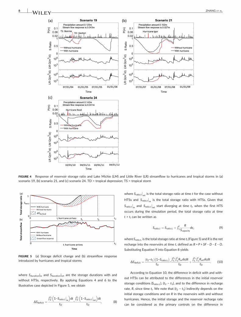
FIGURE 4 Response of reservoir storage ratio and Lake Michie (LM) and Little River (LR) streamflow to hurricanes and tropical storms in (a)scenario 19, (b) scenario 21, and (c) scenario 24. TD = tropical depression; TS = tropical storm
FIGURE 5 (a) Storage deficit change and (b) streamflow responseintroduced by hurricanes and tropical storms
8 ZHANG ET AL.
where Sduration|w and Sduration|wt are the storage durations with and
without HTSs, respectively. By applying Equations 4 and 6 to the
illustrative case depicted in Figure 5, we obtain
ΔSdeficit ¼∫t20 1−Sratio;t
��w
� �dt
tD−∫t10 1−Sratio;t
��wt
� �dt
tD; (8)
where Sratio;t��wt
is the total storage ratio at time t for the case without
HTSs and Sratio;t��w is the total storage ratio with HTSs. Given that
Sratio;t��w and Sratio;t
��wt start diverging at time ti, when the first HTS
occurs during the simulation period, the total storage ratio at time
t > ti can be written as
Sratio;t ¼ Sratio;ti þ ∫tti
RScapacity
dϛ; (9)
whereSratio;ti is the total storage ratio at time ti (Figure 5) and R is the net
recharge into the reservoirs at time t, defined as R = P + SF −D − E −O.
Substituting Equation 9 into Equation 8 yields
ΔSdeficit ¼t2−t1ð Þ 1−Sratio;ti
� �tD
−∫t2ti∫ttiRwdϛdttD
þ ∫t1ti∫ttiRwtdϛdttD
: (10)
According to Equation 10, the difference in deficit with and with-
out HTSs can be attributed to the differences in the initial reservoir
storage conditions (Sratio;ti ), (t2 − t1), and to the difference in recharge
rate, R, since time ti. We note that (t2 − t1) indirectly depends on the
initial storage conditions and on R in the reservoirs with and without
hurricanes. Hence, the initial storage and the reservoir recharge rate
can be considered as the primary controls on the difference in
ZHANG ET AL. 9
storage deficit. As the recharge rate, R, is a function of P, SF, D, E,
and O (see definitions of variables used in Equation 9), the differ-
ence in any of these variables after an HTS can lead to a difference
in storage deficit change.
3 | RESULTS AND DISCUSSION
3.1 | Role of HTSs on storage in water‐supplyreservoirs
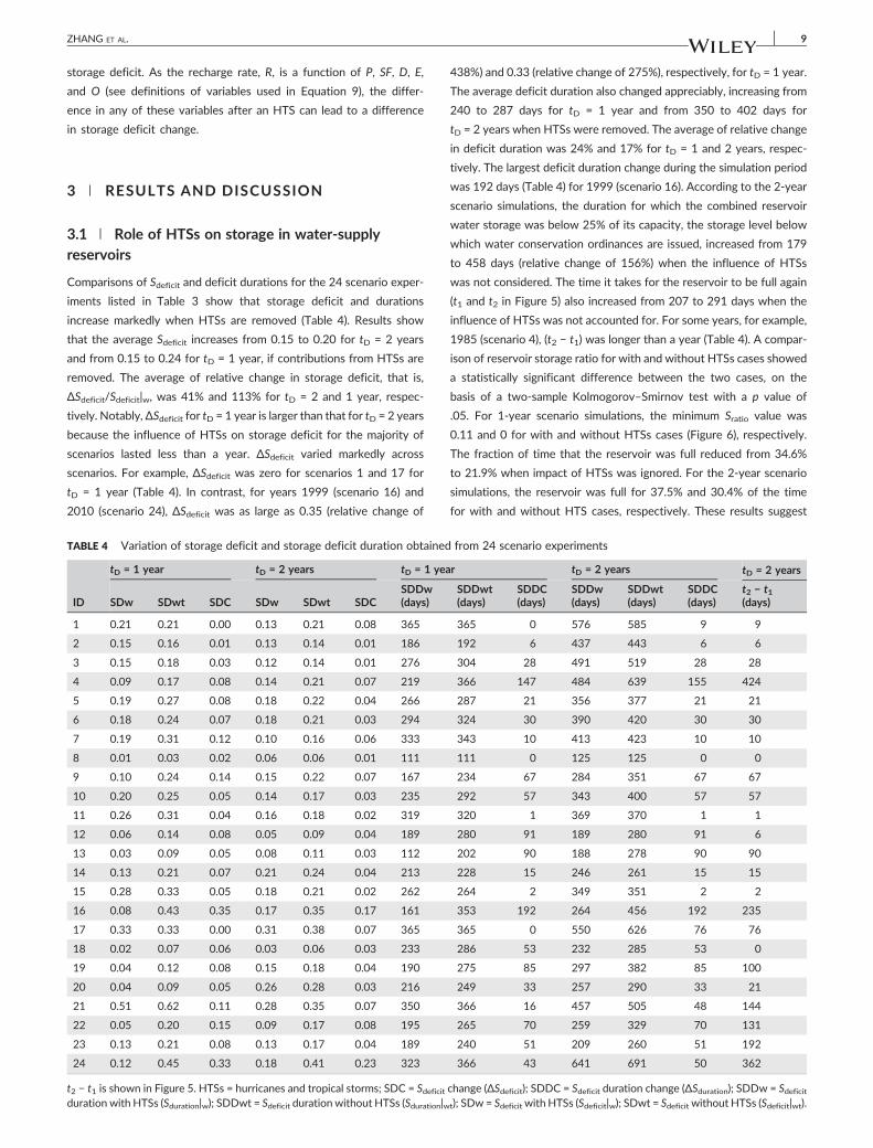
Comparisons of Sdeficit and deficit durations for the 24 scenario exper-
iments listed in Table 3 show that storage deficit and durations
increase markedly when HTSs are removed (Table 4). Results show
that the average Sdeficit increases from 0.15 to 0.20 for tD = 2 years
and from 0.15 to 0.24 for tD = 1 year, if contributions from HTSs are
removed. The average of relative change in storage deficit, that is,
ΔSdeficit/Sdeficit|w, was 41% and 113% for tD = 2 and 1 year, respec-
tively. Notably, ΔSdeficit for tD = 1 year is larger than that for tD = 2 years
because the influence of HTSs on storage deficit for the majority of
scenarios lasted less than a year. ΔSdeficit varied markedly across
scenarios. For example, ΔSdeficit was zero for scenarios 1 and 17 for
tD = 1 year (Table 4). In contrast, for years 1999 (scenario 16) and
2010 (scenario 24), ΔSdeficit was as large as 0.35 (relative change of
TABLE 4 Variation of storage deficit and storage deficit duration obtained
ID
tD = 1 year tD = 2 years tD = 1 yea
SDw SDwt SDC SDw SDwt SDCSDDw(days)
1 0.21 0.21 0.00 0.13 0.21 0.08 365
2 0.15 0.16 0.01 0.13 0.14 0.01 186
3 0.15 0.18 0.03 0.12 0.14 0.01 276
4 0.09 0.17 0.08 0.14 0.21 0.07 219
5 0.19 0.27 0.08 0.18 0.22 0.04 266
6 0.18 0.24 0.07 0.18 0.21 0.03 294
7 0.19 0.31 0.12 0.10 0.16 0.06 333
8 0.01 0.03 0.02 0.06 0.06 0.01 111
9 0.10 0.24 0.14 0.15 0.22 0.07 167
10 0.20 0.25 0.05 0.14 0.17 0.03 235
11 0.26 0.31 0.04 0.16 0.18 0.02 319
12 0.06 0.14 0.08 0.05 0.09 0.04 189
13 0.03 0.09 0.05 0.08 0.11 0.03 112
14 0.13 0.21 0.07 0.21 0.24 0.04 213
15 0.28 0.33 0.05 0.18 0.21 0.02 262
16 0.08 0.43 0.35 0.17 0.35 0.17 161
17 0.33 0.33 0.00 0.31 0.38 0.07 365
18 0.02 0.07 0.06 0.03 0.06 0.03 233
19 0.04 0.12 0.08 0.15 0.18 0.04 190
20 0.04 0.09 0.05 0.26 0.28 0.03 216
21 0.51 0.62 0.11 0.28 0.35 0.07 350
22 0.05 0.20 0.15 0.09 0.17 0.08 195
23 0.13 0.21 0.08 0.13 0.17 0.04 189
24 0.12 0.45 0.33 0.18 0.41 0.23 323
t2 − t1 is shown in Figure 5. HTSs = hurricanes and tropical storms; SDC = Sdeficitduration with HTSs (Sduration|w); SDDwt = Sdeficit duration without HTSs (Sduration|w
438%) and 0.33 (relative change of 275%), respectively, for tD = 1 year.
The average deficit duration also changed appreciably, increasing from
240 to 287 days for tD = 1 year and from 350 to 402 days for
tD = 2 years when HTSs were removed. The average of relative change
in deficit duration was 24% and 17% for tD = 1 and 2 years, respec-
tively. The largest deficit duration change during the simulation period
was 192 days (Table 4) for 1999 (scenario 16). According to the 2‐year
scenario simulations, the duration for which the combined reservoir
water storage was below 25% of its capacity, the storage level below
which water conservation ordinances are issued, increased from 179
to 458 days (relative change of 156%) when the influence of HTSs
was not considered. The time it takes for the reservoir to be full again
(t1 and t2 in Figure 5) also increased from 207 to 291 days when the
influence of HTSs was not accounted for. For some years, for example,
1985 (scenario 4), (t2 − t1) was longer than a year (Table 4). A compar-
ison of reservoir storage ratio for with and without HTSs cases showed
a statistically significant difference between the two cases, on the
basis of a two‐sample Kolmogorov–Smirnov test with a p value of
.05. For 1‐year scenario simulations, the minimum Sratio value was
0.11 and 0 for with and without HTSs cases (Figure 6), respectively.
The fraction of time that the reservoir was full reduced from 34.6%
to 21.9% when impact of HTSs was ignored. For the 2‐year scenario
simulations, the reservoir was full for 37.5% and 30.4% of the time
for with and without HTS cases, respectively. These results suggest
from 24 scenario experiments
r tD = 2 years tD = 2 years
SDDwt(days)
SDDC(days)
SDDw(days)
SDDwt(days)
SDDC(days)
t2 − t1(days)
365 0 576 585 9 9
192 6 437 443 6 6
304 28 491 519 28 28
366 147 484 639 155 424
287 21 356 377 21 21
324 30 390 420 30 30
343 10 413 423 10 10
111 0 125 125 0 0
234 67 284 351 67 67
292 57 343 400 57 57
320 1 369 370 1 1
280 91 189 280 91 6
202 90 188 278 90 90
228 15 246 261 15 15
264 2 349 351 2 2
353 192 264 456 192 235
365 0 550 626 76 76
286 53 232 285 53 0
275 85 297 382 85 100
249 33 257 290 33 21
366 16 457 505 48 144
265 70 259 329 70 131
240 51 209 260 51 192
366 43 641 691 50 362
change (ΔSdeficit); SDDC = Sdeficit duration change (ΔSduration); SDDw = Sdeficitt); SDw = Sdeficit with HTSs (Sdeficit|w); SDwt = Sdeficit without HTSs (Sdeficit|wt).
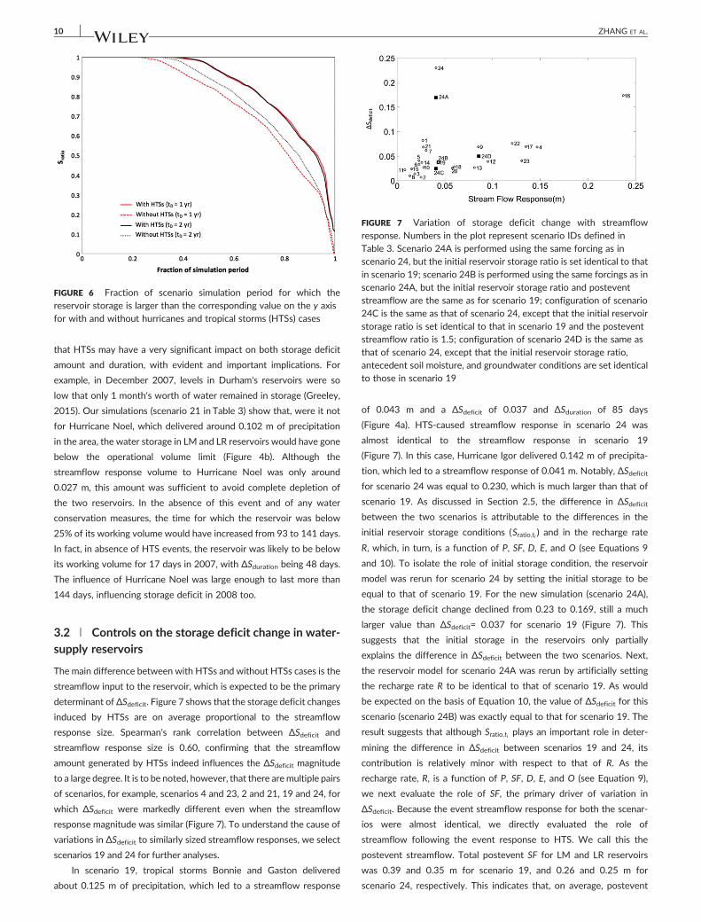
FIGURE 6 Fraction of scenario simulation period for which thereservoir storage is larger than the corresponding value on the y axisfor with and without hurricanes and tropical storms (HTSs) cases
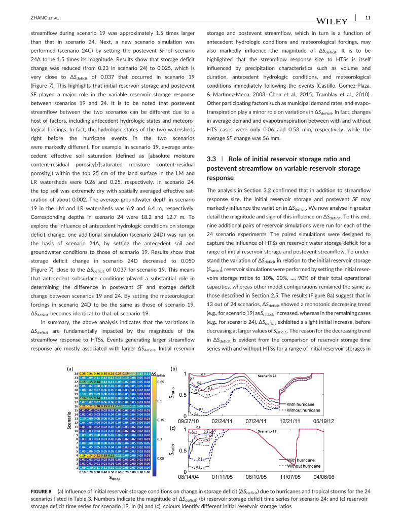
FIGURE 7 Variation of storage deficit change with streamflowresponse. Numbers in the plot represent scenario IDs defined inTable 3. Scenario 24A is performed using the same forcing as inscenario 24, but the initial reservoir storage ratio is set identical to thatin scenario 19; scenario 24B is performed using the same forcings as inscenario 24A, but the initial reservoir storage ratio and posteventstreamflow are the same as for scenario 19; configuration of scenario24C is the same as that of scenario 24, except that the initial reservoirstorage ratio is set identical to that in scenario 19 and the posteventstreamflow ratio is 1.5; configuration of scenario 24D is the same asthat of scenario 24, except that the initial reservoir storage ratio,antecedent soil moisture, and groundwater conditions are set identicalto those in scenario 19
10 ZHANG ET AL.
that HTSs may have a very significant impact on both storage deficit
amount and duration, with evident and important implications. For
example, in December 2007, levels in Durham's reservoirs were so
low that only 1 month's worth of water remained in storage (Greeley,
2015). Our simulations (scenario 21 in Table 3) show that, were it not
for Hurricane Noel, which delivered around 0.102 m of precipitation
in the area, the water storage in LM and LR reservoirs would have gone
below the operational volume limit (Figure 4b). Although the
streamflow response volume to Hurricane Noel was only around
0.027 m, this amount was sufficient to avoid complete depletion of
the two reservoirs. In the absence of this event and of any water
conservation measures, the time for which the reservoir was below
25% of its working volume would have increased from 93 to 141 days.
In fact, in absence of HTS events, the reservoir was likely to be below
its working volume for 17 days in 2007, with ΔSduration being 48 days.
The influence of Hurricane Noel was large enough to last more than
144 days, influencing storage deficit in 2008 too.
3.2 | Controls on the storage deficit change in water‐supply reservoirs
The main difference between with HTSs and without HTSs cases is the
streamflow input to the reservoir, which is expected to be the primary
determinant of ΔSdeficit. Figure 7 shows that the storage deficit changes
induced by HTSs are on average proportional to the streamflow
response size. Spearman's rank correlation between ΔSdeficit and
streamflow response size is 0.60, confirming that the streamflow
amount generated by HTSs indeed influences the ΔSdeficit magnitude
to a large degree. It is to be noted, however, that there aremultiple pairs
of scenarios, for example, scenarios 4 and 23, 2 and 21, 19 and 24, for
which ΔSdeficit were markedly different even when the streamflow
response magnitude was similar (Figure 7). To understand the cause of
variations in ΔSdeficit to similarly sized streamflow responses, we select
scenarios 19 and 24 for further analyses.
In scenario 19, tropical storms Bonnie and Gaston delivered
about 0.125 m of precipitation, which led to a streamflow response
of 0.043 m and a ΔSdeficit of 0.037 and ΔSduration of 85 days
(Figure 4a). HTS‐caused streamflow response in scenario 24 was
almost identical to the streamflow response in scenario 19
(Figure 7). In this case, Hurricane Igor delivered 0.142 m of precipita-
tion, which led to a streamflow response of 0.041 m. Notably, ΔSdeficitfor scenario 24 was equal to 0.230, which is much larger than that of
scenario 19. As discussed in Section 2.5, the difference in ΔSdeficitbetween the two scenarios is attributable to the differences in the
initial reservoir storage conditions (Sratio;ti ) and in the recharge rate
R, which, in turn, is a function of P, SF, D, E, and O (see Equations 9
and 10). To isolate the role of initial storage condition, the reservoir
model was rerun for scenario 24 by setting the initial storage to be
equal to that of scenario 19. For the new simulation (scenario 24A),
the storage deficit change declined from 0.23 to 0.169, still a much
larger value than ΔSdeficit= 0.037 for scenario 19 (Figure 7). This
suggests that the initial storage in the reservoirs only partially
explains the difference in ΔSdeficit between the two scenarios. Next,
the reservoir model for scenario 24A was rerun by artificially setting
the recharge rate R to be identical to that of scenario 19. As would
be expected on the basis of Equation 10, the value of ΔSdeficit for this
scenario (scenario 24B) was exactly equal to that for scenario 19. The
result suggests that although Sratio;ti plays an important role in deter-
mining the difference in ΔSdeficit between scenarios 19 and 24, its
contribution is relatively minor with respect to that of R. As the
recharge rate, R, is a function of P, SF, D, E, and O (see Equation 9),
we next evaluate the role of SF, the primary driver of variation in
ΔSdeficit. Because the event streamflow response for both the scenar-
ios were almost identical, we directly evaluated the role of
streamflow following the event response to HTS. We call this the
postevent streamflow. Total postevent SF for LM and LR reservoirs
was 0.39 and 0.35 m for scenario 19, and 0.26 and 0.25 m for
scenario 24, respectively. This indicates that, on average, postevent
ZHANG ET AL. 11
streamflow during scenario 19 was approximately 1.5 times larger
than that in scenario 24. Next, a new scenario simulation was
performed (scenario 24C) by setting the postevent SF of scenario
24A to be 1.5 times its magnitude. Results show that storage deficit
change was reduced (from 0.23 in scenario 24) to 0.025, which is
very close to ΔSdeficit of 0.037 that occurred in scenario 19
(Figure 7). This highlights that initial reservoir storage and postevent
SF played a major role in the variable reservoir storage response
between scenarios 19 and 24. It is to be noted that postevent
streamflow between the two scenarios can be different due to a
host of factors, including antecedent hydrologic states and meteoro-
logical forcings. In fact, the hydrologic states of the two watersheds
right before the hurricane events in the two scenarios
were markedly different. For example, in scenario 19, average ante-
cedent effective soil saturation (defined as [absolute moisture
content‐residual porosity]/[saturated moisture content‐residual
porosity]) within the top 25 cm of the land surface in the LM and
LR watersheds were 0.26 and 0.25, respectively. In scenario 24,
the top soil was extremely dry with spatially averaged effective sat-
uration of about 0.002. The average groundwater depth in scenario
19 in the LM and LR watersheds was 6.9 and 6.4 m, respectively.
Corresponding depths in scenario 24 were 18.2 and 12.7 m. To
explore the influence of antecedent hydrologic conditions on storage
deficit change, one additional simulation (scenario 24D) was run on
the basis of scenario 24A, by setting the antecedent soil and
groundwater conditions to those of scenario 19. Results show that
storage deficit change in scenario 24D decreased to 0.050
(Figure 7), close to the ΔSdeficit of 0.037 for scenario 19. This means
that antecedent subsurface conditions played a substantial role in
determining the difference in postevent SF and storage deficit
change between scenarios 19 and 24. By setting the meteorological
forcings in scenario 24D to be the same as those of scenario 19,
ΔSdeficit becomes identical to that of scenario 19.
In summary, the above analysis indicates that the variations in
ΔSdeficit are fundamentally impacted by the magnitude of the
streamflow response to HTSs. Events generating larger streamflow
response are mostly associated with larger ΔSdeficit. Initial reservoir
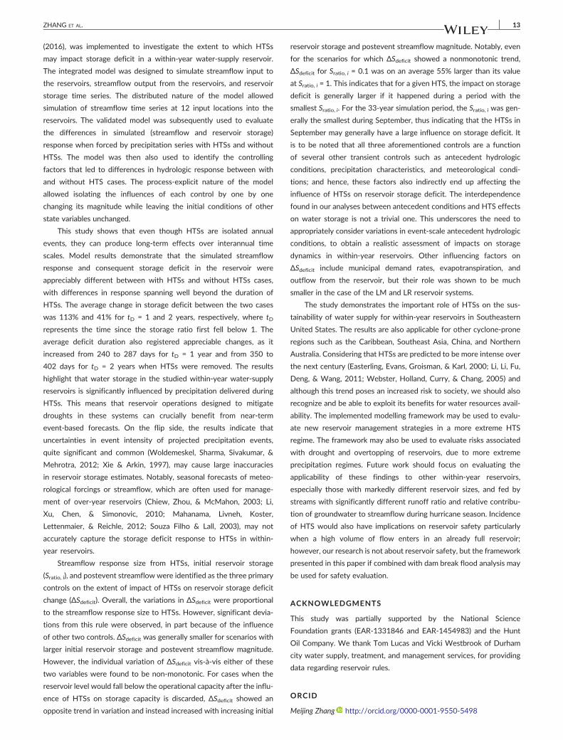
FIGURE 8 (a) Influence of initial reservoir storage conditions on change in sscenarios listed in Table 3. Numbers indicate the magnitude of ΔSdeficit; (b)storage deficit time series for scenario 19. In (b) and (c), colours identify di
storage and postevent streamflow, which in turn is a function of
antecedent hydrologic conditions and meteorological forcings, may
also markedly influence the magnitude of ΔSdeficit. It is to be
highlighted that the streamflow response size to HTSs is itself
influenced by precipitation characteristics such as volume and
duration, antecedent hydrologic conditions, and meteorological
conditions immediately following the events (Castillo, Gomez‐Plaza,
& Martınez‐Mena, 2003; Chen et al., 2015; Tramblay et al., 2010).
Other participating factors such as municipal demand rates, and evapo-
transpiration play a minor role on variations in ΔSdeficit. In fact, changes
in average demand and evapotranspiration between with and without
HTS cases were only 0.06 and 0.53 mm, respectively, while the
average SF change was 56 mm.
3.3 | Role of initial reservoir storage ratio andpostevent streamflow on variable reservoir storageresponse
The analysis in Section 3.2 confirmed that in addition to streamflow
response size, the initial reservoir storage and postevent SF may
markedly influence the variation in ΔSdeficit. We now analyse in greater
detail the magnitude and sign of this influence on ΔSdeficit. To this end,
nine additional pairs of reservoir simulations were run for each of the
24 scenario experiments. The paired simulations were designed to
capture the influence of HTSs on reservoir water storage deficit for a
range of initial reservoir storage and postevent streamflow. To under-
stand the variation of ΔSdeficit in relation to the initial reservoir storage
(Sratio,i), reservoir simulationswere performed by setting the initial reser-
voirs storage ratios to 10%, 20%, …, 90% of their total operational
capacities, whereas other model configurations remained the same as
those described in Section 2.5. The results (Figure 8a) suggest that in
13 out of 24 scenarios, ΔSdeficit showed a monotonic decreasing trend
(e.g., for scenario 19) asSratio;ti increased, whereas in the remaining cases
(e.g., for scenario 24), ΔSdeficit exhibited a slight initial increase, before
decreasing at larger values ofSratio;ti . The reason for the decreasing trend
in ΔSdeficit is evident from the comparison of reservoir storage time
series with and without HTSs for a range of initial reservoir storages in
torage deficit (ΔSdeficit) due to hurricanes and tropical storms for the 24reservoir storage deficit time series for scenario 24; and (c) reservoirfferent initial reservoir storage ratios

FIGURE 9 Influence of postevent streamflow on the change in storage deficit (ΔSdeficit) due to hurricanes and tropical storms for the 24 scenarioslisted inTable 3, when (a) initial storage ratio is 10%, (b) initial storage ratio is 50%, and (c) initial storage ratio is 90%; (d) storage ratio time series forscenario 24 with initial storage ratio of 10%. Numbers in (a)–(c) indicate the magnitude of ΔSdeficit. Colours in (d) identify different ratios ofpostevent streamflow
12 ZHANG ET AL.
Figure 8c. As Sratio;ti increases, so is the increase in both Sratio;t��wand
Sratio;t��wt. However, for larger values of Sratio;ti (e.g., Sratio, i equal to 0.7
or 0.9 in Figure 8c), Sratio;t��wis equal to its ceiling value of 1 for a longer
period and, hence, does not increase as much as Sratio;t��wt. As a result,
ΔSdeficit decreases with increasing Sratio;ti . For the scenarios exhibiting
a nonmonotonic trend (e.g., scenario 24 in Figure 8a and8b),ΔSdeficit still
increaseswith decrease inSratio;ti until a certain threshold value ofSratio;ti
is reached. For example, the threshold Sratio;ti for scenario 24 is 0.3.
However, below this threshold, ΔSdeficit decreases with a decrease in
Sratio;ti . The reason for this reversal in the trend of ΔSdeficit is evident
from the comparison of reservoir storage time series in Figure 8b. For
smaller values of Sratio;ti (e.g., Sratio, i equal to 0.1 in Figure 8b), Sratio;t��wt
becomes zero, indicating that the reservoir level has fallen below its
operating capacity when the HTSs are removed. With a further
decrease in Sratio;ti , Sratio;t��wt is equal to zero for a longer period of time,
and hence, Sratio;t��wt does not decrease as much as Sratio;t
��w. As a result,
ΔSdeficit decreases with decrease in initial reservoir ratio below a certain
Sratio;ti threshold, thereby resulting in a nonmonotonic trend in ΔSdeficit.
Notably, even for the 11 scenarios for which ΔSdeficit showed a
nonmonotonic trend, ΔSdeficit for (Sratio, i = 0.1) was on an average 55%
larger than its value at (Sratio, i = 1) was. For 12 out of 13 scenarios for
which ΔSdeficit decreased monotonically with increase in Sratio, i, ΔSdeficitfor Sratio, i = 0.1 was on an average 485% larger than its value at Sratio,
i = 1was. These results indicate that for a givenHTS, the impact on stor-
age deficit is generally larger if it happened during a period with the
smallest Sratio, i. For the 33‐year simulation period, the Sratio, i was
generally the smallest during September, thus indicating the HTSs in
September may generally have a large influence on storage deficit.
To investigate the variation in ΔSdeficit vis‐à‐vis postevent SF mag-
nitude, nine reservoir simulations were performed for each of the 24
scenarios by setting the postevent streamflow SF to be 0.6, 0.7, …,
1.4, 1.5 times the SF from the reference simulation. The remaining
model configurations, such as the HTS‐generated streamflow
response, initial reservoir storage ratios, and meteorological forcings,
remained the same. The relationship between the storage deficit
change and the postevent SF is shown in Figure 9a–c, for Sratio;ti equal
to 10%, 50%, and 90% of total storage capacity, respectively. ΔSdeficitagain decreased with increasing postevent streamflow in some scenar-
ios and showed an initial increase followed by a subsequent decline in
others. The expressed trends can again be explained on the basis of the
logic presented earlier. For relatively large postevent SF, the likelihood
of Sratio;t��wto be equal to 1 increases, thus limiting its rate of increase
with postevent SF. This results in a decrease in ΔSdeficit with increase in
postevent SF. However, below a threshold postevent SF magnitude,
ΔSdeficit decreases with postevent SF as the reservoir is likely to be
empty for a longer time if HTSs are removed, such that Sratio;t��wt
does
not decrease as much as Sratio;t��w(Figure 9d).
4 | SUMMARY AND CONCLUSIONS
An integrated watershed and reservoir management model, in the
same vein as one presented by Zhao, Gao, Naz, Kao, and Voisin
ZHANG ET AL. 13
(2016), was implemented to investigate the extent to which HTSs
may impact storage deficit in a within‐year water‐supply reservoir.
The integrated model was designed to simulate streamflow input to
the reservoirs, streamflow output from the reservoirs, and reservoir
storage time series. The distributed nature of the model allowed
simulation of streamflow time series at 12 input locations into the
reservoirs. The validated model was subsequently used to evaluate
the differences in simulated (streamflow and reservoir storage)
response when forced by precipitation series with HTSs and without
HTSs. The model was then also used to identify the controlling
factors that led to differences in hydrologic response between with
and without HTS cases. The process‐explicit nature of the model
allowed isolating the influences of each control by one by one
changing its magnitude while leaving the initial conditions of other
state variables unchanged.
This study shows that even though HTSs are isolated annual
events, they can produce long‐term effects over interannual time
scales. Model results demonstrate that the simulated streamflow
response and consequent storage deficit in the reservoir were
appreciably different between with HTSs and without HTSs cases,
with differences in response spanning well beyond the duration of
HTSs. The average change in storage deficit between the two cases
was 113% and 41% for tD = 1 and 2 years, respectively, where tD
represents the time since the storage ratio first fell below 1. The
average deficit duration also registered appreciable changes, as it
increased from 240 to 287 days for tD = 1 year and from 350 to
402 days for tD = 2 years when HTSs were removed. The results
highlight that water storage in the studied within‐year water‐supply
reservoirs is significantly influenced by precipitation delivered during
HTSs. This means that reservoir operations designed to mitigate
droughts in these systems can crucially benefit from near‐term
event‐based forecasts. On the flip side, the results indicate that
uncertainties in event intensity of projected precipitation events,
quite significant and common (Woldemeskel, Sharma, Sivakumar, &
Mehrotra, 2012; Xie & Arkin, 1997), may cause large inaccuracies
in reservoir storage estimates. Notably, seasonal forecasts of meteo-
rological forcings or streamflow, which are often used for manage-
ment of over‐year reservoirs (Chiew, Zhou, & McMahon, 2003; Li,
Xu, Chen, & Simonovic, 2010; Mahanama, Livneh, Koster,
Lettenmaier, & Reichle, 2012; Souza Filho & Lall, 2003), may not
accurately capture the storage deficit response to HTSs in within‐
year reservoirs.
Streamflow response size from HTSs, initial reservoir storage
(Sratio, i), and postevent streamflow were identified as the three primary
controls on the extent of impact of HTSs on reservoir storage deficit
change (ΔSdeficit). Overall, the variations in ΔSdeficit were proportional
to the streamflow response size to HTSs. However, significant devia-
tions from this rule were observed, in part because of the influence
of other two controls. ΔSdeficit was generally smaller for scenarios with
larger initial reservoir storage and postevent streamflow magnitude.
However, the individual variation of ΔSdeficit vis‐à‐vis either of these
two variables were found to be non‐monotonic. For cases when the
reservoir level would fall below the operational capacity after the influ-
ence of HTSs on storage capacity is discarded, ΔSdeficit showed an
opposite trend in variation and instead increased with increasing initial
reservoir storage and postevent streamflow magnitude. Notably, even
for the scenarios for which ΔSdeficit showed a nonmonotonic trend,
ΔSdeficit for Sratio, i = 0.1 was on an average 55% larger than its value
at Sratio, i = 1. This indicates that for a given HTS, the impact on storage
deficit is generally larger if it happened during a period with the
smallest Sratio, i. For the 33‐year simulation period, the Sratio, i was gen-
erally the smallest during September, thus indicating that the HTSs in
September may generally have a large influence on storage deficit. It
is to be noted that all three aforementioned controls are a function
of several other transient controls such as antecedent hydrologic
conditions, precipitation characteristics, and meteorological condi-
tions; and hence, these factors also indirectly end up affecting the
influence of HTSs on reservoir storage deficit. The interdependence
found in our analyses between antecedent conditions and HTS effects
on water storage is not a trivial one. This underscores the need to
appropriately consider variations in event‐scale antecedent hydrologic
conditions, to obtain a realistic assessment of impacts on storage
dynamics in within‐year reservoirs. Other influencing factors on
ΔSdeficit include municipal demand rates, evapotranspiration, and
outflow from the reservoir, but their role was shown to be much
smaller in the case of the LM and LR reservoir systems.
The study demonstrates the important role of HTSs on the sus-
tainability of water supply for within‐year reservoirs in Southeastern
United States. The results are also applicable for other cyclone‐prone
regions such as the Caribbean, Southeast Asia, China, and Northern
Australia. Considering that HTSs are predicted to be more intense over
the next century (Easterling, Evans, Groisman, & Karl, 2000; Li, Li, Fu,
Deng, & Wang, 2011; Webster, Holland, Curry, & Chang, 2005) and
although this trend poses an increased risk to society, we should also
recognize and be able to exploit its benefits for water resources avail-
ability. The implemented modelling framework may be used to evalu-
ate new reservoir management strategies in a more extreme HTS
regime. The framework may also be used to evaluate risks associated
with drought and overtopping of reservoirs, due to more extreme
precipitation regimes. Future work should focus on evaluating the
applicability of these findings to other within‐year reservoirs,
especially those with markedly different reservoir sizes, and fed by
streams with significantly different runoff ratio and relative contribu-
tion of groundwater to streamflow during hurricane season. Incidence
of HTS would also have implications on reservoir safety particularly
when a high volume of flow enters in an already full reservoir;
however, our research is not about reservoir safety, but the framework
presented in this paper if combined with dam break flood analysis may
be used for safety evaluation.
ACKNOWLEDGMENTS
This study was partially supported by the National Science
Foundation grants (EAR‐1331846 and EAR‐1454983) and the Hunt
Oil Company. We thank Tom Lucas and Vicki Westbrook of Durham
city water supply, treatment, and management services, for providing
data regarding reservoir rules.
ORCID
Meijing Zhang http://orcid.org/0000-0001-9550-5498
14 ZHANG ET AL.
REFERENCES
Anderson, J., Chung, F., Anderson, M., Brekke, L., Easton, D., Ejeta, M., …Snyder, R. (2008). Progress on incorporating climate change into man-agement of California's water resources. Climatic Change, 87, 91–108.
Ashley, S. T., & Ashley, W. S. (2008). Flood fatalities in the United States.Journal of Applied Meteorology and Climatology, 47, 805–818.
Bhatt, G., Kumar, M., & Duffy, C. J. (2014). A tightly coupled GIS anddistributed hydrologic modeling framework. Environmental Modelling &Software, 62, 70–84.
Carpenter, T. M., & Georgakakos, K. P. (2001). Assessment of Folsom lakeresponse to historical and potential future climate scenarios: 1.Forecasting. Journal of Hydrology, 249, 148–175.
Carter, S. (1999). A risk‐based simulation model for drought management inDurham, North Carolina. University of North Carolina at Chapel Hill.
Castillo, V., Gomez‐Plaza, A., & Martınez‐Mena, M. (2003). The role of ante-cedent soil water content in the runoff response of semiaridcatchments: A simulation approach. Journal of Hydrology, 284,114–130.
Changnon, S. A. (2009). Characteristics of severe Atlantic hurricanes in theUnited States: 1949–2006. Natural Hazards, 48, 329–337.
Chen, X., Kumar, M., & McGlynn, B. L. (2015). Variations in streamflowresponse to large hurricane‐season storms in a Southeastern USwatershed. Journal of Hydrometeorology, 16, 55–69.
Chiew, F., Zhou, S., & McMahon, T. (2003). Use of seasonal streamflowforecasts in water resources management. Journal of Hydrology, 270,135–144.
Chowdhury, N. T. (2010). Water management in Bangladesh: An analyticalreview. Water Policy, 12, 32–51.
Chu, G., Liu, J., Sun, Q., Lu, H., Gu, Z., Wang, W., & Liu, T. (2002). The‘mediaeval warm period’ drought recorded in Lake Huguangyan, tropi-cal South China. The Holocene, 12, 511–516.
Cohen, S. D., & Hindmarsh, A. C. (1994). CVODE user guide. TechnicalReport UCRL‐MA‐118618, LLNL.
Dale, V. H., Joyce, L. A., McNulty, S., Neilson, R. P., Ayres, M. P., Flannigan,M. D., … Peterson, C. J. (2001). Climate change and forest disturbances:Climate change can affect forests by altering the frequency, intensity,duration, and timing of fire, drought, introduced species, insect andpathogen outbreaks, hurricanes, windstorms, ice storms, or landslides.Bioscience, 51, 723–734.
Daniel, C. C. (1989). Statistical analysis relating well yield to constructionpractices and siting of wells in the Piedmont and Blue Ridge Provincesof North Carolina. USGPO; for sale by the books and open‐file reportssection, US Geological Survey.
Easterling, D. R., Evans, J., Groisman, P. Y., & Karl, T. (2000). Observedvariability and trends in extreme climate events: A brief review. Bulletinof the American Meteorological Society, 81, 417.
Elsner, J. B. (2007). Granger causality and Atlantic hurricanes. Tellus A, 59,476–485.
Emanuel, K., Sundararajan, R., & Williams, J. (2008). Hurricanes and globalwarming: Results from downscaling IPCC AR4 simulations. Bulletin ofthe American Meteorological Society, 89, 347–367.
Emanuel, K. A. (1987). The dependence of hurricane intensity on climate.Nature, 326, 483–485.
Fry, J. A., Xian, G., Jin, S., Dewitz, J. A., Homer, C. G., Limin, Y., … Wickham,J. D. (2011). Completion of the 2006 national land cover database forthe conterminous United States. Photogrammetric Engineering andRemote Sensing, 77, 858–864.
Golembesky, K., Sankarasubramanian, A., & Devineni, N. (2009). Improveddrought management of Falls Lake Reservoir: Role of multimodelstreamflow forecasts in setting up restrictions. Journal of WaterResources Planning and Management, 135, 188–197.
Graf, W. L. (1999). Dam nation: A geographic census of American dams andtheir large‐scale hydrologic impacts. Water Resources Research, 35,1305–1311.
Gray, W. M. (1975). Tropical cyclone genesis in the western North Pacific.DTIC Document.
Greeley, D. (2015). Running out of water is not an option. https://wrri.ncsu.edu/docs/events/ac2015/GreeleyDon.pdf. Accessed on July2018, 2016.
Hanak, E., & Lund, J. R. (2012). Adapting California's water management toclimate change. Climatic Change, 111, 17–44.
Kopec, R. J., & Clay, J. W. (1975). Climate and air quality. North Carolinaatlas—Portrait of a changing southern State, 92–111.
Kumar, M. (2009). Toward a hydrologic modeling system. The PennsylvaniaState University, Ann Arbor, p. 274.
Kumar, M., & Duffy, C. (2015). Exploring the role of domain partitioning onefficiency of parallel distributed hydrologic model simulations. Journalof Hydrogeology & Hydrologic Engineering, 4, 1. https://doi.org/10.4172/2325‐9647.1000119
Kumar, M., Marks, D., Dozier, J., Reba, M., & Winstral, A. (2013). Evaluationof distributed hydrologic impacts of temperature‐index and energy‐based snow models. Advances in Water Resources, 56, 77–89.
Lehner, B., Liermann, C. R., Revenga, C., Vörösmarty, C., Fekete, B.,Crouzet, P., … Magome, J. (2011). High‐resolution mapping of theworld's reservoirs and dams for sustainable river‐flow management.Frontiers in Ecology and the Environment, 9, 494–502.
Li, L., Xu, H., Chen, X., & Simonovic, S. (2010). Streamflow forecast and res-ervoir operation performance assessment under climate change. WaterResources Management, 24, 83–104.
Li, W., Li, L., Fu, R., Deng, Y., & Wang, H. (2011). Changes to the NorthAtlantic subtropical high and its role in the intensification of summerrainfall variability in the Southeastern United States. Journal of Climate,24, 1499–1506.
Liu, Y., & Kumar, M. (2016). Role of meteorological controls on interannualvariations in wet‐period characteristics of wetlands. Water ResourcesResearch.
Lott, N., & Ross, T. (2006). Tracking and evaluating U.S. billion dollarweather disasters, 1980–2005. Preprints, AMS Forum: EnvironmentalRisk and Impacts on Society: Success and Challenges, Atlanta, GA,Amer. Meteor. Soc., 1.2. [Available online at http://ams.confex.com/ams/Annual2006/techprogram/paper_100686.htm].
Mahanama, S., Livneh, B., Koster, R., Lettenmaier, D., & Reichle, R. (2012).Soil moisture, snow, and seasonal streamflow forecasts in the UnitedStates. Journal of Hydrometeorology, 13, 189–203.
McMahon, T. A., Pegram, G. G., Vogel, R. M., & Peel, M. C. (2007).Revisiting reservoir storage–yield relationships using a globalstreamflow database. Advances in Water Resources, 30, 1858–1872.
Merabtene, T., Kawamura, A., Jinno, K., & Olsson, J. (2002). Risk assess-ment for optimal drought management of an integrated waterresources system using a genetic algorithm. Hydrological Processes, 16,2189–2208.
Michener, W. K., Blood, E. R., Bildstein, K. L., Brinson, M. M., & Gardner, L.R. (1997). Climate change, hurricanes and tropical storms, and rising sealevel in coastal wetlands. Ecological Applications, 7, 770–801.
Mitchell, K. E., Lohmann, D., Houser, P. R., Wood, E. F., Schaake, J. C.,Robock, A., … Luo, L. (2004). The multi‐institution North American LandData Assimilation System (NLDAS): Utilizing multiple GCIP productsand partners in a continental distributed hydrological modeling system.Journal of Geophysical Research: Atmospheres, 109, D07S90. https://doi.org/10.1029/2003JD003823
Nakagawa, M., Tanaka, K., Nakashizuka, T., Ohkubo, T., Kato, T., Maeda, T.,… Ogino, K. (2000). Impact of severe drought associated with the1997–1998 El Nino in a tropical forest in Sarawak. Journal of TropicalEcology, 16, 355–367.
Pagano, T., & Garen, D. (2005). A recent increase in western US streamflowvariability and persistence. Journal of Hydrometeorology, 6, 173–179.
Penman, H. L. (1948). Natural evaporation from open water, bare soil andgrass. Proceedings of the Royal Society of London A: Mathematical,Physical and Engineering Sciences. The Royal Society, pp. 120–145.

ZHANG ET AL. 15
Powell, E. J., & Keim, B. D. (2015). Trends in daily temperature and precip-itation extremes for the Southeastern United States: 1948–2012.Journal of Climate, 28, 1592–1612.
Qu, Y., & Duffy, C. J. (2007). A semidiscrete finite volume formulation formultiprocess watershed simulation. Water Resources Research, 43.
Refsgaard, J. C., & Storm, B. (1996). Construction, calibration and validationof hydrological models. In Distributed hydrological modelling (pp. 41–54).Netherlands: Springer.
Saunders, M., Chandler, R., Merchant, C., & Roberts, F. (2000). Atlantic hur-ricanes and NW Pacific typhoons: ENSO spatial impacts on occurrenceand landfall. Geophysical Research Letters, 27, 1147–1150.
Seo, S., Sinha, T., Mahinthakumar, G., Sankarasubramanian, A., & Kumar, M.(2016). Identification of dominant source of errors in developingstreamflow and groundwater projections under near‐term climate change.Journal of Geophysical Research: Atmospheres, 121(13), 7652–7672.
Soil Survey Staff (2013). N.R.C.S., United States Department of Agriculture.Web Soil Survey. Available online at http://websoilsurvey.nrcs.usda.gov/.
Souza Filho, F. A., & Lall, U. (2003). Seasonal to interannual ensemblestreamflow forecasts for Ceara, Brazil: Applications of a multivariate,semiparametric algorithm. Water Resources Research, 39(11), 1307.https://doi.org/10.1029/2002WR001373
Tramblay, Y., Bouvier, C., Martin, C., Didon‐Lescot, J.‐F., Todorovik, D., &Domergue, J.‐M. (2010). Assessment of initial soil moisture conditionsfor event‐based rainfall–runoff modelling. Journal of Hydrology, 387,176–187.
Van Genuchten, M. T. (1980). A closed‐form equation for predicting thehydraulic conductivity of unsaturated soils. Soil Science Society ofAmerica Journal, 44, 892–898.
Vogel, R. M., & Bolognese, R. A. (1995). Storage–reliability–resilience–yieldrelations for over‐year water supply systems.Water Resources Research,31, 645–654.
Weaver, J. C. (2005). The drought of 1998–2002 in North Carolina—Precipitation and hydrologic conditions.
Webster, P. J., Holland, G. J., Curry, J. A., & Chang, H.‐R. (2005). Changes intropical cyclone number, duration, and intensity in a warming environ-ment. Science, 309, 1844–1846.
White, S. A., &Wang, Y. (2003). Utilizing DEMs derived from LIDAR data toanalyze morphologic change in the North Carolina coastline. RemoteSensing of Environment, 85, 39–47.
Wilhite, D. A. (1997). State actions to mitigate drought lessons learned.Journal of the American Water Resources Association, 961–968.
Wilhite, D. A., & Svoboda, M. D. (2000). Drought early warning systems inthe context of drought preparedness and mitigation. Early warningsystems for drought preparedness and drought management, 1–21.
Woldemeskel, F., Sharma, A., Sivakumar, B., & Mehrotra, R. (2012). An errorestimation method for precipitation and temperature projections forfuture climates. Journal of Geophysical Research: Atmospheres, 117,D22104. https://doi.org/10.1029/2012JD018062
Xia, Y., Mitchell, K., Ek, M., Sheffield, J., Cosgrove, B., Wood, E., … Meng, J.(2012). Continental‐scale water and energy flux analysis and validationfor the North American Land Data Assimilation System project phase 2(NLDAS‐2): 1. Intercomparison and application of model products.Journal of Geophysical Research: Atmospheres (1984–2012), 117,D03109. https://doi.org/10.1029/2011JD016048
Xie, P., & Arkin, P. A. (1997). Global precipitation: A 17‐year monthly anal-ysis based on gauge observations, satellite estimates, and numericalmodel outputs. Bulletin of the American Meteorological Society, 78, 2539.
Yao, H., & Georgakakos, A. (2001). Assessment of Folsom Lake response tohistorical and potential future climate scenarios: 2. Reservoir manage-ment. Journal of Hydrology, 249, 176–196.
Yu, X., Duffy, C., Baldwin, D. C., & Lin, H. (2014). The role of macroporesand multi‐resolution soil survey datasets for distributed surface–subsurface flow modeling. Journal of Hydrology, 516, 97–106.
Zhao, G., Gao, H., Naz, B. S., Kao, S.‐C., & Voisin, N. (2016). Integrating areservoir regulation scheme into a spatially distributed hydrologicalmodel. Advances in Water Resources, 98, 16–31.
SUPPORTING INFORMATION
Additional Supporting Information may be found online in the
supporting information tab for this article.
How to cite this article: Zhang M, Chen X, Kumar M, Marani
M, Goralczyk M. Hurricanes and tropical storms: A necessary
evil to ensure water supply? Hydrological Processes.
2017;1–15. https://doi.org/10.1002/hyp.11371
Recommended
![The North American Land Data Assimilation System (NLDAS) · 2019. 5. 13. · Fluxes and States Kristi R. Arsenault[1,3], David M. Mocko[1,3] ... 30-year output from these NLDAS-based](https://img.pdfslide.us/doc/110x75/60f8bae298a4ca763714841b/the-north-american-land-data-assimilation-system-nldas-2019-5-13-fluxes-and.jpg)