How to Measure Thermal Conductivity
Method Selection Guide
C-THERM TECHNOLOGIES LTD. 1
Why it’s better to have options.
C-Therm Technologies Ltd.
How to Measure Thermal Conductivity
Method Selection Guide

How to Measure Thermal Conductivity
Method Selection Guide
C-THERM TECHNOLOGIES LTD. 2
TABLE OF CONTENTS
WHAT IS THERMAL CONDUCTIVITY? ........................................................................................................................... 3
THERMAL CONDUCTIVITY PROPERTIES: PUTTING THEORY INTO PRACTICE ................................................................... 3
THE FUNDAMENTALS OF THERMAL CONDUCTIVITY MEASUREMENT METHODS ............................................................ 4
STEADY-STATE METHODS ........................................................................................................................................................... 5
TRANSIENT METHODS ................................................................................................................................................................ 6
INNOVATIONS IN THERMAL CONDUCTIVITY TESTING – AN OVERVIEW OF TRANSIENT METHODS .................................. 7
MTPS: MODIFIED TRANSIENT PLANE SOURCE METHOD .................................................................................................................. 8
MTPS APPLICATION HIGHLIGHT: EVALUATING THERMAL PERFORMANCE OF ADVANCED MATERIALS ..................................................... 15
TPS: TRANSIENT PLANE SOURCE METHOD................................................................................................................................... 18
TPS APPLICATION HIGHLIGHT: ELECTROCERAMIC MATERIALS.......................................................................................................... 23
TLS: TRANSIENT LINE SOURCE METHOD ...................................................................................................................................... 26
TLS APPLICATION HIGHLIGHT: POLYMER INJECTION MOLDING ........................................................................................................ 29
PUTTING TRIDENT TO WORK .................................................................................................................................... 32
TRIDENT: IT’S BETTER TO HAVE OPTIONS .................................................................................................................. 34
GLOSSARY ................................................................................................................................................................ 35

How to Measure Thermal Conductivity
Method Selection Guide
C-THERM TECHNOLOGIES LTD. 3
What is Thermal
Conductivity?
Thermal conductivity is described as the rate at
which heat transfers through a material with a
given temperature gradient. The thermal
conductivity of a material is a measure of its ability
to conduct heat. It is commonly denoted by k , ,
.
Thermal Conductivity Properties: Putting Theory
into Practice
The thermal conductivity of a material determines its suitability for engineering and specific
applicationsi.
While the thermal conductivities of pure materials are mostly known and can be accessed
using standard reference sources such as NISTii and the CRC Handbookii, most
technologically useful materials are not pure materials. Rather, they are alloys, compounds,
polymers, composites, and mixtures that may exist in different physical forms such as solid,
powder, paste, thin film, liquid or slurry.
Often, the thermophysical properties of materials in these different physical and chemical
forms are not well-characterized. Consider the measured thermal conductivity of alumina
ceramic materials: this property can have values that vary from an effective thermal
conductivity of 0.12 W/mK for high-porosity alumina foamsiii to 30-40 W/mK for high-grade
alumina ceramicsiv.
That is why in many engineering and research activities it is important to have an accessible
analytical tool that provides rapid, accurate and precise determinations of relevant thermal
conductivity of materials in the physical state and conditions of use for a given application.
This is particularly important when dealing with materials that aren’t well understood.

How to Measure Thermal Conductivity
Method Selection Guide
C-THERM TECHNOLOGIES LTD. 4
Some of the most common application areas where accurate thermal conductivity data is
necessary include:
• Automotive • Batteries • Bio-Medical
• Building Materials • Composites • Electric Vehicles (EV)
• Explosives • Geological • Heat Transfer Fluids
• Insulation • LED Lighting • Metal Alloys
• Nanomaterials • Oil & Gas • Phase Change Materials
• Polymers • Thermal Interface Materials
• Metal Powders
The Fundamentals of Thermal Conductivity
Measurement Methods
Thermal conductivity can be measured using either steady-state or transient methods.
Steady-state methods require the entire sample to be in a thermal steady-state during the
measurement. Transient methods do not require a steady-state during the measurement and
instead emit a momentary heat pulse. In both methods, the sample must be in thermal
equilibrium with its surroundings before beginning the measurement procedure. This means
that steady-state methods can require much longer thermal stabilization times for completion
of a single test, particularly when testing materials with low thermal conductivity and relatively
high specific heat capacity, such as polymers and most insulation materials.
While steady-state approaches provide highly precise and accurate determinations of the
thermal conductivity of a sample, the combination of very long test times along with other
drawbacks has largely resulted in a shift over the past decade, at least for routine
measurements, towards transient techniques.
Table 1 shows selected steady-state and transient methods for the determination of the
thermal properties of materials.

How to Measure Thermal Conductivity
Method Selection Guide
C-THERM TECHNOLOGIES LTD. 5
Steady-State Methods Transient Methods
Guarded Hot Plate Laser Flash Diffusivity
Heat Flow Meter Transient Plane Source
Guarded-Comparative-Longitudinal Heat Flow Meter
Modified Transient Plane Source
Cut Bar Method Transient Line Source
3 Omega
Table 1. Selected steady-state and transient methods for the determination of thermal
properties.
Steady-State Methods
The Guarded Hot Plate Method is one of the primary steady-state methods for thermal
conductivity measurements (ASTM STP 879; ASTM C177-13) for thermal insulators. While
highly accurate and widely considered the default standard in building materials, certain
requirements of this method severely limit its broad application as a routine analytical
technique. First, the sample must be at thermal equilibrium during the measurement.
Combined with the fact that the test often requires very thick samples (2cm+), this can
produce exceedingly long testing times. Inhomogeneities in a sample can prolong the
stabilization time further, particularly with very high porosity materials such as aerogels.
Acceptable measurement accuracy requires the sample to have a large ratio of area to
thickness that is flat and parallel within limits defined in ISO 8302. This requirement results in
very exacting sample preparation.
Hard, higher thermal conductivity materials must be instrumented separately with
temperature sensors to help minimize contact resistances between surfaces and to provide
representative specimen surface temperatures, again resulting in sample preparation
requirements that are tedious, time-consuming, and technically challenging. Another steady-
state method is the Radial Heat Flow Methodv vi(ASTM C335 and ISO 8497) which, like the
Guarded Hot Plate Method, suffers from tedious and time-consuming sample preparation
issues and long testing times to achieve thermal equilibration.
How to Measure Thermal Conductivity
Method Selection Guide
C-THERM TECHNOLOGIES LTD. 6
Note: In steady-state methodology, the method needs to be chosen carefully, as most test
methods are restricted in terms of thermal conductivity range. Guarded hot plate is typically
restricted to materials with thermal conductivity of less than 1 W/mK, for example, while
guarded-comparative-longitudinal heat flow meter is not appropriate to materials with a
thermal conductivity of less than 10 W/mK. The reason for this is due to the primary sources
of error for each type of measurement: When testing thermal conductors, the primary source
of error is thermal contact resistance, so the apparatus and sample are designed in a way to
minimize contact resistance effects, through the use of contact agents and long, thin samples
with narrow cross-sections so that the contact resistance is insignificant compared to the
resistance of the sample itself. When testing thermal insulators, the primary source of error is
due to parasitic heat losses – e.g., through the wall of the instrument, or through air
convection on the edge of the sample. For insulators, a large cross-section of sample is used
to minimize heat losses at the edge and guard heaters are typically employed to reduce heat
losses to the edges of the instrument. For this reason, steady state methods are restrictive in
terms of the valid thermal conductivity range, and to fully equip a lab with steady-state
instrumentation for thermal conductivity, three or four different instruments may be needed.
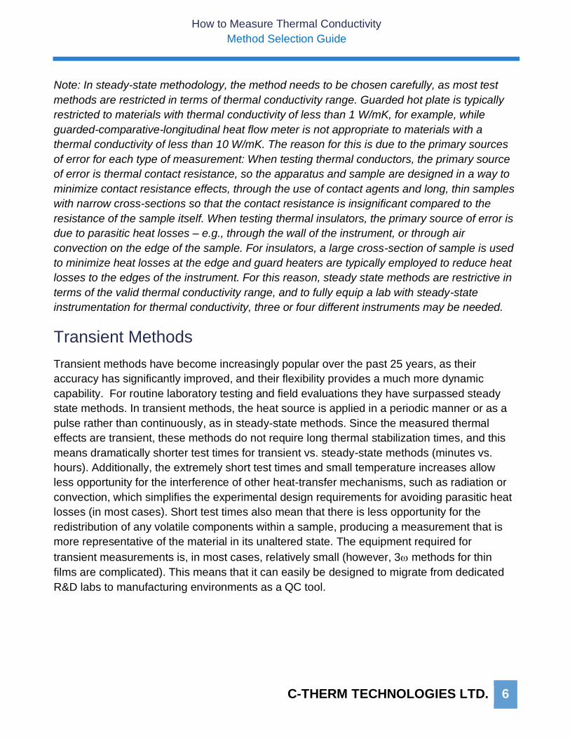
Transient Methods
Transient methods have become increasingly popular over the past 25 years, as their
accuracy has significantly improved, and their flexibility provides a much more dynamic
capability. For routine laboratory testing and field evaluations they have surpassed steady
state methods. In transient methods, the heat source is applied in a periodic manner or as a
pulse rather than continuously, as in steady-state methods. Since the measured thermal
effects are transient, these methods do not require long thermal stabilization times, and this
means dramatically shorter test times for transient vs. steady-state methods (minutes vs.
hours). Additionally, the extremely short test times and small temperature increases allow
less opportunity for the interference of other heat-transfer mechanisms, such as radiation or
convection, which simplifies the experimental design requirements for avoiding parasitic heat
losses (in most cases). Short test times also mean that there is less opportunity for the
redistribution of any volatile components within a sample, producing a measurement that is
more representative of the material in its unaltered state. The equipment required for
transient measurements is, in most cases, relatively small (however, 3 methods for thin
films are complicated). This means that it can easily be designed to migrate from dedicated
R&D labs to manufacturing environments as a QC tool.

How to Measure Thermal Conductivity
Method Selection Guide
C-THERM TECHNOLOGIES LTD. 7
Innovations in Thermal Conductivity Testing – An
Overview of Transient Methods
C-Therm has pioneered the advancement of transient methods, building a reputation for
world class thermal conductivity instruments. The C-Therm Trident Thermal Conductivity
Instrument represents a new paradigm in measurement of the heat transfer property by
delivering three of the most powerful transient methods in one instrument. It’s better to have
options.
Trident offers the precision of MTPS (modified transient plane source method), the flexibility
of TPS (transient plane source method), and the robustness of TLS (transient line source
needle method), all in one modular package (Figure 1). These options support a wide range
of applications without sacrificing ease of use.
Figure 1. C-Therm Trident Thermal Conductivity Instrument.

How to Measure Thermal Conductivity
Method Selection Guide
C-THERM TECHNOLOGIES LTD. 8
MTPS: Modified Transient Plane Source Method
The Modified Transient Plane Source (MTPS) Method (ASTM D7984-16) is an enhancement
of the Transient Plane Source Method that requires only a single-sided interface with the
sample during the measurement of thermal properties. It employs a one-sided interfacial
heater/sensor (Figure 2) surrounded by an integrated heated guard ring. The patented
heater/sensor applies a transient heat pulse to the sample, as shown in Figure 3 below. The
heated guard ring provides a thermal barrier that surrounds the heater/sensor and eliminates
lateral heat transfer at the sensor/sample interface. The heater/sensor/guard ring assembly
resides on a base of low thermal effusivity to ensure that nearly all the heat transferred in a
measurement occurs between the heater/sensor/guard ring and the sample.
In operation, the heater/sensor/guard ring assembly is placed in intimate contact with a
sample, as illustrated in Figure 3 above. To ensure reproducibility in the contact between the
sample and the heater/sensor and to minimize thermal contact resistance, a specific weight is
typically placed on the sample. A momentary electrical current is simultaneously applied to
both the spiral heater/sensor and the guard ring. The presence of an electrically heated guard
Figure 3. C-Therm MTPS Thermal Conductivity Sensor showing sensor assembly and specimen mounting.
Figure 2. A Modified Transient Plane Source Thermal Conductivity sensor.

How to Measure Thermal Conductivity
Method Selection Guide
C-THERM TECHNOLOGIES LTD. 9
ring ensures that heat transfer between the heater/sensor spiral and the sample
approximates one-dimensional heat flow. This specific incorporation of the guard ring in the
design of the sensor is a significant innovation C-Therm developed for single-sided testing.
No other vendor offers the patented guard ring technology.
The sensor temperature is factory calibrated using the relationship:
𝑅(𝑇) = 𝑅0 + 𝐴 ∙ 𝑇 (17)
and R(T) is the resistance of the sensor at a given temperature, R0 is the resistance of the
sensor at 0C, T is the temperature and A is the slope of the graph of resistance vs.
temperature. The slope is equal to:
𝐴 = 𝑅0 ∙ 𝑇𝐶𝑅 (18)
where TCR is the temperature coefficient of resistance of the sensor. TCR is constant over
the measured temperature range and the sensor is calibrated to determine the TCR within
this range. Once the MTPS sensor has undergone TCR calibration, the instantaneous
surface temperature of the sensor is then:
𝑇 =𝑅(𝑇)−𝑅0
𝐴 (19)
The MTPS measures the sensor resistance directly:
𝑅 =𝑉0
𝐼 (20)
or calculates it from the initial voltage, V0 or power:
𝑅 =𝑉0
2
𝑃 (21)
When in contact with sample material, the short current pulse is applied to the heater/sensor
to raise its temperature by 1 to 3C. The rate at which the temperature at the heater/sample
interface climbs during the current pulse is proportional to both the input power and the
thermal losses due to conduction away from the interface by the sensor substrate and the
sample.
Knowledge of the instantaneous temperature of the sensor allows the determination of the
thermal characteristics of a material in contact with the sensor. The heat equation for the
sensor in contact with the sample and with a constant supply of heat per second per volume,
G’, is given by:

How to Measure Thermal Conductivity
Method Selection Guide
C-THERM TECHNOLOGIES LTD. 10
𝜌𝐶𝑝𝜕𝑇
𝜕𝑡= 𝜅
𝜕2𝑇
𝜕𝑥2 + 𝐺′ (22)
Assuming that two semi-infinite media are in contact with the heat generated at the interface
and that one medium is represented by the effusivity, e1, of the sensor and that the other, e2,
is the tested sample material (Figure 4).
Then, when temperature of both media at the interface is identical and in thermal equilibrium
after contact has been established, the solutions to (31) for the sensor and sample are:
(Sensor) Δ𝑇1(𝑥, 𝑡) =2𝐺√𝑡
𝑒1+𝑒2𝑖𝑒𝑟𝑓𝑐
|𝑥|
2√𝑎1∙𝑡 𝑓𝑜𝑟 𝑥 < 0, 𝑡 > 0 (23)
(Sample) Δ𝑇2(𝑥, 𝑡) =2𝐺√𝑡
𝑒1+𝑒2𝑖𝑒𝑟𝑓𝑐
|𝑥|
2√𝑎2∙𝑡 𝑓𝑜𝑟 𝑥 ≥ 0, 𝑡 > 0 (24)
where: T = the change in sensor surface temperature (C);
G = the power flux supplied to the sensor (W/m2);
t = time measured from the start of the process (sec);
e1 = equivalent effusivity of the sensor (= √𝜅1 ∙ 𝐶𝑝1 ∙ 𝜌1 ,𝑊√𝑠
𝑚2𝐾);
e2 = effusivity of the sample material (= √𝜅2 ∙ 𝐶𝑝2 ∙ 𝜌2 ,𝑊√𝑠
𝑚2𝐾);
a1 = equivalent diffusivity of the sensor, m2/s;
a2 = diffusivity of the sample material, m2/s;
1 = equivalent thermal conductivity of the sensor, W/mK;
2 = thermal conductivity of the sample material, W/mK;
1 = equivalent density of the sensor, kg/m3;
x = 0
The interface
between the
sensor and the
sample
x < 0
e1
Sensor
x ≥ 0
e2
Sample
Sen
sor
Sam
ple
Figure 4.

How to Measure Thermal Conductivity
Method Selection Guide
C-THERM TECHNOLOGIES LTD. 11
2 = density of the sample material, kg/m3;
Cp1 = equivalent heat capacity of the sensor, J/kgK;
Cp2 = heat capacity of the sample material, J/kgK;
ierfc = integral of the error function
If no thermal contact resistance exists at the interface between the sensor and the sample,
then T1(x=0, t) = T2(x=0, t) at all points having x=0 and Equations (23) and (24) become:
ΔT(𝑥 = 0, 𝑡) =2𝐺√𝑡
𝑒1+𝑒2∙ 0.5642 =
1.1284𝐺√𝑡
𝑒1+𝑒2 (25)
From Equation (17), the change in resistance of the sensor at time, t, is:
∆𝑅(𝑡) = 𝑅(𝑡) − 𝑅(𝑡 = 0) = 𝐴 ∙ ∆𝑇(𝑥 = 0, 𝑡) (26)
And, from V=IR and Equation (26), the voltage change at time, t, is:
∆𝑉(𝑡) = 𝐼 ∙ ∆𝑅(𝑡) = 𝐼 ∙ 𝐴 ∙ ∆𝑇(𝑥 = 0, 𝑡)
= 𝑚√𝑡 =1.1284𝐼∙𝐴∙𝐺√𝑡
𝑒1+𝑒2 (27)
where 𝑚 =1.1284𝐼∙𝐴∙𝐺
𝑒1+𝑒2.
Figure 5 shows a plot of voltage change vs. the square root of time. Once the system has
stabilized, the graph shows a linear response with slope m. The inverse of the slope, m, can
be written:
1
𝑚=
𝑒1+𝑒2
1.1284𝐼∙𝐴∙𝐺=
𝑒1
1.1284𝐼∙𝐴∙𝐺+
𝑒2
1.1284𝐼∙𝐴∙𝐺 (28)

How to Measure Thermal Conductivity
Method Selection Guide
C-THERM TECHNOLOGIES LTD. 12
If we consider a measurement in which the “sample” is a vacuum, then e2 is the effusivity of
vacuum, e2 = 0, and Equation (28) reduces to:
1
𝑚(𝑣𝑎𝑐𝑢𝑢𝑚) =
𝑒1
1.1284𝐼∙𝐴∙𝐺 (29)
Values of the voltage/time slope, m, for a series of calibration materials with known
effusivities can be determined experimentally using the MTPS sensor and a plot of 1/m for
these materials is linear as shown in Figure6.
The slope of the effusivity calibration curve is M and the equation of the calibration line is:
1
𝑚= 𝑀 × 𝑒2 + 𝐶 (30)
where e2 is the effusivity of the sample, C is the 1/m value of the sensor for vacuum, and the
slope M is equal to:
𝑀 =1
1.1284𝐼∙𝐴∙𝐺 (31)
Figure 5. MTPS sensor voltage response vs. the square root of
time.
Figure 6. 1/m sensor effusivity calibration curve.

How to Measure Thermal Conductivity
Method Selection Guide
C-THERM TECHNOLOGIES LTD. 13
Since:
𝐶 = 𝑖𝑛𝑡𝑒𝑟𝑐𝑒𝑝𝑡 =1
𝑚(𝑣𝑎𝑐𝑢𝑢𝑚) =
𝑒1
1.1284𝐼∙𝐴∙𝐺 (32)
then the equivalent effusivity of the sensor, e1, is given by:
𝐶
𝑀=(
𝑒1
1.1284𝐼∙𝐴∙𝐺) × (
1.1284𝐼∙𝐴∙𝐺
1) = 𝑒1 (33)
Thus, the effusivity calibration curve allows the determination of effusivity values for both the
sensor and the sample. Knowledge of the slope of the voltage vs sqrt (time) response of the
MTPS sensor provides 1/m values for unknown samples. So long as those 1/m value of the
unknown material lies within the range of the 1/m calibration curve determined using
calibration materials of known effusivity, the effusivity of the unknown sample, e2, can be
determined from the graph in Figure6 and Equation (30).
Two methods may be used to determine the thermal conductivity of a test sample. When the
density, , and specific heat, Cp, of the test sample are known, the thermal conductivity, ,
can be calculated using the effusivity, determined as described above, and the relationship:
𝜅 =𝜀2
2
𝜌∙𝐶𝑝 (34)
More commonly the density and specific heat of the sample are unknown, and the thermal
conductivity is determined using a graphical method similar to that used for the determination
of effusivity. The same 1/m data determined for the measurement of sample effusivity is used
as input to a unique algorithm (the m* algorithmvii) that employs an iterative process and the
thermal conductivity of known materials to create a sensor calibration curve for thermal
conductivity. The thermal conductivity calibration relationship has the form:
1
𝑚−𝑚∗= 𝑆𝑙𝑜𝑝𝑒 ∙ 𝑘 + 𝐼𝑛𝑡𝑒𝑟𝑐𝑒𝑝𝑡 (35)

How to Measure Thermal Conductivity
Method Selection Guide
C-THERM TECHNOLOGIES LTD. 14
𝜅 = [1
𝑚−𝑚∗−𝐼𝑛𝑡𝑒𝑟𝑐𝑒𝑝𝑡
𝑆𝑙𝑜𝑝𝑒] (36)
where: m is the value of the slope determined for the voltage vs. √𝑡𝑖𝑚𝑒 curve of the sample,
shown in Figure 5, “Slope” is the slope and “Intercept” is the intercept of the 1
(𝑚−𝑚∗) vs.
thermal conductivity calibration curve shown in Figure7, and m* is a calibration factor that
linearizes the measured 1/m with the known conductivities of the calibration materials as
shown in Figure7.
In the procedure for thermal conductivity calibration, values for m are determined for a series
of calibration standards of known thermal conductivity that bracket the expected value of the
test sample. The values for m and thermal conductivity of the calibration standards are then
used as input to an iterative linear regression to solve Equation (36). m* is treated as a
variable fitting parameter during the regression with the value iteratively adjusted to provide
the best least squares fit of the relationship to the data.
Maintaining high accuracy and precision across a broad range of thermal conductivity and
effusivity using the MTPS technique requires that the sensor calibration is sub-divided into
ranges that bracket the expected sample value, and the power and timing parameters must
be optimized for a given group of materials. For example, longer test time and lower power
settings are optimal for achieving a deeper depth of penetration when measuring insulation
materials like foams. Conversely, shorter test time and higher power settings are optimal for
higher-conductivity metals where the pulse travels very quickly through the material and a
shorter test time provides for more flexibility in limiting the thickness requirements of the
sample. Each group of materials has its calibration curve.
Figure 7. MTPS thermal effusivity and conductivity calibration plots.

How to Measure Thermal Conductivity
Method Selection Guide
C-THERM TECHNOLOGIES LTD. 15
One thing to note is that the above discussion illustrates the theory of operation of the
Modified Transient Plane Source method. However, on the user experience side, all MTPS
sensors are factory calibrated. No user calibration is required, and the sensors are ‘plug and
play’. The MTPS sensor can measure thermal conductivity of materials in seconds, fast and
easy to use. The user interface provides a tabular output of thermal conductivity, effusivity
and temperature. The factory-provided calibration results in the easiest method for a user to
obtain accurate and consistent thermal conductivity data.
MTPS Key Applications:
MTPS Application Highlight: Evaluating Thermal Performance of Advanced Materials
Thermal energy management is an important design criterion when designing new buildings
and renovating existing structures. Recently, thermal energy storage within these building
materials used in a structure has been gaining increasing interest and many new candidate
materials are being evaluated for this purpose. One class of materials that have
demonstrated promising characteristics in this application is phase change materials (PCMs).
PCMs store latent heat energy not only as sensible heat in the thermal mass of the material
but also in the latent heat associated with phase changes. This means that significantly less
material is required to sequester thermal energy for heating and cooling the structure.
One recent study by Lee et alviii provides a good representative example of the use of the
MTPS method in quantifying the thermal energy storage characteristics of new materials.
This study examined the thermal storage behavior of shape-stabilized PCMs (SSPCMs) of
exfoliated graphite nanoplatelets (xGnP) impregnated with fatty acid ester coconut oil and

How to Measure Thermal Conductivity
Method Selection Guide
C-THERM TECHNOLOGIES LTD. 16
paraffin n-hexadecane. Fatty acid esters such as coconut oil are readily available, natural
PCMs that are relatively inexpensive. Paraffins such as n-hexadecane are desirable in these
applications owing to their large latent heat capacity and stability. However, both materials
suffer from the fact that they have inherently low thermal conductivities and dimensional
stability which makes them unsuitable for use as structural PCMs. These problems can be
potentially resolved by incorporating the ester and paraffin materials into a stable material
matrix that has acceptable thermal conductivity. xGnP provides such a substrate. xGnPs are
porous, nanostructured substrate materials with high thermal conductivities that can absorb
relatively large quantities of organic PCM substances. If the thermal conductivity of
xGnP/coconut oil/n-hexadecane SSPCMs can be shown to retain high thermal conductivity, it
provides a key qualification for their use as structural thermal storage materials.
Lee’s study prepared samples of xGnPs infused with different amounts of coconut oil and n-
hexadecane using a vacuum impregnation process that ensured good penetration of the
PCM material into the layered, porous structure of the xGnP. xGnP test samples were loaded
with 70/30, 50/50, and 30/70 mixtures of coconut oil/n-hexadecane. The samples were
analyzed using electron microscopy (SEM), infrared spectroscopy (FTIR), differential
scanning calorimetry (DSC), thermogravimetric analysis (TGA), and MTPS thermal
conductivity analysis. SEM analyses of the impregnated xGnP samples containing different
loadings of PCM confirmed the saturation by the PCMs and that the impregnation process
caused no significant change in the xGnP structure. FTIR analyses confirmed that the
coconut oil and n-hexadecane were stable on absorption by the xGnP samples, with no
indication of chemical changes apparent in the spectra. Individual peak intensities in the
sample spectra were consistent with the different relative loadings of coconut oil and n-
hexadecane. These analyses showed that the physical and chemical nature of the substrate
and PCMs did not undergo significant change when the SSPCM was formed, a necessary
qualification for use in structural thermal storage applications.
DSC analyses showed that the SSPCMs containing a 30/70 mixture of coconut oil/n-
hexadecane exhibited a 30 percent increase in latent heat capacity over xGnPs with similar
loadings of either of the PCMs alone. TGA analyses showed all mixtures of coconut oil/n-
hexadecane in nGnP substrates to be thermally stable at the temperatures that might be
encountered in structural thermal storage applications.

How to Measure Thermal Conductivity
Method Selection Guide
C-THERM TECHNOLOGIES LTD. 17
The thermal conductivity analysis used C-Therm’s MTPS method (sensor) to determine
thermal conductivities for all xGnP/coconut oil/n-hexadecane samples. The MTPS sensor
was preferred for this study owing to the small sample requirements and the fact that it was
necessary to determine the thermal conductivity of materials having physical properties that
made them unsuitable for measurement using the TPS or TLS methods. The thermal
conductivities of pure coconut oil and n-hexadecane were also determined using the MTPS
method. Pure coconut oil had a thermal conductivity of 0.321 W/mK and pure n-hexadecane
had a thermal conductivity of 0.154 W/mK. All tests were performed at 10C and the results
are shown in Figure 8. The thermal conductivity analyses using MTPS showed that
impregnating xGnP with mixtures of coconut oil and n-hexadecane produced an SSPCM with
thermal conductivity much superior to that of either coconut oil or n-hexadecane alone.
Comparison of xGnP containing different mixture ratios of coconut oil to n-hexadecane
showed that those with greater coconut oil concentrations had the highest thermal
conductivity.
This study shows how the MTPS method, along with other physical, chemical and
characterization tools, can provide data for the physical and thermal properties of advanced
structural materials. This data is required as a design tool for the energy-efficient buildings
that must be developed for a future that supports sustainable living.
Figure 8. Thermal conductivities of mixed SSPCMs.

How to Measure Thermal Conductivity
Method Selection Guide
C-THERM TECHNOLOGIES LTD. 18
TPS: Transient Plane Source Method
The Transient Plane Source Method (TPS), ISO 22007-2,ix uses a heated disc composed of a
bifilar nickel spiral (contains two closely spaced spiral windings) encapsulated in a dielectric
material such as Kapton® (Figure 10). During a measurement, the sensor is positioned
between two identical samples of the material being measured as shown; a pulse of constant
electrical power (up to minutes in duration) is applied to the spiral heater and the increase in
temperature in the spiral is measured. The spiral in the sensor serves as both the source of
heat and a dynamic temperature sensor during a measurement. The sensor and bridge
circuitry is shown in Figure 10, including the DC power supply, V standard resistance, Re,s,
and measurement points for the sensor voltage drop (V2) and the voltage drop across the
standard resistor (V1).
The sensor temperature response is factory calibrated using the temperature coefficient of
resistance, TCR, of the nickel spiral. TCR relates to the change in metal resistance with a
change in temperature. The use of this relationship, as employed in this application is
described in ISO Standard 22007-2x and TCR is defined in the British Standards Institute’s
BS EN 60751 Standardxi. BS EN 60751 defines a quadratic or cubic model for the
Figure 10. Left: The TPS probe configuration showing bridge circuit, contacts and
bifilar spiral sensor; Right: Sensor positioning between sample pieces [19].
Figure 9. A Transient Plane Source sensor.

How to Measure Thermal Conductivity
Method Selection Guide
C-THERM TECHNOLOGIES LTD. 19
temperature-resistance characteristics of a metal. For example, in the case of a platinum
resistor, the temperature-resistance characteristic has the following form:
𝑅(𝑇) = 𝑅0[1 + 𝐴 ∙ 𝑇 + 𝐵𝑇2] for 0 < T < 850C (3)
𝑅𝑇 = 𝑅0[1 + 𝐴𝑇 + 𝐵𝑇2 + 𝐶(𝑇 − 100)𝑇3] for -200 < T < 0C (4)
Where R(T) is the resistance of the metal at a given temperature, R0 is the resistance of
metal at 0C, T is the temperature, and A, B, and C are constants.
The current and time of the electrical pulse are calibrated to cause an expected temperature
rise of one to several degrees in the sensor, based on the power delivered and the known
TCR of the nickel spiral. As the temperature rises in the sensor, there is a corresponding
increase in its resistance, and this produces a measurable change in the voltage drop over
the sensor. To retain accuracy in the operational model of the TPS measurement, the
duration of the measurement must be short for the thermal diffusivity of the sample. This
allows the approximation that the sensor can be considered as being in contact with an
infinite solid. Under this assumption, the sensor temperature is influenced only by the power
input and the thermal transport properties of the solid in contact with the sensor, and not by
any boundary effects.
The behavior of the TPS sensor during the transient pulse can be understood in terms of its
time-dependent resistance, described by the equation (for small increases in temperature
∆𝑇):
𝑅(𝑡) = 𝑅0[1 + 𝑎∆𝑇(𝑡)̅̅ ̅̅ ̅̅ ̅̅ ] (5)
where R(t) is the time-dependent resistance, R0 the initial resistance of the TPS element
before the transient pulse, the TCR of the sensor element, and ∆𝑇(𝑡)̅̅ ̅̅ ̅̅ ̅̅ is the mean value of the
time-dependent temperature increase in the TPS sensor element. The temperature increase
is dependent on the supplied power, the geometry of the sensor and the properties of the
sample. It can also be expressed as ∆𝑇(𝜏) where the variable is a non-dimensional
characteristic time parameter and is defined as:
𝜏 = (𝑡𝜃⁄ )
12⁄
, 𝜃 = 𝑟2
𝛼⁄ (6)
Where t is the time as measured from the start of the transient pulse, r the radius of the
sensor spiral (largest ring) and is the thermal diffusivity of the sample material.
In the case of a spiral sensor element (other geometries are possible), the time-dependent
temperature increase of the sensor (Figure 11) is given by:

How to Measure Thermal Conductivity
Method Selection Guide
C-THERM TECHNOLOGIES LTD. 20
∆𝑇(𝜏)̅̅ ̅̅ ̅̅ ̅̅ =𝑃
𝜋3 2⁄ 𝑟𝜅𝐷(𝜏) (7)
Where ∆𝑇(𝜏)̅̅ ̅̅ ̅̅ ̅̅ is the mean temperature rise of the sensor, P is the input power to the sensor, r
is the sensor radius, is the thermal conductivity of the sample, and D() is a shape function
specific to the sensor geometry and depends on the thermal diffusivity of the sample α. The
mean temperature the function can be modified to take into account the thermal resistance
between the sample and the sensor:
∆𝑇(𝜏) = 𝐴 +𝑃
𝜋3 2⁄ 𝑟𝜅𝐷 [(
𝛼(𝑡−𝑡𝑐)
𝑟2 )1/2
] (8)
where A is the temperature drop on the total thermal resistance between the sensor and the
sample, 𝛼 is the thermal diffusivity and it is a time correction that takes into account thermal
inertia of the sensor and various delays in the electronics of the apparatus. Equation (8) is
true if and only if the thermal resistances on both sides of the sensor are equal, resulting in
steady and equal heat flux to each side.
The TPS method can be applied in different measurement modes. These are Isotropic Bulk
Mode, Anisotropic Bulk Mode, and Slab Mode. In all measurement modes, the setup must be
symmetrical on both sides of the sensor.
TPS Isotropic and Anisotropic Bulk Measurement Mode: In the Isotropic Bulk Mode, the
sensor is in contact with two identical isotropic samples such that their size in all directions is
larger than the penetration depth of the heatwave over the entire measurement time. A bulk
sample thus approximates an “infinite” sample size. The shape function for the isotropic bulk
mode, D(), models the sensor as concentric ring sources and has the form:
𝐷(𝜏) =1
𝑛2(𝑛+1)2 × ∫𝑑𝑠
𝑠2∑ 𝑙 ∑ 𝑘 𝑒𝑥𝑝 (−
𝑙2+𝑘2
4𝑛2𝑠2) 𝐼0 (𝑙𝑘
2𝑛2𝑠2)𝑛𝑘=1
𝑛𝑙=1
𝜏
0 (9)
Figure 11. A typical temperature rise vs. time curve for a TPS
measurement.

How to Measure Thermal Conductivity
Method Selection Guide
C-THERM TECHNOLOGIES LTD. 21
where n is the number of concentric rings, I0 the modified Bessel function of the zeroth order
and s is the integration variable, l and k are summation variables. In practice, Equations (5)
and (6) are combined and the resulting equation is used, along with temperature
measurements over a suitable time window. A data fitting procedure such as least squares
regression is used that allows the determination of both the thermal diffusivity, α, and the
thermal conductivity of the sample, .
The anisotropic bulk mode is limited to orthotropic samples, i.e. samples in which thermal
transport properties are identical in all directions parallel to sensor surface but have different
values vertical to the sensor surface. In this case, Equation (7) becomes
∆𝑇(𝜏)̅̅ ̅̅ ̅̅ ̅̅ =𝑃
𝜋32∙𝑟√𝜅𝑟𝜅𝑧
𝐷(𝜏) (10)
where 𝜅𝑟 is the thermal conductivity parallel to the sensor surface and 𝜅𝑧 is the thermal
conductivity orthogonal to the sensor surface, and 𝐷(𝜏) is calculated with the thermal
diffusivity in parallel to the sensor surface, 𝛼𝑟. Instead of Equation (6), Equation (11) is used
for 𝜃 and 𝜏.
𝜏 = (𝑡𝜃⁄ )
12⁄
, 𝜃 = 𝑟2
𝛼𝑟⁄ (11)
It is important to be aware of the assumptions inherent in the TPS method. It assumes that
the sample provides an infinite medium for thermal transfer. In practical terms, this means
that, ideally, a sample needs to be 2-3 times the sensor diameter in width and length and at
least the sample diameter in thickness. The model treats the spiral sensor as concentric
rings, an approximation that imposes some error in the measurement which increases as r
decreases. The method assumes a complete symmetry on both sides of the sensor, meaning
that the sensor insulation layers on both sides are identical and that any parasitic thermal
contact resistance must be identical on both sides. While this condition may never be
completely valid, applying a clamping force or weight on the sensor-sample system
minimizes the resulting error. As well, the assumption that a sample’s thermal properties
don’t change during measurement imposes a limit on how large of a temperature increase
may be applied to the sample. These issues impose certain restrictions on the method:
• The method cannot be performed in an asymmetric sampling configuration since
contact resistance affects the shape factor and the mathematical model has not yet
been expanded to include contact resistance;
• Care must be taken in setup to ensure contact resistance is equal on both sides. This
requires:
o High pressure applied to both sides of the sample;

How to Measure Thermal Conductivity
Method Selection Guide
C-THERM TECHNOLOGIES LTD. 22
o Careful preparation of a smooth sample surface
▪ Very small surface imperfections, if not symmetrical, can introduce very
large errors into the measurement.
o Identical samples for multiple measurements
• Samples must be large enough to accommodate a valid test time. Practically, this
means sample restrictions as follows:
o Diameter: >5r, where r is the sensor radius
o Thickness: >2r, where r is the sensor radius
• Test time must be chosen to be long enough that deviations from circular geometry do
not affect the validity of the test result, but short enough that thermal diffusion effects
are still significant in the shape factor
o The test result is valid if the following inequality is satisfied:
1.1𝑟 ≤ √4𝛼𝑡 ≤ 2.0𝑟
Where:
• r is sensor radius
• 𝛼 is thermal diffusivity
• 𝑡 is the maximum analysis time boundary
TPS Isotropic Slab Measurement Mode: The Isotropic Slab Mode is used when the
approximation of an "infinite" sample size is no longer valid due to a restriction in the
thickness of the sample. In this mode, thin sample slabs, or plates, can be used. The size of
the samples must be adequately large ("infinite") in the directions parallel to the sensor
surface, but relatively thin normal to the sensor surface. The external slab surfaces must be
adequately insulated against heat loss, or alternatively, the measurement should be
conducted in a vacuum. For high thermal diffusivity materials, this is the preferred method as
it improves signal strength and decreases the sample size. As in the bulk mode, two identical
samples are used.
In the Isotropic Slab Measurement Mode Equation (6) holds, but the shape function, 𝐸(𝜏)
becomes:
How to Measure Thermal Conductivity
Method Selection Guide
C-THERM TECHNOLOGIES LTD. 23
𝐸(𝜏) = [𝑛(𝑛 + 1)]−2 × ∫ 𝑠−2 [∑ 𝑙 ∑ 𝑘 𝑒𝑥𝑝 (−(𝑙2+𝑘2)
4𝑛2𝑠2 )𝑛𝑘=1
𝑛𝑙=1 𝐼0 (
𝑙𝑘
2𝑛2𝑠2)] {1 + 2 ∑ 𝑒𝑥𝑝 [𝑖2
𝑠2 (ℎ
𝑟)
2]∞
𝑖=1 } 𝑑𝑠𝜏
0
(12)
where n is the number of concentric rings, r is the sensor radius, h is the thickness of the two
slabs, and s is the integration variable. One assumption made in deriving this function is that
the material is isotropic – therefore this method cannot be used in measuring anisotropic
materials.
Since thermal conductivities are obtained by fitting experimental data to the theoretical
operating equations of the TPS method, the primary limitation of this method is that it is
heavily dependent on the user's expertise and intuition for accurate results. This makes the
technique prone to operator bias. The user must establish appropriate timing and power
parameters and select sensors appropriate for specific types of measurements based on the
expected thermal conductivity of the material. Lack of knowledge of the range of possible
values for a sample’s thermal conductivity requires multiple tests and can produce confusing
results.
Limitations on test time, symmetry of test assembly, contact resistance, and sample diameter
are identical for this method as for the bulk method. Thickness may be between 1mm and the
lesser of the sensor radius or 10 mm.
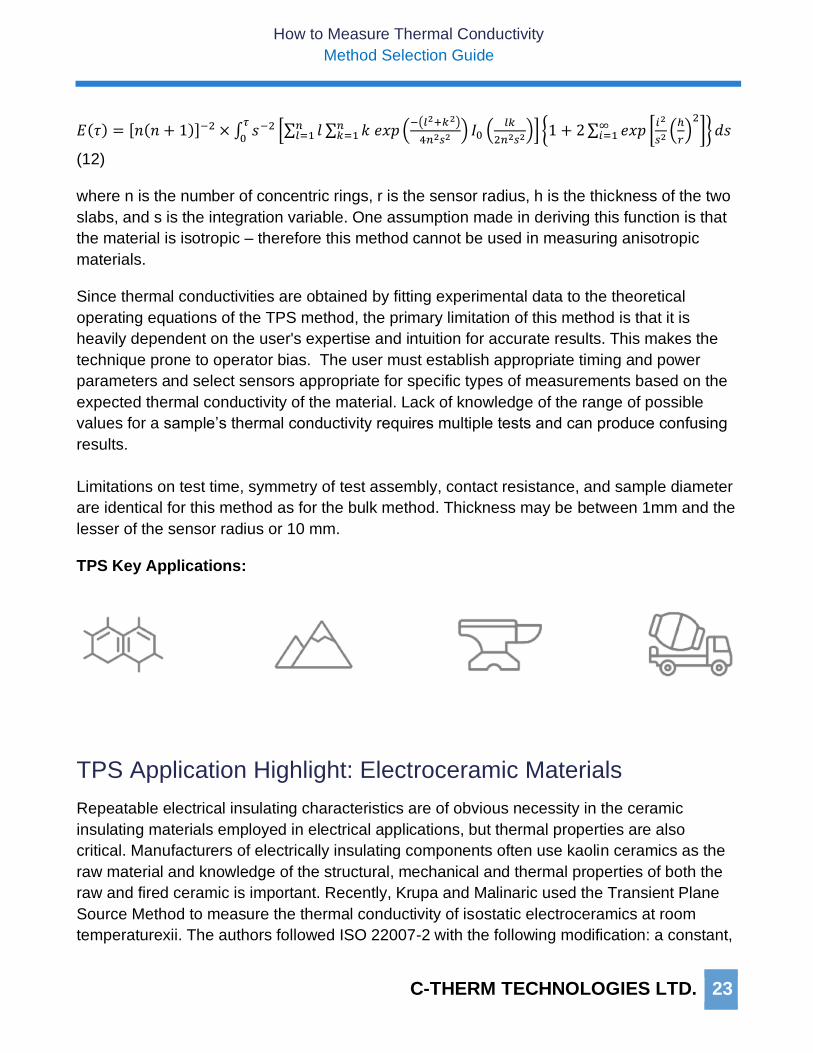
TPS Key Applications:
TPS Application Highlight: Electroceramic Materials
Repeatable electrical insulating characteristics are of obvious necessity in the ceramic
insulating materials employed in electrical applications, but thermal properties are also
critical. Manufacturers of electrically insulating components often use kaolin ceramics as the
raw material and knowledge of the structural, mechanical and thermal properties of both the
raw and fired ceramic is important. Recently, Krupa and Malinaric used the Transient Plane
Source Method to measure the thermal conductivity of isostatic electroceramics at room
temperaturexii. The authors followed ISO 22007-2 with the following modification: a constant,

How to Measure Thermal Conductivity
Method Selection Guide
C-THERM TECHNOLOGIES LTD. 24
A, was added to account for contact resistance between the sensor and sample. Provided the
contact resistances on both sides of the sensor are identical, this does not affect the analysis.
The samples used in the study were made from weighed mixtures of the raw material that
contained a precise ratio of clay, kaolin, feldspar, aluminum oxide, quartz and other materials
that had been ball-milled to a fine powder. The dry mixture was isostatically compacted in a
die-press and coupons were cut from the “green body” and precision-machined to a
reproducible shape for firing. The samples were then fired at different temperatures using
tightly controlled heating/cooling rates. Depending on the material mixture and firing
conditions, different reactions, ranging from simple de-hydroxylation to chemical
recombination were possible, producing fired samples with a variety of thermal, physical,
chemical and electrical properties.
The authors used a 6.4 mm diameter sensor with 16 circular rings in a conventional TPS
sampling configuration to evaluate the thermal conductivity of the fired sample coupons. They
used a modified electrical bridge circuit that suppressed voltage source instability and
removed the resistance of the sensor leads from the calculations. The authors employed the
modified mean temperature function:
𝑇(𝑡)̅̅ ̅̅ ̅̅ = 𝐴 +𝑃
𝜋3
2⁄ 𝑟𝜆𝐷 [(
𝛼(𝑡 − 𝑡𝑐)
𝑟2)
12
] (𝟏𝟑)
in which A corresponds to the temperature drop on the total thermal resistance between the
sensor heater and the samples (i.e. including the sensor insulation layers) and time
correction, etc, accommodates thermal inertia in the sensor and delays in the electronics.
How to Measure Thermal Conductivity
Method Selection Guide
C-THERM TECHNOLOGIES LTD. 25
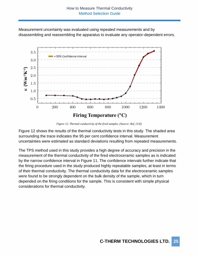
Measurement uncertainty was evaluated using repeated measurements and by
disassembling and reassembling the apparatus to evaluate any operator-dependent errors.
Figure 12 shows the results of the thermal conductivity tests in this study. The shaded area
surrounding the trace indicates the 95 per cent confidence interval. Measurement
uncertainties were estimated as standard deviations resulting from repeated measurements.
The TPS method used in this study provides a high degree of accuracy and precision in the
measurement of the thermal conductivity of the fired electroceramic samples as is indicated
by the narrow confidence interval in Figure 11. The confidence intervals further indicate that
the firing procedure used in the study produced highly repeatable samples, at least in terms
of their thermal conductivity. The thermal conductivity data for the electroceramic samples
were found to be strongly dependent on the bulk density of the sample, which in turn
depended on the firing conditions for the sample. This is consistent with simple physical
considerations for thermal conductivity.
Figure 12. Thermal conductivity of the fired samples. (Source: Ref. [14])

How to Measure Thermal Conductivity
Method Selection Guide
C-THERM TECHNOLOGIES LTD. 26
TLS: Transient Line Source Method
The Transient Line Source Method (ASTM D5334, D5930, and IEEE Std 442-1981) uses a
needle probe such as the one shown in Figure 23. During a measurement, the needle is
inserted into a sample material such as a soft soil (ASTM D5334), plastic (D5930), or liquid
that is at a uniform and constant initial temperature. A typical needle probe consists of a 150
mm long stainless-steel hypodermic tube as shown in Figure3xiii. Within the tube are the line
heating source that provides a known amount of heat during the measurement and two
thermocouple junctions positioned to measure the transient temperature rise (T1) and
reference temperatures (T2) when the transient heat pulse is applied. In operation, a known
amount of heat energy in the form of a heat pulse is applied to the line heating source
(proportional to the known power supplied during the pulse) and this produces a heatwave
that propagates radially away from the needle probe and into the sample. The thermocouple
junction at T1 measures the rate of increase of the temperature in the middle of the heating
zone (Figure4) and this is used to calculate the thermal conductivity of the sample.
Figure 23. A Transient Line Source Probe.

How to Measure Thermal Conductivity
Method Selection Guide
C-THERM TECHNOLOGIES LTD. 27
The temperature rise in the line source varies linearly with the logarithm of time as shown in
Figure 35. The initial, non-linear portion of the curve in Figure 35, is due to heatwave
propagation through the walls of the tube and to thermal contact resistance when it is
present. The relationship between the rate of temperature rise and time in the linear region
can be used to calculate the thermal conductivity of the sample using the relationship:
𝜅 =𝐶𝑄
4𝜋∙𝑆𝑙𝑜𝑝𝑒 (14)
where
𝑄 = 𝐻𝑒𝑎𝑡 𝑖𝑛𝑝𝑢𝑡 𝑝𝑒𝑟 𝑙𝑒𝑛𝑔𝑡ℎ 𝑜𝑓 𝑤𝑖𝑟𝑒 (𝑊 𝑚⁄ ) = 𝐼2 𝑅
𝐿=
𝑉𝐼
𝐿 (15)
(I = Current, R = Wire Resistance, V = Voltage and L = Length of the heated wire)
and
𝑆𝑙𝑜𝑝𝑒 = 𝑇2−𝑇1
ln(𝑡2
𝑡1⁄ )
𝐾 (16)
Figure 35. Transient Line Source Temperature vs. Time Response.
Figure 14. Typical needle probe components (Source: [15]).

How to Measure Thermal Conductivity
Method Selection Guide
C-THERM TECHNOLOGIES LTD. 28
where T2 and T1 are temperatures recorded at times t2 and t1, respectively, during the
measurement. C is a calibration factor, (𝐶 =𝜆𝑚𝑎𝑡𝑒𝑟𝑖𝑎𝑙
𝜆𝑚𝑒𝑎𝑠𝑢𝑟𝑒𝑑), determined by measurement of
standard reference material. 𝜆𝑚𝑎𝑡𝑒𝑟𝑖𝑎𝑙 is the known thermal conductivity of the reference
material and 𝜆𝑚𝑒𝑎𝑠𝑢𝑟𝑒𝑑 is the thermal conductivity of the same material as measured by the
method and apparatus being used.
As with TPS, it is important to maintain an awareness of the assumptions employed in TLS.
The following assumptions are made in TLS measurements:
1. Thermal contact resistance is negligible;
a. This is only valid when the sample is symmetrical about the sensor.
2. The probe acts as a line source, with negligible heat capacity;
a. The sample volume must be much greater than the probe volume. For example,
a 1mm diameter probe requires a 3cm sample diameter.
3. The probe does not significantly contribute to the heat-transfer of the system;
a. This is never valid; it is the reason that the system must be calibrated.
4. The sample is in thermal equilibrium before the start of measurement;
5. The probe (and heating wire inside) is exactly linear;
a. Deviations from linear geometry may severely affect the measurement
accuracy.
6. Heat transfer occurs only through conduction;
a. TLS is inappropriate for measuring non-viscous fluids and other samples where
convection or radiation may significantly contribute to the heat transfer.
7. The sample is isotropic;
a. TLS is not recommended for anisotropic samples.
8. Sample properties do not change during measurement;
a. e.g., samples such as moist soils can lose moisture during the measurement.
How to Measure Thermal Conductivity
Method Selection Guide
C-THERM TECHNOLOGIES LTD. 29
9. The sample is homogeneous;
10. The sample behaves as an infinite medium.
Fortunately, the T vs. t plot for TLS measurements indicates when certain of these
assumptions are invalid in a sample measurement (6, 8, sometimes 9 and 10). For this
reason, it is important in TLS measurements to carefully inspect the T vs. t plot.
TLS Key Applications:
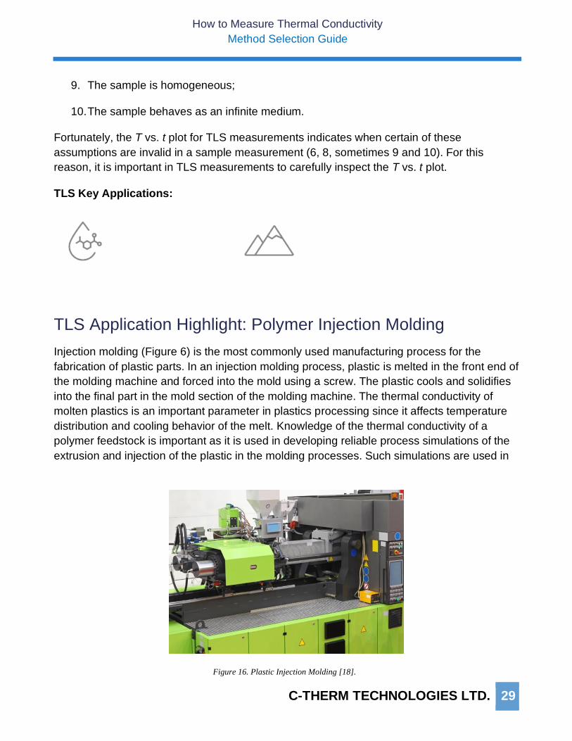
TLS Application Highlight: Polymer Injection Molding
Injection molding (Figure 6) is the most commonly used manufacturing process for the
fabrication of plastic parts. In an injection molding process, plastic is melted in the front end of
the molding machine and forced into the mold using a screw. The plastic cools and solidifies
into the final part in the mold section of the molding machine. The thermal conductivity of
molten plastics is an important parameter in plastics processing since it affects temperature
distribution and cooling behavior of the melt. Knowledge of the thermal conductivity of a
polymer feedstock is important as it is used in developing reliable process simulations of the
extrusion and injection of the plastic in the molding processes. Such simulations are used in
Figure 16. Plastic Injection Molding [18].
How to Measure Thermal Conductivity
Method Selection Guide
C-THERM TECHNOLOGIES LTD. 30
process control to achieve increased productivity and improved quality of the finished
product.
Injection molding process development begins with the prediction of a polymer’s melt
behavior under the conditions expected in the injection mold machine. These predictions are
accomplished using sophisticated rheological modelling that requires accurate knowledge of
the thermophysical properties of the polymer. The absolute value and variability of the
thermal conductivity of a polymer feedstock is a critical thermophysical parameter influencing
process performance in injection molding. The thermal conductivity of the polymer as it
passes through the transition from solid to melt and back dictates important process
parameters such as the heating rate and cooling time needed to avoid undesirable flaws such
as blistering, burn marks, warping or sink marks.
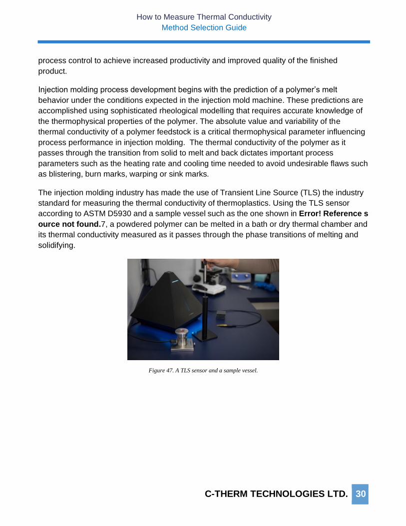
The injection molding industry has made the use of Transient Line Source (TLS) the industry
standard for measuring the thermal conductivity of thermoplastics. Using the TLS sensor
according to ASTM D5930 and a sample vessel such as the one shown in Error! Reference s
ource not found.7, a powdered polymer can be melted in a bath or dry thermal chamber and
its thermal conductivity measured as it passes through the phase transitions of melting and
solidifying.
Figure 47. A TLS sensor and a sample vessel.

How to Measure Thermal Conductivity
Method Selection Guide
C-THERM TECHNOLOGIES LTD. 31
A typical polymer thermal conductivity measurement using the TLS is shown in Figure 58.
The figure shows data for a sample of powdered polyamide 12 (Nylon-12), a thermoplastic
material commonly used in injection molding. The sample had thermal conductivity
measurements performed at 125°C, 150°C, and 200°C using a C-Therm Trident Thermal
Conductivity Analyzer equipped with a Transient Line Source (TLS) sensor. As this
application shows, C-Therm’s TLS sensor provides researchers and manufacturing engineers
in the polymer sector with a reliable, easy-to-use solution for measuring polymer melts.
Figure 58. Thermal Conductivity Test Results of Polyamide 12.

How to Measure Thermal Conductivity
Method Selection Guide
C-THERM TECHNOLOGIES LTD. 32
Putting Trident to Work
Trident reflects C-Therm’s years of experience working exclusively to provide labs,
researchers and manufacturers, with the very best in thermal conductivity measurement.
Modified
Transient
Plane Source
Transient
Plane
Source
Transient
Line
Source
Sample Preparation None
Sample simple rests on
top of sensor. A few
drops of contact agent
may be required.
Moderate to
Significant
Samples (2) must be
homogeneous with
smoothed mating
surfaces that sandwich
the sensor.
None to Minimal
Ranges from no
preparation for simple
soil probes to
containment and
heating for molten
plastic samples.
Operator Training
Requirements
Minimal Significant Minimal to Moderate
Non-Destructive Yes No Sample Dependent
Method Development Minimal Significant Minimal to Moderate
Material Phases Solids, Liquids,
Powders, Pastes
Solids, Liquids Liquids, Powders,
Pastes, Gels, Slurries,
Melts
Testing Time Seconds Minutes Minutes
Thermal Conductivity
Range
0-500 W/mK 0-100W/mK 0.1-6 W/mK
Temperature Range -50 - 200°C (500°C) -100 - 700°C -50 - 185°C
The simplest and quickest methods to implement and use are MTPS and TLS. These
techniques require minimal to moderate sample preparation and operator training.
The MTPS method simply requires the operator to place the sample on the one-sided
heater/sensor, add the supplied weight and “press go” on the analyzer. Analytical results for
the sample are available within seconds of mounting it on the sensor. No sample preparation
is needed, and an operator can be trained in minutes.
Table 2. A comparison of the characteristics of the MTPS, TPS, and TLS thermophysical analytical methods.

How to Measure Thermal Conductivity
Method Selection Guide
C-THERM TECHNOLOGIES LTD. 33
The use of TLS requires somewhat more operator training since, for example, powder and
soil samples must be reproducibly packed into sample holders and the melting of samples for
melt studies requires that heating and cooling characteristics are reproducible. Samples for
TLS may also require some preparation to ensure reproducible and homogeneous samples.
These requirements result in somewhat longer cycle times for TLS analyses as compared
with MTPS.
The TPS method requires significantly more sample preparation and operator training than
either the TLS or MTPS. The need for perfectly flat sample surfaces to “sandwich” the sensor
adds to both operator training requirements and sample preparation time. TPS results can be
highly dependent on the instrument operator.
The MTPS and TLS methods are the most broadly applicable in terms of sample types. Both
methods can be easily configured to analyze liquids, powders and pastes. MTPS and TLS
methods are complementary in that the MTPS probe is easily used with monolithic solids that
are not readily probed by TLS, while TLS probes can conveniently determine dynamic
thermophysical data for the melting behavior of plastic materials. The TPS method is
generally more limited in the physical states that can be analyzed, restricted primarily to
monolithic solids and liquid samples.
The choice of an analytical method is most often dictated by the expected value of the
properties of interest of the sample under test and the physical conditions (i.e. temperature,
pressure) for the material application.
In terms of thermal conductivity, the MTPS probe offers the widest analytical range, with a
measurable thermal conductivity range of 0 to 500 W/mK under physical conditions that
range in temperature from -50 to 500 C and in pressure from vacuum to 135 atm (with
appropriate testing accessories).
The TLS method is more limited in its thermal conductivity range with a maximum
measurable value of 6 W/mK. Temperature limits for the TLS are also more restrictive with a
maximum range of 200 C.
The TPS method is limited to 100 W/mK in its thermal conductivity range when measuring
uncharacterized samples. This range can be extended to 500 W/mK if the Cp and density of
the sample is known. The TPS method is more broadly applicable for high-temperature
analyses than either the MTPS or TLS method, having a maximum temperature range of
700 C.
C-Therm software provides full data acquisition and analysis in one user interface, allowing
full control of all three methods.

How to Measure Thermal Conductivity
Method Selection Guide
C-THERM TECHNOLOGIES LTD. 34
Trident: It’s better to have options
Trident reflects C-Therm’s years of experience working exclusively to provide labs,
researchers and manufacturers, with the very best in thermal conductivity measurement. C-
Therm products are globally distributed in over 65 countries around the world with full local
support.
Learn more at
www.TridentThermalConductivity.com
or contact
How to Measure Thermal Conductivity
Method Selection Guide
C-THERM TECHNOLOGIES LTD. 35
Glossary
density, ρ. The amount of mass per unit volume. In heat transfer problems, the density
works with the specific heat to determine how much energy a body can store per unit
increase in temperature. Its units are kg/m3.
heat flux, q. The rate of heat flowing past a reference datum. Its units are W/m2.
specific heat, c. A material property that indicates the amount of energy a body stores for
each degree increase in temperature, on a per unit mass basis. Its units are J/kg-K.
thermal conductivity, k. A material property that describes the rate at which heat flows
within a body for a given temperature difference. Its units are W/m-k.
thermal diffusivity, α. A material property that describes the rate at which heat diffuses
through a body. It is a function of the body's thermal conductivity and its specific heat. A high
thermal conductivity will increase the body's thermal diffusivity, as heat will be able to conduct
across the body quickly. Conversely, a high specific heat will lower the body's thermal
diffusivity, since heat is preferentially stored as internal energy within the body instead of
being conducted through it. Its units are m2/s.
thermal effusivity, e. A material's thermal effusivity is a measure of its ability to
exchange thermal energy with its surroundings. It is also referred to as “thermal inertia”.
Thermal effusivity is the square root of k, p (rho) and Cp, where p (rho) is density, Cp is the
mass specific heat capacity at constant pressure, and k is the thermal conductivity. Thermal
effusivity may be expressed equivalently in units of Ws1/2/m2K or J/s1/2m2K.
thermal resistance, R. Thermal resistance is the temperature difference, at steady state,
between two defined surfaces of a material or construction that induces a unit heat flow rate
through a unit area, K⋅m2/W.
thermal conductance, C. Thermal conductance is the time rate of steady state heat flow
through a unit area of a material or construction induced by a unit temperature difference
between the body surfaces, in W/m2⋅K.

How to Measure Thermal Conductivity
Method Selection Guide
C-THERM TECHNOLOGIES LTD. 36
i Y. Jannot and A. Degiovanni, Thermal Properties Measurement of Materials, Hoboken NJ: John Wiley & Son Inc., 2018.
ii CRC Press, CRC Handbook of Chemistry and Physics, 98 ed., J. R. Rumble, Ed., CRC Press, 2017-2018.
iii T. Shimizu, M. Kazuhiro, F. Harumi and K. Matsuzak, "Thermal conductivity of high porosity alumina refractory bricks
made by a slurry gelation and foaming method," Journal of the European Ceramic Society, vol. 33, no. 15-16, pp. 3429-
3435, 2013.
iv Y. Nishimura, S. Hashimoto, S. Honda and Y. Iwamoto, "Dielectric breakdown and thermal conductivity of textured
alumina from platelets," Journal of the Ceramic Society of Japan, vol. 118, no. 11, pp. 1032-1037, 2010.
v D. R. Flynn, "A Radial-Flow Apparatus for Determining the Thermal Conductivity of Loose-Fill Insulations to High
Temperatures," Journal of Research of the National Bureau of Standards - C. Engineering and Instrumentation, vol. 67C,
no. 2, pp. 129-137, 1963.
vi A. S. Iyengar and A. R. Abramson, "Comparative Radial Heat Flow Method for Thermal Conductivity Measurement of
Liquids," Journal of Heat Transfer, vol. 131, no. 6, p. 064502, 2009.
vii N. Mathis and C. Chandler, "Direct Thermal Conductivity Measurement Technique". United States of America Patent
6,676,287 B1, 13 January 2004.
viii H. Lee, S.-G. Jeong, S. J. Chang, Y. Kang, S. Wi and S. Kim, "Thermal Performance Evaluation of Fatty Acid Ester and
Paraffin Based Mixed SSPCMs Using Exfoliated Graphite Nanoplatelets (xGnP)," Applied Sciences, vol. 6, p. 106, 2016.
ix International Standards Organization, Plastics - Determination of thermal conductivity and thermal diffusivity - Part 2
Transient plane heat source (hot disc) method, Geneva: International Standards Organization, 2008.
x International Standards Organization, Plastics - Determination of thermal conductivity and thermal diffusivity - Part 2
Transient plane heat source (hot disc) method, Geneva: International Standards Organization, 2008.
xi "BS EN 60751 Industrial platinum resistance thermometer sensors," 1996.
xii P. Krupa and S. Malinaric, "Using the Transient Plane Source Method for Measuring Thermal Parameters of
Electroceramics," International Journal of Mechanical and Mechatronics Engineering, vol. 8, no. 5, pp. 735-740, 2014.
xiii P. Tiefenbacher, N. I. Komle, W. Macher and G. Kargl, "Influence of probe geometry on measurement results of non-
ideal thermal conductivity sensors," Geoscience Instrumentation Methods and Data Systems, vol. 5, pp. 383-401, 2016.
Recommended