Household Debt and Business Cycles Worldwide
Atif MianPrinceton University and NBER
Amir SufiUniversity of Chicago Booth School of Business and NBER
Emil VernerPrinceton University
February 2017
AbstractAn increase in the household debt to GDP ratio predicts lower GDP growth and higher unemploy-ment in the medium run for an unbalanced panel of 30 countries from 1960 to 2012. Low mortgagespreads are associated with an increase in the household debt to GDP ratio and a decline in sub-sequent GDP growth, highlighting the importance of credit supply shocks. Economic forecasterssystematically over-predict GDP growth at the end of household debt booms, suggesting an impor-tant role of flawed expectations formation. The negative relation between the change in householddebt to GDP and subsequent output growth is stronger for countries with less flexible exchangerate regimes. We also uncover a global household debt cycle that partly predicts the severity of theglobal growth slowdown after 2007. Countries with a household debt cycle more correlated withthe global household debt cycle experience a sharper decline in growth after an increase in domestichousehold debt.
∗This research was supported by funding from the Initiative on Global Markets at Chicago Booth, the Fama-MillerCenter at Chicago Booth, and Princeton University. We thank Giovanni Dell’Ariccia, Andy Haldane, Òscar Jordà,Anil Kashyap, Guido Lorenzoni, Virgiliu Midrigan, Emi Nakamura, Jonathan Parker, Chris Sims, Andrei Shleifer,Paolo Surico, Alan Taylor, Giancarlo Corsetti, Jeremy Stein, Larry Katz, Robert Vishny, four anonymous referees,and seminar participants at Princeton University, Chicago Booth, Northwestern University, Harvard University,NYU, NYU Abu Dhabi, UCLA, UT-Austin, the Swedish Riksbank conference on macro-prudential regulation,Danmarks Nationalbank, the Central Bank of the Republic of Turkey, Wharton, the Bank of England, CopenhagenBusiness School, the European Central Bank, the Nova School of Business and Economics, the NBER MonetaryEconomics meeting, the NBER Lessons from the Crisis for Macroeconomics meeting, and NBER Summer Institutefor helpful comments. Elessar Chen and Seongjin Park provided excellent research assistance. Mian: (609) 2586718, [email protected]; Sufi: (773) 702 6148, [email protected]; Verner: [email protected]. Link tothe online appendix.

The Great Recession has sparked new questions about the relation between household debt
and the macroeconomy. The increase in household debt during the years leading up to the Great
Recession predicts the severity of the downturn across U.S. counties (Mian and Sufi (2014)) and
across advanced economies (IMF (2012), Glick and Lansing (2010)). A recent body of theoretical
research explores the links between behavioral biases, household debt, house prices, macroeconomic
frictions, and fluctuations in output. Much of this research emphasizes the importance of shifts in
credit supply and behavioral biases by lenders such as underestimation of default risk.1
In this study, we begin by showing a systematic empirical relation between household debt and
business cycles across 30 mostly advanced countries in an unbalanced panel from 1960 to 2012.
Results from a vector auto regression (VAR) show that a shock to the household debt to GDP ratio
in a country leads to a three to four year rise household debt, which then subsequently reverts.
During the household debt boom, the consumption to GDP ratio increases, imports of consumption
goods rise, and GDP experiences a boost. However, the boost is temporary, and GDP subsequently
falls. As a result, the rise in the household debt to GDP ratio over a three to four year period in a
given country predicts a decline in subsequent economic growth.2
This predictability is large in magnitude. A one standard deviation increase in the household
debt to GDP ratio over the last 3 years (6.2 percentage points) is associated with a 2.1 percentage
point decline in GDP over the next three years. This predictive relation is robust across time and
space. Exclusion of the post-2006 Great Recession period leads an effect that is 30% smaller, but
it remains statistically significant at the one percent level. A rise in non-financial firm debt is
associated with a smaller and more immediate negative effect on GDP, but firm debt dynamics do
not generate the boom-bust growth cycle associated with household debt. Over the medium-run
horizon we examine, a rise in non-financial firm debt has only weak predictive power on subsequent
GDP growth once household debt is taken into account.
After documenting this empirical relation, we focus in the rest of the study on the underlying
economic model that is most consistent with the facts. We group theories explaining the rise in
household debt into two broad categories: models based on credit demand shocks and models1We discuss the theoretical research in detail in Section 3.2We follow standard time-series econometrics terminology and use the term “predict” to refer to the predicted valueof an outcome using the entire sample used to estimate the regression. This is in contrast to the term “forecast” thatrefers to the estimated value of the outcome variable for an observation that is not in the sample used to estimatethe regression coefficients. See Stock and Watson (2011), chapter 14.
1
based on credit supply shocks. Within both categories, we consider both rational expectations and
behavioral models of credit expansion, and we also focus on the role that macroeconomic frictions
play in exacerbating the economic downturn that follows the rise in debt. Based on a number of
results, we conclude that the empirical evidence is more supportive of models with credit-supply
shocks. Further, both behavioral biases of lenders during the boom and macroeconomic frictions
during the bust appear to play an important role.
Models based on credit demand shocks alone are difficult to reconcile with our findings. In ra-
tional expectations-based credit-demand shock models, the underlying shock is an increase in future
productivity or permanent income against which households today desire to borrow. Such models
yield a positive correlation between contemporaneous changes in debt and subsequent economic
growth: households borrow because they expect things are getting better. As already mentioned,
we find a negative correlation between the rise in household debt and subsequent GDP growth.
Further, our results are inconsistent with behavioral models of credit demand shocks that focus
exclusively on a change in borrower beliefs. In these models, a sudden rise in optimism by borrowers
while credit supply remains fixed should lead to higher interest rate spreads during the boom. We
construct a new cross-country panel series on mortgage credit spreads to test this prediction. We
find the opposite: increases in household debt are associated with low interest rate environments.
The fact that low interest spreads are associated with increases in household debt supports
credit supply shock-based models of the rise in debt. We also find that a measure of credit supply
shocks based on the quantity of credit originated to low credit quality firms in the United States
from Greenwood and Hanson (2013) is positively correlated with household debt booms. We use
low interest spreads and the Greenwood and Hanson (2013) variable as instruments for a credit-
supply induced rise in household debt, and we show that such rises in household debt predict lower
subsequent growth.
Credit supply shocks lead to a rise in household debt which predicts subsequently lower growth.
But what is the fundamental source of the increase in credit supply? Models of credit market
sentiment suggest that lenders begin to ignore downside risks during debt booms, which makes them
willing to make credit more available on cheaper terms (e.g., Gennaioli et al. (2012), Greenwood
et al. (2016), Landvoigt (2016)). While we do not have direct evidence on lender beliefs, we show
that economic forecasters at the IMF and OECD systematically over-forecast GDP growth at the
2
end of household debt booms. As a result, the rise in household debt over the last three years, which
is known by forecasters at the time forecasts are made, predicts growth forecasting errors. These
findings are consistent with a growing body of research showing that the negative consequences of
aggressive lending by the financial sector are not understood by market participants (e.g., Baron
and Xiong (2016) and Fahlenbrach et al. (2016)).
Our results also suggest that when the credit boom stalls, frictions such as nominal rigidities and
monetary policy constraints exacerbate the decline in subsequent growth (Eggertsson and Krugman
(2012), Guerrieri and Lorenzoni (2015), Farhi and Werning (2015), Korinek and Simsek (2016),
Schmitt-Grohé and Uribe (2016), and Martin and Philippon (2014)). For example, the negative
relation between the change in household debt and subsequent GDP growth is stronger under more
rigid exchange rate regimes such as fixed compared to floating regimes. Similarly, an increase in
the household debt to GDP ratio predicts an increase in the future unemployment rate, showing
evidence of under-utilization of resources. Also, the relation between household debt changes and
subsequent GDP is non-linear in a manner consistent with downward rigidity in wages and interest
rates: a rise in household debt leads to lower subsequent growth, but a decline in household debt
does not lead to higher subsequent growth.
Finally, we explore the global dimension of the household debt cycle by first showing that a rise
in household debt to GDP leads to a subsequent reduction in the trade deficit as imports decline.
The resulting increase in net exports partially offsets the large negative effect of the household debt
boom on consumption and investment, and it points to the importance of external spillovers to other
countries. We find that countries with a household debt to GDP cycle that is more correlated with
the global debt cycle see a stronger decline in future output growth after a rise in household debt.
This is driven by the inability of countries to boost net exports when many countries are suffering
from a household debt hangover at the same time. Trade linkages lead to a global debt cycle: there
is a stronger negative relation between the rise in global household debt to GDP and subsequent
global growth. Our global regression model suggests that the severity of the Great Recession should
not have been surprising given the large increase in global household debt that preceded it.
Our paper follows the recent influential work by Jordà et al. (2014a), Schularick and Taylor
(2012), Jordà et al. (2013), and Jordà et al. (2014b) on the role of private debt in the macroeconomy.
The authors put together long-run historical data for advanced economies to show that credit growth,
3
especially mortgage credit growth, predicts financial crises (also see Dell’Ariccia et al. (2012)).
Moreover, conditional on having a recession, stronger credit growth predicts deeper recessions.3
Our analysis provides a number of results that are new to the literature and help guide the
nascent theoretical literature on private credit and business cycles. For example, our results on the
predictability of labor market slackness and predictability of GDP forecast errors help rule out spu-
rious factors that could produce a relation between changes in household debt and subsequent GDP
growth. Our findings regarding the consumption boom, heterogeneity with respect to monetary
regimes, and the importance of low spreads in predicting household debt growth are important for
understanding the mechanisms that generate the negative relation between household debt changes
and subsequent GDP growth. Finally, our results on the external margin spillovers highlight the
importance of the “global household debt cycle,” which was also an important precursor to the most
recent global recession. We believe all of these results are novel to the literature.
While the existing literature in macro-finance has made important contributions in understand-
ing the “investment” channel for business cycle dynamics (see e.g., Bernanke and Gertler (1989),
Kiyotaki and Moore (1997), Caballero and Krishnamurthy (2003), Brunnermeier and Sannikov
(2014) and Lorenzoni (2008)), our results highlight the importance of a debt-driven “consumption”
channel for business cycle dynamics. We hope our results will help guide the burgeoning theoretical
literature in this area.
The remainder of the paper is structured as follows. The next section presents the data and
summary statistics. Section 2 presents the initial facts. Section 3 discusses the underlying theories,
and Sections 4 through 7 report empirical findings designed to test which theories best fit the data.
Section 8 presents evidence on the global household debt cycle, and Section 9 concludes.3Cecchetti and Kharroubi (2015) find that the growth in the financial sector is correlated with lower productivitygrowth, and Cecchetti et al. (2011) estimate country-level panel regressions relating economic growth from t to t+ 5to the level of government, firm, and household debt in year t. They do not find strong evidence that the level ofprivate debt predicts growth. Reinhart and Rogoff (2009) provides an excellent overview of the patterns of financialcrises throughout history.
4

1 Data and Summary Statistics
1.1 Data
We build a country-level unbalanced panel dataset that includes information on household and non-
financial firm debt to GDP, national accounts, unemployment, professional GDP forecasts, credit
spreads, and international trade. The countries in the sample and the years covered are summarized
in Table A1 of the online appendix. The data are annual and range from 1960 to 2012, providing
over 900 country-years and an average time series dimension of 30 years before taking differences.4
Details on variable definitions and data sources are provided in the online data appendix. Here we
describe the key variables measuring household and non-financial firm debt.
We measure the level of household and non-financial firm debt as the household debt to GDP
ratio and non-financial firm debt to GDP ratio, and we refer to these as dHHit =
DHHitYit
and dFit =DF
itYit
,
respectively. Likewise, we measure the change in household and firm debt from year t−k to year t as
∆kdHHit and ∆kd
Fit . The household and non-financial firm debt measures, DHH and DF , are defined
as the outstanding levels of credit to households and non-financial corporations from the Bank for
International Settlement’s (BIS) “Long series on total credit to the non-financial sectors" database.5
The BIS credit data is intended to capture total credit to households and firms in the economy,
including credit financed by domestic and foreign banks as well as non-bank financial institutions.
Credit is defined as loans and debt securities (bonds and short-term paper). This definition of
debt is thus broader than measures based on bank lending used in recent work by Schularick and
Taylor (2012) and Jordà et al. (2014a), but only allows us to work with shorter time series for many
countries. Outstanding credit is measured at the end of the fourth quarter in a given year.6
The BIS credit series are drawn from individual country sectoral financial accounts (flow of
funds) and are fairly comparable across countries (see Dembiermont et al. (2013)). In some cases
where financial accounts are not available, total credit is proxied with domestic bank credit and4After differencing and relating the changing in debt between t− 4 to t− 1 to growth from t to t+ 3, as we outlinebelow, the average size of the time dimension is 23 years.
5The series on credit to households and non-financial firms are available for 34 countries. We exclude China, India,and South Africa, as the decomposed credit series only start in 2006 for China and South Africa and 2007 forIndia. We also exclude Luxembourg, as the data on non-financial firm credit for Luxembourg is highly volatile, withchanges of similar magnitude as annual GDP in some years.
6The BIS database provides credit aggregates at a quarterly frequency. In some cases the quarterly values areinterpolated based on annual financial accounts.
5
cross-border bank credit, which generally does not capture off-balance-sheet securitized lending or
lending by non-bank financial institutions.7 Changes in the underlying data source, measurement,
or coverage induce breaks in the series, so we use the break-adjusted series provided by the BIS.
Since the breakdown of credit by borrowing sector is usually only available from financial accounts,
the majority of our sample is based on consistent information from financial accounts.
1.2 Summary Statistics
Table 1 displays summary statistics for the change in total private, household, and non-financial
firm debt to GDP, as well as the other variables.8 Our empirical analysis uses both the level of debt
to GDP in panel VARs and changes over three years in a single equation estimation framework.
Table 1 shows that total private sector debt to GDP, dPrivateit , which is the sum of household and
non-financial firm debt, has been increasing by 3.11 percentage points per year on average, with
household debt to GDP increasing slightly more quickly than non-financial firm debt. The change
in non-financial firm debt is about two times as volatile as household debt, and both series are
reasonably persistent. Other patterns documented in Table 1 are consistent with the small open
economy business cycle literature. Total consumption expenditure is approximately as volatile as
output, while durable consumption and investment are about 2.8 and 3.6 times as volatile as output,
respectively. Imports and exports are roughly four times more volatile than output.
2 Household Debt, Firm Debt, and Economic Growth
We begin by documenting several facts about the relation between household debt, firm debt, and
economic growth. We focus initially on the full dynamic relation between debt and growth, and
then we move to single-equation specifications.7This issue is more common in earlier years and especially for the longer series on total credit to the non-financialprivate sector, since the sectoral breakdown is usually only provided by the financial accounts (see Dembiermontet al. (2013) for details on the construction of the BIS database).
8With the exception of the serial correlation, all statistics are computed by pooling observations from all countries.The serial correlation is a weighted average of the serial correlations for each country, with the underlying numberof observations for each country as weights.
6
2.1 Full dynamic relation
The full dynamic relation between debt and GDP growth is most easily seen in a recursive VAR
specification with impulse responses from a Cholesky identification scheme. We want to be clear
from the outset that the VAR analysis is not meant to identify causal patterns. It is only meant to
describe the dynamic relation between the three variables of interest.
More specifically, we estimate a VAR in the level of household debt to GDP, non-financial firm
debt to GDP, and log real GDP, Yit = (yit, dFit , d
HHit ). We normalize the debt variables by one-
year-lagged GDP to avoid capturing innovations to GDP in the debt equations.9 It is important
to normalize debt so that dHHit and dFit refer to debt normalized by the size of the economy. In
theory, it is the growth of debt relative to the size of the economy that matters. The danger in
not normalizing debt is that episodes of large real debt growth from a small base can appear large
without being economically meaningful.
The VAR in levels with country fixed effects is given by
AYit = ai +
p∑j=1
αjYit−j + εit,
where ai is a vector of country fixed effects and εit is an n × 1 vector of structural shocks with
E[εitε′it] = I,E[εtε
′s] = 0 for s 6= t, and I is the identity matrix. We set p = 5 based on the Akaike
Information Criterion. The reduced form representation can then be written as
Yit = ci +
p∑j=1
δjYit−j + uit, (1)
where we define S = A−1, ci = Sai, δj = Sαj , and uit = Sεit is the vector of reduced form shocks
with covariance matrix E[uitu′it] = SS′ = Σ. The matrix S maps the structural shocks into the
reduced form residuals. We identify the structural shocks through Cholesky decomposition, with
real log GDP ordered first, followed by non-financial debt to lagged GDP, and household debt to
lagged GDP, but the shape of the impulse responses is not sensitive to the ordering in this context.
We estimate the reduced form VAR on the full sample and employ an iterative bootstrap pro-
cedure to correct for potential Nickell bias from the inclusion of country fixed effects ai. The9The results are qualitatively and quantitatively similar if we normalize by same-period GDP.
7
bias-corrected reduced form VAR estimates are only slightly different from the OLS estimates, and
none of the results we present are sensitive to this procedure.10 Dashed lines around the impulse
responses are 95% confidence intervals computed by resampling cross-sections of the residuals using
the wild bootstrap. The 95% confidence intervals thus account for contemporaneous cross-country
correlation in the residuals.
We show three impulse responses from the VAR in Figure 1.11 The left panel of Figure 1 shows
the response of household debt to a shock to itself. This gives us a sense of the length of a “credit
boom” in the data. After a shock to itself, household debt continues expanding for three years until
peaking, and then it reverts. The reversion is substantial, with household debt returning to its
initial level by 5 years after the peak of the boom. Given that household debt increases for three
to four years after a shock, the single equation analysis we employ below focuses on the rise in
household debt over a three year period.12
The middle panel shows the response of real GDP to a positive shock to household debt. An
increase in household debt initially increases GDP. But the boost to GDP proves to be short-lived,
as GDP eventually declines just as household debt begins to decline. Five years after the original
shock, GDP has returned to the same level where it began.13 We refer to the effect of the household
debt shock on subsequent GDP from t = 3 to t = 6 as the medium-run effect of a rise in household
debt on growth and label this as effect A in Figure 1.
From six years to ten years after the original household debt shock, the decline in GDP is large
enough that it brings real GDP to a level lower than its starting point, as indicated by the letter B
in Figure 1. This long-run lower level of GDP is an interesting result from the VAR, but it is not the
focus of our study. For both theoretical and statistical reasons, we focus on the medium-run impact
of household debt on GDP (effect A) instead of the longer run impact (effect B). From a theoretical
perspective, the most relevant models we discuss in Section 3 are about the effect of credit shocks10We do not expect the bias to be severe, as the average sample length in the VAR is 25 years. Figure A1 in theappendix compares the IRF for the original and bias-corrected VAR, showing that the bias is small in this context.
11All nine impulse response functions are shown in Figure A2 of the online appendix.12Many other researchers have used a three to four year horizon of private credit changes to examine the effectof credit expansion on outcomes, e.g., Mian and Sufi (2014), King (1994), Baron and Xiong (2016), Jordà et al.(2014a). We believe we are the first to justify this horizon in a VAR setting.
13The IRF has the same general shape when the VAR is estimated in first differences (Figure A3 in the onlineappendix). One notable difference is that the medium-term response of log output to a household debt shock ismore negative for the VAR in differences.
8
on business cycle fluctuations, not long run growth.14 From a statistical perspective, it is difficult to
precisely measure the long-run impact of a credit shock on GDP. The standard errors of estimates
of the GDP response to the initial shock increase with the horizon following the shock.
The right panel shows the impulse response of GDP to a positive shock to non-financial firm
debt. Firm debt leads to an immediate negative effect on GDP as opposed to household debt which
initially boosts GDP. The negative effect of a rise in firm debt on GDP is realized more quickly
compared to the effect of household debt, and the effect of a rise in firm debt reverts after five years.
As we will show below, firm and household debt shocks have statistically distinct effects on GDP
growth in the short and medium run.
In Table 2, we utilize an alternative regression framework to illustrate the full dynamic relation
between GDP growth and changes in household and firm debt. Let yit be log real GDP, αi be
country fixed effects, ∆3 refer to the change over three years, and dHHit and dFit be household and
firm debt to GDP ratios, respectively. Table 2 reports estimates of the following regression:
∆3yit+k = αi + βHH∆3dHHit−1 + βF∆3d
Fit−1 + uit+k
for k = −1, 0, ..., 5. In other words, we fix the right hand side variable to be the change in household
debt from four years ago to last year, and we vary three-year output growth on the left hand side
from being contemporaneous to further into the future. For example, with k = 4, βHH would be
the effect of a rise in the household debt to GDP ratio from four years ago to last year on growth
from next year to four years into the future.
As column 1 of Table 2 shows, the rise in household debt over a three year period is contem-
poraneously positively correlated with growth. However, as we examine output growth further into
the future, the correlation goes from being positive to negative. In contrast, the rise in firm debt
is negatively correlated with GDP growth in the short-run, but as we extend the horizon for exam-
ining output growth, firm debt loses predictive power. A test for equality of βF and βHH shows
that the boom and bust pattern is unique to household debt. Relative to a rise in firm debt, a
rise in household debt has a statistically distinct effect, boosting short term growth (column 1) and14Research by Charles et al. (2015), Borio et al. (2016), and Gopinath et al. (2015) suggests that debt booms maydistort human capital accumulation and resource allocation in such a manner that reduces even longer run output,but this is not the focus of our study.
9
reducing medium run growth (columns 5 through 7).15
2.2 Robustness using Jordá local projections
How robust is the dynamic relation shown in Figure 1 and Table 2? To answer this question
we estimate impulse responses using Jordà (2005) local projections. Relative to a VAR, impulse
responses from local projections are well suited for assessing robustness of the dynamic relation, as
they have been found to be more robust to misspecification, easily allow for the inclusion of control
variables, and allow for inference directly on the estimated impulse responses. The local projection
impulse responses to household and firm debt shocks are given by the sequence of coefficients
{βhHH,1, βhF,1} estimated from the following specification, for h = 1, .., 10:
yit+h−1 = αhi +Xit−1Γh +
5∑j=1
βhHH,j ∗ dHHit−j +
5∑j=1
βhF,j ∗ dFit−j +5∑
j=1
δhj ∗ yit−j + εhit+h−1
where dHHit−j and dFit−j are nominal household and non-financial firm debt, respectively, both scaled
by one period lagged nominal GDP.
We conduct two robustness tests using Jordá local projections: (1) inclusion of a time trend
and (2) exclusion of the Great Recession. Controlling for a time trend ensures that the household
debt estimate does not simply reflect a combination of the secular expansion in private credit over
the past four decades (Jordà et al. (2014a)) and the gradual decline in GDP growth in developed
economies over the same period. We exclude the Great Recession because it was preceded by an
unprecedented increase in household debt in advanced economies, and we want to test whether the
effect of household credit expansions is explained entirely by recent experience.
The top left panel of Figure 2 presents the baseline test without controls, along with 95%
confidence intervals computed using standard errors dually clustered on country and year. The
baseline estimates reveal a dynamic pattern similar to the impulse responses functions from the
VAR.16 The second and third panel of the top row estimate the Jordá projections with inclusion of15We utilize an alternative methodology for testing whether firm and household debt shocks have distinct effects onoutput growth in Figure A4 of the appendix. We plot estimates from Jordá local projections comparing the effectsof a shock to household debt versus firm debt on annual growth rates from 1 to 10 years after the shock. Theeffect of a household debt shock on the annual GDP growth rates is statistically significantly more negative thanthe effect of a firm debt shock in years 3, 4, 5, and 6 after the shock.
16In contrast to the orthogonalized impulse responses from the VAR in Figure 1, the local projection impulse responsesin Figure 2 are responses to the reduced form shocks. The fact that the responses to the orthogonalized (εit) and
10

a time trend and excluding data points after 2006, respectively. The far right panel of the top row
both includes a time trend and excludes the Great Recession.
Inclusion of a time trend does little to alter the main finding. Excluding the Great Recession
does not eliminate the boom and bust pattern associated with household debt, but the effect of an
increase in household debt no longer leads to a lower level of GDP ten years after the initial shock.
A specification that both includes a time trend and excludes the Great Recession yields estimates
similar to only excluding the Great Recession.
The two right panels of the top row of Figure 2 show that the long-run lower level of GDP
after a positive shock to household debt shown in Figure 1 is not robust to exclusion of the Great
Recession period. As mentioned above, this long run effect is not the focus of our study. Instead,
we focus on the decline in growth from the peak of the household debt boom (t = 3 in Figure 2) to
three years later (t = 6 in Figure 2). This decline is present even if we exclude the Great Recession
and include a time trend, and we will show below that the decline is statistically significant at the
one percent confidence level.
In Figure 2, we also report coefficients from estimation of Jordá projections in first differences.
More specifically, the bottom row shows the estimates of {βhHH,1, βhF,1} from:
∆hyit+h−1 = αhi +Xit−1Γh +
5∑j=1
βhHH,j ∗∆dHHit−j +
5∑j=1
βhF,j ∗∆dFit−j +5∑
j=1
δhj ∗∆yit−j + uhit+h−1,
for h = 1, ..., 10. The results from the first difference specifications are similar to the level specifi-
cations. The baseline effect shows that an increase in household debt leads to an increase and then
subsequent decrease in output growth. The long run negative effect is strong when we include the
Great Recession but weaker if we exclude it. In all eight panels of Figure 2, a rise in household debt
predicts a decline in output growth from t = 3 to t = 6.
2.3 Single equation estimation
The dynamic relation above shows that an increase in household debt predicts a decline in output
growth in the medium run. The local projection impulse response in the top left panel of Figure
reduced form shocks (uit) are quite similar squares with the observation that the results are not sensitive to theassumed causal ordering in the Cholesky decomposition.
11
2 implies that a unit shock to household debt leads to a medium-run change in log output from
t = 3 to t = 6 of -0.42 (standard error of 0.11). The corresponding effect on growth for a unit shock
to firm debt is 0.03 (standard error of 0.06), and we can easily reject the hypothesis that firm and
household debt have similar medium run effects on growth.
To further explore this result, we turn in this sub-section to estimation of single equation spec-
ifications of the following type:
∆3yit+3 = αi + βHH∆3dHHit−1 + βF∆3d
Fit−1 +X ′i,t−1Γ + εit, (2)
where ∆3dHHit−1 and ∆3d
Fit−1 are the change in household and firm debt to GDP ratios, respectively,
from four years ago to last year. We choose to focus on the change in debt from four years ago to last
year as the main right hand side variable for two reasons. First, the impulse response function of
household debt to itself shown in Figure 1 suggests that a shock to household debt leads to a three to
four year rise before reverting. Second, we lag the change by one period to ensure that professional
forecasters have seen the rise in debt when making their forecast, which will be important when we
discuss forecast errors below.
The vectorXit includes additional control variables such as several lags in the dependent variable
to ensure that mean-reversion in GDP growth is not responsible for the results. Our baseline
specification does not include year fixed effects, but we explore them in detail in this sub-section
and in Section 8. We dually cluster standard errors on country and year to account for within
country correlation and contemporaneous cross-country correlation in the error term. In particular,
this accounts for within country correlation induced by overlapping observations.
Table 3 presents estimates of equation (2). Column 1 sums household debt and non-financial
firm debt and uses the overall change in private debt to GDP on the right hand side. Columns 2
through 4 separate out the two components of total private debt. There is a significant negative
correlation between changes in private debt and future output growth. Moreover, at this horizon,
the negative correlation is driven by the increase in household debt (column 4), and the difference
between the household and firm debt coefficients is statistically significant at the 1% level. The
magnitude of the negative correlation is large, with a one standard deviation increase in the change
in household debt to GDP ratio (6.2 percentage points) associated with a 2.1 percentage point lower
12
growth rate during the subsequent three years.
Figure 3 shows the scatter plot of the regressions shown in columns 2 and 4 of Table 3, labeling
each country-year in our sample. There is a strong negative relation, and this relation is not driven
by outliers. Moreover, the relation is non-linear, a point which we return to in Section 6. Ireland
and Greece during the Great Recession show up in the bottom right part of the scatter plot, but
several other episodes including Finland from 1989 to 1990 and Thailand during the East Asian
financial crisis also help explain the robust correlation. Panels b and c show the partial correlation
between future output growth and the change in household debt to GDP and non-financial firm
debt to GDP ratios, respectively. As already shown in column 4 of Table 3, the partial correlation
is negative for household debt, but flat for non-financial firm debt.
Column 5 of Table 3 includes lagged one-year GDP growth variables over the same period as
the change in debt, ∆yit−1, ∆yit−2 and ∆yit−3. The estimate of βhHH is robust to the inclusion
of lagged GDP growth controls, which shows that this result is not driven by some spurious mean
reversion in the output growth process. Column 6 adds the change in government debt to GDP
over the same period on the right hand side. A rise in government debt to GDP is associated
with moderately stronger growth over the following three years, but the coefficient is small and not
statistically significant.17
Columns 7 and 8 explore whether household debt is simply a proxy for periods in which a
country accumulates net foreign liabilities. This is an important issue because theoretical models
differ on whether gross debt burdens within a country matter, or simply the net financial position
of a country vis-á-vis the rest of the world. As column 7 shows, the rise in net foreign liabilities does
not predict subsequent GDP growth once household debt is taken into account. Column 8 shows
that there is perhaps an amplifying effect: the rise in household debt has a stronger negative effect
on subsequent GDP when the country has simultaneously increased net foreign liabilities. However,
even countries that have not increased net foreign liabilities during the household debt expansion
see a decline in subsequent output growth.
In Figure A5 of the appendix, we report coefficients from estimating equation (2) separately for
each country. The coefficient on the household debt to GDP ratio is negative for twenty-four of the
thirty countries in our sample, and none of the country coefficients is significantly positive with the17This result is true at all horizons between one and five years.
13
exception of Turkey. The cross-country average of the estimates is -0.36 and the precision weighted
average is -0.40.
Table 4 provides robustness checks on sample selection, standard errors, and functional form of
our debt variables. Column 1 of Panel A performs a robustness check by only using non-overlapping
years for the left-hand-side variable to ensure that our findings are not driven by repeat observations.
The estimate and standard errors are similar. The combination of country fixed effects and lagged
dependent variables as controls introduces a potential “Nickell bias” in estimation of equation (2).
The bias is likely to be small given the relatively long average panel length of 23 years in our
sample. Nonetheless, column 2 uses the Arellano and Bond (1991) GMM estimator for the sample
in column 1 and shows similar results. The Arellano-Bond estimator uses all the lags of three-year
GDP growth as instruments for ∆3yit−1, and we also instrument ∆3dHHit−1 and ∆3d
Fit−1 with their
(three-year) lag. As another check, column 3 estimates equation (2) without country fixed effects.
The coefficient estimate on the change in the household debt to GDP ratio is similar.
Up to this point we have reported standard errors that are robust to correlation in the errors
within countries over time and across countries in a given year. Column 4 reports standard errors
that allow for arbitrary residual correlation across countries in proximate years, as well as within
a country over time. Specifically, we apply the panel moving blocks bootstrap (Gonçalves (2011)),
which re-samples the data using the moving block bootstrap on the vector containing all countries in
a given year.18 These more conservative standard errors yield a similar but slightly lower t-statistic
for the household debt estimate of t = −4.02, compared to t = −4.31 from two-way clustered
standard errors.
Columns 5 and 6 report estimates with inclusion of a time trend and year fixed effects, respec-
tively. Inclusion of a time trend or year fixed effects reduces the estimated coefficient on the rise in
household debt by one-third, but the estimate remains statistically significant at the one percent
level. We believe inclusion of year fixed effects may be over-controlling because of evidence of a
global household debt cycle, and we will return to this point in Section 8.
The specification reported in column 7 of Panel A uses an alternative definition of growth in
debt by scaling the change in household debt and non-financial firm debt from four years ago to18We report standard errors for the block length that produces the highest standard errors. This leads to a blocklength of l = 3 years.
14
last year with GDP from four years ago (i.e., for household debt, ∆3dHHit−1 =
DHHit−1−DHH
it−4
Yit−4). The
coefficient estimate is unchanged, showing that our results are not driven by spurious movement in
the denominator of the debt to GDP variable. In all specifications in Panel A, the difference between
the estimated coefficients on the rise in household debt and firm debt is statistically significant at
the five percent level or better.
In Panel B, we explore the coefficient estimates when limiting to sub-samples. Columns 1
and 2 of Panel B show that the βHH estimate is larger in absolute value for developed economies
(-0.37), but the relation is also strong for emerging market economies (-0.24). The estimations
reported in columns 3 and 4 exclude the post-1995 period and the post-2006 period, respectively.
The coefficient estimates show that the boom and bust cycle around the Great Recession is not
uniquely responsible for the negative effect of a rise in household debt on subsequent GDP growth.
The estimates reported in columns 5 and 6 focus on the pre-Great Recession period with inclusion
of either a time trend or year fixed effects. The coefficient estimate on the change in household
debt remains negative and statistically significant at the one percent level, but the magnitude is
smaller. Compared to our baseline estimate of -0.33, inclusion of year fixed effects and removal of
the post-2006 data reduces the estimate by one-half.
The analysis in Panel B of Table 4 also reveals that the difference between the estimates on
the change in household and firm debt is smaller in certain sub-samples. For example, the differ-
ence between the two coefficient estimates is only marginally statistically significant for emerging
economies. While the difference is statistically significant in the sample that excludes the Great
Recession, it is not significant in the sub-sample that focuses on pre-Great Recession data and
includes either a linear time trend or year fixed effects.
2.4 What happens during the boom?
What happens to the real side of the economy during household debt booms? We address this
question in Table 5, which examines the contemporaneous correlation between consumption, invest-
ment, and the trade balance with changes in household debt to GDP ratios. As it shows, periods
when household debt rises are associated with an increase in the consumption to GDP ratio. The
rise in the consumption to GDP ratio is not only driven by durables: there is a rise in both the
15

consumption of non-durables and services as well. In contrast, the investment to GDP ratio is flat
during household debt boom.
Household credit booms are negatively associated with changes in both the net export and
current account to GDP ratio (columns 6 and 7). A country increases its imports relative to exports
as household debt rises. What types of goods are imported? Columns 8 shows that the share of
total imports that are consumption goods increases, while there is no such equivalent increase in
the consumption share of export goods (column 9).
3 Theory
The results in the section above reveal a robust negative correlation between a three to four year
change in household debt and subsequent economic growth. But why does household debt expand
suddenly? And why might a large increase in household debt presage subsequently lower economic
growth in the medium run? In this section, we describe existing theoretical models that help answer
these questions. We place the existing models into two broad groups: those in which the increase
in household debt is a result of an increase in credit demand by households, and those in which the
increase in household debt is a result of an increase in credit supply. Within each category, there
are models in which agents have rational expectations and models in which agents form flawed
expectations. We note from the outset that it is unlikely that increases in household debt are
uniquely driven by credit demand or credit supply shocks, and indeed a credit supply shock may
induce an outward shift in credit demand. But a discussion of the theory can offer insights into
which types of shocks are most important in the data.
3.1 Shocks to credit demand
A natural reason for household debt to expand today is anticipation of higher income tomorrow, as
in the standard permanent income hypothesis (e.g., Aguiar and Gopinath (2007)). The anticipation
of higher income tomorrow could be driven by shocks ranging from technology shocks to natural
resource discovery to terms of trade shocks. Growth in debt in this type of model is driven by
higher demand for credit in response to expected future income growth and a desire to smooth
consumption. In the online appendix, we formalize this intuition and we show that increases in
16
debt should be followed by higher economic growth on average.19
In addition to predicting higher future growth, positive credit demand shocks while credit supply
remains fixed should be associated with higher interest rates during the debt boom. Justiniano et al.
(2015) in particular emphasize this prediction, which they argue is counter-factual in the United
States from 2000 to 2007 when household debt was rising sharply.
An alternative rational expectations-based explanation for the rise in debt would be liquidity
hoarding in the face of bad news. Households see a negative economic shock coming, and as a result
they borrow aggressively to preserve liquidity and ride out the storm. This model would yield a
negative relation between a rise in debt and subsequent growth. But households would not consume
out of borrowing, and therefore we would not see a rise in consumption concurrently with the rise
in household debt. We have already shown evidence that consumption rises during debt booms,
which is difficult to reconcile with liquidity hoarding by households.
Another class of relevant models are behavioral or preference-shock based models in which
households suddenly consume more. This could be due to a preference shock as in Laibson (1997)
or Barro (1999), or general over-optimism about the future. In these models, there is nothing
special about debt except that it fuels consumption. Consumption rises during the boom phase,
and subsequent growth may be lower because of less productive investment policy during the boom
or a sharp reversal of beliefs about the future which triggers the bust.
If credit supply remains fixed, even a shift in credit demand based on flawed expectations
by households should lead to higher interest rates as credit demand rises. Therefore, a common
prediction of all credit demand-shock models, whether they are based on rational expectations or
behavioral factors, is that the rise in household debt should be accompanied by an increase in
interest rates. This is a key prediction we take to the data in the empirical analysis below.
3.2 Shocks to credit supply
An alternative interpretation of credit expansions is that they are driven by credit supply shocks. A
credit supply shock represents a relaxation of lending constraints. For the same potential borrower19In the international finance literature which uses a representative agent framework in a small open economy, therise in debt represents net foreign debt. More broadly, one could introduce heterogeneity where some agents withina country receive a positive productivity shock and borrow from other agents in the same economy, which wouldyield a positive relation between gross debt in a country and future growth.
17
and same true risk profile, lenders become willing to lend more or on cheaper terms. Such a shock is
modeled in reduced form by Justiniano et al. (2015). In their model, the total amount creditors are
willing to lend increases, which leads to higher household debt, lower interest rates, and an increase
in house prices. Schmitt-Grohé and Uribe (2016) model a small open economy and assume a credit
supply shock where the interest rate faced by the economy suddenly declines. Households boost
their consumption of imported goods, and external debt rises.
But why does credit supply all of a sudden increase? In Favilukis et al. (2015), there is a
sustained influx of foreign capital into the domestic bond market and a reduction in collateral
constraints on mortgages. As a result, the housing risk premium falls which boosts debt and house
prices. Justiniano et al. (2015) argue that the source of the credit supply shock could be increased
international capital flows into a country or a new lending technology that allows the financial sector
to transform more savings into lending. Deregulation of the financial sector is another potential
source. Facing fewer restrictions, the financial sector expands lending for a given borrower.
Alternatively, credit supply may rise because of behavioral biases of lenders, what has been called
“sentiment” in the literature. Such behavioral biases have been emphasized at least since Minsky
(2008), and they are formally modeled in a number of recent studies. For example, in Gennaioli
et al. (2012), investors neglect tail risks which leads to aggressive lending by the financial sector via
debt contracts. In Landvoigt (2016), the lending boom is instigated when creditors underestimate
the true default risk of mortgages. In Greenwood et al. (2016), exuberant credit market sentiment
boosts lending because lenders mistakenly extrapolate previously low defaults when granting new
loans. Bordalo et al. (2015) provide micro-foundations for such mistakes by lenders, which they
refer to as “diagnostic expectations.”
How can we distinguish between models in which credit demand shocks versus credit supply
shocks play the larger role? In credit-supply shock models, periods of rising household debt should
be associated with low interest rates, which is in direct contrast to the credit-demand based models.
Also, if credit rationing is an important aspect of financial markets, then a credit supply-induced
increase in household debt should be associated with an increase in credit originations for lower
credit quality households or firms that typically are unable to satisfy their demand for credit. If
credit rationing is extreme, an outward shift in credit supply may induce a large shift in originations
toward low credit quality borrowers and a rise in interest rates.
18

3.3 What causes growth to decline?
We have so far focused on explaining the rise in household debt. But what is the shock that leads to
lower growth? In “amplification” models, an exogenous negative shock lowers growth, and the effects
of such a negative shock are amplified by the presence of elevated debt. The negative shock may
not be caused by the prior expansion in debt, but the expansion of debt amplifies the effect of the
negative shock on subsequent growth. This negative shock could be either a financial shock, such
as a tightening of borrowing constraints, or a real economic shock, such as a negative productivity
shock.20 In these models, the negative shock precipitates a decline in growth regardless of whether
the previous increase in debt was due to credit supply or credit demand.
Alternatively, in the “sentiment” models discussed above, the negative shock that triggers the
bust may not be exogenous. Instead, the original positive sentiment shock may endogenously lead
to an eventual reversal in sentiment. For example, the model by Bordalo et al. (2015) generates
predictable reversals in credit supply given the biased expectations formed by investors. As they
note, “following this period of narrow credit spreads, these spreads predictably rise on average ...
while investment and output decline ...”. While the exact timing of the reversal is not known, a rise
in credit supply driven by lender optimism eventually reverts as lenders become pessimistic.
The idea that positive credit market sentiment shocks lead to predictable reversals is supported
by a number of recent empirical studies. Krishnamurthy and Muir (2016) show that credit spreads
appear too low prior to a financial crisis, and the crisis is triggered when spreads rise suddenly.
Using data on the United States from 1929 to 2013, López-Salido et al. (2016) show that a sudden
rise in credit spreads is predictable given the low spreads that precede it. Further, Baron and Xiong
(2016) show that expansions in private debt predict a crash in bank equity prices. These models
are also consistent with the left panel of Figure 1: a rise in household debt predicts a reversal in
household debt from 3 to 7 years after the initial shock.
Regardless of why the credit boom ends, economic growth may be depressed when it ends due to
a number of factors. A disruption in the financial system is an important factor, and such evidence
is provided by Krishnamurthy and Muir (2016) and López-Salido et al. (2016). An additional source
of depressed economic growth is the presence of nominal rigidities. The model by Schmitt-Grohé20This is the spirit of models such as Kiyotaki and Moore (1997), Schmitt-Grohé and Uribe (2016), Eggertsson andKrugman (2012), and Korinek and Simsek (2016).
19
and Uribe (2016) assumes downward wage rigidity and a monetary policy constraint due to a fixed
exchange rate. The negative credit supply shock in their model is the reversal of a temporary
interest rate decline in a small open economy, which causes domestic demand for non-tradables to
fall. However, the combination of downward wage rigidity and restricted monetary policy prevents
real wages from falling, resulting in unemployment and decline in output. If the country could run
its own monetary policy, it could boost investment and consumption through lower interest rates
and boost net exports through a weaker currency and lower real wages.
A related but separate rationale for a decline in economic growth is provided by Eggertsson
and Krugman (2012) and Korinek and Simsek (2016). These are closed economy models where
the negative shock is a tightening of borrowing constraints faced by the impatient consumer. The
authors show that if debt levels are sufficiently high, the deleveraging shock will tip the economy
into a zero lower bound constraint and recession. The fixed exchange rate in the open economy
models plays a similar role as the zero lower bound constraint in the closed economy models: both
reduce the ability of monetary policy to lower interest rates to help boost demand. The zero lower
bound argument also implies non-linearity in the effect of household debt booms on subsequent
growth. The economic downturn must be severe enough to force equilibrium interest rates to be
negative. As a result, especially large increases in household debt will trigger especially severe
economic downturns.21
Given the presence of these ex post constraints in the models of Schmitt-Grohé and Uribe
(2016) and Korinek and Simsek (2016), households do not internalize the negative macroeconomic
consequences of their borrowing during the boom phase due to aggregate demand externalities.
When choosing how much to borrow during the boom, a given household does not internalize
that its lower consumption during the bust affects the income of other households. As a result,
the economy during the boom phase in these models is characterized by “excessive” borrowing; the
social planner would choose lower borrowing because she internalizes the negative aggregate demand
externalities during the bust of excessive debt during the boom.21There are other studies that share some of the features detailed here, including Martin and Philippon (2014) andGuerrieri and Lorenzoni (2015). There are additional models based on pecuniary or fire sales externalities thatfocus on the potential for excessive leverage among non-financial firms. Examples include Shleifer and Vishny(1992), Kiyotaki and Moore (1997), Lorenzoni (2008), and Dávila (2015). Pecuniary externalities can also amplifythe effect of household debt, especially for collateralized borrowing such as mortgages.
20
4 Interest Spreads and Riskier Borrowers
Several of the results from Section 2 are difficult to reconcile with standard models in which move-
ments in credit demand are the fundamental shock leading to a rise in household debt. In particular,
in rational expectations-based credit demand shock models, it is difficult to explain why a rise in
household debt systematically predicts a decline in subsequent growth. In this section, we explore
interest rates on household debt, where credit demand and credit supply shock-based models have
opposite predictions. We also examine measures of credit supply based on the credit quality of
borrowers during the boom.
4.1 Mortgage spreads in a VAR setting
The VAR evidence shown in Section 2 above provides a natural setting to explore how interest
rates evolve during household debt booms. In the analysis below, we define the mortgage-sovereign
spread, MS spread, as the difference between the interest rate on mortgage loans and the 10-year
government bond in a country. We develop a Proxy SVAR approach based on Mertens and Ravn
(2013). The idea of such an approach is to use the MS spread as an instrument for the rise in
household debt. The “first stage” in this approach is showing that a rise in household debt is
systematically related to low interest rate environments, and then the “second stage” is to show that
these low interest rate environment-induced increases in household debt lead to lower subsequent
output growth.
Recall the reduced form VAR representation from Section 2:
Yit = ci +
p∑j=1
δjYit−j + uit, uit = Sεit.
Formally, the identification of a credit supply shock to household debt amounts to identifying the
third column of S, which we denote s and partition as s = (s1:2′ , s3)′. An external instrument Zit is
valid to identify a credit supply shock if E[Zitε3it] 6= 0 and E[Zitε
jit] = 0, j = 1, 2. The first condition
requires that Zit is correlated with the household credit supply shock ε3it. The second condition
states that it is uncorrelated with shocks to the non-financial firm debt and GDP equations, such
as productivity shocks.
21
Given these assumptions, the Proxy VAR estimation is as follows: First, we use OLS to estimate
the reduced form VAR residuals uit of the system (1) from Section 2. We then regress the residuals
of the household debt equation (u3it) on the MS spread instrument. If the coefficient on the MS
spread instrument in this regression is negative, it implies that unexplained increases in household
debt from the VAR are related to low interest rate environments, which would support the argument
that credit supply shocks are the more important driver of increases in household debt.
In the second stage, we estimate the ratio s1:2
s3 from the 2SLS regression of u1:2it on u3
it using the
MS spread instrument Zit. Here, s3 is the response of u3it to the credit supply shock ε3it, and s1:2
is a vector that contains the response of (u1it, u2it)′ to the credit supply shock. This step isolates
variation in the non-financial firm debt and GDP equation residuals that is driven by credit supply
shocks to household debt. With an estimate of s1:2
s3 in hand, we can then identify s3 using the
additional restrictions imposed by the reduced form variance-covariance matrix Σ.
As in any macroeconomic setting, it is difficult for a potential instrument to convincingly satisfy
the exclusion restriction. In our setting, it may be that the decline in the MS spread has an
effect on subsequent output or firm debt independent of its effect on household debt. However,
most alternative channels through which the MS spread affects subsequent growth would have the
opposite sign of what we find here: a decline in the interest spread should occur in expectation of
improved household income prospects coming from stronger growth. In other words, the omitted
variables associated with a decline in theMS spread would likely lead to stronger subsequent growth.
This argument suggests that the estimates we provide are conservative in quantifying the negative
effect of credit supply shocks on subsequent growth.22
Table 6 presents regressions of the reduced form VAR residuals for household debt and non-
financial firm debt on the MS spread instrument. We estimate the VAR on the full sample, but
identify the credit supply shock using the subsample where the MS spread is not missing, as in
Gertler and Karadi (2015).23 The regressions in Table 6 use the MS spread directly (columns 1
and 3) and an indicator that equals one if the within-country standardized MS spread is below the22This would be consistent with the MS spread being an “imperfect instrumental variable” (Nevo and Rosen (2012))that leads to conservative estimates. A similar argument can be made for the OLS estimates. Since credit demandshocks from higher anticipated future income generate a positive relation between household debt expansion andsubsequent growth, the OLS estimate of the effect of a credit supply shock in Section 2 is biased upward by omittedcredit demand shocks.
23The reduced form VAR is estimated on 752 observations and identification using the MS spread uses 580 of thesecountry-years.
22
sample median (columns 2 and 4).
Columns 1 and 2 show the first stage and reveal that a low MS spread is statistically significantly
correlated with a higher household debt reduced-form residual. The F-statistics are 11.3 and 9.8
for the MS spread and low MS spread instruments. This is compelling evidence in favor of models
in which credit supply shocks are on net more important than credit demand shocks. Booms in
household debt that are “unexplained” by GDP growth and non-financial firm debt are systematically
related to low interest rate environments.
Further, the results in columns 3 and 4 show that the low MS spread is uncorrelated with the
residual from the firm debt equation. While this is not conclusive, it does help strengthen the
exclusion restriction assumption; low MS spread environments boost household debt, but do not
seem to affect firm debt directly.
In the analysis that follows we rely on the low MS spread indicator variable as our instrument Zit
because we primarily want to capture positive shocks to credit supply. We do not want to capture
large spikes in the MS spread that capture recessions and periods of financial distress.24
Figure 4 presents the responses to a household credit supply shock identified using the low
mortgage spread indicator. As we saw in column 2 of Table 6, a low mortgage spread predicts a
positive household debt equation residual. Figure 4 shows that a one unit shock to household debt
identified using the low mortgage spread instrument raises output by a small 0.05% on impact.
Output then rises for two periods, before reversing and falling sharply for several periods. The
general shape of the output response from the Proxy SVAR mirrors the response using the Cholesky
scheme shown in Section 2. In particular, a low MS spread induced rise in household debt is followed
by a growth slowdown in the medium run.25 An increase in household debt driven by an increase
in credit supply is associated with lower subsequent GDP growth.
4.2 Cross-sectional analysis
In this section, we examine the experience of the Eurozone and countries prior to the Great Reces-
sion to show in a cross-sectional setting the relation between the interest spreads, household debt24See Gilchrist and Zakrajsek (2012) and Krishnamurthy and Muir (2016) for an analysis of the impact of spikes incorporate credit spreads on economic activity.
25In experiments using the raw MS spread and other cutoffs for a “low” MS spread indicator, we find that the shapeand level of the IRF are generally similar the results shown in Figure 4.
23
changes, and economic growth. We first show that the decline in the sovereign spread relative to
U.S. Treasuries can be a useful proxy of a credit supply shock for the Eurozone in the years leading
up to the Great Recession. The introduction of the euro led to a convergence of sovereign spreads
between the Eurozone core and peripheral countries because of decreased currency and other risk
premia. This in turn translated into an increase in credit supply in peripheral countries, who dis-
proportionately benefited from converging sovereign spreads.26 We use the convergence in sovereign
spreads over 10 year U.S. Treasuries as an instrument for household debt expansion across eurozone
economies in a two stage least squares (2SLS) estimation:
∆02−07dHHi = αf + βf ∗ zi + ufi (3)
∆07−10yi = αs + βs ∗∆dHHi + usi (4)
Columns 1 through 4 of Table 7 and Figure 5 confirm this narrative using the decline in the real
spread from 1996 to 1999 between a Eurozone country’s 10 year government bond and that of the
United States as the credit supply shock zit in equation (3). Countries that saw the largest decline
in their real sovereign yield spread from 1996 to 1999 saw the strongest expansion in household
debt to GDP from 2002 to 2007 (column 2).27 The top left panel of Figure 5 shows a strong first
stage, with the change in the sovereign spread explaining 52.6% of the variation in the change in
the household debt to GDP ratios from 2002 to 2007. The rise in household debt predicted by the
interest rate convergence, in turn, predicts a more severe recession from 2007 to 2010 (column 3).
Some caution is warranted in interpreting these results. The decline in interest spreads in
peripheral European countries from 1996 to 1999 affected these economies through channels other
than household debt expansion. Some of these alternative channels push the opposite direction of our
result: for example, lower spreads may have fueled productive investment which would boost long-
term growth. However, if lower spreads misallocated resources toward unproductive industries (e.g.,
Charles et al. (2015), Borio et al. (2016), and Gopinath et al. (2015)), then the worse performance
of peripheral European countries during the Great Recesion may be due to factors other than26Changes in the sovereign yield spread are often due to changes in the risk premia (Remolona et al. (2007) andLongstaff et al. (2011)), and some recent evidence from the European Union suggests that changes in the sovereignspread have an independent effect on domestic credit supply to firms and households (e.g., Bofondi et al. (2013)).
27The result is similar if we consider the rise in household debt to GDP from 1999 to 2007. The fall in spreads doesnot, however, predict stronger growth in government debt to GDP ratios in this sample of 12 economies.
24
household debt expansion alone.
In columns 5 through 8 of Table 7 and Figure 5(b), we consider the spread between mortgage
loans and 10-year government bond (MS spread) as a credit supply shock to household debt in a
broader sample of countries during the 2000s boom. We use the decline in the MS spread from 2000
to 2004 as the instrument zit, as spreads bottomed between 2003-2005 in most countries. Column
6 shows a strong first stage, with lower spreads predicting significantly stronger household credit
expansion. Countries like Spain, Denmark, and Portugal saw both the largest declines in the MS
spread and the largest increases in household debt (top left panel of Figure 5(b)). This correlation
supports the importance of credit supply in explaining the large increase in household debt in many
countries during the 2000s. Column 7 shows that this expansion in household debt predicted by
the fall in MS spread led to significantly slower growth from 2007 to 2010.
Overall, both the Proxy VAR evidence and the cross-sectional analysis point to the following
mechanism: a positive credit supply shock (captured in lower spreads) boosts the household debt
to GDP ratio and output growth. However, by three to four years after the initial shock, growth
declines sharply.
4.3 Composition of debt and credit supply
In the presence of credit rationing, an increase in the share of debt being originated to lower credit
quality borrowers may measure a positive credit supply shock more accurately than a decline in the
interest rate. The analysis by Greenwood and Hanson (2013) captures this intuition. They argue
that the share of total corporate debt issuances by high yield (i.e., riskier) firms is a better measure
of credit market conditions relative to interest spreads on corporate debt.28 Unfortunately, in our
setting, such a quantity-based measure requires microeconomic data on which households within a
country receive credit, which is not readily available for our large sample of countries.
However, we can utilize the Greenwood and Hanson (2013) measure to see how it is related to
household debt booms in the United States. In Table A2 of the online appendix, we use the high
yield corporate bond issuance share as an instrument for household debt changes. We show that28Greenwood and Hanson (2013) show that a high value of this share predicts low bond returns in the United Statesfrom 1962 to 2008. Ben-Rephael et al. (2016) find that mutual fund flow shifts towards high-yield bonds anticipatean elevated Greenwood and Hanson (2013) high yield share, which suggests that increased investor demand forrisky assets drives lending to riskier borrowers.
25
a rise in the high yield corporate bond issuance share is associated with a rise in household debt,
which then subsequently predicts a decline in GDP growth. Of course, there may be other channels
through which heightened lending to low credit quality firms affect GDP growth. For example,
López-Salido et al. (2016) argue that elevated credit market sentiment predicts a credit market
correction, and it is the credit market correction that reduces GDP. However, we view the evidence
in Table A2 as supporting the argument that credit supply shocks, as opposed to credit demand
shocks, are important for explaining why the rise in debt occurs. We hope future researchers are
able to construct quantity-based measures of credit supply shifts similar to Greenwood and Hanson
(2013) for a large sample of countries.
5 Rational or Biased Expectations?
What is the role of behavioral biases in generating the boom-bust cycle in credit and growth shown
above? We explore this question in this section. More specifically, in Figure 6, we utilize GDP
forecast data from the IMF World Economic Outlook (WEO) and the OECD Economic Outlook
publications. The IMF forecasts growth five years out since 1990 for all countries in our sample,
and also has one-year ahead forecasts for the G7 countries from 1972 onward. The OECD has one
year growth forecasts since 1973 and two year forecasts since 1987 for OECD countries.
The top left panel of Figure 6 shows that an increase in the household debt to GDP ratio from
four years ago to the end of last year is uncorrelated with the forecast of growth over the next three
years by the IMF. The bottom left panel shows the same result using OECD forecasts of growth
over the next two years. Neither the IMF nor OECD adjust their forecasts downward after seeing
a rise in household debt from four years ago to last year.
Of course, we know from Table 3 that the change in the household debt to GDP ratio from four
years ago to last year predicts lower subsequent growth, and so a rise in household debt to GDP
must also predict negative GDP forecast errors. The top and bottom right panels of Figure 6 confirm
this result by replacing the growth forecast of the IMF and OECD with the forecast error. The
forecast error is defined as the difference between realized and forecasted growth. The figure shows
that larger increases in the household debt to GDP ratio are associated with overoptimistic growth
expectations and hence negative forecast errors. It is important to emphasize that the previous rise
26
in the household debt to GDP ratio is already known by forecasters when they make their forecast.
Table 8 confirms these results in a regression setting. The estimates reported in columns 1 and
2 show that the rise in household debt from four years ago to last year has no effect on the growth
forecasts made by the IMF or the OECD over the next two years. Columns 3 through 7 report
coefficient estimates corresponding to forecast errors for forecasts made by the IMF and OECD
one to three years out. As they show, the rise in household debt from four years ago to last year
predicts forecasting errors. Columns 8 and 9 report the estimates for the pre-2006 period that does
not include the Great Recession. The point estimates are about 2/3 as large in the pre-2006 period,
and the estimate for the IMF forecast error is weaker in precision.
In Table A3 of the online appendix we estimate the same regression but replace the forecast
error with the forecast revision between t and t + 1, and between t + 1 and t + 2. If forecasts
are optimal, then forecast revisions should not be predictable with information available at the
time of the original forecast. But columns 1 through 4 of Table A3 show that lagged increases in
the household debt to GDP ratio known at time t predict several subsequent downward forecast
revisions. An implication is that time t forecasts can be improved by adjusting them downward
in response to higher household debt growth from t − 4 to t − 1. This is true for both IMF and
OECD forecasts. In the appendix (Figure A7), we also analyze the correlation between growth
forecasts prior to the household debt expansion. We do not find evidence that forecasters are
systematically over-confident about the economy just prior to the period in which credit expands.
Forecasters predict growth quite accurately during the household debt boom, but then overstate
growth significantly as the household debt boom is close to reverting.29
In our view, it is difficult to reconcile the results in Table 8 with rational expectations-based
models, whether they are based on credit demand or credit supply shocks. We believe the evidence
supports the growing body of research showing that market participants fail to understand the
negative effects of increases in private debt (e.g., Baron and Xiong (2016) and Fahlenbrach et al.
(2016)). While much of the previous literature focuses on return predictability, we show that credit
booms predict forecasting errors for output growth.29We are not arguing that the IMF and OECD forecasts are bad forecasts in an absolute sense. For example, theIMF and OECD forecasts do better than the random walk forecast, and they do a marginally better job forecastingfuture growth than a forecast based on the panel VAR using GDP growth, the change in household debt to GDP,and the change in the firm debt to GDP (see online appendix Table A5). Our central point is that these forecastscould be improved by taking into account the change in private debt to GDP ratios.
27

One important question is: who exactly is making the expectations error? Creditors or bor-
rowers? The errors by forecasters shown above do not answer this question. As mentioned above,
a sudden increase in optimism by borrowers with constant credit supply should lead to a rise in
interest rates during household debt booms, which is counter-factual. Bordalo et al. (2015) find
that credit market analysts’ forecasts tend to be too optimistic during booms when spreads are low,
which suggests that creditors are prone to expectational errors from over-extrapolating the recent
past.
Another test is to examine whether consumption booms in general lead to lower future economic
growth. We conduct such a test, and report the results in Table A4 in the online appendix. We
find no evidence that increases in consumption predict lower growth. Neither the change in the
consumption to GDP ratio nor the change in the durable consumption to GDP ratio have predictive
power on GDP growth once the change in household debt is taken into account.30 The power of
household debt booms in predicting lower growth does not merely reflect consumption booms. This
provides further support to the idea that a shift in household beliefs alone is not sufficient to explain
the negative effect of debt booms on subsequent growth: a shift in lender beliefs seems critical.
6 The Role of Macroeconomic Frictions
Theoretical research relating elevated household debt to subsequently lower growth relies on frictions
such as constraints on monetary policy and nominal rigidities to explain the decline in subsequent
growth. We present evidence supporting the importance of these frictions in this section.
6.1 Non-linearity
First, theories in which macroeconomic frictions play an important role typically assume that a
decline in demand is needed to trigger frictions that lead to a decline in output. For example,
a large decline in demand may require a large reduction in interest rates, which increases the
probability of hitting monetary policy constraints such as the zero lower bound on nominal interest
rates. Rigidity in wages in particular may be more relevant on the downside, as is assumed in
Schmitt-Grohé and Uribe (2016). As a result, increases in household debt to GDP ratios should be30We report the durables consumption to GDP ratio as a robustness test given evidence on the importance of thebuildup in durables in explaining the severity of the Great Recession (Rognlie et al. (2015)).
28
expected to predict lower subsequent GDP, but a decline in household debt to GDP ratios may not
lead to a rise in subsequent GDP. The non-parametric relation between a change in the household
debt to GDP ratio and subsequent GDP growth in Figure 3 of Section 2 confirms the presence of
such a non-linearity.
Column 1 of Table 9 shows this result in a regression context. We create indicator variables
for whether the country has experienced a rise or fall in household debt or firm debt, and we
interact these indicator variables with the rise in household debt and firm debt, respectively. As the
regression coefficients show, the predictive power of household debt changes on subsequent output
growth comes completely from situations in which a country sees a rise in household debt. A decline
in household debt does not lead to higher subsequent output growth.
6.2 Heterogeneity across exchange rate regimes
A key macroeconomic friction that interacts with nominal rigidity is monetary policy constraints,
which may bind because a country follows a fixed exchange rate regime. The results reported in
columns 2 through 4 of Table 9 show that the negative relation is indeed significantly stronger when
a country follows a more rigid exchange rate system. It divides our sample into fixed, intermediate,
and freely-floating exchange rate regimes using the de facto classification from Reinhart and Rogoff
(2004) and updated by Ilzetzki et al. (2010).31 A rise in the household debt to GDP ratio predicts
the largest decline in growth in fixed regimes, followed by intermediate regimes, and the predicted
decline in growth is smallest for floating regimes.32 The difference between the coefficient estimate
on changes in the household debt to GDP ratio for the fixed and freely floating sample is significant
at the 5% level.
6.3 Unemployment
Frictions such as wage rigidities predict an increase in unemployment after a rise in household
debt. Table 10 replaces GDP growth over the next three years as the left hand side variable with
the change in the unemployment rate over the same horizon. Column 1 shows that a rise in the31Fixed regimes cover arrangements with no separate legal tender, currency boards, pegs, and narrow horizontalbands (coarse code 1 from Ilzetzki et al. (2010)). Intermediate regimes include crawling pegs, crawling bands,moving bands, and managed floats (coarse codes 2 and 3). We exclude 11 country-years in which the de factoarrangement is classified as freely falling (cases where 12-month inflation is greater than 40%).
32The volatility of ∆3dHHit is 7.5, 5.3, and 5.0 in fixed, intermediate, and floating regimes respectively.
29

household debt to GDP ratio predicts higher unemployment, and the magnitude is large. A one
standard deviation increase in ∆3dHHit−1 (6.2) predicts a 0.82 percentage point higher unemployment
rate, which is one-third a standard deviation of the left hand side variable.
Column 2 shows that the results are robust to adding lagged annual changes in the unemployment
rate to control for any dynamic structure.33 In contrast to the GDP regressions, a firm debt
expansion does have some predictability for unemployment at the three-year horizon. This is because
changes in unemployment lag changes in output, and there is a small negative short-run relation
between firm debt and growth. However, at longer horizons such as four or five years, we find that
only household debt predicts higher unemployment.
The rise in unemployment following household debt expansion is strongest in fixed exchange
rate regimes, followed by intermediate and floating regimes. Table 10 corroborates the evidence
presented above that monetary policy flexibility matters for adjustment.
7 House Prices and Other Predictors of Growth
7.1 House prices
There is a close connection between household debt and house prices, both from a theoretical and
empirical standpoint. For example, Favilukis et al. (2015), Justiniano et al. (2015), and Landvoigt
(2016) build models in which a change on the lending side of the market leads to changes in house
prices. Further, an extensive body of empirical research shows that credit supply shocks affect
house price movements.34 In our sample, there is indeed a strong correlation between changes in
household debt and real house price growth. This relation is shown in column 1 of Table 11. The
real house price growth variable is the average real house price growth over the past three years for
the country in question.
One potential concern with our results is that independent shocks to house prices are responsible
for the correlation between household debt changes and subsequent GDP growth. The most likely
shock would be a change in beliefs about future house price growth. But if households suddenly33These results are also robust to using only subsample of OECD harmonized unemployment rate observations, whichare more internationally comparable than the series collected using different methodologies.
34See for example: Di Maggio and Kermani (2015), Landvoigt et al. (2015), Favara and Imbs (2015), and Adelinoet al. (2014).
30

become more optimistic on house price growth there is no change in credit supply, then the shift
outward in the demand for mortgages would lead to a positive correlation between mortgage spreads
and changes in household debt. This is counter-factual. In order to be consistent with the negative
correlation between household debt changes and mortgage spreads, the changes in beliefs about
house prices would have to be something about their volatility or downside risk. Of course, changes
in beliefs about downside risk or volatility of house prices is almost identical to changes in the
assessment of default risk on mortgages by lenders. Therefore, such changes in beliefs could be
interpreted as the source of the shift in credit supply.
To shed light on this issue, columns 2 through 5 of Table 11 add the lagged change in house price
growth to the main regression specification. Both lagged house price growth and lagged changes in
the household debt to GDP ratio predict lower subsequent output growth, and the coefficient on
the change in household debt to GDP ratio declines slightly. However, the inclusion of time fixed
effects or a focus on the pre-2006 data reveals that the rise in the household debt to GDP ratio is
a more robust predictor of lower subsequent output growth than house prices. In the horse race
between household debt changes and house price growth, household debt changes appear to win.
An alternative approach is to examine the dynamic relation between household debt and house
prices. In Figure A8 of the appendix, we explore the relation between house prices and household
debt in a bivariate recursive VAR. Interestingly, while house prices and household debt are strongly
positively correlated, the data show an asymmetry between the effect of house price shocks and
household debt shocks. House price shocks are associated with a gradual rise in household debt
to a permanently higher level that begins roughly four quarters after the shock to house prices.
Household debt shocks, in contrast, lead to a large and immediate increase in house prices, followed
by substantial mean reversion starting roughly 4 years after the shock to household debt.
The impulse response of house prices to a household debt shock is consistent with a model
in which the exogenous shock is an outward shift in credit supply which subsequently reverts.
Such shocks induce a boom and bust in house prices. The microeconomic evidence in the existing
literature also points to a causal effect of credit supply shifts on house prices. While caution is
warranted in the interpretation, we believe the body of evidence suggests the chain of causality is
more likely to run from credit supply shocks to house prices rather than vice versa.
31
7.2 Robustness to other predictors of output growth
One concern with our findings is that the predictability result is driven by real exchange rate
overvaluation. Existing research shows that real exchange rate appreciation is a robust predictor
of financial crises (Gourinchas and Obstfeld (2012)), and real exchange rate overvaluation has in
certain episodes been labeled as the culprit of slow growth and crises. However, column 4 in Table
A4 in the appendix shows that controlling for the 3-year change in the real exchange rate change
does not change the coefficient on change in household debt to GDP. Moreover, the coefficient on
the real exchange rate is close to zero and insignificant in this sample of mostly advanced economies.
Another concern is that our results are explained by the effect on GDP of sharp movements in
corporate credit spreads shown in Krishnamurthy and Muir (2016). They show that GDP growth
in year t is negatively related to corporate credit spreads in year t − 1 and positively related to
corporate credit spreads in year t− 2. Their interpretation of this correlation is almost identical to
the interpretation we give our results: credit supply expansions predict a reversion, which negatively
affects GDP. Their emphasis is on the financial crisis that results from the period of low credit
spreads, but their results and our results are compatible and complementary.
However, we want to ensure that the predictive power of household debt changes on subsequent
GDP is not completely subsumed by changes in corporate credit spreads. In Table A4 of the
appendix, we first replicate the Krishnamurthy and Muir (2016) finding in our sample (column 7).
We then show that including the corporate credit spread does not affect the estimated coefficient on
household debt (column 9). These results suggest that the effect of household debt on subsequent
GDP is not a mere reflection of a subsequent spike in corporate credit spreads related to banking-
sector loan losses and distressed firm balance sheets. This suggests that elevated household debt has
a negative effect on the economy for reasons not completely subsumed by financial crisis dynamics.
32
8 The Global Household Debt Cycle
8.1 Household debt and external adjustment
Table 12 shows that an increase in household debt to GDP predicts an improvement in net exports.
Column 1 shows an increase in net exports relative to initial GDP after a rise in household debt.35
Column 2 shows that growth in exports relative to imports increases as well. Columns 3 and 4
separate the two components of net exports and the regression coefficients show that the increase in
net exports is driven by a decline in imports rather than an increase in exports. Column 5 shows that
the consumption share of imports falls. This evidence of a reversal in the external balance driven
by a fall in imports is consistent with a consumption-driven growth slowdown due to a hangover of
household debt. The change in non-financial firm debt has little predictive power for the net-export
margin.
Household debt positively predicts a change in the net export margin, while it negatively pre-
dicts overall GDP growth and unemployment. This suggests that the external margin is useful in
“cushioning” some of the negative consequences associated with a large increase in the household
debt to GDP ratio. One would expect that the ability to cushion the decline in GDP through net
exports is stronger for countries that are more open in terms of their reliance on external trade.
Columns 6 and 7 test this hypothesis by interacting the change in household debt to GDP with
“openness.” Openness is defined as the sample period average of total exports plus imports scaled by
GDP for a given country. The interaction term is positive and significant, suggesting that countries
that rely more on trade adjust more on the external margin.
8.2 Predicting global growth
Countries rely on net exports to boost GDP in the aftermath of a household debt boom. But what
happens if all countries are experiencing a household debt hangover at the same time? To answer
this question, we first estimate the correlation of each country’s household debt cycle with the global
35We present results for the change in net exports relative to initial GDP, ∆3NXit+3
Yit, instead of the change in the net
exports to GDP ratio in order to highlight the reversal of net exports. The pattern also holds using the change inthe net export to GDP ratio.
33
household debt cycle:
ρGlobali = corr
∆3dHHit ,
1
N − 1
∑j 6=i
∆3dHHjt
. (5)
The correlation tells us how much a change in household debt in country i is correlated with the
contemporaneous change in global household debt, where the latter variable is constructed excluding
country i.36 Column 8 of Table 12 shows that countries for which the household debt cycle is more
correlated with the global household debt cycle experience a stronger slowdown in GDP in response
to a household debt shock, although the result is only marginally statistically significantly distinct
from zero.
Column 9 helps us understand why: the ability of a country to use net exports to boost economic
activity after a rise in household debt is substantially weaker for countries that load more heavily
on the global household debt cycle. For a country that is perfectly correlated with the global cycle
(ρGlobali = 1), subsequent net exports do not adjust at all after an increase in the household debt to
GDP ratio. Perfect correlation with the global credit cycle completely removes a country’s ability
to export its way out of difficulties.
Taken together, these results motivate the specification in column 10:
yit+3 − yit = αi + βHH∆3dHHit−1 + βF∆3d
Fit−1 + βGGlobal−i∆3d
HHit−1 + εit
where the third term is the global change in the household debt to GDP ratio excluding country
i. The specification does not include year fixed effects, and we are interpreting the global change
in the household debt to GDP ratio as the time series variable that matters most for GDP growth
in a given country i. In other words, we are putting an economic interpretation on the year fixed
effects.
As column 10 shows, the global household debt variable has strong predictive power for GDP
growth in country i. But the increase in the household debt to GDP ratio for country i also has
predictive power in addition to the global factor. Both the global and country-specific debt cycle
matter for growth in a given country. Given these results, we believe inclusion of year fixed effects36Figure A9 in the appendix presents the correlation for each country in the sample.
34
in the baseline specification leads to an under-estimate of the importance of household debt changes
in predicting subsequent growth in a country. Year fixed effects remove variation in the global
household debt cycle, and this variation is important for a country’s future GDP growth.
The coefficient on global household debt changes in column 10 of Table 12 motivates the following
global time series regression:
∆yt+3 = α+ β ∗∆3dHHt−1 + γ ∗∆3d
Fit−1 + εt.
The specification utilizes a single time series where we calculate the sample average of all variables
for all countries for each year.
Table 13 presents the estimates. As column 1 shows, there is a strong global household debt
cycle. An increase in global household debt from four years ago to last year predicts a decline
in world GDP growth from this year to three years into the future. In terms of magnitudes, the
coefficient estimate implies that a one standard deviation increase in global household debt to GDP
ratio (2.0) predicts a 2.2% decline in GDP growth over the next three years. Similar to the results
above, the global debt cycle is driven by changes in household debt; non-financial firm debt has
no predictive power at the medium-run horizon we examine (columns 2 and 3). Column 4 shows
robustness to controlling for distributed lags of the dependent variable.
Figure 7 plots each year in a scatter-plot of global changes in household debt to GDP (∆3dHHt−1 )
against subsequent global GDP growth (yt+3 − yt). The global changes are equally-weighted av-
erages across countries. The top panel shows the univariate relation between changes in global
household debt to GDP and subsequent GDP growth, whereas the bottom two panels show the
partial correlations of increases in household debt and non-financial firm debt after controlling for
the other. Changes in household debt to GDP are strongly related to subsequent GDP growth.
The results in Table 13 are based on time series data alone, and therefore warrant caution in
interpretation. Our panel is relatively short (40 years), and there are only two to three global debt
cycles in this period. There may be global factors unrelated to household debt that explain the
patterns in Table 13. We test the robustness of these findings in column 5 of Table 13 and in Table
A6 of the appendix. Column 5 of Table 13 shows that a regression of subsequent GDP growth
on changes in household debt to GDP using only pre-Great Recession data produces a coefficient
35
estimate that is similar to the full sample estimate. This implies that a regression model relating
changes in household debt to subsequent GDP using the pre-Great Recession data alone forecasts
quite accurately the collapse in global GDP growth during the 2007 to 2012 period given the large
rise in household debt during the 2000 to 2006 period.
Table A6 in the online appendix shows that the patterns in Table 13 are qualitatively similar
but smaller in magnitude when controlling for a linear or quadratic time trend. The estimate on
household debt falls most when controlling for a linear trend (from -0.966 to -0.406 when controlling
for linear trend compared to -0.807 for a quadratic trend). Table A6 also presents tests that compute
the global variables based on aggregates of the levels of debt and output across countries instead
of taking unweighted averages, and we find similar qualitative patterns but smaller estimates. If
we construct the time series variables using aggregated variables instead of country-level means
and we use only pre-Great Recession data, the coefficient estimate falls to -0.316 and is no longer
statistically significantly different than zero.
9 Conclusion
An increase in the household debt to GDP ratio predicts a subsequent reversal in debt and lower
subsequent GDP growth. The predictive power is large in magnitude and robust across time and
space. We show that household debt booms are associated with low interest spread environments
and periods in which credit is flowing toward riskier borrowers. We also show that forecasters
systematically overstate output growth toward the end of a boom in household debt.
Macroeconomic frictions are an important aspect of explaining the severity of the downturn
following the rise in household debt. The effect of household debt on subsequent growth is non-
linear: an increase in debt leads to lower subsequent GDP but a fall in debt does not boost GDP.
Further, the negative effect of an increase in household debt on subsequent growth is stronger in
situations in which monetary policy is constrained. A rise in debt is also associated with higher
subsequent unemployment. We also uncover evidence of a global household debt cycle. Countries
with a household debt cycle more correlated with the global cycle experience a sharper decline in
GDP growth in response to rise in household debt.
Taken together, we believe the evidence is most consistent with a model in which an outward
36
shift in credit supply is the fundamental shock that explains the rise in household debt. It is likely
that incorrect expectations formation by lenders and investors, what has been referred to as “credit
market sentiment” in the literature, is an important factor in explaining the outward shift in credit
supply. Credit demand shocks may be an important part of the boom in household debt; but on
net it appears that credit supply shocks are more salient.
Some caveats are in order. Our sample period focuses on the years since 1960, a period that has
seen “an unprecedented surge in the scale and scope of financial activities in advanced economies”
(Jordà et al. (2014a)). The household debt channel we uncover in this paper may be a relatively new
phenomenon that reflects heightened financialization. Further, our focus is on short- to medium-
run business cycle frequency. As such our results do not necessarily speak to the literature that
compares cross-country differences in financial development and growth. There are multiple insti-
tutional factors that drive differences across countries in their financial dependence and level of
economic development. Our focus is instead on within-country business cycles and their relation
with household debt.
Our paper is related to some promising avenues of research. First, more research is needed to
understand the variation across time in credit supply. For example, some scholars have pointed to
monetary policy in core countries such as the United States as a potential driver (Bruno and Shin
(2015), Miranda-Agrippino and Rey (2014), and Rey (2015)). Others have highlighted behavioral
factors by credit market participants. Whatever the fundamental source of the shift in credit supply,
we believe that household debt plays a crucial role in explaining why credit supply shocks are related
to subsequent output growth.
Second, why is the medium-run impact of household debt growth on output larger than that of
firm debt growth? There is little theoretical or empirical research to help answer this question.37
Here, we offer a few explanations to guide future research.
One reason could be the strong link between household debt and house prices (Jordà et al.
(2014b)). Mortgage credit expansion can cause a boom and bust in house prices, and mortgage
borrowing exposes households to potentially large changes in net worth when house prices fall.
Empirical estimates show that consumers and the local economy display high sensitivity to housing37An exception is Jappelli and Pagano (1994), who suggest that looser borrowing constraints faced by consumerslead to higher household debt and lower growth because the reduction in savings hampers capital accumulation byfirms. If growth is endogenous then the lower level of investment slows productivity and output growth.
37
net worth shocks (Mian et al. (2013)). In contrast to the central role that housing plays in household
finances, firms employ many forms of collateral in addition to real estate in their financing and are
therefore less exposed to real estate cycles.
Another reason may be behavioral biases. There is a growing literature which suggests that
some households display high sensitivity to increases in available credit (Gross and Souleles (2002),
Agarwal et al. (2015)). This sensitivity may be driven by behavioral biases such as time inconsistency
(Laibson (1997)), overoptimism about the ability to repay, or overconfidence about the riskiness of
future income (Brunnermeier and Parker (2005)). In contrast, the owner or CFO of a representative
firm may be more sophisticated than the average household and base borrowing on a more realistic
assessment of debt service costs and future cash flow. Behavioral biases of households generate a
large elasticity of household borrowing with respect to credit supply shocks, and therefore could
explain why credit supply shocks work through the household as opposed to firm sector.
A related reason is that large investment grade firms smooth their cash flows and borrow sub-
stantially during recessions. For example, Erel et al. (2012) show that investment grade firms’
borrowing is countercyclical, with public debt offerings increasing during recessions. Credit demand
may thus be a more important driver of borrowing decisions for large firms that account for a
substantial fraction of overall debt issuance.
Finally, there are typically more developed institutional arrangements (such as bankruptcy laws)
to deal with debt-restructuring at the firm level compared to the household level. In several coun-
tries in our sample, there is no consumer bankruptcy framework that allows for debt adjustment or
for individuals to discharge debt in a bankruptcy proceeding. Examples of such countries without
consumer bankruptcy arrangements in our sample period include Hungary, Italy, and Poland. In Eu-
ropean countries that have consumer bankruptcy laws in place, these are generally creditor-friendly
with limits on the amount of debt that can be discharged (e.g., in Spain where at most 50% can be
discharged), long discharge periods (e.g., Ireland with a 12 year waiting period), or requirements to
attempt an amicable settlement outside of the courts. In practice few individuals actually undergo
consumer bankruptcy proceedings in countries such as Ireland and Spain. Household over-leveraging
can therefore lead to a prolonged period of adjustment and cause a more sustained drag on demand.
38
References
Adelino, M., A. Schoar, and F. Severino (2014). Credit supply and house prices: Evidence frommortgage market segmentation. Available at SSRN 1787252 .
Agarwal, S., S. Chomsisengphet, N. Mahoney, and J. Stroebel (2015). Do banks pass throughcredit expansions to consumers who want to borrow? Working Paper 21567, National Bureau ofEconomic Research.
Aguiar, M. and G. Gopinath (2007). Emerging market business cycles: The cycle is the trend.Journal of Political Economy 115 (1), 69–102.
Arellano, M. and S. Bond (1991). Some tests of specification for panel data: Monte Carlo evidenceand an application to employment equations. Review of Economic Studies 58 (2), 277–297.
Baron, M. and W. Xiong (2016). Credit expansion and neglected crash risk. Working Paper.
Barro, R. J. (1999). Ramsey meets laibson in the neoclassical growth model. The Quarterly Journalof Economics 114 (4), 1125–1152.
Ben-Rephael, A., J. Choi, and I. Goldstein (2016). Mutual fund flows and fluctuations in credit andbusiness cycles. Working Paper.
Bernanke, B. and M. Gertler (1989). Agency costs, net worth, and business fluctuations. AmericanEconomic Review 79 (1), 14–31.
Bofondi, M., L. Carpinelli, and E. Sette (2013). Credit supply during a sovereign debt crisis. WorkingPaper.
Bordalo, P., N. Gennaioli, and A. Shleifer (2015). Diagnostic expectations and credit cycles. WorkingPaper.
Borio, C., E. Kharroubi, C. Upper, and F. Zampolli (2016). Labour reallocation and productivitydynamics: financial causes, real consequences. BIS Working Paper.
Brunnermeier, M. K. and J. A. Parker (2005, September). Optimal expectations. American Eco-nomic Review 95 (4), 1092–1118.
Brunnermeier, M. K. and Y. Sannikov (2014). A macroeconomic model with a financial sector.American Economic Review 104 (2), 379–421.
Bruno, V. and H. S. Shin (2015). Capital flows and the risk-taking channel of monetary policy.Journal of Monetary Economics 71, 119 – 132.
Caballero, R. J. and A. Krishnamurthy (2003). Excessive dollar debt: Financial development andunderinsurance. The Journal of Finance 58 (2), 867–893.
Cecchetti, S. G. and E. Kharroubi (2015). Why does financial sector growth crowd out real economicgrowth? BIS Working Paper.
Cecchetti, S. G., M. S. Mohanty, and F. Zampolli (2011). The real effects of debt. BIS WorkingPaper.
39

Charles, K. K., E. Hurst, and M. J. Notowidigdo (2015). Housing booms and busts, labor marketopportunities, and college attendance. Working Paper.
Dávila, E. (2015). Dissecting fire sales externalities. Working Paper.
Dell’Ariccia, G., L. Laeven, D. Igan, and H. Tong (2012, June). Policies for macrofinancial stability:How to deal with credit booms. IMF Staff Discussion Note.
Dembiermont, C., M. Drehmann, and S. Muksakunratana (2013). How much does the private sectorreally borrow? a new database for total credit to the private non-financial sector. BIS QuarterlyReview, March, 65âĂŞ81.
Di Maggio, M. and A. Kermani (2015). Credit-induced boom and bust. Columbia Business SchoolResearch Paper (14-23).
Eggertsson, G. B. and P. Krugman (2012). Debt, deleveraging, and the liquidity trap: A Fisher-Minsky-Koo approach. Quarterly Journal of Economics 127 (3), 1469–1513.
Erel, I., B. Julio, W. Kim, and M. S. Weisbach (2012). Macroeconomic conditions and capitalraising. Review of Financial Studies 25 (2), 341–376.
Fahlenbrach, R., R. Prilmeier, and R. M. Stulz (2016). Why does fast loan growth predict poorperformance for banks? Technical report, National Bureau of Economic Research.
Farhi, E. and I. Werning (2015). A theory of macroprudential policies in the presence of nominalrigidities. Working Paper.
Favara, G. and J. Imbs (2015). Credit supply and the price of housing. The American EconomicReview 105 (3), 958–992.
Favilukis, J., S. C. Ludvigsson, and S. Van Nieuwerburgh (2015). The macroeconomic effects ofhousing wealth, housing finance, and limited risk-sharing in general equilibrium. Working Paper.
Gennaioli, N., A. Shleifer, and R. Vishny (2012). Neglected risks, financial innovation, and financialfragility. Journal of Financial Economics 104 (3), 452–468.
Gertler, M. and P. Karadi (2015, January). Monetary policy surprises, credit costs, and economicactivity. American Economic Journal: Macroeconomics 7 (1), 44–76.
Gilchrist, S. and E. Zakrajsek (2012, June). Credit spreads and business cycle fluctuations. AmericanEconomic Review 102 (4), 1692–1720.
Glick, R. and K. J. Lansing (2010). Global household leverage, house prices, and consumption.FRBSF Economic Letter (11).
Gonçalves, S. (2011). The moving blocks bootstrap for panel linear regression with individual fixedeffects. Econometric Theory 27, 1048–1082.
Gopinath, G., S. Kalemli-Ozcan, L. Karabarbounis, and C. Villegas-Sanchez (2015, August). Capitalallocation and productivity in south europe. Working Paper 21453, National Bureau of EconomicResearch.
Gourinchas, P.-O. and M. Obstfeld (2012). Stories of the twentieth century for the twenty-first.American Economic Journal: Macroeconomics 4 (1), 226–65.
40
Greenwood, R. and S. G. Hanson (2013). Issuer quality and corporate bond returns. Review ofFinancial Studies 26 (6), 1483–1525.
Greenwood, R., S. G. Hanson, and L. J. Jin (2016). A model of credit market sentiment.
Gross, D. B. and N. S. Souleles (2002). Do liquidity constraints and interest rates matter forconsumer behavior? evidence from credit card data. The Quarterly Journal of Economics 117 (1),149–185.
Guerrieri, V. and G. Lorenzoni (2015). Credit crises, precautionary savings and the liquidity trap.Working Paper.
Ilzetzki, E., C. M. Reinhart, and K. S. Rogoff (2010). Exchange rate arrangements entering the21st century: Which anchor will hold? Working Paper.
IMF (2012, April). Dealing with household debt. In World Economic Outlook, April.
Jappelli, T. and M. Pagano (1994). Saving, growth, and liquidity constraints. The Quarterly Journalof Economics, 83–109.
Jordà, O. (2005). Estimation and inference of impulse responses by local projections. AmericanEconomic Review 95 (1), 161–182.
Jordà, O., M. Schularick, and A. M. Taylor (2013). When credit bites back. Journal of Money,Credit and Banking 45 (s2), 3–28.
Jordà, O., M. Schularick, and A. M. Taylor (2014a). Betting the house. Federal Reserve Bank ofSan Francisco Working Paper.
Jordà, O., M. Schularick, and A. M. Taylor (2014b, September). The great mortgaging: Housingfinance, crises, and business cycles. Working Paper 20501, National Bureau of Economic Research.
Justiniano, A., G. E. Primiceri, and A. Tambalotti (2015, January). Credit supply and the housingboom. Working Paper 20874, National Bureau of Economic Research.
King, M. (1994). Debt deflation: Theory and evidence. European Economic Review 38, 419–445.
Kiyotaki, N. and J. Moore (1997). Credit cycles. The Journal of Political Economy 105 (2), 211–248.
Korinek, A. and A. Simsek (2016, March). Liquidity trap and excessive leverage. American EconomicReview 106 (3), 699–738.
Krishnamurthy, A. and T. Muir (2016). How credit cycles across a financial crisis. Working Paper.
Laibson, D. (1997). Golden eggs and hyperbolic discounting. The Quarterly Journal of Eco-nomics 112 (2), 443–478.
Landvoigt, T. (2016). Financial intermediation, credit risk, and credit supply during the housingboom. Unpublished Paper, UT Austin, McCombs School of Business.
Landvoigt, T., M. Piazzesi, and M. Schneider (2015). The housing market(s) of san diego. TheAmerican Economic Review 105 (4), 1371–1407.
Longstaff, F. A., J. Pan, L. H. Pedersen, and K. J. Singleton (2011). How sovereign is sovereigncredit risk? American Economic Journal: Macroeconomics 3 (2), 75–103.
41

López-Salido, D., J. C. Stein, and E. Zakrajšek (2016). Credit-market sentiment and the businesscycle. Technical report, National Bureau of Economic Research.
Lorenzoni, G. (2008). Inefficient credit booms. The Review of Economic Studies 75 (3), 809–833.
Martin, P. and T. Philippon (2014). Inspecting the mechanism: Leverage and the Great Recessionin the Eurozone. Working Paper.
Mertens, K. and M. O. Ravn (2013, June). The dynamic effects of personal and corporate incometax changes in the united states. American Economic Review 103 (4), 1212–47.
Mian, A., K. Rao, and A. Sufi (2013). Household balance sheets, consumption, and the economicslump. The Quarterly Journal of Economics 128 (4), 1687–1726.
Mian, A. and A. Sufi (2014). House of Debt: How They (and You) Caused the Great Recession andHow We Can Prevent It From Happening Again. University of Chicago Press: Chicago.
Minsky, H. P. (2008). Stabilizing an unstable economy, Volume 1. McGraw-Hill New York.
Miranda-Agrippino, S. and H. Rey (2014). World asset markets and the global financial cycle.Technical report, Technical Report, Working Paper, London Business School.
Nevo, A. and A. M. Rosen (2012). Identification with imperfect instruments. The Review ofEconomics and Statistics 94 (3), 659–671.
Reinhart, C. M. and K. S. Rogoff (2004). The modern history of exchange rate arrangements: Areinterpretation. Quarterly Journal of Economics 119 (1), 1–48.
Reinhart, C. M. and K. S. Rogoff (2009). This Time is Different: Eight Centuries of FinancialFolly. Princeton University Press.
Remolona, E. M., M. Scatigna, and E. Wu (2007, March). Interpreting sovereign spreads. BISQuarterly Review , 27–39.
Rey, H. (2015, May). Dilemma not trilemma: The global financial cycle and monetary policyindependence. Working Paper 21162, National Bureau of Economic Research.
Rognlie, M., A. Shleifer, and A. Simsek (2015). Investment hangover and the great recession.Working Paper 20569, National Bureau of Economic Research.
Schmitt-Grohé, S. and M. Uribe (2016). Downward nominal wage rigidity, currency pegs, andinvoluntary unemployment. Journal of Political Economy .
Schularick, M. and A. M. Taylor (2012). Credit booms gone bust: Monetary policy, leverage cycles,and financial crises, 1870-2008. American Economic Review 102 (2), 1029–1061.
Shleifer, A. and R. W. Vishny (1992). Liquidation values and debt capacity: A market equilibriumapproach. The Journal of Finance 47 (4), 1343–1366.
Stock, J. H. and M. W. Watson (2011). Introduction to Econometrics (3 ed.). Pearson.
42
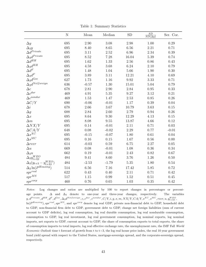
Table 1: Summary Statistics
N Mean Median SD SDSD(∆y) Ser. Cor.
∆y 695 2.90 3.08 2.98 1.00 0.29∆3y 695 8.40 8.65 6.56 2.21 0.71∆dPrivate 695 3.11 2.52 6.96 2.34 0.39∆3d
Private 695 8.52 7.28 16.04 5.39 0.74∆dHH 695 1.62 1.33 2.56 0.86 0.43∆3d
HH 695 4.58 3.68 6.24 2.10 0.79∆dF 695 1.48 1.04 5.66 1.90 0.30∆3d
F 695 3.89 3.11 12.21 4.10 0.69∆3d
Gov 627 1.73 1.16 9.92 3.33 0.71∆3d
Netforeign 636 -0.57 1.30 15.01 5.04 0.79∆c 678 2.81 2.90 2.84 0.95 0.33∆cdur 469 4.91 5.35 9.27 3.12 0.21∆cnondur 469 1.53 1.47 2.53 0.85 0.26∆C/Y 690 -0.06 -0.01 1.17 0.39 0.04∆i 678 2.66 3.67 10.79 3.63 0.15∆g 688 2.84 2.60 2.79 0.94 0.26∆x 695 8.64 9.30 12.29 4.13 0.15∆m 695 8.08 9.55 13.87 4.66 0.12∆NX/Y 695 0.14 -0.01 2.11 0.71 0.03∆CA/Y 648 0.08 -0.02 2.29 0.77 -0.01∆sXC 695 -0.15 -0.07 1.80 0.61 0.04∆sMC 695 0.16 0.15 1.67 0.56 0.00∆reer 614 -0.03 0.59 6.75 2.27 0.05∆u 669 0.08 -0.01 1.08 0.36 0.34∆3u 662 0.19 -0.01 2.43 0.82 0.67∆3y
WEOt+3|t 484 9.41 8.60 3.76 1.26 0.50
∆3(yt+3 − yWEOt+3|t ) 484 -2.53 -1.79 5.35 1.80 0.54
∆3 ln(PHousing) 514 6.56 7.16 17.42 5.85 0.72sprreal 622 0.43 0.40 2.11 0.71 0.42sprMS 517 1.15 0.99 1.52 0.51 0.45sprcorp 460 0.76 0.65 1.03 0.35 0.42
Notes: Log changes and ratios are multiplied by 100 to report changes in percentages or percent-age points. ∆ and ∆3 denote to one-year and three-year changes, respectively. The variablesy, dPrivate, dHH , dF , dGov,∆3d
Netforeign, c, cdur, cnondur, C/Y, i, g, x,m,NX/Y,CA/Y, sXC , sMC , reer, u, yWEOt+3|t ,
ln(PHousing), sprreal, sprMS , and sprcorp denote log real GDP, private non-financial debt to GDP, household debtto GDP, non-financial firm debt to GDP, government debt to GDP, change net foreign liabilities (sum of currentaccount to GDP deficits), log real consumption, log real durable consumption, log real nondurable consumption,consumption to GDP, log real investment, log real government consumption, log nominal exports, log nominalimports, net exports to GDP, current account to GDP, the share of consumption exports to total exports, the shareof consumption imports to total imports, log real effective exchange rate, the unemployment rate, the IMF Fall WorldEconomic Outlook time t forecast of growth from t to t+3, the log real house price index, the real 10 year governmentbond yield spread with respect to the United States, mortgage-sovereign spread, and the corporate-sovereign spread,respectively.
43
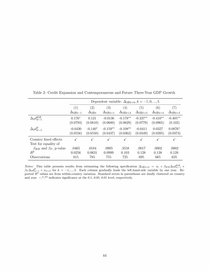
Table 2: Credit Expansion and Contemporaneous and Future Three-Year GDP Growth
Dependent variable: ∆3yit+k, k = −1, 0, ..., 5
(1) (2) (3) (4) (5) (6) (7)∆3yit−1 ∆3yit ∆3yit+1 ∆3yit+2 ∆3yit+3 ∆3yit+4 ∆3yit+5
∆3dHHit−1 0.176∗ 0.121 -0.0136 -0.178∗∗ -0.337∗∗ -0.410∗∗ -0.405∗∗
(0.0793) (0.0810) (0.0680) (0.0629) (0.0779) (0.0905) (0.102)
∆3dFit−1 -0.0430 -0.140∗ -0.159∗∗ -0.108∗∗ -0.0411 0.0327 0.0876∗
(0.0556) (0.0550) (0.0437) (0.0362) (0.0349) (0.0395) (0.0373)
Country fixed effects X X X X X X XTest for equality ofβHH and βF , p-value .0465 .0184 .0905 .3558 .0017 .0002 .0002
R2 0.0256 0.0631 0.0999 0.103 0.128 0.138 0.128Observations 815 785 755 725 695 665 635
Notes: This table presents results from estimating the following specification ∆3yit+k = αi + βHH∆3dHHit−1 +
βF ∆3dFit−1 + uit+k for k = −1, ..., 5. Each column gradually leads the left-hand-side variable by one year. Re-
ported R2 values are from within-country variation. Standard errors in parentheses are dually clustered on countryand year. +,*,** indicates significance at the 0.1, 0.05, 0.01 level, respectively.
44
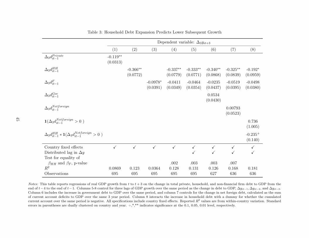
Table 3: Household Debt Expansion Predicts Lower Subsequent Growth
Dependent variable: ∆3yit+3
(1) (2) (3) (4) (5) (6) (7) (8)
∆3dPrivateit−1 -0.119∗∗
(0.0313)
∆3dHHit−1 -0.366∗∗ -0.337∗∗ -0.333∗∗ -0.340∗∗ -0.325∗∗ -0.192∗
(0.0772) (0.0779) (0.0771) (0.0868) (0.0839) (0.0959)
∆3dFit−1 -0.0978∗ -0.0411 -0.0464 -0.0235 -0.0519 -0.0498
(0.0391) (0.0349) (0.0354) (0.0437) (0.0395) (0.0380)
∆3dGovit−1 0.0534
(0.0430)
∆3dNetforeignit−1 0.00793
(0.0523)
1(∆3dNetforeignit−1 > 0 ) 0.736
(1.005)
∆3dHHit−1 ∗ 1(∆3d
Netforeignit−1 > 0 ) -0.235+
(0.140)
Country fixed effects X X X X X X X XDistributed lag in ∆y X X X XTest for equality ofβHH and βF , p-value .002 .003 .003 .007
R2 0.0869 0.123 0.0364 0.128 0.131 0.126 0.168 0.181Observations 695 695 695 695 695 627 636 636
Notes: This table reports regressions of real GDP growth from t to t+ 3 on the change in total private, household, and non-financial firm debt to GDP from theend of t−4 to the end of t−1. Columns 5-8 control for three lags of GDP growth over the same period as the change in debt to GDP, ∆yit−1,∆yit−2, and ∆yit−3.Column 6 includes the increase in government debt to GDP over the same period, and column 7 controls for the change in net foreign debt, calculated as the sumof current account deficits to GDP over the same 3 year period. Column 8 interacts the increase in household debt with a dummy for whether the cumulatedcurrent account over the same period is negative. All specifications include country fixed effects. Reported R2 values are from within-country variation. Standarderrors in parentheses are dually clustered on country and year. +,*,** indicates significance at the 0.1, 0.05, 0.01 level, respectively.
45

Table 4: Household Debt Expansion Predicts Lower Growth: Robustness and Subsamples
Panel A: Robustness to Alternative SpecificationsDependent variable: ∆3yit+3
(1) (2) (3) (4) (5) (6) (7)OLS AB-GMM OLS MBB SE OLS OLS OLS
∆3dHHit−1 -0.32∗∗ -0.32∗∗ -0.31∗∗ -0.33∗∗ -0.23∗∗ -0.21∗∗
(0.081) (0.11) (0.087) (0.083) (0.075) (0.063)
∆3dFit−1 -0.057 -0.069 -0.063 -0.046 -0.042 -0.037
(0.044) (0.071) (0.045) (0.031) (0.033) (0.033)
Trend -0.23∗∗
(0.063)
∆3dHHit−1, alt norm. -0.30∗∗
(0.070)
∆3dFit−1, alt. norm. 0.020
(0.034)
Country fixed effects X X X X XDistributed lag in ∆y X X X X X X XYear fixed effects XSample Non-overl. Non-overl. Full Full Full. Full FullTest for equality ofβHH and βF , p-value .007 .0004 .035 .0043 .031 .012 .0002
R2 0.15 0.18 0.13 0.26 0.50 0.15Observations 232 203 695 695 695 695 695
Panel B: SubsamplesDependent variable: ∆3yit+3
(1) (2) (3) (4) (5) (6)
∆3dHHit−1 -0.37∗∗ -0.24∗∗ -0.29∗∗ -0.22∗∗ -0.19∗∗ -0.16∗∗
(0.097) (0.070) (0.10) (0.054) (0.072) (0.057)
∆3dFit−1 -0.027 -0.069 -0.038 -0.053 -0.055 -0.061
(0.040) (0.063) (0.062) (0.039) (0.038) (0.038)
Trend -0.16∗
(0.066)
Country fixed effects X X X X X XDistributed lag in ∆y X X X X X XYear fixed effects XSample Developed Emerging Pre 1995 Pre 2006 Pre 2006 Pre 2006Test for equality ofβHH and βF , p-value .005 .082 .009 .021 .116 .17
R2 0.16 0.11 0.13 0.088 0.16 0.37Observations 529 166 259 517 517 517
Notes: Panel A presents a variety of robustness tests of the main specification in Table 3. Column 1 uses the non-overlapping samplethat only includes every third year. This specification controls for ∆3yit−1. Column 2 uses the Arellano-Bond GMM estimatorfor the equation in differences on the same non-overlapping sample. We instrument for ∆3d
HHit−1 and ∆3d
Fit−1 with a double lag,
∆3dHHit−4 and ∆3d
Fit−4. Column 3 omits country fixed effects from the main specification estimated using the full sample. Column
4 computes standard errors using the panel moving blocks bootstrap (Gonçalves (2011)) with a block length of l = 3. Column 5includes a time trend, and column 6 includes country fixed effects. Column 7 replace the three year change in debt to GDP withthe change in debt normalized by initial (t− 4) GDP.Panel B reports estimates on various subsamples. Columns 1 and 2 present separate estimates for developed and emerging economies.Emerging market economies are the Czech Republic, Hong Kong, Hungary, Indonesia, Korea, Mexico, Poland, Singapore, Thailand,and Turkey. Developed economies are the remaining countries. Column 3 uses data up to 1995, and columns 4-6 use data up to2006. Column 5 includes a time trend, and column 6 controls for year fixed effects.Standard errors in all columns (except panel A column 4) are dually clustered on country and year. Reported R2 values in regressionsincluding country fixed effects are from within-country variation. +,*,** indicates significance at the 0.1, 0.05, 0.01 level, respectively.
46
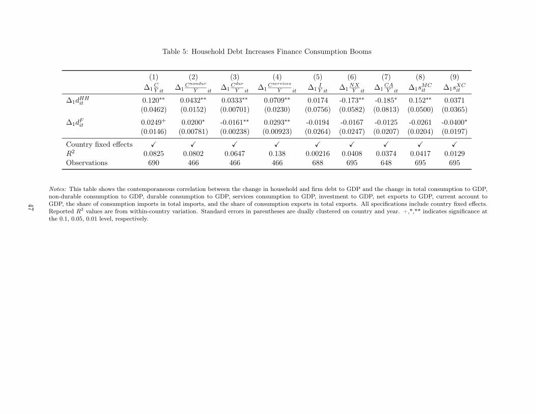
Table 5: Household Debt Increases Finance Consumption Booms
(1) (2) (3) (4) (5) (6) (7) (8) (9)∆1
CY it
∆1Cnondur
Y it∆1
Cdur
Y it∆1
Cservices
Y it∆1
IY it
∆1NXY it
∆1CAY it
∆1sMCit ∆1s
XCit
∆1dHHit 0.120∗∗ 0.0432∗∗ 0.0333∗∗ 0.0709∗∗ 0.0174 -0.173∗∗ -0.185∗ 0.152∗∗ 0.0371
(0.0462) (0.0152) (0.00701) (0.0230) (0.0756) (0.0582) (0.0813) (0.0500) (0.0365)
∆1dFit 0.0249+ 0.0200∗ -0.0161∗∗ 0.0293∗∗ -0.0194 -0.0167 -0.0125 -0.0261 -0.0400∗
(0.0146) (0.00781) (0.00238) (0.00923) (0.0264) (0.0247) (0.0207) (0.0204) (0.0197)
Country fixed effects X X X X X X X X XR2 0.0825 0.0802 0.0647 0.138 0.00216 0.0408 0.0374 0.0417 0.0129Observations 690 466 466 466 688 695 648 695 695
Notes: This table shows the contemporaneous correlation between the change in household and firm debt to GDP and the change in total consumption to GDP,non-durable consumption to GDP, durable consumption to GDP, services consumption to GDP, investment to GDP, net exports to GDP, current account toGDP, the share of consumption imports in total imports, and the share of consumption exports in total exports. All specifications include country fixed effects.Reported R2 values are from within-country variation. Standard errors in parentheses are dually clustered on country and year. +,*,** indicates significance atthe 0.1, 0.05, 0.01 level, respectively.
47
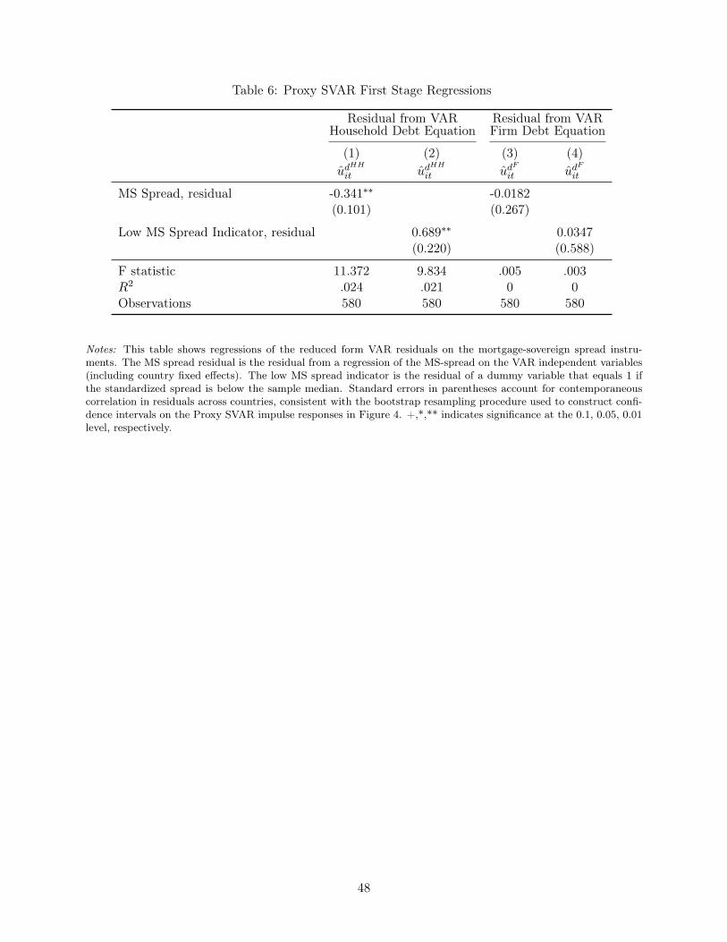
Table 6: Proxy SVAR First Stage Regressions
Residual from VARHousehold Debt Equation
Residual from VARFirm Debt Equation
(1) (2) (3) (4)ud
HH
it udHH
it udF
it udF
it
MS Spread, residual -0.341∗∗ -0.0182(0.101) (0.267)
Low MS Spread Indicator, residual 0.689∗∗ 0.0347(0.220) (0.588)
F statistic 11.372 9.834 .005 .003R2 .024 .021 0 0Observations 580 580 580 580
Notes: This table shows regressions of the reduced form VAR residuals on the mortgage-sovereign spread instru-ments. The MS spread residual is the residual from a regression of the MS-spread on the VAR independent variables(including country fixed effects). The low MS spread indicator is the residual of a dummy variable that equals 1 ifthe standardized spread is below the sample median. Standard errors in parentheses account for contemporaneouscorrelation in residuals across countries, consistent with the bootstrap resampling procedure used to construct confi-dence intervals on the Proxy SVAR impulse responses in Figure 4. +,*,** indicates significance at the 0.1, 0.05, 0.01level, respectively.
48
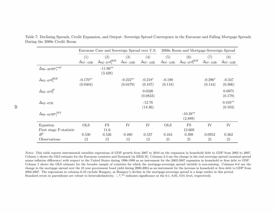
Table 7: Declining Spreads, Credit Expansion, and Output: Sovereign Spread Convergence in the Eurozone and Falling Mortgage SpreadsDuring the 2000s Credit Boom
Eurozone Case and Sovereign Spread over U.S. 2000s Boom and Mortgage-Sovereign Spread
(1) (2) (3) (4) (5) (6) (7) (8)∆07−10yi ∆02−07d
HHi ∆07−10yi ∆07−10yi ∆07−10yi ∆02−07d
HHi ∆07−10yi ∆07−10yi
∆96−99sprreali -11.66∗∗
(3.428)
∆02−07dHHi -0.170∗∗ -0.222∗∗ -0.218∗ -0.180 -0.296∗ -0.347
(0.0404) (0.0479) (0.107) (0.118) (0.144) (0.306)
∆02−07dFi 0.0326 0.0975
(0.0833) (0.179)
∆02−07yi -12.76 0.416∗∗
(14.36) (0.103)
∆00−04sprMSi -10.28∗∗
(2.889)
Equation OLS FS IV IV OLS FS IV IVFirst stage F-statistic 11.6 12.669R2 0.530 0.526 0.480 0.537 0.164 0.398 0.0952 0.362Observations 12 12 12 12 21 21 21 21
Notes: This table reports instrumental variables regressions of GDP growth from 2007 to 2010 on the expansion in household debt to GDP from 2002 to 2007.Column 1 shows the OLS estimate for the Eurozone countries and Denmark (in ERM II). Columns 2-4 use the change in the real sovereign spread (nominal spreadminus inflation difference) with respect to the United States during 1996-1999 as an instrument for the 2002-2007 expansion in household or firm debt to GDP.Column 5 shows the OLS estimate for the broader sample of countries for which the mortgage-sovereign spread variable is non-missing. Columns 6-8 use thechange in the mortgage spread over the 10 year government bond yield during 2000-2004 as an instrument for the increase in household or firm debt to GDP from2002-2007. The regressions in columns 6-10 exclude Hungary, as Hungary’s decline in the mortgage-sovereign spread is a large outlier in this period.Standard errors in parentheses are robust to heteroskedasticity. +,*,** indicates significance at the 0.1, 0.05, 0.01 level, respectively.
49

Table 8: Rise in Household Debt Predicts Overoptimistic IMF and OECD Growth Forecasts
Growth Forecast Forecast ErrorForecast Error
Sample up to 2006
(1) (2) (3) (4) (5) (6) (7) (8) (9)∆2y
IMFt+2|t ∆2y
OECDt+2|t eIMF
t+1|t eIMFt+2|t eIMF
t+3|t eOECDt+1|t eOECD
t+2|t eIMFt+1|t eOECD
t+1|t
∆3dHHit−1 0.0016 0.0013 -0.060∗∗ -0.17∗∗ -0.31∗∗ -0.070∗∗ -0.17∗ -0.035+ -0.042∗∗
(0.023) (0.028) (0.020) (0.057) (0.091) (0.023) (0.071) (0.021) (0.015)
∆3dFit−1 -0.029 -0.041∗ -0.019 -0.026 -0.031 -0.013 -0.0084 -0.029 -0.020∗
(0.021) (0.017) (0.027) (0.045) (0.051) (0.015) (0.029) (0.020) (0.0080)
Country fixed effects X X X X X X X X XSample Full Full Full Full Full Full Full Pre 2006 Pre 2006Test for equality ofβHH and βF , p-value .367 .227 .311 .089 .02 .053 .07 .863 .29
R2 0.034 0.064 0.026 0.063 0.13 0.040 0.073 0.026 0.027Observations 484 471 590 484 484 594 471 469 490
Notes: This table reports regression estimates of GDP growth forecasts and forecast errors on the change in household and non-financial firm debt to GDP fromt − 4 to t − 1. The forecasts are from the fall issues of the IMF World Economic Outlook and the OECD Economic Outlook. ∆hy
ft+h|t is the forecasted change
in log GDP from t to t + h made in the Fall of year t, and eft+h|t is the realized forecast error. The IMF and OECD forecast errors are constructed using therealized log GDP change reported in the IMF’s Historical WEO Forecasts Database and the OECD Economic Outlook reports, respectively. The World EconomicOutlook forecast sample includes all 30 countries in the sample and covers the years 1990-2012, with one-year-ahead forecasts extending back to 1972 for the G7.One- and two-year-ahead OECD Economic Outlook forecasts are for years 1973-2012 and 1987-2012, respectively. We exclude Hong Kong, Indonesia, Singapore,and Thailand from the OECD sample because of gaps in the forecast series. The regressions in columns 8 and 9 are estimated using data to 2006.Reported R2 values are from within-country variation. Standard errors in parentheses are dually clustered on country and year. +,*,** indicates significance atthe 0.1, 0.05, 0.01 level, respectively.
50
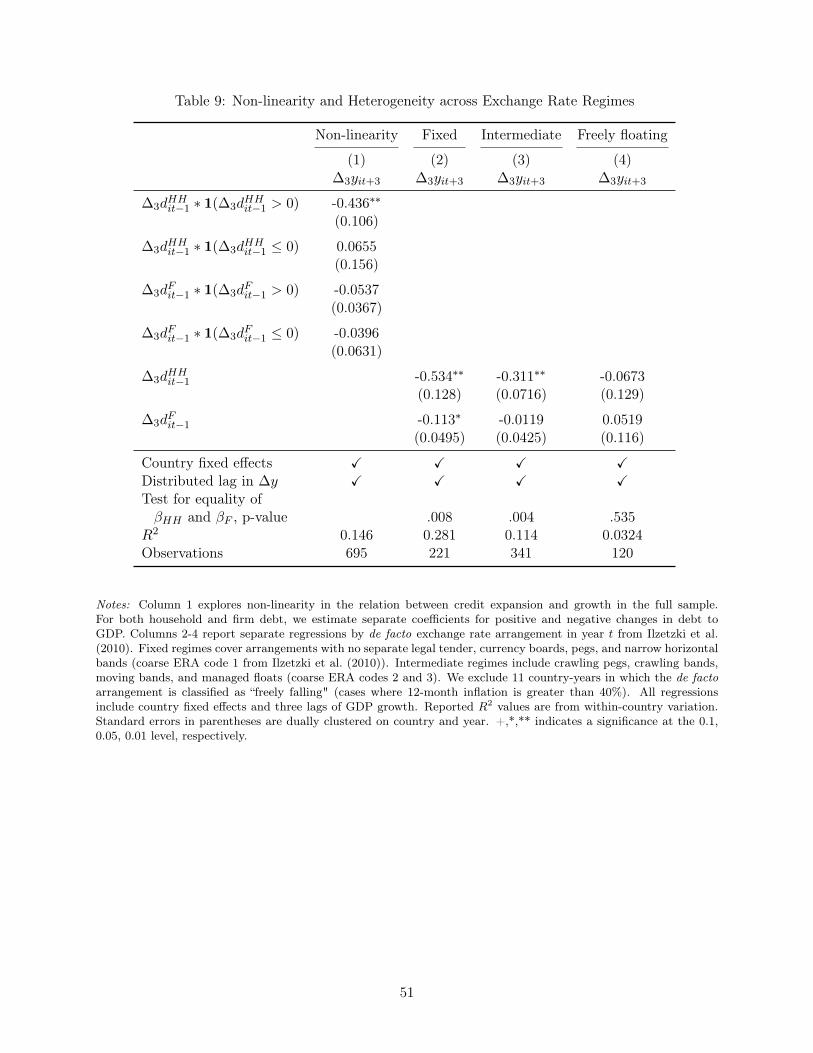
Table 9: Non-linearity and Heterogeneity across Exchange Rate Regimes
Non-linearity Fixed Intermediate Freely floating
(1) (2) (3) (4)∆3yit+3 ∆3yit+3 ∆3yit+3 ∆3yit+3
∆3dHHit−1 ∗ 1(∆3d
HHit−1 > 0) -0.436∗∗
(0.106)
∆3dHHit−1 ∗ 1(∆3d
HHit−1 ≤ 0) 0.0655
(0.156)
∆3dFit−1 ∗ 1(∆3d
Fit−1 > 0) -0.0537
(0.0367)
∆3dFit−1 ∗ 1(∆3d
Fit−1 ≤ 0) -0.0396
(0.0631)
∆3dHHit−1 -0.534∗∗ -0.311∗∗ -0.0673
(0.128) (0.0716) (0.129)
∆3dFit−1 -0.113∗ -0.0119 0.0519
(0.0495) (0.0425) (0.116)
Country fixed effects X X X XDistributed lag in ∆y X X X XTest for equality ofβHH and βF , p-value .008 .004 .535
R2 0.146 0.281 0.114 0.0324Observations 695 221 341 120
Notes: Column 1 explores non-linearity in the relation between credit expansion and growth in the full sample.For both household and firm debt, we estimate separate coefficients for positive and negative changes in debt toGDP. Columns 2-4 report separate regressions by de facto exchange rate arrangement in year t from Ilzetzki et al.(2010). Fixed regimes cover arrangements with no separate legal tender, currency boards, pegs, and narrow horizontalbands (coarse ERA code 1 from Ilzetzki et al. (2010)). Intermediate regimes include crawling pegs, crawling bands,moving bands, and managed floats (coarse ERA codes 2 and 3). We exclude 11 country-years in which the de factoarrangement is classified as “freely falling" (cases where 12-month inflation is greater than 40%). All regressionsinclude country fixed effects and three lags of GDP growth. Reported R2 values are from within-country variation.Standard errors in parentheses are dually clustered on country and year. +,*,** indicates a significance at the 0.1,0.05, 0.01 level, respectively.
51

Table 10: Unemployment and Household Debt Expansions
Full SampleFixed ERRegimes Intermediate Freely floating
(1) (2) (3) (4) (5)∆3uit+3 ∆3uit+3 ∆3uit+3 ∆3uit+3 ∆3uit+3
∆3dHHit−1 0.132∗∗ 0.105∗∗ 0.264∗∗ 0.0709+ -0.0159
(0.0380) (0.0390) (0.0736) (0.0367) (0.0587)
∆3dFit−1 0.0363∗ 0.0373∗ 0.0615+ 0.0385∗ 0.0403
(0.0153) (0.0158) (0.0319) (0.0194) (0.0332)
Country fixed effects X X X X XDistributed lag in ∆u X X X XTest for equality ofβHH and βF , p-value .026 .131 .001 .425 .506
R2 0.145 0.207 0.397 0.235 0.254Observations 662 638 211 296 120
Notes: This table reports regression estimates of the change in the unemployment rate from t to t+3 on the change inhousehold and non-financial firm debt to GDP from t−4 to t−1. All columns include country fixed effects. Columns2-5 include three lags of the change in the unemployment rate as controls. Columns 3-5 estimate the regression acrossexchange rate regimes, as defined in Table 9. Reported R2 values are from within-country variation. Standard errorsin parentheses are dually clustered on country and year. +,*,** indicates significance at the 0.1, 0.05, 0.01 level,respectively.
52
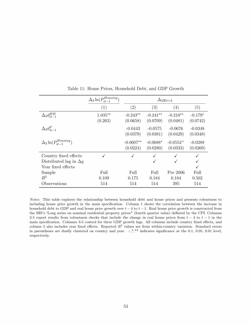
Table 11: House Prices, Household Debt, and GDP Growth
∆3 ln(PHousingit−1 ) ∆3yit+3
(1) (2) (3) (4) (5)
∆3dHHit−1 1.035∗∗ -0.243∗∗ -0.241∗∗ -0.210∗∗ -0.179∗
(0.263) (0.0658) (0.0709) (0.0481) (0.0742)
∆3dFit−1 -0.0443 -0.0575 -0.0676 -0.0348
(0.0379) (0.0381) (0.0429) (0.0348)
∆3 ln(PHousingit−1 ) -0.0607∗∗ -0.0688∗ -0.0552+ -0.0288
(0.0224) (0.0280) (0.0333) (0.0269)
Country fixed effects X X X X XDistributed lag in ∆y X X XYear fixed effects XSample Full Full Full Pre 2006 FullR2 0.109 0.175 0.184 0.184 0.502Observations 514 514 514 395 514
Notes: This table explores the relationship between household debt and house prices and presents robustness toincluding house price growth in the main specification. Column 1 shows the correlation between the increase inhousehold debt to GDP and real house price growth over t− 4 to t− 1. Real house price growth is constructed fromthe BIS’s “Long series on nominal residential property prices" (fourth quarter value) deflated by the CPI. Columns2-5 report results from robustness checks that include the change in real house prices from t − 4 to t − 1 in themain specification. Columns 3-5 control for three GDP growth lags. All columns include country fixed effects, andcolumn 5 also includes year fixed effects. Reported R2 values are from within-country variation. Standard errorsin parentheses are dually clustered on country and year. +,*,** indicates significance at the 0.1, 0.05, 0.01 level,respectively.
53
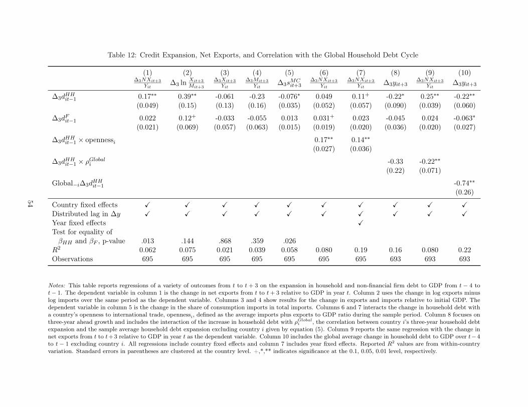
Table 12: Credit Expansion, Net Exports, and Correlation with the Global Household Debt Cycle
(1) (2) (3) (4) (5) (6) (7) (8) (9) (10)∆3NXit+3
Yit∆3 ln Xit+3
Mit+3
∆3Xit+3
Yit
∆3Mit+3
Yit∆3s
MCit+3
∆3NXit+3
Yit
∆3NXit+3
Yit∆3yit+3
∆3NXit+3
Yit∆3yit+3
∆3dHHit−1 0.17∗∗ 0.39∗∗ -0.061 -0.23 -0.076∗ 0.049 0.11+ -0.22∗ 0.25∗∗ -0.22∗∗
(0.049) (0.15) (0.13) (0.16) (0.035) (0.052) (0.057) (0.090) (0.039) (0.060)
∆3dFit−1 0.022 0.12+ -0.033 -0.055 0.013 0.031+ 0.023 -0.045 0.024 -0.063∗
(0.021) (0.069) (0.057) (0.063) (0.015) (0.019) (0.020) (0.036) (0.020) (0.027)
∆3dHHit−1 × opennessi 0.17∗∗ 0.14∗∗
(0.027) (0.036)
∆3dHHit−1 × ρGlobal
i -0.33 -0.22∗∗
(0.22) (0.071)
Global−i∆3dHHit−1 -0.74∗∗
(0.26)
Country fixed effects X X X X X X X X X XDistributed lag in ∆y X X X X X X X X X XYear fixed effects XTest for equality ofβHH and βF , p-value .013 .144 .868 .359 .026
R2 0.062 0.075 0.021 0.039 0.058 0.080 0.19 0.16 0.080 0.22Observations 695 695 695 695 695 695 695 693 693 693
Notes: This table reports regressions of a variety of outcomes from t to t + 3 on the expansion in household and non-financial firm debt to GDP from t − 4 tot− 1. The dependent variable in column 1 is the change in net exports from t to t+ 3 relative to GDP in year t. Column 2 uses the change in log exports minuslog imports over the same period as the dependent variable. Columns 3 and 4 show results for the change in exports and imports relative to initial GDP. Thedependent variable in column 5 is the change in the share of consumption imports in total imports. Columns 6 and 7 interacts the change in household debt witha country’s openness to international trade, opennessi, defined as the average imports plus exports to GDP ratio during the sample period. Column 8 focuses onthree-year ahead growth and includes the interaction of the increase in household debt with ρGlobal
i , the correlation between country i’s three-year household debtexpansion and the sample average household debt expansion excluding country i given by equation (5). Column 9 reports the same regression with the change innet exports from t to t+3 relative to GDP in year t as the dependent variable. Column 10 includes the global average change in household debt to GDP over t−4to t − 1 excluding country i. All regressions include country fixed effects and column 7 includes year fixed effects. Reported R2 values are from within-countryvariation. Standard errors in parentheses are clustered at the country level. +,*,** indicates significance at the 0.1, 0.05, 0.01 level, respectively.
54
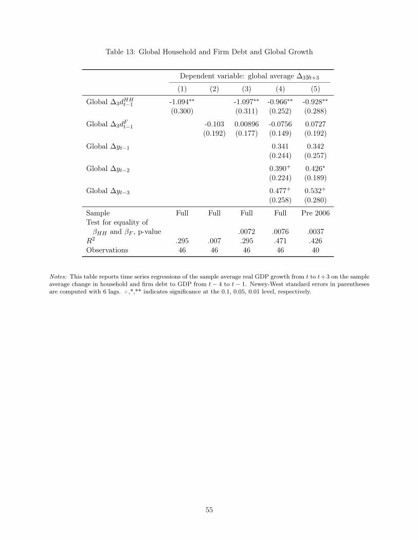
Table 13: Global Household and Firm Debt and Global Growth
Dependent variable: global average ∆3yt+3
(1) (2) (3) (4) (5)
Global ∆3dHHt−1 -1.094∗∗ -1.097∗∗ -0.966∗∗ -0.928∗∗
(0.300) (0.311) (0.252) (0.288)
Global ∆3dFt−1 -0.103 0.00896 -0.0756 0.0727
(0.192) (0.177) (0.149) (0.192)
Global ∆yt−1 0.341 0.342(0.244) (0.257)
Global ∆yt−2 0.390+ 0.426∗
(0.224) (0.189)
Global ∆yt−3 0.477+ 0.532+
(0.258) (0.280)
Sample Full Full Full Full Pre 2006Test for equality ofβHH and βF , p-value .0072 .0076 .0037
R2 .295 .007 .295 .471 .426Observations 46 46 46 46 40
Notes: This table reports time series regressions of the sample average real GDP growth from t to t+3 on the sampleaverage change in household and firm debt to GDP from t− 4 to t− 1. Newey-West standard errors in parenthesesare computed with 6 lags. +,*,** indicates significance at the 0.1, 0.05, 0.01 level, respectively.
55
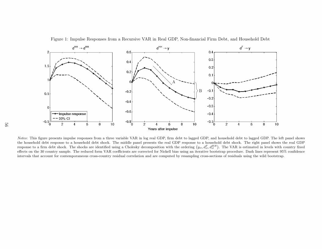
Figure 1: Impulse Responses from a Recursive VAR in Real GDP, Non-financial Firm Debt, and Household Debt
A
B
Notes: This figure presents impulse responses from a three variable VAR in log real GDP, firm debt to lagged GDP, and household debt to lagged GDP. The left panel showsthe household debt response to a household debt shock. The middle panel presents the real GDP response to a household debt shock. The right panel shows the real GDPresponse to a firm debt shock. The shocks are identified using a Cholesky decomposition with the ordering
(yit, d
Fit, d
HHit
). The VAR is estimated in levels with country fixed
effects on the 30 country sample. The reduced form VAR coefficients are corrected for Nickell bias using an iterative bootstrap procedure. Dash lines represent 95% confidenceintervals that account for contemporaneous cross-country residual correlation and are computed by resampling cross-sections of residuals using the wild bootstrap.
56
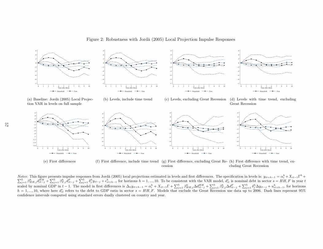
Figure 2: Robustness with Jordà (2005) Local Projection Impulse Responses
-1
-.8
-.6
-.4
-.2
0
.2
.4
.6
0 1 2 3 4 5 6 7 8 9 10Years after shock
Household Firm
(a) Baseline: Jordà (2005) Local Projec-tion VAR in levels on full sample
-1
-.8
-.6
-.4
-.2
0
.2
.4
.6
0 1 2 3 4 5 6 7 8 9 10Years after shock
Household Firm
(b) Levels, include time trend
-1
-.8
-.6
-.4
-.2
0
.2
.4
.6
0 1 2 3 4 5 6 7 8 9 10Years after shock
Household Firm
(c) Levels, excluding Great Recession
-1
-.8
-.6
-.4
-.2
0
.2
.4
.6
0 1 2 3 4 5 6 7 8 9 10Years after shock
Household Firm
(d) Levels with time trend, excludingGreat Recession
-1.6
-1.4
-1.2
-1
-.8
-.6
-.4
-.2
0
.2
.4
.6
0 1 2 3 4 5 6 7 8 9 10Years after shock
Household Firm
(e) First differences
-1
-.8
-.6
-.4
-.2
0
.2
.4
.6
0 1 2 3 4 5 6 7 8 9 10Years after shock
Household Firm
(f) First difference, include time trend
-1
-.8
-.6
-.4
-.2
0
.2
.4
.6
0 1 2 3 4 5 6 7 8 9 10Years after shock
Household Firm
(g) First difference, excluding Great Re-cession
-1
-.8
-.6
-.4
-.2
0
.2
.4
.6
0 1 2 3 4 5 6 7 8 9 10Years after shock
Household Firm
(h) First difference with time trend, ex-cluding Great Recession
Notes: This figure presents impulse responses from Jordà (2005) local projections estimated in levels and first differences. The specification in levels is: yit+h−1 = αhi +Xit−1Γh +∑5
j=1 βhHH,jd
HHit−j +
∑5j=1 β
hF,jd
Fit−j +
∑5j=1 δ
hj yit−j + εhit+h−1 for horizons h = 1, ..., 10. To be consistent with the VAR model, dsit is nominal debt in sector s = HH,F in year t
scaled by nominal GDP in t− 1. The model in first differences is ∆hyit+h−1 = αhi +Xit−1Γ +
∑5j=1 β
hHH,j∆d
HHit−j +
∑5j=1 β
hF,j∆d
Fit−j +
∑5j=1 δ
hj ∆yit−j + uh
it+h−1, for horizonsh = 1, ..., 10, where here dsit refers to the debt to GDP ratio in sector s = HH,F . Models that exclude the Great Recession use data up to 2006. Dash lines represent 95%confidence intervals computed using standard errors dually clustered on country and year.
57
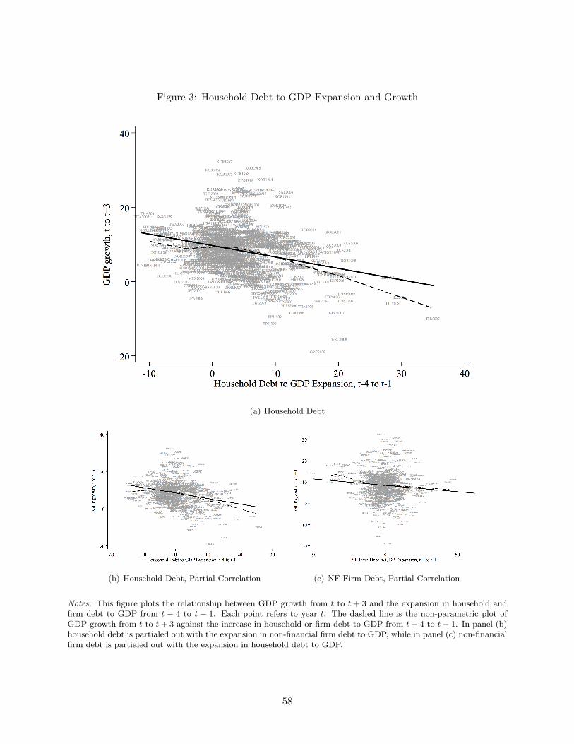
Figure 3: Household Debt to GDP Expansion and Growth
(a) Household Debt
(b) Household Debt, Partial Correlation (c) NF Firm Debt, Partial Correlation
Notes: This figure plots the relationship between GDP growth from t to t + 3 and the expansion in household andfirm debt to GDP from t − 4 to t − 1. Each point refers to year t. The dashed line is the non-parametric plot ofGDP growth from t to t+ 3 against the increase in household or firm debt to GDP from t− 4 to t− 1. In panel (b)household debt is partialed out with the expansion in non-financial firm debt to GDP, while in panel (c) non-financialfirm debt is partialed out with the expansion in household debt to GDP.
58

Figure 4: Impulse Responses to a Household Debt Shock Identified with the Mortgage Lending Spread in a Proxy SVAR
Notes: This figure shows impulse responses to a household debt shock identified using an indicator variable for whether the standardized mortgage spread is below the medianas an external instrument in a Proxy SVAR. The reduced form VAR coefficient estimates are corrected for Nickell bias using an iterative bootstrap procedure. Dash linesrepresent 95% confidence intervals that account for contemporaneous cross-country residual correlation and are computed by resampling cross-sections of residuals using thewild bootstrap.
59
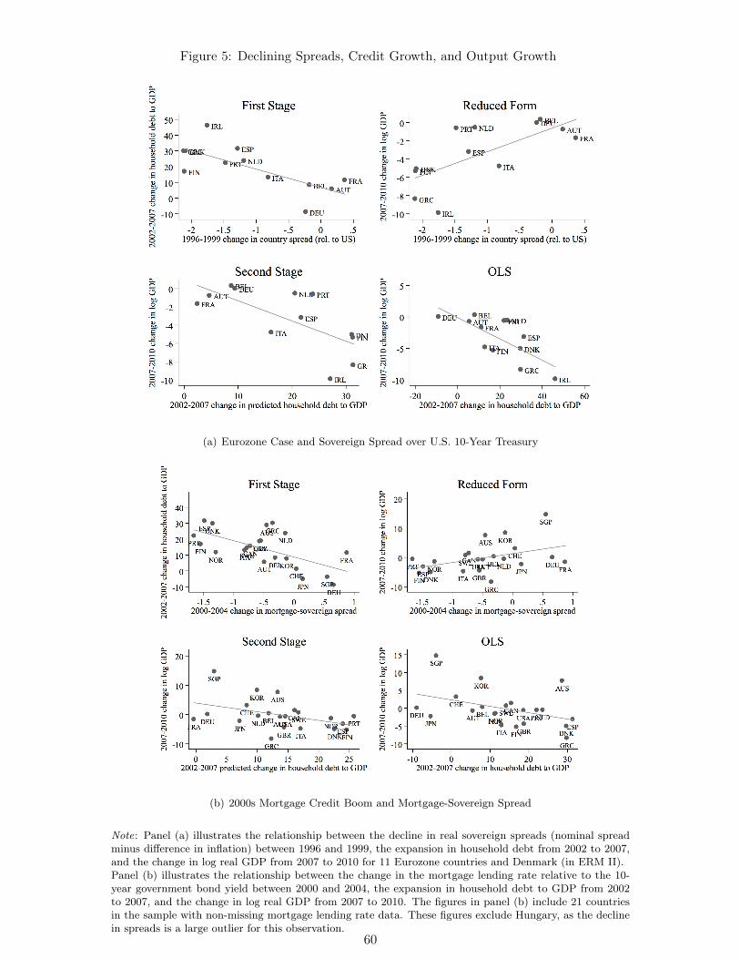
Figure 5: Declining Spreads, Credit Growth, and Output Growth
(a) Eurozone Case and Sovereign Spread over U.S. 10-Year Treasury
(b) 2000s Mortgage Credit Boom and Mortgage-Sovereign Spread
Note: Panel (a) illustrates the relationship between the decline in real sovereign spreads (nominal spreadminus difference in inflation) between 1996 and 1999, the expansion in household debt from 2002 to 2007,and the change in log real GDP from 2007 to 2010 for 11 Eurozone countries and Denmark (in ERM II).Panel (b) illustrates the relationship between the change in the mortgage lending rate relative to the 10-year government bond yield between 2000 and 2004, the expansion in household debt to GDP from 2002to 2007, and the change in log real GDP from 2007 to 2010. The figures in panel (b) include 21 countriesin the sample with non-missing mortgage lending rate data. These figures exclude Hungary, as the declinein spreads is a large outlier for this observation.
60
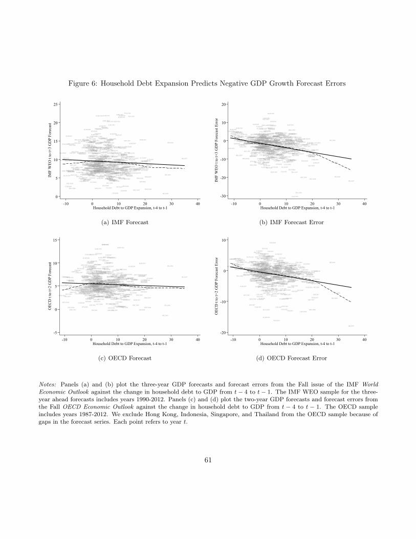
Figure 6: Household Debt Expansion Predicts Negative GDP Growth Forecast Errors
THA2002
HUN1993
NOR1994
THA2001
FIN1996
HUN1994
FIN1997
CHE2009
SGP2007
NOR1996
DEU2009
SWE1996NOR1995
HKG2007
NOR1993
DEU2008
SGP2008
FIN1998
FIN1995
SWE1997
SWE1992
SWE1993
HKG2008
NOR1997NOR1992
THA2003
HKG2006
FIN1999
SWE1995
DEU2007
SWE1994
NOR1998
HUN1997
JPN2005
HUN1998
HKG2009
CHE2008
CZE1999
HUN1996
JPN2003
JPN2004
JPN2007
HKG2005
JPN2009
SWE1998
GBR1997
JPN2006
MEX1999MEX2000
GBR1996FRA1997
DEU1991
JPN2008
HUN1995
HUN1999
DEU2006
MEX2001
ITA1996
KOR2000
KOR2001
ITA1997
CAN1996
DEU1992
DEU2005
SGP2009
GBR1995
MEX2002
CAN2002
BEL2003
NOR2001
DEU1993
BEL2002FRA1998
TUR2004
DEU1990
JPN2002
ITA1998
DEU2004
HKG1995
FIN1994MEX1998
TUR1997
THA2009
TUR1991
FIN2000
DEU2003
CAN2001
ITA1992
CZE2000
TUR1990
FRA1996
GBR1998
TUR2003
ESP1993
NOR2002
CZE2001
ITA1995
HUN2000
BEL1996
TUR2002
FRA1999
TUR1992
THA2000
CHE2007
TUR1993
IDN2009
ESP1995ESP1996
THA2008
JPN1999
GBR1994
CHE2003
MEX2003
TUR2000
JPN1994
AUT2009
PRT1991
JPN1998
FRA2001
BEL2004
ITA1991
FRA2000
SGP2006
CAN1997
KOR2006
ESP1997
IDN2008
ESP1994
BEL2001
AUS1993
TUR1995TUR1999
KOR1999
PRT1992
ITA1990
NOR1999
TUR1996
BEL1997
USA1995
JPN1993ITA1994
NOR1991CAN2003
CZE2002
FRA1995
JPN2001
ITA1999
AUS1991
TUR2001
USA1994
CAN1995
LUX2007
SWE1999AUT1999
HUN2001
MEX2004
FRA2002
JPN2000AUT2004
FIN2001
GBR1999USA1999
TUR1998
BEL2005BEL1995ITA1993USA1998
MEX2005
FRA2003
USA2000
HKG2004
JPN1995FIN1993
ESP1992
CAN1998
AUS1992PRT1993
AUS1990
SGP2001
MEX2006
AUT2003USA1993
IDN2007
POL2006
JPN1997
TUR1994
SWE1991
NOR2000
MEX2009
THA2007
BEL1998
HKG1996
HKG2003
AUT2001
THA2004
POL2002
POL2000
MEX2007
POL2001
KOR1996
USA1996
PRT1990
AUT2000SWE2000
GRC1998
TUR2005
FRA1993
FRA2004USA1997
FIN2002
CAN2000
NOR2009
BEL1994
USA1992
BEL2000
AUT2008
AUS1994
FIN2003
FRA1994
AUT2005
ESP1998USA1991
JPN1996
USA1990
DEU1994
NOR2007
GRC1999
BEL1992GBR1993FRA1992
FIN1992
DEU2002
SGP2000
LUX2008
MEX2008
BEL1993
CZE2003
AUT2002ITA2000SWE2001
USA2001
BEL1999
KOR1997
GRC2000
SGP2005
POL1999
FRA1991
CZE2004
BEL1991
BEL2006
HUN2002
KOR1998
FRA1990
CAN1994
HKG1997
ESP1991
HKG2002
CAN1999
FRA2005
POL2005
IDN2006
LUX2006
SGP1999
NLD1994ITA2003USA2009
BEL1990
ITA2001
TUR2009
IDN2005
NLD2009
GBR2000ITA2004
SGP2003
KOR1994
CZE2006
KOR1995
JPN1992
HKG1994
ITA2002
CZE2005
POL2007
FIN1991
THA2006
DNK2002
GBR2001
TUR2006
CAN2004
BEL2007
AUS2009
AUT2007
POL2004
AUT2006
NOR2008
GRC2001
SWE2002
ITA2005
AUS1995
SWE2003
FRA2006
KOR2007
DEU2001
ITA2009
NOR2006
NOR2003
SGP2002
FIN2009
SGP1998
DEU1995
TUR2007
TUR2008
GBR1992
BEL2009
POL2003
LUX2009
DNK2001
THA2005
BEL2008
SGP1995
PRT1994
FIN2004
CHE2006
KOR2005
USA2002
ESP1999
SWE2004
HKG2001
HUN2003
DEU1998
NLD1995
GBR2008
CZE2007
FRA2009
KOR1993
FRA2007
ESP1990
ITA2006
SWE2005DEU1999
SWE1990
DEU1997CAN2005
CAN1993
THA1999
AUS1996
CHE2005
FRA2008
CHE2004
DEU2000CAN2006
KOR2002
DEU1996
GBR2009
JPN1991
CAN1992
AUS1998
SWE2008NLD1996
DNK2000
CAN2007
CAN1991
AUS1997
SWE2009
ITA2007
ITA2008
GBR2002
PRT1995NOR1990
FIN1990
GRC2002
CAN1990
FIN2008
KOR2009
SGP1996
ESP2003
POL2008
HUN2007
SWE2006
AUS1999ESP2002
USA2008
SWE2007
CZE2008
CZE2009FIN2005
SGP1997
GBR1991
DNK2003
ESP2000
PRT2009
CAN2008
KOR1990
HUN2008NLD1997
USA2007
USA2003
PRT1997
CAN2009
DNK1999
PRT1996
KOR2008
DNK1998
KOR1992
HUN2004
GBR2007
NLD2008
KOR1991
ESP2004ESP2001
SGP2004
FIN2007
NOR2005
AUS2001
GBR1990
ESP2009
GRC2003
NLD2003GBR2006
AUS2000
HUN2005AUS2002
HKG1998
HUN2006
THA1998
PRT1998
GBR2003FIN2006
DNK2004
PRT2008
USA2006
NLD1998GRC2004
JPN1990
THA1997
PRT2005
NLD2002AUS2008
THA1996
HUN2009PRT2007
HKG2000
PRT2004
USA2005
DNK2005
AUS2003
PRT2006
GRC2005
NOR2004
THA1995
HKG1999
USA2004
POL2009
PRT2003GBR2004
KOR2004
NLD2007NLD2004
PRT1999ESP2005
AUS2007
GRC2009
NLD1999
DNK2006
GBR2005
GRC2006
NLD2001NLD2005
DNK2009
NLD2000
ESP2008
KOR2003
AUS2004
GRC2007
PRT2002
ESP2006PRT2000
NLD2006GRC2008
AUS2006
DNK2008
DNK2007
ESP2007PRT2001
AUS2005
IRL2009
IRL2008
IRL2006
IRL2007
0
5
10
15
20
25
IMF
WEO
t to
t+3
GD
P Fo
reca
st
-10 0 10 20 30 40Household Debt to GDP Expansion, t-4 to t-1
(a) IMF Forecast
THA2002
HUN1993
NOR1994
THA2001FIN1996
HUN1994
FIN1997
CHE2009
SGP2007
NOR1996
DEU2009
SWE1996
NOR1995
HKG2007
NOR1993
DEU2008
SGP2008
FIN1998
FIN1995SWE1997
SWE1992
SWE1993
HKG2008NOR1997
NOR1992
THA2003
HKG2006
FIN1999SWE1995
DEU2007
SWE1994NOR1998
HUN1997
JPN2005HUN1998
HKG2009
CHE2008CZE1999
HUN1996JPN2003JPN2004
JPN2007
HKG2005
JPN2009SWE1998GBR1997
JPN2006
MEX1999
MEX2000
GBR1996
FRA1997
DEU1991
JPN2008
HUN1995
HUN1999
DEU2006MEX2001
ITA1996
KOR2000
KOR2001ITA1997
CAN1996
DEU1992
DEU2005
SGP2009
GBR1995
MEX2002
CAN2002BEL2003NOR2001DEU1993
BEL2002
FRA1998
TUR2004
DEU1990
JPN2002ITA1998DEU2004
HKG1995
FIN1994
MEX1998TUR1997
THA2009
TUR1991FIN2000
DEU2003
CAN2001
ITA1992CZE2000
TUR1990FRA1996GBR1998
TUR2003
ESP1993
NOR2002
CZE2001ITA1995HUN2000
BEL1996
TUR2002
FRA1999
TUR1992
THA2000CHE2007TUR1993
IDN2009
ESP1995
ESP1996
THA2008
JPN1999
GBR1994
CHE2003MEX2003
TUR2000
JPN1994
AUT2009
PRT1991
JPN1998FRA2001
BEL2004
ITA1991FRA2000
SGP2006
CAN1997
KOR2006
ESP1997
IDN2008
ESP1994BEL2001
AUS1993
TUR1995
TUR1999
KOR1999
PRT1992
ITA1990
NOR1999
TUR1996
BEL1997
USA1995
JPN1993ITA1994
NOR1991
CAN2003
CZE2002
FRA1995JPN2001ITA1999
AUS1991
TUR2001
USA1994
CAN1995
LUX2007
SWE1999AUT1999HUN2001
MEX2004
FRA2002
JPN2000
AUT2004
FIN2001GBR1999USA1999
TUR1998
BEL2005BEL1995ITA1993
USA1998
MEX2005FRA2003
USA2000
HKG2004
JPN1995
FIN1993
ESP1992
CAN1998AUS1992
PRT1993AUS1990
SGP2001
MEX2006
AUT2003USA1993
IDN2007
POL2006
JPN1997
TUR1994
SWE1991NOR2000
MEX2009
THA2007
BEL1998
HKG1996
HKG2003
AUT2001THA2004
POL2002
POL2000MEX2007
POL2001
KOR1996
USA1996
PRT1990
AUT2000SWE2000
GRC1998
TUR2005FRA1993
FRA2004
USA1997
FIN2002CAN2000NOR2009BEL1994USA1992
BEL2000AUT2008
AUS1994
FIN2003
FRA1994
AUT2005ESP1998
USA1991
JPN1996
USA1990DEU1994
NOR2007
GRC1999
BEL1992
GBR1993
FRA1992
FIN1992
DEU2002
SGP2000
LUX2008
MEX2008
BEL1993
CZE2003
AUT2002
ITA2000
SWE2001USA2001BEL1999
KOR1997
GRC2000
SGP2005
POL1999
FRA1991
CZE2004
BEL1991BEL2006
HUN2002
KOR1998
FRA1990
CAN1994
HKG1997ESP1991
HKG2002
CAN1999
FRA2005
POL2005
IDN2006
LUX2006
SGP1999
NLD1994
ITA2003
USA2009
BEL1990ITA2001
TUR2009
IDN2005NLD2009GBR2000
ITA2004
SGP2003
KOR1994
CZE2006
KOR1995
JPN1992
HKG1994
ITA2002
CZE2005
POL2007
FIN1991
THA2006
DNK2002GBR2001
TUR2006
CAN2004
BEL2007
AUS2009
AUT2007
POL2004
AUT2006NOR2008
GRC2001
SWE2002
ITA2005
AUS1995SWE2003
FRA2006
KOR2007DEU2001
ITA2009
NOR2006
NOR2003SGP2002
FIN2009SGP1998
DEU1995
TUR2007
TUR2008GBR1992BEL2009POL2003
LUX2009
DNK2001THA2005BEL2008SGP1995
PRT1994
FIN2004
CHE2006
KOR2005
USA2002ESP1999
SWE2004
HKG2001
HUN2003
DEU1998
NLD1995
GBR2008
CZE2007
FRA2009
KOR1993
FRA2007ESP1990
ITA2006
SWE2005
DEU1999
SWE1990
DEU1997CAN2005CAN1993THA1999
AUS1996CHE2005
FRA2008
CHE2004
DEU2000CAN2006
KOR2002
DEU1996GBR2009
JPN1991
CAN1992
AUS1998
SWE2008
NLD1996
DNK2000
CAN2007
CAN1991
AUS1997SWE2009
ITA2007
ITA2008
GBR2002
PRT1995
NOR1990
FIN1990
GRC2002
CAN1990
FIN2008
KOR2009
SGP1996
ESP2003
POL2008
HUN2007
SWE2006
AUS1999ESP2002
USA2008
SWE2007
CZE2008
CZE2009
FIN2005
SGP1997GBR1991
DNK2003
ESP2000
PRT2009CAN2008KOR1990
HUN2008
NLD1997
USA2007
USA2003
PRT1997
CAN2009
DNK1999
PRT1996
KOR2008
DNK1998KOR1992
HUN2004
GBR2007
NLD2008
KOR1991
ESP2004
ESP2001
SGP2004
FIN2007
NOR2005AUS2001
GBR1990
ESP2009
GRC2003
NLD2003
GBR2006
AUS2000
HUN2005
AUS2002
HKG1998
HUN2006
THA1998
PRT1998
GBR2003
FIN2006
DNK2004
PRT2008
USA2006
NLD1998
GRC2004
JPN1990
THA1997
PRT2005
NLD2002
AUS2008
THA1996
HUN2009
PRT2007HKG2000
PRT2004
USA2005
DNK2005AUS2003
PRT2006
GRC2005NOR2004
THA1995
HKG1999
USA2004
POL2009
PRT2003
GBR2004KOR2004
NLD2007
NLD2004
PRT1999
ESP2005
AUS2007
GRC2009
NLD1999
DNK2006
GBR2005
GRC2006NLD2001
NLD2005
DNK2009
NLD2000
ESP2008
KOR2003AUS2004
GRC2007
PRT2002ESP2006PRT2000
NLD2006
GRC2008
AUS2006
DNK2008
DNK2007
ESP2007
PRT2001
AUS2005IRL2009
IRL2008
IRL2006
IRL2007
-30
-20
-10
0
10
20
IMF
WEO
t to
t+3
GD
P Fo
reca
st E
rror
-10 0 10 20 30 40Household Debt to GDP Expansion, t-4 to t-1
(b) IMF Forecast Error
HUN1993
NOR1994
FIN1996
HUN1994
FIN1997
CHE2009
NOR1996
DEU2009
SWE1996
NOR1995
NOR1993
DEU2008
FIN1998FIN1995
SWE1997
SWE1992
SWE1993
NOR1997
NOR1992
FIN1999
SWE1995
DEU2007
SWE1994
NOR1998
HUN1997
JPN2005
HUN1998
CHE2008
CZE1999
HUN1996
JPN2003
JPN2004
JPN2007JPN2009
SWE1998GBR1997JPN2006
MEX1999
MEX2000
GBR1996
FRA1997
DEU1991
JPN2008
HUN1995HUN1999
DEU2006
MEX2001
ESP1987
ITA1996
KOR2000
KOR2001
ITA1997
CAN1996
DEU1992
DEU2005
GBR1995
MEX2002
CAN2002
BEL2003NOR2001
DEU1993
BEL2002FRA1998
TUR2004
DEU1990
DEU1989
JPN2002
ITA1998
DEU2004
BEL1987
FIN1994
MEX1998
TUR1997
TUR1991FIN2000
DEU2003
CAN2001
ITA1992
CZE2000
TUR1990
FRA1996
GBR1998
TUR2003
ESP1993NOR2002
CZE2001
ITA1995
HUN2000
AUS1989BEL1996
TUR2002
FRA1999
TUR1992
CHE2007
TUR1993
ESP1995ESP1996PRT1987
JPN1999
GBR1994
CHE2003
MEX2003
TUR2000
JPN1994
AUT2009
PRT1991
JPN1998
FRA2001BEL2004
ITA1991
FRA2000
CAN1997
KOR2006
ESP1997
ESP1994
BEL2001
AUS1993
TUR1995
TUR1999
KOR1999
PRT1992
ITA1990NOR1999
TUR1996
BEL1997USA1995
JPN1993
ITA1994
NOR1991
CAN2003
CZE2002
FRA1995
JPN2001
ITA1999
AUS1991DEU1988
TUR2001
USA1994
CAN1995
SWE1999AUT1999
HUN2001MEX2004
FRA2002JPN2000
AUT2004FIN2001
GBR1999USA1999
JPN1987
TUR1998
BEL2005
BEL1995
ITA1993USA1998
MEX2005
FRA2003
BEL1988
USA2000
JPN1995
FIN1993
ESP1992DEU1987
CAN1998
AUS1992
PRT1993AUS1990
MEX2006
AUT2003
USA1993
POL2006
JPN1997
TUR1994
SWE1991
NOR2000
MEX2009
PRT1988
BEL1998AUT2001
POL2002
POL2000
MEX2007
POL2001
KOR1996
FRA1988
USA1996
FRA1987
PRT1990
AUT2000SWE2000
CAN1987
GRC1998
TUR2005
FRA1993FRA2004
ESP1988
USA1997
FIN2002
CAN2000
NOR2009
BEL1994
USA1992BEL2000
AUT2008
AUS1994
AUS1988
FIN2003
FRA1994
AUT2005
ESP1998
USA1991
JPN1996
USA1990
DEU1994NOR2007
GRC1999
BEL1992
PRT1989
GBR1993
FRA1992
FIN1992
DEU2002
FRA1989
SWE1987MEX2008
BEL1993
CZE2003
AUT2002
BEL1989ITA2000
ITA1987AUS1987SWE2001USA2001
BEL1999
KOR1997
GRC2000
POL1999
FRA1991
CZE2004
BEL1991BEL2006
HUN2002
KOR1998FIN1987
FRA1990
CAN1994
ESP1991CAN1999
FRA2005
ITA1989
POL2005
ITA1988NLD1994
ITA2003
USA2009BEL1990
ITA2001
TUR2009
NLD2009
GBR2000
ITA2004
KOR1994
CZE2006
KOR1995
JPN1992
ITA2002
CZE2005
POL2007
FIN1991
DNK2002GBR2001
USA1989
TUR2006
ESP1989
CAN2004
BEL2007
AUS2009
AUT2007
POL2004
AUT2006
NOR2008
GRC2001
SWE2002
ITA2005
AUS1995
SWE2003FRA2006
KOR2007
DEU2001
ITA2009
NOR2006
NOR2003
FIN2009
DEU1995
TUR2007
TUR2008
GBR1992
BEL2009
POL2003
DNK2001
BEL2008
PRT1994
FIN1988
SWE1988
CAN1988FIN2004
CHE2006
KOR2005
USA2002
ESP1999
SWE2004HUN2003
DEU1998
NLD1995
GBR2008
CZE2007
JPN1988
FRA2009
KOR1993
FRA2007
ESP1990
ITA2006
SWE2005
DEU1999
SWE1990
DEU1997CAN2005
CAN1993
AUS1996
USA1987
CHE2005
FRA2008
CHE2004
DEU2000
CAN2006
KOR2002
DEU1996
GBR2009
JPN1991USA1988
CAN1992
AUS1998
SWE2008
NLD1996
CAN1989
DNK2000CAN2007
CAN1991AUS1997
SWE2009
ITA2007
ITA2008
GBR2002
PRT1995NOR1990
FIN1990
GRC2002
CAN1990
FIN2008
KOR2009
ESP2003POL2008HUN2007SWE2006AUS1999
ESP2002
USA2008
SWE2007
CZE2008
CZE2009
FIN1989
FIN2005
GBR1988GBR1991DNK2003
ESP2000
PRT2009
CAN2008
JPN1989
HUN2008
NLD1997
GBR1987USA2007
USA2003
PRT1997
CAN2009
DNK1999
PRT1996
KOR2008
DNK1998
KOR1992
HUN2004
GBR2007
NLD2008
ESP2004ESP2001FIN2007
NOR2005
AUS2001
GBR1990
ESP2009
GRC2003
NLD2003
GBR2006
AUS2000
HUN2005
AUS2002
HUN2006
PRT1998
GBR2003
SWE1989
FIN2006DNK2004
PRT2008
USA2006NLD1998
GRC2004
JPN1990PRT2005
NLD2002AUS2008
GBR1989
HUN2009
PRT2007
PRT2004
USA2005
DNK2005
AUS2003
PRT2006
GRC2005
NOR2004
USA2004
POL2009
PRT2003
GBR2004
KOR2004
NLD2007
NLD2004
PRT1999ESP2005AUS2007
GRC2009
NLD1999
NOR1987
DNK2006
GBR2005
GRC2006
NLD2001NLD2005
DNK2009
NLD2000
NOR1989
ESP2008
KOR2003
AUS2004GRC2007
PRT2002
ESP2006PRT2000NLD2006
GRC2008
AUS2006
DNK2008
DNK2007
ESP2007NOR1988PRT2001
AUS2005
IRL2009
IRL2008
IRL2006
IRL2007
-5
0
5
10
15
OEC
D t
to t+
2 G
DP
Fore
cast
-10 0 10 20 30 40Household Debt to GDP Expansion, t-4 to t-1
(c) OECD Forecast
HUN1993
NOR1994FIN1996
HUN1994
FIN1997CHE2009
NOR1996
DEU2009
SWE1996
NOR1995
NOR1993
DEU2008
FIN1998
FIN1995SWE1997
SWE1992
SWE1993
NOR1997
NOR1992
FIN1999SWE1995
DEU2007
SWE1994
NOR1998
HUN1997JPN2005HUN1998CHE2008
CZE1999
HUN1996
JPN2003JPN2004
JPN2007
JPN2009
SWE1998
GBR1997
JPN2006
MEX1999
MEX2000
GBR1996FRA1997
DEU1991JPN2008
HUN1995
HUN1999
DEU2006
MEX2001
ESP1987
ITA1996
KOR2000
KOR2001
ITA1997
CAN1996
DEU1992
DEU2005
GBR1995
MEX2002CAN2002
BEL2003
NOR2001
DEU1993
BEL2002
FRA1998TUR2004JPN2002
ITA1998DEU2004
BEL1987
FIN1994
MEX1998
TUR1997
TUR1991
FIN2000
DEU2003
CAN2001
ITA1992CZE2000
TUR1990
FRA1996
GBR1998
TUR2003
ESP1993
NOR2002
CZE2001
ITA1995HUN2000AUS1989
BEL1996
TUR2002
FRA1999
TUR1992
CHE2007
TUR1993
ESP1995
ESP1996
PRT1987
JPN1999
GBR1994
CHE2003
MEX2003
TUR2000
JPN1994
AUT2009
PRT1991
JPN1998
FRA2001
BEL2004
ITA1991
FRA2000
CAN1997
KOR2006
ESP1997
ESP1994
BEL2001
AUS1993
TUR1995
TUR1999
KOR1999
PRT1992
ITA1990
NOR1999TUR1996BEL1997
USA1995
JPN1993
ITA1994
NOR1991CAN2003CZE2002
FRA1995
JPN2001
ITA1999AUS1991
DEU1988
TUR2001
USA1994
CAN1995SWE1999AUT1999
HUN2001MEX2004
FRA2002
JPN2000
AUT2004FIN2001GBR1999
USA1999
JPN1987
TUR1998
BEL2005
BEL1995
ITA1993
USA1998
MEX2005
FRA2003
BEL1988
USA2000
JPN1995
FIN1993
ESP1992
DEU1987CAN1998
AUS1992
PRT1993
AUS1990MEX2006
AUT2003
USA1993
POL2006
JPN1997
TUR1994
SWE1991
NOR2000
MEX2009PRT1988BEL1998
AUT2001
POL2002
POL2000
MEX2007
POL2001
KOR1996
FRA1988
USA1996FRA1987
PRT1990AUT2000
SWE2000
CAN1987
GRC1998
TUR2005
FRA1993
FRA2004ESP1988
USA1997
FIN2002CAN2000
NOR2009BEL1994
USA1992
BEL2000
AUT2008
AUS1994
AUS1988
FIN2003
FRA1994
AUT2005ESP1998
USA1991
JPN1996
USA1990
DEU1994
NOR2007
GRC1999
BEL1992
PRT1989
GBR1993
FRA1992FIN1992DEU2002FRA1989
SWE1987
MEX2008
BEL1993
CZE2003
AUT2002BEL1989
ITA2000
ITA1987AUS1987
SWE2001
USA2001
BEL1999
KOR1997
GRC2000
POL1999FRA1991
CZE2004
BEL1991
BEL2006
HUN2002
FIN1987
FRA1990
CAN1994
ESP1991
CAN1999FRA2005
ITA1989
POL2005
ITA1988NLD1994
ITA2003
USA2009BEL1990
ITA2001
TUR2009
NLD2009GBR2000ITA2004
KOR1994
CZE2006
KOR1995
JPN1992
ITA2002
CZE2005
POL2007
FIN1991
DNK2002
GBR2001
USA1989
TUR2006
ESP1989
CAN2004
BEL2007
AUS2009
AUT2007
POL2004AUT2006
NOR2008
GRC2001SWE2002
ITA2005AUS1995SWE2003
FRA2006
KOR2007
DEU2001
ITA2009
NOR2006
NOR2003
FIN2009
DEU1995
TUR2007
TUR2008
GBR1992BEL2009
POL2003
DNK2001BEL2008
PRT1994
FIN1988
SWE1988
CAN1988
FIN2004CHE2006
KOR2005USA2002ESP1999
SWE2004
HUN2003
DEU1998
NLD1995
GBR2008
CZE2007
JPN1988
FRA2009
KOR1993
FRA2007
ESP1990ITA2006
SWE2005
DEU1999
SWE1990
DEU1997
CAN2005CAN1993
AUS1996USA1987CHE2005
FRA2008
CHE2004
DEU2000
CAN2006KOR2002
DEU1996GBR2009
JPN1991
USA1988
CAN1992
AUS1998
SWE2008
NLD1996
CAN1989
DNK2000
CAN2007
CAN1991
AUS1997
SWE2009
ITA2007
ITA2008
GBR2002
PRT1995
NOR1990
FIN1990
GRC2002
CAN1990
FIN2008
KOR2009ESP2003
POL2008
HUN2007
SWE2006
AUS1999
ESP2002
USA2008
SWE2007
CZE2008
CZE2009
FIN1989
FIN2005
GBR1988
GBR1991
DNK2003
ESP2000PRT2009
CAN2008
JPN1989
HUN2008
NLD1997
GBR1987
USA2007
USA2003PRT1997CAN2009DNK1999
PRT1996
KOR2008
DNK1998
KOR1992
HUN2004
GBR2007
NLD2008
ESP2004
ESP2001
FIN2007
NOR2005
AUS2001
GBR1990
ESP2009
GRC2003NLD2003
GBR2006
AUS2000
HUN2005
AUS2002
HUN2006
PRT1998
GBR2003
SWE1989
FIN2006
DNK2004
PRT2008
USA2006
NLD1998GRC2004
JPN1990
PRT2005
NLD2002
AUS2008
GBR1989
HUN2009
PRT2007
PRT2004
USA2005
DNK2005
AUS2003PRT2006
GRC2005
NOR2004USA2004
POL2009
PRT2003
GBR2004KOR2004
NLD2007
NLD2004
PRT1999
ESP2005
AUS2007
GRC2009
NLD1999NOR1987
DNK2006
GBR2005
GRC2006
NLD2001
NLD2005
DNK2009
NLD2000
NOR1989
ESP2008
KOR2003AUS2004
GRC2007
PRT2002
ESP2006
PRT2000
NLD2006
GRC2008
AUS2006
DNK2008
DNK2007
ESP2007
NOR1988
PRT2001
AUS2005
IRL2009
IRL2008
IRL2006
IRL2007
-20
-10
0
10
OEC
D t
to t+
2 G
DP
Fore
cast
Err
or
-10 0 10 20 30 40Household Debt to GDP Expansion, t-4 to t-1
(d) OECD Forecast Error
Notes: Panels (a) and (b) plot the three-year GDP forecasts and forecast errors from the Fall issue of the IMF WorldEconomic Outlook against the change in household debt to GDP from t− 4 to t− 1. The IMF WEO sample for the three-year ahead forecasts includes years 1990-2012. Panels (c) and (d) plot the two-year GDP forecasts and forecast errors fromthe Fall OECD Economic Outlook against the change in household debt to GDP from t − 4 to t − 1. The OECD sampleincludes years 1987-2012. We exclude Hong Kong, Indonesia, Singapore, and Thailand from the OECD sample because ofgaps in the forecast series. Each point refers to year t.
61
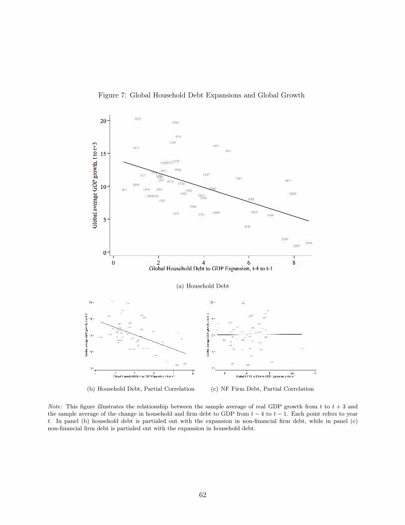
Figure 7: Global Household Debt Expansions and Global Growth
(a) Household Debt
(b) Household Debt, Partial Correlation (c) NF Firm Debt, Partial Correlation
Note: This figure illustrates the relationship between the sample average of real GDP growth from t to t + 3 andthe sample average of the change in household and firm debt to GDP from t− 4 to t− 1. Each point refers to yeart. In panel (b) household debt is partialed out with the expansion in non-financial firm debt, while in panel (c)non-financial firm debt is partialed out with the expansion in household debt.
62
Recommended