Homoclinic trajectories of non-autonomous maps
Thorsten Huls
Department of MathematicsBielefeld University
www.math.uni-bielefeld.de:~/huels
Thorsten Huls (Bielefeld University) ICDEA 2012 Homoclinic trajectories of non-autonomous maps
Non-autonomous dynamical systems
Spectral theory
Invariantfiber bundles
Hyperbolicity Asymptoticbehavior
Homoclinictrajectories
Non-autonomousbifurcations
Pullback attractors
Skew productflow
Thorsten Huls (Bielefeld University) ICDEA 2012 Homoclinic trajectories of non-autonomous maps
Non-autonomous dynamical systems
P. E. Kloeden and M. Rasmussen.Nonautonomous dynamical systems, volume 176 ofMathematical Surveys and Monographs.American Mathematical Society, Providence, RI, 2011.
C. Potzsche.Geometric theory of discrete nonautonomous dynamicalsystems, volume 2002 of Lecture Notes in Mathematics.Springer, Berlin, 2010.
M. Rasmussen.Attractivity and bifurcation for nonautonomous dynamicalsystems, volume 1907 of Lecture Notes in Mathematics.Springer, Berlin, 2007.
Thorsten Huls (Bielefeld University) ICDEA 2012 Homoclinic trajectories of non-autonomous maps
Outline
Homoclinic orbits in autonomoussystems
Thorsten Huls (Bielefeld University) ICDEA 2012 Homoclinic trajectories of non-autonomous maps
Homoclinic orbits in autonomous systems
Letf : k ! k be a smooth diffeomorphism,! be a hyperbolic fixed point, i.e. "(Df (!)) " {x # : |x| = 1} = $.Assume that stable and unstable manifold of ! intersect transversally.
!x0
x1x2
x!1
Ws(!)
Wu(!)
−1.5 −1 −0.5 0 0.5 1 1.5
−1
−0.5
0
0.5
1
DefinitionHomoclinic orbit: x = (xn)n" :
xn+1 = f(xn), n # , limn#±$
xn = !.
Thorsten Huls (Bielefeld University) ICDEA 2012 Homoclinic trajectories of non-autonomous maps
Homoclinic orbits in autonomous systems
RemarkThe dynamics near transversal homoclinic orbits is chaotic, cf. thecelebrated Smale-Sil’nikov-Birkhoff Theorem.
L. P. Sil’nikov.Existence of a countable set of periodic motions in a neighborhood of ahomoclinic curve.Dokl. Akad. Nauk SSSR, 172:298–301, 1967.Soviet Math. Dokl. 8 (1967), 102–106.
S. Smale.Differentiable dynamical systems.Bull. Amer. Math. Soc., 73:747–817, 1967.
K. J. Palmer.Shadowing in dynamical systems, volume 501 of Mathematics and itsApplications.Kluwer Academic Publishers, Dordrecht, 2000.
Thorsten Huls (Bielefeld University) ICDEA 2012 Homoclinic trajectories of non-autonomous maps
Approximation of homoclinic orbits in autonomous systems
Compute a finite orbit segment
xn! , . . . , xn+
by solving aboundary value problem.Simplest case: periodic boundary conditions:
x =
!"#xn!...
xn+
$%& , !(x) =
'xn+1 % f(xn), n = n!, . . . , n+ % 1
xn! % xn+
(.
Often successful: Rough initial guess for Newton’s method:
u0 = (!, . . . , !, g, !, . . . , !)T , e.g. g =
'1
%1
(in the Henon example.
Thorsten Huls (Bielefeld University) ICDEA 2012 Homoclinic trajectories of non-autonomous maps
Approximation of homoclinic orbits in autonomous systems
Compute a finite orbit segment
xn! , . . . , xn+
by solving aboundary value problem.Simplest case: periodic boundary conditions:
x =
!"#xn!...
xn+
$%& , !(x) =
'xn+1 % f(xn), n = n!, . . . , n+ % 1
xn! % xn+
(.
Alternative: Compute initial guess via approximations of stable andunstable manifolds.
R. K. Ghaziani, W. Govaerts, Y. A. Kuznetsov, and H. G. E. Meijer.Numerical continuation of connecting orbits of maps in MATLAB.J. Difference Equ. Appl., 15(8-9):849–875, 2009.
Thorsten Huls (Bielefeld University) ICDEA 2012 Homoclinic trajectories of non-autonomous maps
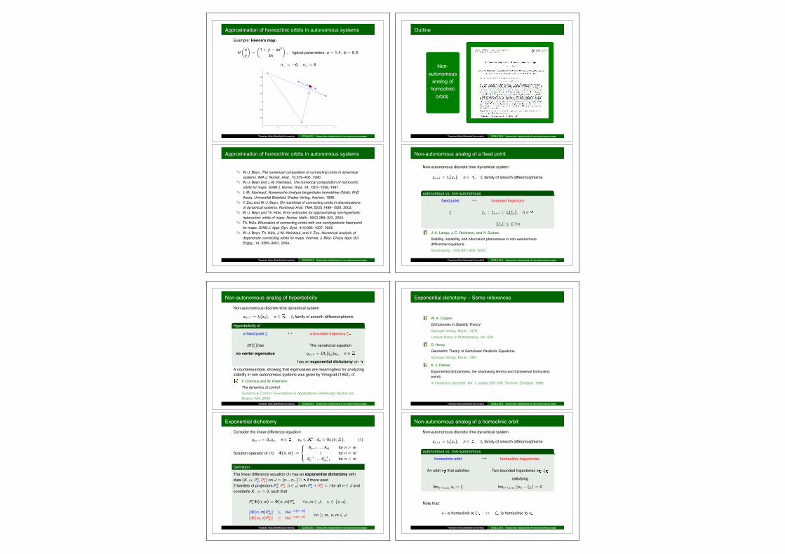
Approximation of homoclinic orbits in autonomous systems
Example: Henon’s map:
H'xy
(=
'1 + y % ax2
bx
(, typical parameters: a = 1.4, b = 0.3.
n! = %6, n+ = 6
−1 −0.5 0 0.5 1 1.5
−0.2
−0.1
0
0.1
0.2
0.3
Thorsten Huls (Bielefeld University) ICDEA 2012 Homoclinic trajectories of non-autonomous maps
Approximation of homoclinic orbits in autonomous systems
✎ W.-J. Beyn, The numerical computation of connecting orbits in dynamicalsystems. IMA J. Numer. Anal., 10,379–405, 1990.
✎ W.-J. Beyn and J.-M. Kleinkauf, The numerical computation of homoclinicorbits for maps. SIAM J. Numer. Anal., 34, 1207–1236, 1997.
✎ J.-M. Kleinkauf, Numerische Analyse tangentialer homokliner Orbits. PhDthesis, Universitat Bielefeld, Shaker Verlag, Aachen, 1998.
✎ Y. Zou and W.-J. Beyn, On manifolds of connecting orbits in discretizationsof dynamical systems. Nonlinear Anal. TMA, 52(5),1499–1520, 2003.
✎ W.-J. Beyn and Th. Huls. Error estimates for approximating non-hyperbolicheteroclinic orbits of maps. Numer. Math., 99(2):289–323, 2004.
✎ Th. Huls. Bifurcation of connecting orbits with one nonhyperbolic fixed pointfor maps. SIAM J. Appl. Dyn. Syst., 4(4):985–1007, 2005.
✎ W.-J. Beyn, Th. Huls, J.-M. Kleinkauf, and Y. Zou, Numerical analysis ofdegenerate connecting orbits for maps. Internat. J. Bifur. Chaos Appl. Sci.Engrg., 14, 3385–3407, 2004.
Thorsten Huls (Bielefeld University) ICDEA 2012 Homoclinic trajectories of non-autonomous maps
Outline
Non-autonomousanalog ofhomoclinicorbits
Thorsten Huls (Bielefeld University) ICDEA 2012 Homoclinic trajectories of non-autonomous maps
Non-autonomous analog of a fixed point
Non-autonomous discrete time dynamical system
xn+1 = fn(xn), n # , fn family of smooth diffeomorphisms
autonomous vs. non-autonomous
fixed point ↔ bounded trajectory
! ! : !n+1 = fn(!n), n #
&!n& ' C (nJ. A. Langa, J. C. Robinson, and A. Suarez.Stability, instability, and bifurcation phenomena in non-autonomousdifferential equations.Nonlinearity, 15(3):887–903, 2002.
Thorsten Huls (Bielefeld University) ICDEA 2012 Homoclinic trajectories of non-autonomous maps
Non-autonomous analog of hyperbolicity
Non-autonomous discrete time dynamical system
xn+1 = fn(xn), n # , fn family of smooth diffeomorphisms
Hyperbolicity of
a fixed point ! ↔ a bounded trajectory !
Df(!)has The variational equation
no center eigenvalue un+1 = Dfn(!n)un, n #has an exponential dichotomy on .
A counterexample, showing that eigenvalues are meaningless for analyzingstability in non-autonomous systems was given by Vinograd (1952), cf.
F. Colonius and W. Kliemann.The dynamics of control.Systems & Control: Foundations & Applications. Birkhauser Boston Inc.,Boston, MA, 2000.
Thorsten Huls (Bielefeld University) ICDEA 2012 Homoclinic trajectories of non-autonomous maps
Exponential dichotomy
Consider the linear difference equation
un+1 = Anun, n # , un # k , An # GL(k ; ). (1)
Solution operator of (1): "(n,m) :=
)*+
An!1 . . . Am for n > mI for n = m
A!1n . . . A!1
m!1 for n < m
DefinitionThe linear difference equation (1) has an exponential dichotomy withdata (K ,#,Ps
n ,Pun ) on J = [n!, n+] " if there exist
2 families of projectors Psn ,Pu
n , n # J, with Psn + Pu
n = I for all n # J andconstants K , # > 0, such that
P!n "(n,m) = "(n,m)P!
m (n,m # J, $ # {s, u},
&"(n,m)Psm& ' Ke!"(n!m)
&"(m, n)Pun& ' Ke!"(n!m) (n ) m, n,m # J.
Thorsten Huls (Bielefeld University) ICDEA 2012 Homoclinic trajectories of non-autonomous maps
Exponential dichotomy – Some references
W. A. Coppel.Dichotomies in Stability Theory.Springer-Verlag, Berlin, 1978.Lecture Notes in Mathematics, Vol. 629.
D. Henry.Geometric Theory of Semilinear Parabolic Equations.Springer-Verlag, Berlin, 1981.
K. J. Palmer.Exponential dichotomies, the shadowing lemma and transversal homoclinicpoints.In Dynamics reported, Vol. 1, pages 265–306. Teubner, Stuttgart, 1988.
Thorsten Huls (Bielefeld University) ICDEA 2012 Homoclinic trajectories of non-autonomous maps
Non-autonomous analog of a homoclinic orbit
Non-autonomous discrete time dynamical system
xn+1 = fn(xn), n # , fn family of smooth diffeomorphisms
autonomous vs. non-autonomous
homoclinic orbit ↔ homoclinic trajectories:
An orbit x that satisfies Two bounded trajectories x , !
satisfying
limn#±$ xn = ! limn#±$ &xn % !n& = 0
Note that:
x is homoclinic to ! * ! is homoclinic to x
Thorsten Huls (Bielefeld University) ICDEA 2012 Homoclinic trajectories of non-autonomous maps
Outline
Step 1
Approximation ofa bounded trajectory ! .
Step 2
Approximation ofa second trajectory xthat is homoclinic to ! .
Thorsten Huls (Bielefeld University) ICDEA 2012 Homoclinic trajectories of non-autonomous maps
Setup
xn+1 = fn(xn), n #fn is generated by a parameter-dependent map
fn = f(·,%n), % sequence of parameters.
Assumptions
❶ Smoothness: f # $( k + , k ), f(·,%) diffeomorphism for all% # .
❷ There exists % # such that!n+1 = f(!n, %n), n #
has a bounded solution ! .❸ The variational equation
un+1 = Dx f(!n, %n)un, n #has an exponential dichotomy on .
Thorsten Huls (Bielefeld University) ICDEA 2012 Homoclinic trajectories of non-autonomous maps
Approximation of bounded trajectories
Bounded trajectory !
Zero of the operator ! : X + ! X , defined as
!(! ,% ) :=,!n+1 % f(!n,%n)
-n" .
Space of bounded sequences on the discrete interval J
XJ :=
.uJ = (un)n"J # ( k)J : sup
n"J&un& < ,
/
Thorsten Huls (Bielefeld University) ICDEA 2012 Homoclinic trajectories of non-autonomous maps
Approximation of bounded trajectories
LemmaAssume❶ –❸.Then there exist two neighborhoods U(% ) and V(! ), such that
!(! ,% ) = 0
has for all % # U(% ) a unique solution ! # V(! ).
LemmaAssume❶ –❸.Then there exist two neighborhoods U(% ) and V(! ), such that
un+1 = Dxf(xn,%n)un, n #
has an exponential dichotomy on for any sequence x # V(! ),% # U(% ). The dichotomy constants are independent of the specificsequence x .
Thorsten Huls (Bielefeld University) ICDEA 2012 Homoclinic trajectories of non-autonomous maps
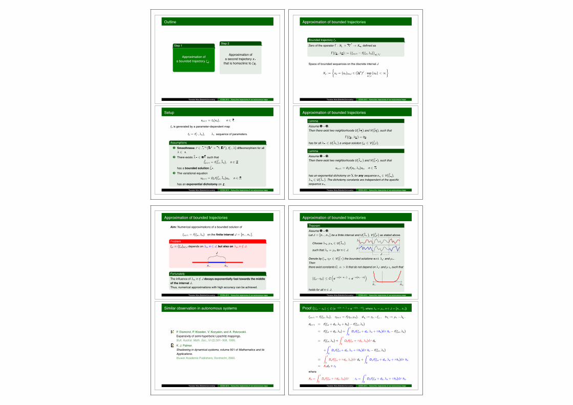
Approximation of bounded trajectories
Aim: Numerical approximations of a bounded solution of
!n+1 = f(!n,%n) on the finite interval J = [n!, n+].
Problem!J = (!n)n"J depends on %n, n # J, but also on %n, n /# J.
n! n+
J
FortunatelyThe influence of %n, n /# J decays exponentially fast towards the middleof the interval J.Thus, numerical approximations with high accuracy can be achieved.
Thorsten Huls (Bielefeld University) ICDEA 2012 Homoclinic trajectories of non-autonomous maps
Similar observation in autonomous systems
P. Diamond, P. Kloeden, V. Kozyakin, and A. Pokrovskii.Expansivity of semi-hyperbolic Lipschitz mappings.Bull. Austral. Math. Soc., 51(2):301–308, 1995.K. J. Palmer.Shadowing in dynamical systems, volume 501 of Mathematics and itsApplications.Kluwer Academic Publishers, Dordrecht, 2000.
Thorsten Huls (Bielefeld University) ICDEA 2012 Homoclinic trajectories of non-autonomous maps
Approximation of bounded trajectories
TheoremAssume❶ –❸.Let J = [n!, n+] be a finite interval and U(% ), V(! ) as stated above.
Choose % , µ # U(% )
such that %n = µn for n # J.µ
%
JDenote by ! , & # V(! ) the bounded solutions w.r.t. % and µ .Thenthere exist constants C, # > 0 that do not depend on % and µ , such that
&!n%&n& ' C0e!"(n!n!) + e!"(n+!n)
1
n! n+
holds for all n # J.Thorsten Huls (Bielefeld University) ICDEA 2012 Homoclinic trajectories of non-autonomous maps
Proof (&!n % &n& ' C,e!!(n!n!) + e!!(n+!n)
-, where %n = µn, n # J = [n!, n+])
!n+1 = f(!n,%n), &n+1 = f(&n, µn), d := & %! , h := µ %% .
dn+1 = f(!n + dn,%n + hn) % f(!n,%n)
= f(!n + dn,%n) +
2 1
0D#f(!n + dn,%n + 'hn)d' hn % f(!n,%n)
= f(!n,%n) +
2 1
0Dx f(!n + 'dn,%n)d' dn
+
2 1
0D#f(!n + dn,%n + 'hn)d' hn % f(!n,%n)
=
2 1
0Dx f(!n + 'dn,%n)d' dn +
2 1
0D#f(!n + dn,%n + 'hn)d' hn
= Andn + rnwhere
An =
2 1
0Dx f(!n + 'dn,%n)d' rn =
2 1
0D#f(!n + dn,%n + 'hn)d' hn.
Thorsten Huls (Bielefeld University) ICDEA 2012 Homoclinic trajectories of non-autonomous maps
Proof (&!n % &n& ' C,e!!(n!n!) + e!!(n+!n)
-, where %n = µn, n # J = [n!, n+])
An =
2 1
0Dx f(!n + 'dn,%n)d' rn =
2 1
0D#f(!n + dn,%n + 'hn)d' hn
By assumption❸
un+1 = Dxf(!n, %n)un, n #
has an exponential dichotomy on .
Due to the Roughness-Theorem and our construction of neighborhoods,
un+1 = Anun, n #
has an exponential dichotomy on with data (K ,#,Psn ,Pu
n ).
Solution operator: "(n,m), i.e. un = "(n,m)umThorsten Huls (Bielefeld University) ICDEA 2012 Homoclinic trajectories of non-autonomous maps
Proof (&!n % &n& ' C,e!!(n!n!) + e!!(n+!n)
-, where %n = µn, n # J = [n!, n+])
An =
2 1
0Dx f(!n + 'dn,%n)d' rn =
2 1
0D#f(!n + dn,%n + 'hn)d' hn
Unique bounded solution of un+1 = Anun + rn on :
un =3
m"G(n,m + 1)rm,
where G is Green’s function, defined as
G(n,m) =
."(n,m)Ps
m, n ) m,%"(n,m)Pu
m, n < m.
Estimates:
&G(n,m)& = &"(n,m)Psm& ' Ke!"(n!m), for n ) m,
&G(n,m)& = &"(n,m)Pum& ' Ke!"(m!n), for n < m.
Thorsten Huls (Bielefeld University) ICDEA 2012 Homoclinic trajectories of non-autonomous maps
Proof (&!n % &n& ' C,e!!(n!n!) + e!!(n+!n)
-, where %n = µn, n # J = [n!, n+])
An =
2 1
0Dx f(!n + 'dn,%n)d' rn =
2 1
0D#f(!n + dn,%n + 'hn)d' hn
un =3
m"G(n,m+1)rm, &G(n,m)& =
.&"(n,m)Ps
m& ' Ke!!(n!m), n ) m,
&"(n,m)Pum& ' Ke!!(m!n), n < m.
&un& 'n!!13
m=!$&G(n,m + 1)rm& +
$3
m=n++1
&G(n,m + 1)rm&
'n!!13
m=!$RKe!"(n!m!1) +
$3
m=n++1
RKe!"(m+1!n)
=RK
1 % e!"
0e!"(n!n!) + e!"(n+!n+2)
1, n # J.
Thorsten Huls (Bielefeld University) ICDEA 2012 Homoclinic trajectories of non-autonomous maps
Proof (&!n % &n& ' C,e!!(n!n!) + e!!(n+!n)
-, where %n = µn, n # J = [n!, n+])
An =
2 1
0Dx f(!n + 'dn,%n)d' rn =
2 1
0D#f(!n + dn,%n + 'hn)d' hn
un+1 = Anun + rn, n # (2)
&un& ' RK1 % e!"
0e!"(n!n!) + e!"(n+!n+2)
1, n # J.
d = ! % & is the unique bounded solution of (2), thus
&dn& = &!n % &n& ' C0e!"(n!n!) + e!"(n+!n)
1, n # J.
Thorsten Huls (Bielefeld University) ICDEA 2012 Homoclinic trajectories of non-autonomous maps
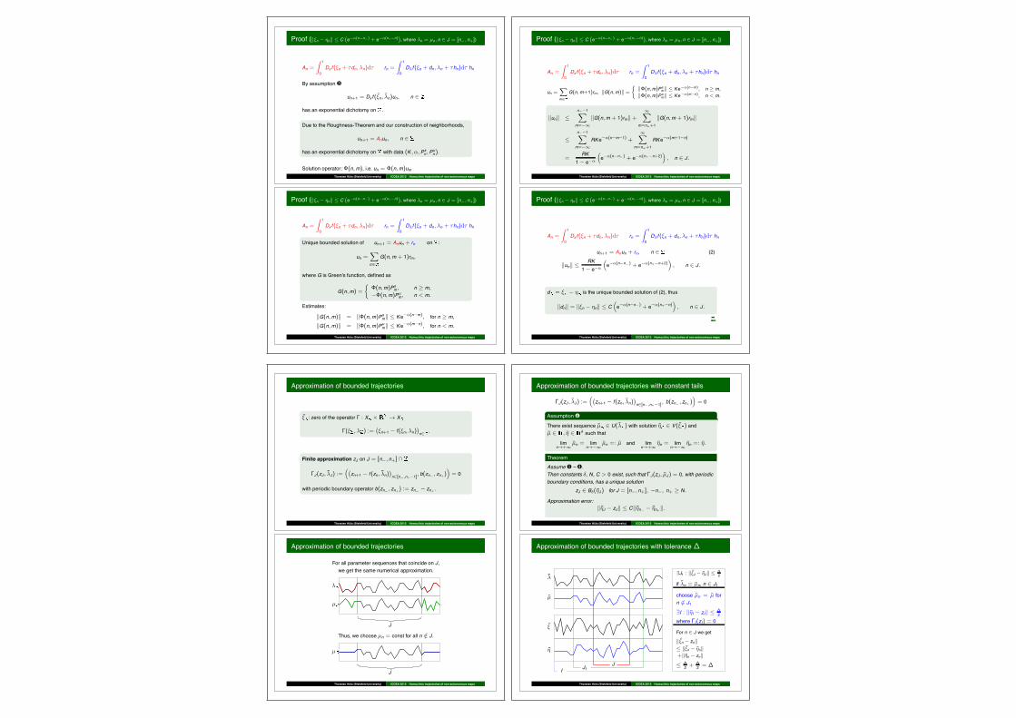
Approximation of bounded trajectories
! : zero of the operator ! : X + ! X
!(! ,% ) :=,!n+1 % f(!n,%n)
-n" .
Finite approximation zJ on J = [n!, n+] "
!J(zJ , %J) :=0,zn+1 % f(zn, %n)
-n"[n!,n+!1], b(zn! , zn+)
1= 0
with periodic boundary operator b(zn! , zn+) := zn! % zn+ .
Thorsten Huls (Bielefeld University) ICDEA 2012 Homoclinic trajectories of non-autonomous maps
Approximation of bounded trajectories
For all parameter sequences that coincide on J,we get the same numerical approximation.
%
µ
J
Thus, we choose µn = const for all n /# J.
µ
J
Thorsten Huls (Bielefeld University) ICDEA 2012 Homoclinic trajectories of non-autonomous maps
Approximation of bounded trajectories with constant tails
!J(zJ , %J) :=0,zn+1 % f(zn, %n)
-n"[n!,n+!1], b(zn! , zn+)
1= 0
Assumption❹
There exist sequence µ # U(% ) with solution & # V(! ) andµ # , & # k such that
limn#+$
µn = limn#!$
µn =: µ and limn#+$
&n = limn#!$
&n =: &.
TheoremAssume❶ –❹.Then constants (, N, C > 0 exist, such that !J(zJ , µJ) = 0, with periodicboundary conditions, has a unique solution
zJ # B$(&J) for J = [n!, n+], %n!, n+ ) N.
Approximation error:&&J % zJ& ' C&&n! % &n+&.
Thorsten Huls (Bielefeld University) ICDEA 2012 Homoclinic trajectories of non-autonomous maps
Approximation of bounded trajectories with tolerance !
JJ1I
%
µ
!
&
-J1 : &!J % &J& ' !2
if %n = µn, n # J1
choose µn = µ forn /# J1-I : &&I % zI& ' !
2where !I(zI) = 0
For n # J we get
&!n % zn&' &!n % &n&+&&n % zn&' !
2 + !2 = #
Thorsten Huls (Bielefeld University) ICDEA 2012 Homoclinic trajectories of non-autonomous maps
Outline
Numerical experiments:
Computation of bounded trajectories
Thorsten Huls (Bielefeld University) ICDEA 2012 Homoclinic trajectories of non-autonomous maps
Example: Computation of bounded trajectories
Henon’s map
x .! h(x,%, b) =
'1 + x2 % %x21
bx1
(
Fix b = 0.3 and choose % # [1, 2] at random.
Non-autonomous difference equation
xn+1 = h(xn,%n, b), n # .
M. Henon.A two-dimensional mapping with a strange attractor.Comm. Math. Phys., 50(1):69–77, 1976.
Thorsten Huls (Bielefeld University) ICDEA 2012 Homoclinic trajectories of non-autonomous maps
Example: Computation of bounded trajectories
Solutions of !J = 0 on J = [%40, 40] for two sequences %J that coincideon [-20,20].
−40 −30 −20 −10 0 10 20 30 400.5
0.6
0.7
0.8
−40 −30 −20 −10 0 10 20 30 401
0
2
xn
%n
n
n
Thorsten Huls (Bielefeld University) ICDEA 2012 Homoclinic trajectories of non-autonomous maps
Example: Computation of bounded trajectories on J = [%150, 150]
Given a sequence %J # [1, 2]J with corresponding solution !J .Let µJ # [1, 2]J such that %n = µn for n # [%100, 100] and solution &J .
−150 −100 −50 0 50 100 15010−16
10−14
10−12
10−10
10−8
10−6
10−4
10−2
100
dn
n! n+n! n+
dn = &!n % &n&, n # J for10 different sequences µJ .
Interval where dn ' #
n! =4n! + | log!|
"!
5,
n+ =6n+ % | log!|
"+
7,
#± dichotomy constants,
# = 10!16.
Thorsten Huls (Bielefeld University) ICDEA 2012 Homoclinic trajectories of non-autonomous maps
Example: Computation of bounded trajectories on J = [%20, 20]
Choose a buffer interval [n!, n+] such that we get an accurateapproximation on [%20, 20]:
n! =
8n! % | log#|
#!
9= %40 and n+ =
:n+ +
| log#|#+
;= 74.
−40 −20 0 20 40 600.45
0.5
0.55
0.6
0.65
0.7
0.75
0.8
−20 −15 −10 −5 0 5 10 15 200.45
0.5
0.55
0.6
0.65
0.7
0.75
0.8
x1x1
n!n! n+n+n! n+
Thorsten Huls (Bielefeld University) ICDEA 2012 Homoclinic trajectories of non-autonomous maps
Outline
Step 1 (done)
Approximation ofa bounded trajectory ! .
Step 2
Approximation ofa second trajectory xthat is homoclinic to ! .
Thorsten Huls (Bielefeld University) ICDEA 2012 Homoclinic trajectories of non-autonomous maps
Homoclinic trajectories
Assumptions
❺ Let % as in ❷. A solution x of
xn+1 = f(xn, %n), n #
exists, that is homoclinic to ! and non-trivial, i.e. x /= ! .❻ The trajectory x is transversal, i.e.
un+1 = Dxf(xn, %n)un, n # for u # X 01 u = 0.
LemmaAssume❶ –❻. Then the difference equation
un+1 = Dx f(xn, %n)un, n # .
has an exponential dichotomy on .
Thorsten Huls (Bielefeld University) ICDEA 2012 Homoclinic trajectories of non-autonomous maps
Homoclinic trajectories
x is homoclinic to !
if and only if
y defined as
yn = xn % !n
is a homoclinic orbit of
yn+1 = g(yn, %n) := f(yn + !n, %n) % !n+1 n #w.r.t. the fixed point 0.
The f and g-system are topologically equivalent due to the kinematictransformation, cf.
B. Aulbach and T. Wanner.Invariant foliations and decoupling of non-autonomous difference equations.J. Difference Equ. Appl., 9(5):459–472, 2003.
Thorsten Huls (Bielefeld University) ICDEA 2012 Homoclinic trajectories of non-autonomous maps
Approximation of homoclinic trajectories
gn(y) := f(y + !n, %n) % !n+1, yn+1 = gn(yn), gn(0) = 0, n # .
Approximation
!J(yJ) :=0,yn+1 % gn(yn)
-n"[n!,n+!1], yn! % yn+
1= 0
with periodic boundary conditions.Assumptions❼ Denote by Ps
n ,Pun the dichotomy projectors of
un+1 = Df(!n, %n)un, n # .
Assume for all sufficiently large %n!, n+:
!(R(Psn!),R(Pu
n+)) > ", for a 0 < " <
)
2.
Thorsten Huls (Bielefeld University) ICDEA 2012 Homoclinic trajectories of non-autonomous maps
Approximation of homoclinic trajectories
gn(y) := f(y + !n, %n) % !n+1, yn+1 = gn(yn), gn(0) = 0, n # .
TheoremAssume❶ –❽.Then there exist constants (, N, C > 0, such that!J(yJ) = 0, with projection boundary conditions, has a unique solution
yJ # B$(yJ) for all J = [n!, n+],
where %n!, n+ ) N.Approximation error: &yJ % yJ& ' C&yn! % yn+&.
Th. Huls.Homoclinic orbits of non-autonomous maps and their approximation.J. Difference Equ. Appl., 12(11):1103–1126, 2006.
Thorsten Huls (Bielefeld University) ICDEA 2012 Homoclinic trajectories of non-autonomous maps
Outline
Numerical experiments:
Computation of homoclinic trajectories(a) for the Henon system,(b) for a predator-prey model.
Thorsten Huls (Bielefeld University) ICDEA 2012 Homoclinic trajectories of non-autonomous maps
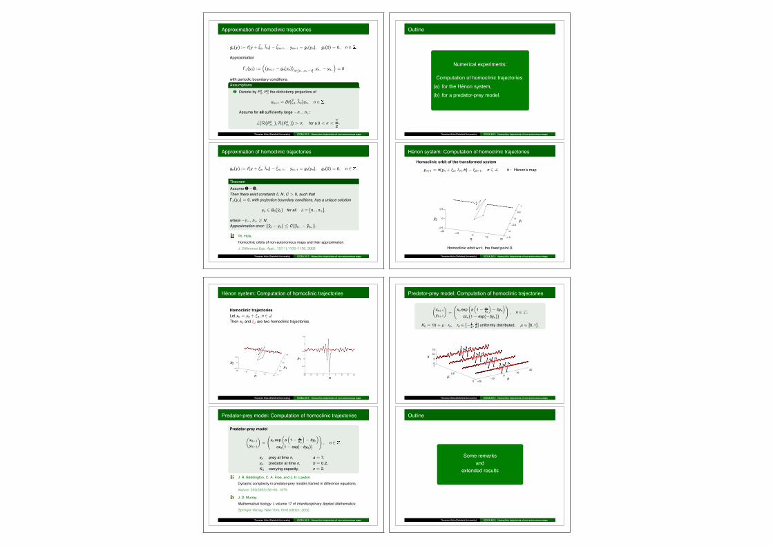
Henon system: Computation of homoclinic trajectories
Homoclinic orbit of the transformed system
yn+1 = h(yn + !n,%n, b) % !n+1, n # J, h : Henon’s map
−20−10
010
20 −1.5
−1
−0.5
0
0.5
1
−0.5
0
0.5
y1y2
n
Homoclinic orbit w.r.t. the fixed point 0.
Thorsten Huls (Bielefeld University) ICDEA 2012 Homoclinic trajectories of non-autonomous maps
Henon system: Computation of homoclinic trajectories
Homoclinic trajectoriesLet xn = yn + !n, n # J.Then xJ and !J are two homoclinic trajectories.
−20−10
010
20 −1
−0.5
0
0.5
1
1.5
−0.5
0
0.5
−20 −15 −10 −5 0 5 10 15 20−1
−0.5
0
0.5
1
1.5
x1
x1x2
n n
Thorsten Huls (Bielefeld University) ICDEA 2012 Homoclinic trajectories of non-autonomous maps
Predator-prey model: Computation of homoclinic trajectories
Predator-prey model
'xn+1yn+1
(=
<xn exp
0a01 % xn
Kn
1% byn
1
cxn,1 % exp(%byn)
-=
, n # .
xn prey at time n,yn predator at time n,Kn carrying capacity,
a = 7,b = 0.2,c = 2.
J. R. Beddington, C. A. Free, and J. H. Lawton.Dynamic complexity in predator-prey models framed in difference equations.Nature, 255(5503):58–60, 1975.
J. D. Murray.Mathematical biology. I, volume 17 of Interdisciplinary Applied Mathematics.Springer-Verlag, New York, third edition, 2002.
Thorsten Huls (Bielefeld University) ICDEA 2012 Homoclinic trajectories of non-autonomous maps
Predator-prey model: Computation of homoclinic trajectories
'xn+1yn+1
(=
<xn exp
0a01 % xn
Kn
1% byn
1
cxn,1 % exp(%byn)
-=
, n # .
Kn = 10 + µ · rn, rn # [% 12 ,
12 ] uniformly distributed, µ # [0, 1].
−20−10
010
20
0
0.5
10
5
10
15
x
nµ
Thorsten Huls (Bielefeld University) ICDEA 2012 Homoclinic trajectories of non-autonomous maps
Outline
Some remarksand
extended results
Thorsten Huls (Bielefeld University) ICDEA 2012 Homoclinic trajectories of non-autonomous maps
Remarks: Invariant fiber bundles
Stable and unstable fiber bundles are the non-autonomous generalizati-on of stable and unstable manifolds:$ : solution operator of xn+1 = fn(xn),
Ss0(! ) =>x # k : lim
m#$&$(m, 0)(x) % !m& = 0
?,
Su0(! ) =
.x # k : lim
m#!$&$(m, 0)(x) % !m& = 0
/.
Approximation results:C. Potzsche and M. Rasmussen.Taylor approximation of invariant fiber bundles for non-autonomousdifference equations.Nonlinear Anal., 60(7):1303–1330, 2005.
Let x be a homoclinic trajectory w.r.t. ! . Then
x0 # Ss0(! ) " Su0 (! ).
Thorsten Huls (Bielefeld University) ICDEA 2012 Homoclinic trajectories of non-autonomous maps
Heteroclinic trajectories
Autonomous world: Heteroclinic orbit.Let !+ and !! two fixed points.A trajectory x is heteroclinic w.r.t. !±, if
limn#!$
xn = !!, limn#$
xn = !+.
Non-autonomous analog: Heteroclinic trajectories.Let !! be a trajectory that is bounded in backward time, andlet !+ be a trajectory that is bounded in forward time.A trajectory x is heteroclinic w.r.t. !±, if
limn#!$
&xn % !!n & = 0, lim
n#$&xn % !+
n & = 0.
Th. Huls and Y. Zou.On computing heteroclinic trajectories of non-autonomous maps.Discrete Contin. Dyn. Syst. Ser. B, 17(1):79–99, 2012.
Thorsten Huls (Bielefeld University) ICDEA 2012 Homoclinic trajectories of non-autonomous maps
Heteroclinic trajectories
%s0
%u0
x
!!!
!++
Ss0(x )
Su0(x )
Problem: Families of semi-bounded trajectories exist.Separate one semi-bounded trajectory by posing an initial condition.
Thorsten Huls (Bielefeld University) ICDEA 2012 Homoclinic trajectories of non-autonomous maps
Heteroclinic trajectories
One achieves accurate approximations of semi-bounded and heteroclinictrajectories, by solving appropriate boundary value problems.
n! n+
n1! n1+n2! n2+
approximation of x
approximation of !! approximation of !+
Boundary operator:
b(xn! , xn+) =
'YT
!(xn! % !!n!)
YT+(xn+ % !!
n+!)
(,
Y!: base of R(Pun!)%, Y+: base of R(Ps
n+)%.
Thorsten Huls (Bielefeld University) ICDEA 2012 Homoclinic trajectories of non-autonomous maps
Computation of dichotomy projectors
Fix N # and compute PsN as follows:
For each i = 1, . . . , k solve for n #
uin+1 = Anuin + (n,N!1ei , n # , An = Dfn(!±n )
ei : i-th unit vector, ( : Kronecker symbol.
Unique bounded solution for n # :
uin = G(n,N)ei , G(n,N) =
."(n,N)Ps
N , n ) N,%"(n,N)Pu
N , n < N.
ThusuiN = G(N,N)ei = Ps
Nei .
ThereforePsN =
,u1N u2N . . . ukN
-.
Finite approximations can be achieved since errors decay exponentiallyfast towards the midpoint.
Thorsten Huls (Bielefeld University) ICDEA 2012 Homoclinic trajectories of non-autonomous maps
Computation of dichotomy projectors
Error estimates for approximate dichotomy projectors:Th. Huls.Numerical computation of dichotomy rates and projectors in discrete time.Discrete Contin. Dyn. Syst. Ser. B, 12(1):109–131, 2009.
Extended results:Th. Huls.Computing Sacker-Sell spectra in discrete time dynamical systems.SIAM J. Numer. Anal., 48(6):2043–2064, 2010.
Thorsten Huls (Bielefeld University) ICDEA 2012 Homoclinic trajectories of non-autonomous maps
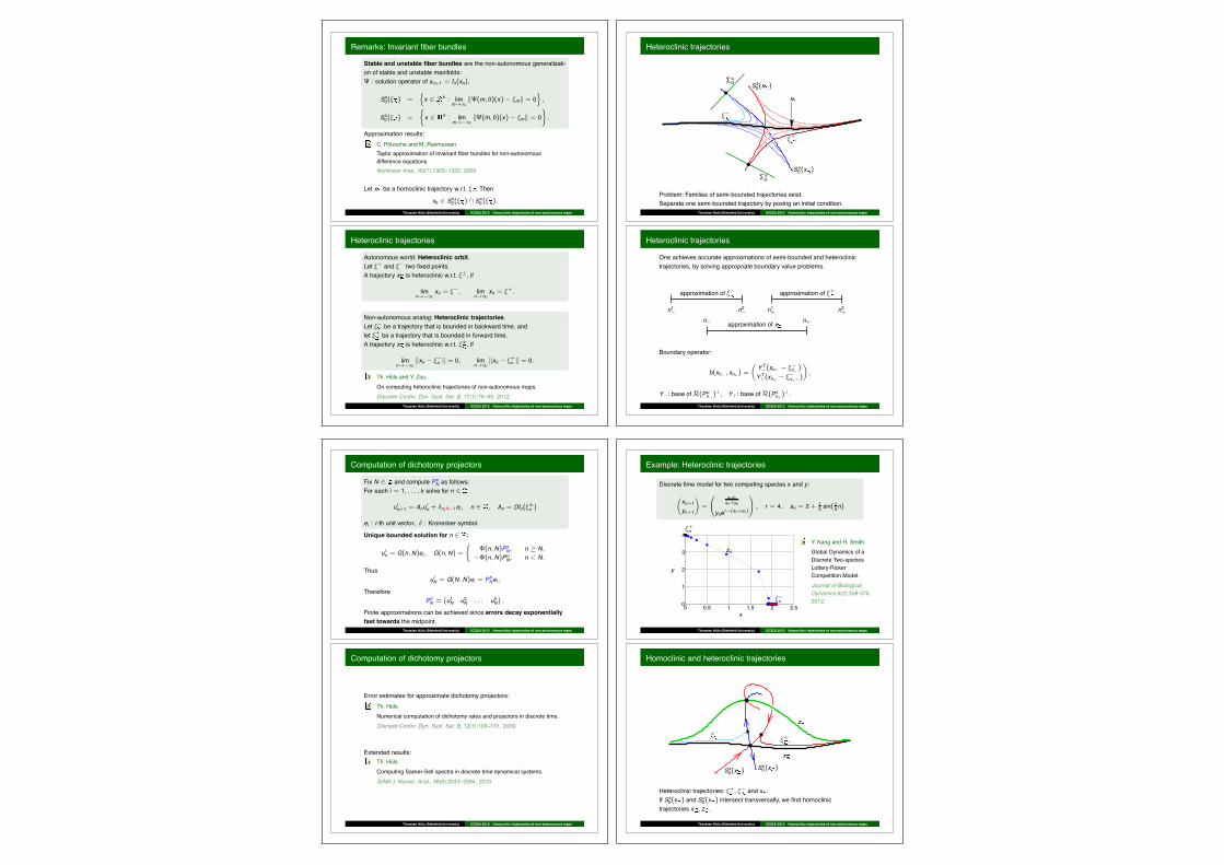
Example: Heteroclinic trajectories
Discrete time model for two competing species x and y :
'xn+1yn+1
(=
< snxnxn+yn
yner!(xn+yn)
=, r = 4, sn = 2 + 1
5 sin(15n)
0 0.5 1 1.5 2 2.50
1
2
3
4
x
y
!!n
!+n
znY. Kang and H. Smith.Global Dynamics of aDiscrete Two-speciesLottery-RickerCompetition Model.Journal of BiologicalDynamics 6(2):358-376,2012.
Thorsten Huls (Bielefeld University) ICDEA 2012 Homoclinic trajectories of non-autonomous maps
Homoclinic and heteroclinic trajectories
z
!!!
!++
x
Ss0(x ) Su0(x )
Heteroclinic trajectories: !+, !! and x .If Ss0(x ) and Su0(x ) intersect transversally, we find homoclinictrajectories x , z .
Thorsten Huls (Bielefeld University) ICDEA 2012 Homoclinic trajectories of non-autonomous maps

Conclusion
We derive approximation results for homoclinic (and heteroclinic)trajectories via boundary value problems.Justification: Due to our hyperbolicity assumptions, errors onfinite intervals decay exponentially fast toward the midpoint.One can verify these hyperbolicity assumption, using techniques thathave been introduced, for example, in:
L. Dieci, C. Elia, and E. Van Vleck.Exponential dichotomy on the real line: SVD and QR methods.J. Differential Equations, 248(2):287–308, 2010.Th. Huls.Computing Sacker-Sell spectra in discrete time dynamical systems.SIAM J. Numer. Anal., 48(6):2043–2064, 2010.
Thorsten Huls (Bielefeld University) ICDEA 2012 Homoclinic trajectories of non-autonomous maps
Conclusion
The exponential decay of error enables accurate computation ofcovariant vectors:
G. Froyland, Th. Huls, G.P. Morriss and Th.M. Watson.Computing covariant vectors, Lyapunov vectors, Oseledets vectors,and dichotomy projectors: a comparative numerical study.arXiv:1204.0871, 2012.
Thorsten Huls (Bielefeld University) ICDEA 2012 Homoclinic trajectories of non-autonomous maps
Recommended