1
Sensors and Materials vol. 16, in press (2004)
Higher-Order Statistics for Fluctuation-Enhanced Gas-Sensing
J. M. Smulko* and L. B. Kish
Department of Electrical Engineering, Texas A&M University, College Station, TX 77843-3128,
USA
e-mails: [email protected] and [email protected]
*Also at: Gdansk Univ. of Technology, WETiI, ul. G. Narutowicza 11/12 80-952 Gdansk, Poland

2
ABSTRACT
The stochastic component of a chemical sensor signal contains valuable information that can be
visualized not only by spectral analysis but also by methods of higher-order statistics (HOS). The
analysis of HOS enables the extraction of non-conventional features and may lead to significant
improvements in selectivity and sensitivity. We pay particular attention to the bispectrum that
characterizes the non-Gaussian component and detects non-stationarity in analyzed noise. The
results suggest that the bispectrum can be applied for gas recognition. The analysis of bispectra and
the reproducibility statistics of skewness and kurtosis indicate that the measured time records were
stationary.
KEYWORDS
gas detection, gas recognition, stochastic processes, sensor signal processing, pattern generation
3
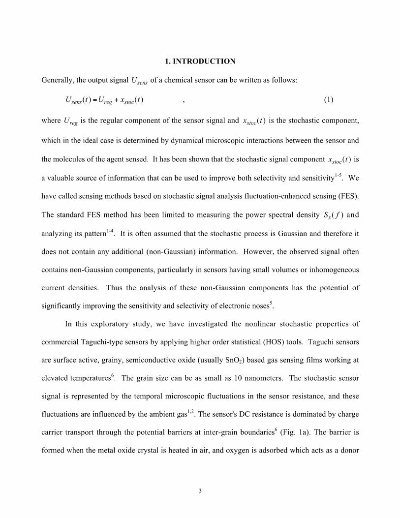
1. INTRODUCTION
Generally, the output signal
€
Usens of a chemical sensor can be written as follows:
€
Usens(t ) =Ureg + xstoc(t ) , (1)
where
€
Ureg is the regular component of the sensor signal and
€
xstoc(t ) is the stochastic component,
which in the ideal case is determined by dynamical microscopic interactions between the sensor and
the molecules of the agent sensed. It has been shown that the stochastic signal component
€
xstoc(t ) is
a valuable source of information that can be used to improve both selectivity and sensitivity1-5. We
have called sensing methods based on stochastic signal analysis fluctuation-enhanced sensing (FES).
The standard FES method has been limited to measuring the power spectral density
€
Sx( f ) and
analyzing its pattern1-4. It is often assumed that the stochastic process is Gaussian and therefore it
does not contain any additional (non-Gaussian) information. However, the observed signal often
contains non-Gaussian components, particularly in sensors having small volumes or inhomogeneous
current densities. Thus the analysis of these non-Gaussian components has the potential of
significantly improving the sensitivity and selectivity of electronic noses5.
In this exploratory study, we have investigated the nonlinear stochastic properties of
commercial Taguchi-type sensors by applying higher order statistical (HOS) tools. Taguchi sensors
are surface active, grainy, semiconductive oxide (usually SnO2) based gas sensing films working at
elevated temperatures6. The grain size can be as small as 10 nanometers. The stochastic sensor
signal is represented by the temporal microscopic fluctuations in the sensor resistance, and these
fluctuations are influenced by the ambient gas1,2. The sensor's DC resistance is dominated by charge
carrier transport through the potential barriers at inter-grain boundaries6 (Fig. 1a). The barrier is
formed when the metal oxide crystal is heated in air, and oxygen is adsorbed which acts as a donor
4
due to its negative charge. The barrier height is reduced6 when the concentration of oxygen ions
decreases in the presence of a reducing gas (Fig. 1b). As a result, the DC resistance decreases. The
gas-induced stochastic resistance fluctuations are caused by the fluctuations in the local oxygen
concentration at the grain boundary junctions1. These concentration fluctuations have two different
origins3 :
♦ The stochastic nature of the absorption-desorption process, which has also been observed in
surface acoustic wave (SAW) devices, is controlled by the adhesion energy of the gas
molecules at the surface.
♦ The stochastic nature of surface diffusion process (random walk) which is characterized by
the activation energy of surface diffusion.
These two microphysical stochastic processes are always present; however, usually one is the
dominant3. The actual situation is determined by the geometry, the activation and adhesion energies,
and the time scale (frequency range) of the measurement.
In this paper, we exploit the information captured in the HOS of the recorded stochastic
signal of commercial Taguchi sensors.

5
2. METHOD, SETUP AND SENSORS
2.1 Higher-Order Statistical (HOS) Methods
A stationary stochastic signal
€
x(t ) is characterized separately by its power spectral density
(PSD) and amplitude density. Usually, it is assumed that the observed noise is a Gaussian stochastic
process, implying a Gaussian amplitude density, in which case the PSD characterizes completely its
statistical properties. However, non-Gaussian stochastic processes are often present, and they play
an important role in various semiconductor devices7-9. For example, in the presence of random
telegraph noise, the observed deviation from a Gaussian distribution is used for reliability
predictions for semiconductor devices9.
Let us suppose that the
€
x(t ) sensor signal is sampled and recorded as a time series
€
x(n).
Simple measures of deviations10 from Gaussian distribution are skewness,
€
γ3, and kurtosis,
€
γ4 .
These parameters are computed for a discrete-time random process
€
x(n) having standard deviation
€
σ x by the following relations:
€
γ3 =1
σx3
E x(n)− E x(n)[ ]( )3
(2)
€
γ4 =1
σ x4
E x(n) − E x(n)[ ]( )4
− 3 , (3)
where E[] denotes an average. The skewness describes the degree of symmetry and the kurtosis

6
measures the relative peakedness of the distribution. Both measures are equal to zero for a Gaussian
process.
An important tool to investigate the non-Gaussian component of the stochastic sensor signal
is the bispectrum10-11. The bispectrum function is the second-order Fourier transform of the
third–order cummulant11:
€
S3x( f1, f2 ) = C3x(k ,l )e− j2πf1ke− j2πf2l
l=−∞
∞
∑k=−∞
∞
∑ (4)
where
€
C3x(k ,l ) = E[x(n)x(n + k )x(n + l )] is the third-order cummulant of the zero-mean process
€
x(n). The bispectrum is a two-dimensional complex function. Usually, its absolute value is
analyzed, which is a three-dimensional landscape. The bispectrum function is equal to zero for
processes with zero skewness, i.e. for Gaussian processes. The bispectrum of two statistically
independent random processes equals the sum of the bispectra of the individual random processes. It
is an important property of bispectra that Gaussian components in the recorded stochastic process
are eliminated and only the non-Gaussian component are seen11.
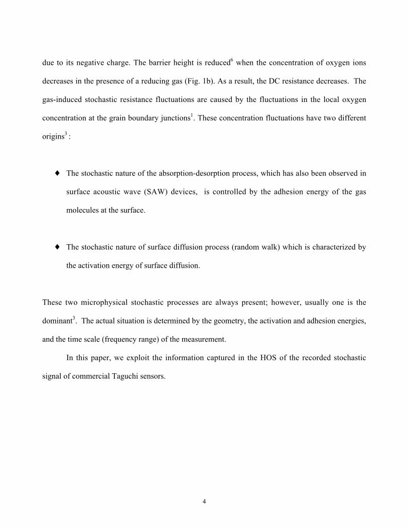
The above definition of the bispectrum function yields axial symmetries for stationary
random signals (Fig. 2), where each section between the symmetry axes characterizes the entire
function. The lack of any of these symmetries indicates that the analyzed process is not stationary.
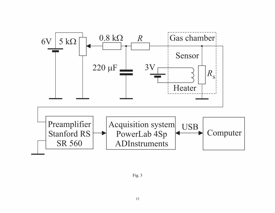
2.2 The Measurement Setup
The experimental setup (Fig. 3) consists of a gas mixer, a stainless steel sensor chamber, a Stanford
Instruments preamplifier, an ADInstruments PowerLab Data Acquisition system and a personal
computer. The passive current generator driving the sensor film (two-contact arrangement) and the

7
preamplifier were battery powered.
The flow of the gas mixture through the sensor chamber was controlled and held constant.
For the exploratory study of bispectra-based responses, we have measured the following four gas
mixtures:
• Synthetic air (flow 0.165 l/min);
• Ethanol (70 ppm) in synthetic air (flow 0.215 l/min);
• Hydrogen (380 ppm) in synthetic air (flow 0.265 l/min);
• Alcohol fumes (saturated ethanol vapor in closed sensor chamber).
The data were collected at sampling frequencies fs=20 kHz or fs=100 Hz. The noise
bandwidth was appropriately limited by the preamplifier filter to avoid aliasing effects. The load
resistance R was chosen to have approximately the same value as the sensor resistance Rs.
2.3 The Sensors
Two commercially available Taguchi type gas sensors were investigated: RS 286-636
(designed for the detection of carbon monoxide) and RS 286-642 (designed for the detection of
nitrogen oxide).
3. RESULTS AND DISCUSSION
We found that the properties of measured stochastic resistance fluctuations were
characteristic of the gas mixture used in the experiment. The normalized power spectra
€
f Sx( f ) /UDC2 of ethanol (70 ppm), hydrogen (380 ppm) and synthetic air are shown in Fig. 4,
recorded with a sampling frequency fs=20 kHz and 400,000 data points. The normalized power
spectra show distinctive characteristics (Fig. 4). At the same time, the amplitude density was nearly

8
Gaussian (Fig. 5). Stronger deviations from normal distribution were observed only at relatively
high amplitudes in ethanol with the carbon monoxide sensor (Fig. 5a). In conclusion, the measured
fluctuations were weakly non-Gaussian, which is a plausible result because of the large size of these
sensors and due the central limit theorem.
To explore this week non-Gaussianity, we analyzed the bispectra of these records. At a
sampling frequency of 20 kHz, the measured bispectra were non-zero only around the point f1=f2=0.
This fact indicates that the most important non-Gaussian information is located at low frequencies
and their detailed study required a lower sampling frequency.
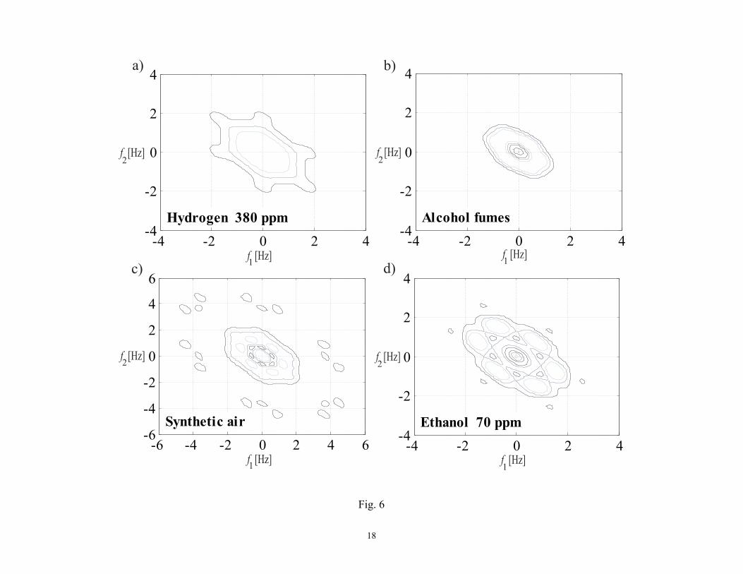
Therefore, we ran new measurements at a sampling frequency fs = 100 Hz (200-times lower)
to see the characteristic features at lower frequencies. For convenience, in Fig. 6 we plot the cross-
level contour-plot of the absolute value of the bispectra11. Throughout this paper, we will refer to
this plot as a bispectrum in accordance with existing fashion in the literature. The bispectra of the
four gas mixtures (Fig. 6) show distinct features in each case. The characteristic differences
between these bispectra provide significantly more information, a kind of "chemical fingerprint".
This information is independent of the power spectra (Fig. 4). Thus the bispectrum is a powerful
additional tool to identify various gas mixtures using a single sensor. It is important to emphasize
that this goal cannot be achieved when the sensor is used in the classical way to analyze only the
mean resistance because that provides only a single number instead of a rich pattern.
The axial symmetries of the obtained bispectrum functions obtained (Fig. 6) satisfy the
symmetry condition for a stationary time series. This indicates that the observed non-zero
bispectrum is not due to hidden non-stationary processes in the stochastic component of the sensor
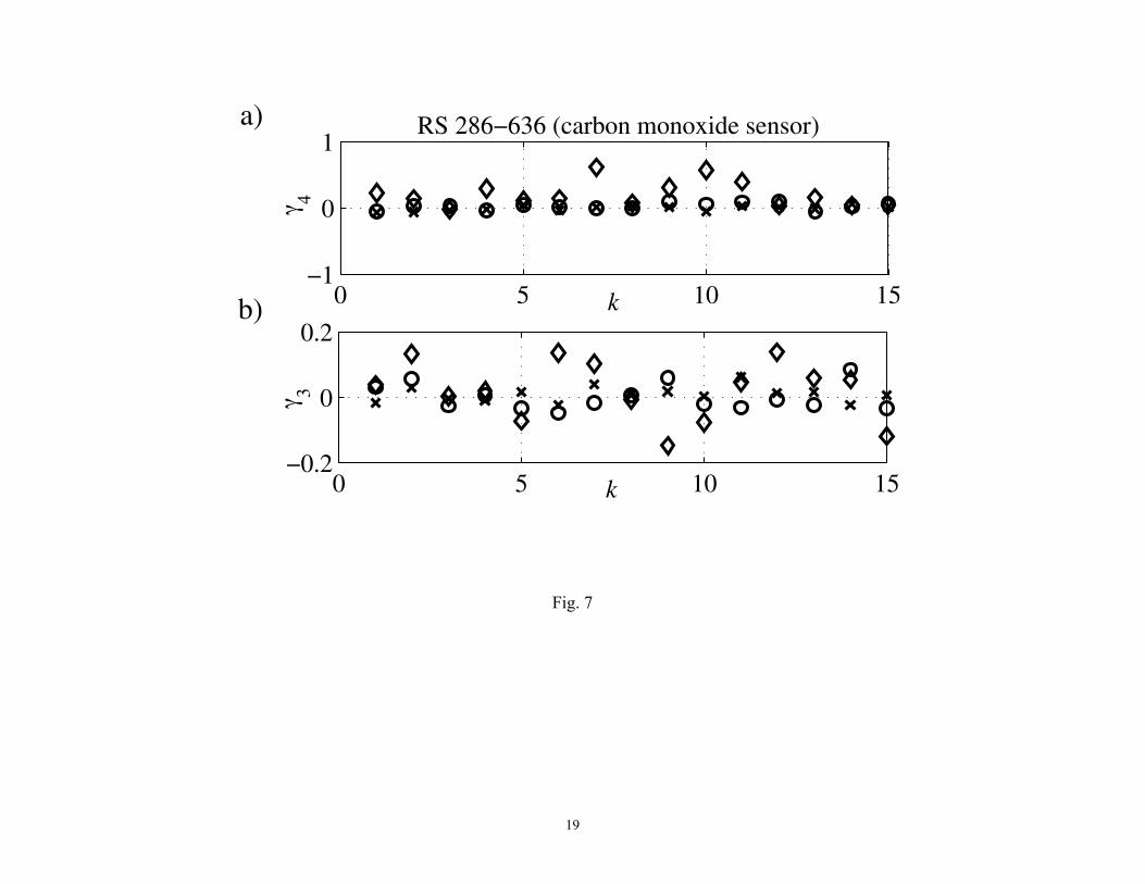
signal. We also ran an alternative test of stationarity. The skewness and the kurtosis were estimated

9
from a very short time record (Fig. 7). No visible trend can be observed, which is in good agreement
with the observed symmetries of the bispectra.
Finally, a few words about the accuracy and the reproducibility of data that are among the
most sensitive issues of chemical sensing efforts.
♦ The fluctuations of the bispectra data were reduced by averaging a large number of records.
This is a more difficult task than doing it with classical power density spectrum. We made
an effort to reduce the fluctuations in the averaged data to a few %. This effort needed quite
much computation time, which was in the order of half hour with present PC computers. As
a result, the bispectrum patterns were fluctuating weakly thus the topology and the basic
shape observed by the naked eye remained the same and only the final details of the curves
showed some fluctuations.
♦ Possible effects of the fluctuations of the ambient gas composition. We controlled the vapor
concentration by control valves (flow meters). The accuracy of the concentration was
supposedly a few %, which is huge compared to the measured stochastic signal. However,
the concentration fluctuations in the ambient gas have a much slower time constant due to
the volume of the sensor chamber, typically in the order of a minute. Taking spectral
considerations into the account, the effects of these slow concentration fluctuations are
reduced at our frequency regime by a factor of 106 - 1010, because the steepness of the cut-
off is at least 20 dB/decade (1/f2 cutoff in the spectrum). We experimentally tested this
hypothesis by switching off the gas flow for a short time. We have not observed any change

10
in the power density spectrum of the measured fluctuations while we were doing that.
4. CONCLUSIONS
Higher-order statistical methods were applied to test the stationarity of the stochastic
component of the signals of Taguchi sensors and to extract additional chemical information from the
non-Gaussian component. Various gas compositions were used. The analysis of kurtosis, skewness
and bispectra indicated that the stochastic signal component was stationary. The bispectra turned
out to be a rich source of additional sensing information which cannot be achieved by measuring the
power spectra or analyzing the resistance in the classical way.
ACKNOWLEDGMENTS
J.S.'s stay at Texas A&M University was sponsored by a NATO Postdoctoral Fellowship and the
Faculty of Electronics, Gdansk University of Technology, Poland. The research was supported by
the Army Research Lab and the Office of Naval Research. A preliminary version of the results was
presented at the SPIE Conference "Noise and Information in Nanoelectronics, Sensors and
Standards", Santa Fe 2003.

11
REFERENCES
1 L.B. Kish, R. Vajtai and C.G. Granqvist: Sensors and Actuators B 71 (2000) 55.
2 A. Hoel, J. Ederth, J. Kopniczky, P. Heszler, L.B. Kish, E. Olsson and C.G. Granqvist: Smart
Mater. Struct. 11 (2002) 640–644.
3 G. Schmera and L.B. Kish: Sensors and Actuators B 93 (2003) 159.
4 J.L. Solis, L.B. Kish, R. Vajtai, C.G. Granqvist, J. Olsson, J. Schnurer and V. Lantto: Sensors
and Actuators B 77 (2001) 312.
5 J. Smulko, L.B. Kish and C.G. Granqvist: Fluctuations and Noise Letters 1 (2001) L147.
6 V. Lantto, P. Romppainen, and S. Leppävouri: Sensors and Actuators B 14 (1988) 149.
7 R.F. Voss: Phys. Rev. Lett. 40 (1978) 913.
8 A.V. Yakimov and F.N. Hooge: Physica B 291 (2000) 97.
9 R. Crook and B.K. Jones: Microelectronics and Reliability 37 (1997) 1635.
10 T. Schreiber and A. Schmitz: Physical Rev. E 55 (1997) 5443.
11 A. Swami and J.M. Mendel: Higher-order spectral analysis toolbox for use with Matlab (The
MATHWORKS Inc., Natick, 1998).
12
FIGURE CAPTION
Fig. 1. The potential barrier between grains in (a) air and (b) reducing gases.
Fig. 2. Symmetry axes of bispectrum function.
Fig. 3. The measurement setup.
Fig. 4. Normalized power spectra of the stochastic signals sampled at frequency fs=20 kHz with
various ambient gas mixtures: a) CO sensor, b) NOx sensor. Synthetic air (solid line), ethanol
70 ppm (dotted line), hydrogen 380 ppm (dashed line).
Fig. 5. Normalized amplitude distribution p(x)/p(0) of voltage noise sampled at frequency
fs = 20 kHz during exposure to synthetic air (solid line), ethanol 70 ppm (dotted line), hydrogen
380 ppm (dashed line): a) CO sensor, b) NOx sensor.
Fig. 6. Bispectra from the CO sensor at a sampling frequency fs = 100 Hz.
Fig. 7. Short-time-estimates of skewness and kurtosis at a sampling frequency fs = 100 Hz with the
CO sensor. Synthetic air (x), ethanol 70 ppm (circle) and alcohol vapor (diamond).

Fig. 1
14
Fig. 2
15
Fig. 3

16
101
102
103
104
10−14
10−12
10−10
10−8
f⋅Sx(f
)/U
2 DC
f [Hz]
RS 286−636 (carbon monoxide sensor)
101
102
103
104
10−12
10−11
10−10
f⋅Sx(f
)/U
2 DC
f [Hz]
RS 286−648 (nitrogen oxide sensor)a) b)
A
A A
A
A
A
A
A
Fig. 4

17
−2 −1 0 1 2
0.2
0.3
0.4
0.50.60.70.8
1RS 286−636 (carbon monoxide sensor)
p(x
)/p(
0)
sign(x)⋅x2/2⋅σ2x
−2 −1 0 1 2
0.2
0.3
0.40.50.60.70.8
RS 286−648 (nitrogen oxide sensor)
p(x
)/p(
0)
a) b)
sign(x)⋅x2/2⋅σ2x
1
Fig. 5
18
Fig. 6
19
0 5 10 15−1
0
1RS 286−636 (carbon monoxide sensor)
γ 4k
0 5 10 15−0.2
0
0.2
γ 3
k
a)
b)
Fig. 7
Recommended
![PRISM: Platform for Remote Sensing using Smartphones · PRISM: Platform for Remote Sensing using Smartphones ... side, however ... sensing enhanced social networking [30],](https://img.pdfslide.us/doc/110x75/5ad4fdb27f8b9a177c8c65f0/prism-platform-for-remote-sensing-using-smartphones-platform-for-remote-sensing.jpg)