High Speed Transport Protocol Test Suite
Romaric Guillier and Pascale Vicat-Blanc PrimetEmail: [email protected]
RESO Team, LIP laboratory

RESO : Protocols and Services for high speed networks,application to Grid Computing
Exploring the limits of the TCP/IP stack in very high
speed networks in a specific application context where:
I The statistical multiplexing is very low
I Protocol (ie TCP) require processing power at the
limit of CPU capacities,
I Data volumes to be transfered are huge
(terabytes),
I Applications are highly delay sensitive (MPI),
I (Co-)allocation of endpoint resources poses
(transfer time constraints).
RESO team contributions concerns:
I Optimisation of communication libraries and
protocol stack implementations for high
performance context (MPI, MX, protocol
offloading)
I Bulk data transfers scheduling problem
formulation and exploration, flow scheduling and
advance (lambda) path reservation services design
(BDTS, SRV)
I High Speed TCP variants evaluation and test suite
development (HSTTS)
I High speed networks monitoring and grid traffic
analysis and modelling (MetroFlux)
I Joint Network and Operating System virtualisation
for Virtual Private Overlay Network management
and optimisation (HIPerCAL)
RESO team collaborates with:
I Grid Community (Grid5000 and Aladdin) - INRIA
NUM-B EPIs
I OGF : Open Grid Forum, IETF (HIP protocol)
and IRTF (TMRG, ICCRG)
I AIST (Japan) , Alcatel-Lucent, France-Telecom
and Myricom
I System@tic, Euro-NGI, ANR & EU FP6-FP7
programs context

Problematic and methodology
ProblematicLegacy Reno TCP is known to be deficient in the
case of high speed networks (congestion avoidance
phase don’t scale). Focus is on the performanceevaluation of new TCP variants (BIC, CUBIC,
HighSpeed-TCP, Hamilton-TCP, Scalable) in highspeed networks with low aggregation level and
symmetric links (ex: Grid networks, FTTH) when
transfering large files.
Ca
C
Aggregation level: K = CCa' 1
Congestion level:∑
Ca
C
Transfer time predictability
I Impact of congestion level?
I Impact of reverse traffic level?
Metrics
I Mean completion time : T = 1Nf
∑Nfi=1 Ti
I Max completion time : Tmax = max(Ti)
I Min completion time : Tmin = min(Ti)
I Std deviation of completion time :
σ =√
1Nf
∑Nfn=1(Ti − T )2
PCSwitch Switch
10Gbps
1Gbps1GbpsPC
Topology
I Classical dumbbell: Nf and Nr pairs of 1 Gbps
nodes
I Network cloud: Grid’5000 backbone, 10 or 1 Gbps
link
I Latency: 19.8 ms or 12.8 ms
I Bottleneck: output port of the L2 switch
Grid’5000
I 9 sites in France, 17 laboratories involved
I 5000 CPUs (currently 3150)
I Private 10Gbps Ethernet over DWDM network
I Experimental testbed for Networking to
Application layers.

Influence of congestion level
Cong.
lvl:∑
CaC
0.9:
280 s/272 s
1.5:
395 s/398 s
2.1:
545 s/535 s
Cubic Scalable
When there is no congestion, flows manage to fully utilise their links.Scalable is displaying a huge variability when there is congestion.There is an asymptotical behaviour of TCP variants when the congestion levelincreases
[TCP variants and transfer time predictability in very high speed networks, Infocom 2007 High Speed Networks Workshop, May 2007]
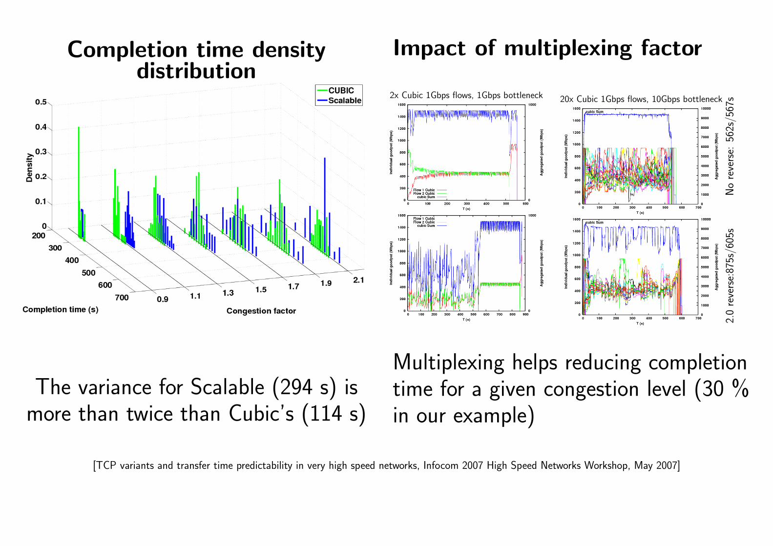
Completion time densitydistribution
The variance for Scalable (294 s) ismore than twice than Cubic’s (114 s)
Impact of multiplexing factor
2x Cubic 1Gbps flows, 1Gbps bottleneck 20x Cubic 1Gbps flows, 10Gbps bottleneck
2.0
reve
rse:
875s
/605
sN
ore
vers
e:56
2s/5
67s
Multiplexing helps reducing completiontime for a given congestion level (30 %in our example)
[TCP variants and transfer time predictability in very high speed networks, Infocom 2007 High Speed Networks Workshop, May 2007]

Influence of reverse traffic on CUBIC (1.5 cong. lvl)
No reverse (395 s) 0.9 reverse (400 s)
1.1 reverse (432 s) 1.5 reverse (438 s)
Reverse traffic has a linear impact on the mean completion timewhen it is congesting the reverse path.The impact is about 1 % when there is no congestion.
[TCP variants and transfer time predictability in very high speed networks, Infocom 2007 High Speed Networks Workshop, May 2007]

High Speed Transport Protocol Test Suite
Two main parts
NXE (Network eXperiment Engine): a generic and
modular Python application to execute
networking scenarios over a given
infrastructure
HSTTS (High Speed Transport Protocol Test Suite):
a set of scenarios representative of real high
speed networks applications.
NXE Workflow description
Topology description
A simple abstract topology description, providing an
easy way to describe the resources and how to exploit
them. Reservation and deployment tools can be easily
switched according to the local nodes management
policy by providing the adequate scripts.
<topology>
<site>
<sitename>sagittaire</sitename>
<number>10</number>
<delay>1</delay>
<nodecapacity>1000</nodecapacity>
<aggreg>AG</aggreg>
<frontal>
<frontalname>lyon.grid5000.fr</frontalname>
<resatool>resa_g5k.sh</resatool>
<resaparam>-w 1:05:00</resaparam>
<deploytool>deploy_g5k.sh</deploytool>
<deployparam></deployparam>
</frontal>
</site>
[..]
<aggregator>
<aggregid>AG</aggregid>
<link>
<from>capricorne</from>
<capacity>10000</capacity>
</link>
<link>
<from>sagittaire</from>
<capacity>10000</capacity>
</link>
</aggregator>
</topology>
Scenario Description
Each node (or set of nodes) involved in the scenario is
given a role (server, client, etc) and a list of execution
steps that will be run during the experiment according
to a centralised relative timer. Separate threads are
used to launch the commands on each node to allow a
greater scalability of the system.
<scenario>
<node>
<id>sagittaire{1-10}</id>
<type>server</type>
<step>
<label>Reno</label>
<date>0</date>
<script>launch_server.sh</script>
<scriptparam>--protocol reno</scriptparam>
</step>
[..]
</node>
<node>
<id>capricorne{1-10}</id>
<target>sagittaire{1-10}</target>
<type>client</type>
<step>
<label>Reno</label>
<date>5</date>
<offset>1</offset>
<script>launch_client.sh</script>
<scriptparam>--protocol reno</scriptparam>
</step>
[..]
</node>
</scenario>

Representative applications
HSTTS provides scenario representative of real
applications used in the context of high speed networks.
TU : Tuning application: a full speed, simple
basic unicast and unidirectional transfer for
benchmarking the whole communication
chain from one source to one sink.
WM : Web surfing applications: a mix of big and
small bidirectional transfers with some delay
constrains (interactive communication)
PP : Peer to peer applications: big bidirectional
transfers.
BU : Bulk data transfer applications:
unidirectional and big transfers like in data
centres or grid context.
PA : Distributed parallel applications:
interprocess communication messages (MPI),
typically bidirectional and small messages
transfers
Each of these applications are defined by the traffic
profile or workload they generate. For instance, the BU
application can be characterised as follows:
I The traffic profile is highly uniform. File sizes are
not exponentially distributed. For example, in
Data Grid like LCG (for LHC) file size and data
distribution are defined by the sampling rate of
data acquisition.
I Packet sizes are mostly constant, with a large
proportion of packets having the maximum size
(1,5KB).
I The ratio between forward-path and reverse-path
traffic depends on the location of the storage
elements within the global grid.
System parameters
These parameters are defined by the infrastructure that
is used to run the experiments.
I RTT
I K = CCa
, the aggregation level (ratio between the
bottleneck capacity C and the access links
nominal capacity Ca)
I Buffer size of the bottleneck
I MTU
I Loss rate
Workload parameters
I Multiplexing factor: M , number of contributing
sources
I Parallel streams: Ns , number of streams used on
each source
I Congestion level: Cg = M∗CaC , ratio between Nf
nodes’ nominal capacity and the bottleneck
capacity
I Reverse traffic level: R , ratio between Nr nodes’
nominal capacity and the bottleneck capacity
I Background traffic: B , type of background traffic
(CBR, VBR) and shape (Poisson, Pareto, Weibull)
Parameter range
Parameter Possible values
InfrastructureRTT (ms) 1 20 200 MixCa (Mbps) 100 1000 10000
K = CCa
1 10 1000
Useful WorkloadM 1 ≈ K � K
Cg = M∗Ca
C 0.8 1.0 2.0Ns 1 5 10
Adv. workloadR 0 0.8 1.5B 0 WMI WMII
HSTTS output example
The following diagram shows the result of a run of the
BU application, with Cg = 1.0 and R = 1.0 between
the Toulouse and Rennes clusters (19.8 ms RTT). The
results are normalised by the performance of Reno
TCP.
The following diagram shows the result of a run of the
PA application, with Cg = 1.0 between the Toulouse
and Rennes clusters (19.8 ms RTT). The results are
normalised by the performance of Reno TCP.
Recommended