8/17/2019 High-speed and high-precision tracking control ofultrahigh-acceleration moving-permanent-magnetlinear synchron…
http://slidepdf.com/reader/full/high-speed-and-high-precision-tracking-control-ofultrahigh-acceleration-moving-permanent-magn… 1/9
Precision Engineering 40 (2015) 151–159
Contents lists available at ScienceDirect
Precision Engineering
journal homepage: www.elsevier .com/ locate /precis ion
High-speed and high-precision tracking control of
ultrahigh-acceleration moving-permanent-magnet
linear synchronous motor
Tadashi Hama, Kaiji Sato∗
Interdisciplinary Graduate School of Science and Engineering, Tokyo Institute of Technology, 4259Nagatsuta, Midori-ku, Yokohama 226-8502, Japan
a r t i c l e i n f o
Article history:
Received 30 May 2014
Received in revised form 7 October 2014
Accepted 30 October 2014
Available online 4 December 2014
Keywords:
Linear motor
Precision
Positioning
Control
Learning
High acceleration
High velocity
a b s t r a c t
This paper describes the high-speed and high-precision tracking control of an ultrahigh-acceleration,
high-velocity linear synchronous motor (LSM). The linear motor can produce a thrust force of more than
3000 N, an acceleration greater than70 G (=686 m/s2), and move at a velocity of over 10 m/s. However, it
has highly nonlinear characteristics, and it is difficult to provide an exact dynamic model for the controller
design. Thus, a suitable controller that does not require a dynamic model in the design was selected and
used for the high-precision tracking control of the linear motor. The design procedure for the suitable
controller consists of two steps. In the first step, a two-degree-of-freedom controller with additional
control elements was designed, and its performance was examined. The additional elements were used to
suppress thenegative influences characterizingpermanent-magnetLSMs with cored electromagnets. The
controller showed high tracking accuracy at low speed, but not at high speed. To overcome this problem,
the controller was improved with a learning control element in the second step. The learning control
element does not require a dynamic model in the design, and it is effective at reducing reproducible errors
at high speed. The effectiveness of the controller was examined and demonstrated experimentally. The
improved controller with the learning control element reduced the maximum tracking error to 1.62m
in the sinusoidal reference motion at a frequency of 20Hz and an amplitude of 10mm.
© 2014 Elsevier Inc. All rights reserved.
1. Introduction
Linear motors are widely used in industrial applications such as
precisionmachine tools, photolithography machines,and assembly
equipment. Linearmotors have fewvibration factors andan advan-
tage in their response because they are directly driven without
power transmissions. Such characteristics are suitable for high-
speed machines [1,2] and precision motion mechanisms [3–8], and
the use of linear motors has increased in recent years [9]. Many
conventional high-speed machines have power transmissions, and
their acceleration and velocity are usually limited to less than 2 G
(=19.6 m/s2) and 2m/s, respectively. However, linear motors are
generallyused when higher acceleration or velocity are demanded.
The required acceleration and velocity have increased yearly,
and many high-speed linear motors have been developed. A lin-
ear motor called a tunnel actuator, which has peculiar-shape cored
electromagnets, achieves an acceleration of 38G [10]. The tubular
∗ Corresponding author. Tel.: +81 45 924 5045; fax: +81 45 924 5483.
E-mail address: [email protected] (K. Sato).
actuator developed for pick and place can move at an acceleration
of 20 G and a velocity of 1.5 m /s [11]. A large-thrust linear motor
that can move at an acceleration of over 27G and at a velocity of
4m/s is commercially available [12].
Permanent-magnet linear synchronous motors (PM LSMs) have
advantages of high controllability and high responsiveness. How-
ever, linear motion mechanisms with PM LSMs also have negative
characteristics that decrease their motion accuracy, for example,
thrust ripple, cogging forces, and friction force. To suppress the
negative characteristics, some controllers have been implemented
with PM LSMs, and their tracking performance has been discussed.
A controller with state feedback elements and a feedforward ripple
compensator provideda tracking performance witha tracking error
within 10m at a maximum velocity and acceleration of 0.5 m/s
and 20m/s2, respectively [13]. The responses of the control system
were examined with desired compensation adaptive robust control
[14]. The tracking error was within 5m at a velocityof 2m/s.
The author’s research group has studied ultrahigh-acceleration
and high-velocity linear motors [15] and have fabricated a moving-
permanent-magnet LSM (MPM LSM) having a thrust-to-mover
mass ratioof 908N/kgwithlow thrustrippleand lowcogging forces
http://dx.doi.org/10.1016/j.precisioneng.2014.11.005
0141-6359/© 2014 Elsevier Inc. All rights reserved.

8/17/2019 High-speed and high-precision tracking control ofultrahigh-acceleration moving-permanent-magnetlinear synchron…
http://slidepdf.com/reader/full/high-speed-and-high-precision-tracking-control-ofultrahigh-acceleration-moving-permanent-magn… 2/9
152 T. Hama, K. Sato / PrecisionEngineering 40 (2015) 151–159
Fig. 1. Experimental setup includingthe prototype MPM LSM. (a) Overall view of theMPM LSM, and (b)measuring system.
[16]. In this study, high-speed and precision tracking control with
an MPM LSM is discussed. As described later, the MPM LSM in this
study is different from the other MPM LSMs introduced in [15,16].
It hasbeen adjusted forease of assembly,and themaximum thrust-to-movermass ratio is smaller than theotherMPM LSMs.However,
the MPM LSM used has a much larger thrust-to-mover mass ratio
than the other linear motors previously reported, and it has the
potential to achieve both high-speed and high-precision motion
with a suitable controller.
This paper describes the high-speed and high-precision track-
ing control of an ultrahigh-acceleration, high-velocity linear motor.
The linear motor has highly nonlinear characteristics, and it is dif-
ficult to use an exact dynamic model in the controller design. Thus,
a controller that does not require a dynamic model in its design
is selected and used for high-precision tracking control of the lin-
ear motor. The design procedure for a suitable controller consists
of two steps. In the first step, a two-degree-of-freedom controller
with additional control elements is designed, and its performance
is examined. The additional elements are used for the suppression
of the negative influences characterizing the PM LSMs with cored
electromagnets.The controllershows high tracking accuracy at low
speed,but notat high speed.For overcoming this problem, thecon-
troller is improved with a learning element in the second step. The
effectiveness of the control system is examined experimentally.
The remainder of this paper is organized as follows. Section 2
explains the structure and the driving principle of the MPM LSM.
In Section 3, the basic causes of the MPM LSM trajectory errors are
described. Then, the controller design based on the simple model
and its control results are described. In Section 4, the controller for
high-speed motion using learning control is explained. Section 5
demonstrates the tracking control results with the learning control
element. Finally, concluding remarks are presented in Section 6.
2. Prototypeof the MPM LSM
Fig. 1 shows a prototype MPM LSM that has been designed to
have an ultrahigh thrust-to-mover mass ratio for ultrahigh accel-
eration and high velocity. The stator of the prototype MPM LSM
consists of two pairs of electromagnet (EM) lines, and its mover is
located between the EM lines. The structures of the stator and the
mover were designed so that the MPM LSM has a high thrust-to-
movermass ratioand a smallthrust ripple. Thebasic structureis the
same asthatof the MPM LSMdescribed in [15,16]. However, theair
gapis widened foreasyadjustment, anddifferentpartsof themover
are used for weight savings. Thelength ofthe EMlineis 2.03m, and
the working range is longer than 1 m. The mover is supported by a
Fig. 2. Structureof themover.
Phase A Phase B
Phase C Phase D
24 48 72 96
18 42 66 90
r r e n t A
12 36 60 84 C u r
6 30 54 78
Position mmFig. 3. Current command signal waveforms.
linearballguideconsisting of four carriagesand twoguiderails. The
displacement of the mover is measured using a laser interferom-
eter with a resolution of 79.1nm (ZLM series, JENAer Metechnik
GmbH).
Each of the EM lines has many core teeth with 100-turn coils,
and the core teeth are arranged at an 18mm pitch. The coils of the
EM are divided into eight phase coils (phase A, B, C, D, and their
reverse phases). Each phase coil is driven by different PWM ampli-
fiers (maximum supply voltage: 280V, maximum supply current:
20A).

8/17/2019 High-speed and high-precision tracking control ofultrahigh-acceleration moving-permanent-magnetlinear synchron…
http://slidepdf.com/reader/full/high-speed-and-high-precision-tracking-control-ofultrahigh-acceleration-moving-permanent-magn… 3/9
T. Hama, K. Sato / PrecisionEngineering 40 (2015) 151–159 153
4000
3000 N
2000
u s t f o r c e N
1000 T h r u
0 5 10 15 200
Current amplitude A
Fig. 4. Measured static thrust characteristic.
Fig. 2 shows the structure of the mover. In the mover, 18 PMs
(NEOMAX-48BH) are arranged at a 24mm pitch. Spacers made of
engineering plastic are inserted between them. The mover is fabri-
cated using light-weight materials such as carbon-fiber-reinforced
plastic (CFRP) and extra super duralumin. The length of the mover
is 440 mm, and the total weight including the carriages and the
sensor target is 4.68kg.
Fig. 3 shows the waveform of the current command signal
applied to the amplifiers for driving the mover. Rectangular sig-nals are used as command signals to generate a large thrust force.
The sign of the current is switched by using the measured position.
Fig. 4 shows the measured static thrust characteristic of the
MPM LSM. Thethrust gain decreaseswith an increase in theapplied
current because of the magnetic nonlinearity.
3. Basic controller design for PM LSMs with cored EMs and
its control performance
3.1. Basic controller structure for the MPM LSM
Two-degree-of-freedom (two-DOF) controllers including a
feedback compensator and a feedforward element are widely used
forhigh response andhigh motion accuracy [17,18]. They are effec-tive for the tracking control of linear motors. Linear motors have
peculiar factors that deteriorate the motion accuracy, and suitable
compensators are needed to decrease the negative influences of
these factors. The MPM LSMs have cored electromagnets in which
the cogging force causes tracking errors. The friction caused in the
linear ball guides also increases the tracking error. Two-DOF con-
trollers with feedforward (FF) elements for cogging and friction
compensation are often used for overcoming these problems in PM
LSMs with cored electromagnets [19,20]. Thus, as a first controller
forthe tracking control of theMPM LSM, a two-DOF controller with
two compensators is designed, and its usefulness is examined.
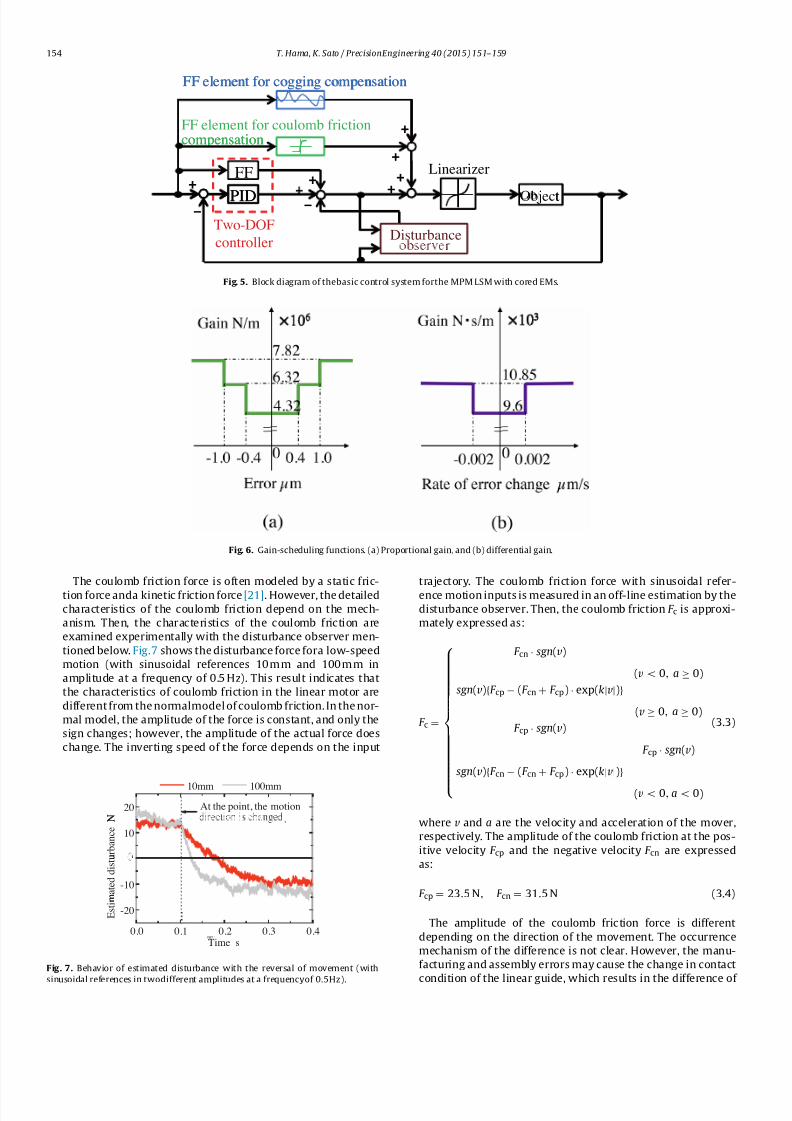
Fig. 5 shows a block diagram of the adopted control system. The
controllerincludes a conventional two-DOF controller for compen-
sating the basic dynamic characteristics of the MPM LSM and theFF elements for compensating the cogging and friction forces. The
conventional two-DOF controller consists of a PID compensator as
a serial compensator and an FF element based on a simple inverse
model of the mechanism. The MPM LSM has high nonlinearity in
the thrust characteristic, and the linearizer for statically canceling
itsnegativeinfluence is inserted between thePID compensator and
the control object. Moreover, a disturbance observer is integrated
in order to compensate for the negative effects caused by model
errors and unknown disturbance forces.
In the control design, a dynamic model is necessary for the dis-
turbance observer andthe FF element in theconventionaltwo-DOF
controller. A detailed dynamic model is generally effective for the
improvement of the tracking performance. However, the MPM LSM
has many nonlinear factors, and it is difficult to model the MPM
LSM accurately. Particularly, it is unrealistic to construct a model
forthe control systemdesign. Thus, a simpledynamic model repre-
sented as a linear mass-damper system is used. The elements and
compensator of the controllers are explained individually.
(a) Nonlinear PID compensator
A nonlinearPIDcompensatoris adopted asa tractableand eas-
ily adjustable series compensator. The compensator includes a
conditional integrator, which operates under the rule described
in Eq. (3.1).
ui =
0,
|uo + ui| > us
and
e · ui ≥ 0
e, otherwise
(3.1)
Here, ui is the integrated value, ui is a variation of the inte-
grated value, e is the error, uo is the sum of the proportional
value and the derivative value, andus is the maximum value of
the control input.
The proportional and derivative elements are gain scheduled
sothatthe movervibration is reduced effectively.Theirgains are
expressedas functionsof an error signaland a time derivative of
an error signal, respectively. The gain functions used are shownin Fig. 6. These were experimentally decided by trial and error
on low speed motions.
(b) FF element for dynamic characteristic compensation
The FF element in the conventional two-DOF controller is
designed based on the simple linear inverse model of the MPM
LSM for dynamic characteristic compensation. Eq. (3.2) repre-
sents the function based on the inverse model,
P inv = m ·( z − 1)2
(T · z )2 + c ·
z − 1
T · z (3.2)
where m is the mass of the mover (m= 4.68 kg), c is the
viscous coefficient (c =30N s/m), and T is the sampling time
(T = 1/16,000s). Eq. (3.2) is derived from the discretization using
the backward differential rule. The rule sometimes makes thesystem sensitive to high frequency noises. However, the elec-
tromagnets of this linear motor have large inductance and work
as noise filter whose cut-off frequencyis lower than 8.5Hz. They
make the system insensitive to high frequency noises.
(c) Linearizer for compensation of nonlinear static thrust charac-
teristic
The MPM LSM used in this study produces a large thrust
force with strong PMs and a large current in the coils. Thus,
the influence of the nonlinearity caused by magnetic saturation
is prominent when a large thrust force is produced. In order to
statically compensate for the nonlinearity of the thrust gain, a
linearizeris implemented. The linearizerwas designed basedon
the measured static thrust characteristic.
(d) FF element for cogging compensationA combination of cored electromagnets and neodymium per-
manent magnets is used for a large thrust force and causes a
large cogging force that deteriorates the tracking performance.
In order to cancel the negative influence of the cogging force,
an FF element is used. The FF element was determined from the
estimatedcogging force as a function of the mover position. The
disturbance observermentionedbelow wasused to estimatethe
cogging force. The cogging force is estimated on the low speed
motion (25mm/s) which does not demand large current. The
large applied current to the linear motor may result in the mag-
netic saturation and influence the cogging force. However, the
influence is ignored in the design of the FF element for cogging
compensation.
(e) FF element for coulomb friction compensation
8/17/2019 High-speed and high-precision tracking control ofultrahigh-acceleration moving-permanent-magnetlinear synchron…
http://slidepdf.com/reader/full/high-speed-and-high-precision-tracking-control-ofultrahigh-acceleration-moving-permanent-magn… 4/9
154 T. Hama, K. Sato / PrecisionEngineering 40 (2015) 151–159
FF element for cogging compensation
FF element for coulomb frictioncompensation
FF element
for
cogging
compensation
+
PID
FF
compensation
Obj t
+ + +
+
+
Linearizer
PID
Disturbance
ect−
−
Two-DOF
controller
Fig. 5. Block diagram of thebasic control system forthe MPM LSM with cored EMs.
Fig. 6. Gain-scheduling functions. (a) Proportional gain, and (b) differential gain.
The coulomb friction force is often modeled by a static fric-
tion force anda kinetic friction force [21]. However, the detailed
characteristics of the coulomb friction depend on the mech-
anism. Then, the characteristics of the coulomb friction are
examined experimentally with the disturbance observer men-
tioned below. Fig.7 shows the disturbance force fora low-speed
motion (with sinusoidal references 10 m m and 100 m m in
amplitude at a frequency of 0.5 Hz). This result indicates that
the characteristics of coulomb friction in the linear motor are
different from the normalmodel of coulomb friction. In the nor-
mal model, the amplitude of the force is constant, and only the
sign changes; however, the amplitude of the actual force does
change. The inverting speed of the force depends on the input
20 At the point, the motion
N
10mm 100mm
10
.
u r b a n c e N
-10
m a t e d d i s t u
0.0 0.1 0.2 0.3 0.4
-20 E s t i m
Time s
Fig. 7. Behavior of estimated disturbance with the reversal of movement (with
sinusoidal references in twodifferent amplitudes at a frequencyof 0.5Hz).
trajectory. The coulomb friction force with sinusoidal refer-
ence motion inputs is measured in an off-line estimation by the
disturbance observer. Then, the coulomb friction F c is approxi-
mately expressed as:
F c =
F cn · sgn(v )
(v < 0, a ≥ 0)
sgn(v ){F cp − (F cn + F cp) · exp(k|v |)}
(v ≥ 0, a ≥ 0)
F cp · sgn(v )
F cp · sgn(v )
sgn(v ){F cn − (F cn + F cp) · exp(k|v |)}
(v < 0, a < 0)
(3.3)
where v and a are the velocity and acceleration of the mover,
respectively. The amplitude of the coulomb friction at the pos-
itive velocity F cp and the negative velocity F cn are expressed
as:
F cp = 23.5 N, F cn = 31.5 N (3.4)
The amplitude of the coulomb friction force is different
depending on the direction of the movement. The occurrence
mechanism of the difference is not clear. However, the manu-
facturing and assembly errors may cause the change in contact
condition of the linear guide, which results in the difference of
8/17/2019 High-speed and high-precision tracking control ofultrahigh-acceleration moving-permanent-magnetlinear synchron…
http://slidepdf.com/reader/full/high-speed-and-high-precision-tracking-control-ofultrahigh-acceleration-moving-permanent-magn… 5/9
T. Hama, K. Sato / PrecisionEngineering 40 (2015) 151–159 155
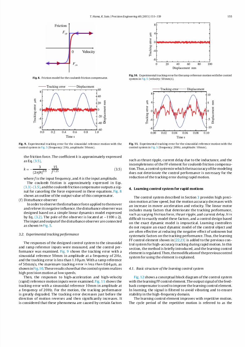
Fig. 8. Friction model for the coulomb friction compensator.
Fig. 9. Experimental tracking error for the sinusoidal reference motion with the
control system in Fig. 5 (f requency: 2 Hz, amplitude: 50mm).
the friction force. The coefficient k is approximately expressed
as Eq. (3.5),
k = −3
(2fA)0.9
−15
f 1.25 (3.5)
where f is the input frequency, and A is the input amplitude.
The coulomb friction is approximately expressed in Eqs.(3.3)–(3.5), andthe coulomb friction compensator outputs a sig-
nal for canceling the force expressed in these equations. Fig. 8
shows an outline of the output value of this compensator.
(f) Disturbance observer
In order to observe thedisturbance force applied to themover
and relieve its negative influence, the disturbance observer was
designed based on a simple linear dynamics model expressed
by Eq. (3.2). The pole of the observer is located at −1100±2 j.
The input and outputof the disturbance observer are connected
as shown in Fig. 5.
3.2. Experimental tracking performance
The responses of the designed control system to the sinusoidaland ramp reference inputs were measured, and the control per-
formance was examined. Fig. 9 shows the tracking error with a
sinusoidal reference 50mm in amplitude at a frequency of 2Hz,
and the tracking error is less than 1.10m. With a ramp reference
of 50mm/s, the maximum tracking error is less than 0.64m, as
shown in Fig.10. These results showthat the control system realizes
high precision motion at low speeds.
Then, the responses to high-acceleration and high-velocity
(rapid) reference motion inputs were examined. Fig. 11 shows the
tracking error with a sinusoidal reference 10mm in amplitude at
a frequency of 20Hz. For the motion, the tracking performance
is greatly degraded. The tracking error decreases just before the
direction of motion reverses and then significantly increases. It
is considered that these phenomena are caused by certain factors
Fig.10. Experimental tracking error for theramp reference motion withthe control
system in Fig.5 (velocity: 50 mm/s).
Fig. 11. Experimental tracking error for the sinusoidal reference motion with the
control system in Fig. 5 (f requency: 20Hz, amplitude: 10mm).
such as thrust ripple, current delay due to the inductance, and the
incompleteness of the FF element for coulomb friction compensa-
tion. Thus, a control systemin which theinaccuracy ofthe modeling
does not deteriorate the control performance is necessary for the
reduction of the tracking error during rapid motion.
4. Learning control system for rapid motions
The control system described in Section 3 provides high preci-
sion motion at low speed, but the motion accuracy decreases with
an increase in mover acceleration and velocity. The linear motor
includes many factors that deteriorate the tracking performance,
such as varying friction force, thrust ripple, and current delay. It is
difficult to exactly model these factors, and a control design based
on the exact dynamic model is impractical. Learning controllers
do not require an exact dynamic model of the control object and
are often effective at reducing the negative effect of unknown but
systematic factors on the tracking performance. Thus, the learning
FF control element shown in [22,23] is added to the previous con-
trol system for high-accuracy tracking during rapid motion. In thissection, the method is briefly introduced, and the learning control
element is regulated. Then, themodificationof thepreviouscontrol
system for using the element is explained.
4.1. Basic structure of the learning control system
Fig. 12 shows a conceptual block diagram of the control system
with the learning FF control element. The output signal of the feed-
back compensator is used to improve the learning control element.
In learning, the signal is filtered to avoid vibrating and to ensure
stability in the high-frequency domain.
The learning control element improves with repetitive motion.
The cycle period of the repetitive motion is referred to as the

8/17/2019 High-speed and high-precision tracking control ofultrahigh-acceleration moving-permanent-magnetlinear synchron…
http://slidepdf.com/reader/full/high-speed-and-high-precision-tracking-control-ofultrahigh-acceleration-moving-permanent-magn… 6/9
156 T. Hama, K. Sato / PrecisionEngineering 40 (2015) 151–159
Feedback
element
+ +
Pl tFeedbackcompensator
− +Plant
Feedforward
Fig. 12. Conceptual block diagram of thelearning control.
0
Fig. 13. Basis functionsof thelearningcontrol.
“movement period.” The basic algorithm for the learning control
is as follows:
u jF
(kh) = u j−1F
(kh) + v j−1(kh) (4.1)
where j denotes the jth repetitive operation, h is the sampling
period, k is the time index, u jF
(kh) is the output of the learning con-
trol element at the time of kh, is the learning gain, and v j−1(kh) is
a value calculated from the next algorithm.
The output of the feedback compensator is filtered by the func-
tion called the “basis function,” and v j(kh) is calculated. Fig. 13
illustrates the basis function used in the learning control. One basis
function has one triangular part in a certain period, and the func-
tion in theother periodequals zero. There arepluralbasisfunctions,
which are named “b1, b2,” according to the emergence order of thetriangular parts in each movement period. Two triangular parts of
the basis functions having adjacent numbers overlap each other.
The output of the feedback compensator is u jc(t ), the function eval-
uation of the basis function bi is defined as i(t ), and the span of
one movement period isN p times the sampling period. Then, v j(kh)
is given by:
v j(kh) =
N i=1
i(kh)
N pl=0
i(lh)u jC
(lh)N pl=0
i(lh)(4.2)
The period of one triangular part in a basis function is 2m times
the sampling period, and the width m determines the width of the
basis function, which influences the bandwidth of the filter.
4.2. Regulation of the learning controller
The learning control element has two significant parameters
that determine its characteristics. One parameter is m, which
decides the width of the basis function. The other is the learning
gain defined in Eq. (4.1). The widthm determines the bandwidth
of the filter. If the width m is small, the control element can also
learn a high-frequency component, but the stability in the high-
frequency domain is reduced. If the width m is large, the stability
of the high-frequency domain is increased, butthe control element
cannot relieve the fast-varying disturbances, and the tracking error
increases with an increase in the input frequency. Fig. 14 shows
the influence of the widthm on the tracking error with a sinusoidal
reference 10mm in amplitude at a frequency of 20Hz. When the
width m is small (m= 15), the amplitude of vibration is larger than
in the case where m is equal to 25. When the width m is large
(m= 40), the fast-varying tracking errors originally caused by the
mechanism are not greatly reduced. The width m was regulated
experimentally, and m=25 was selected as an adequate value. It
is confirmed that the optimum value of the width m is constant
regardless of the frequency of the reference trajectory.
The learning gain determines the speed of learning and influ-
ences the time required for learning and the stability of the control
system. If the gain is large, the time required for learning is
reduced, but the stability of the control system tends to decrease.
The optimum learning gain for the control performance was exam-
ined experimentally, and = 0 .8 was selected regardless of the
reference trajectory.
In order to suppress the negative influence of the current delay
caused by the current amplifiers, the output of the learning control
element is advanced. The optimum time was examined experi-
mentally, and it was decided to advance the output by six times
sampling period.
4.3. Removing the delay element
This control system is required to have a high response perfor-
mance, and a controller including delay elements can deteriorate
the tracking performance. Thus, the integrator is removed. In addi-
tion, the disturbance observer has a delay element and may have
a negative influence on the control performance, although it has a
higherresponseperformance thana simple integrator.Both the dis-
turbance observer and the learning controller have the function of
suppressing effects caused by model errors, butthe combination of
them may also have a negative influence. Then, the influence of the
disturbance observer on the learning control system is examined
experimentally. Fig. 15 shows the response of the learning control
system to a sinusoidal input 10mm in amplitude at a frequency of
20Hz, and the displayed tracking error is measured in the move-
ment period in which the error amplitude is no longer reduced by
the learning control. The gray line represents the tracking error of
Fig. 14. Effect of theparameter m of thelearning control element on thetracking error forthe sinusoidalreference motion (frequency: 20Hz, amplitude: 10mm).

8/17/2019 High-speed and high-precision tracking control ofultrahigh-acceleration moving-permanent-magnetlinear synchron…
http://slidepdf.com/reader/full/high-speed-and-high-precision-tracking-control-ofultrahigh-acceleration-moving-permanent-magn… 7/9
T. Hama, K. Sato / PrecisionEngineering 40 (2015) 151–159 157
Fig. 15. Effect of the disturbance observer on the tracking error of the learning
control system for the sinusoidal reference motion (frequency: 20Hz, amplitude:
10 mm).
the control system with both the learning control element and the
disturbance observer, and the black line represents the tracking
error without the disturbance observer. Both the control systems
can greatly reduce the tracking error and are useful for high-speed
and high-precision tracking control. However, the amplitude of the
tracking error with the disturbance observer is larger than that
of the tracking error without it, and it is shown that the disturb-
ance observer deteriorates the tracking performance in this case.
This study places great importance on the high precision tracking
motion. Thus, it is decided that the disturbance observer is to be
removed although the use of the disturbance observer is expected
to increase the robustness of the control system against sudden
and accidental disturbance force. The learning control system for
therapid motionafterthe modifications mentionedaboveis shown
in Fig. 16.
5. Control results of the learning control system for rapid
motions
The responses of the control system to sinusoidal and ramp
inputs are examined with the learning control system described in
Section 4. In this section, the learning control system is compared
with the control system based on the simple model described in
Section 3 (in this section, it is called “the basic control system”),
and the usability of the controller is discussed. The control results
are shown with regard to the “movement period” (defined in Sec-
tion 4), in which the amplitude of the error is no longer reduced by
the learning control.
5.1. Tracking performance of the sinusoidal referencemotion
Fig. 17 shows the tracking errors with the four different sinu-
soidal references. Table 1 shows thespecifications of theeach inputtrajectory and the maximum tracking errors. The gray and black
lines represent the tracking errors of the basic control system and
the learning control system, respectively.
The learning controller reduces the tracking error in all condi-
tions. In order to discuss the tracking performance, the tracking
errors with two kinds of reference motions are compared. One
motion has a sinusoidal reference 10 mm in amplitude at a
frequency of 20Hz (maximum acceleration: 16.1G, maximum
velocity:1.26m/s);this motion is definedas “motion (a)” in Table 1.
The other motion has a sinusoidal reference 50mm in amplitude
at a frequency of 6 Hz (maximum acceleration: 7.25G, maximum
velocity:1.88m/s); this motionis definedas “motion (d)” in Table 1.
The gray line in Fig. 17(a) shows the tracking error of the former
motion (“motion (a)”), and the gray line in Fig. 17(d) shows the
tracking error of the latter motion (“motion (d)”) with the basic
control system. The maximum error of theformer motion(“motion
(a)”) is 2.9m larger than that of the latter motion (“motion (d)”).
However, with the learning control system, the maximum tracking
error of the latter motion (“motion (d)”) is larger than that of the
formermotion (“motion (a)”) (comparing theblackline in Fig. 17(a)
and the black linein Fig. 17(d)). The maximum acceleration is larger
in the former motion (“motion (a)”), and the maximum veloc-
ity is larger in the latter motion (“motion (d)”). In both motions,
the learning control system reduces the tracking error more effec-
tively than the basic control system. However, in the latter motion
(“motion (d)”), the tracking error becomes large especially around
thepoint of peak velocity,and the performance of thelearningcon-
trol system tends to be affected by the velocity rather than the
acceleration. It is assumed that the change speed of the disturb-
ance force including thrust ripple increases with an increase in the
velocity,and the learning control system cannot reduce thetracking
error effectively. The change in acceleration causes the same effect
as other disturbance forces, but its frequency is as low as that of
the input signal. Thus, the effect of the acceleration is assumed to
be reduced easily by the learning control system, even if the effect
is too large for the basic controller to compensate.
FF element for cogging compensation
FF element for coulomb friction
compensation+
+Learning +
Inverse model of thedynamic characteristic
PD Object+
−
+
+
+
near zercontro er+
Fig. 16. Block diagram of thelearningcontrol systemfor rapid motions.
8/17/2019 High-speed and high-precision tracking control ofultrahigh-acceleration moving-permanent-magnetlinear synchron…
http://slidepdf.com/reader/full/high-speed-and-high-precision-tracking-control-ofultrahigh-acceleration-moving-permanent-magn… 8/9
158 T. Hama, K. Sato / PrecisionEngineering 40 (2015) 151–159
(a) (b)
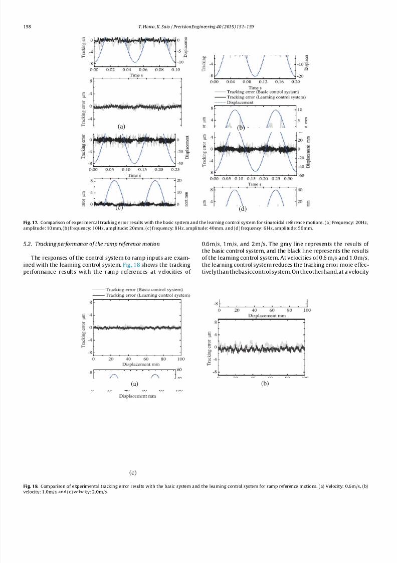
(c) (d)
Fig. 17. Comparison of experimental tracking error results with the basic system and the learning control system for sinusoidal reference motions. (a) Frequency: 20Hz,
amplitude: 10 mm, (b) frequency: 10Hz, amplitude: 20mm, (c) frequency: 8 Hz, amplitude: 40mm, and (d) frequency: 6 Hz, amplitude: 50mm.
5.2. Tracking performance of the ramp reference motion
The responses of the control system to ramp inputs are exam-
ined with the learning control system. Fig. 18 shows the tracking
performance results with the ramp references at velocities of
0.6m/s, 1m/s, and 2m/s. The gray line represents the results of
the basic control system, and the black line represents the results
of the learning control system. At velocities of 0.6 m/s and 1.0m/s,
the learning control system reduces the tracking error more effec-
tivelythan thebasiccontrol system. On theotherhand,at a velocity
(a) (b)
(c)
Fig. 18. Comparison of experimental tracking error results with the basic system and the learning control system for ramp reference motions. (a) Velocity: 0.6m/s, (b)
velocity: 1.0m/s, and (c) velocity: 2.0m/s.

8/17/2019 High-speed and high-precision tracking control ofultrahigh-acceleration moving-permanent-magnetlinear synchron…
http://slidepdf.com/reader/full/high-speed-and-high-precision-tracking-control-ofultrahigh-acceleration-moving-permanent-magn… 9/9
T. Hama, K. Sato / PrecisionEngineering 40 (2015) 151–159 159
Table 1
Specifications of the reference motions and the maximum tracking errors.
Name of motion Reference motion
(frequency and
amplitude)
Maximum
acceleration
Maximum
velocity
Maximum error of
basic control system
Maximum error of
learning control system
(a) 20 Hz, 10 mm 16.1 G 1.26 m/s 5.62m 1.62m
(b) 10 Hz, 20 mm 8.06 G 1.26 m/s 1.86m 1.28m
(c) 8 Hz, 40 mm 10.3 G 2.01 m/s 3.20m 1.68m
(d) 6 Hz, 50 mm 7.25 G 1.88 m/s 2.72m 1.86m
of2.0 m/s, theimprovement in tracking performance is notso effec-
tive in terms of the maximum tracking error.
It is assumed that fast-varying disturbance forces including
thrust ripple mainly deteriorate the tracking performance for the
ramp reference motion. For high-speed motion, the tracking error
with the learning controller is oscillatory due to fast-varying dis-
turbance forces, although it is certain that the learning controller
reduces the amplitude of the tracking error. Meanwhile, for low-
speed motion, the amplitude of the disturbance forces is originally
small. Thus, for a limited velocity range, the learning control sys-
tem shows a large improvement in motion with a ramp reference
compared with the basic control system.
6. Conclusion
In this paper, a controller for high-speed and high-precision
tracking control of an ultrahigh-acceleration and high-velocity
linear motor was designed,and its tracking performance was exam-
ined. First, the tracking control system based on a simple model of
the linear motor was designed. In this control system, the tracking
performance was satisfactory at low speed, and the tracking error
was less than 1.10m with a sinusoidal reference50 mm in ampli-
tude at a frequency of 2Hz. However, the tracking performance
deteriorated for high-acceleration and high-velocity motion. Then,
in order to reduce the tracking error for the motion, a learning
controller that improved the feedforward element in the repetitive
motion was implemented into the control system. This improved
control system greatly reduced the repetitive errors without anaccurate model. For example, the maximum tracking error was
reduced to 1.62m with a sinusoidal reference 10mm in ampli-
tude at a frequencyof 20Hz. The experimentalcontrol results show
that the learning controller can effectively suppress the position-
ing errors that have high-frequency components, and the designed
control system can realize high precision motion performance.
Acknowledgements
The authors would like to thank students T. Imanishi and T.
Taguchi for assisting with the design of the basic control system.
References
[1] KakinoY, MatsubaraA. High speed andhighaccelerationfeeddrivesystem forNC machine tools. IntJ Jpn SocPrecis Eng1996;30(4):295–8.
[2] Suh JD, Lee DG, Kegg R. Composite machine tool structures for high speedmilling machines. CIRP Ann Manuf Technol 2002;51(1):285–8.
[3] Sawano H, Gokan T, Yoshioka H, Shinno H. A newly developed STM-basedcoordinate measuring machine. Precis Eng 2012;36(4):538–45.
[4] FespermanR, Ozturk O, HockenR, Ruben S, Tsao TC,Phipps J, et al. Multi-scalealignment and positioning system – MAPS. Precis Eng 2012;36(4):517–37.
[5] Park CH, Song CK, Hwang J, Kim BS. Development of an ultra prec isionmachine tool for micromachining on large surfaces. Int J Precis Eng Manuf 2009;10(4):85–91.
[6] KimK,ChoiYM,NamBU,LeeMG. Dualservostagewithout mechanicalcouplingfor process of manufacture and inspection of flat panel displays via modulardesign approach. IntJ Precis Eng Manuf 2012;13(3):407–12.
[7] Lee MG, Kim KH, Gweon DG. Novel linear motor for high precision stage of semiconductor lithography system. In: Proc. 17th ASPE annu. meeting. 2002.p. 162–5.
[8] Fukuta M, Nishioka M, Suzuki H. Development of ultra precision machiningwith high positioning resolution. In: Proc. 21st ASPE annu. meeting. 2006.
[9] Oiwa T,Katsuki M, Karita M, Gao W, Makinouchi S, Sato K, et al. Questionnairesurvey on ultra-precision positioning. Int J Autom Technol 2011;5(6):766–72.
[10] Kim HJ, Nakatsugawa J, Sakai K, Shibata H. High-acceleration linear motor,tunnelactuator. J MagSoc Jpn 2005;29(3):199–204.
[11] Messen KJ, Paulides JJH, Lomonova EA. Modeling experimental verification of a tubular actuator for 20-g acceleration in a pick-and-place application. IEEETrans Ind Appl 2010;46(5):1891–8.
[12] Fanuc Corp. FANUC LINEARMOTOR LiS series, catalog; 2012.[13] Braembussche PVD, Swevers J, Brussel HV, Vanherck P. Accurate track-
ing control of linear synchronous motor machine tool axes. Mechatronics1996;6(5):507–21.
[14] Yao B, Hu C, Hong Y, Wang Q. Precision motion control of linear motor drivesystems for micro/nano-positioning. In: Proc. first int. conf. integration andcommercialization of micro and nanosystems. 2007.
[15] Sato K, Katori M, Shimokohbe A. Ultrahigh-acceleration moving-permanent-magnet linear synchronous motor witha longworkingrange.IEEE/ASME TransMechatronics 2013;18(1):307–15.
[16] Sato K. Thrust ripple reduction in ultrahigh-acceleration moving-permanent-
magnet linear synchronous motor. IEEE Trans Magn 2012;48(12):4866–73.[17] Sugiura M, Yamamoto S, Sawaki J, Matsuse K. Thebasic characteristics of two-degree-of-freedom PID position controller using a simple design method forlinear servo motor drives. In: Proc. 4th international workshop on advancedmotion control, vol. 1. 1996. p. 59–64.
[18] Lee C, Salapaka SM. Two degree of freedom control for nanopositioning sys-tems:fundamental limitations, control design, and related trade-offs. In: Proc.American control conference. 2009. p. 1664–9.
[19] Mu HH, Zhou YF, Wen X, Zh ou YH. Calibr ation compens at ion o f cog-ging effect in a permanent magnet linear motor. Mechatronics 2009;19(4):577–85.
[20] Christof R, Andreas J. Motioncontrol of linearpermanent magnet motorswithforce ripple compensation. In:3rd Int. symp lineardrives forindustryapplica-tions (LDIA). 2001.
[21] Olsson H, Astrom KJ, de Wit CC, Gafvert M, Lischinsky P. Friction models andfriction compensation. Eur J Control 1998;4(3):176–95.
[22] Chen YQ, Moore KL, Bahl V. Learning feedforward control using a dilated B-spline network:frequencydomain analysis anddesign.IEEE TransNeuralNetw2004;15(2):355–66.
[23] Chen YQ, Moore KL, Bahl V. Improved path following of USU ODIS by learningfeedforward controller using dilated B-splinenetwork.In: Proc. IEEEint. symp.computational intelligence in robotics and automation (CIRA). 2001. p. 59–64.
Recommended