High Frequency Trading and Market Stability*
Jonathan Brogaard
Thibaut Moyaert
Ryan Riordan
First Draft: October 2013
Current Draft May 2014
This paper investigates the relationship between high frequency traders (HFT) and price
jumps in the stock market. Using the Nasdaq HFT dataset, we find that overall HFT trading
activity is higher around and during price jumps. HFT liquidity taking activity is lower than
normal while HFT liquidity supplying activity is higher. During extreme price jumps HFT
liquidity providers accumulate an inventory position in the opposite direction of the jump.
HFT liquidity takers take an inventory position in the direction of the jump. However, both
positions appear unprofitable. The evidence is generally consistent with HFT dampening
extreme market events.
*The authors are grateful to Nasdaq OMX for providing the data and for the support from the
ARC grant 09/14-025 .
Jonathan Brogaard, University of Washington, e-mail: [email protected]; Thibaut Moyaert, Louvain School of Management, e-mail: [email protected];
Ryan Riordan, University of Ontario Institute of Technology, e-mail: [email protected].

1. Introduction
In the aftermath of the 2008 financial crisis and the May 2010 flash crash the stability
of financial markets has been debated. Market disruptions have numerous implications in
terms of risk management (Duffie and Pan, 2001), derivative pricing (Bates, 2000; Eraker,
Johannes, and Polson, 2003) and portfolio allocation with its influence on the optimal
strategy (Jarrow and Rosenfield, 1984; Liu, Longstaff, and Pan, 2003). While overall market
quality has improved lately (Castura, Litzenberger, and Gorelick, 2010), individual stock
mini-crashes are prevalent (Golub et al., 2013). Those short-lived crashes could originate
from several sources as outlined by Hendershott (2011): HFT activity, market structure
changes, trading fragmentation and/or the disappearance of designed market makers.
In this paper, we analyze the relationship between HFT activity and high frequency
market disruptions. We detect price jumps through the 99.99% percentile of ex-post
observations. We made two cutoffs: idiosyncratic jumps and co-jumps; permanent and
transitory jumps. Co-jumps are jumps that happen simultaneously in several individual
stocks while idiosyncratic jumps are isolated individual stock jumps. A transitory jump is
defined as a jump that reverses within thirty seconds of its inception while a permanent jump
does not reverse in the same time period.
The mechanism of price jumps are not well understood. Farmer, Gillemot, Lillo, Mike,
and Sen (2004) outline that large price fluctuations in a short period of time are driven by
time-varying liquidity supply. On the other hand, Jiang, Lo, and Verdelhan (2010) and Miao,
Ramchander, and Zumwalt (2012) find that most jumps appear at pre-scheduled
macroeconomic news in the US treasury bond market and in the stock index futures market.
High frequency trading (HFT) activities are often accused of triggering or enhancing these
events. In response to these concerns exchanges and regulators have already taken action.
The Euronext stock exchange now imposes a cancelation fee to avoid the implementation of
some HFT strategies. Several regulators are discussing the implementation of minimum
liquidity provision by HFT firms.
Price jumps could be affected by HFT in several ways. In times of heightened market
instability, when price jumps are more likely to occur, HFT firms may exit the market or
could add to one-sided order imbalance, which could ignite or enhance a jump in prices. If so,
the observation that HFT firms provide liquidity on average may hide that in times of market
instability they switch from liquidity provision to liquidity taking.
We use the Nasdaq HFT dataset used in other research (e.g. Brogaard, Hendershott,
and Riordan, 2013). The data divides market participants into two types, HFT and non-HFT
(nHFT). The data also disclose which type of participant is taking and providing liquidity for
each trade.
We find HFT do not cease their trading activity during or around price jumps.
Moreover the increase in HFT activity is on their passive trading activity. Then, we
investigate HFT/nHFT net volume around jumps. HFT and nHFT trade on average
aggressively when in direction of the price jump and passively when against the price jump
direction. In net, we find that neither HFT nor nHFT exhibit a significant net position for
supply-driven jumps (midquote jumps) while demand-driven jumps (transaction jumps)
unveil that HFT holds a significant contrarian net position during jumps.
The likelihood of a permanent price jump to occur is higher when lagged HFT net
volume is in the direction of the price jump. At the opposite, transitory price jumps go along
with HFT net volume against the price jump direction. It reflects that HFT activity can be
related to a quicker adjustment of prices to information which in turn may explain the
prevalence of stock specific price jumps.
The remainder of the paper proceeds as follows. Section 2 provides a review of the
existing literature. Section 3 describes the data set used in this paper. Section 4 presents the
applied methodology. Section 5 reports the empirical results. Section 6 concludes.

2. Literature Review
High frequency trading (henceforth HFT) is one of the latest major development in
financial markets. The investigation of its externalities in the market is of utmost importance
given its prominence. Indeed, several papers (Zhang, 2010; Brogaard, 2011) estimate that
HFT accounts for about 70% of trading volume in the U.S. capital market as from 2009.
A comprehensive definition of what HFT activities include remains elusive. According
to Castura, Litzenberger, and Gorelick (2010), it encompasses professional market
participants that present some characteristics: high-speed algorithmic trading, the use of
exchange co-location services along with individual data feeds, very short investment horizon
and the submission of a large number of orders during the continuous trading session that
are often cancelled shortly after submission.
The existing literature outlines overall that HFT activity improves market quality.
Indeed, the rising of HFT activity went along with a reduction of the spread, a liquidity
improvement and a reduction of intraday volatility (Castura, Litzenberger, and Gorelick,
2010; Angel, Harris, and Spatt, 2010; Hasbrouck, and Sarr, 2011). Hanson (2011) and
Menkveld (2012) even describe HFT as the new market makers in U.S. financial markets.
Indeed, HFT acts mostly as liquidity providers and engages in price reversal strategies
(Brogaard, 2011).
Lately HFT activity was under the spotlight following the liquidity-induced flash crash
on May 6th, 2010 that casts doubt on the soundness of HFT activity and its externalities on
market stability and price efficiency.
Golub, Keane and Poon (2013) document that along with a market quality
improvement, individual stock mini-crashes are prominent as well. Hendershott (2011) puts
forward several potential origins of those liquidity-driven crashes such as high frequency
trading activity, market structure changes, trading fragmentation and/or the disappearance
of designed market makers.

In this paper, we document the relationship between HFT and market stability. We
isolate period of instability by looking at high frequency market disruptions and investigate
the behavior of HFT from a microstructure viewpoint during those periods. Our focus
straddles two literatures. First, we briefly review the literature on the link between price
movements and liquidity provision. Second, we summarize the expanding literature on HFT
and market stability.
Several papers document the relationship between order book imbalances and price
movements. Chordia and Subramanyam (2004) report a positive correlation between daily
order book imbalance, stock returns and volatility. Chordia, Roll, and Subramanyam (2008)
also highlight that return predictability is lower when the spread is tight. Cao, Hansch, and
Wang (2009) investigate the informational content of the order book and show it fosters
price discovery in the market.
On higher frequency aggregation sampling, Harris and Panchapagesan (2005)
confirm a relationship between the limit order book and future price movements. Hellström
and Simonsen (2009) point out that the information content of the order book is short-lived.
Indeed, they find some predictability at a 1 and 2-minute aggregation sampling on the
Stockholm stock exchange while it vanishes quickly on lower frequency sampling.
The relationship between market disruptions and liquidity provision is not
straightforward and depends on the market.
The consensus is that the jump frequency observed in the stock market is not fully
explained by news, whether macroeconomic or firm specific. Indeed, Farmer, Gillemot, Lillo,
Mike, and Sen (2004) show that the trigger of large price fluctuations on the London Stock
Exchange is time-varying liquidity supply. Hence, jump risks is stock specific. Illiquid stocks
tend to suffer from jumps more often than liquid ones. Consistent results are found on US
market data. Joulin, Lefevre, Grunberg, and Bouchaud (2008) and Weber and Rosenov
(2005) document that the root of price jumps is a lower density of the order book in spite of

the surge of significant trading volume underlying the arrival of information. Lately, Boudt,
Ghys, and Petitjean (2012) estimate that around 70% of jumps are liquidity-related on the
DJIA index. They emphasize that the effective spread and the number of trades is informative
of forthcoming jumps.
Recent papers (Jiang, Lo, and Verdelhan, 2010; Miao, Ramchander, and Zumwalt,
2012) on the US treasury bond market and in the stock index futures market contrast those
results. They show that the majority of price jumps appear at pre-scheduled macroeconomic
news.
Market instability is by definition a rarely occurring event which makes it a
challenging issue to investigate. The behavior of HFT during those periods of instability
remains broadly unexplored. The flash crash on May 6, 2010 is often given as an example of
HFT deteriorating market stability. However, it relies on the strong assumption that the
market would behave in a given way in the absence of HFT. Furthermore, the potential
impact of a trader is related to its position. In this view, non-HFT who could attempt to
buy/sell a large position quickly are more of a threat to market stability than HFT who
typically limit their positions in a market.
Brogaard, Hendershott, and Riordan (2013) show that HFT activity is positively
correlated to public information, market-wide movements and limit order book imbalances.
This higher HFT activity doesn't seem to prevent from market overreaction. Indeed,
Kirilenko, Kyle, Samadi, and Tuzun (2011) highlight that while the flash crash was originated
by a bad execution of a large order initiated by a non-HFT trader, HFT exhibits abnormal
behaviors and exacerbates market volatility that day.
Several papers outline a tight relationship between high frequency activity and stock
specific volatility (Brogaard, 2012; Zhang, 2010; Kirilenko, Kyle, Samadi, and Tuzun, 2011).
This higher stock price volatility could be the results of the interaction between HFT traders
and fundamentals traders (Zhang, 2010).

Theoretically, Biais, Foucault, and Moinas (2012) develop a framework where they
show that HFT traders increase adverse selection costs for non-HFT traders. Jovanovic and
Menkveld (2011) found similar results. This additional adverse selection cost comes from the
higher speed of information processing by HFT. Foucault, Hombert, and Rosu (2012) show
that this speed advantage leads to a higher fraction of trading volume that is made by
informed traders, it increases trading volume, decreases liquidity, induces price changes that
are more correlated with fundamental value movements, and reduces informed order flow
autocorrelations.
Bernales (2013) outlines that HFT traders are more profitable in high volatile periods
(volatility shocks), which suggests they may have an incentive to manipulate market
volatility. In a theoretical framework, Goettler, Parlour, and Rajan (2009) found that the
limit order market acts as a "volatility multiplier" in that prices are more volatile than the
fundamental value of the asset. This is all the more true when the fundamental volatility of
the asset is higher or when there is information asymmetry across traders.
In this framework, market stability could be affected by HFT controversial strategies
that could indirectly generate volatility in the market. Hendershott, Jones, and Menkveld
(2011) outline that over 90% of the orders submitted by HFT are either cancelled or modified
(cancelled and resubmitted) before being filled. Lately, Gai, Yao, and Ye (2012) show that
HFT increases the order cancellation/execution ratio, which supports the significant
implementation of quote stuffing1, and layering2 strategies in the market. Finally, Egginton,
Van Ness, and Van Ness (2013) show that quote stuffing is ubiquitous in the US stock market.
They find that stocks that experience quote stuffing display lower liquidity, higher trading
costs, and higher short term volatility. Lately some regulators consider imposing a
cancellation fee to prevent HFT potential detrimental externalities on the stock market. There
is also talks to impose obligations on HFT to provide a minimum amount of liquidity and
1 Quote stuffing consists in submitting a large number of orders followed immediately by a cancellation
to generate order congestion. 2 Layering consists in submitting a large number of orders in one side of the book that are not meant to
be filled to facilitate the entry on the other side of the book.

prevent in such a way monetary drying up of liquidity, a role that was ensured previously by
designed market makers.
On the other hand, market quality improves mainly as from 2006 and is tough to
relate directly to the emergence of HFT activity (Castura, Litzenberger, and Gorelick, 2010).
Indeed, almost at the same time, the market structure acknowledges major changes both in
the U.S. and in Europe with respectively the implementation of RegNMS and MiFID.
Furthermore, Golub et al. (2013) document that individual stock mini-crashes are prominent
along with overall market quality improvement. Hendershott (2011) puts forward several
potential origins of those liquidity-driven crashes; among them high frequency trading
activity.
Some papers report a tight relationship between high frequency activity and stock
specific volatility (Kirilenko, Kyle, Samadi, and Tuzun, 2011; Zhang, 2010; Brogaard, 2012).
Indeed, HFT generates the majority of order flow while it displays periodicity in order
submission and a high rate of order cancellations and modifications. Significant changes in
their market activity from liquidity providers to liquidity takers suggest HFT may emphasize
volatility/price movements and cause overreaction in the market.

3. Data
The database consists in 40 large m arket capitalization stocks that are listed half-
and-half on NASDAQ and the New York Stock Exchange (NYSE).3 It is the same data used in
other academic studies including Brogaard, Hendershott, and Riordan (2013) and O’hara,
Yao, and Ye (2013).
The data spans two years from January 1, 2008 to December 31, 2009. NASDAQ
categorizes market participants as a high-frequency trading firm or non-high-frequency
trading (nHFT) firm, which allows us to identify investor types. A limitation of using market
participant identifiers (MPIDs) is that NASDAQ is unable to disentangle HFT activity by large
integrated firms that also engage in low-frequency trading strategies. Our data covers trading
activity on the NASDAQ trading venue, other trading venues activity is thus not accounted for
in this paper.
The dataset identifies 26 HFT firms that act as independent HFT proprietary trading
firms.4 The dataset includes whether the buyer or seller initiated the trade and identifies the
type of trader on both sides of the trade.
We supplement the NASDAQ HFT dataset with the National Best Bid and Offer
(NBBO) from TAQ. The NBBO measures the best prices prevailing across all markets to focus
on market-wide price discovery.
We remove trades that occur before 9:30 and after 16:00 as well as trades that take
place during the opening and closing auction to focus on the stock market continuous trading
hours. The filtered database consists in 41,342,013 10-second intervals.
3 NASDAQ OMX provides us the HFT database to academics under a non-disclosure agreement. Our
data covers stocks such as Apple and GE. 4 Some HFT firms were consulted by NASDAQ in the decision to make data available. No HFT firm
played any role in which firms were identified as HFT and no firms that NASDAQ considers HFT are excluded. While these 26 firms represent a significant amount of trading activity and according to NASDAQ fit the characteristics of HFT, determining the representativeness of these firms regarding total HFT activity is not possible.

4. Methodology
From the millisecond time-second trades we arrange the database into 10-second
intervals to detect market disruptions.5
We consider the 99.99% percentile of ex-post observations as a threshold for a price
jump. This straightforward methodology assumes static volatility which makes it a
questionable proxy. Nevertheless, it offers a good compromise at very high frequency
sampling scheme as more robust jump tests accuracy tends to be affected by microstructure
noise. We investigate several jump cutoffs in the paper. 6
First, midquote versus transaction jumps. Midquote jumps are extreme midquote
changes during a 10-second interval while transaction jumps are extreme transaction price
changes during the same interval. Both jumps offer insights since it can be seen as a liquidity
supply jump (midquote jump) or a liquidity demande jump (transaction jump). For the sake
of simplicity, we focus on midquote jumps in the core of the text and refer to transaction
jumps when it holds additional insight compared to misquote jumps.
Second, permanent versus transitory jumps. A transitory jump is defined as a jump
that fully reverses within 30 seconds of its inception while a permanent jump does not fully
reverse in the short run.
Finally, we disentangle idiosyncratic versus co-jumps. Co-jumps are jumps that occur
in several stocks within a small period of time. In the core of the paper, we set the definition
to jumps that occur in at least 10% of our sample stocks within the same minute. By contrast,
idiosyncratic jumps are “isolated” individual stock jumps.
5 We repeat the analysis with 1 minute, and 5-minute intervals to control for the robustness of our results. Those results are available upon request. 6 We carry out several robustness checks on our initial cutoffs that are not reported in the paper. Those results are available upon request.
Table 1 reports descriptive statistics of some microstructure variables during and
around jumps.
INSERT TABLE 1 ABOUT HERE
Panel A reports all jumps descriptive statistics while Panel B and C highlights
respectively the permanent and transitory cutoffs. Price dynamics unsurprisingly unveil a
spike during the jump interval. Transitory jumps exhibit a wider scope than permanent
jumps on average. The t+1 return shows the interval following jump inception is a pullback
on average for transitory jumps while permanent jumps acknowledge no pullback. The
trading volume both in shares and in US dollar is higher during the jump interval. Again
transitory jumps go along with more trading activity than permanent jumps both during and
around the jump interval. As expected, the net overall volume (in shares and in US dollar) is
in the price jump direction. Net overall volume reverses after the jump inception for
transitory price disruptions while it only moderates for permanent price jumps. Overall, we
find that transitory price disruptions happen in a lower liquidity market context than
permanent price disruptions. Indeed, the spread is wider and the depth lower for transitory
jumps compared to permanent ones. Liquidity conditions (spread and depth) tend to
improve for both permanent and transitory jumps.
Using the 99.99% percentile methodology and a 10-second window we isolate 3,431
jumps. Most of those jumps are permanent (2,669) with transitory jumps (762) that yields
only for about a fifth of all price jumps. By definition the percentile definition is roughly
evenly distributed among stocks, small differences arise from no trading intervals.
Table 2 displays the Pearson correlation coefficients for all the variables of interest in
this paper. Overall we mention a correlation especially between price dynamics, volume in
shares and in US dollar, net volume in shares and in US dollar. Net volume is positive
correlated with HFT and nHFT demand while negatively correlated with HFT and nHFT
supply. It suggests that imbalance in trading activity comes mainly from aggressive trading
for both HFT and nHFT. HFT Net volume demand/supply and nHFT net volume
demand/supply are positively related. At the opposite, net HFT demand is higher when there
is less nHFT net volume supply and vice versa.
INSERT TABLE 2 ABOUT HERE
5. Trading Behavior
a. Summary
We find HFT do not cease their trading activity during or around price jumps. Instead
HFT trading activity significantly increases in such market condition. Looking more into
details, we show that it is passive HFT trading activity that spike while aggressive trading
activity remains broadly unchanged.
To investigate the one-sided of the order book activity, we report HFT/nHFT net
volume around jumps. HFT and nHFT trade on average aggressively when in direction of the
price jump and passively when against the price jump direction. In all, we find that neither
HFT nor HFT exhibit a significant net volume pattern for supply-driven jumps (midquote
jumps) while demand-driven jumps (transaction jumps) unveil that HFT are price reversal
during such market disruptions. The permanent/transitory cutoff supports our initial finding.
The likelihood of a permanent price jump to occur is higher when lagged HFT net
volume is in the direction of the price jump. At the opposite, transitory price jumps go along
with HFT net volume against the price jump direction. It reflects that HFT activity can be
related to a quicker adjustment of prices to information which in turn may explain the
prominence of stock specific price jumps outlined in Golub et al. (2013).
The size of the jump is mostly due to market condition. Volatile market environment
(low depth and wide spread) as well as the sudden surge of trading volume are positively
correlated to the jump size.

To evaluate whether HFT firms may have an incentive to try and trigger market
disruptions, we evaluate their trading profits around price jumps. The results suggest that
HFT firms have no obvious incentives to foster the inception of disruptions. Overall, nHFT
make profit on their aggressive trading activity while HFT lose money on their passive
trading activity during the jump interval. In all, we find no significant profit patterns during
price jumps whether for HFT or nHFT.
b. HFT trading volume around jumps
A first concern that is often mentioned when market acknowledges unstable period is
that HFT may withdraw the market. In this first table we investigate the HFT trading activity
in share in the market and consider three cutoffs: All trading activity, Aggressive trading
activity and passive trading activity.
Table 3 outlines HFT do not cease or even decrease its activity during and around
jumps. Indeed, HFT activity is 18% higher during jump interval compared to non-jump
interval. This higher HFT trading activity is also true 10-second prior and after the jump
interval with an increase HFT activity of 30%. nHFT display similar patterns with a 50+%
increase in trading volume for both passive and aggressive trading activity.
INSERT TABLE 3 ABOUT HERE
Looking at the splitting HFT aggressive/passive trading activity, it shows the spike of
HFT trading activity is mainly due to the increase of HFT passive activity with an abnormal
activity level of more than 30% while HFT aggressive activity is close to its normal market
condition level and even below during the jump interval. It suggests that HFT increase their
liquidity provision in times of market instability.

c. HFT net volume around jumps
Table 4 depicts HFT and nHFT net volume during and around price jumps as well as
for the idiosyncratic/cojumps cutoff. All in all, HFT and nHFT exhibit similar behavior. They
trade aggressively in the direction of the jump and against the direction of the jump, they
trade passively. HFT net all volume is on average in the direction of the jump but not
significant. It is also worthwhile to mention that HFT tend to become significantly aggressive
the interval prior to a jump inception while nHFT are still net liquidity provider. Focusing on
the cojumps/idiosyncratic cutoff, HFT are only more aggressive during the cojump interval
while HFT already start their aggressive activity in the prior interval to jump occurrence.
Table 5 is a robustness check on transaction jumps instead of midquote jumps. It
confirms the trading behaviors of both HFT and nHFT. The overall net volume of HFT and
nHFT yields interesting insights. It supports the idea that HFT exhibit a significant price
reversal behavior during price jumps. The idiosyncratic/cojumps cutoff draws the same
conclusion even though HFT net volume is more pronounced for idiosyncratic jumps than for
cojumps. It is in line with more trading activity and net volume position in the case of
transitory jumps compared to permanent ones.
INSERT TABLES 4 AND 5 ABOUT HERE
All our results suggest neither HFT nor nHFT have a significant net volume position
during the jump interval for midquote jumps. At the opposite, transaction jumps confirm
HFT acts as market makers while nHFT display net volume in the jump direction. It is also
worthwhile to outline that the scope of the imbalance is much more sizeable for nHFT than
for HFT which supports that HFT does not hold a significant inventory during the continuous
trading day.

d. HFT net volume around permanent/transitory jumps
Tables 6 and 7 report HFT and nHFT net volume during and around
permanent/transitory price jumps. It support our initial finding in that HFT and nHFT
exhibit similar behavior on average with aggressive trading in the jump direction and passive
trading in the opposite jump direction. The size of net volume activity is more pronounced in
the case of permanent jumps than transitory ones. Again, we point out to HFT as being
market markers in the case of transaction jumps while midquote jumps unveil no significant
patterns whether from HFT or nHFT.
INSERT TABLES 6 AND 7 ABOUT HERE
e. Drivers of price jumps occurrence
In Table 8, we investigate the drivers of price jumps in the stock market. For this
purpose, we first control for a series of microstructure variables. Price jumps tend to happen
in a low liquidity time period. Indeed, we find that a wide spread and a lower depth increase
the likelihood of price jump occurrence. To the same extend, we outline that higher lagged
trading volume both in shares and in US dollar goes along with more jumps. Price dynamics
also outline a more volatile market environment.
Looking at the permanent/transitory cutoff, we show that lagged HFT net volume in
the jump direction increase the probability of a jump to occur. During permanent price
jumps, nHFT are aggressive against the jump direction while HFT net passive volume is in
the jump direction during and prior the jump occurrence. At the opposite, HFT net volume is
against the jump direction during transitory jumps. Prior to the jump, we outline that HFT
net aggressive volume is significant and in the jump direction while nHFT provide liquidity in
the jump direction.
INSERT TABLE 8 ABOUT HERE

f. Drivers of price jumps size
Table 9 points out to the positive relation between the size of permanent jumps and
lagged volatility measure (High Low and Squared return). A sudden surge of trading volume
(significantly lower prior to jump and significantly higher during the price jump) is another
driver of permanent jump size. The depth at the best quote is also informative for a large
jump size. HFT net trading activity shows that the size of permanent jump is larger when
HFT trade aggressively in the jump direction. At the opposite the size of transitory jumps
seem to be related to dollar trading volume during the jump interval. There are also bigger
when lagged return is small. HFT and nHFT trading behavior seem to have no effect on the
size of transitory jumps.
INSERT TABLE 9 ABOUT HERE
g. Profitability
To more accurately discern HFT firms’ interest and anticipation of price jumps, we
analyze HFT profits during market dislocations.
Table 10 shows HFT and nHFT profit around jumps as well as profit for the cutoff
permanent/transitory. All in all, we find that HFT tend to incur losses on average during
market disruptions while nHFT make profit on average. Nevertheless, few significant
patterns appear in a 10-second interval. Overall nHFT make profit on their aggressive trading
activity during jumps while HFT lose money on their liquidity supply activity. At a 90%
confidence interval, we confirm this finding on all trading activity with HFT losing money at
the expense of nHFT during price jumps.

We cannot associate permanent price jumps with any significant profit patterns for
whether HFT or nHFT. Still on average, we find that HFT exhibit a negative PnL at the
opposite of nHFT.
Finally, HFT profits are statistically insignificantly different from zero for transitory
jumps. The splitting of aggressive and passive trading activity unveils that HFT incur a loss
on their liquidity provision while nHFT make profit on their aggressive trading activity at a
90% confidence interval. This behavior is consistent with HFT firms acting as market
markers.
INSERT TABLE 10 ABOUT HERE
6. Conclusion
In this paper, we take advantage of a NASDAQ HFT dataset that identifies investor
types (HFT and non-HFT) to investigate the relationship between HFT activity and market
disruptions. Market disruptions are detected using a straightforward 99.99% percentile. We
cutoff idiosyncratic jumps (isolated individual stock jumps) and co-jumps (jumps that occur
simultaneously in several individual stocks).
We find HFT are more active during market disruptions. It suggests that HFT process
information quicker than nHFT and act as the main liquidity providers in time of higher
information asymmetry.
We investigate the one-sided order book activity for HFT/nHFT around jumps. On
average, they trade aggressively when in direction of the price jump and passively when
against the price jump direction. In all, we find that neither HFT nor HFT exhibit a
significant net volume pattern for midquote jumps while transaction jumps confirm that HFT
are implementing price reversal strategies during such market disruptions.

The likelihood of a permanent price jump to occur is higher when lagged HFT net
volume is in the direction of the price jump. It reflects that the higher HFT activity leads to a
quicker adjustment of price to information, which in turn may explain the prominence of
stock specific price jumps outlined in Golub et al. (2013). At the opposite, transitory price
jumps go along with HFT net volume against the price jump direction.
The size of the jump is mostly due to market condition. Volatile market environment
(low depth and wide spread) as well as the sudden surge of trading volume are positively
correlated to the jump size.
To evaluate whether HFT firms may have an incentive to try and trigger market
disruptions, we evaluate their trading profits around price jumps. The results suggest that
HFT firms have no obvious incentives to foster the inception of disruptions. Overall, nHFT
make profit on their aggressive trading activity while HFT lose money on their passive
trading activity during the jump interval. In all, we find no significant profit patterns during
price jumps whether for HFT or nHFT.
References
Akaike, H. (1974). A new look at the statistical model identification. Automatic Control IEEE 19(6), 716-723. Andersen, T., T. Bollerslev, P. Frederiksen, and M. Nielsen (2010). Continuous-time models, realized volatilities, and testable distributional implications for daily stock returns. Journal of Applied Econometrics 25, 233-261. Andersen, T., D. Dobrev, and E. Schaumburg (2012). Jump-robust volatility estimation using nearest neighbor truncation. Journal of Econometrics 169, 75-93. Angel, J., L. Harris, and C. Spatt (2010). Equity trading in the 21st century. Working paper. Bajgrowicz, P. and O. Scaillet (2011). Jumps in high-frequency data: spurious detections, dynamics, and news. Swiss Finance Institute, 11-36. Bakshi, G. and G. Panayotov (2010). First-passage probability, jump models, and intra horizon risk. Journal of Financial Economics 1 (95), 20-40. Barndor-Nielsen, O. and N. Shephard (2004). Power and bipower variation with stochastic volatility and jumps. Journal of Financial Econometrics 2 (1), 1-48. Bates, D. (2000). Post'87 crash fears in S&P 500 futures option market. Journal of Econometrics 94, 181-238. Bernales, A. (2013). How fast can you trade? HFT in dynamic limit order markets. Working paper. Biais, B., T. Foucault, and S. Moinas (2012). Equilibrium high frequency trading. Working paper. Boudt, K., C. Croux, and S. Laurent (2011). Robust estimation of intraweek periodicity in volatility and jump detection. Journal of Empirical Finance 18 (2), 353-367. Boudt, K., H. Ghys, and M. Petitjean (2012). Intraday liquidity dynamics of DJIA stocks around price jumps. Working Paper. Brogaard, J. A. (2011). High frequency trading and its impact on market liquidity. Working Paper. Brogaard, J. A. (2012). High frequency trading and volatility. Working Paper. Brogaard, J. A., T. Hendershott, and R. Riordan (2013). High frequency trading and price discovery. Working Paper. Cao, C., O. Hansch, and X. Wang (2009). The information content of an open limit-order book. Journal of Futures Markets 29 (1), 16-41. Castura, J., R. Litzenberger, and R. Gorelick (2010). Market efficiency and microstructure evolution in the U.S. equity markets: A high frequency perspective. Working paper-RGM advisors. Chordia, T., R. Roll, and A. Subrahmanyam (2008). Liquidity and market efficiency. Journal of Financial Economics 87, 249-268.

Chordia, T. and A. Subrahmanyam (2004). Order imbalance and individual stock returns: Theory and evidence. Journal of Financial Economics 72, 485-518. Cont, R., A. Kukanov, and S. Stoikov (2011). The price impact of order book events. Working paper. Duffie, D. and J. Pan (2001). Analytical value-at-risk with jumps and credit risk. Finance and Stochastics (5), 155-180. Dufour, A. and R. Engle (2000). Time and the price impact of a trade. Journal of Finance 55(6), 2467-2498. Egginton, J., B. Van Ness, and R. Van Ness (2013). Quote stuffing. Working paper. Engle, R. and J. Lange (2001). Predicting VNET: A model of the dynamics of market depth. Journal of Financial Markets 4, 113-142. Eraker, B., M. Johannes, and N. Polson (2003). The impact of jumps in volatility and returns. Journal of Finance 58, 1269-1300. Farmer, J. D., L. Gillemot, F. Lillo, S. Mike, and A. Sen (2004). What really causes large price changes? Quantitative Finance 4 (4), 383-397. Foucault, T., J. Hombert, and I. Rosu (2012). News trading and speed. Working paper. Gai, J., C. Yao, and M. Ye (2012). The externalities of high-frequency trading. Working paper. Goettler, R., C. Parlour, and U. Rajan (2009). Informed traders and limit order markets. Journal of Financial Economics 93 (1), 67-87. Golub, A., J. Keane and S-H. Poon (2013). High Frequency Trading and Mini Flash Crashes. Working paper Hanson, T. A. (2011). The effects of high frequency traders in a simulated market. Working paper. Harris, L. and V. Panchapagesan (2005). The information content of the limit order book: evidence from NYSE specialist trading decisions. Journal of Financial Markets 8, 25-67. Hasbrouck, J. and G. Saar (2011). Low-latency trading. Working paper. Hellström, J. and O. Simonsen (2009). Does the open limit order book reveal information about short-run stock price movements? Working paper. Hendershott, T. (2011). High frequency trading and price efficiency. The future of computer trading in financial markets-Driver review. Hendershott, T., C. M. Jones, and A. J. Menkveld (2011). Does algorithmic trading improve liquidity? Journal of Finance 66 (1), 1-33. Jarrow, R. and E. Rosenfeld (1984). Jump risks and the intertemporal capital asset pricing model. Journal of Business 3 (57), 337-351.

Jiang, J., I. Lo, and A. Verdelhan (2010). Information shocks, liquidity shocks, jumps, and price discovery: Evidence from the U.S. treasury market. Journal of Financial and Quantitative Analysis 46 (2), 527-551. Joulin, A., A. Lefevre, D. Grunberg, and J.-P. Bouchaud (2008). Stock price jumps: News and volume play a minor role. Technical Report. Jovanovic, B. and A. J. Menkveld (2011). Middlemen in Limit-Order Markets. Working paper. Kirilenko, A., P. Kyle, M. Samadi, and T. Tuzun (2011). The flash crash: The impact of high frequency trading on an electronic market. CFTC working paper. Lee, S. S. and P. A. Mykland (2008). Jumps in financial markets: A new nonparametric test and jump dynamics. Review of Financial Studies 21 (6), 2535-2563. Liu, J., F. Longstaff, and J. Pan (2003). Dynamic asset allocation with event risk. Journal of Finance 1 (58), 231-259. Menkveld, A. (2012). High frequency trading and the new-market makers. Working paper. Miao, H., S. Ramchander, and J. Zumwalt (2012). Information driven price jumps and trading strategy: Evidence from stock index futures. Working paper. Weber, P. and B. Rosenov (2005). Large stock price changes: Volume or liquidity? Quantitative Finance 6 (1), 7-14. Zhang, X. F. (2010). High-frequency trading, stock volatility, and price discovery. Working paper.

Table 1 Descriptive Statistics
Panel A reports the descriptive statistics for all jumps, Panel B focuses on permanent jumps while Panel C is transitory jumps. The considered variables are the High Low (High minus Low), return (relative close to close, positive if in the jump direction and vice versa), squared return, $ volume (in US dollar), share volume (in shares), share OIB (net volume in shares, positive if in the jump direction and vice versa), $ OIB (net volume in US dollar, positive if in the jump direction and vice versa), spread (relative bid-ask spread) and depth (depth in the jump direction at the best quote). We display the mean of the variables during and around jump occurrence as well as the median, standard deviation and the percentile 25% and 75%. The last row reports the number of jumps in total and for permanent/transitory cutoff.
Panel A: All Jumps Mean (t-2) Mean (t-1) Mean (t) Mean (t+1) Mean (t+2) Median (t) Std. Dev. (t) 25 percentile 75 percentile
High Low 0.01222 0.01335 0.02349 0.01286 0.01160 0.01223 0.05579 0.00940 0.01663
Return -0.00060 0.00035 0.01422 -0.00092 0.00060 0.00840 0.04264 0.00543 0.01207
Squared Return 0.00146 0.00153 0.00202 0.00152 0.00145 0.00007 0.01691 0.00003 0.00015
$ Volume 1488249.12 1557946.55 2017609.02 1498471.51 1448237.74 435692.69 7032469.61 158388.51 1409150.32
Share Volume 30545.37 32899.66 52978.51 33960.14 30386.34 13234.00 156977.07 4445.00 42120.00
Share OIB -762.05 2499.67 16542.87 1577.15 1855.09 2600.00 71832.75 0.00 12259.00
$ OIB -56552.63 84710.33 606913.68 264515.86 225261.28 90090.65 3986264.81 0.00 406960.68
Spread 0.00278 0.00260 0.00243 0.00236 0.00207 0.00077 0.00687 0.00035 0.00217
Depth 19.99 19.95 19.33 17.17 17.96 3.00 91.70 1.00 9.00
Number of Jumps 3431

Panel B: Permanent Jumps Mean (t-2) Mean (t-1) Mean (t) Mean (t+1) Mean (t+2) Median (t) Std. Dev. (t) 25 percentile 75 percentile
High Low 0.01003 0.01050 0.01955 0.00881 0.00799 0.01200 0.04397 0.00931 0.01629
Return -0.00125 -0.00111 0.01320 0.00001 0.00081 0.00866 0.03671 0.00602 0.01216
Squared Return 0.00107 0.00119 0.00152 0.00069 0.00068 0.00008 0.01482 0.00004 0.00015
$ Volume 1438794.44 1428739.91 1955523.47 1441427.21 1430814.03 470615.85 6042691.48 178052.07 1429984.26
Share Volume 28618.54 31290.78 52665.25 32637.96 29656.84 14500.00 149576.77 5283.00 43254.00
Share OIB -922.26 1732.99 17766.86 3260.77 3623.52 3294.00 72147.59 200.00 14019.00
$ OIB -145530.31 17442.54 576064.78 272708.06 375727.68 109938.24 2940285.65 7905.52 457268.23
Spread 0.00251 0.00233 0.00202 0.00211 0.00185 0.00075 0.00621 0.00037 0.00191
Depth 21.02 21.57 20.86 18.14 19.34 3.00 101.40 1.00 9.00
Number of Jumps 2669
Panel C: Transitory Jumps Mean (t-2) Mean (t-1) Mean (t) Mean (t+1) Mean (t+2) Median (t) Std. Dev. (t) 25 percentile 75 percentile
High Low 0.02056 0.02537 0.03729 0.02737 0.02433 0.01309 0.08372 0.00963 0.01806
Return 0.00186 0.00652 0.01778 -0.00424 -0.00016 0.00689 0.05879 0.00270 0.01163
Squared Return 0.00295 0.00299 0.00377 0.00447 0.00418 0.00005 0.02268 0.00001 0.00014
$ Volume 1676297.16 2103813.02 2235071.38 1702749.65 1509675.48 312925.85 9738149.30 100244.31 1301478.69
Share Volume 37316.00 38548.75 54075.72 38598.21 32941.03 8765.50 180627.00 2379.00 34737.00
Share OIB -199.07 5191.65 12255.71 -4328.78 -4337.89 1128.50 70598.45 -400.00 6780.00
$ OIB -281778.92 516281.25 714965.79 -235179.23 -305298.10 44983.46 6426242.87 -16541.84 250317.21
Spread 0.00374 0.00356 0.00387 0.00322 0.00286 0.00090 0.00868 0.00029 0.00415
Depth 16.35 14.22 13.94 13.74 13.09 3.00 42.29 1.00 9.00
Number of Jumps 762
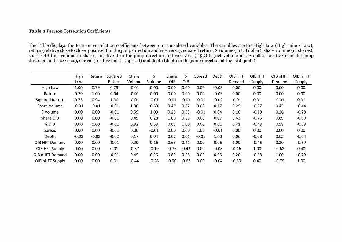
Table 2 Pearson Correlation Coefficients
The Table displays the Pearson correlation coefficients between our considered variables. The variables are the High Low (High minus Low), return (relative close to close, positive if in the jump direction and vice versa), squared return, $ volume (in US dollar), share volume (in shares), share OIB (net volume in shares, positive if in the jump direction and vice versa), $ OIB (net volume in US dollar, positive if in the jump direction and vice versa), spread (relative bid-ask spread) and depth (depth in the jump direction at the best quote).
High Low
Return Squared Return
Share Volume
$ Volume
Share OIB
$ OIB
Spread Depth OIB HFT Demand
OIB HFT Supply
OIB nHFT Demand
OIB nHFT Supply
High Low 1.00 0.79 0.73 -0.01 0.00 0.00 0.00 0.00 -0.03 0.00 0.00 0.00 0.00
Return 0.79 1.00 0.94 -0.01 0.00 0.00 0.00 0.00 -0.03 0.00 0.00 0.00 0.00
Squared Return 0.73 0.94 1.00 -0.01 -0.01 -0.01 -0.01 -0.01 -0.02 -0.01 0.01 -0.01 0.01
Share Volume -0.01 -0.01 -0.01 1.00 0.59 0.49 0.32 0.00 0.17 0.29 -0.37 0.45 -0.44
$ Volume 0.00 0.00 -0.01 0.59 1.00 0.28 0.53 -0.01 0.04 0.16 -0.19 0.26 -0.28
Share OIB 0.00 0.00 -0.01 0.49 0.28 1.00 0.65 0.00 0.07 0.63 -0.76 0.89 -0.90
$ OIB 0.00 0.00 -0.01 0.32 0.53 0.65 1.00 0.00 0.01 0.41 -0.43 0.58 -0.63
Spread 0.00 0.00 -0.01 0.00 -0.01 0.00 0.00 1.00 -0.01 0.00 0.00 0.00 0.00
Depth -0.03 -0.03 -0.02 0.17 0.04 0.07 0.01 -0.01 1.00 0.06 -0.08 0.05 -0.04
OIB HFT Demand 0.00 0.00 -0.01 0.29 0.16 0.63 0.41 0.00 0.06 1.00 -0.46 0.20 -0.59
OIB HFT Supply 0.00 0.00 0.01 -0.37 -0.19 -0.76 -0.43 0.00 -0.08 -0.46 1.00 -0.68 0.40
OIB nHFT Demand 0.00 0.00 -0.01 0.45 0.26 0.89 0.58 0.00 0.05 0.20 -0.68 1.00 -0.79
OIB nHFT Supply 0.00 0.00 0.01 -0.44 -0.28 -0.90 -0.63 0.00 -0.04 -0.59 0.40 -0.79 1.00

Table 3 HFT trading activity around jumps
The table reports the ratio of the average HFT (nHFT) trading volume (in shares) during and around jump intervals over the average HFT (nHFT) trading volume (in shares) during non-jump intervals. HFT (nHFT) All sums up aggressive and passive HFT (nHFT) volume, HFT (nHFT) Supply is passive HFT (nHFT) volume and HFT (nHFT) Demand is aggressive HFT (nHFT) volume.
t-2 t-1 T t+1 t+2
HFT All 90.5% *** 127.0% *** 118.0% *** 130.6% *** 110.2% ***
(5.13) (5.36) (6.18) (7.1) (6.74)
HFT Demand 66.8% *** 104.5% *** 85.3% *** 107.2% *** 89.8% ***
(4.38) (5.57) (5.47) (6.83) (6.43)
HFT Supply 107.0% *** 138.6% *** 134.5% *** 147.1% *** 126.8% ***
(5.13) (4.83) (5.81) (6.64) (6.44)
t-2 t-1 T t+1 t+2
nHFT All 113.6% *** 146.7% *** 158.5% *** 142.2% *** 115.0% ***
(5.22) (4.81) (7) (7.3) (6.9)
nHFT Demand 135.3% *** 163.2% *** 186.7% *** 159.7% *** 130.2% ***
(5.26) (4.38) (6.8) (7.01) (6.69)
nHFT Supply 110.3% *** 142.2% *** 159.7% *** 131.7% *** 102.5% ***
(4.62) (4.41) (6.63) (6.69) (6.45)
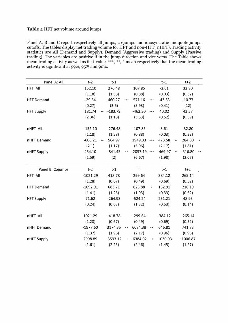
Table 4 HFT net volume around jumps
Panel A, B and C report respectively all jumps, co-jumps and idiosyncratic midquote jumps cutoffs. The tables display net trading volume for HFT and non-HFT (nHFT). Trading activity statistics are All (Demand and Supply), Demand (Aggressive trading) and Supply (Passive trading). The variables are positive if in the jump direction and vice versa. The Table shows mean trading activity as well as its t-value. ***, **, * mean respectively that the mean trading activity is significant at 99%, 95% and 90%.
Panel A: All t-2 t-1 T t+1 t+2
HFT All 152.10 276.48 107.85 -3.61 32.80
(1.18) (1.58) (0.88) (0.03) (0.32)
HFT Demand -29.64 460.27 *** 571.16 *** -43.63 -10.77
(0.27) (3.6) (5.93) (0.41) (12)
HFT Supply 181.74 ** -183.79 -463.30 *** 40.02 43.57
(2.36) (1.18) (5.53) (0.52) (0.59)
nHFT All -152.10 -276.48 -107.85 3.61 -32.80
(1.18) (1.58) (0.88) (0.03) (0.32)
nHFT Demand -606.21 ** 564.97 1949.33 *** 473.58 ** 284.00 *
(2.1) (1.17) (5.96) (2.17) (1.81)
nHFT Supply 454.10 -841.45 ** -2057.19 *** -469.97 ** -316.80 **
(1.59) (2) (6.67) (1.98) (2.07)
Panel B: Cojumps t-2 t-1 T t+1 t+2
HFT All -1021.29 418.78 299.64 384.12 265.14
(1.28) (0.67) (0.49) (0.69) (0.52)
HFT Demand -1092.91 683.71 823.88 * 132.91 216.19
(1.41) (1.25) (1.93) (0.33) (0.62)
HFT Supply 71.62 -264.93 -524.24 251.21 48.95
(0.24) (0.63) (1.32) (0.53) (0.14)
nHFT All 1021.29 -418.78 -299.64 -384.12 -265.14
(1.28) (0.67) (0.49) (0.69) (0.52)
nHFT Demand -1977.60 3174.35 ** 6084.38 ** 646.81 741.73
(1.37) (1.96) (2.17) (0.96) (0.96)
nHFT Supply 2998.89 -3593.12 ** -6384.02 ** -1030.93 -1006.87
(1.61) (2.25) (2.46) (1.45) (1.27)

Panel C: Idiosyncratic jumps t-2 t-1 T t+1 t+2
HFT All 281.48 ** 260.86 87.69 -46.09 7.21
(2.51) (1.43) (0.73) (0.42) (0.07)
HFT Demand 87.60 435.74 *** 544.58 *** -62.98 -35.76
(1.04) (3.39) (5.65) (0.58) (0.41)
HFT Supply 193.88 ** -174.88 -456.90 *** 16.89 42.98
(2.46) (1.05) (5.53) (0.25) (0.58)
nHFT All -281.48 -260.86 -87.69 46.09 -7.21
(2.51) (1.43) (0.73) (0.42) (0.07)
nHFT Demand -455.00 278.47 1514.56 *** 454.60 ** 233.58
(1.63) (0.55) (7.3) (1.97) (1.54)
nHFT Supply 173.52 -539.33 -1602.25 *** -408.51 -240.80 *
(0.72) (1.24) (7.89) (1.62) (1.65)

Table 5 HFT net volume around jumps
Panel A, B and C report respectively all jumps, co-jumps and idiosyncratic transaction jumps cutoffs. The tables display net trading volume for HFT and non-HFT (nHFT). Trading activity statistics are All (Demand and Supply), Demand (Aggressive trading) and Supply (Passive trading). The variables are positive if in the jump direction and vice versa. The Table shows mean trading activity as well as its t-value. ***, **, * mean respectively that the mean trading activity is significant at 99%, 95% and 90%.
Panel A: All t-2 t-1 t t+1 t+2
HFT All -140.61 -279.44 -2082.14 *** -633.94 * 97.90
(0.40) (0.77) (4.68) (1.68) (0.28)
HFT Demand -437.82 425.76 2146.95 *** -665.65 * 59.37
(1.2) (1.62) (5.18) (1.8) (0.18)
HFT Supply 297.21 -705.20 -4229.09 *** 31.71 38.53
(0.69) (1.62) (8.55) (0.07) (0.11)
nHFT All 140.61 279.44 2082.14 *** 633.94 * -97.90
(0.4) (0.77) (4.68) (1.68) (0.28)
nHFT Demand -328.23 2091.15 ** 14395.93 *** 2239.19 *** 1794.74 **
(0.38) (2.38) (13.79) (2.92) (2.38)
nHFT Supply 468.84 -1811.71 ** -12313.8 *** -1605.25 ** -1892.65 ***
(0.59) (2.44) (14.02) (2.29) (2.63)
Panel B: Cojumps t-2 t-1 t t+1 t+2
HFT All -518.33 * 499.02 -1477.63 *** -155.91 -0.55
(1.65) (1.41) (3.66) (0.56) (0.002)
HFT Demand -465.04 685.37 * 545.48 ** -62.62 58.00
(1.27) (1.94) (2.19) (0.3) (0.31)
HFT Supply -53.29 -186.35 -2023.11 *** -93.29 -58.55
(0.22) (0.84) (5.52) (0.57) (0.4)
nHFT All 518.33 * -499.02 1477.64 *** 155.91 0.55
(1.65) (1.41) (3.66) (0.56) (0.002)
nHFT Demand -626.28 1406.65 6877.27 *** 1242.96 2313.56 **
(0.64) (1.45) (6.79) (1.3) (2.19)
nHFT Supply 1144.62 -1905.67 * -5399.63 *** -1087.05 -2313.02 **
(1.08) (1.78) (6.24) (1.03) (2.08)

Panel C: Idiosyncratic jumps t-2 t-1 t t+1 t+2
HFT All 108.65 -793.14 -2481.05 *** -949.39 162.87
(0.2) (1.42) (3.6) (1.58) (0.29)
HFT Demand -419.86 254.44 3203.75 *** -1063.58 * 60.28
(0.75) (0.69) (4.8) (1.78) (0.11)
HFT Supply 528.50 -1047.59 -6584.80 *** 114.19 102.59
(0.76) (1.48) (7.26) (0.16) (0.17)
nHFT All -108.65 793.14 2481.05 *** 949.39 -162.87
(0.19) (1.43) (3.6) (1.58) (0.29)
nHFT Demand -131.55 2542.85 * 19357.44 *** 2896.60 *** 1452.37
(0.1) (1.94) (12.18) (2.62) (1.39)
nHFT Supply 22.89 -1749.71 * -16876 *** -1947.21 ** -1615.24 *
(0.02) (1.73) (12.67) (2.09) (1.71)

Table 6 HFT net volume around permanent and transitory jumps
Panel A and B report respectively permanent jumps and transitory midquote jumps cutoffs. The tables display net trading volume for HFT and non-HFT (nHFT). Trading activity statistics are All (Demand and Supply), Demand (Aggressive trading) and Supply (Passive trading). The variables are positive if in the jump direction and vice versa. The Table shows mean trading activity as well as its t-value. ***, **, * mean respectively that the mean trading activity is significant at 99%, 95% and 90%.
Panel A: Permanent Jumps t-2 t-1 T t+1 t+2
HFT All 356.80 * 417.38 206.68 49.49 53.71
(1.87) (1.46) (0.94) (0.27) (0.3)
HFT Demand 56.53 985.80 *** 820.71 *** -118.05 -55.57
(0.39) (4.33) (4.8) (0.68) (0.38)
HFT Supply 300.27 ** -568.42 ** -614.03 *** 167.54 109.28
(2.24) (2.25) (4.22) (1.23) (0.85)
nHFT All -356.80 -417.38 -206.68 -49.49 -53.71
(1.87) (1.46) (0.94) (0.27) (0.3)
nHFT Demand -965.93 * 1459.08 * 3163.70 *** 495.70 402.38
(1.95) (1.75) (5.22) (1.33) (1.51)
nHFT Supply 609.13 -1876.46 ** -3370.38 *** -545.19 -456.09 *
(1.37) (2.49) (5.87) (1.41) (1.77)
Panel B: Transitory Jumps t-2 t-1 T t+1 t+2
HFT All -87.63 112.35 -1.07 -65.79 8.35
(0.52) (0.62) (0.012) (0.56) (0.11)
HFT Demand -130.56 -151.89 ** 296.11 *** 43.52 41.65
(0.81) (1.96) (4.05) (0.41) (0.56)
HFT Supply 42.93 264.24 -297.18 *** -109.32 ** -33.30
(0.75) (1.62) (4.09) (2) (0.59)
nHFT All 87.63 -112.35 1.07 65.79 -8.35
(0.52) (0.62) (0.012) (0.56) (0.11)
nHFT Demand -184.91 -476.55 610.91 *** 447.68 ** 145.50
(0.77) (1.23) (3.87) (2.42) (1.05)
nHFT Supply 272.54 364.20 -609.85 *** -381.88 -153.85
(0.8) (1.47) (4.55) (1.53) (1.1)

Table 7 HFT net volume around permanent and transitory jumps
Panel A and B report respectively permanent jumps and transitory transaction jumps cutoffs. The tables display net trading volume for HFT and non-HFT (nHFT). Trading activity statistics are All (Demand and Supply), Demand (Aggressive trading) and Supply (Passive trading). The variables are positive if in the jump direction and vice versa. The Table shows mean trading activity as well as its t-value. ***, **, * mean respectively that the mean trading activity is significant at 99%, 95% and 90%.
Panel A: Permanent Jumps t-2 t-1 T t+1 t+2
HFT All -283.31 38.64 -2223.63 *** -258.60 21.27
(0.8) (0.096) (4.67) (0.67) (0.053)
HFT Demand -256.36 388.33 2328.40 *** 61.55 369.34
(0.61) (1.37) (6.01) (0.21) (0.96)
HFT Supply -26.95 -349.69 -4452.03 *** -320.15 -348.07
(0.065) (0.75) (7.76) (0.64) (0.84)
nHFT All 283.31 -38.64 2223.63 *** 258.60 -21.27
(0.8) (0.096) (4.67) (0.67) (0.053)
nHFT Demand -662.92 1342.21 15438.46 *** 3194.38 *** 3250.57 ***
(0.74) (1.29) (12.62) (3.85) (3.63)
nHFT Supply 946.23 -1380.85 -13214.83 *** -2935.78 *** -3271.84 ***
(1.09) (1.64) (13.30) (4.52) (3.77)
Panel B: Transitory Jumps t-2 t-1 T t+1 t+2
HFT All 359.21 -1393.55 -1586.56 -1948.62 * 366.31
(0.36) (1.64) (1.43) (1.88) (0.48)
HFT Demand -1073.40 556.87 1511.37 -3212.75 ** -1026.35
(1.43) (0.86) (1.18) (2.44) (1.46)
HFT Supply 1432.61 -1950.42 * -3097.93 *** 1264.13 1392.66 **
(1.14) (1.78) (3.61) (1.51) (2)
nHFT All -359.21 1393.55 1586.56 1948.62 * -366.31
(0.36) (1.64) (1.43) (1.88) (0.48)
nHFT Demand 844.08 4714.39 *** 10744.34 *** -1106.49 -3304.48 **
(0.37) (3.04) (5.58) (0.59) (2.55)
nHFT Supply -1203.28 -3320.84 ** -9157.77 *** 3055.11 2938.16 ***
(0.65) (2.1) (4.89) (1.4) (2.68)

Table 8 Drivers of price jumps occurrence
The table is a probit regression with fixed effects. The dependent variable takes 1 when a jump occurs and 0 otherwise. The independent variables are defined such as in Table 1. We report the results for the permanent / transitory cutoff. The Table shows the parameter estimates as well as their wald chi-square. ***, **, * mean respectively that the parameter is significant at 99%, 95% and 90%. The marginal effect (ME) of each explanatory variable is also reported.
Panel A: Permanent Jumps Scaling Coef. ME Coef. ME Coef. ME
High Low (t-1) 1.E+03 2623.80 *** 0.50 2622.90 *** 0.50 2622.60 *** 0.50
(192.69)
(192.56)
(192.52)
Return (t-1) 1.E+03 3254 *** 0.62 3287 *** 0.63 3220 *** 0.61
(12.81)
(12.95)
(12.24)
Squared Return (t-1) 1.E+03 -23699 *** -4.53 -23880 *** -4.57 -23483 *** -4.48
(21.42)
(21.50)
(20.56)
Share Volume (t-1) 1.E+08 247.00 *** 0.05 248.70 *** 0.05 256.40 *** 0.05
(535.45)
(517.82)
(548.39)
$ Volume ( t-1) 1.E+09 28.15 *** 0.01 27.95 *** 0.01 26.37 *** 0.01
(46.14)
(47.28)
(39.28)
$ Volume (t) 1.E+09 0.32
0.00 1.70
0.00 2.01
0.00
(0.01)
(0.17)
(0.22)
Spread (t-1) 1.E+01 210.00 *** 0.04 210.20 *** 0.04 210.00 *** 0.04
(182.32)
(183.15)
(182.21)
Depth (t-1) 1.E+06 -1228.80 *** -0.23 -1224.90 *** -0.23 -1230.10 *** -0.23
(154.73)
(153.69)
(155.23)
OIB HFT (t) 1.E+08 82.80
0.02
(1.44)
OIB HFT Demand (t) 1.E+08
-12.06
0.00
(0.02)
OIB HFT Supply (t) 1.E+08
112.40 * 0.02
(1.87)
OIB nHFT Demand (t) 1.E+08
-52.74 *** -0.01
(4.69)
OIB nHFT Supply (t) 1.E+08
35.02 ** 0.01
(2.17)
OIB HFT (t-1) 1.E+08 103.00 *** 0.02
(6.52)
OIB HFT Demand (t-1) 1.E+08
29.63
0.01
(0.47)
OIB HFT Supply (t-1) 1.E+08
142.60 *** 0.03
(8.29)
OIB nHFT Demand (t-1) 1.E+08
-11.45
0.00
(0.38)
OIB nHFT Supply (t-1) 1.E+08
-27.83 * -0.01
(1.87)
Pseudo R^2
4.89%
4.88%
4.91%

Panel B: Transitory Jumps Scaling Coef. ME Coef. ME Coef. ME
High Low (t-1) 1.E+03 2551.80 *** 0.03 2548.90 *** 0.03 2554.10 *** 0.03
(26.38)
(26.32)
(26.50)
Return (t-1) 1.E+03 -37711 *** -0.49 -37134 *** -0.48 -36132 *** -0.48
(42.04)
(45.10)
(46.56)
Squared Return (t-1) 1.E+03 -434769 *** -5.67 -426111 *** -5.52 -408942 *** -5.39
(18.50)
(20.16)
(21.04)
Share Volume (t-1) 1.E+08 106.80 *** 0.00 112.80 *** 0.00 118.60 *** 0.00
(34.79)
(32.25)
(35.97)
$ Volume ( t-1) 1.E+09 30.66 *** 0.00 28.36 *** 0.00 27.79 *** 0.00
(26.55)
(18.95)
(20.26)
$ Volume (t) 1.E+09 10.36 *** 0.00 11.56 *** 0.00 12.11 *** 0.00
(3.81)
(3.48)
(4.77)
Spread (t-1) 1.E+01 218.20 *** 0.00 217.90 *** 0.00 217.90 *** 0.00
(62.81)
(62.52)
(62.37)
Depth (t-1) 1.E+06 -775.10 *** -0.01 -818.50 *** -0.01 -821.80 *** -0.01
(10.26)
(10.95)
(10.88)
OIB HFT (t) 1.E+08 -232.70 *** 0.00
(5.34)
OIB HFT Demand (t) 1.E+08
-113.80
0.00
(0.76)
OIB HFT Supply (t) 1.E+08
-101.90
0.00
(0.52)
OIB nHFT Demand (t) 1.E+08
21.73
0.00
(0.24)
OIB nHFT Supply (t) 1.E+08
26.57
0.00
(0.82)
OIB HFT (t-1) 1.E+08 -15.44
0.00
(0.02)
OIB HFT Demand (t-1) 1.E+08
-257.90 *** 0.00
(6.87)
OIB HFT Supply (t-1) 1.E+08
275.90 *** 0.00
(6.81)
OIB nHFT Demand (t-1) 1.E+08
5.25
0.00
(0.02)
OIB nHFT Supply (t-1) 1.E+08
-17.23
0.00
(0.23)
Pseudo R^2
6.33%
6.39%
6.43%

Table 9 Drivers of price jumps size
The table is a panel regression with fixed effects on jump intervals. The dependent variable is the High Low during the 10-second jump interval. The independent variables are defined such as in Table 1. We report the results for the permanent / transitory cutoff. The Table shows the parameter estimates as well as their t-stat. ***, **, * mean respectively that the parameter is significant at 99%, 95% and 90%.
Panel A: Permanent Jumps Scaling Coef. Coef. Coef.
High Low (t-1) 1.E+03 249.43 *** 253.80 *** 253.84 ***
(8.35)
(8.49)
(8.47) Return (t-1) 1.E+03 9.20
17.61
18.59
(0.59)
(1.05)
(1.12) Squared Return (t-1) 1.E+03 277.34 *** 250.16 *** 245.40 ***
(4.08)
(3.54)
(3.49) Share Volume (t-1) 1.E+08 0.40
0.29
0.25
(1.51)
(1.07)
(0.91) $ Volume ( t-1) 1.E+09 -0.45 *** -0.44 *** -0.42 **
(2.73)
(2.57)
(2.47) $ Volume (t) 1.E+09 0.47 *** 0.46 *** 0.46 ***
(3.29)
(3.10)
(3.10) Spread (t-1) 1.E+01 -0.27
-0.27
-0.27
(0.32)
(0.32)
(0.32) Depth (t-1) 1.E+06 -2.73 *** -2.91 *** -2.71 ***
(2.81)
(2.97)
(2.83) OIB HFT (t) 1.E+08 0.58
(0.64)
OIB HFT Demand (t) 1.E+08
1.94 *
(1.70) OIB HFT Supply (t) 1.E+08
-0.67
(0.56) OIB nHFT Demand (t) 1.E+08
0.40
(0.67) OIB nHFT Supply (t) 1.E+08
-0.41
(0.53) OIB HFT (t-1) 1.E+08 0.79
(1.49)
OIB HFT Demand (t-1) 1.E+08
0.10
(0.15) OIB HFT Supply (t-1) 1.E+08
0.37
(0.60) OIB nHFT Demand (t-1) 1.E+08
-0.55 ***
(3.17) OIB nHFT Supply (t-1) 1.E+08
0.54 **
(2.08) Adjusted R^2
76.03%
76.17%
76.12%

Panel B: Transitory Jumps Scaling Coef. Coef. Coef.
High Low (t-1) 1.E+03 248.64
261.09
255.90
(1.22)
(1.18)
(1.16) Return (t-1) 1.E+03 -404.83 *** -414.54 ** -413.21 **
(2.73)
(2.41)
(2.50) Squared Return (t-1) 1.E+03 7142.05
5900.05
6542.70
(0.71)
(0.51)
(0.60) Share Volume (t-1) 1.E+08 0.13
-0.22
-0.33
(0.11)
(0.13)
(0.19) $ Volume ( t-1) 1.E+09 -0.34
-0.25
-0.21
(0.73)
(0.44)
(0.46) $ Volume (t) 1.E+09 1.02 ** 0.96 ** 0.88 *
(2.16)
(2.08)
(1.90) Spread (t-1) 1.E+01 -1.20
-1.21
-1.22
(1.19)
(1.21)
(1.21) Depth (t-1) 1.E+06 -2.75
-1.44
-2.73
(0.87)
(0.41)
(0.80) OIB HFT (t) 1.E+08 -0.45
(0.13)
OIB HFT Demand (t) 1.E+08
0.26
(0.11) OIB HFT Supply (t) 1.E+08
-20.68
(0.99) OIB nHFT Demand (t) 1.E+08
2.88
(0.77) OIB nHFT Supply (t) 1.E+08
-0.24
(0.08) OIB HFT (t-1) 1.E+08 -0.13
(0.06)
OIB HFT Demand (t-1) 1.E+08
-1.37
(0.28) OIB HFT Supply (t-1) 1.E+08
-8.60
(1.12) OIB nHFT Demand (t-1) 1.E+08
-0.03
(0.02) OIB nHFT Supply (t-1) 1.E+08
1.86
(0.76) Adjusted R^2
81.84%
81.94%
82.47%
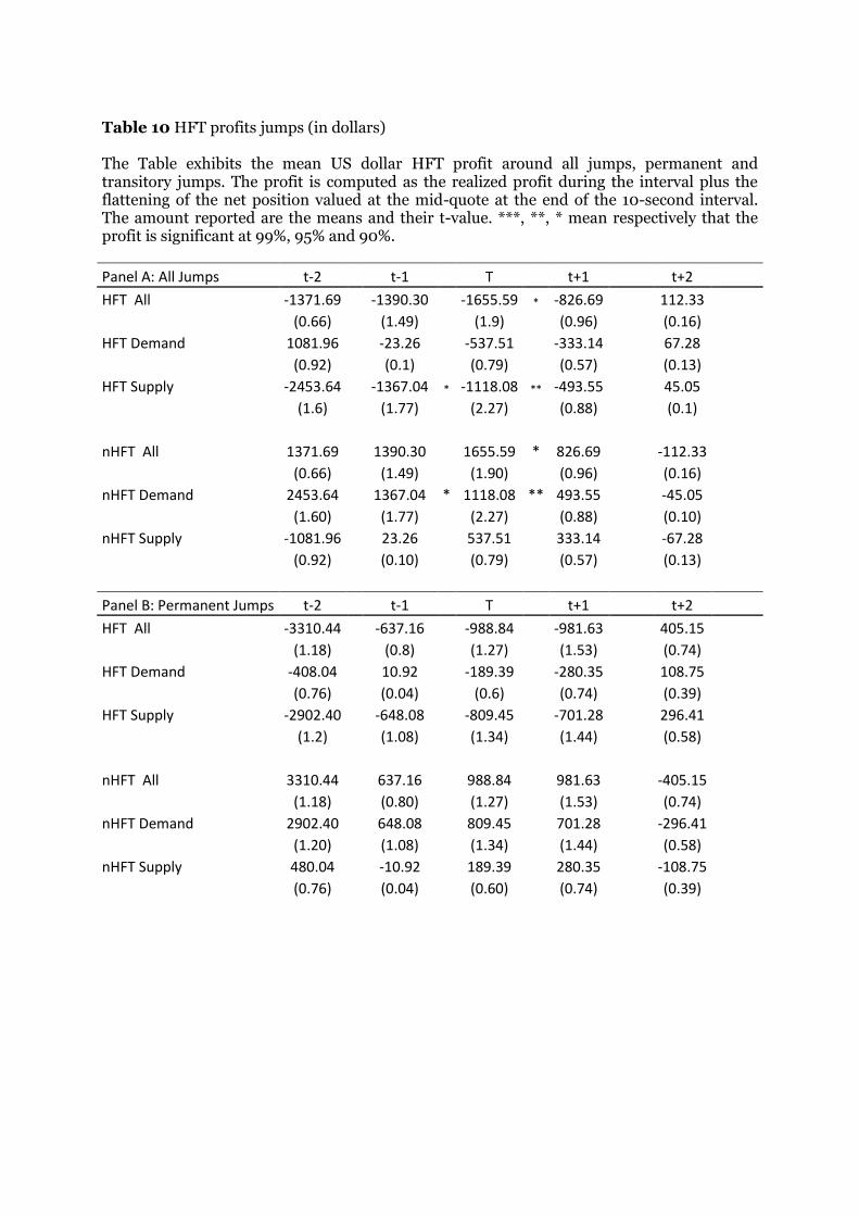
Table 10 HFT profits jumps (in dollars)
The Table exhibits the mean US dollar HFT profit around all jumps, permanent and transitory jumps. The profit is computed as the realized profit during the interval plus the flattening of the net position valued at the mid-quote at the end of the 10-second interval. The amount reported are the means and their t-value. ***, **, * mean respectively that the profit is significant at 99%, 95% and 90%.
Panel A: All Jumps t-2 t-1 T t+1 t+2
HFT All -1371.69 -1390.30 -1655.59 * -826.69 112.33
(0.66) (1.49) (1.9) (0.96) (0.16)
HFT Demand 1081.96 -23.26 -537.51 -333.14 67.28
(0.92) (0.1) (0.79) (0.57) (0.13)
HFT Supply -2453.64 -1367.04 * -1118.08 ** -493.55 45.05
(1.6) (1.77) (2.27) (0.88) (0.1)
nHFT All 1371.69 1390.30 1655.59 * 826.69 -112.33
(0.66) (1.49) (1.90) (0.96) (0.16)
nHFT Demand 2453.64 1367.04 * 1118.08 ** 493.55 -45.05
(1.60) (1.77) (2.27) (0.88) (0.10)
nHFT Supply -1081.96 23.26 537.51 333.14 -67.28
(0.92) (0.10) (0.79) (0.57) (0.13)
Panel B: Permanent Jumps t-2 t-1 T t+1 t+2
HFT All -3310.44 -637.16 -988.84 -981.63 405.15
(1.18) (0.8) (1.27) (1.53) (0.74)
HFT Demand -408.04 10.92 -189.39 -280.35 108.75
(0.76) (0.04) (0.6) (0.74) (0.39)
HFT Supply -2902.40 -648.08 -809.45 -701.28 296.41
(1.2) (1.08) (1.34) (1.44) (0.58)
nHFT All 3310.44 637.16 988.84 981.63 -405.15
(1.18) (0.80) (1.27) (1.53) (0.74)
nHFT Demand 2902.40 648.08 809.45 701.28 -296.41
(1.20) (1.08) (1.34) (1.44) (0.58)
nHFT Supply 480.04 -10.92 189.39 280.35 -108.75
(0.76) (0.04) (0.60) (0.74) (0.39)

Panel C: Transitory Jumps t-2 t-1 T t+1 t+2
HFT All 1708.18 -10787.94 -2477.69 -576.28 -376.99
(0.56) (1.4) (1.46) (0.29) (0.23)
HFT Demand 3448.93 -449.73 -973.27 -418.46 -2.01
(1.17) (0.84) (0.65) (0.3) (0.001)
HFT Supply -1740.75 * -10338.20 -1504.42 * -157.82 -374.98
(1.79) (1.43) (1.86) (0.13) (0.42)
nHFT All -1708.18 10787.94 2477.69 576.28 376.99
(0.56) (1.40) (1.46) (0.29) (0.23)
nHFT Demand 1740.75 10338.20 1504.42 * 157.82 374.98
(1.79) (1.43) (1.86) (0.13) (0.42)
nHFT Supply -3448.93 449.73 973.27 418.46 2.01
(1.17) (0.84) (0.65) (0.30) (0.00)
Recommended